Lecture 11 - The Karush-Kuhn-Tucker Conditions · Lecture 11 - The Karush-Kuhn-Tucker Conditions ... De nition.Consider the problem min h(x) ... Amir Beck\Introduction to Nonlinear

$Page 1: Lecture 11 - The Karush-Kuhn-Tucker Conditions · Lecture 11 - The Karush-Kuhn-Tucker Conditions ... De nition.Consider the problem min h(x) ... Amir Beck\Introduction to Nonlinear$
Lecture 11 - The Karush-Kuhn-Tucker Conditions

I The Karush-Kuhn-Tucker conditions are optimality conditions for inequalityconstrained problems discovered in 1951 (originating from Karush’s thesisfrom 1939).

I Modern nonlinear optimization essentially begins with the discovery of theseconditions.

The basic notion that we will require is the one of feasible descent directions.

Definition. Consider the problem

min h(x)s.t. x ∈ C ,

where h is continuously differentiable over the set C ⊆ Rn. Then a vectord 6= 0 is called a feasible descent direction at x ∈ C if ∇f (x)Td < 0 andthere exists ε > 0 such that x + td ∈ C for all t ∈ [0, ε].

Amir Beck “Introduction to Nonlinear Optimization” Lecture Slides - The KKT Conditions 1 / 34

The Basic Necessary Condition - No Feasible DescentDirections

Lemma. Consider the problem

(G)min h(x)s.t. x ∈ C ,

where h is continuously differentiable over C . If x∗ is a local optimalsolution of (G), then there are no feasible descent directions at x∗.

Proof.

I By contradiction, assume that there exists a vector d and ε1 > 0 such thatx + td ∈ C for all t ∈ [0, ε1] and ∇f (x∗)Td < 0.

I By definition of the directional derivative there exists ε2 < ε1 such thatf (x∗ + td) < f (x∗) for all t ∈ [0, ε2]⇒ contradiction to the local optimalityof x∗.


Consequence

Lemma. Let x∗ be a local minimum of the problem

min f (x)s.t. gi (x) ≤ 0, i = 1, 2, . . . ,m,

where f , g1, . . . , gm are continuously differentiable functions over Rn. LetI (x∗) be the set of active constraints at x∗:

I (x∗) = {i : gi (x∗) = 0}.

Then there there does not exist a vector d ∈ Rn such that

∇f (x∗)Td < 0,∇gi (x∗)Td < 0, i ∈ I (x∗)


Proof

I Suppose that d satisfies the system of inequalities.

I Then ∃ε1 > 0 such that f (x∗ + td) < f (x∗) and gi (x∗ + td) < gi (x∗) = 0 forany t ∈ (0, ε1) and i ∈ I (x∗).

I For any i /∈ I (x∗) we have that gi (x∗) < 0, and hence, by the continuity ofgi , there exists ε2 > 0 such that gi (x∗ + td) < 0 for any t ∈ (0, ε2) andi /∈ I (x∗).

I Consequently,f (x∗ + td) < f (x∗),gi (x∗ + td) < 0, i = 1, 2, . . . ,m,

for all t ∈ (0,min{ε1, ε2}).

I A contradiction to the local optimality of x∗.


The Fritz-John Necessary Condition

Theorem. Let x∗ be a local minimum of the problem

min f (x)s.t. gi (x) ≤ 0, i = 1, 2, . . . ,m,

where f , g1, . . . , gm are continuously differentiable functions over Rn. Thenthere exist multipliers λ0, λ1, . . . , λm ≥ 0, which are not all zeros, such that

λ0∇f (x∗) +m∑i=1

λi∇gi (x∗) = 0,

λigi (x∗) = 0, i = 1, 2, . . . ,m.


Proof of Fritz-John ConditionsI The following system is infeasible

(S) ∇f (x∗)Td < 0,∇gi (x∗)Td < 0, i ∈ I (x∗)

I System (S) is the same as Ad < 0 where A =

∇f (x∗)T

∇gi1(x∗)T

...∇gik (x∗)T

I By Gordan’s theorem of alternative, system (S) is infeasible if and only if

there exists a vector η = (λ0, λi1 , . . . , λik )T 6= 0 such that

ATη = 0,η ≥ 0,

I which is the same as λ0∇f (x∗) +∑

i∈I (x∗) λi∇gi (x∗) = 0.I Define λi = 0 for any i /∈ I (x∗), and we obtain that

λ0∇f (x∗) +m∑i=1

λi∇gi (x∗) = 0, λigi (x∗) = 0, i = 1, 2, . . . ,m


The KKT Conditions for Inequality Constrained Problems

A major drawback of the Fritz-John conditions is that they allow λ0 to be zero.Under an additional regularity condition, we can assume that λ0 = 1.

Theorem. Let x∗ be a local minimum of the problem

min f (x)s.t. gi (x) ≤ 0, i = 1, 2, . . . ,m,

where f , g1, . . . , gm are continuously differentiable functions over Rn. Sup-pose that the gradients of the active constraints {∇gi (x∗)}i∈I (x∗) are linearlyindependent. Then there exist multipliers λ1, λ2 . . . , λm ≥ 0 such that

∇f (x∗) +m∑i=1

λi∇gi (x∗) = 0,

λigi (x∗) = 0, i = 1, 2, . . . ,m.


Proof of the KKT Conditions for Inequality ConstrainedProblems

I By the Fritz-John conditions it follows that there exists λ0, λ1, . . . , λm, notall zeros, such that

λ0∇f (x∗) +m∑i=1

λi∇gi (x∗) = 0,

λigi (x∗) = 0, i = 1, 2, . . . ,m.

I λ0 6= 0 since otherwise, if λ0 = 0∑i∈I (x∗)

λi∇gi (x∗) = 0,

where not all the scalars λi , i ∈ I (x∗) are zeros, which is a contradiction tothe regularity condition.

I λ0 > 0. Defining λi = λi

λ0, the result follows.


KKT Conditions for Inequality/Equality ConstrainedProblems

Let x∗ be a local minimum of the problem

min f (x)s.t. gi (x) ≤ 0, i = 1, 2, . . . ,m,

hj(x) = 0, j = 1, 2, . . . , p.(1)

where f , g1, . . . , gm, h1, h2, . . . , hp are continuously differentiable functionsover Rn. Suppose that the gradients of the active constraints and the equal-ity constraints: {∇gi (x∗),∇hj(x∗), i ∈ I (x∗), j = 1, 2, . . . , p} are linearly in-dependent. Then there exist multipliers λ1, λ2 . . . , λm ≥ 0, µ1, µ2, . . . , µp ∈R such that

∇f (x∗) +m∑i=1

λi∇gi (x∗) +

p∑j=1

µj∇hj(x∗) = 0,

λigi (x∗) = 0, i = 1, 2, . . . ,m.


TerminologyDefinition (KKT point) Consider problem (1) wheref , g1, . . . , gm, h1, h2, . . . , hp are continuously differentiable functionsover Rn. A feasible point x∗ is called a KKT point if there existλ1, λ2 . . . , λm ≥ 0, µ1, µ2, . . . , µp ∈ R such that

∇f (x∗) +m∑i=1

λi∇gi (x∗) +

p∑j=1

µj∇hj(x∗) = 0,

λigi (x∗) = 0, i = 1, 2, . . . ,m.

Definition (regularity) A feasible point x∗ is called regular if the set{∇gi (x∗),∇hj(x∗), i ∈ I (x∗), j = 1, 2, . . . , p} is linearly independent.

I The KKT theorem states that a necessary local optimality condition of aregular point is that it is a KKT point.

I The additional requirement of regularity is not required in linearly constrainedproblems in which no such assumption is needed.


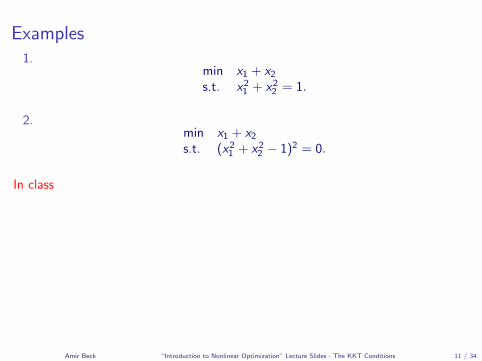
Examples1.

min x1 + x2s.t. x21 + x22 = 1.

2.min x1 + x2s.t. (x21 + x22 − 1)2 = 0.

In class


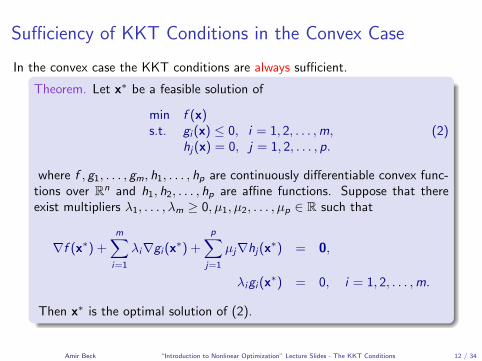
Sufficiency of KKT Conditions in the Convex Case

In the convex case the KKT conditions are always sufficient.

Theorem. Let x∗ be a feasible solution of

min f (x)s.t. gi (x) ≤ 0, i = 1, 2, . . . ,m,

hj(x) = 0, j = 1, 2, . . . , p.(2)

where f , g1, . . . , gm, h1, . . . , hp are continuously differentiable convex func-tions over Rn and h1, h2, . . . , hp are affine functions. Suppose that thereexist multipliers λ1, . . . , λm ≥ 0, µ1, µ2, . . . , µp ∈ R such that

∇f (x∗) +m∑i=1

λi∇gi (x∗) +

p∑j=1

µj∇hj(x∗) = 0,

λigi (x∗) = 0, i = 1, 2, . . . ,m.

Then x∗ is the optimal solution of (2).


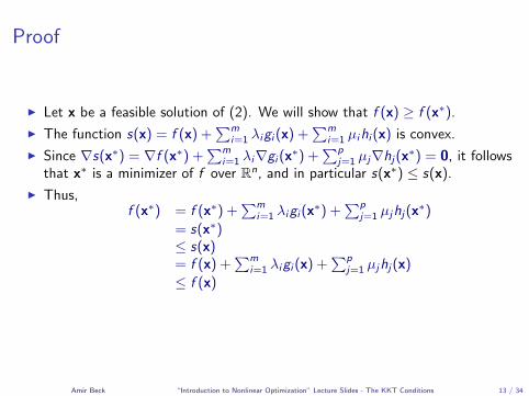
Proof

I Let x be a feasible solution of (2). We will show that f (x) ≥ f (x∗).

I The function s(x) = f (x) +∑m

i=1 λigi (x) +∑m

i=1 µihi (x) is convex.

I Since ∇s(x∗) = ∇f (x∗) +∑m

i=1 λi∇gi (x∗) +∑p

j=1 µj∇hj(x∗) = 0, it followsthat x∗ is a minimizer of f over Rn, and in particular s(x∗) ≤ s(x).

I Thus,f (x∗) = f (x∗) +

∑mi=1 λigi (x∗) +

∑pj=1 µjhj(x∗)

= s(x∗)≤ s(x)= f (x) +

∑mi=1 λigi (x) +

∑pj=1 µjhj(x)

≤ f (x)


The Convex Case - Necessity under Slater’s ConditionIn the convex case, the regularity condition can be replaced by Slater’s condition.

Theorem (necessity of the KKT conditions under Slater’s condition) Let x∗

be an optimal solution of the problem

min f (x)s.t. gi (x) ≤ 0, i = 1, 2, . . . ,m.

(3)

where f , g1, . . . , gm are continuously differentiable convex functions overRn. Suppose that there exists x ∈ Rn such that

gi (x) < 0, i = 1, 2, . . . ,m.

Then there exist multipliers λ1, λ2 . . . , λm ≥ 0 such that

∇f (x∗) +m∑i=1

λi∇gi (x∗) = 0, (4)

λigi (x∗) = 0, i = 1, 2, . . . ,m. (5)


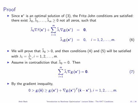
ProofI Since x∗ is an optimal solution of (3), the Fritz-John conditions are satisfied:

there exist λ0, λ1, . . . , λm ≥ 0 not all zeros, such that

λ0∇f (x∗) +m∑i=1

λi∇gi (x∗) = 0,

λigi (x∗) = 0, i = 1, 2, . . . ,m. (6)

I We will prove that λ0 > 0, and then conditions (4) and (5) will be satisfied

with λi = λi

λ0, i = 1, 2, . . . ,m.

I Assume in contradiction that λ0 = 0. Thenm∑i=1

λi∇gi (x∗) = 0. (7)

I By the gradient inequality,

0 > gi (x) ≥ gi (x∗) +∇gi (x∗)T (x− x∗), i = 1, 2, . . . ,m.


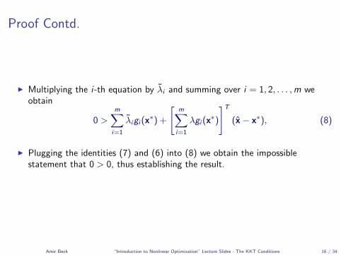
Proof Contd.

I Multiplying the i-th equation by λi and summing over i = 1, 2, . . . ,m weobtain

0 >m∑i=1

λigi (x∗) +

[m∑i=1

λgi (x∗)

]T(x− x∗), (8)

I Plugging the identities (7) and (6) into (8) we obtain the impossiblestatement that 0 > 0, thus establishing the result.


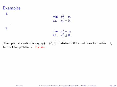
Examples1.

min x21 − x2s.t. x2 = 0.

.

2.min x21 − x2s.t. x22 ≤ 0.

The optimal solution is (x1, x2) = (0, 0). Satisfies KKT conditions for problem 1,but not for problem 2. In class


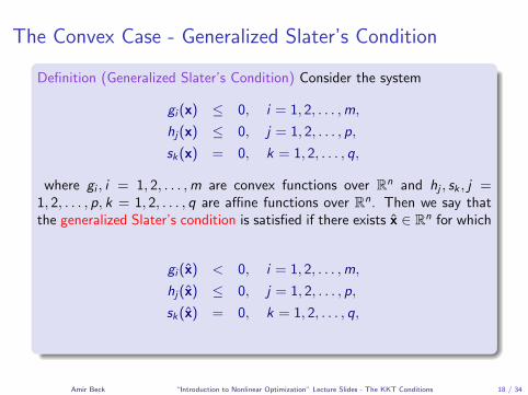
The Convex Case - Generalized Slater’s Condition

Definition (Generalized Slater’s Condition) Consider the system

gi (x) ≤ 0, i = 1, 2, . . . ,m,

hj(x) ≤ 0, j = 1, 2, . . . , p,

sk(x) = 0, k = 1, 2, . . . , q,

where gi , i = 1, 2, . . . ,m are convex functions over Rn and hj , sk , j =1, 2, . . . , p, k = 1, 2, . . . , q are affine functions over Rn. Then we say thatthe generalized Slater’s condition is satisfied if there exists x ∈ Rn for which

gi (x) < 0, i = 1, 2, . . . ,m,

hj(x) ≤ 0, j = 1, 2, . . . , p,

sk(x) = 0, k = 1, 2, . . . , q,


Necessity of KKT under Generalized SlaterTheorem. Let x∗ be an optimal solution of the problem

min f (x)s.t. gi (x) ≤ 0, i = 1, 2, . . . ,m,

hj(x) ≤ 0, j = 1, 2, . . . , p,sk(x) = 0, k = 1, 2, . . . , q,

(9)

where f , g1, . . . , gm are continuously differentiable convex functions andhj , sk , j = 1, 2, . . . , p, k = 1, 2, . . . , q are affine. Suppose that thegeneralized Slater’s condition is satisfied. Then there exist multipliersλ1, λ2 . . . , λm, η1, η2, . . . , ηp ≥ 0, µ1, µ2, . . . , µq ∈ R such that

∇f (x∗) +m∑i=1

λi∇gi (x∗) +

p∑j=1

ηj∇hj(x∗) +

q∑k=1

µk∇sk(x∗) = 0,

λigi (x∗) = 0, i = 1, 2, . . . ,m,

ηjhj(x∗) = 0, j = 1, 2, . . . , p.


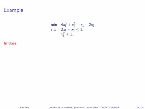
Example

min 4x21 + x22 − x1 − 2x2s.t. 2x1 + x2 ≤ 1,

x21 ≤ 1.

In class


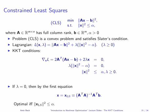
Constrained Least Squares

(CLS)min ‖Ax− b‖2,s.t. ‖x‖2 ≤ α,

where A ∈ Rm×n has full column rank, b ∈ Rm, α > 0

I Problem (CLS) is a convex problem and satisfies Slater’s condition.

I Lagrangian: L(x, λ) = ‖Ax− b‖2 + λ(‖x‖2 − α). (λ ≥ 0)

I KKT conditions:

∇xL = 2AT (Ax− b) + 2λx = 0,

λ(‖x‖2 − α) = 0,

‖x‖2 ≤ α, λ ≥ 0.

I If λ = 0, then by the first equation

x = xLS ≡ (ATA)−1ATb.

Optimal iff ‖xLS‖2 ≤ α.Amir Beck “Introduction to Nonlinear Optimization” Lecture Slides - The KKT Conditions 21 / 34

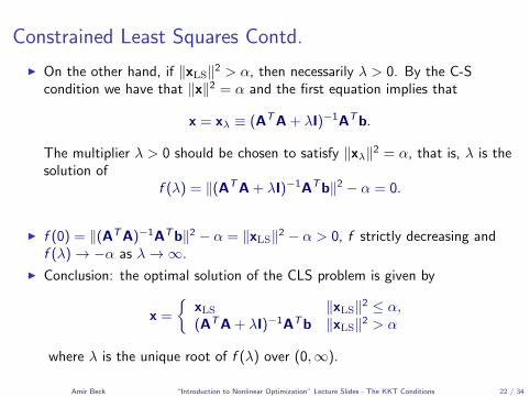
Constrained Least Squares Contd.

I On the other hand, if ‖xLS‖2 > α, then necessarily λ > 0. By the C-Scondition we have that ‖x‖2 = α and the first equation implies that

x = xλ ≡ (ATA + λI)−1ATb.

The multiplier λ > 0 should be chosen to satisfy ‖xλ‖2 = α, that is, λ is thesolution of

f (λ) = ‖(ATA + λI)−1ATb‖2 − α = 0.

I f (0) = ‖(ATA)−1ATb‖2 − α = ‖xLS‖2 − α > 0, f strictly decreasing andf (λ)→ −α as λ→∞.

I Conclusion: the optimal solution of the CLS problem is given by

x =

{xLS ‖xLS‖2 ≤ α,(ATA + λI)−1ATb ‖xLS‖2 > α

where λ is the unique root of f (λ) over (0,∞).


Second Order Necessary Optimality Conditions

Theorem. Consider the problem

min f (x)s.t. fi (x) ≤ 0, i = 1, 2, . . . ,m,

where f0, f1, . . . , fm are continuously differentiable over Rn. Let x∗ be a localminimum, and suppose that x∗ is regular meaning that {∇fi (x∗)}i∈I (x∗) arelinearly independent. Then ∃λ1, λ2, . . . , λm ≥ 0 such that

∇xL(x∗,λ) = 0,

λi fi (x∗) = 0, i = 1, 2, . . . ,m,

and yT∇2xxL(x∗,λ)y ≥ 0 for all y ∈ Λ(x∗) where

Λ(x∗) ≡ {d ∈ Rn : ∇fi (x∗)Td = 0, i ∈ I (x∗)}.

See proof of Theorem 11.18 in the book


Second Order Necessary Optimality Conditions forInequality/Equality Constrained Problems

Theorem. Consider the problem

min f (x)s.t. gi (x) ≤ 0, i = 1, 2, . . . ,m,

hj(x) = 0, j = 1, 2, . . . , p.

where f , g1, . . . , gm, h1, . . . , hp are continuously differentiable. Let x∗ bea local minimum and suppose that x∗ is regular meaning that the set{∇gi (x∗),∇hj(x∗), i ∈ I (x∗), j = 1, 2, . . . , p} is linearly independent. Then∃λ1, λ2, . . . , λm ≥ 0 and µ1, µ2, . . . , µp ∈ R such that

∇xL(x∗,λ,µ) = 0,

λigi (x∗) = 0, i = 1, 2, . . . ,m,

and dT∇2xxL(x∗,λ,µ)d ≥ 0 for all d ∈ Λ(x∗) ≡ {d ∈ Rn : ∇gi (x∗)Td =

0,∇hj(x∗)Td = 0, i ∈ I (x∗), j = 1, 2, . . . , p}.


Optimality Conditions for the Trust Region Subproblem

The Trust Region Subproblem (TRS) is the problem consisting of minimizing anindefinite quadratic function subject to an l2-norm constraint:

(TRS): min{f (x) ≡ xTAx + 2bTx + c : ‖x‖2 ≤ α},

where A = AT ∈ Rn×n,b ∈ Rn and c ∈ R. Although the problem is nonconvex,it possesses necessary and sufficient optimality conditions.

Theorem A vector x∗ is an optimal solution of problem (TRS) if and only ifthere exists λ∗ ≥ 0 such that

(A + λ∗I)x∗ = −b (10)

‖x∗‖2 ≤ α, (11)

λ∗(‖x∗‖2 − α) = 0, (12)

A + λ∗I � 0. (13)


ProofSufficiency:

I Assume that x∗ satisfies (10)-(13) for some λ∗ ≥ 0.

I Define the function

h(x) = xTAx+2bTx+c+λ∗(‖x‖2−α) = xT (A+λ∗I)x+2bTx+c−αλ∗. (14)

I Then by (13) we have that h is a convex quadratic function. By (10) itfollows that ∇h(x∗) = 0, which implies that x∗ is the unconstrainedminimizer of h over Rn.

I Let x be a feasible point, i.e., ‖x‖2 ≤ α. Then

f (x) ≥ f (x) + λ∗(‖x‖2 − α) (λ∗ ≥ 0, ‖x‖2 − α ≤ 0)= h(x) (by (14))≥ h(x∗) (x∗ is the minimizer of h)= f (x∗) + λ∗(‖x∗‖2 − α)= f (x∗) (by (12))


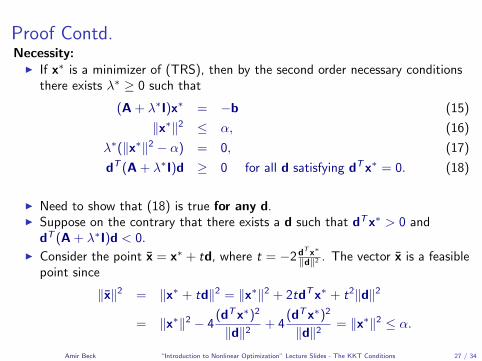
Proof Contd.Necessity:

I If x∗ is a minimizer of (TRS), then by the second order necessary conditionsthere exists λ∗ ≥ 0 such that

(A + λ∗I)x∗ = −b (15)

‖x∗‖2 ≤ α, (16)

λ∗(‖x∗‖2 − α) = 0, (17)

dT (A + λ∗I)d ≥ 0 for all d satisfying dTx∗ = 0. (18)

I Need to show that (18) is true for any d.I Suppose on the contrary that there exists a d such that dTx∗ > 0 and

dT (A + λ∗I)d < 0.

I Consider the point x = x∗ + td, where t = −2 dT x∗

‖d‖2 . The vector x is a feasiblepoint since

‖x‖2 = ‖x∗ + td‖2 = ‖x∗‖2 + 2tdTx∗ + t2‖d‖2

= ‖x∗‖2 − 4(dTx∗)2

‖d‖2+ 4

(dTx∗)2

‖d‖2= ‖x∗‖2 ≤ α.


Proof Contd.

I In addition,

f (x) = xTAx + 2bT x + c

= (x∗ + td)TA(x∗ + td) + 2bT (x∗ + td) + c

= (x∗)TAx∗ + 2bTx∗ + c︸︷︷︸f (x∗)

+t2dTAd + 2tdT (Ax∗ + b)

= f (x∗) + t2dT (A + λ∗I)d + 2tdT ((A + λ∗I)x∗ + b︸︷︷︸=0 by(15)

)

−λ∗t[t‖d‖2 + 2dTx∗

]︸︷︷︸=0

= f (x∗) + t2dT (A + λ∗I)d

< f (x∗),

which is a contradiction to the optimality of x∗.


Total Least SquaresConsider the approximate set of linear equations:

Ax ≈ b

I In the Least Squares (LS) approach we only assume that the RHS vector b issubjected to noise.

minw,x ‖w‖2s.t. Ax = b + w,

w ∈ Rm.

I In the Total Least Squares (TLS) we assume that both the RHS vector b andthe model matrix A are subjected to noise

(TLS)minE,w,x ‖E‖2F + ‖w‖2s.t. (A + E)x = b + w,

E ∈ Rm×n,w ∈ Rm.

The TLS problem – as formulated – seems like a difficult nonconvex problem. Wewill see that it can be solved efficiently.


Eliminating the E and w variablesI Fixing x, we will solve the problem

(Px)minE,w ‖E‖2F + ‖w‖2s.t. (A + E)x = b + w.

I The KKT conditions are necessary and sufficient for problem (Px).

I Lagrangian: L(E,w,λ) = ‖E‖2F + ‖w‖2 + 2λT [(A + E)x− b−w].

I By the KKT conditions, (E,w) is an optimal solution of (Px) if and only ifthere exists λ ∈ Rm such that

2E + 2λxT = 0 (∇EL = 0), (19)

2w − 2λ = 0 (∇wL = 0), (20)

(A + E)x = b + w (feasibility). (21)

I By (19), (20) and (21), E = −λxT ,w = λ and λ = Ax−b‖x‖2+1 . Plugging this

into the objectve function, a reduced formulation in the variables x isobtained.


The New Formulation of (TLS)

(TLS’) minx∈Rn

‖Ax− b‖2

‖x‖2 + 1.

Theorem x is an optimal solution of (TLS’) if and only if (x,E,w) is an

optimal solution of (TLS) where E = − (Ax−b)xT

‖x‖2+1 and w = Ax−b‖x‖2+1

I Still a nonconvex problem.I Resembles the problem of minimizing the Rayleigh quotient.


Solving the Fractional Quadratic Formulation

Under a rather mild condition, the optimal solution of (TLS’) can be derived via ahomogenization argument.

I (TLS’) is the same as

minx∈Rn,t∈R

{‖Ax− tb‖2

‖x‖2 + t2: t = 1

}.

I the same as (denoting y =

(xt

)):

f ∗ = miny∈Rn+1

{yTBy

‖y‖2: yn+1 = 1

}, (22)

where

B =

(ATA −ATb−bTA ‖b‖2

).


Solving the Fractional Quadratic Formulation Contd.We will consider the following relaxed version:

g∗ = miny∈Rn+1

{yTBy

‖y‖2: y 6= 0

}, (23)

Lemma. Let y∗ be an optimal solution of (23) and assume that y∗n+1 6= 0.Then y = 1

y∗n+1

y∗ is an optimal solution of (22).

Proof.

I f ∗ ≥ g∗.

I y is feasible for (22) and we have

f ∗ ≤ yTBy

‖y‖2=

1(y∗

n+1)2 (y∗)TBy∗

1(y∗

n+1)2 ‖y∗‖2

=(y∗)TBy∗

‖y∗‖2= g∗.

I Therefore, y is an optimal solution of both (22) and (23).


Main Result on TLSTheorem. Assume that the following condition holds:

λmin(B) < λmin(ATA), (24)

where

B =

(ATA −ATb−bTA ‖b‖2

).

Then the optimal solution of problem (TLS’) is given by 1yn+1

v, where

y =

(v

yn+1

)is an eigenvector corresponding to the min. eigenvalue of B.

Proof.I All we need to prove is that under condition (24), an optimal solution y∗ of

(23) must satisfy y∗n+1 6= 0.I Assume on the contrary that y∗n+1 = 0. Then

λmin(B) =(y∗)TBy∗

‖y∗‖2=

vTATAv

‖v‖2≥ λmin(ATA),

which is a contradiction to (24).Amir Beck “Introduction to Nonlinear Optimization” Lecture Slides - The KKT Conditions 34 / 34

Documents

Lecture 11 - The Karush-Kuhn-Tucker Conditions · Lecture 11 - The Karush-Kuhn-Tucker Conditions ... De nition.Consider the problem min h(x) ... Amir Beck\Introduction to Nonlinear