Embed Size (px)
Citation preview
Lecture 12Robust Estimation
Prof. Dr. Svetlozar RachevInstitute for Statistics and Mathematical Economics
University of Karlsruhe
Financial Econometrics, Summer Semester 2007
Prof. Dr. Svetlozar Rachev Institute for Statistics and Mathematical Economics University of KarlsruheLecture 12 Robust Estimation

Copyright
These lecture-notes cannot be copied and/or distributedwithout permission.The material is based on the text-book:Financial Econometrics: From Basics to AdvancedModeling Techniques(Wiley-Finance, Frank J. Fabozzi Series)by Svetlozar T. Rachev, Stefan Mittnik, Frank Fabozzi, SergioM. Focardi,Teo Jasi c .
Prof. Dr. Svetlozar Rachev Institute for Statistics and Mathematical Economics University of KarlsruheLecture 12 Robust Estimation

Outline
I Robust statistics.
I Robust estimators of regressions.
I Illustration: robustness of the corporate bond yield spreadmodel.
Prof. Dr. Svetlozar Rachev Institute for Statistics and Mathematical Economics University of KarlsruheLecture 12 Robust Estimation

Robust Statistics
I Robust statistics addresses the problem of making estimatesthat are insensitive to small changes in the basic assumptionsof the statistical models employed.
I The concepts and methods of robust statistics originated inthe 1950s. However, the concepts of robust statistics hadbeen used much earlier.
I Robust statistics:
1. assesses the changes in estimates due to small changes in thebasic assumptions;
2. creates new estimates that are insensitive to small changes insome of the assumptions.
I Robust statistics is also useful to separate the contribution ofthe tails from the contribution of the body of the data.
Prof. Dr. Svetlozar Rachev Institute for Statistics and Mathematical Economics University of KarlsruheLecture 12 Robust Estimation

Robust Statistics
I Peter Huber observed, that robust, distribution-free, andnonparametrical actually are not closely related properties.
I Example: The sample mean and the sample median arenonparametric estimates of the mean and the median but themean is not robust to outliers.In fact, changes of one single observation might haveunbounded effects on the mean while the median is insensitiveto changes of up to half the sample.
I Robust methods assume that there are indeed parameters inthe distributions under study and attempt to minimize theeffects of outliers as well as erroneous assumptions on theshape of the distribution.
Prof. Dr. Svetlozar Rachev Institute for Statistics and Mathematical Economics University of KarlsruheLecture 12 Robust Estimation

Robust Statistics: Qualitative and Quantitative Robustness
I Estimators are functions of the sample data.
I Given an N-sample of data X = (x1, . . . , xN)′ from apopulation with a cdf F (x), depending on parameter Θ∞, anestimator for Θ∞ is a function ϑ = ϑN(x1, . . . , xN)..
I Consider those estimators that can be written as functions ofthe cumulative empirical distribution function:
FN(x) = N−1N∑
i=1
I (xi ≤ x)
where I is the indicator function. For these estimators we canwrite
ϑ = ϑN(FN)
Prof. Dr. Svetlozar Rachev Institute for Statistics and Mathematical Economics University of KarlsruheLecture 12 Robust Estimation

Robust Statistics: Qualitative and Quantitative Robustness
I Most estimators, in particular the ML estimators, can bewritten in this way with probability 1.
I In general, when N →∞ then FN(x) → F (x) and ϑN → ϑ∞in probability. The estimator ϑN is a random variable thatdepends on the sample.
I Under the distribution F , it will have a probability distributionLF (ϑN).
I Statistics defined as functionals of a distribution are robust ifthey are continuous with respect to the distribution.
Prof. Dr. Svetlozar Rachev Institute for Statistics and Mathematical Economics University of KarlsruheLecture 12 Robust Estimation

Robust Statistics: Qualitative and Quantitative Robustness
I In 1968, Hampel introduced a technical definition ofqualitative robustness based on metrics of the functionalspace of distributions.
I It states that an estimator is robust for a given distribution Fif small deviations from F in the given metric result in smalldeviations from LF (ϑN) in the same metric or eventually insome other metric for any sequence of samples of increasingsize.
I The definition of robustness can be made quantitative byassessing quantitatively how changes in the distribution Faffect the distribution LF (ϑN).
Prof. Dr. Svetlozar Rachev Institute for Statistics and Mathematical Economics University of KarlsruheLecture 12 Robust Estimation

Robust Statistics: Resistant Estimators
I An estimator is called resistant if it is insensitive to changes inone single observation.
I Given an estimator ϑ = ϑN(FN),we want to understand whathappens if we add a new observation of value x to a largesample. To this end we define the influence curve (IC), alsocalled influence function.
I The IC is a function of x given ϑ, and F is defined as follows:
ICϑ,F (x) = lims→0
ϑ((1− s)F + sδx)− ϑ(F )
s
where δx denotes a point mass 1 at x .
Prof. Dr. Svetlozar Rachev Institute for Statistics and Mathematical Economics University of KarlsruheLecture 12 Robust Estimation

Robust Statistics: Resistant Estimators
I As we can see from its previous definition, the IC is a functionof the size of the single observation that is added. In otherwords, the IC measures the influence of a single observation xon a statistics ϑ for a given distribution F .
I In practice, the influence curve is generated by plotting thevalue of the computed statistic with a single point of X addedto Y against that X value.Example: The IC of the mean is a straight line.
Prof. Dr. Svetlozar Rachev Institute for Statistics and Mathematical Economics University of KarlsruheLecture 12 Robust Estimation

Robust Statistics: Resistant Estimators
Several aspects of the influence curve are of particular interest:
I Is the curve ”bounded” as the X values become extreme?Robust statistics should be bounded. That is, a robuststatistic should not be unduly influenced by a single extremepoint.
I What is the general behavior as the X observation becomesextreme? For example, does it becomes smoothlydown-weighted as the values become extreme?
I What is the influence if the X point is in the ”center” of the Ypoints?.
Prof. Dr. Svetlozar Rachev Institute for Statistics and Mathematical Economics University of KarlsruheLecture 12 Robust Estimation

Robust Statistics: Breakdown Bound
The breakdown (BD) bound or point is the largest possiblefraction of observations for which there is a bound on the changeof the estimate when that fraction of the sample is altered withoutrestrictions.
Example: We can change up to 50% of the sample points withoutprovoking unbounded changes of the median. On the contrary,changes of one single observation might have unbounded effects onthe mean.
Prof. Dr. Svetlozar Rachev Institute for Statistics and Mathematical Economics University of KarlsruheLecture 12 Robust Estimation

Robust Statistics: Rejection Point
I The rejection point is defined as the point beyond which theIC becomes zero.
Note: The observations beyond the rejection point make nocontribution to the final estimate except, possibly, through theauxiliary scale estimate.
I Estimators that have a finite rejection point are said to beredescending and are well protected against very large outliers.However, a finite rejection point usually results in theunderestimation of scale.
Prof. Dr. Svetlozar Rachev Institute for Statistics and Mathematical Economics University of KarlsruheLecture 12 Robust Estimation

Robust Statistics: Main concepts
I The gross error sensitivity expresses asymptotically themaximum effect that a contaminated observation can have onthe estimator. It is the maximum absolute value of the IC.
I The local shift sensitivity measures the effect of the removalof a mass at y and its reintroduction at x . For continuous anddifferentiable IC, the local shift sensitivity is given by themaximum absolute value of the slope of IC at any point.
I Winsor’s principle states that all distributions are normal inthe middle.
Prof. Dr. Svetlozar Rachev Institute for Statistics and Mathematical Economics University of KarlsruheLecture 12 Robust Estimation

Robust Statistics: M-Estimators
I M-estimators are those estimators that are obtained byminimizing a function of the sample data.
I Suppose that we are given an N-sample of dataX= (x1, . . . , xN)′. The estimator T (x1, . . . , xN) is called anM-estimator if it is obtained by solving the following minimumproblem:
T = arg mint
J =
N∑i=1
ρ(xi , t)
where ρ(xi , t) is an arbitrary function.
Prof. Dr. Svetlozar Rachev Institute for Statistics and Mathematical Economics University of KarlsruheLecture 12 Robust Estimation

Robust Statistics: M-Estimators
Alternatively, if ρ(xi , t) is a smooth function, we can say that T isan M-estimator if it is determined by solving the equations:
N∑i=1
ψ(xi , t) = 0
where
ψ(xi , t) =∂ρ(xi , t)
∂t
Prof. Dr. Svetlozar Rachev Institute for Statistics and Mathematical Economics University of KarlsruheLecture 12 Robust Estimation

Robust Statistics: M-Estimators
I When the M-estimator is equivariant, that isT (x1 + a, . . . , xN + a) = T (x1, . . . , xN) + a,∀a ∈ R, we canwrite ψ and ρ in terms of the residuals x − t.
I Also, in general, an auxiliary scale estimate, S , is used toobtain the scaled residuals r = (x − t)/S . If the estimator isalso equivariant to changes of scale, we can write
ψ(x , t) = ψ(x − t
S
)= ψ(r)
ρ(x , t) = ρ(x − t
S
)= ρ(r)
Prof. Dr. Svetlozar Rachev Institute for Statistics and Mathematical Economics University of KarlsruheLecture 12 Robust Estimation

Robust Statistics: M-Estimators
I ML estimators are M-estimators with ρ = − log f , where f isthe probability density.
I The name M-estimators means maximum likelihood-typeestimators. LS estimators are also M-estimators.
I The IC of M-estimators has a particularly simple form. Infact, it can be demonstrated that the IC is proportional to thefunction ψ:
IC = Constant × ψ
Prof. Dr. Svetlozar Rachev Institute for Statistics and Mathematical Economics University of KarlsruheLecture 12 Robust Estimation

Robust Statistics: L-Estimators
I Consider an N-sample (x1, . . . , xN)′. Order the samples sothat x(1) ≤ x(2) ≤ · · · ≤ x(N). The i-th element X = x(i) ofthe ordered sample is called the i-th order statistic.
I L-estimators are estimators obtained as a linear combinationof order statistics:
L =N∑
i=1
aix(i)
where the ai are fixed constants. Constants are typicallynormalized so that
N∑i=1
ai = 1
I An important example of an L-estimator is the trimmed mean.It is a mean formed excluding a fraction of the highest and/orlowest samples.
Prof. Dr. Svetlozar Rachev Institute for Statistics and Mathematical Economics University of KarlsruheLecture 12 Robust Estimation

Robust Statistics: R-Estimators
R-estimators are obtained by minimizing the sum of residualsweighted by functions of the rank of each residual. The functionalto be minimized is the following:
arg min
J =
N∑i=1
a(Ri )ri
where Ri is the rank of the i-th residual ri and a is a nondecreasingscore function that satisfies the condition
N∑i=1
a(Ri ) = 0
Prof. Dr. Svetlozar Rachev Institute for Statistics and Mathematical Economics University of KarlsruheLecture 12 Robust Estimation

Robust Statistics: The Least Median of Squares Estimator
I The least median of squares (LMedS) estimator referred tominimizing the median of squared residuals, proposed byRousseuw.
I This estimator effectively trims the N/2 observations havingthe largest residuals, and uses the maximal residual value inthe remaining set as the criterion to be minimized. It is henceequivalent to assuming that the noise proportion is 50%.
I LMedS is unwieldy from a computational point of viewbecause of its nondifferentiable form. This means that aquasi-exhaustive search on all possible parameter values needsto be done to find the global minimum.
Prof. Dr. Svetlozar Rachev Institute for Statistics and Mathematical Economics University of KarlsruheLecture 12 Robust Estimation

Robust Statistics: The Least Trimmed of SquaresEstimator
I The least trimmed of squares (LTS) estimator offers anefficient way to find robust estimates by minimizing theobjective function given by
J =h∑
i=1
r2(i)
where r2(i) is the i-th smallest residual or distance when the
residuals are ordered in ascending order, that is:r2(1) ≤ r2
(2) ≤ · · · ≤ r2(N) and h is the number of data points
whose residuals we want to include in the sum.
I This estimator basically finds a robust estimate by identifyingthe N − h points having the largest residuals as outliers, anddiscarding (trimming) them from the dataset.
Prof. Dr. Svetlozar Rachev Institute for Statistics and Mathematical Economics University of KarlsruheLecture 12 Robust Estimation

Robust Statistics: Reweighted Least Squares Estimator
I Some algorithms explicitly cast their objective functions interms of a set of weights that distinguish between inliers andoutliers.
I These weights usually depend on a scale measure that is alsodifficult to estimate.Example: The reweighted least squares (RLS) estimator usesthe following objective function:
arg min
J =
N∑i=1
ωi r2i
where ri are robust residuals resulting from an approximateLMedS or LTS procedure. The weights ωi trim outliers fromthe data used in LS minimization, and can be computed aftera preliminary approximate step of LMedS or LTS.
Prof. Dr. Svetlozar Rachev Institute for Statistics and Mathematical Economics University of KarlsruheLecture 12 Robust Estimation

Robust Statistics: Robust Estimators of the Center
The mean estimates the center of a distribution but it is notresistant. Resistant estimators of the center are the following:
I Trimmed mean. Suppose x(1) ≤ x(2) ≤ · · · ≤ x(N) are thesample order statistics (that is, the sample sorted). Thetrimmed mean TN(δ, 1− γ) is defined as follows:
TN(δ, 1− γ) =1
UN − LN
UN∑j=LN+1
xj
δ, γ ∈ (0, 0.5), LN = floor [Nδ],UN = floor [Nγ]
Prof. Dr. Svetlozar Rachev Institute for Statistics and Mathematical Economics University of KarlsruheLecture 12 Robust Estimation

Robust Statistics: Robust Estimators of the Center
I Winsorized mean. The Winsorized mean is the mean XW ofWinsorized data:
yj =
xIN+1 j ≤ LN
xj LN + 1 ≤ j ≤ UN
xj = xUN+1 j ≥ UN + 1
XW = Y
I Median. The median Med(X) is defined as that value thatoccupies a central position in a sample order statistics:
Med(X ) =
x((N+1)/2) if N is odd((x(N/2) + x(N/2+1))/2) if N is even
Prof. Dr. Svetlozar Rachev Institute for Statistics and Mathematical Economics University of KarlsruheLecture 12 Robust Estimation

Robust Statistics: Robust Estimators of the Spread
The variance is a classical estimator of the spread but it is notrobust. Robust estimators of the spread are the following:
I Median absolute deviation. The median absolute deviation(MAD) is defined as the median of the absolute value of thedifference between a variable and its median, that is,
MAD = MED|X −MED(X )|
I Interquartile range. The interquartile range (IQR) is definedas the difference between the highest and lowest quartile:
IQR = Q(0.75)− Q(0.25)
where Q(0.75) and Q(0.25) are the 75th and 25th percentilesof the data.
Prof. Dr. Svetlozar Rachev Institute for Statistics and Mathematical Economics University of KarlsruheLecture 12 Robust Estimation

Robust Statistics: Robust Estimators of the Spread
I Mean absolute deviation. The mean absolute deviation(MeanAD) is defined as follows:
1
N
N∑j=1
|xj −MED(X )|
I Winsorized standard deviation. The Winsorized standarddeviation is the standard deviation of Winsorized data, that is,
σW =σN
(UN − LN)/N
Prof. Dr. Svetlozar Rachev Institute for Statistics and Mathematical Economics University of KarlsruheLecture 12 Robust Estimation

Robust Statistics: Illustration of Robust Statistics
I To illustrate the effect of robust statistics, consider the seriesof daily returns of Nippon Oil in the period 1986 through2005. The following was computed:
Mean = 3.8396e-005Trimmed mean (20%) = -4.5636e-004Median = 0
I In order to show the robustness properties of these estimators,lets multiply the 10% highest/lowest returns by 2. Then
Mean = 4.4756e-004Trimmed mean (20%) = -4.4936e-004Median = 0
Prof. Dr. Svetlozar Rachev Institute for Statistics and Mathematical Economics University of KarlsruheLecture 12 Robust Estimation

Robust Statistics: Illustration of Robust Statistics
Prof. Dr. Svetlozar Rachev Institute for Statistics and Mathematical Economics University of KarlsruheLecture 12 Robust Estimation

Robust Statistics: Illustration of Robust Statistics
I We can perform the same exercise for measures of the spread.We obtain the following results:Standard deviation = 0.0229IQR = 0.0237MAD = 0.0164
I Lets multiply the 10% highest/lowest returns by 2. The newvalues are:Standard deviation = 0.0415IQR = 0.0237MAD = 0.0248
I If we multiply the 25% highest/lowest returns by 2, thenStandard deviation = 0.0450IQR = 0.0237MAD = 0.0299
Prof. Dr. Svetlozar Rachev Institute for Statistics and Mathematical Economics University of KarlsruheLecture 12 Robust Estimation

Robust Estimators of Regressions
I Identifying robust estimators of regressions is a rather difficultproblem.
I In fact, different choices of estimators, robust or not, mightlead to radically different estimates of slopes and intercepts.
I Consider the following linear regression model:
Y = β0 +N∑
i=1
βiXi + ε
Prof. Dr. Svetlozar Rachev Institute for Statistics and Mathematical Economics University of KarlsruheLecture 12 Robust Estimation

Robust Estimators of Regressions
If data are organized in matrix form as usual,
Y =
Y1...
YT
, X =
1 X11 · · · XN1...
.... . .
...1 X1T · · · XNT
,
β =
β1...βN
, ε =
ε1...εT
then the regression equation takes the form,
Y = Xβ + ε
Prof. Dr. Svetlozar Rachev Institute for Statistics and Mathematical Economics University of KarlsruheLecture 12 Robust Estimation

Robust Statistics: Illustration of Robust Statistics
The standard nonrobust LS estimation of regression parametersminimizes the sum of squared residuals,
T∑i=1
ε2t =T∑
i=1
Yi −N∑
j=0
βijXij
2
or, equivalently solves the system of N + 1 equations,
T∑i=1
Yi −N∑
j=0
βijXij
Xij = 0
or, in matrix notation, X ′Xβ = X ′Y . The solution of this system is
β = (X ′X )−1X ′Y
Prof. Dr. Svetlozar Rachev Institute for Statistics and Mathematical Economics University of KarlsruheLecture 12 Robust Estimation

Robust Estimators of Regressions
I The fitted values (i.e, the LS estimates of the expectations) ofthe Y are
Y = X (X ′X )−1X ′Y = HY
I The H matrix is called the hat matrix because it puts a haton, that is, it computes the expectation Y of the Y .
I The hat matrix H is a symmetric T × T projection matrix;that is, the following relationship holds: HH = H .
I The matrix H has N eigenvalues equal to 1 and T − Neigenvalues equal to 0. Its diagonal elements, hi ≡ hii satisfy:
0 ≤ hi ≤ 1
and its trace (i.e., the sum of its diagonal elements) is equalto N: tr(H) = N
Prof. Dr. Svetlozar Rachev Institute for Statistics and Mathematical Economics University of KarlsruheLecture 12 Robust Estimation

Robust Estimators of Regressions
I Under the assumption that the errors are independent andidentically distributed with mean zero and variance σ2, it canbe demonstrated that the Y are consistent, that is,Y → E (Y ) in probability when the sample becomes infinite ifand only if h = max(hi ) → 0.
I Points where the hi have large values are called leveragepoints. It can be demonstrated that the presence of leveragepoints signals that there are observations that might have adecisive influence on the estimation of the regressionparameters.
I A rule of thumb suggests that values hi ≤ 0.2 are safe, values0.2 ≤ hi ≤ 0.5 require careful attention, and higher values areto be avoided.
Prof. Dr. Svetlozar Rachev Institute for Statistics and Mathematical Economics University of KarlsruheLecture 12 Robust Estimation

Robust Estimators of Regressions: Robust RegressionsBased on M-Estimators
The LS estimators β = (X ′X )−1X ′Y are M-estimators but are notrobust. We can generalize LS seeking to minimize
J =T∑
i=1
ρ
Yi −N∑
j=0
βijXij
by solving the set of N + 1 simultaneous equations
T∑i=1
ψ
Yi −N∑
j=0
βijXij
Xij = 0
where
ψ =∂ρ
∂β
Prof. Dr. Svetlozar Rachev Institute for Statistics and Mathematical Economics University of KarlsruheLecture 12 Robust Estimation

Robust Estimators of Regressions: Robust RegressionsBased on W-Estimators
W-estimators offer an alternative form of M-estimators. They areobtained by rewriting M-estimators as follows:
ψ
Yi −N∑
j=0
βijXij
= w
Yi −N∑
j=0
βijXij
Yi −N∑
j=0
βijXij
Hence the N + 1 simultaneous equations become
w
Yi −N∑
j=0
βijXij
Yi −N∑
j=0
βijXij
= 0
or, in matrix formX ′WXβ = X ′WY
where W is a diagonal matrix.
Prof. Dr. Svetlozar Rachev Institute for Statistics and Mathematical Economics University of KarlsruheLecture 12 Robust Estimation

Robust Estimators of Regressions: Robust RegressionsBased on W-Estimators
I The above is not a linear system because the weightingfunction is in general a nonlinear function of the data.
I A typical approach is to determine iteratively the weightsthrough an iterative reweighted least squares (RLS)procedure. Clearly the iterative procedure depends numericallyon the choice of the weighting functions.
I Two commonly used choices are the Huber weighting functionwH(e) and the Tukey bisquare weighting function wT (e).
Prof. Dr. Svetlozar Rachev Institute for Statistics and Mathematical Economics University of KarlsruheLecture 12 Robust Estimation

Robust Estimators of Regressions: Robust RegressionsBased on W-Estimators
I The Huber weighting function defined as
wH(e) =
1 for |e| ≤ kk/|e| for |e| > k
I The Tukey bisquare weighting function defined as
wT (e) =
(1− (e/k)2)2 for |e| ≤ k0 for |e| > k
where k is a tuning constant often set at 1.345 × (standarddeviation of errors) for the Huber function and k = 4.6853×(standard deviation of errors) for the Tukey function.
Prof. Dr. Svetlozar Rachev Institute for Statistics and Mathematical Economics University of KarlsruheLecture 12 Robust Estimation

Illustration: Robustness of the Corporate Bond YieldSpread Model
I To illustrate robust regressions, we use the illustration of thespread regression (Chapter 4) to show how to incorporatedummy variables into a regression model.
I The leverage points are all very small. We therefore expectthat the robust regression does not differ much from thestandard regression.
I We ran two robust regressions with the Huber and Tukeyweighting functions. The estimated coefficients of both robustregressions were identical to the coefficients of the standardregression.
Prof. Dr. Svetlozar Rachev Institute for Statistics and Mathematical Economics University of KarlsruheLecture 12 Robust Estimation

Illustration: Robustness of the Corporate Bond YieldSpread Model
I For the Huber weighting function the tuning parameter (k)was set at 160, that is, 1.345 the standard deviation of errors.The algorithm converged at the first iteration.
I For the Tukey weighting function the tuning parameter (k) setat 550, that is, 4.685 the standard deviation of errors. Thealgorithm converged at the second iteration.
Prof. Dr. Svetlozar Rachev Institute for Statistics and Mathematical Economics University of KarlsruheLecture 12 Robust Estimation

Illustration: Robustness of the Corporate Bond YieldSpread Model
Another example:
Prof. Dr. Svetlozar Rachev Institute for Statistics and Mathematical Economics University of KarlsruheLecture 12 Robust Estimation

Illustration: Robustness of the Corporate Bond YieldSpread Model
I Now suppose that we want to estimate the regression ofNippon Oil on this index; that is, we want to estimate thefollowing regression:
RNO = β0 + β1RIndex + Errors
I Estimation with the standard least squares method yields thefollowing regression parameters:R2: 0.1349Adjusted R2: 0.1346Standard deviation of errors: 0.0213
Prof. Dr. Svetlozar Rachev Institute for Statistics and Mathematical Economics University of KarlsruheLecture 12 Robust Estimation

Illustration: Robustness of the Corporate Bond YieldSpread Model
I When we examined the diagonal of the hat matrix, we foundthe following results
Maximum leverage = 0.0189Mean leverage = 4.0783e-004
suggesting that there is no dangerous point. Robustregression can be applied; that is, there is no need to changethe regression design.
I We applied robust regression using the Huber and Tukeyweighting functions with the following parameters:
Huber (k = 1.345× standard deviation) andTukey (k = 4.685× standard deviation)
Prof. Dr. Svetlozar Rachev Institute for Statistics and Mathematical Economics University of KarlsruheLecture 12 Robust Estimation

Illustration: Robustness of the Corporate Bond YieldSpread Model
I The robust regression estimate with Huber weightingfunctions yields the following results:R2 = 0.1324Adjusted R2 = 0.1322Weight parameter = 0.0287Number of iterations = 39
Prof. Dr. Svetlozar Rachev Institute for Statistics and Mathematical Economics University of KarlsruheLecture 12 Robust Estimation

Illustration: Robustness of the Corporate Bond YieldSpread Model
I With the Tukey weighting functions:R2 = 0.1315Adjusted R2 = 0.1313Weight parameter = 0.0998Number of iterations = 88
I Conclusion: all regression slope estimates are highlysignificant; the intercept estimates are insignificant in allcases. There is a considerable difference between the robust(0.40) and the nonrobust (0.45) regression coefficient.
Prof. Dr. Svetlozar Rachev Institute for Statistics and Mathematical Economics University of KarlsruheLecture 12 Robust Estimation

Illustration: Robust Estimation of Covariance andCorrelation Matrices
I Variance-covariance matrices are central to modern portfoliotheory.
I Suppose returns are a multivariate random vector written as
rt = µ+ εt
The random disturbances εt is characterized by a covariancematrix Ω.
ρX ,Y = Corr(X ,Y ) =Cov(X ,Y )√
Var(X )Var(Y )=
σX ,Y
σXσY
I The correlation coefficient fully represents the dependencestructure of multivariate normal distribution.
Prof. Dr. Svetlozar Rachev Institute for Statistics and Mathematical Economics University of KarlsruheLecture 12 Robust Estimation

Illustration: Robust Estimation of Covariance andCorrelation Matrices
I The empirical covariance between two variables is defined as
σX ,Y =1
N − 1
N∑i=1
(Xi − X )(Yi − Y )
where
X =1
N
N∑i=1
Xi , Y =1
N
N∑i=1
Yi
are the empirical means of the variables.
Prof. Dr. Svetlozar Rachev Institute for Statistics and Mathematical Economics University of KarlsruheLecture 12 Robust Estimation

Illustration: Robust Estimation of Covariance andCorrelation Matrices
I The empirical correlation coefficient is the empiricalcovariance normalized with the product of the respectiveempirical standard deviations:
ρX ,Y =σX ,Y
σX σY
The empirical standard deviations are defined as
σX =1
N
√√√√ N∑i=1
(Xi − X )2, σY =1
N
√√√√ N∑i=1
(Yi − Y )2
I Empirical covariances and correlations are not robust as theyare highly sensitive to tails or outliers. Robust estimators ofcovariances and/or correlations are insensitive to the tails.
Prof. Dr. Svetlozar Rachev Institute for Statistics and Mathematical Economics University of KarlsruheLecture 12 Robust Estimation

Illustration: Robust Estimation of Covariance andCorrelation Matrices
Different strategies for robust estimation of covariances exist;among them are:
I Robust estimation of pairwise covariances
I Robust estimation of elliptic distributions
We discuss only the robust estimation of pairwise covariances.
Prof. Dr. Svetlozar Rachev Institute for Statistics and Mathematical Economics University of KarlsruheLecture 12 Robust Estimation

Illustration: Robust Estimation of Covariance andCorrelation Matrices
I The following identity holds:
cov(X ,Y ) =1
4ab[var(aX + bY )− var(aX − bY )]
I Assume S is a robust scale functional:
S(aX + b) = |a|S(X )
I A robust covariance is defined as
C (X ,Y ) =1
4ab[S(aX + bY )2 − S(aX − bY )2]
Prof. Dr. Svetlozar Rachev Institute for Statistics and Mathematical Economics University of KarlsruheLecture 12 Robust Estimation
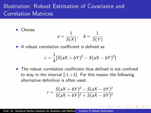
Illustration: Robust Estimation of Covariance andCorrelation Matrices
I Choose
a =1
S(X ), b =
1
S(Y )
I A robust correlation coefficient is defined as
c =1
4[S(aX + bY )2 − S(aX − bY )2]
I The robust correlation coefficient thus defined is not confinedto stay in the interval [-1,+1]. For this reason the followingalternative definition is often used:
r =S(aX + bY )2 − S(aX − bY )2
S(aX + bY )2 + S(aX − bY )2
Prof. Dr. Svetlozar Rachev Institute for Statistics and Mathematical Economics University of KarlsruheLecture 12 Robust Estimation

Illustration: Applications
I Robust regressions have been used to improve estimates in thearea of the market risk of a stock (beta) and of the factorloadings in a factor model.
I Martin and Simin propose a weighted least-squares estimatorwith data-dependent weights for estimating beta, referring tothis estimate as ”resistant beta”, and report that this beta isa superior predictor of future risk and return characteristicsthan the beta calculated using LS. The potentialdramatic difference between the LS beta and the resistant beta:
Prof. Dr. Svetlozar Rachev Institute for Statistics and Mathematical Economics University of KarlsruheLecture 12 Robust Estimation

Illustration: Applications
I Fama and French studies find that market capitalization (size)and book-to-market are important factors in explainingcross-sectional returns. These results are purely empiricallybased.
I The empirical evidence that size may be a factor that earns arisk premia was first reported by Banz.
I Knez and Ready reexamined the empirical evidence usingrobust regressions (the least-trimmed squares regression).First, they find that when 1% of the most extremeobservations are trimmed each month, the risk premia for thesize factor disappears.Second, the inverse relation between size and the risk premiano longer holds when the sample is trimmed.
Prof. Dr. Svetlozar Rachev Institute for Statistics and Mathematical Economics University of KarlsruheLecture 12 Robust Estimation

Final Remarks
I The required textbook is ”Financial Econometrics: FromBasics to Advanced Modeling Techniques”.
I Please read Chapter 12 for today’s lecture.
I All concepts explained are listed in page 428 of the textbook.
Prof. Dr. Svetlozar Rachev Institute for Statistics and Mathematical Economics University of KarlsruheLecture 12 Robust Estimation