Embed Size (px)
Citation preview

Lecture 13
Earth’s Free Oscillations

Earth’s Free Oscillations
Seismology and the Earth’s Deep Interior Surface Waves and Free Oscillations
Eigenmodes of a stringEigenmodes of a string
Geometry of a string underntension with fixed end points. Motions of the string excited
by any source comprise a weighted sum of the
eigenfunctions (which?).
Normal mode: all particles of the system move sinusoidally with the same frequency

Normal mode: stationary waves that are created from the constructive interference of body and surface waves circling the earth multiple times
Data - seismogramsMw ~9.2 2004 26 December, Sumatra
0 12108642
Time (s)
Time (h)

radial


6S4 30S12
http://icb.u-bourgogne.fr/nano/manapi/saviot/terre/index.en.html#
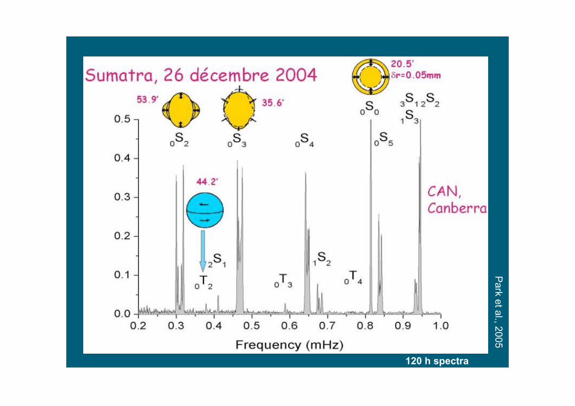
Park et al., 2005
120 h spectra

Free Oscillations - Spectra contain information about large scale
structure of Earth - Depend on broad averages of the Earth’s structural
parameters - Not affected by limitations of data coverage due to
uneven distribution of earthquakes and stations - Represents a quest to understand Earth’s intrinsic
vibrational spectrum - Provides a method for calculation of theoretical
seismograms - Intrinsic low pass filters of Earth’s structure

into two peaks in the data spectrum, which is not seenin the theoretical spectrum. Not shown here, butequally important in studying both Earth structureand earthquakes, is the ‘phase spectrum’. Examplesillustrating this are shown in later sections.
Normal mode studies represent the quest to revealand understand the Earth’s intrinsic vibrational spec-trum. However, this is a difficult quest, because it isonly at the very longest periods (!500 s, say) thatthere is the possibility of obtaining data of sufficientduration to make it possible to achieve the necessaryspectral resolution. Essentially, the modes attenuatebefore the many cycles necessary to establish a stand-ing wave pattern have elapsed. Thus, in manyobservational studies, over a wide range of frequen-cies, the normal mode representation has the role,primarily, of providing a method for the calculationof theoretical seismograms. Although observed spec-tra contain spectral peaks, the peaks are broadenedby the effects of attenuation in a path-dependentway. Thus, rather than making direct measurementson observed spectra, the analysis needs to be based oncomparisons between data and synthetic spectra, inorder to derive models able to give improved agree-ment between data and synthetics.
The use of normal mode theory as a method ofsynthesis extends well beyond the realm normallythought of as normal mode studies. For example, ithas become commonplace to calculate global bodywave theoretical seismograms by mode summation ina spherical model, to frequencies higher than100 mHz (10 s period). Typically, such calculationscan be done in seconds on an ordinary workstation,the time, of course, depending strongly upon theupper limit in frequency and on the number of sam-ples in the time series. The advantage of the method
is that all seismic phases are automatically included,with realistic time and amplitude relationships.Although the technique is limited (probably for theforeseeable future) to spherically symmetric models,the comparison of such synthetics with data providesa valuable tool for understanding the nature andpotential of the observations and for making mea-surements such as differences in timing between dataand synthetics, for use in tomography. Thus, theperiod range of applications of the normal moderepresentation extends from several thousand sec-onds to "5 s. In between these ends of the spectrumis an enormous range of applications: studies ofmodes per se, surface wave studies, analysis of over-tones, and long period body waves, each havingrelevance to areas such as source parameter estima-tion and tomography. Figure 2 shows an example ofsynthetic and data traces, illustrating this.
There are a number of excellent sources of infor-mation on normal modes theory and applications.The comprehensive monograph by Dahlen andTromp (1998) provides in-depth coverage of thematerial and an extensive bibliography. An earliermonograph by Lapwood and Usami (1981) containsmuch interesting and useful information, treated froma fundamental point of view, as well as historicalmaterial about early theoretical work and early obser-vations. A review by Takeuchi and Saito (1972) is agood source for the ordinary differential equations forspherical Earth models and methods of solution.Other reviews are by Gilbert (1980), Dziewonskiand Woodhouse (1983), and Woodhouse (1996). Areview of normal mode observations can be found inChapter 1.03. Because of this extensive literature wetend in this chapter to expand on some topics thathave not found their way into earlier reviews but arenevertheless of fundamental interest and utility.
1.02.2 Hamilton’s Principle andthe Equations of Motion
To a good approximation, except in the vicinity of anearthquake or explosion, seismic displacements aregoverned by the equations of elasticity. At long per-iods self-gravitation also plays an important role.Here we show how the equations of motion arisefrom Hamilton’s principle.
Consider a material which is initially in equili-brium under self-gravitation. Each particle of thematerial is labeled by Cartesian coordinates xi
(i¼ 1, 2, 3), representing its initial position. The
1.0 1.1 1.2 1.3 1.4 1.5 1.6 1.7Frequency (mHz)
0S6
3S21S4
0S72S3
1S5
2S4
4S1
0S8
3S3
2S5
1S6
0S9
1S0
1S7
2S6
5S1
4S2
0S10
Figure 1 Data (solid line) and PREM synthetic spectrum(dashed line) computed using normal mode summation, forthe vertical component recording at station ANMO followingthe great Sumatra event of 26 December 2004.
32 Earth’s Free Oscillations
Woodhouse & Deuss, 2007

Spherical Harmonics
- Angular solution to Laplace’s equation in spherical coordinates
- Wave propagation on the surface of a sphere - Can also be thought of as Fourier transformation
on a sphere - is a spherical harmonic function of degree l and
order m - is associated Legendre polynomial
Nu =Qd
kDT
⇠ 10
Pr =nk⇠ •
—2
f = 0
Y
m
l
(q,f) = Ne
imfP
m
l
(cosq)
5
Nu =Qd
kDT
⇠ 10
Pr =nk⇠ •
—2
f = 0
Y
m
l
(q,f) = Ne
imfP
m
l
(cosq)
5
Nu =Qd
kDT
⇠ 10
Pr =nk⇠ •
—2f = 0
5
Nu =Qd
kDT
⇠ 10
Pr =nk⇠ •
—2
f = 0
Y
m
l
(q,f) = Ne
imfP
m
l
(cosq)
5

Associated Legendre Polynomials
Nu =Qd
kDT
⇠ 10
Pr =nk⇠ •
—2
f = 0
Y
m
l
(q,f) = Ne
imfP
m
l
(cosq)
P
m
l
(x) =(�1)m
2
l
l!
(1� x
2)m/2
d
l+m
dx
l+m
(x2 �1)l
5

https://mysite.du.edu/~jcalvert/math/harmonic/harmonic.htm
m=0 m=/l m=l

48 CHAPTER 2. THE EARTH’S GRAVITATIONAL FIELD
Figure 2.14: Some spherical harmonics.
1. with increasing distance the lower order harmonics become increasingly dominant since thesignal from small-scale structure (large ’s and ’s) decays more rapidly. Recall that theperturbations of satellite orbits constrain the lower orders very accurately. The fine detailsat depth are difficult to discern at the surface of the Earth (or further out in space) owing tothis spatial attenuation.
2. Conversely, this complicates the downward continuation of from the Earth’s sur-face to a smaller radius, since this process introduces higher degree components in the so-lutions that are not constrained by data at the surface. This problem is important in thedownward continuation of the magnetic field to the core-mantle-boundary.

l = 16 m=0 l = 16 m=8
l = 16 m=16 http://geodynamics.usc.edu/~becker/teaching-sh.html

degree=6
−100−80−60−40−20020406080100
degree=50
−120−100−80−60−40−20020406080100120
l = 6 l = 50
Observed geoid

degree=6
−100−80−60−40−20020406080100
degree=50
−120−100−80−60−40−20020406080100120
l = 6
l = 50
Observed geoid
degree=7−31
−30
−20
−10
0
10
20
30l > 6

0"
500"
1000"
1500"
2000"
2500"
3000"
1" 3" 5" 7" 9" 11" 13" 15" 17" 19" 21" 23" 25" 27" 29" 31"
Series2"
Series1"
Degree
Pow
er
Observed geoid