Embed Size (px)
Citation preview
Lecture 13:Mapping Landmarks
CS 344R: Robotics
Benjamin Kuipers
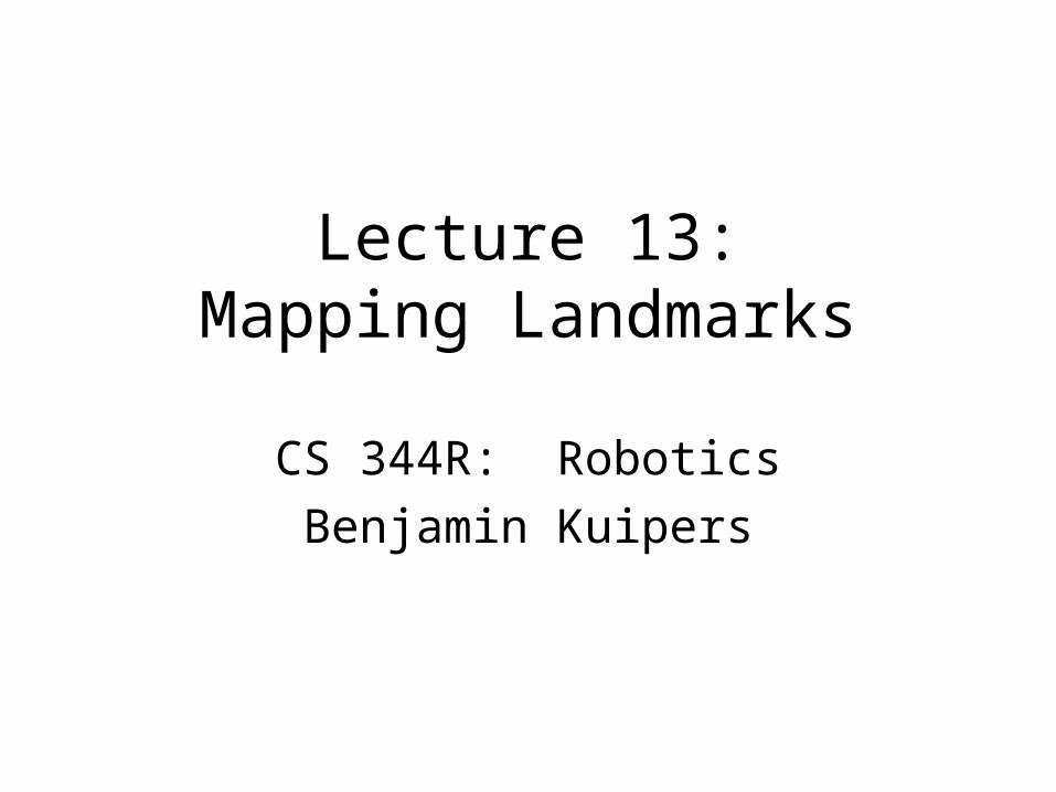
Landmark Map
• Locations and uncertainties of n landmarks, with respect to a specific frame of reference.– World frame: fixed origin point– Robot frame: origin at the robot
• Problem: how to combine new information with old to update the map.
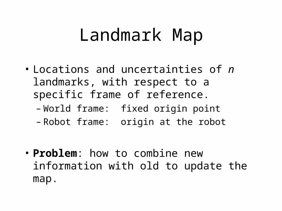
A Spatial Relationship is a Vector
• A spatial relationship holds between two poses: the position and orientation of one, in the frame of reference of the other.
€
xAB =
xAB
yAB
φAB
⎡
⎣
⎢ ⎢ ⎢
⎤
⎦
⎥ ⎥ ⎥
€
xAB = xAB yAB φAB[ ]T
A
B
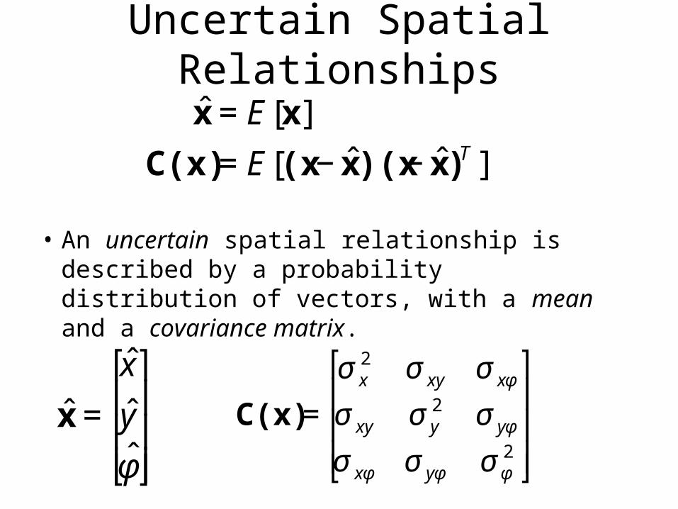
Uncertain Spatial Relationships
• An uncertain spatial relationship is described by a probability distribution of vectors, with a mean and a covariance matrix.€
ˆ x = E[x]
C(x) = E[(x − ˆ x )(x − ˆ x )T ]
€
ˆ x =
ˆ x
ˆ y ˆ φ
⎡
⎣
⎢ ⎢ ⎢
⎤
⎦
⎥ ⎥ ⎥
€
C(x) =
σ x2 σ xy σ xφ
σ xy σ y2 σ yφ
σ xφ σ yφ σ φ2
⎡
⎣
⎢ ⎢ ⎢
⎤
⎦
⎥ ⎥ ⎥

A Map with n Landmarks• Concatenate n vectors into one big state vector
• And one big 3n3n covariance matrix.
€
x =
x1
x2
M
xn
⎡
⎣
⎢ ⎢ ⎢ ⎢
⎤
⎦
⎥ ⎥ ⎥ ⎥
€
ˆ x =
ˆ x 1ˆ x 2M
ˆ x n
⎡
⎣
⎢ ⎢ ⎢ ⎢
⎤
⎦
⎥ ⎥ ⎥ ⎥
€
C(x) =
C(x1) C(x1,x2) L C(x1,xn )
C(x2,x1) C(x2) L C(x2,xn )
M M O M
C(xn,x1) C(xn,x2) L C(xn )
⎡
⎣
⎢ ⎢ ⎢ ⎢
⎤
⎦
⎥ ⎥ ⎥ ⎥
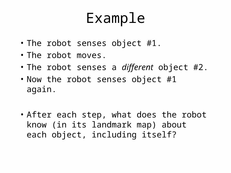
Example
• The robot senses object #1.
• The robot moves.
• The robot senses a different object #2.
• Now the robot senses object #1 again.
• After each step, what does the robot know (in its landmark map) about each object, including itself?
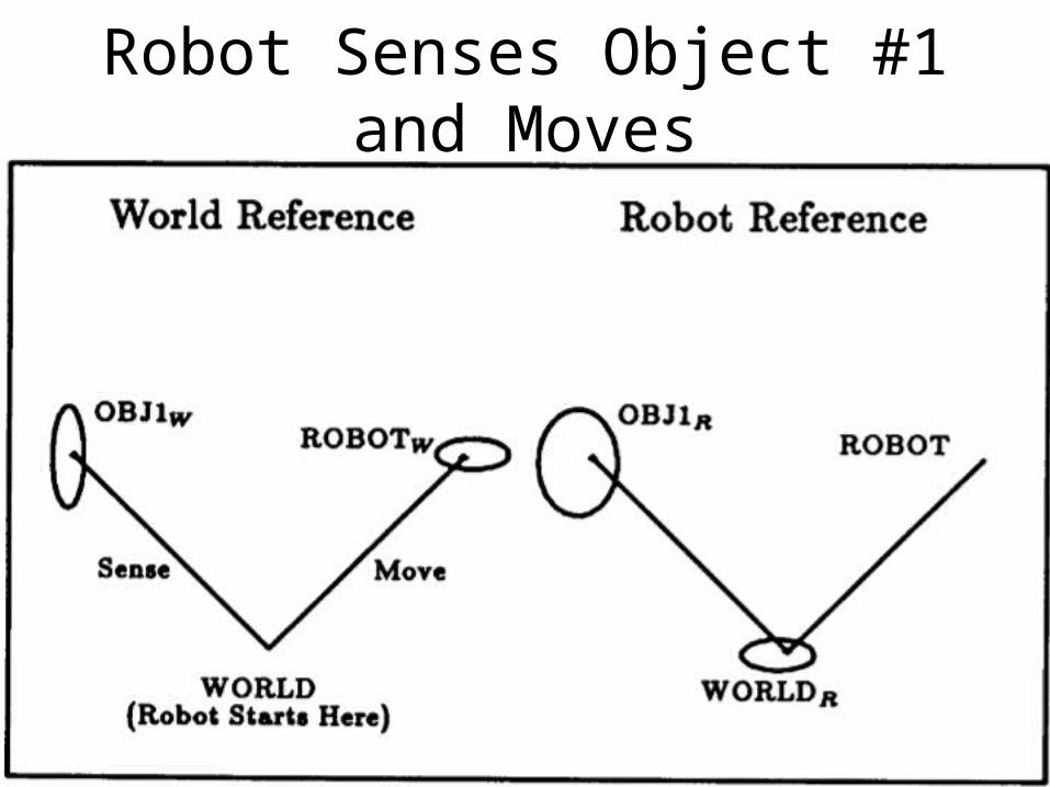
Robot Senses Object #1 and Moves
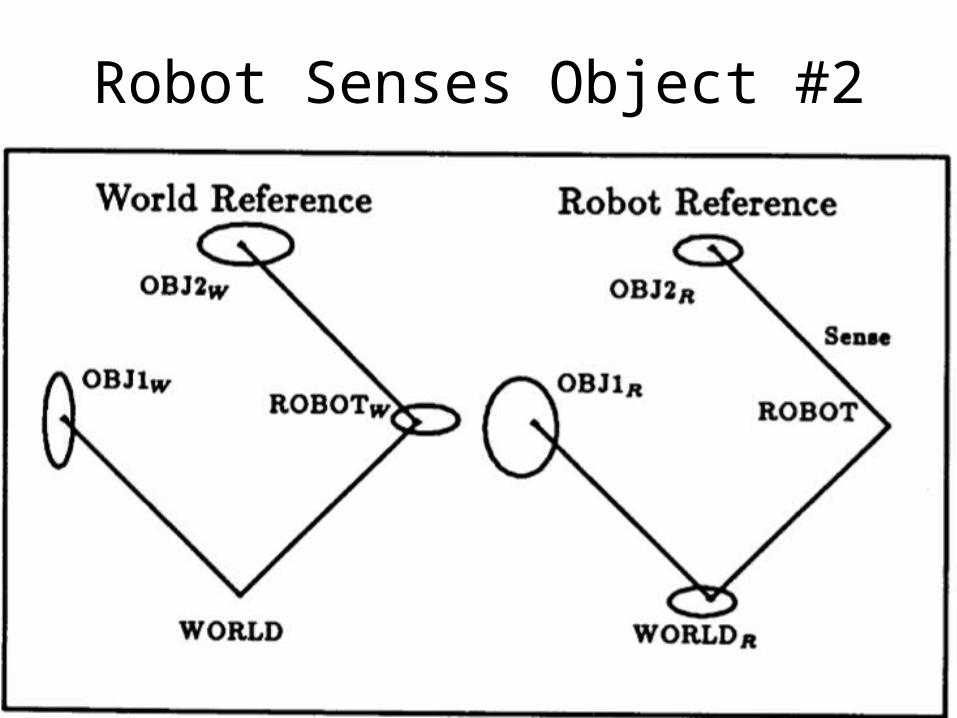
Robot Senses Object #2

Robot Senses Object #1 Again
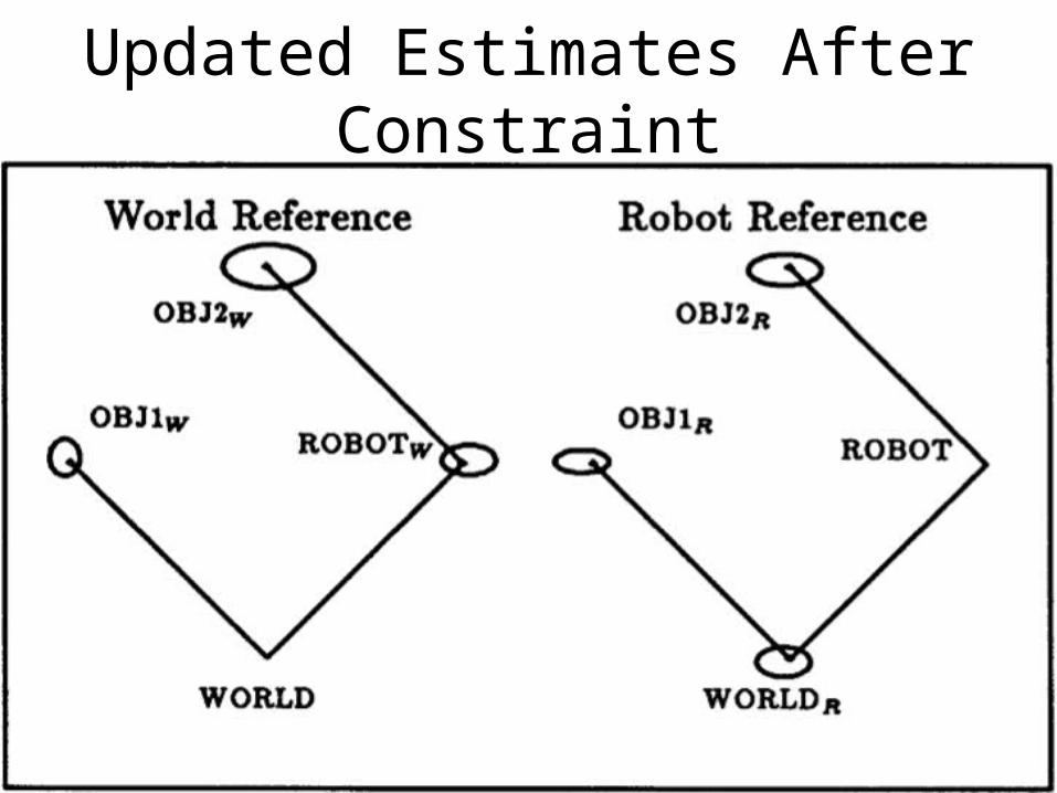
Updated Estimates After Constraint

Compounding
€
xAB = xAB yAB φAB[ ]T
€
xBC = xBC yBC φBC[ ]T

Compounding
€
xAB = xAB yAB φAB[ ]T
€
xBC = xBC yBC φBC[ ]T
€
xAC = xAC yAC φAC[ ]T
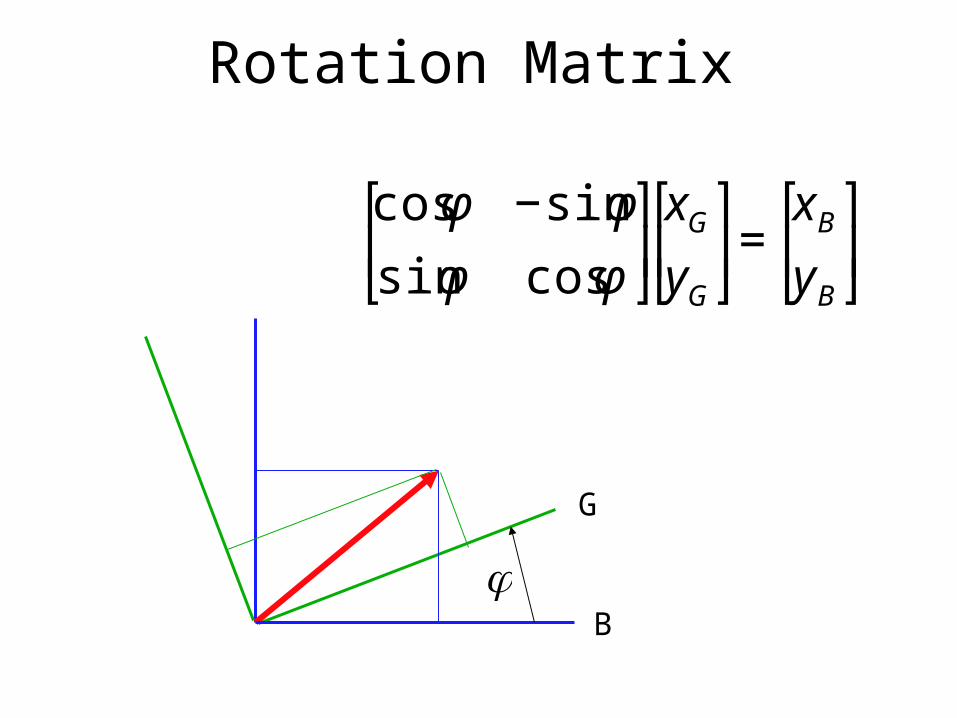
Rotation Matrix
€
cosφ −sinφ
sinφ cosφ
⎡
⎣ ⎢
⎤
⎦ ⎥xG
yG
⎡
⎣ ⎢
⎤
⎦ ⎥=
xB
yB
⎡
⎣ ⎢
⎤
⎦ ⎥
€
φB
G

Compounding
• Let xAB be the pose of object B in the frame of reference of A. (Sometimes written BA.)
• Given xAB and xBC, calculate xAC.
• Compute C(xAC) from C(xAB), C(xBC), and C(xAB,xBC).€
xAC = xAB ⊕ xBC =
xBC cosφAB − yBC sinφAB + xAB
xBC sinφAB + yBC cosφAB + yAB
φAB + φBC
⎡
⎣
⎢ ⎢ ⎢
⎤
⎦
⎥ ⎥ ⎥
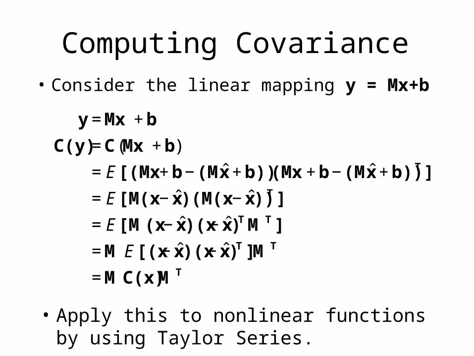
Computing Covariance
• Apply this to nonlinear functions by using Taylor Series.€
y = Mx + b
C(y) = C(Mx + b)
= E[(Mx + b − (Mˆ x + b)) (Mx + b − (Mˆ x + b))T ]
= E[M(x − ˆ x ) (M(x − ˆ x ))T ]
= E[M (x − ˆ x )(x − ˆ x )T MT ]
= M E[(x − ˆ x )(x − ˆ x )T ]MT
= MC(x)MT
• Consider the linear mapping y = Mx+b

Inverse Relationship
€
xAB = xAB yAB φAB[ ]T
€
xBA = xBA yBA φBA[ ]T
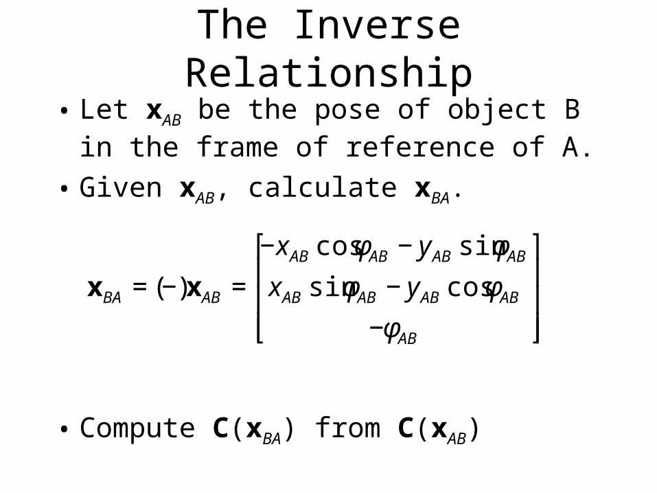
The Inverse Relationship
• Let xAB be the pose of object B in the frame of reference of A.
• Given xAB, calculate xBA.
• Compute C(xBA) from C(xAB)€
xBA = (−)xAB =
−xAB cosφAB − yAB sinφAB
xAB sinφAB − yAB cosφAB
−φAB
⎡
⎣
⎢ ⎢ ⎢
⎤
⎦
⎥ ⎥ ⎥

Composite Relationships• Compounding combines relationships head-
to-tail: xAC = xAB xBC
• Tail-to-tail combinations come from observing two things from the same point: xBC = (xAB) xAC
• Head-to-head combinations come from two observations of the same thing: xAC = xAB (xCB)
• They provide new relationships between their endpoints.
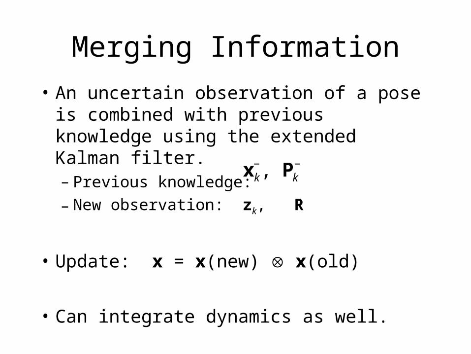
Merging Information
• An uncertain observation of a pose is combined with previous knowledge using the extended Kalman filter.– Previous knowledge:
– New observation: zk, R
• Update: x = x(new) x(old)
• Can integrate dynamics as well.
€
x k−, Pk
−
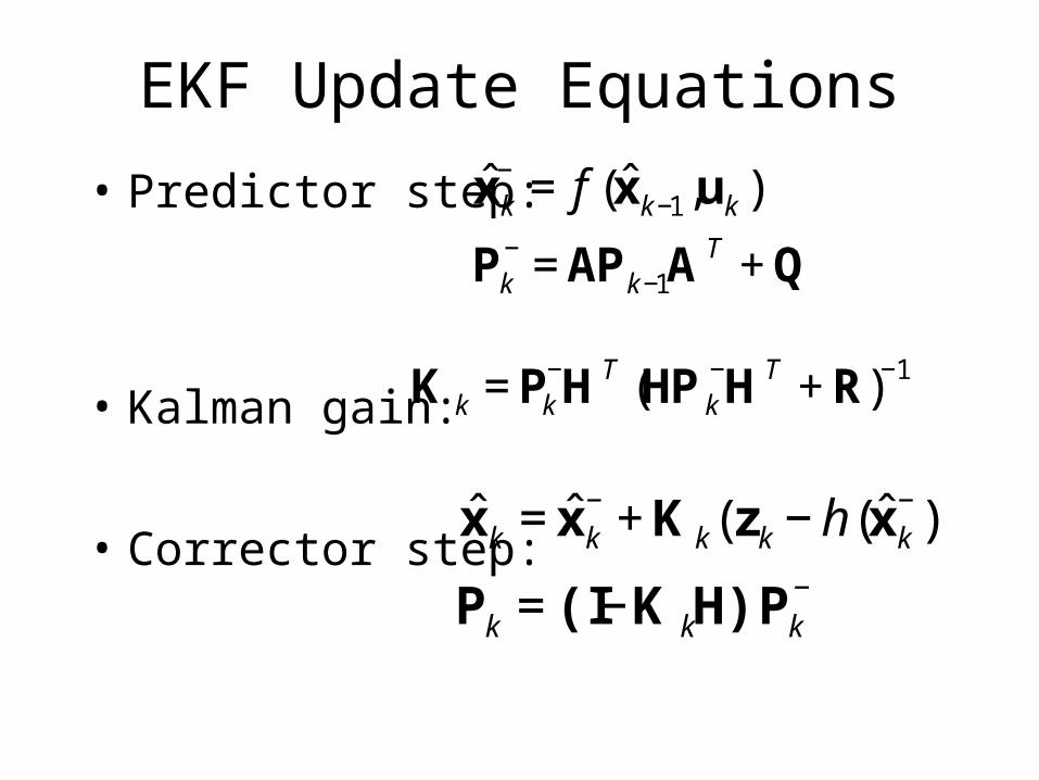
EKF Update Equations
• Predictor step:
• Kalman gain:
• Corrector step:
€
ˆ x k− =f (ˆ x k−1,uk)
€
Pk−=APk−1A
T +Q
€
K k =Pk−HT (HPk
−HT +R)−1
€
ˆ x k =ˆ x k−+Kk(zk−h(ˆ x k
−))
€
Pk =(I−K kH)Pk−
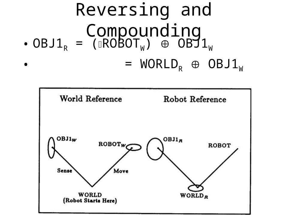
Reversing and Compounding• OBJ1R = (ROBOTW) OBJ1W
• = WORLDR OBJ1W
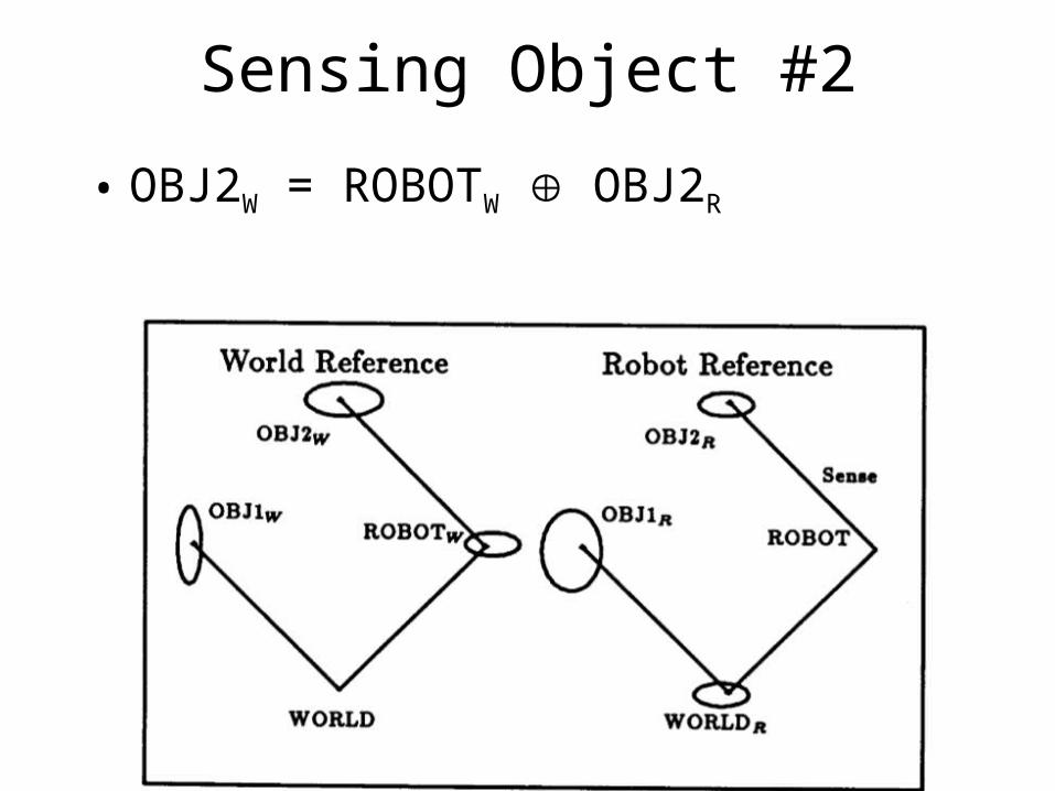
Sensing Object #2
• OBJ2W = ROBOTW OBJ2R
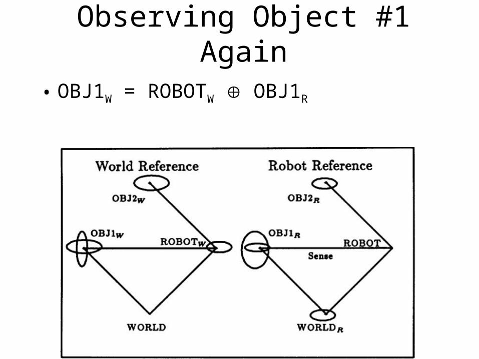
Observing Object #1 Again
• OBJ1W = ROBOTW OBJ1R
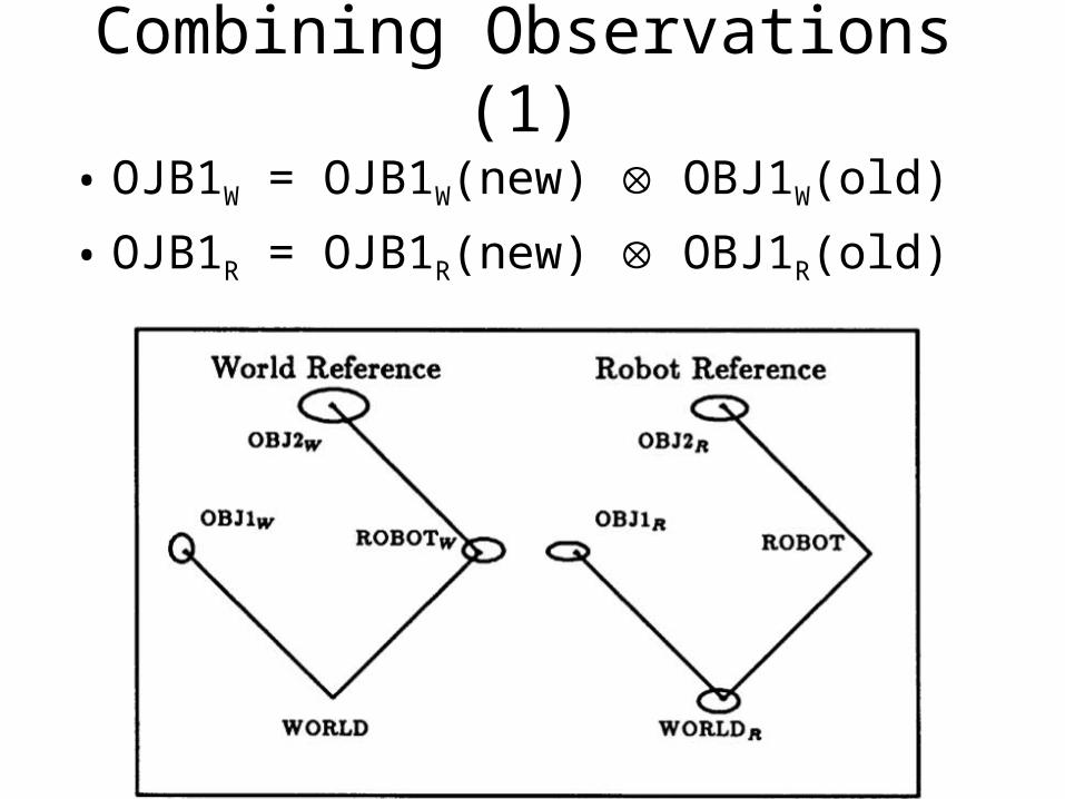
Combining Observations (1)
• OJB1W = OJB1W(new) OBJ1W(old)
• OJB1R = OJB1R(new) OBJ1R(old)
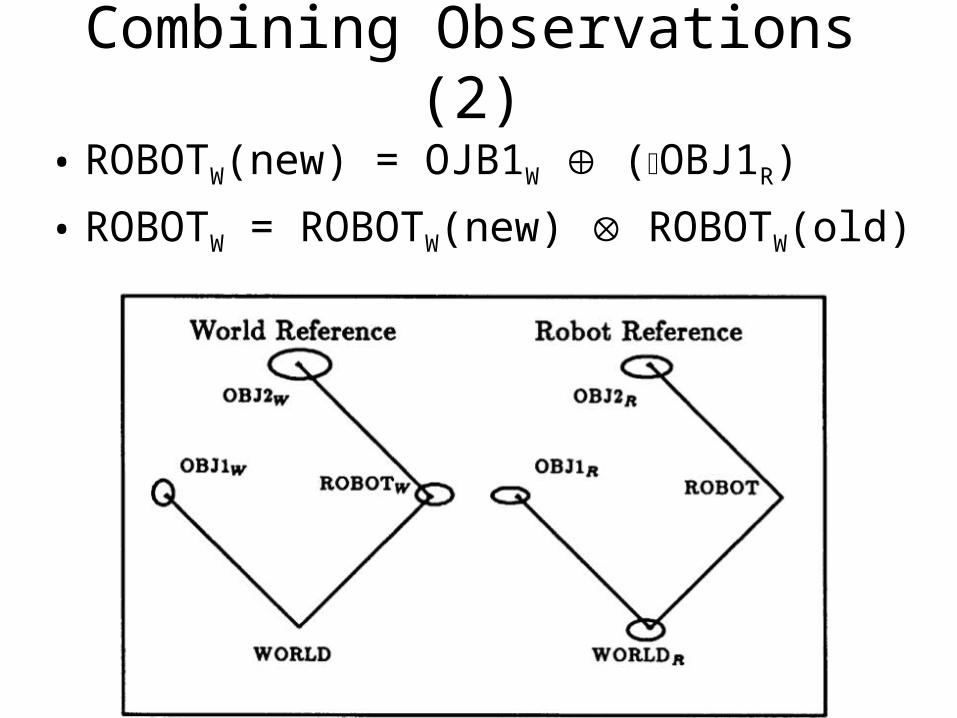
Combining Observations (2)
• ROBOTW(new) = OJB1W (OBJ1R)
• ROBOTW = ROBOTW(new) ROBOTW(old)
Useful for Feature-Based Maps
• We’ll see this again when we study FastSLAM.