Lecture 16 Unit Root Tests - Bauer College of Business · RS – EC2 - Lecture 16 4 • Note that an OLS estimation of , under a unit root, involves taking averages of the integrated

RS – EC2 - Lecture 16

1

1

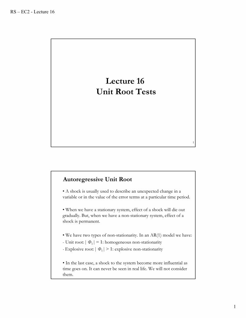
Lecture 16Unit Root Tests

• A shock is usually used to describe an unexpected change in a variable or in the value of the error terms at a particular time period.

• When we have a stationary system, effect of a shock will die out gradually. But, when we have a non-stationary system, effect of a shock is permanent.

• We have two types of non-stationarity. In an AR(1) model we have:

- Unit root: | Φ1 | = 1: homogeneous non-stationarity

- Explosive root: | Φ1 | > 1: explosive non-stationarity

• In the last case, a shock to the system become more influential as time goes on. It can never be seen in real life. We will not consider them.

Autoregressive Unit Root


2

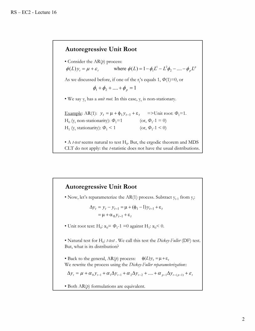
• Consider the AR(p) process:

As we discussed before, if one of the rj’s equals 1, Φ(1)=0, or

• We say yt has a unit root. In this case, yt is non-stationary.

Example: AR(1): =>Unit root: Φ1=1.

H0 (yt non-stationarity): Φ1=1 (or, Φ1-1 = 0)

H1 (yt stationarity): Φ1 < 1 (or, Φ1-1 < 0)

• A t-test seems natural to test H0. But, the ergodic theorem and MDS CLT do not apply: the t-statistic does not have the usual distributions.


pptt LLLLyL ....1)( where )( 2

211

1....21 p

11 ttt yy

• Now, let’s reparameterize the AR(1) process. Subtract yt-1 from yt:

• Unit root test: H0: α0= Φ1-1 =0 against H1: α0< 0.

• Natural test for H0: t-test . We call this test the Dickey-Fuller (DF) test. But, what is its distribution?

• Back to the general, AR(p) process:We rewrite the process using the Dickey-Fuller reparameterization::

• Both AR(p) formulations are equivalent.


.... )1(1221110 tptptttt yyyyy

tt

ttttt

y

yyyy

10

111 )1(

ttyL )(


3

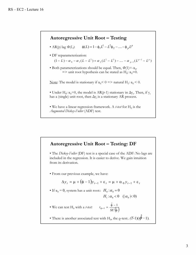
• AR(p) lag Φ(L):

• DF reparameterization:

• Both parameterizations should be equal. Then, Φ(1)=-α0.=> unit root hypothesis can be stated as H0: α0=0.

Note: The model is stationary if α0< 0 => natural H1: α0 < 0.

• Under H0: α0=0, the model is AR(p-1) stationary in Δyt. Then, if ythas a (single) unit root, then Δyt is a stationary AR process.

• We have a linear regression framework. A t-test for H0 is the Augmented Dickey-Fuller (ADF) test.

)(....)()()1( 11

322

210

ppp LLLLLLL

Autoregressive Unit Root – Testingp

p LLLL ....1)( 221

1

• The Dickey-Fuller (DF) test is a special case of the ADF: No lags are included in the regression. It is easier to derive. We gain intuition from its derivation.

• From our previous example, we have:

• If α0 = 0, system has a unit root::

• We can test H0 with a t-test:

• There is another associated test with H0, the ρ-test:. (T-1)( −1).

Autoregressive Unit Root – Testing: DF

ttttt yyy 1011

)0|(|0:

0:

001

00

H

H

ˆ1ˆ

1SE

t


4

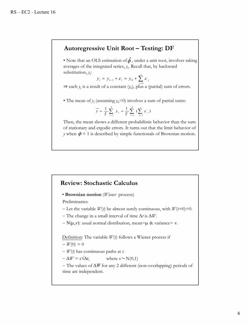
• Note that an OLS estimation of , under a unit root, involves taking averages of the integrated series, yt. Recall that, by backward substitution, yt:

⇒ each yt is a result of a constant (y0), plus a (partial) sum of errors.

• The mean of yt (assuming y0=0) involves a sum of partial sums:

Then, the mean shows a different probabilistic behavior than the sum of stationary and ergodic errors. It turns out that the limit behavior of y when ϕ = 1 is described by simple functionals of Brownian motion.


t

jjttt yyy

101

T

t

t

jj

T

tt T

yT

y1 11

)(11

• Brownian motion (Wiener process)

Preliminaries:

Let the variable W(t) be almost surely continuous, with W(t=0)=0.

The change in a small interval of time t is W.

(,v): usual normal distribution, mean= & variance= v.

Definition: The variable W(t) follows a Wiener process if

W(0) = 0

W(t) has continuous paths at t.

W = ε√t, where ε〜N(0,1)

The values of W for any 2 different (non-overlapping) periods of time are independent.

Review: Stochastic Calculus


5

9

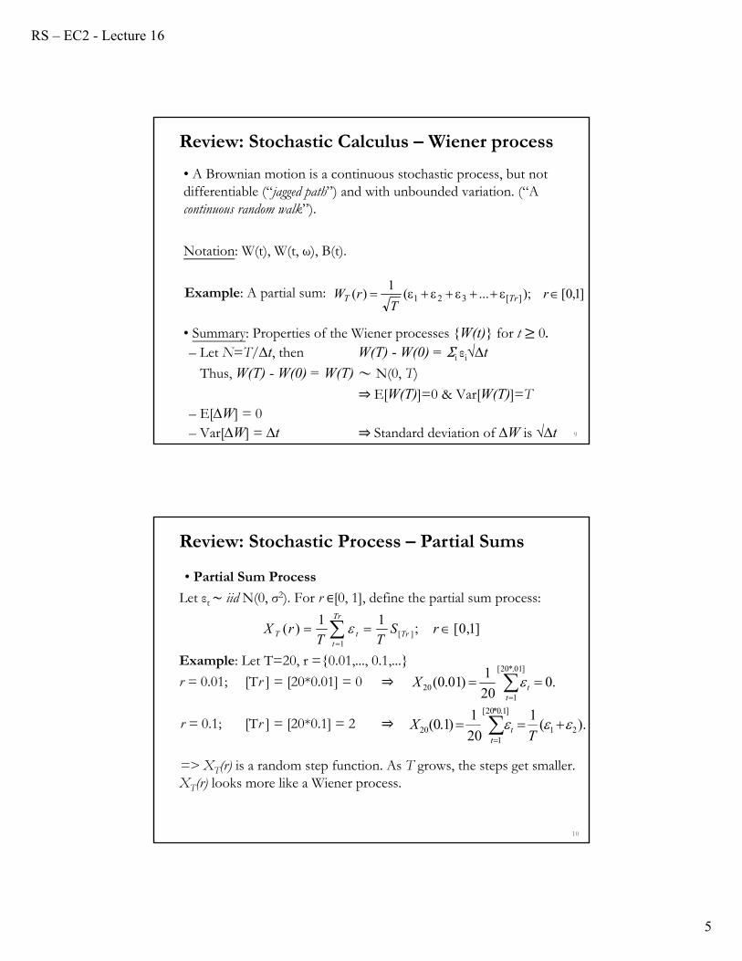
• A Brownian motion is a continuous stochastic process, but not differentiable (“jagged path”) and with unbounded variation. (“Acontinuous random walk”).

Notation: W(t), W(t, ω), B(t).

Example: A partial sum:

• Summary: Properties of the Wiener processes {W(t)} for t 0.– Let N=T/t, then W(T) - W(0) = Σi εi√t

Thus, W(T) - W(0) = W(T) 〜 N(0, T)

⇒E[W(T)]=0 & Var[W(T)]=T– E[W] = 0– Var[W] = t ⇒Standard deviation of W is √t

Review: Stochastic Calculus – Wiener process

]1,0[);...(1

)( ][321 rT

rW TrT

10

• Partial Sum Process

Let εt ∼ iid N(0, σ2). For r ∈[0, 1], define the partial sum process:

Example: Let T=20, r ={0.01,..., 0.1,...}

r = 0.01; [Tr ] = [20*0.01] = 0 ⇒

r = 0.1; [Tr ] = [20*0.1] = 2 ⇒

=> XT(r) is a random step function. As T grows, the steps get smaller. XT(r) looks more like a Wiener process.

Review: Stochastic Process – Partial Sums

]1,0[;11

)( ][1

rSTT

rX Tr

Tr

ttT

.020

1)01.0(

]01.*20[

120

ttX

).(1

20

1)1.0( 21

]1.0*20[

120

TX

tt


6

11

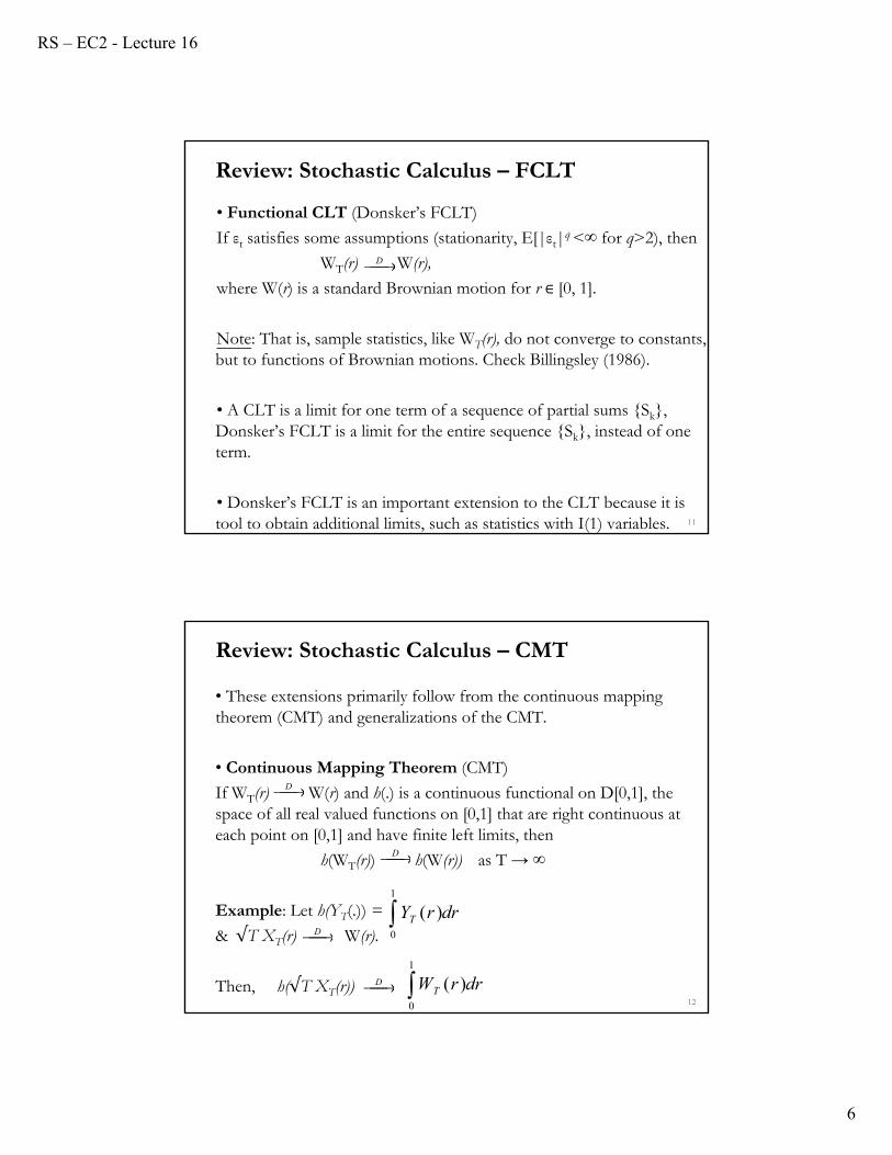
• Functional CLT (Donsker’s FCLT)

If εt satisfies some assumptions (stationarity, E[|εt|q <∞ for q>2), then

WT(r) W(r),

where W(r) is a standard Brownian motion for r ∈ [0, 1].

Note: That is, sample statistics, like WT(r), do not converge to constants, but to functions of Brownian motions. Check Billingsley (1986).

• A CLT is a limit for one term of a sequence of partial sums {Sk}, Donsker’s FCLT is a limit for the entire sequence {Sk}, instead of one term.

• Donsker’s FCLT is an important extension to the CLT because it is tool to obtain additional limits, such as statistics with I(1) variables.

Review: Stochastic Calculus – FCLT

D

12

• These extensions primarily follow from the continuous mapping theorem (CMT) and generalizations of the CMT.

• Continuous Mapping Theorem (CMT)

If WT(r) W(r) and h(.) is a continuous functional on D[0,1], the space of all real valued functions on [0,1] that are right continuous at each point on [0,1] and have finite left limits, then

h(WT(r)) h(W(r)) as T → ∞

Example: Let h(YT(.)) =

& √T XT(r) W(r).

Then, h(√T XT(r))

Review: Stochastic Calculus – CMT

D

D

drrYT1

0

)(

drrWT1

0

)(D

D


7

13

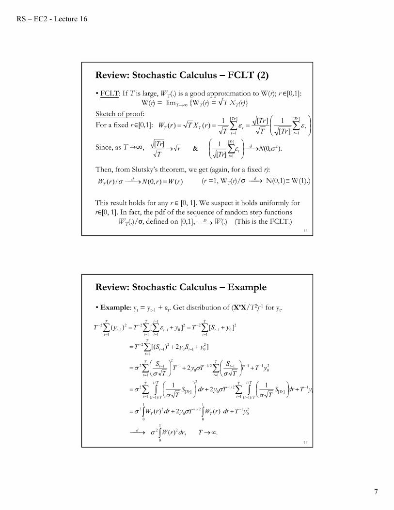
• FCLT: If T is large, WT(.) is a good approximation to W(r); r ∈[0,1]: W(r) = limT→∞ {WT(r) = √T XT(r)}

Sketch of proof:

For a fixed r ∈[0,1]:

Since, as T →∞,

Then, from Slutsky’s theorem, we get (again, for a fixed r):

(r =1, WT(r)/σ N(0,1)≡ W(1).)

This result holds for any r ∈ [0, 1]. We suspect it holds uniformly for r∈[0, 1]. In fact, the pdf of the sequence of random step functions

WT(.)/σ,defined on [0,1], W(.) (This is the FCLT.)

Review: Stochastic Calculus – FCLT (2)

][

1

][

1 ][

1][1)()(

Tr

tt

Tr

ttTT

TrT

Tr

TrXTrW

).,0(][

1&

][ 2][

1

NTr

rT

Tr dTr

tt

)(),0(/)( rWrNrW dT d

D

14

• Example: yt = yt-1 + εt. Get distribution of (X’X/T2)-1 for yt.

Review: Stochastic Calculus – Example

1

0

22

20

11

0

2/10

1

0

22

20

1

1

/

/)1(

][2/1

01

/

/)1(

2

][2

20

1

1

112/10

1

1

2

12

1

2010

21

2

1

201

2

1

21

10

2

1

21

2

.,)(

)(2)(

12

1

2

]2)[(

][][)(

TdrrW

yTdrrWTydrrW

yTdrST

TydrST

yTTT

STyT

T

S

ySyST

ySTyTyT

d

TT

T

t

Tt

Tt

Tr

T

t

Tt

Tt

Tr

T

t

tT

t

t

T

ttt

T

tt

T

t

t

iit

T

tt


8

15

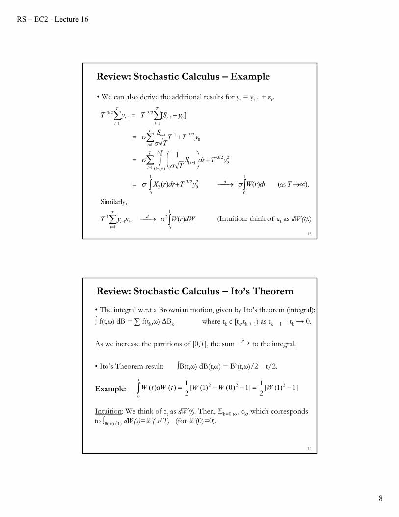
• We can also derive the additional results for yt = yt-1 + εt.

Review: Stochastic Calculus – Example

1

0

2

111

1

1

0

20

2/31

0

20

2/3

1

/

/)1(

][

02/31

1

1

101

2/3

11

2/3

)(

).()()(

1

][

dWrWyT

TdrrWyTdrrX

yTdrST

yTTT

S

ySTyT

dT

ttt

dT

T

t

Tt

Tt

Tr

T

t

t

T

tt

T

tt

Similarly,

as

(Intuition: think of εt as dW(t).)

16

• The integral w.r.t a Brownian motion, given by Ito’s theorem (integral):

∫ f(t,ω) dB = ∑ f(tk,ω) ∆Bk where tk є [tk,tk + 1) as tk + 1 – tk → 0.

As we increase the partitions of [0,T], the sum to the integral.

• Ito’s Theorem result: ∫B(t,ω) dB(t,ω) = B2(t,ω)/2 – t/2.

Example:

Intuition: We think of εt as dW(t). Then, Σk=0 to t εk, which corresponds to ∫0to(t/T) dW(s)=W( s/T) (for W(0)=0).

Review: Stochastic Calculus – Ito’s Theorem

p

]1)1([2

1]1)0()1([

2

1)()( 222

1

0

WWWtdWtW


9

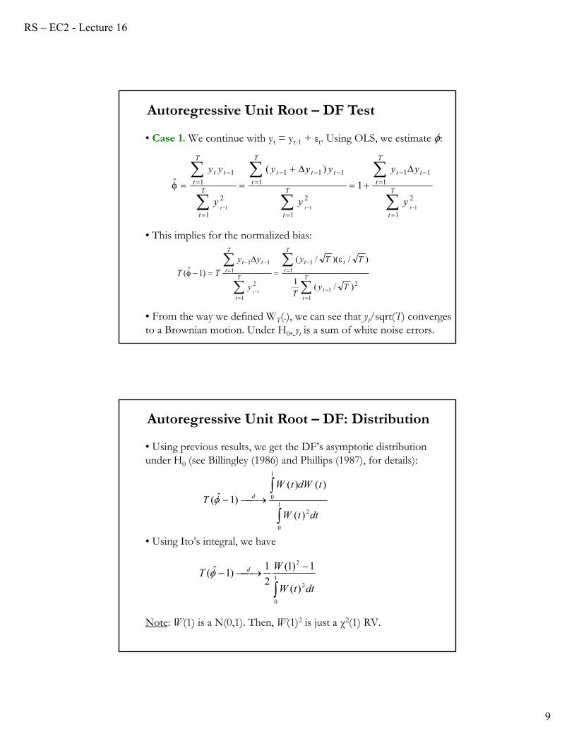
• Case 1. We continue with yt = yt-1 + εt. Using OLS, we estimate :

• This implies for the normalized bias:

• From the way we defined WT(.), we can see that yt/sqrt(T) converges to a Brownian motion. Under H0, yt is a sum of white noise errors.

Autoregressive Unit Root – DF Test

T

t

T

ttt

T

t

T

tttt

T

t

T

ttt

ttty

yy

y

yyy

y

yy

1

2

111

1

2

1111

1

2

11

111

1

)(ˆ

T

tt

T

ttt

T

t

T

ttt

TyT

TTy

y

yy

TT

t

1

21

11

1

2

111

)/(1

)/)(/(

)1ˆ(

1

• Using previous results, we get the DF’s asymptotic distribution under H0 (see Billingley (1986) and Phillips (1987), for details):

• Using Ito’s integral, we have

Note: W(1) is a N(0,1). Then, W(1)2 is just a χ2(1) RV.

dttW

tdWtW

T d

1

0

2

1

0

)(

)()(

)1ˆ(

dttW

WT d

1

0

2

2

)(

1)1(

2

1)1ˆ(

Autoregressive Unit Root – DF: Distribution


10

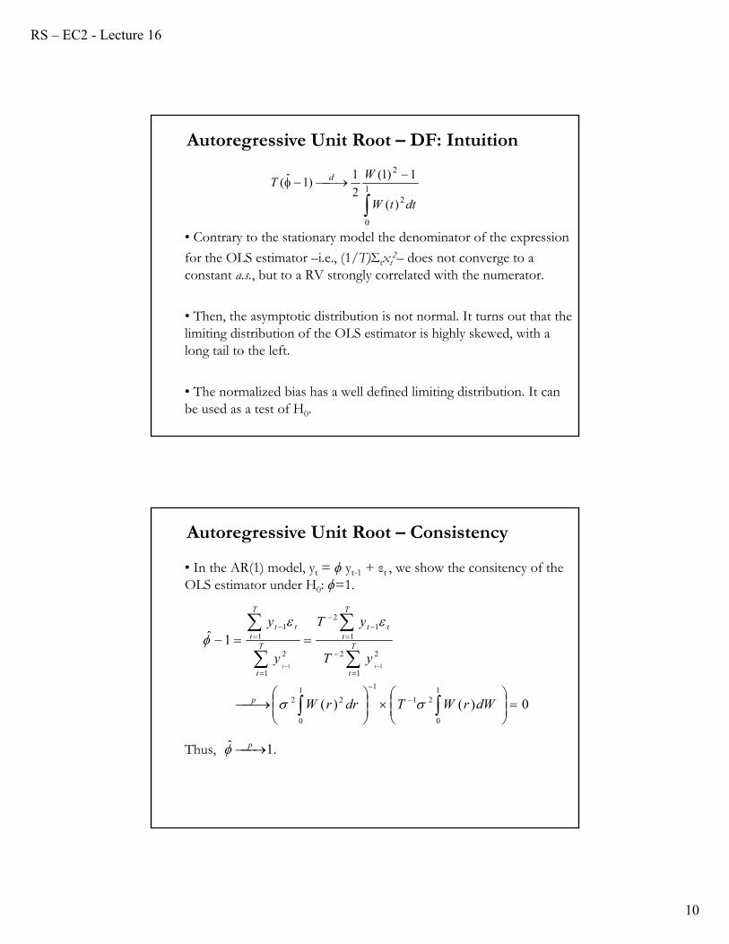
• Contrary to the stationary model the denominator of the expression

for the OLS estimator –i.e., (1/T)Σtxt2– does not converge to a

constant a.s., but to a RV strongly correlated with the numerator.

• Then, the asymptotic distribution is not normal. It turns out that the limiting distribution of the OLS estimator is highly skewed, with a long tail to the left.

• The normalized bias has a well defined limiting distribution. It can be used as a test of H0.

dttW

WT d

1

0

2

2

)(

1)1(

2

1)1ˆ(

Autoregressive Unit Root – DF: Intuition

• In the AR(1) model, yt = ϕ yt-1 + εt , we show the consitency of the OLS estimator under H0: ϕ=1.

Thus, .

Autoregressive Unit Root – Consistency

1ˆ p

0)()(

1ˆ

1

0

21

11

0

22

1

22

11

2

1

2

11

11

dWrWTdrrW

yT

yT

y

y

p

T

t

T

ttt

T

t

T

ttt

tt


11

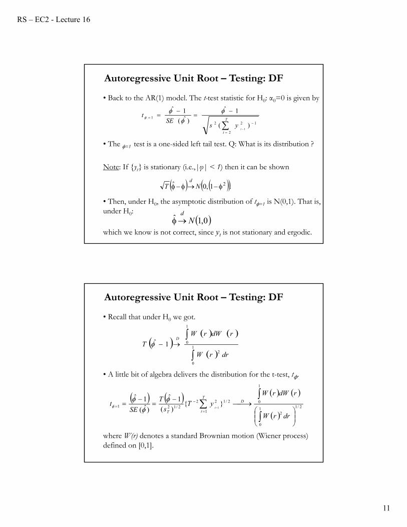
• Back to the AR(1) model. The t-test statistic for H0: α0=0 is given by

• The =1 test is a one-sided left tail test. Q: What is its distribution ?

Note: If {yt} is stationary (i.e.,|φ| < 1) then it can be shown

• Then, under H0, the asymptotic distribution of t=1 is N(0,1). That is, under H0:

which we know is not correct, since yt is not stationary and ergodic.


.1,0ˆ 2 NTd

T

tt

ysSE

t

2

122

1

)(

1ˆ

)ˆ(

1ˆ

1

0,1ˆ Nd

• Recall that under H0 we got.

• A little bit of algebra delivers the distribution for the t-test, tϕ.

where W(r) denotes a standard Brownian motion (Wiener process) defined on [0,1].


1

0

2

1

01ˆ

drrW

rdWrW

TD

2/11

0

2

1

0

1

2/1222/121 }{

)(

1ˆ

)ˆ(

1ˆ1

drrW

rdWrW

yTs

T

SEt D

T

tTt


12

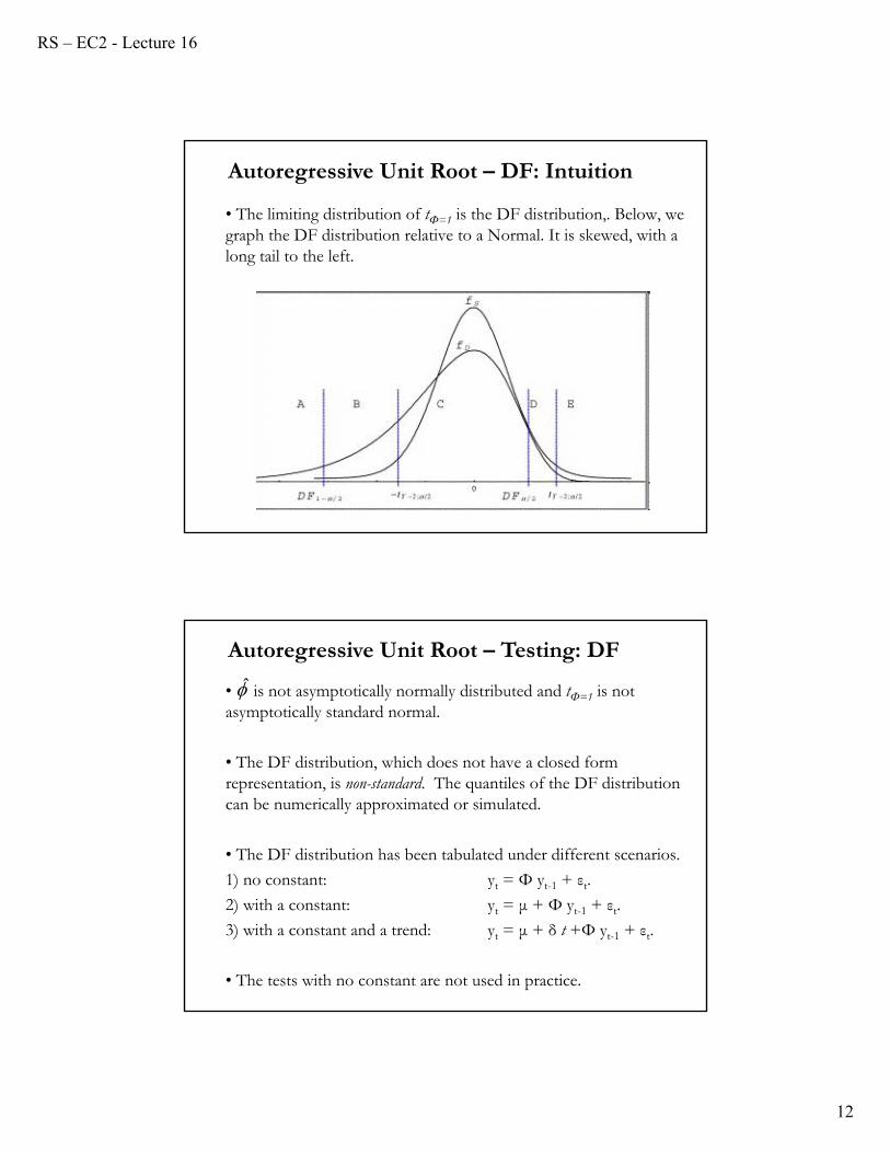
• The limiting distribution of tФ=1 is the DF distribution,. Below, we graph the DF distribution relative to a Normal. It is skewed, with a long tail to the left.

Autoregressive Unit Root – DF: Intuition

• is not asymptotically normally distributed and tФ=1 is not asymptotically standard normal.

• The DF distribution, which does not have a closed form representation, is non-standard. The quantiles of the DF distribution can be numerically approximated or simulated.

• The DF distribution has been tabulated under different scenarios.

1) no constant: yt = Φ yt-1 + εt.

2) with a constant: yt = μ + Φ yt-1 + εt.

3) with a constant and a trend: yt = μ + δ t +Φ yt-1 + εt.

• The tests with no constant are not used in practice.



13

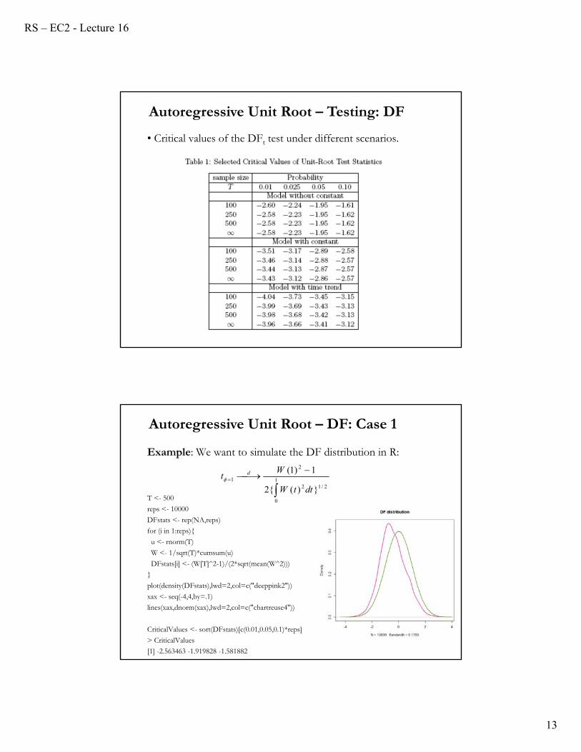
• Critical values of the DFt test under different scenarios.


Example: We want to simulate the DF distribution in R:

T <- 500

reps <- 10000

DFstats <- rep(NA,reps)

for (i in 1:reps){

u <- rnorm(T)

W <- 1/sqrt(T)*cumsum(u)

DFstats[i] <- (W[T]^2-1)/(2*sqrt(mean(W^2)))

}

plot(density(DFstats),lwd=2,col=c("deeppink2"))

xax <- seq(-4,4,by=.1)

lines(xax,dnorm(xax),lwd=2,col=c("chartreuse4"))

CriticalValues <- sort(DFstats)[c(0.01,0.05,0.1)*reps]

> CriticalValues

[1] -2.563463 -1.919828 -1.581882

2/11

0

2

2

1

})({2

1)1(

dttW

Wt d

Autoregressive Unit Root – DF: Case 1


14

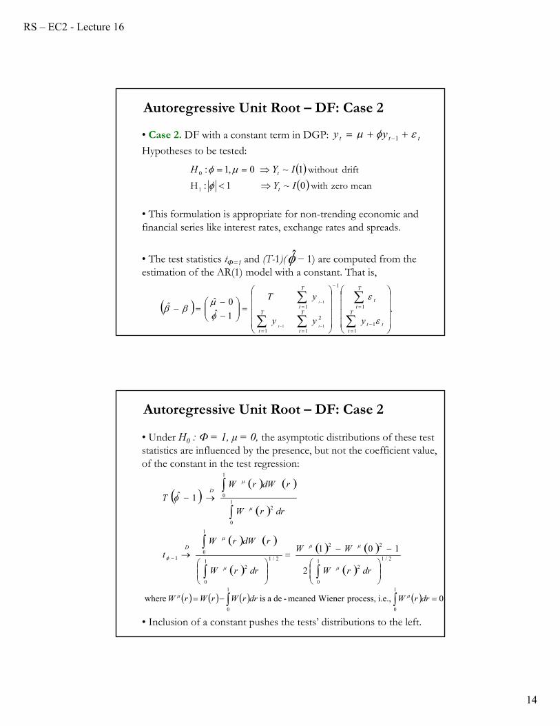
• Case 2. DF with a constant term in DGP:

Hypotheses to be tested:

• This formulation is appropriate for non-trending economic and financial series like interest rates, exchange rates and spreads.

• The test statistics tФ=1 and (T-1)( − 1) are computed from the estimation of the AR(1) model with a constant. That is,


ttt yy 1

mean zero with H

driftwithout

1 0~1:

1~0,1:0

IY

IYH

t

t

.1ˆ0ˆˆ

11

1

1

1

2

1

1

11

1

T

ttt

T

tt

T

t

T

t

T

t

yyy

yT

tt

t

• Under H0 : Ф = 1, μ = 0, the asymptotic distributions of these test statistics are influenced by the presence, but not the coefficient value, of the constant in the test regression:

• Inclusion of a constant pushes the tests’ distributions to the left.


2/11

0

2

22

2/11

0

2

1

01

1

0

2

1

0

2

101

1ˆ

drrW

WW

drrW

rdWrW

t

drrW

rdWrW

T

D

D

0 i.e., process, Wiener meaned-de a is where1

0

1

0

drrWdrrWrWrW


15

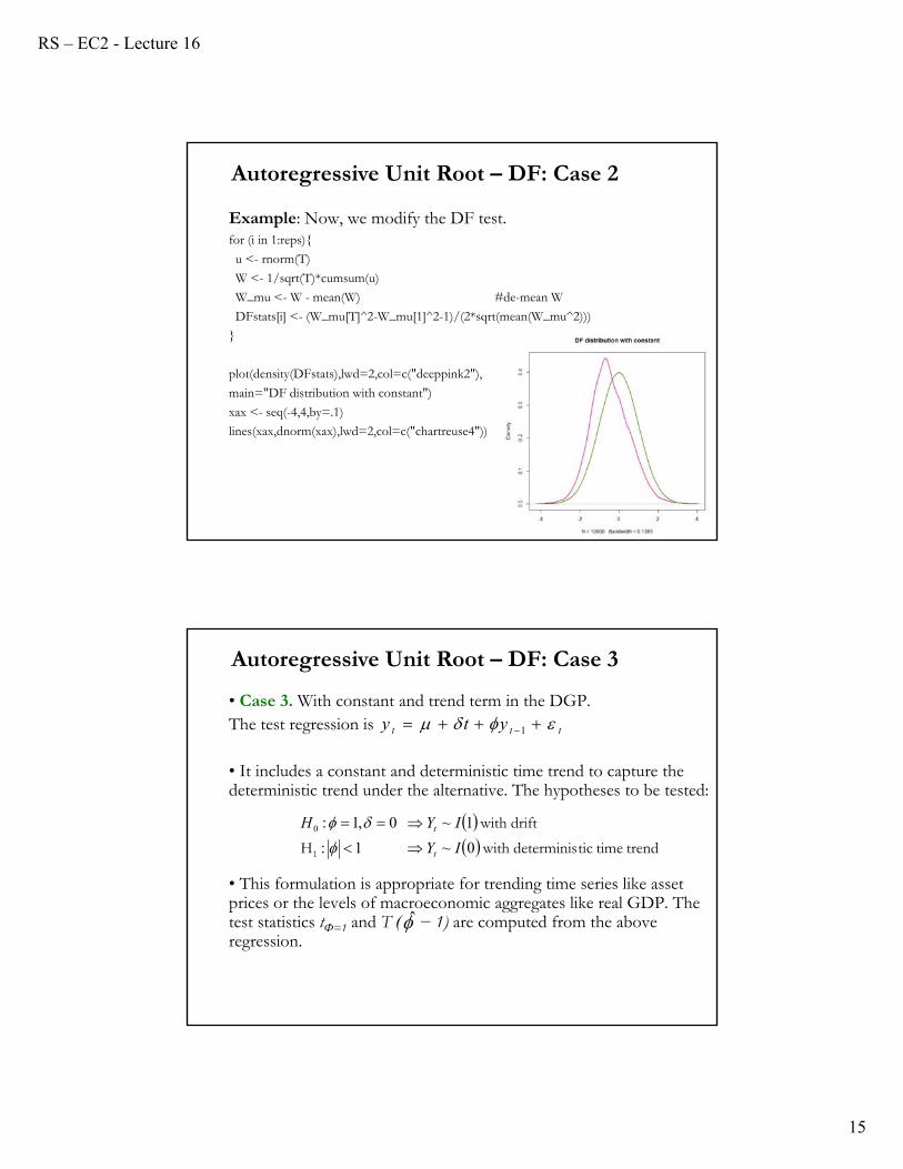
Example: Now, we modify the DF test.for (i in 1:reps){

u <- rnorm(T)


W_mu <- W - mean(W) #de-mean W

DFstats[i] <- (W_mu[T]^2-W_mu[1]^2-1)/(2*sqrt(mean(W_mu^2)))

}

plot(density(DFstats),lwd=2,col=c("deeppink2"),

main="DF distribution with constant")

xax <- seq(-4,4,by=.1)

lines(xax,dnorm(xax),lwd=2,col=c("chartreuse4"))


• Case 3. With constant and trend term in the DGP.The test regression is

• It includes a constant and deterministic time trend to capture the deterministic trend under the alternative. The hypotheses to be tested:

• This formulation is appropriate for trending time series like asset prices or the levels of macroeconomic aggregates like real GDP. The test statistics tФ=1 and T ( − 1) are computed from the above regression.


ttt yty 1

trend time ticdeterminis with H

drift with

1 0~1:

1~0,1:0

IY

IYH

t

t


16

• Again, under H0 : Ф = 1, δ = 0, the asymptotic distributions of both test statistics are influenced by the presence of the constant and time trend in the test regression. Now, we have:


2/11

0

2

22

2/11

0

2

1

01

1

0

2

1

0

2

101

1ˆ1

drrW

WW

drrW

rdWrW

t

drrW

rdWrW

T

d

d

process.Wiener trended-de& meaned-dea

is where 1

0

1

0

)612()64( dsssWrdssWrrWrW

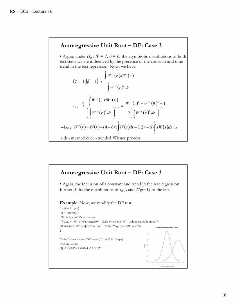
• Again, the inclusion of a constant and trend in the test regression further shifts the distributions of tФ=1 and T( −1) to the left.

Example: Now, we modify the DF test.for (i in 1:reps){

u <- rnorm(T)


W_tau <- W - (4-6*s)*mean(W) - (12*s-6)*mean(s*W) #de-mean & de-trend W

DFstats[i] <- (W_tau[T]^2-W_tau[1]^2-1)/(2*sqrt(mean(W_tau^2)))

}

CriticalValues <- sort(DFstats)[c(0.01,0.05,0.1)*reps]

>CriticalValues

[1] -3.930855 -3.390544 -3.118117



17

• Which version of the three main variations of the test should be used is not a minor issue. The decision has implications for the size and the power of the unit root test.

• For example, an incorrect exclusion of the time trend term leads to bias in the coefficient estimate for Φ, leading to size distortions and reductions in power.

• Since the normalized bias (T1)( − 1) has a well defined limiting distribution that does not depend on nuisance parameters it can also be used as a test statistic for the null hypothesis H0 : Ф = 1.

Autoregressive Unit Root – DF: Remarks

• Back to the general, AR(p) process. We can rewrite the equation as the Dickey-Fuller reparameterization:

• The model is stationary if α0< 0 => natural H1: α0 < 0.

• Under H0: α0=0, the model is AR(p-1) stationary in Δyt. Then, if yt

has a (single) unit root, then Δyt is a stationary AR process.

• The t-test for H0 from OLS estimation is the Augmented Dickey-Fuller (ADF) test.

• Similar situation as the DF test, we have a non-normal distribution.

Autoregressive Unit Root – Testing: ADF

.... )1(1221110 tptptttt yyyyy


18

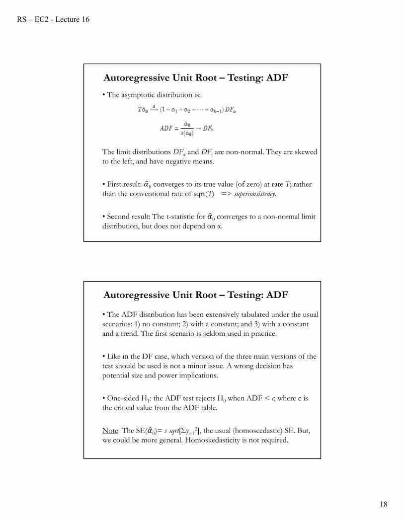
• The asymptotic distribution is:

The limit distributions DFα and DFt are non-normal. They are skewed to the left, and have negative means.

• First result: 0 converges to its true value (of zero) at rate T; rather than the conventional rate of sqrt(T) => superconsistency.

• Second result: The t-statistic for 0 converges to a non-normal limit distribution, but does not depend on α.


• The ADF distribution has been extensively tabulated under the usual scenarios: 1) no constant; 2) with a constant; and 3) with a constant and a trend. The first scenario is seldom used in practice.

• Like in the DF case, which version of the three main versions of the test should be used is not a minor issue. A wrong decision has potential size and power implications.

• One-sided H1: the ADF test rejects H0 when ADF < c; where c is the critical value from the ADF table.

Note: The SE( 0)= s sqrt[Σyt-12], the usual (homoscedastic) SE. But,

we could be more general. Homoskedasticity is not required.



19

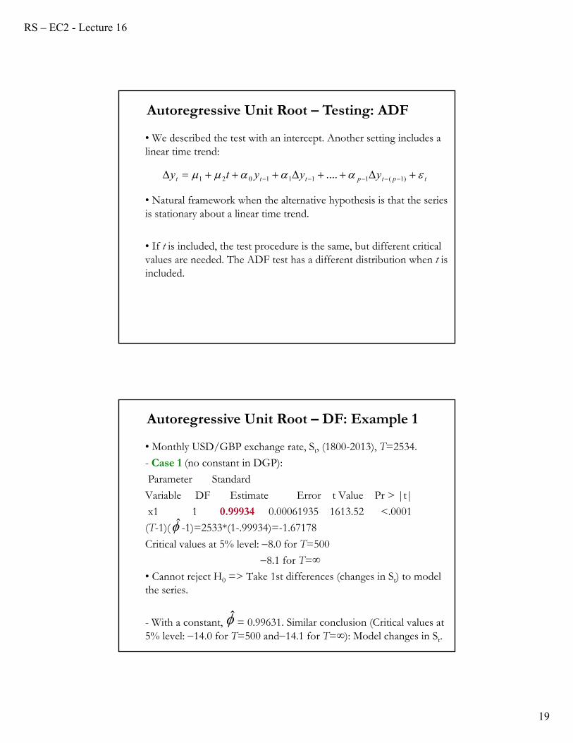
• We described the test with an intercept. Another setting includes a linear time trend:

• Natural framework when the alternative hypothesis is that the series is stationary about a linear time trend.

• If t is included, the test procedure is the same, but different critical values are needed. The ADF test has a different distribution when t is included.


.... )1(1111021 tptpttt yyyty

• Monthly USD/GBP exchange rate, St, (1800-2013), T=2534.

- Case 1 (no constant in DGP):

Parameter Standard

Variable DF Estimate Error t Value Pr > |t|

x1 1 0.99934 0.00061935 1613.52 <.0001

(T-1)( -1)=2533*(1-.99934)=-1.67178

Critical values at 5% level: 8.0 for T=500

8.1 for T=∞

• Cannot reject H0 => Take 1st differences (changes in St) to model the series.

- With a constant, = 0.99631. Similar conclusion (Critical values at 5% level: 14.0 for T=500 and14.1 for T=∞): Model changes in St.

Autoregressive Unit Root – DF: Example 1


20

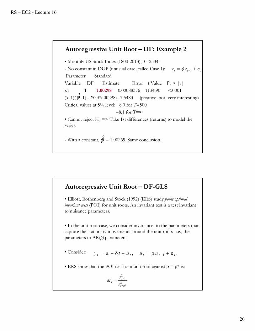
• Monthly US Stock Index (1800-2013), T=2534.

- No constant in DGP (unusual case, called Case 1):

Parameter Standard

Variable DF Estimate Error t Value Pr > |t|

x1 1 1.00298 0.00088376 1134.90 <.0001

(T-1)( -1)=2533*(.00298)=7.5483 (positive, not very interesting)

Critical values at 5% level: 8.0 for T=500

8.1 for T=∞

• Cannot reject H0 => Take 1st differences (returns) to model the series.

- With a constant, = 1.00269. Same conclusion.

Autoregressive Unit Root – DF: Example 2

ttt yy 1

• Elliott, Rothenberg and Stock (1992) (ERS) study point optimal invariant tests (POI) for unit roots. An invariant test is a test invariant to nuisance parameters.

• In the unit root case, we consider invariance to the parameters that capture the stationary movements around the unit roots -i.e., the parameters to AR(p) parameters.

• Consider:

• ERS show that the POI test for a unit root against ρ = ρ* is:

Autoregressive Unit Root – DF-GLS

., 1 ttttt uuuty

2*

21

s

sMT


21

•

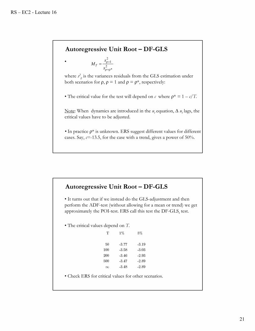
where s2ρ is the variances residuals from the GLS estimation under

both scenarios for ρ, ρ = 1 and ρ = ρ*, respectively:

• The critical value for the test will depend on c where ρ* = 1 – c/T.

Note: When dynamics are introduced in the ut equation, ∆ ut lags, the critical values have to be adjusted.

• In practice ρ* is unknown. ERS suggest different values for different cases. Say, c=-13.5, for the case with a trend, gives a power of 50%.


2*

21

s

sMT

• It turns out that if we instead do the GLS-adjustment and then perform the ADF-test (without allowing for a mean or trend) we get approximately the POI-test. ERS call this test the DF-GLSt test.

• The critical values depend on T.

• Check ERS for critical values for other scenarios.



22

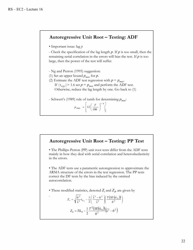
• Important issue: lag p

- Check the specification of the lag length p. If p is too small, then the remaining serial correlation in the errors will bias the test. If p is too large, then the power of the test will suffer.

- Ng and Perron (1995) suggestion: (1) Set an upper bound pmax for p. (2) Estimate the ADF test regression with p = pmax.

If |tα(p)|> 1.6 set p = pmax and perform the ADF test. Otherwise, reduce the lag length by one. Go back to (1)

- Schwert’s (1989) rule of tumb for determining pmax:


4/1

max 10012

Tp

• The Phillips-Perron (PP) unit root tests differ from the ADF tests mainly in how they deal with serial correlation and heteroskedasticity in the errors.

• The ADF tests use a parametric autoregression to approximate the ARMA structure of the errors in the test regression. The PP tests correct the DF tests by the bias induced by the omitted autocorrelation.

• These modified statistics, denoted Zt and Z, are given by.

Autoregressive Unit Root – Testing: PP Test

2

02

22

ˆ2

2

ˆ

ˆˆ

ˆˆ

2

1ˆˆ

0

SETtZ t

222

02

0 ˆˆˆ

ˆ

2

1ˆ

SETTZ


23

• The terms and are consistent estimates of the variance parameters:

• Under H0: α0 = 0, the PP Zt and Zα0 statistics have the same asymptotic distributions as the DF t-statistic and normalized bias statistics.

• PP tests tend to be more powerful than the ADF tests. But, they can severe size distortions (when autocorrelations of εt are negative) and they are more sensitive to model misspecification (order of ARMA model).


2

T

tt

TET

1

212 lim

T

t

T

tt

T TE

1 1

22 1lim

• Advantage of the PP tests over the ADF tests:

- Robust to general forms of heteroskedasticity in the error term εt.

- No need to specify a lag length for the ADF test regression.



24

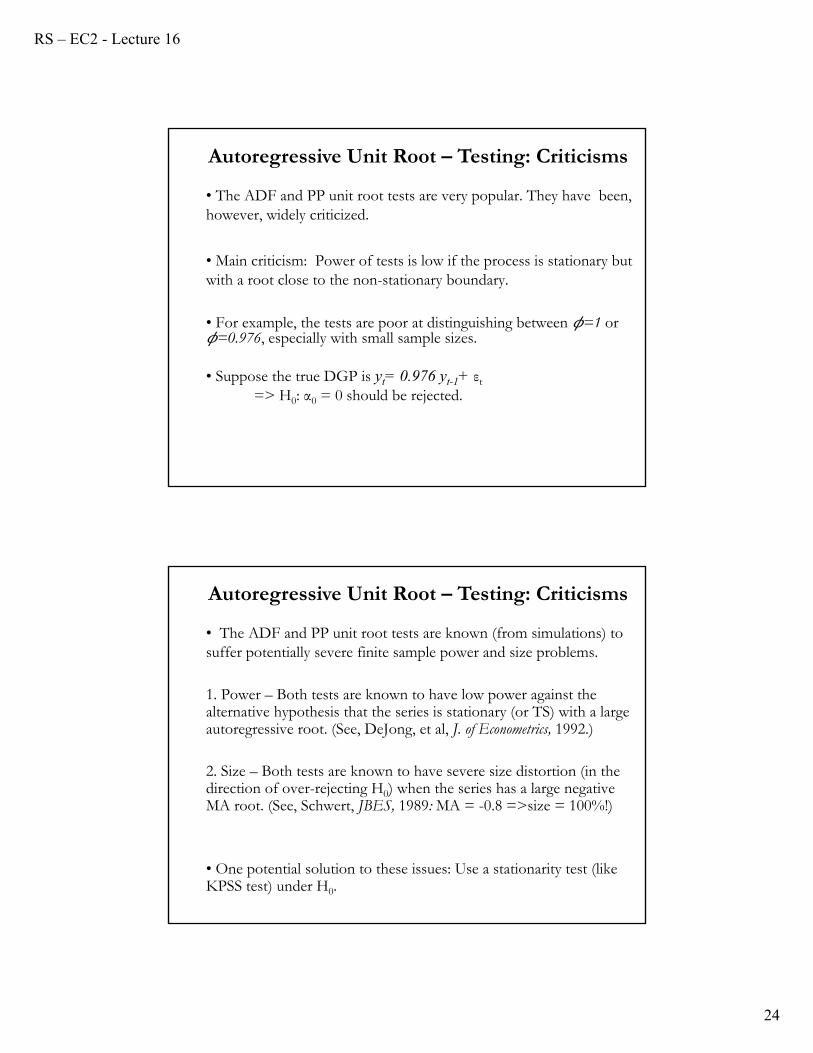
• The ADF and PP unit root tests are very popular. They have been, however, widely criticized.

• Main criticism: Power of tests is low if the process is stationary but with a root close to the non-stationary boundary.

• For example, the tests are poor at distinguishing between =1 or =0.976, especially with small sample sizes.

• Suppose the true DGP is yt= 0.976 yt-1+ εt

=> H0: α0 = 0 should be rejected.

Autoregressive Unit Root – Testing: Criticisms

• The ADF and PP unit root tests are known (from simulations) to suffer potentially severe finite sample power and size problems.

1. Power – Both tests are known to have low power against the alternative hypothesis that the series is stationary (or TS) with a large autoregressive root. (See, DeJong, et al, J. of Econometrics, 1992.)

2. Size – Both tests are known to have severe size distortion (in the direction of over-rejecting H0) when the series has a large negative MA root. (See, Schwert, JBES, 1989: MA = -0.8 =>size = 100%!)

• One potential solution to these issues: Use a stationarity test (like KPSS test) under H0.

Autoregressive Unit Root – Testing: Criticisms


25

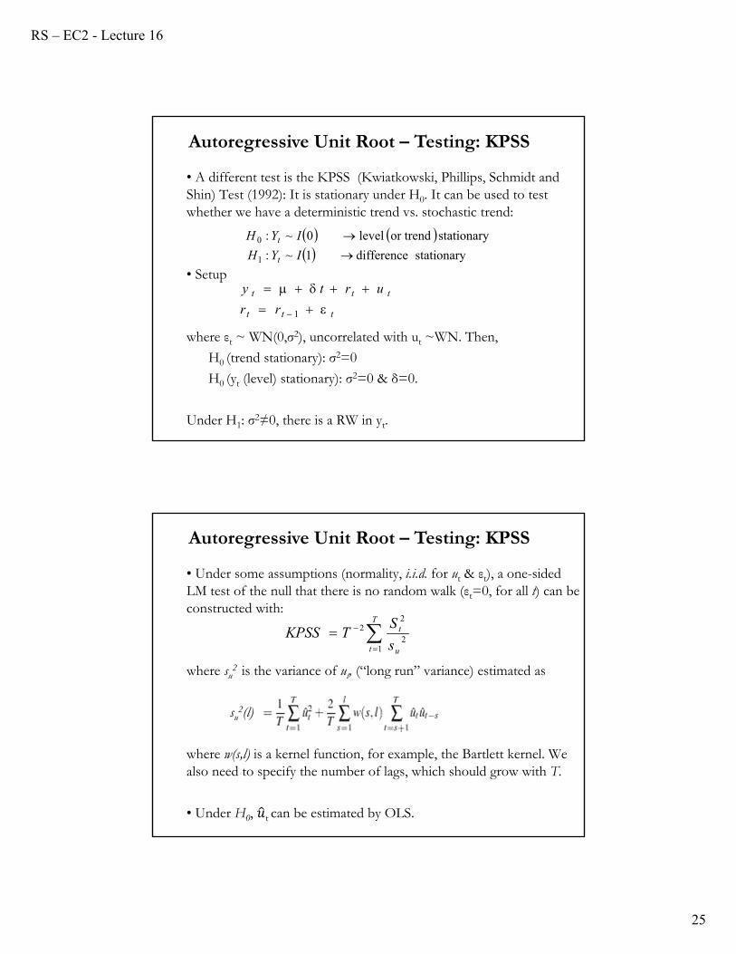
• A different test is the KPSS (Kwiatkowski, Phillips, Schmidt and Shin) Test (1992): It is stationary under H0. It can be used to test whether we have a deterministic trend vs. stochastic trend:

• Setup

where εt ~ WN(0,σ2), uncorrelated with ut ~WN. Then,

H0 (trend stationary): σ2=0

H0 (yt (level) stationary): σ2=0 & δ=0.

Under H1: σ2≠0, there is a RW in yt.

Autoregressive Unit Root – Testing: KPSS

stationary difference 1~:

stationary or trend level0~:

1

0

IYH

IYH

t

t

ttt

ttt

rr

urty

1

• Under some assumptions (normality, i.i.d. for ut & εt), a one-sided LM test of the null that there is no random walk (εt=0, for all t) can be constructed with:

where su2 is the variance of ut, (“long run” variance) estimated as

su2(l)

where w(s,l) is a kernel function, for example, the Bartlett kernel. We also need to specify the number of lags, which should grow with T.

• Under H0, t can be estimated by OLS.


T

t u

t

s

STKPSS

12

22


26

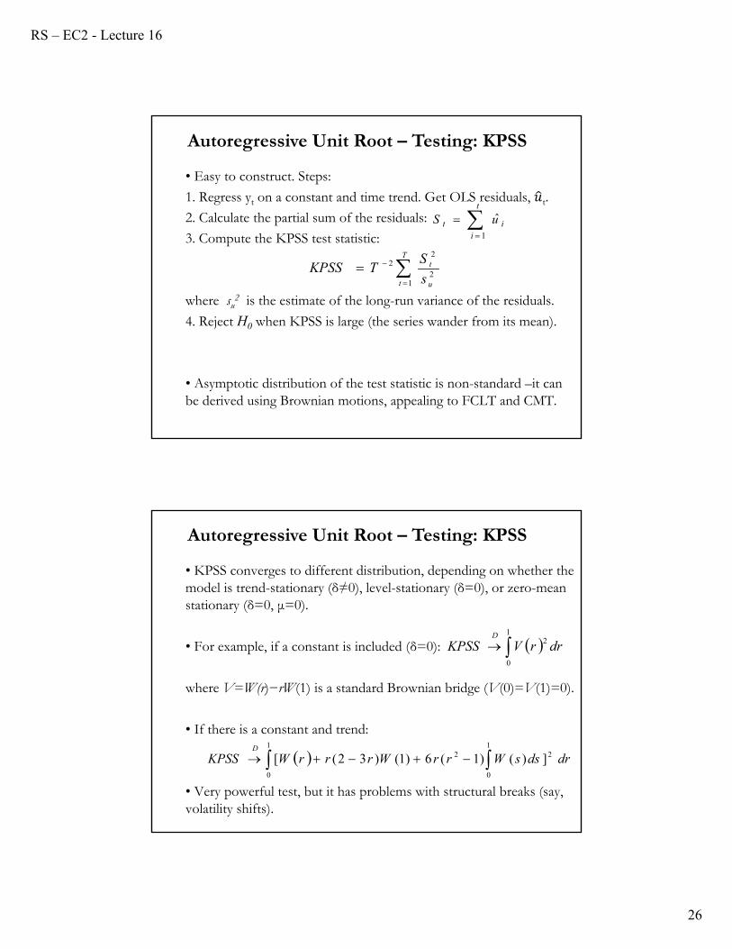
• Easy to construct. Steps:

1. Regress yt on a constant and time trend. Get OLS residuals, t.

2. Calculate the partial sum of the residuals:

3. Compute the KPSS test statistic:

where su2 is the estimate of the long-run variance of the residuals.

4. Reject H0 when KPSS is large (the series wander from its mean).

• Asymptotic distribution of the test statistic is non-standard –it can be derived using Brownian motions, appealing to FCLT and CMT.


t

iit uS

1

ˆ

T

t u

t

s

STKPSS

12

22

• KPSS converges to different distribution, depending on whether the model is trend-stationary (δ≠0), level-stationary (δ=0), or zero-mean stationary (δ=0, μ=0).

• For example, if a constant is included (δ=0):

where V=W(r)−rW(1) is a standard Brownian bridge (V(0)=V(1)=0).

• If there is a constant and trend:

• Very powerful test, but it has problems with structural breaks (say, volatility shifts).


1

0

2 drrVKPSSD

1

0

1

0

22 ])()1(6)1()32([ drdssWrrWrrrWKPSSD


27

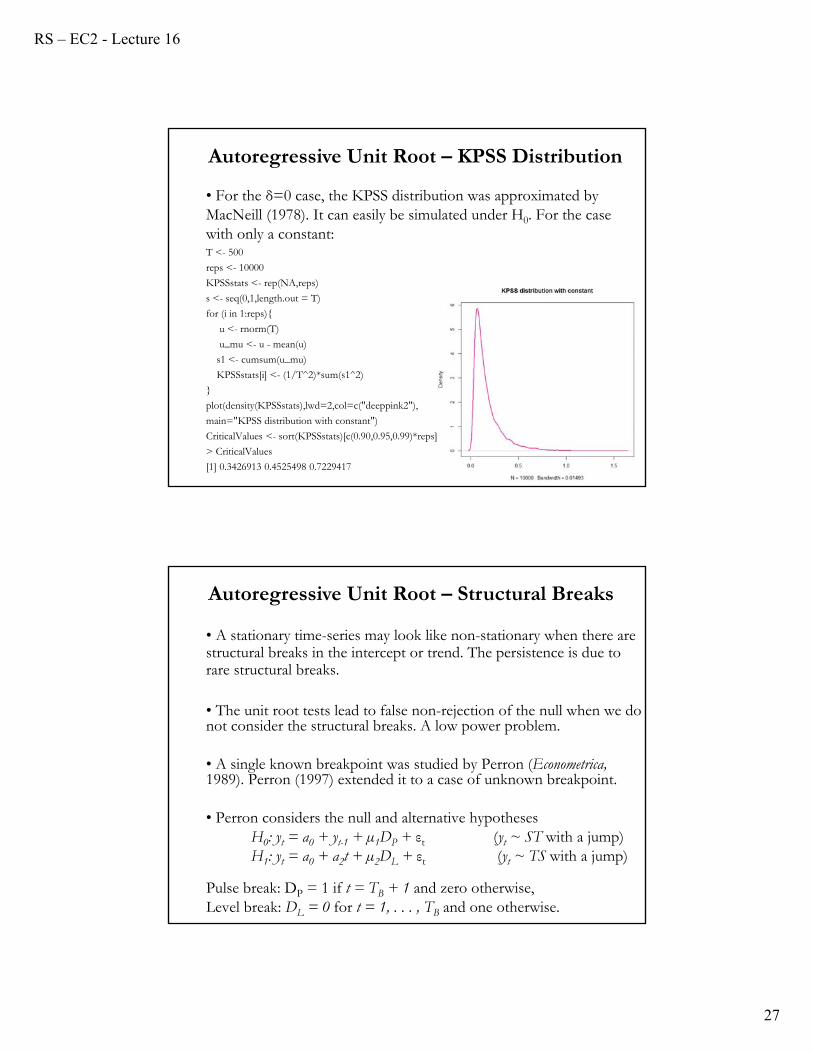
• For the δ=0 case, the KPSS distribution was approximated by MacNeill (1978). It can easily be simulated under H0. For the case with only a constant:T <- 500

reps <- 10000

KPSSstats <- rep(NA,reps)

s <- seq(0,1,length.out = T)

for (i in 1:reps){

u <- rnorm(T)

u_mu <- u - mean(u)

s1 <- cumsum(u_mu)

KPSSstats[i] <- (1/T^2)*sum(s1^2)

}

plot(density(KPSSstats),lwd=2,col=c("deeppink2"),

main="KPSS distribution with constant")

CriticalValues <- sort(KPSSstats)[c(0.90,0.95,0.99)*reps]

> CriticalValues

[1] 0.3426913 0.4525498 0.7229417

Autoregressive Unit Root – KPSS Distribution

• A stationary time-series may look like non-stationary when there are structural breaks in the intercept or trend. The persistence is due to rare structural breaks.

• The unit root tests lead to false non-rejection of the null when we do not consider the structural breaks. A low power problem.

• A single known breakpoint was studied by Perron (Econometrica, 1989). Perron (1997) extended it to a case of unknown breakpoint.

• Perron considers the null and alternative hypothesesH0: yt = a0 + yt-1 + µ1DP + εt (yt ~ ST with a jump)H1: yt = a0 + a2t + µ2DL + εt (yt ~ TS with a jump)

Pulse break: DP = 1 if t = TB + 1 and zero otherwise,Level break: DL = 0 for t = 1, . . . , TB and one otherwise.

Autoregressive Unit Root – Structural Breaks


28

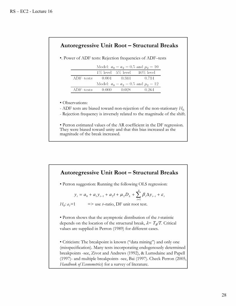
•. Power of ADF tests: Rejection frequencies of ADF–tests

• Observations:- ADF tests are biased toward non-rejection of the non-stationary H0.

- Rejection frequency is inversely related to the magnitude of the shift.

• Perron estimated values of the AR coefficient in the DF regression. They were biased toward unity and that this bias increased as the magnitude of the break increased.


• Perron suggestion: Running the following OLS regression:

H0: a1=1 => use t–ratio, DF unit root test.

• Perron shows that the asymptotic distribution of the t-statistic depends on the location of the structural break, = TB/T. Critical values are supplied in Perron (1989) for different cases.

• Criticism: The breakpoint is known (“data mining”) and only one (misspecification). Many tests incorporating endogenously determined breakpoints -see, Zivot and Andrews (1992), & Lumsdaine and Papell (1997)- and multiple breakpoints -see, Bai (1997). Check Perron (2005, Handbook of Econometrics) for a survey of literature.


0 1 1 2 21

p

t t L i t i ti

y a a y a t D y


29

• We can always decompose a unit root process into the sum of a random walk and a stable process. This is known as the Beveridge-Nelson (1981) (BN) composition.

• Let yt ~ I(1), rt ~ RW and ct ~I(0).yt = rt + ct.

Since ct is stable it has a Wold decomposition:

Then,

where ψ(1)=0. Then,

Autoregressive Unit Root - Relevance

)()1( tt LyL

tt

tttt

L

LLyL

*)()1(

))1()(()1( )()1(

ttttt crLLLy 11 )1(*)()1)(1(

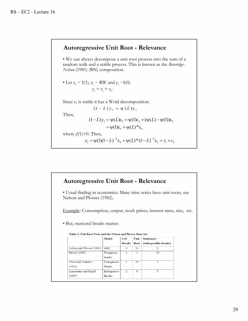
• Usual finding in economics: Many time series have unit roots, see Nelson and Plosser (1982).

Example: Consumption, output, stock prices, interest rates, size, etc.

• But, sturcural breaks matter.



30

• Usual finding in economics: Many time series have unit roots, see Nelson and Plosser (1982).

Example: Consumption, output, stock prices, interest rates, unemployment, size, compensation are usually I(1).

• Sometimes a linear combination of I(1) series produces an I(0). For example, (log consumption– log output) is stationary. This situation iscalled cointegration.

• Practical problems with cointegration:- Asymptotics change completely.- Not enough data to definitively say we have cointegration.


Documents

Lecture 16 Unit Root Tests - Bauer College of Business · RS – EC2 - Lecture 16 4 • Note that an OLS estimation of , under a unit root, involves taking averages of the integrated