17-1

Lecture 17

Outliers & Influential Observations

STAT 512

Spring 2011

Background Reading

KNNL: Sections 10.2-10.4

17-2

Topic Overview

• Statistical Methods for Identifying Outliers /

Influential Observations

• CDI/Physicians Case Study

• Remedial Measures

17-3

Outlier Detection in MLR

• We can have both X and Y outliers

• In SLR, outliers were relatively easy to detect

via scatterplots or residual plots.

• In MLR, it becomes more difficult to detect

outlier via simple plots.

o Univariate outliers may not be as extreme

in a MLR

o Some multivariate outliers may not be

detectable in single-variable analyses

17-4

Using Residuals Detecting Outliers in the Response (Y)

• Have seen how we can use residuals for

identifying problems with normality,

constancy of variance, linearity.

• Could also use residuals to identify outlying

values in Y (large magnitude implies

extreme value)

• Residuals don’t really have a “scale”, so....

What defines a large magnitude? Need

something more standard

17-5

Semi-studentized Residuals

• Recall that 2(0, )

iid

i Nε σ∼ , so: 0

(0,1)i Nε

σ

−∼ are “standardized errors”

• However, we don’t know the true errors or σ , so we use residuals and MSE .

• When you divide the residuals by MSE ,

you have semi-studentized residuals.

• Slightly better than regular residuals, can

use them in the same ways we used

residuals.

17-6

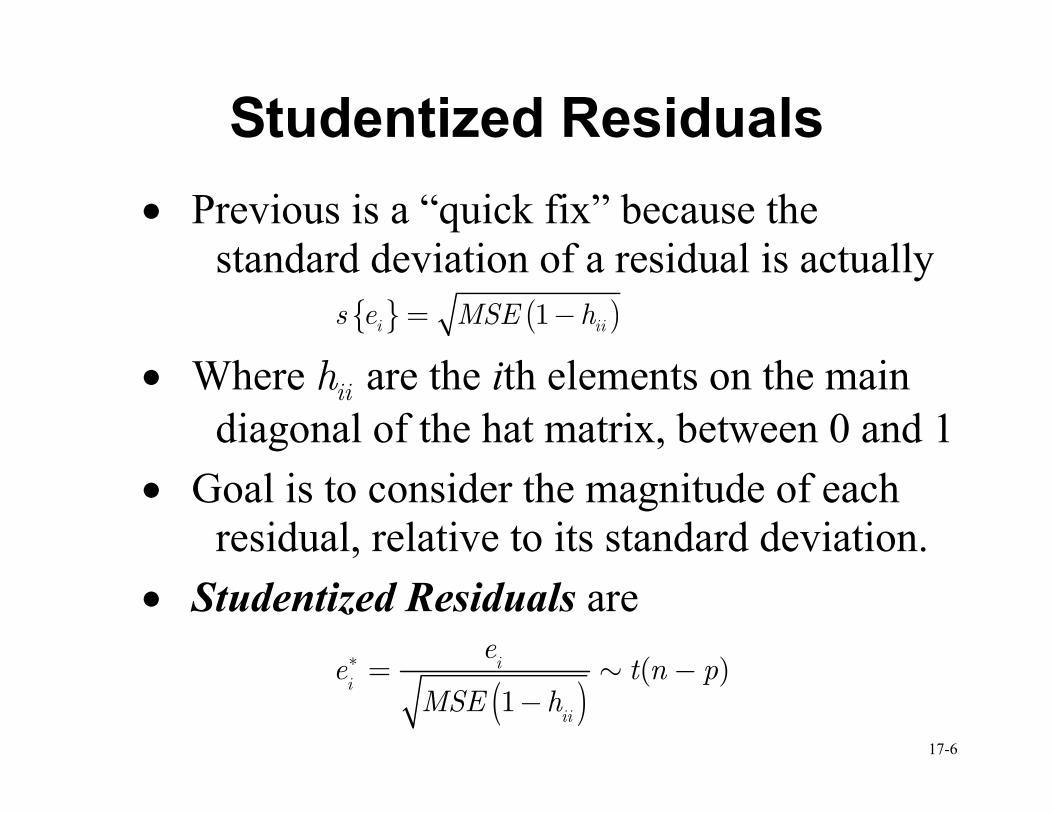
Studentized Residuals

• Previous is a “quick fix” because the

standard deviation of a residual is actually { } ( )1i iis e MSE h= −

• Where iih are the ith elements on the main

diagonal of the hat matrix, between 0 and 1

• Goal is to consider the magnitude of each

residual, relative to its standard deviation.

• Studentized Residuals are

( )( )

1

i

i

ii

ee t n p

MSE h

∗ = −−

∼

17-7

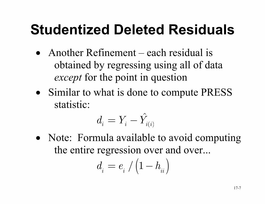
Studentized Deleted Residuals

• Another Refinement – each residual is

obtained by regressing using all of data

except for the point in question

• Similar to what is done to compute PRESS

statistic:

( )ˆ

i i i id Y Y= −

• Note: Formula available to avoid computing

the entire regression over and over...

( )/ 1i i iid e h= −

17-8

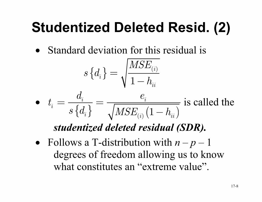
Studentized Deleted Resid. (2)

• Standard deviation for this residual is

{ } ( )

1

i

i

ii

MSEs d

h=

−

•

{ }( ) ( )1

i ii

i i ii

d ets d MSE h

= =−

is called the

studentized deleted residual (SDR).

• Follows a T-distribution with n – p – 1

degrees of freedom allowing us to know

what constitutes an “extreme value”.

17-9

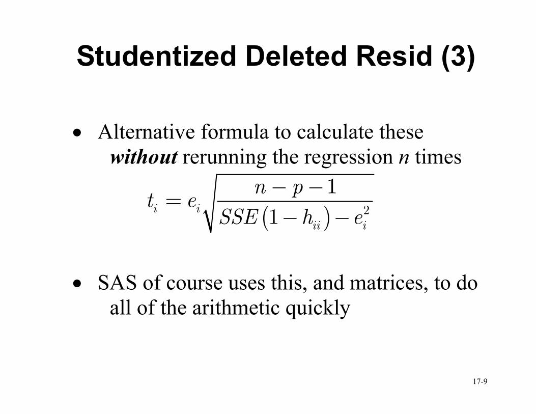
Studentized Deleted Resid (3)

• Alternative formula to calculate these

without rerunning the regression n times

( ) 2

1

1i i

ii i

n pt e

SSE h e

− −=

− −

• SAS of course uses this, and matrices, to do

all of the arithmetic quickly

17-10

Using Studentized Residuals

• Both studentized and studentized deleted

residuals can be quite useful for identifying

outliers

• Since we know they have a T-distribution,

for reasonable size n, an SDR of

magnitude 3 or more (in abs. value) will be

considered an outlier. Any with magnitude

between 2-3 may be close depending on

significance level used (see tables).

• Many high SDR indicates inadequate model.

17-11

Regular vs. “Deleted”

• Both generally tend to give similar

information.

• “Deleted” perhaps is the preferred method

since this method means that each data

point is not used in computing its own

residual and gives us something to

compare to as an “extreme value”.

17-12

Formal Test for Outliers in Y

• Test each of the n residuals to determine if it

is an outlier.

• Bonferroni used to adjust for the n tests –

significance level becomes 0.05 / n.

• Compare studentized deleted residuals (in

absolute value) to a T-critical value using

the above alpha, and n – p – 1 degrees of

freedom

• SDR’s that are larger in magnitude than the

critical value identify outliers.

17-13

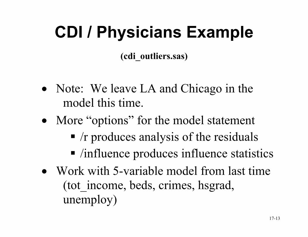
CDI / Physicians Example

(cdi_outliers.sas)

• Note: We leave LA and Chicago in the

model this time.

• More “options” for the model statement

� /r produces analysis of the residuals

� /influence produces influence statistics

• Work with 5-variable model from last time

(tot_income, beds, crimes, hsgrad,

unemploy)

17-14

Example (2)

proc reg data=cdi outest=fits; model lphys = beds tot_income hsgrad crimes unemploy /r; run;

• Produces several pages of output since each

residual information is given for each of

the 440 data points

• We’ll look at only a small part of this

output, for illustration

17-15

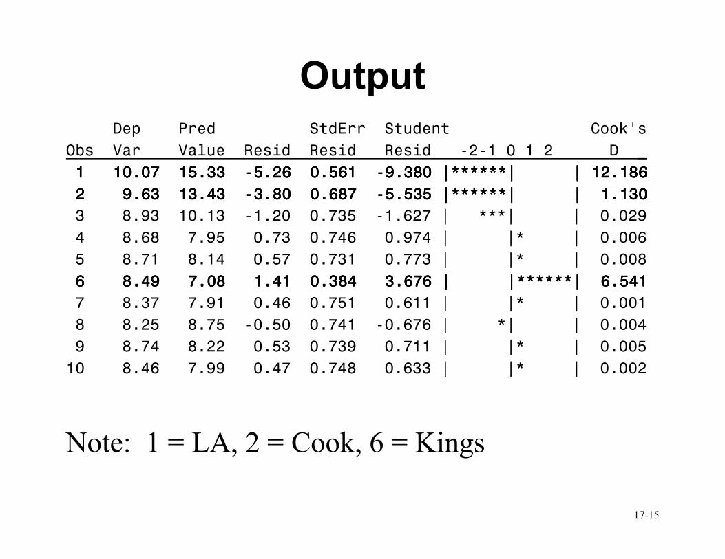
Output Dep Pred StdErr Student Cook's

Obs Var Value Resid Resid Resid -2-1 0 1 2 D _

1 10.07 15.33 1 10.07 15.33 1 10.07 15.33 1 10.07 15.33 ----5.26 0.561 5.26 0.561 5.26 0.561 5.26 0.561 ----9.380 |******| | 12.1869.380 |******| | 12.1869.380 |******| | 12.1869.380 |******| | 12.186

2 9.63 13.43 2 9.63 13.43 2 9.63 13.43 2 9.63 13.43 ----3.80 0.687 3.80 0.687 3.80 0.687 3.80 0.687 ----5.535 |******| | 1.1305.535 |******| | 1.1305.535 |******| | 1.1305.535 |******| | 1.130

3 8.93 10.13 -1.20 0.735 -1.627 | ***| | 0.029

4 8.68 7.95 0.73 0.746 0.974 | |* | 0.006

5 8.71 8.14 0.57 0.731 0.773 | |* | 0.008

6 8.49 7.08 1.41 0.384 3.676 | |******| 6.5416 8.49 7.08 1.41 0.384 3.676 | |******| 6.5416 8.49 7.08 1.41 0.384 3.676 | |******| 6.5416 8.49 7.08 1.41 0.384 3.676 | |******| 6.541

7 8.37 7.91 0.46 0.751 0.611 | |* | 0.001

8 8.25 8.75 -0.50 0.741 -0.676 | *| | 0.004

9 8.74 8.22 0.53 0.739 0.711 | |* | 0.005

10 8.46 7.99 0.47 0.748 0.633 | |* | 0.002

Note: 1 = LA, 2 = Cook, 6 = Kings

17-16

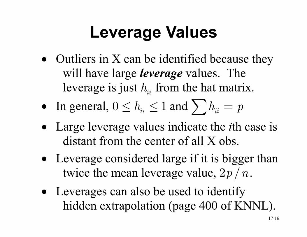
Leverage Values

• Outliers in X can be identified because they

will have large leverage values. The

leverage is just iih from the hat matrix.

• In general, 0 1iih≤ ≤ and iih p=∑

• Large leverage values indicate the ith case is

distant from the center of all X obs.

• Leverage considered large if it is bigger than

twice the mean leverage value, 2 /p n .

• Leverages can also be used to identify

hidden extrapolation (page 400 of KNNL).

17-17

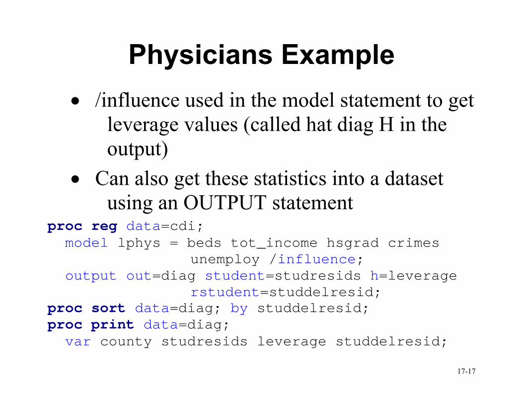
Physicians Example

• /influence used in the model statement to get

leverage values (called hat diag H in the

output)

• Can also get these statistics into a dataset

using an OUTPUT statement proc reg data=cdi; model lphys = beds tot_income hsgrad crimes unemploy /influence; output out=diag student=studresids h=leverage rstudent=studdelresid; proc sort data=diag; by studdelresid; proc print data=diag; var county studresids leverage studdelresid;

17-18

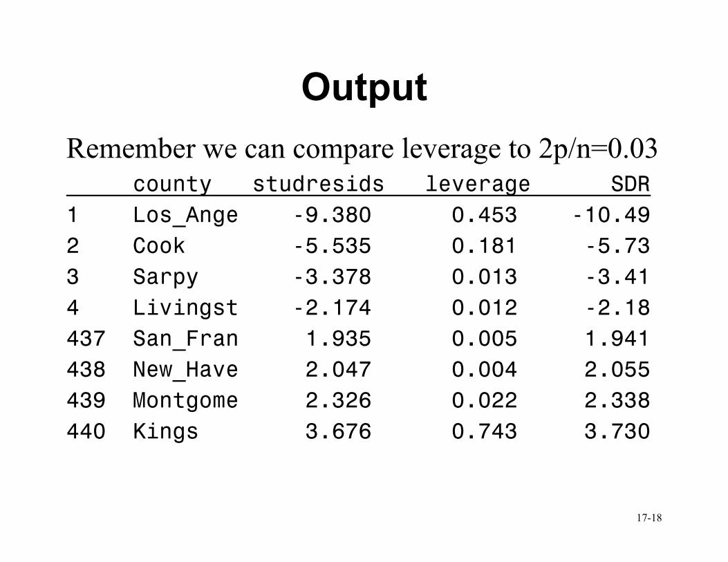
Output

Remember we can compare leverage to 2p/n=0.03 county studresids leverage SDR

1 Los_Ange -9.380 0.453 -10.49

2 Cook -5.535 0.181 -5.73

3 Sarpy -3.378 0.013 -3.41

4 Livingst -2.174 0.012 -2.18

437 San_Fran 1.935 0.005 1.941

438 New_Have 2.047 0.004 2.055

439 Montgome 2.326 0.022 2.338

440 Kings 3.676 0.743 3.730

17-19

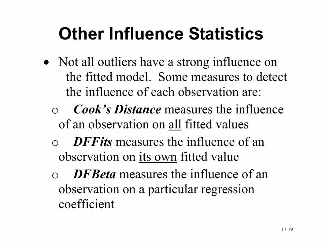
Other Influence Statistics

• Not all outliers have a strong influence on

the fitted model. Some measures to detect

the influence of each observation are:

o Cook’s Distance measures the influence of an observation on all fitted values

o DFFits measures the influence of an observation on its own fitted value

o DFBeta measures the influence of an observation on a particular regression

coefficient

17-20

Cook’s Distance

• Assess the influence of a data point in ALL

predicted values

• Obtain from SAS using /r

• Large values suggest that an observation has

a lot of influence (can compare to an

F(p, n-p) distribution).

17-21

DFFits

• Assess the influence of a data point in ITS

OWN prediction only

• Obtain from SAS using /influence

• Essentially measures difference between

prediction of itself with/without using that

observation in the computation

• Large absolute values (bigger than 1, or

bigger than 2 /p n ) suggest that an

observation has a lot of influence on its

own prediction

17-22

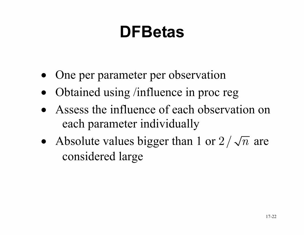
DFBetas

• One per parameter per observation

• Obtained using /influence in proc reg

• Assess the influence of each observation on

each parameter individually

• Absolute values bigger than 1 or 2/ n are considered large

17-23

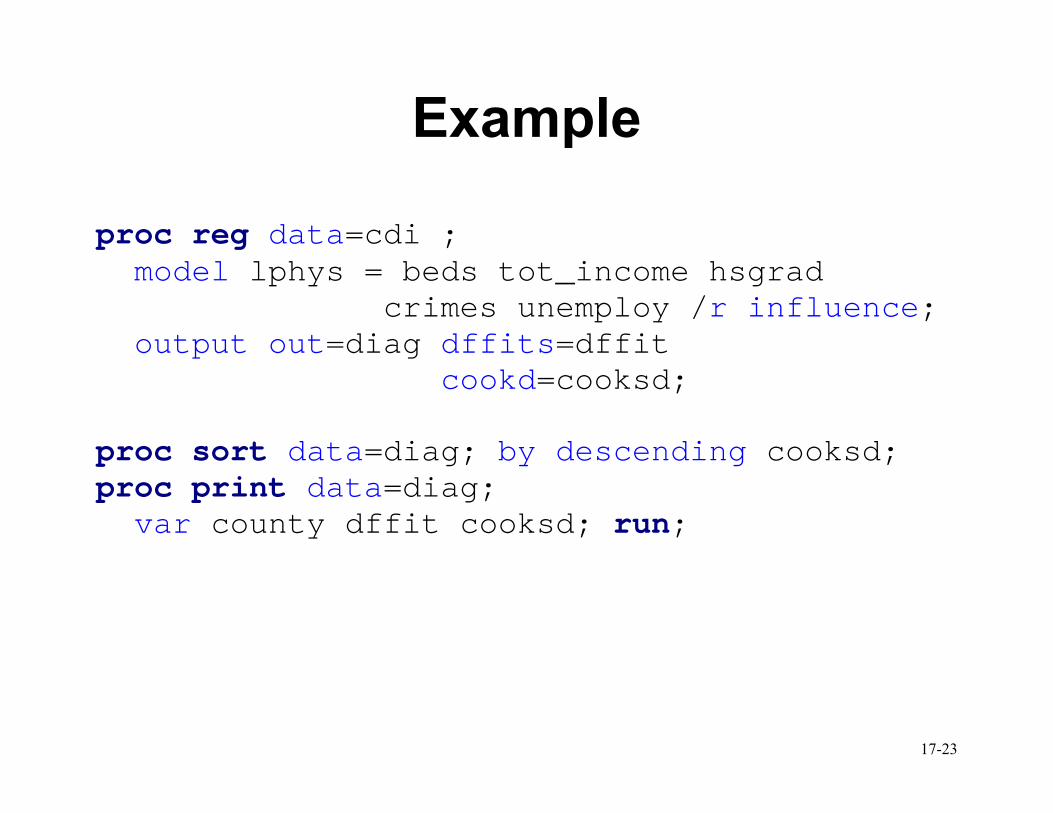
Example

proc reg data=cdi ; model lphys = beds tot_income hsgrad crimes unemploy /r influence; output out=diag dffits=dffit cookd=cooksd; proc sort data=diag; by descending cooksd; proc print data=diag; var county dffit cooksd; run;

17-24

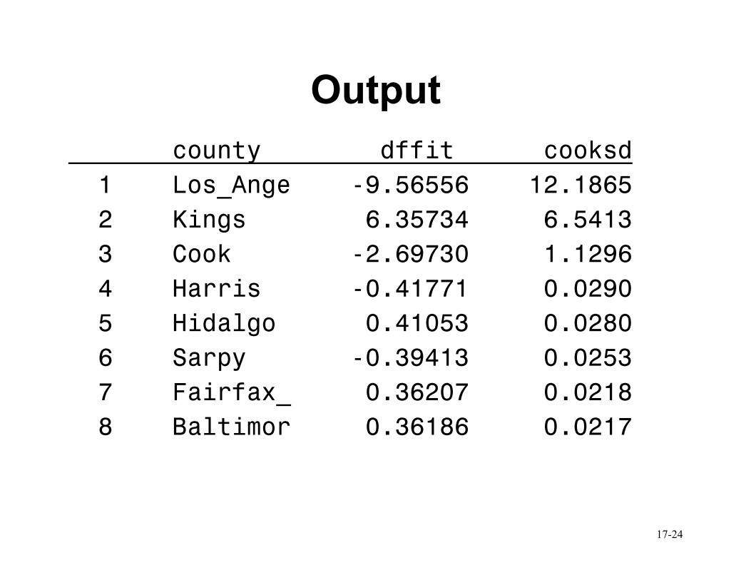
Output

county dffit cooksd

1 Los_Ange -9.56556 12.1865

2 Kings 6.35734 6.5413

3 Cook -2.69730 1.1296

4 Harris -0.41771 0.0290

5 Hidalgo 0.41053 0.0280

6 Sarpy -0.39413 0.0253

7 Fairfax_ 0.36207 0.0218

8 Baltimor 0.36186 0.0217

17-25

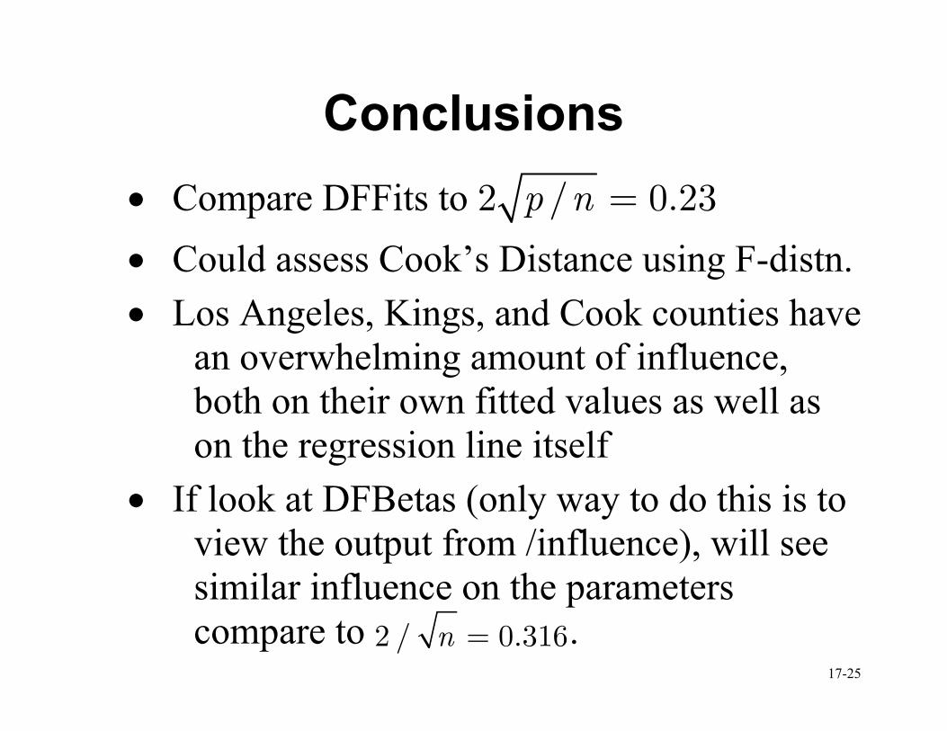
Conclusions

• Compare DFFits to 2 / 0.23p n =

• Could assess Cook’s Distance using F-distn.

• Los Angeles, Kings, and Cook counties have

an overwhelming amount of influence,

both on their own fitted values as well as

on the regression line itself

• If look at DFBetas (only way to do this is to

view the output from /influence), will see

similar influence on the parameters

compare to 2 / 0.316n = .

17-26

Influential Observations

• Big question now is, once we identify an

outlier, or influential observation, what do

we do with it?

• For a good understanding of the regression

model, the analysis IS needed. In our

example, we now know that we have three

cases holding a lot of influence. We may

want to....

� See what happens when we exclude these from the

model.

� Investigate these cases separately.

17-27

What not to do...

• Never simply exclude / ignore a data point

just because you don’t like what it does to

the results

• Never ignore the fact that you have one or

two overly influential observations

17-28

Some Remedial Measures

• See Section 11.3

• Robust Regression procedures decrease the

emphasis of outlying observations

• Doing this is slightly beyond the scope of

the class, but it doesn’t hurt to be aware

that such methods exist.

17-29

Upcoming in Lecture 18...

• Miscellaneous topics in MLR.

o Chapter 8, Section 10.1