1

Lecture 2: Data Management

Ing-Ray Chen

CS 6204 Mobile Computing

Virginia Tech

Courtesy of G.G. Richard III for providing some of

the slides

2

Communications Asymmetry in

Mobile Wireless Environments

• Network asymmetry

– In many cases, downlink bandwidth far exceeds

uplink bandwidth

• Client-to-server ratio

– Large client population, but few servers

• Data volume

– Small requests, large responses

– Downlink bandwidth more important

• Update-oriented communication

– Updates likely affect a number of clients

3

Disseminating Data to Wireless Hosts

• Broadcast-oriented dissemination makes sense for many applications

• Can be one-way or with feedback

– Sports

– Stock prices

– New software releases

– Chess matches

– Music

– Election Coverage

– Weather/traffic …

4

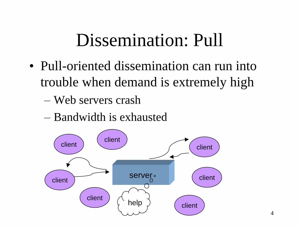
Dissemination: Pull

• Pull-oriented dissemination can run into

trouble when demand is extremely high

– Web servers crash

– Bandwidth is exhausted

client

client

client

client client

client

client

server

help

5

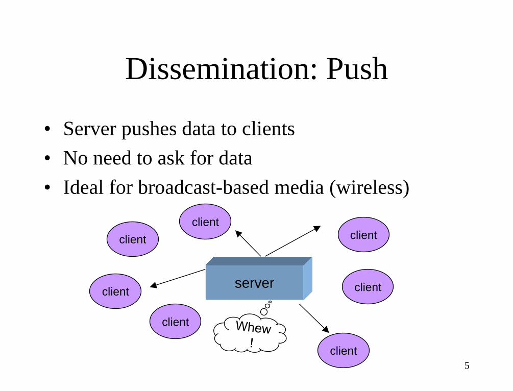
Dissemination: Push

• Server pushes data to clients

• No need to ask for data

• Ideal for broadcast-based media (wireless)

client

client

client

client client

client

client

server

6

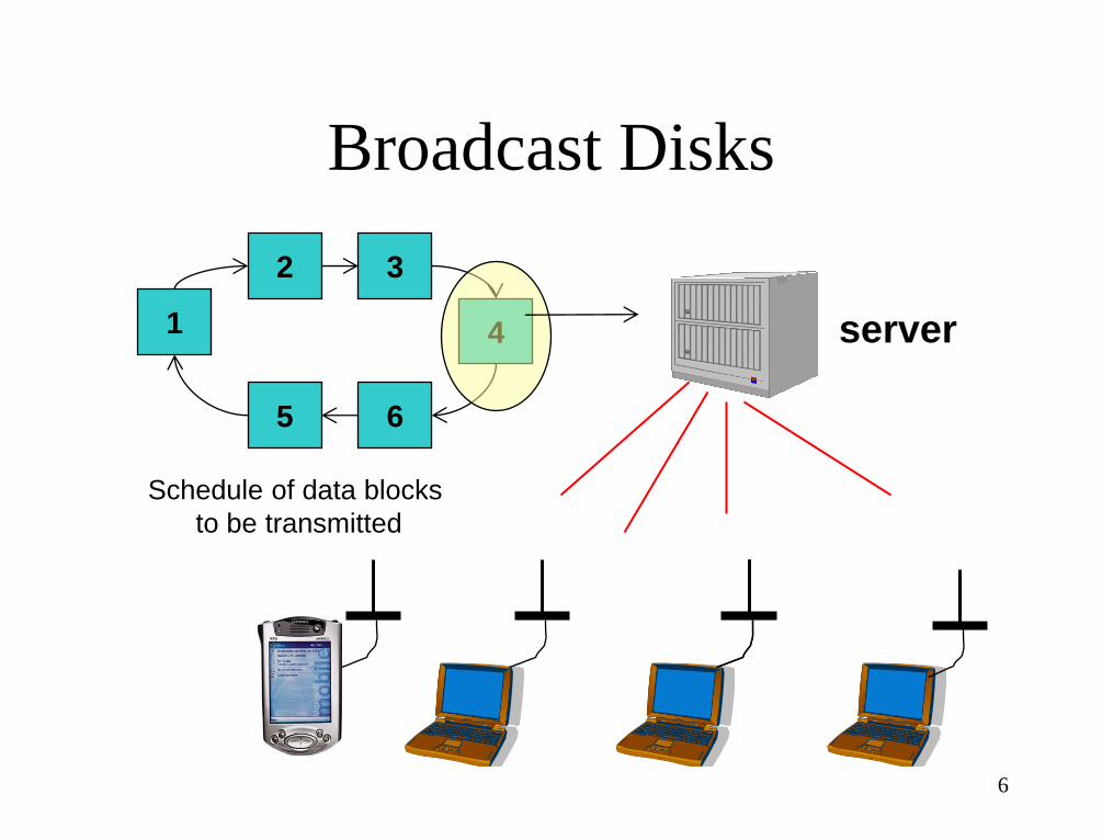
Broadcast Disks

1

2 3

4

5 6

server

Schedule of data blocks

to be transmitted

7

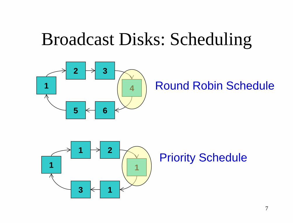
Broadcast Disks: Scheduling

1

2 3

4

5 6

Round Robin Schedule

1

1 2

1

3 1

Priority Schedule

8

Priority Scheduling (2)

• Random

– Randomize broadcast schedule

– Broadcast "hotter" items more frequently

• Periodic Broadcast Program

– Create a schedule that broadcasts hotter items

more frequently……but schedule is fixed

– Assumptions

• Data is read-only

• Schedule is computed and doesn't change…

• Access patterns of MUs are assumed the same

Allows mobile hosts to sleep…

9

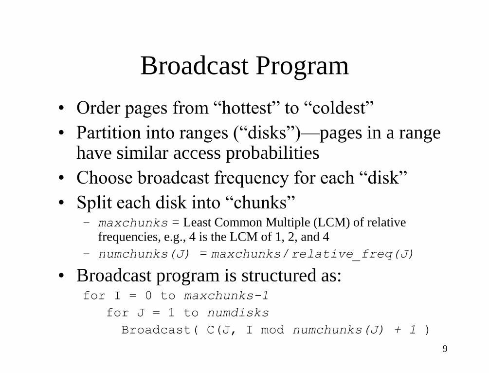
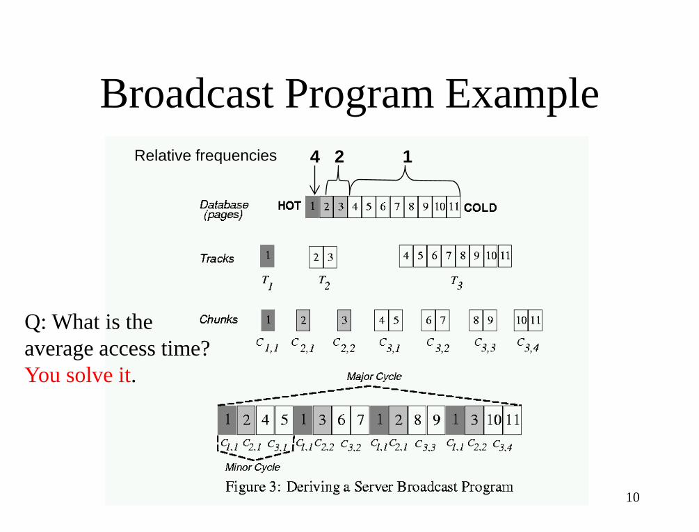
Broadcast Program

• Order pages from “hottest” to “coldest”

• Partition into ranges (“disks”)—pages in a range have similar access probabilities

• Choose broadcast frequency for each “disk”

• Split each disk into “chunks” – maxchunks = Least Common Multiple (LCM) of relative

frequencies, e.g., 4 is the LCM of 1, 2, and 4

– numchunks(J) = maxchunks / relative_freq(J)

• Broadcast program is structured as: for I = 0 to maxchunks-1

for J = 1 to numdisks

Broadcast( C(J, I mod numchunks(J) + 1 )

10

Broadcast Program Example

Relative frequencies 4 2 1

Q: What is the

average access time?

You solve it.

11

Air Indexing (Ref. [5])

• Air indexing

– Broadcast not only data, but also index

– Clients listen to the index to predict the arrival of desired data

– Clients sleep and wake up to receive data

• Performance Measures

– Access-time (response time)

• Time elapsed from issuing a query to receiving data

– Tuning-time (power-on time)

• Time elapsed by client staying active to retrieve data

12

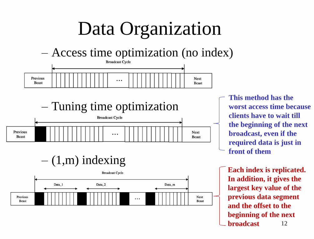
Data Organization

– Access time optimization (no index)

– Tuning time optimization

– (1,m) indexing

This method has the

worst access time because

clients have to wait till

the beginning of the next

broadcast, even if the

required data is just in

front of them

Each index is replicated.

In addition, it gives the

largest key value of the

previous data segment

and the offset to the

beginning of the next

broadcast

13

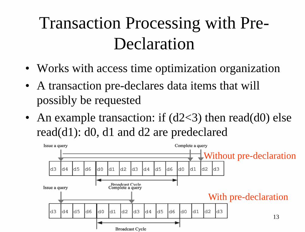
Transaction Processing with Pre-

Declaration

• Works with access time optimization organization

• A transaction pre-declares data items that will

possibly be requested

• An example transaction: if (d2<3) then read(d0) else

read(d1): d0, d1 and d2 are predeclared

With pre-declaration

Without pre-declaration

14

Transaction Processing with Pre-

Declaration and Selective Tuning

• Works with tuning time optimization and

(1,m) indexing organization

– Initial probe

• Locate the next nearest index

– Index search

• Search the index to locate the desired data

– Data retrieval

• Tune into the channel at the particular point to

download the data

15

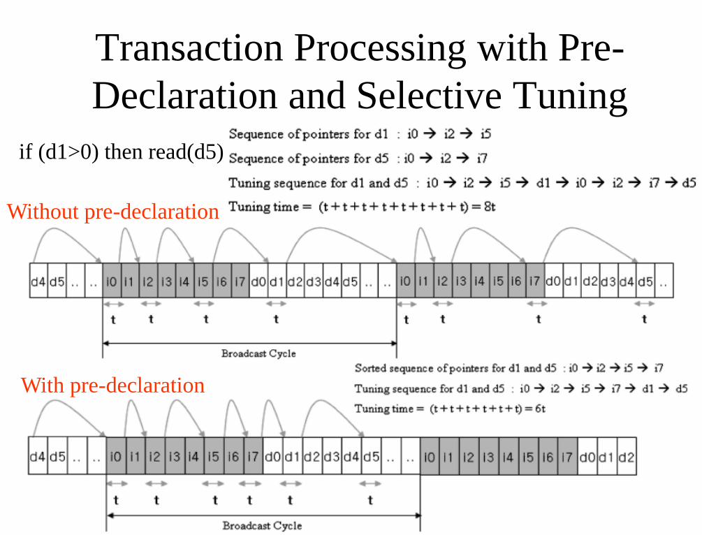
Transaction Processing with Pre-

Declaration and Selective Tuning

Without pre-declaration

With pre-declaration

if (d1>0) then read(d5)

16

Analysis of Pre-declaration with

Selective Tuning in Data Broadcast

–Access Time Optimization

• Access Time:

• Tuning Time

= Access Time

–Tuning Time Optimization

• Access Time:

• Tuning Time:

– (1, m) Indexing

• Access Time:

• Tuning Time: Same as that in the tuning time optimization organization

D # of items

I # of indices

op # of items in the transaction

n # of keys plus pointers one

tree node can hold

m # of times index is broadcast

k # of levels in the index tree

Number of revisits at level i

of the index tree

# of nodes at level i

Wait time for the

Broadcast cycle

Number of pages visited

to access an item (1 to go to begin

of index and 1 to retrieve the page)

Time to access op

data items

17

Hot For You Ain't Hot for Me

• Hottest data items are not necessarily the ones most frequently accessed by a particular client

• Access patterns may have changed

• Higher priority may be given to other clients

• Might be the only client that considers a particular data item important…

• Solution: caching

– needs to consider not only probability of access (standard caching), but also broadcast frequency

18

Broadcast Disks: Caching

• Under traditional caching schemes, usually want to cache "hottest" data

• What to cache with broadcast disks?

• Hottest?

– Probably not—that data will come around soon!

• Coldest?

– Ummmm…not necessarily…

19

Caching

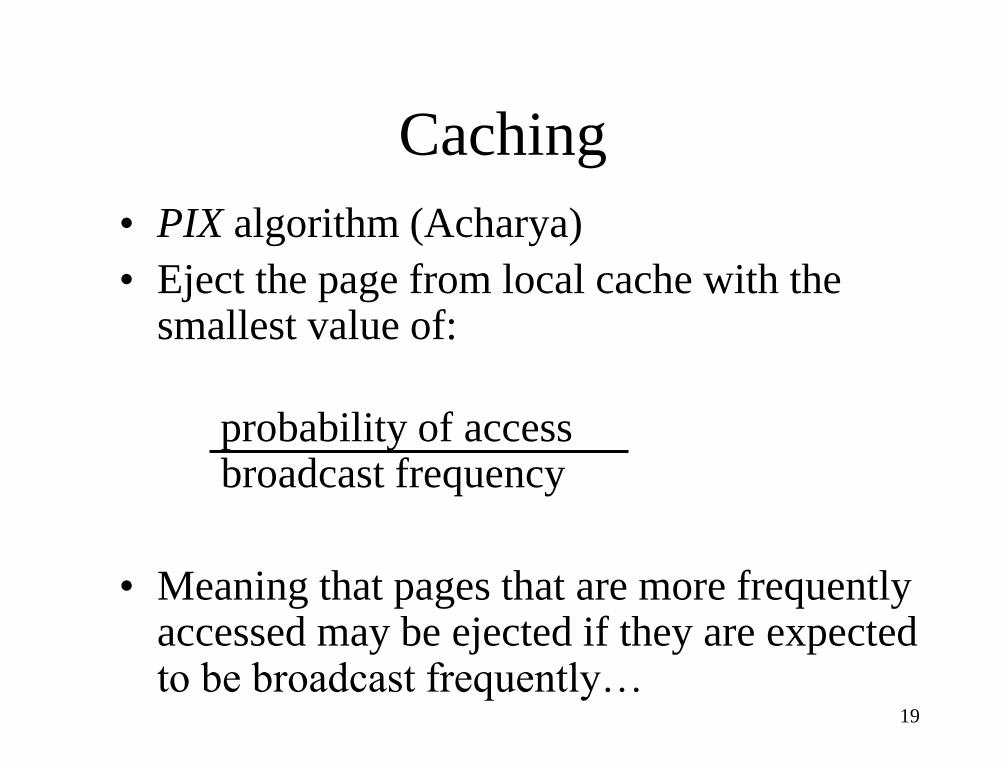
• PIX algorithm (Acharya)

• Eject the page from local cache with the smallest value of:

probability of access broadcast frequency

• Meaning that pages that are more frequently accessed may be ejected if they are expected to be broadcast frequently…

20

System Design: Hybrid Push/Pull?

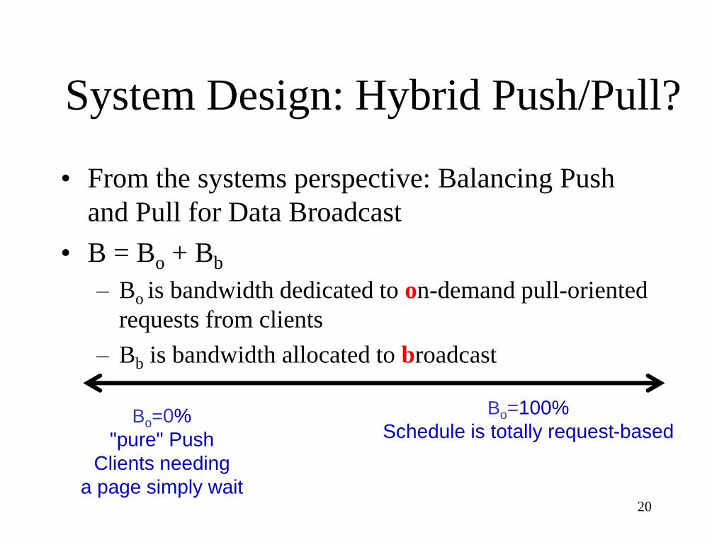
• From the systems perspective: Balancing Push

and Pull for Data Broadcast

• B = Bo + Bb

– Bo is bandwidth dedicated to on-demand pull-oriented

requests from clients

– Bb is bandwidth allocated to broadcast

Bo=0%

"pure" Push

Clients needing

a page simply wait

Bo=100%

Schedule is totally request-based

21

Optimal Bandwidth Allocation

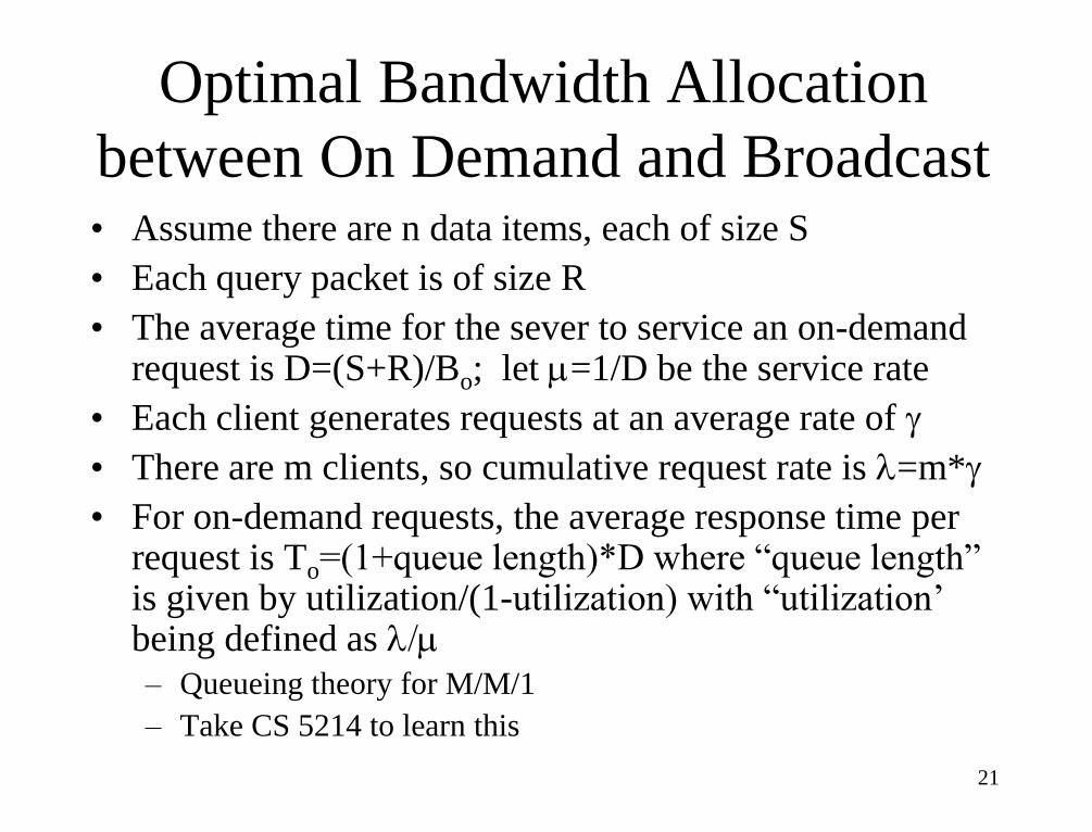
between On Demand and Broadcast • Assume there are n data items, each of size S

• Each query packet is of size R

• The average time for the sever to service an on-demand request is D=(S+R)/Bo; let m=1/D be the service rate

• Each client generates requests at an average rate of g

• There are m clients, so cumulative request rate is l=m*g

• For on-demand requests, the average response time per request is To=(1+queue length)*D where “queue length” is given by utilization/(1-utilization) with “utilization’ being defined as l/m

– Queueing theory for M/M/1

– Take CS 5214 to learn this

22

Optimal Bandwidth Allocation

between On Demand and Broadcast

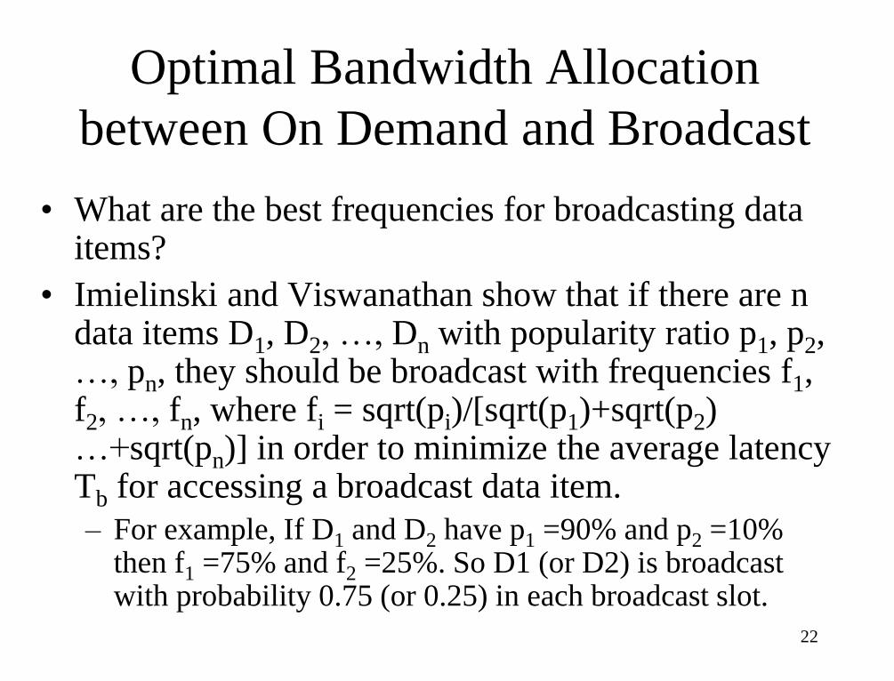
• What are the best frequencies for broadcasting data items?

• Imielinski and Viswanathan show that if there are n data items D1, D2, …, Dn with popularity ratio p1, p2, …, pn, they should be broadcast with frequencies f1, f2, …, fn, where fi = sqrt(pi)/[sqrt(p1)+sqrt(p2) …+sqrt(pn)] in order to minimize the average latency Tb for accessing a broadcast data item.

– For example, If D1 and D2 have p1 =90% and p2 =10% then f1 =75% and f2 =25%. So D1 (or D2) is broadcast with probability 0.75 (or 0.25) in each broadcast slot.

23

Optimal Bandwidth Allocation

between On Demand and Broadcast

• T=Tb + To is the average time to access a data item

• Imielinski and Viswanathan’s algorithm: Assign D1, D2, …, Di to broadcast channel

Assign Di+1, Di+2, …, Dn to on-demand channel

Determine optimal Bb, Bo to minimize T = Tb+ To:

Compute To by modeling on-demand channel as

M/M/1 (or M/D/1)

Compute Tb by using the optimal

frequencies f1, f2, …, fi

Compute optimal Bb which minimizes T to

within an acceptable threshold L

How? You solve it

24

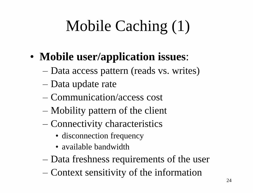
Mobile Caching (1)

• Mobile user/application issues:

– Data access pattern (reads vs. writes)

– Data update rate

– Communication/access cost

– Mobility pattern of the client

– Connectivity characteristics

• disconnection frequency

• available bandwidth

– Data freshness requirements of the user

– Context sensitivity of the information

25

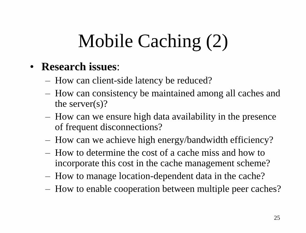
Mobile Caching (2)

• Research issues:

– How can client-side latency be reduced?

– How can consistency be maintained among all caches and the server(s)?

– How can we ensure high data availability in the presence of frequent disconnections?

– How can we achieve high energy/bandwidth efficiency?

– How to determine the cost of a cache miss and how to incorporate this cost in the cache management scheme?

– How to manage location-dependent data in the cache?

– How to enable cooperation between multiple peer caches?

26

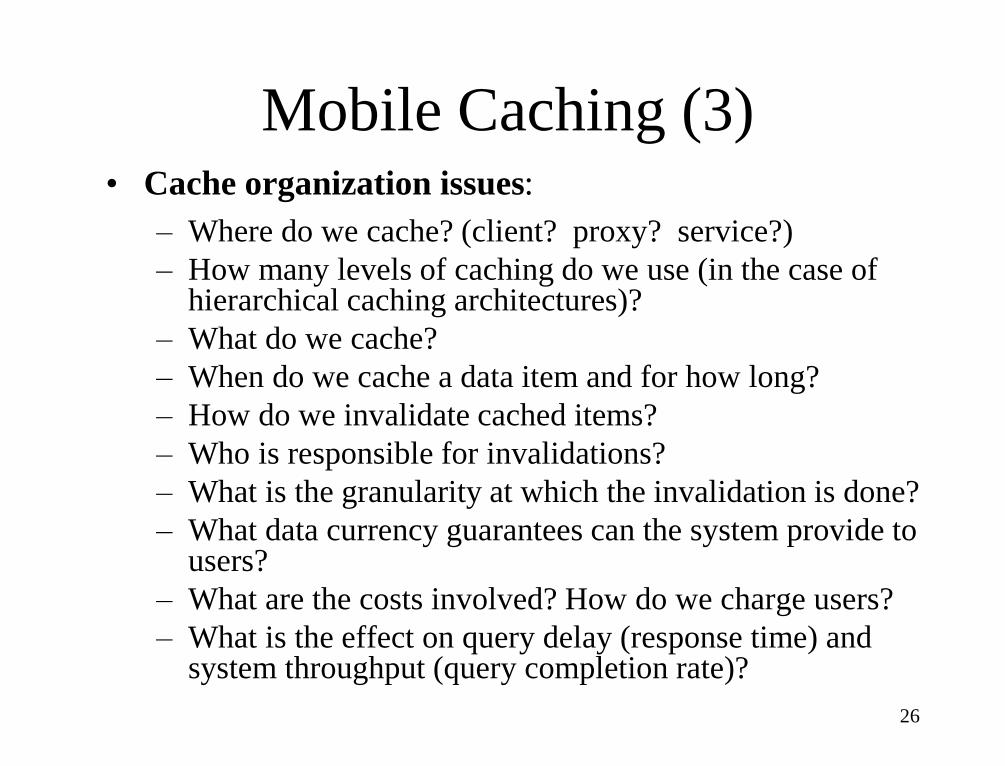
Mobile Caching (3) • Cache organization issues:

– Where do we cache? (client? proxy? service?)

– How many levels of caching do we use (in the case of hierarchical caching architectures)?

– What do we cache?

– When do we cache a data item and for how long?

– How do we invalidate cached items?

– Who is responsible for invalidations?

– What is the granularity at which the invalidation is done?

– What data currency guarantees can the system provide to users?

– What are the costs involved? How do we charge users?

– What is the effect on query delay (response time) and system throughput (query completion rate)?

27

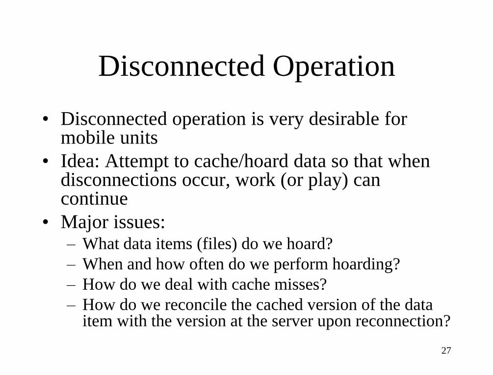
Disconnected Operation

• Disconnected operation is very desirable for mobile units

• Idea: Attempt to cache/hoard data so that when disconnections occur, work (or play) can continue

• Major issues: – What data items (files) do we hoard?

– When and how often do we perform hoarding?

– How do we deal with cache misses?

– How do we reconcile the cached version of the data item with the version at the server upon reconnection?

28

States of Operation

Data Hoarding

Disconnected

Read/write Reintegration

29

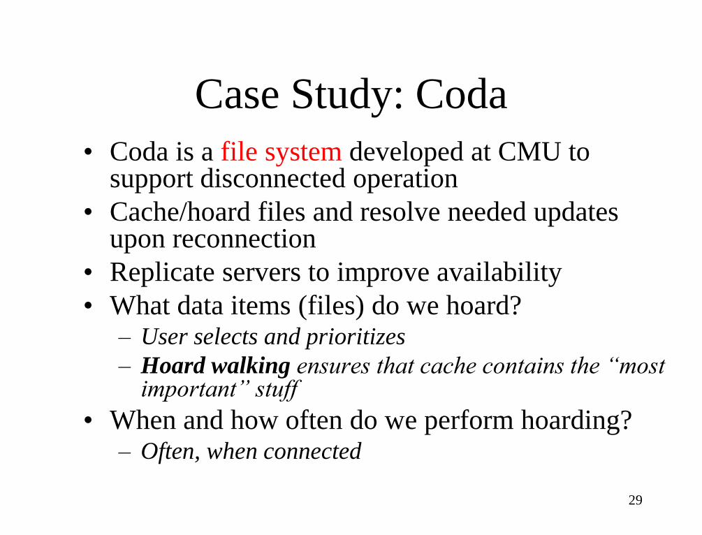
Case Study: Coda

• Coda is a file system developed at CMU to support disconnected operation

• Cache/hoard files and resolve needed updates upon reconnection

• Replicate servers to improve availability

• What data items (files) do we hoard? – User selects and prioritizes

– Hoard walking ensures that cache contains the “most important” stuff

• When and how often do we perform hoarding? – Often, when connected

30

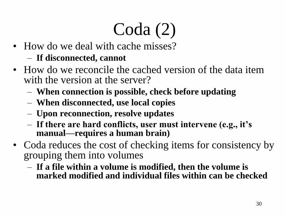
Coda (2) • How do we deal with cache misses?

– If disconnected, cannot

• How do we reconcile the cached version of the data item with the version at the server? – When connection is possible, check before updating

– When disconnected, use local copies

– Upon reconnection, resolve updates

– If there are hard conflicts, user must intervene (e.g., it’s manual—requires a human brain)

• Coda reduces the cost of checking items for consistency by grouping them into volumes – If a file within a volume is modified, then the volume is

marked modified and individual files within can be checked

31

To Cache or Not?

• Compare static allocation “always cache” (SA-always), “never cache” (SA-never), vs. dynamic allocation (DA)

• Cost model: – Each rm (read at mobile) costs 1 unit if the mobile does not

have a copy; otherwise the cost is 0

– Each ws (write at server) costs 1 unit if the mobile has a copy; otherwise the cost is 0

• A schedule of (ws, rm, rm, ws) – SA-always: Cost is 1+0+0+1=2

– SA-never: Cost is 0+1+1+0 = 2

– DA which allocates the item to the mobile before the first rm operation and deallocates it after the second rm operation: Cost is 0 + 1 (for allocation) + 1 (for deallocation) + 0 = 2

• A schedule of m ws operations followed by n rm operations? Cost=m (always) vs. n (never) vs. 1 (DA)

32

To Cache or Not? Sliding Window

Dynamic Allocation Algorithm

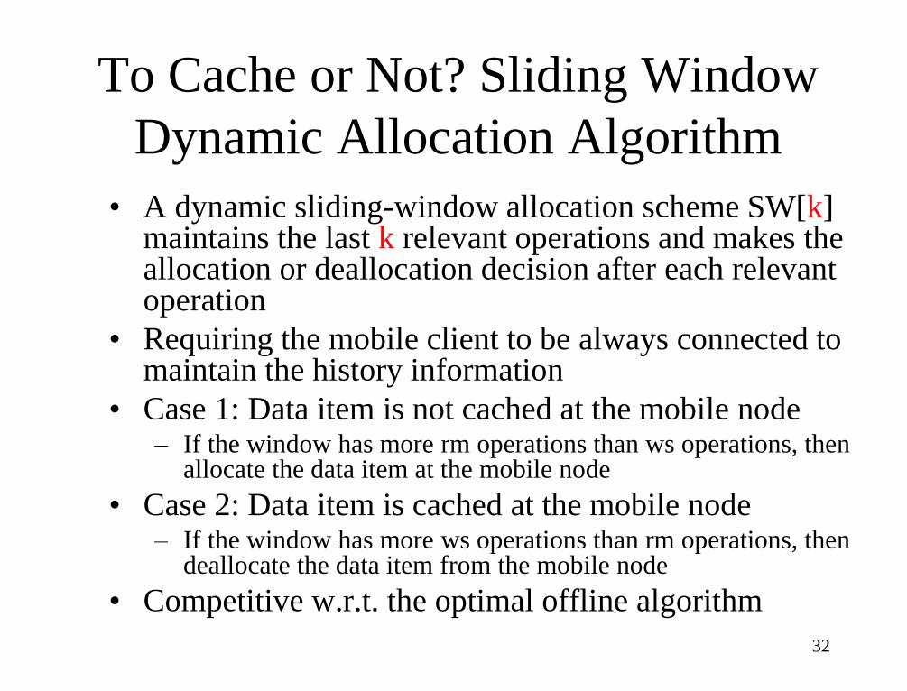
• A dynamic sliding-window allocation scheme SW[k] maintains the last k relevant operations and makes the allocation or deallocation decision after each relevant operation

• Requiring the mobile client to be always connected to maintain the history information

• Case 1: Data item is not cached at the mobile node – If the window has more rm operations than ws operations, then

allocate the data item at the mobile node

• Case 2: Data item is cached at the mobile node – If the window has more ws operations than rm operations, then

deallocate the data item from the mobile node

• Competitive w.r.t. the optimal offline algorithm

33

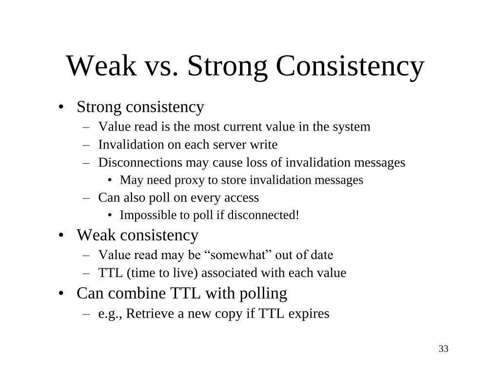
Weak vs. Strong Consistency

• Strong consistency – Value read is the most current value in the system

– Invalidation on each server write

– Disconnections may cause loss of invalidation messages

• May need proxy to store invalidation messages

– Can also poll on every access

• Impossible to poll if disconnected!

• Weak consistency – Value read may be “somewhat” out of date

– TTL (time to live) associated with each value

• Can combine TTL with polling

– e.g., Retrieve a new copy if TTL expires

34

Invalidation Report for Strong

Cache Consistency • Stateless: Server does not maintain information about the

cache content of the clients – Synchronous: An invalidation report is broadcast periodically, e.g.,

the Broadcast Timestamp scheme

– Asynchronous: reports are sent on data modification

– Property: A client cannot miss an update (say because of sleep or disconnection); otherwise, it will need to discard the entire cache content

• Stateful: Server keeps track of the cache contents of its clients – Synchronous: does not exist

– Asynchronous: A proxy is used for each client to maintain state information for items cached by the client and their last modification times; invalidation messages are sent to the proxy asynchronously.

– Clients can miss updates and get sync with the proxy (agent) upon reconnection

35

Asynchronous Stateful (AS) Scheme (Ref. [6])

• Whenever the server updates any data item, an invalidation report message is sent to the MH’s home location cache (HLC) maintained by the current Mobile Switching Station (MSS) which serves as the MH’s proxy – The MH’s HLC keeps track of data items cached by the MH.

– The HLC is a list of records (x,T,invalid_flag) for each data item x locally cached at MH where x is the data item ID and T is the timestamp of the last invalidation of x

– Invalidation reports are transmitted asynchronously and are buffered at the HLC until explicit acknowledgment is received from the specific MH. The invalid_flag is set to true for data items for which an invalidation message has been sent to the MH but no acknowledgment is received

• Before answering queries from application, a MH verifies whether a requested data item is in a consistent state with the HLC. If it is valid, it will satisfy the query; otherwise, an uplink request to the server is issued.

36

Asynchronous Stateful (AS) Scheme

• When the MH receives an invalidation message

from its MSS, it discards that cached data item

• In the sleep mode, the MH is unable to receive any

invalidation message

• When a MH reconnects, it sends a probe

message to its MSS with its cache timestamp

upon receiving a query. In response to this probe

message, the MSS sends an invalidation report.

• The AS scheme can handle arbitrary sleep patterns

of the MH.

37

Analysis of AS Scheme

• Performance Metrics:

– Cache miss probability

– Mean query delay

• Model constraints: A single Mobile

Switching Station (MSS) with N mobile

hosts

– This MSS is the server and also maintains the

home location cache (HLC) for all the MHs

(not a good assumption).

38

System Model of AS Scheme

• No query when MH is disconnected

• Single wireless channel of bandwidth C

• All messages are queued and serviced FCFS

• M data items, each of size ba bits

• A query is of size bq bits

• An invalidations report is of size bi bits

39

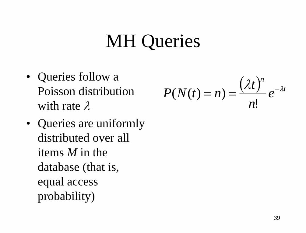
MH Queries

• Queries follow a

Poisson distribution

with rate l

• Queries are uniformly

distributed over all

items M in the

database (that is,

equal access

probability)

t

n

en

tntNP ll

!))((

40

Data Item Updates

• Time between two consecutive updates to a

data item is exponentially distributed with

rate μ

41

MH States

• Mobile hosts alternate between sleep and awake modes

• s is the fraction of time in sleep mode with 0 ≤ s ≤ 1

• Time between two consecutive wakeups is exponentially distributed with rate ω

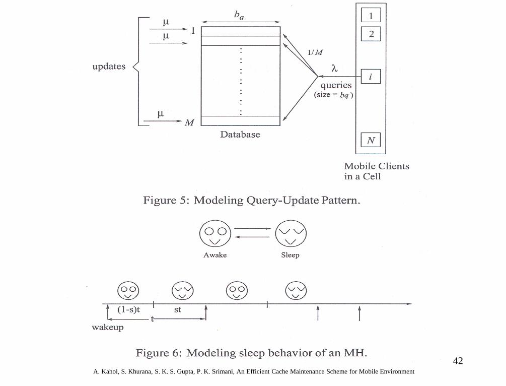
42 A. Kahol, S. Khurana, S. K. S. Gupta, P. K. Srimani, An Efficient Cache Maintenance Scheme for Mobile Environment

43

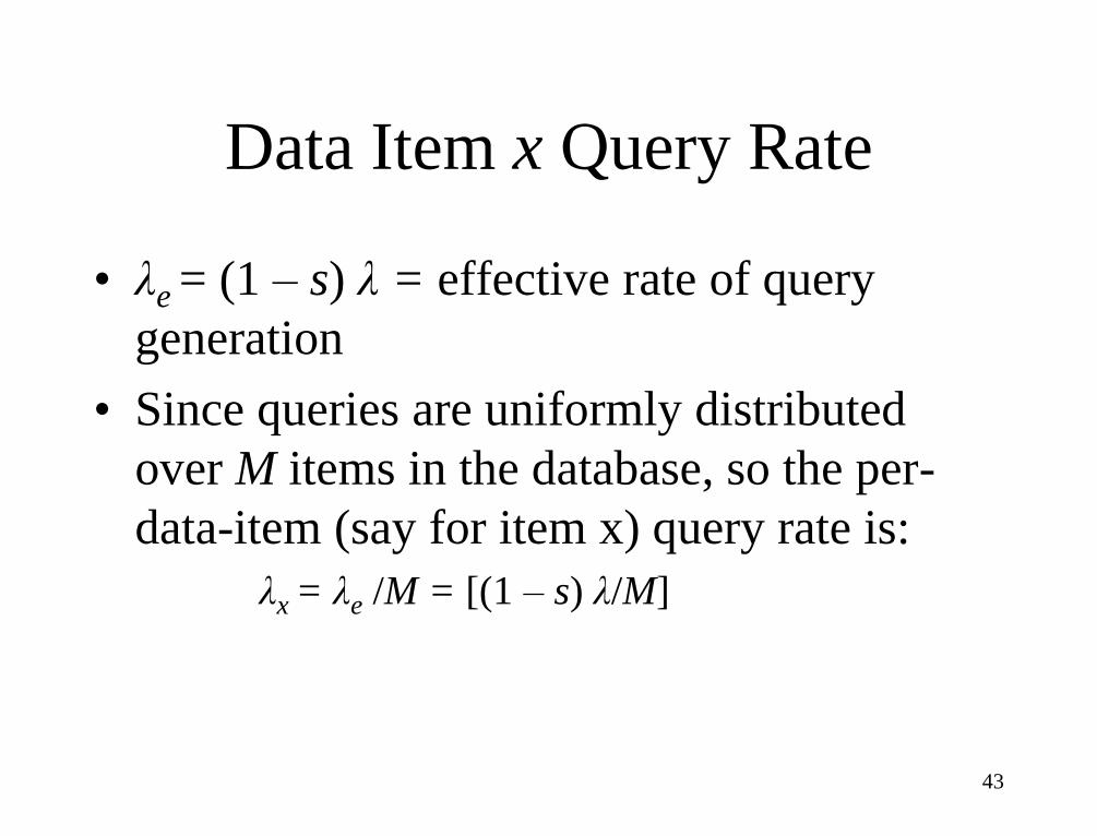
Data Item x Query Rate

• λe = (1 – s) λ = effective rate of query

generation

• Since queries are uniformly distributed

over M items in the database, so the per-

data-item (say for item x) query rate is:

λx = λe /M = [(1 – s) λ/M]

44

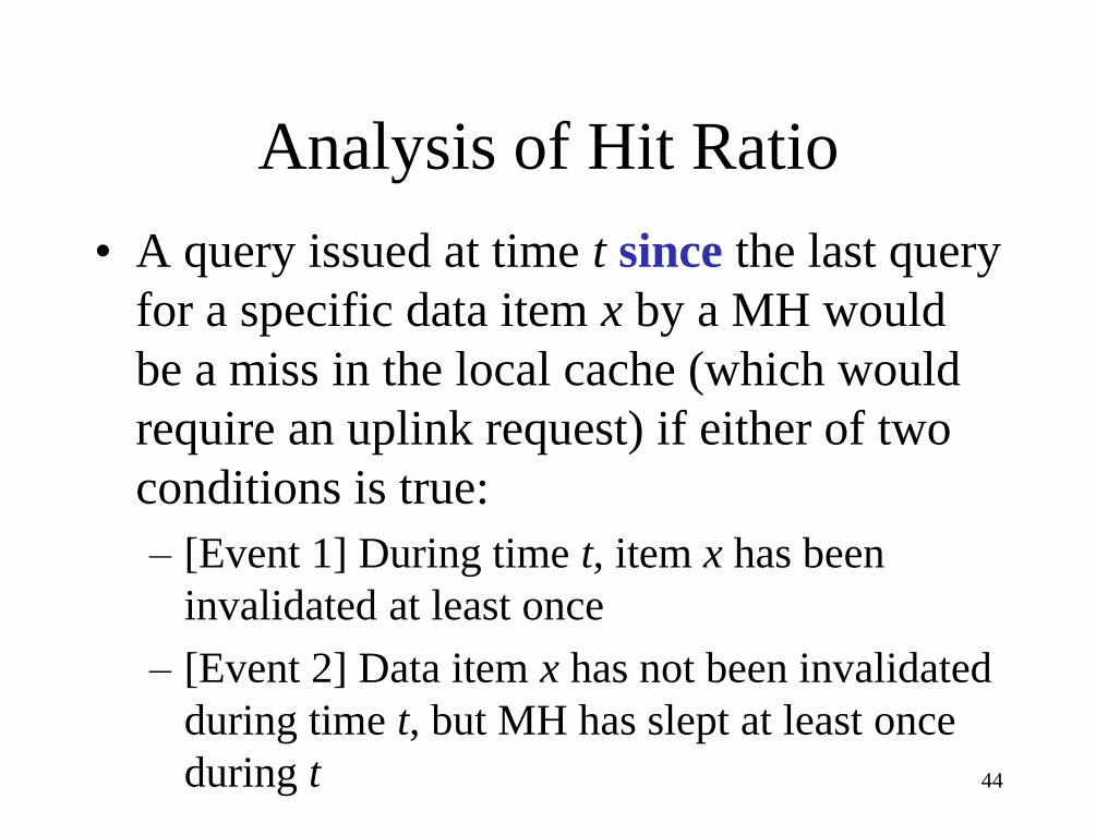
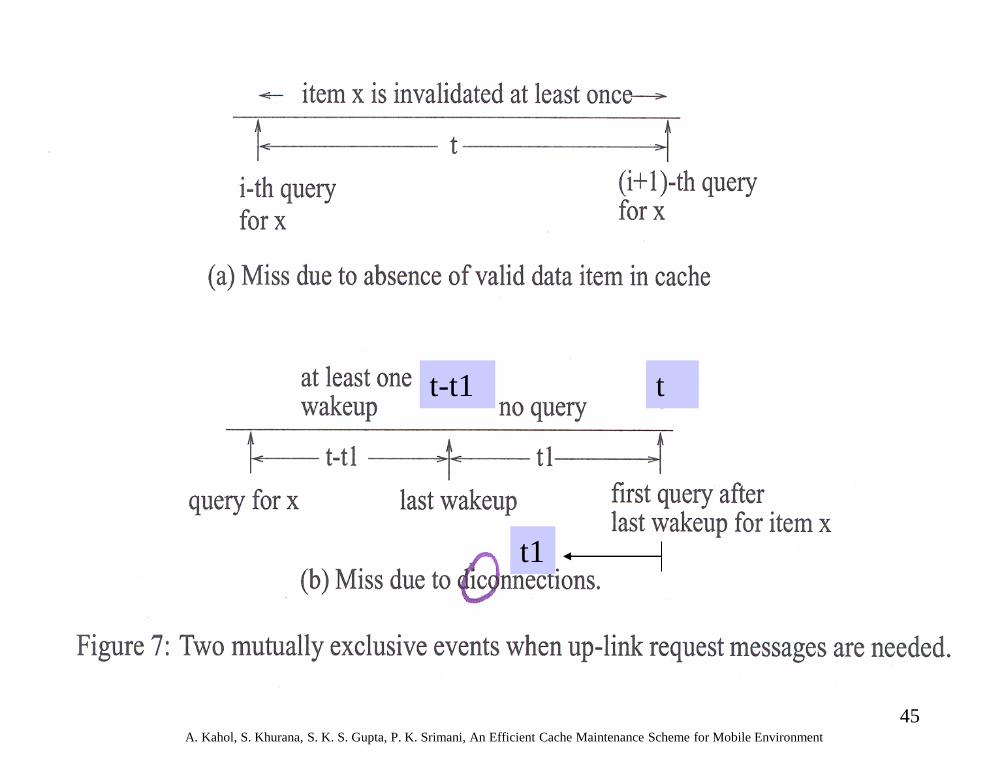
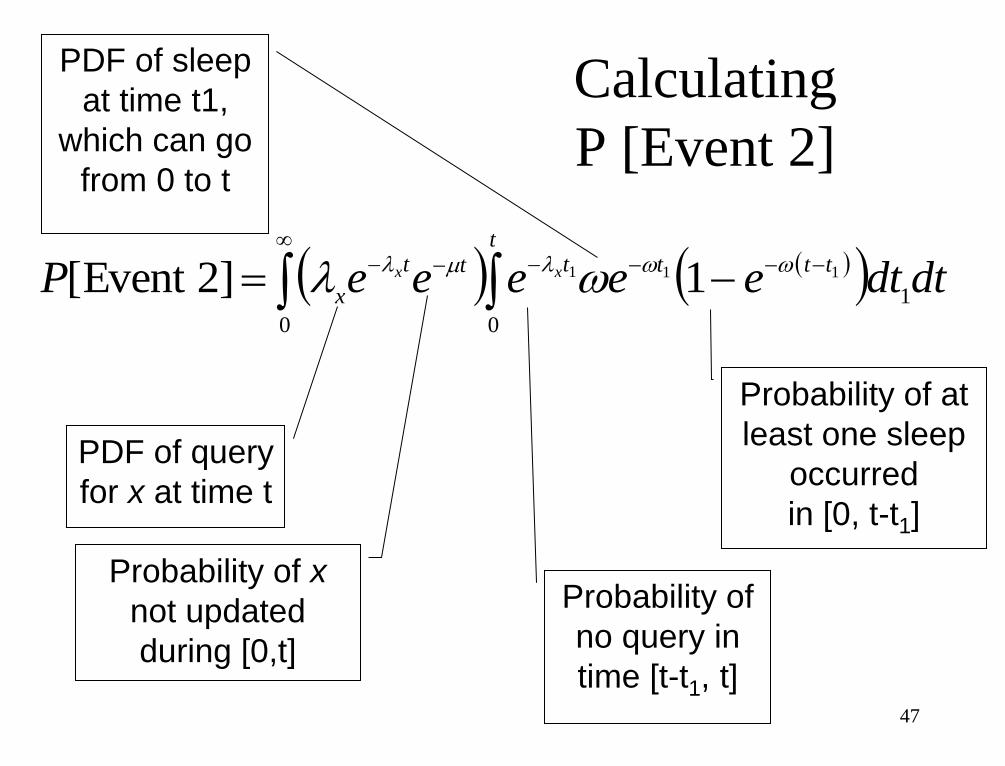
Analysis of Hit Ratio

• A query issued at time t since the last query

for a specific data item x by a MH would

be a miss in the local cache (which would

require an uplink request) if either of two

conditions is true:

– [Event 1] During time t, item x has been

invalidated at least once

– [Event 2] Data item x has not been invalidated

during time t, but MH has slept at least once

during t

45 A. Kahol, S. Khurana, S. K. S. Gupta, P. K. Srimani, An Efficient Cache Maintenance Scheme for Mobile Environment

t-t1 t

t1

46

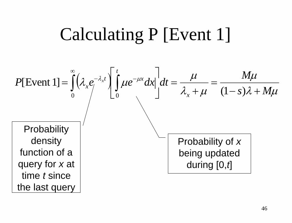
Calculating P [Event 1]

0 0)1(

]1Event [ml

m

ml

mml ml

Ms

MdtdxeeP

x

t

xt

xx

Probability

density

function of a

query for x at

time t since

the last query

Probability of x

being updated

during [0,t]

47

0 0

1

111 1]2Event [t

tttttt

xdtdteeeeeP xx lml l

PDF of query

for x at time t

Probability of x

not updated

during [0,t]

Probability of

no query in

time [t-t1, t]

PDF of sleep

at time t1,

which can go

from 0 to t

Probability of at

least one sleep

occurred

in [0, t-t1]

Calculating

P [Event 2]

48

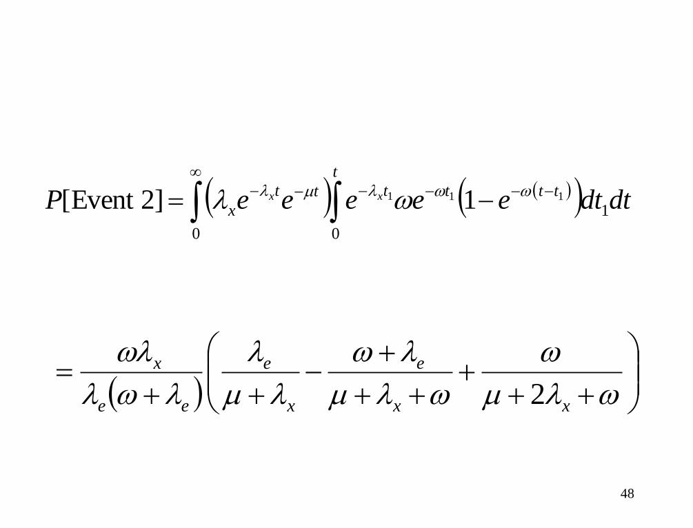
0 0

1111 1]2Event [

t

tttttt

x dtdteeeeeP xx lml l

lm

lm

l

lm

l

ll

l

xx

e

x

e

ee

x

2

49

Pmiss and Phit

• Pmiss = P[Event 1] + P[Event 2]

• Phit = 1 - Pmiss

50

Analysis of Mean Query Delay

• Let Tdelay be the mean query delay, then Tdelay = Phit *0 + PmissTq = PmissTq where Tq

is the uplink query delay

• Model the up-link query-response behavior as an M/D/1 queue

• Model the down-link invalidation message as another M/D/1 queue

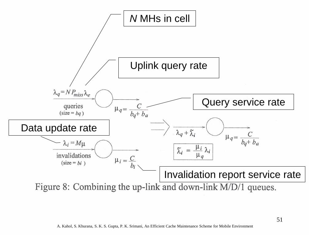
51 A. Kahol, S. Khurana, S. K. S. Gupta, P. K. Srimani, An Efficient Cache Maintenance Scheme for Mobile Environment

N MHs in cell

Uplink query rate

Query service rate

Invalidation report service rate

Data update rate

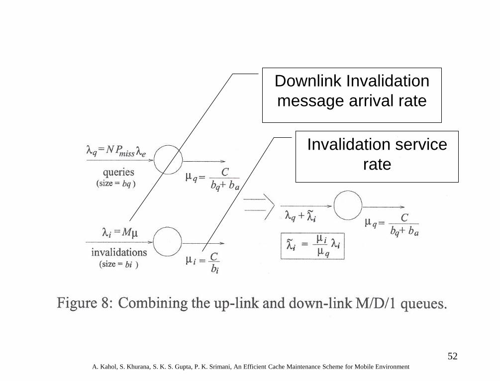
52 A. Kahol, S. Khurana, S. K. S. Gupta, P. K. Srimani, An Efficient Cache Maintenance Scheme for Mobile Environment

Downlink Invalidation

message arrival rate

Invalidation service

rate

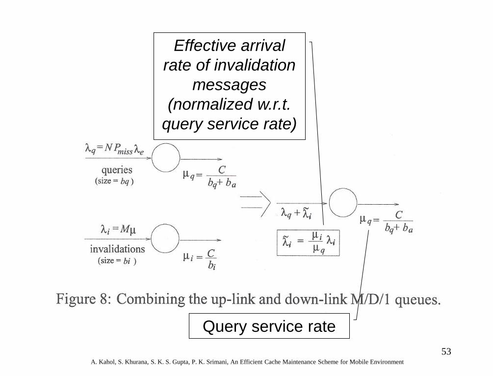
53 A. Kahol, S. Khurana, S. K. S. Gupta, P. K. Srimani, An Efficient Cache Maintenance Scheme for Mobile Environment

Effective arrival

rate of invalidation

messages

(normalized w.r.t.

query service rate)

Query service rate

54

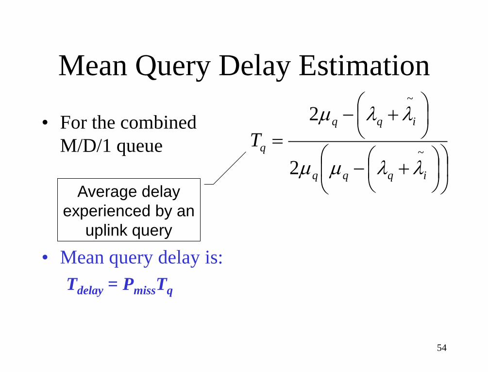
Mean Query Delay Estimation

• For the combined

M/D/1 queue

• Mean query delay is:

Tdelay = PmissTq

~

~

2

2

iqqq

iqq

qT

llmm

llm

Average delay

experienced by an

uplink query

55

References Chapter 3, F. Adelstein, S.K.S. Gupta, G.G. Richard III and L. Schwiebert, Fundamentals of Mobile and Pervasive Computing, McGraw Hill, 2005, ISBN: 0-07-141237-9.

Other References:

5. S. Lee, C.S. Hwang, and M. Kitsuregawa, “Efficient, Energy Conserving Transaction Processing in Wireless Data Broadcast,” IEEE Transactions on Knowledge and Data Engineering, Vol. 18, No. 9, Sept. 2006, pp. 1225-1238.

6. A. Kahol, S. Khurana, S.K.S. Gupta and P.K. Srimani, “A strategy to manage cache consistency in a disconnected distributed environment,” IEEE Transactions on Parallel and Distributed Systems, Vol. 12. No. 7, July 2001, pp. 686-700.