Lecture 2 Exercise 1awiki.ece.rose-hulman.edu/herniter/images/a/a9/MBSD... · Lecture 3A – Problem1 System Rise Time • We would like to redo our rise time measurement using the

1

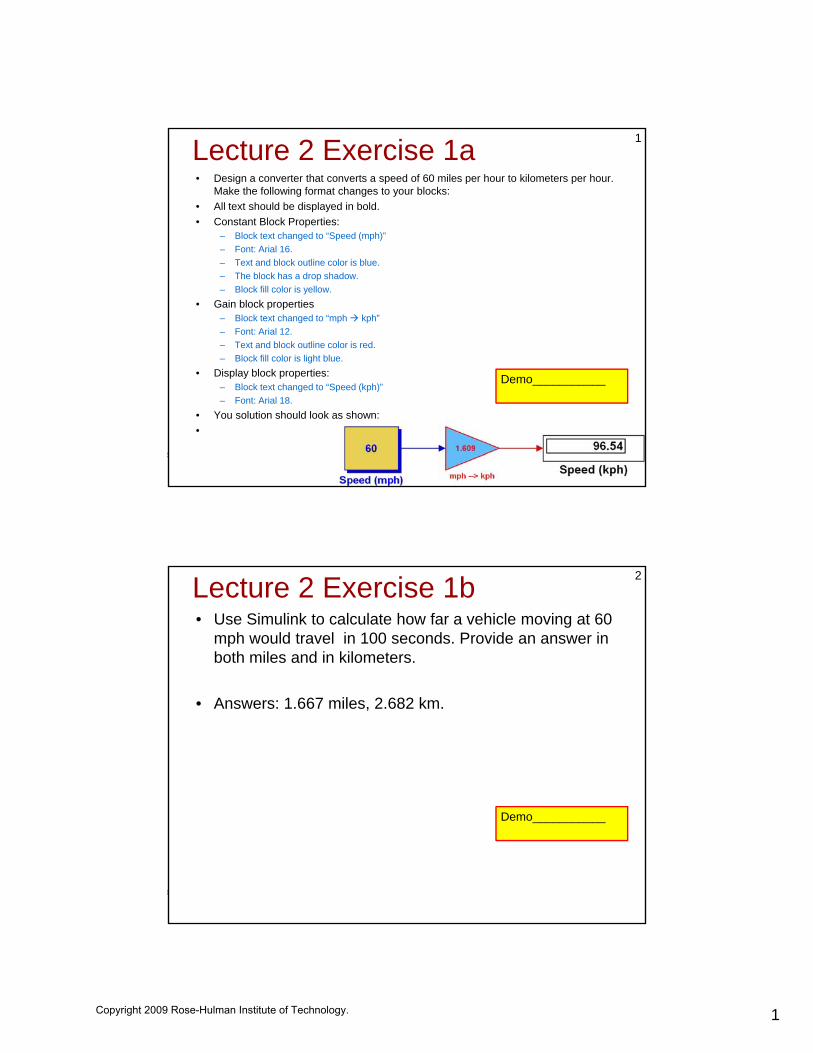
Lecture 2 Exercise 1a• Design a converter that converts a speed of 60 miles per hour to kilometers per hour.

Make the following format changes to your blocks:• All text should be displayed in bold.• Constant Block Properties:

– Block text changed to “Speed (mph)”Font: Arial 16

1

– Font: Arial 16.– Text and block outline color is blue.– The block has a drop shadow.– Block fill color is yellow.

• Gain block properties– Block text changed to “mph kph”– Font: Arial 12.– Text and block outline color is red.– Block fill color is light blue.

• Display block properties:– Block text changed to “Speed (kph)”– Font: Arial 18.

• You solution should look as shown:•

Demo___________

Lecture 2 Exercise 1b• Use Simulink to calculate how far a vehicle moving at 60

mph would travel in 100 seconds. Provide an answer in both miles and in kilometers.

2

• Answers: 1.667 miles, 2.682 km.

Demo___________

Copyright 2009 Rose-Hulman Institute of Technology.

2

Lecture 2 Exercise 2Modify the motor model to use the name

plate specifications for the motors and generators used in the lab Use the

3

generators used in the lab. Use the following items listed on the nameplate:• Torque constant.• Rotor Inertia.

• Max motor current is 6.3 amps. (Due to current limits on the DC power supply.)

Demo___________

Lecture 2 Exercise 3• Verify the operation of your

generator model.• Copy the Generator

subsystem to a new model

4

Demosubsystem to a new model.• Generate a plot of generator

load torque versus shaft rpm.

• You should obtain a plot as shown below:

Demo___________

shown below:• You may need to add a part

called SimDriveline Env to get your simulation to run.


3

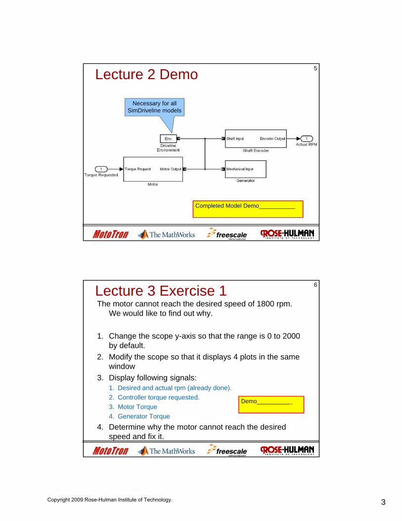
Lecture 2 Demo 5

Necessary for all SimDriveline models

Completed Model Demo___________

Lecture 3 Exercise 1The motor cannot reach the desired speed of 1800 rpm.

We would like to find out why.

1. Change the scope y-axis so that the range is 0 to 2000

6

g p y gby default.

2. Modify the scope so that it displays 4 plots in the same window

3. Display following signals:1. Desired and actual rpm (already done). 2 Controller torque requested2. Controller torque requested.3. Motor Torque4. Generator Torque

4. Determine why the motor cannot reach the desired speed and fix it.

Demo___________


4

Lecture 3 Demo 1Verification – Controller Gain

7

• Test 3 - Set controller gain to 0.001– Steady state error (rpm) __________________– Steady state stability __________________

• Test 4 – Set controller gain to 0.01– Steady state error (rpm) __________________– Steady state stability __________________

• Test 5 – Set controller gain to 0.1– Steady state error (rpm) DemoSteady state error (rpm) __________________– Steady state stability __________________

• Test 6 – Set controller gain to 1– Steady state error (rpm) __________________– Steady state stability __________________

Demo___________

Lecture 3 Exercise 2• Verify the operation of

your motor model.• Copy the Motor

subsystem to a new

8

Demo___________

subsystem to a new model.

• Generate a plot of motor torque versus shaft rpm.

• You should obtain a plot as shown:as shown:

• You may need to add a part called SimDriveline Env to get your simulation to run.


5

Lecture 3 Demo 2 Verification – Feedback Gain

• Test 4 - Set controller gain to 0.001 Old Model New Model– Steady state error (rpm) ___________ ___________– Torque Signal ___________ ___________

9

– Steady state stability ___________ ___________• Test 5 – Set controller gain to 0.01

– Steady state error (rpm) ___________ ___________– Torque Signal ___________ ___________– Steady state stability ___________ ___________

• Test 6 – Set controller gain to 0.1– Steady state error (rpm) ___________ ___________– Torque Signal ___________ ___________– Steady state stability ___________ ___________

• Test 7 – Set controller gain to 1– Steady state error (rpm) ___________ ___________– Torque Signal ___________ ___________– Steady state stability ___________ ___________

Demo___________

Lecture 3 Demo 3 Verification – Generator IC

• Test 1 - Set IC to 0 rad/s, all else constant– Old Model

10

Old Model __________________________– New Model __________________________

• Test 2 – Set IC to 250 rad/s, all else constant– Old Model __________________________– New Model __________________________

Th lt h ld t h i• These results should match our previous simulations since 6 bulbs is equivalent to what we did previously.

Demo___________


6

Lecture 3 Demo 4 Verification – FeedbackGain

• Test 4 - Set controller gain to 0.001 Old Model New Model– Steady state error (rpm) ___________ ___________– Torque Signal ___________ ___________

11

– Steady state stability ___________ ___________• Test 5 – Set controller gain to 0.01

– Steady state error (rpm) ___________ ___________– Torque Signal ___________ ___________– Steady state stability ___________ ___________

• Test 6 – Set controller gain to 0.1– Steady state error (rpm) ___________ ___________– Torque Signal ___________ ___________– Steady state stability ___________ ___________

• Test 7 – Set controller gain to 1– Steady state error (rpm) ___________ ___________– Torque Signal ___________ ___________– Steady state stability ___________ ___________

Demo___________


• Test 1 - Set number of bulbs to 0– Steady state error (rpm) ___________________________– Torque Signal ___________________________

12





Demo___________


7



13


• The results should show that the steady state error increases as we increase the number of bulbs.

• With no load (0 bulbs) the error should be very ( ) yclose to zero.

Demo___________



14





Demo___________


8



15


• The results should show that the steady state error increases as we increase the number of bulbs.

• With no load (0 bulbs) the error should be very ( ) yclose to zero.

• With 6 bulbs, the generator loads down the motor, and then motor cannot achieve the desired speed.

Demo___________

Lecture 3 Problem 1• Measure the step response of the motor so that we can

verify the quick response of the motor. You should obtain a plot similar to the one shown below.

16

Complete___________p ___________


herniter

Rectangle

9

Lecture 3 Problem 2• Capacitor Car – Description on next page.

17

Grade______________________

Lecture 3A Exercise 1• Use the fixed-step ode3 (Bokacki-Shampine) solver and

determine the largest fixed step size that can be used to simulate the system with out yielding an oscillation in the motor torque or plant rpm.

18

• The desired rpm should be set to 1800, number of bulbs to 3, and the feedback gain to 0.01 (same as used in the previous slides.)

• Note that when we deploy the controller on the MPC555x target, a fixed step size will be used. Thus, this is a good test to determine the required step size needed for our controller.q p

• Find the max step size to the nearest 100 µs.

Demo___________


10

ResultsLecture 3A Demo 1

19

Demo___________

Lecture 3A Exercise 2• Add the flywheel inertia to your system. (Repeat exercise 1 with

the added inertia.)• Use the fixed-step ode3 (Bokacki-Shampine) solver and

determine the largest fixed step size that can be used to

20

g psimulate the system with out yielding an oscillation in the motor torque or plant rpm.

• The desired rpm should be set to 1800, number of bulbs to 3, and the feedback gain to 0.01 (same as used in the previous slides.)

• Note that when we deploy the controller on the MPC555xNote that when we deploy the controller on the MPC555x target, a fixed step size will be used. Thus, this is a good test to determine the required step size needed for our controller.

• Find the max step size to the nearest 1 ms.

Demo___________


11

Lecture 3A – Problem1System Rise Time

• We would like to redo our rise time measurement using the motor generator system with the added flywheel.

• A second Speedgoat real-time system has been set up to

21Demo___________

control and measure data from the motor generator system:– The IP address is xxx.xxx.85.112.– The rpm signal conversion is 1.25 V per 1000 rpm. (We added a voltage

divider to cut the rpm signal in half.)

• Repeat the measurements of Lecture 3A Demo1 for the Motor-Generator system with a flywheel. Note that this system is

b bl 50 100 i l h h i lfprobably 50 to 100 times slower than the motor itself.• Generate a plot, calculate the time constant, and calculate the

rise time.• Note that this system is wired differently than the motor.

Lecture 3A – Problem2Measured Coast Down

• We would like to measure the coast-down response of the motor-generator system used in Problem 1.

• Let the motor speed up to its maximum speed and then allow

22Demo___________

the motor to coast to a stop.• For the coast-down, measure:

– The time constant.– The time it takes to reach zero (5 time constants)– Generate a plot of the coast-down response showing with the 10% and

90% points marked.

• Save the coast-down data in a file on your computer for use in a later example.


12

Lecture 4 Problem 1• Repeat the bode plot for our system and include the

flywheel inertia of 1.041×10-4 kg·m2.• Fill in the table below and generate a plot.

23

F ( d/ ) O t t A lit d G i G i (dB)

Demo___________

Frequency (rad/sec) Output Amplitude Gain Gain (dB)

0.1

1

2

4

8

10

20

40

80

100

1000

10000

Lecture 4 Problem 2A plant has the following transfer function

24

( )( )( )100111.011000

sss +++

We will use this plant with proportional feedback as shown in class.a) Use gain and phase plots to find the largest value of the feedback constant F

that can be used to have a stable system with zero degrees phase margin.b) Use Simulink to show that the system is unstable for values of F larger than

this value of F.c) Use Simulink to show that the system is stable for values less than or equal

to this value of F.d) Use gain and phase plots to find the largest value of the feedback constant F

that can be used to have a stable system with a 60 degrees phase margin.Grade___________


13

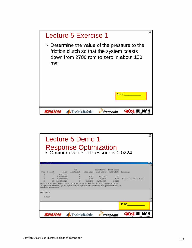
Lecture 5 Exercise 1• Determine the value of the pressure to the

friction clutch so that the system coasts down from 2700 rpm to zero in about 130

25

down from 2700 rpm to zero in about 130 ms.

Demo___________

Lecture 5 Demo 1Response Optimization• Optimum value of Pressure is 0.0224.

26

Demo___________


14

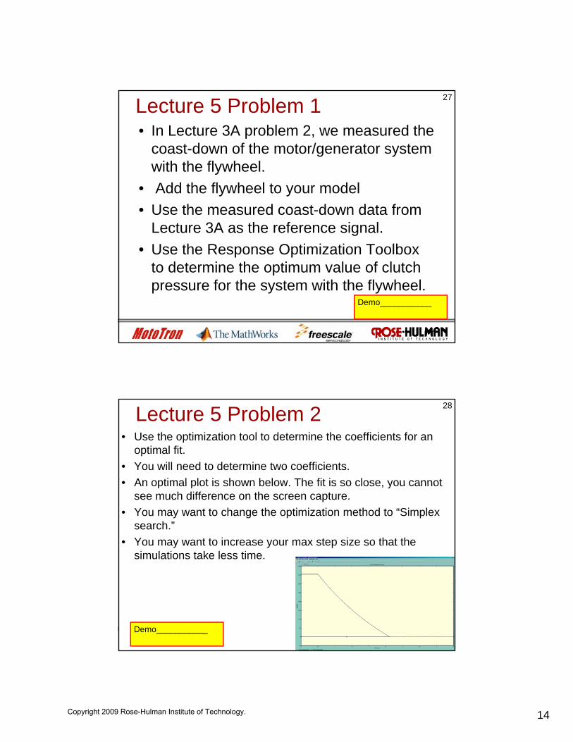
Lecture 5 Problem 1• In Lecture 3A problem 2, we measured the

coast-down of the motor/generator system with the flywheel.

27

y• Add the flywheel to your model• Use the measured coast-down data from

Lecture 3A as the reference signal.• Use the Response Optimization Toolbox

to determine the optimum value of clutch pressure for the system with the flywheel.

Demo___________

Lecture 5 Problem 2• Use the optimization tool to determine the coefficients for an

optimal fit.• You will need to determine two coefficients.• An optimal plot is shown below The fit is so close you cannot

28

• An optimal plot is shown below. The fit is so close, you cannot see much difference on the screen capture.

• You may want to change the optimization method to “Simplex search.”

• You may want to increase your max step size so that the simulations take less time.

Demo___________

Demo___________


15

Lecture 6 Demo 1• Demonstrate the system response for

various feedback gains.• Demonstrate the effect of reducing the

29

• Demonstrate the effect of reducing the simulation maximum step size,

DemoDemo___________

Init File- Lecture 6 Demo 2• Run your model now

It k b th I it Fil b f

30

Demo___________

• It works because the Init_File runs before the model runs, and defines all of the constants needed by the mode.

• From now on, we will define all of our data and model constants in the init file.and model constants in the init file.

• The model will reference the variables named in the init file rather than use magic numbers.


16

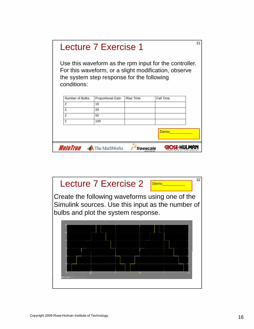
Lecture 7 Exercise 1 31

Use this waveform as the rpm input for the controller. For this waveform, or a slight modification, observe the system step response for the following

Number of Bulbs Proportional Gain Rise Time Fall Time

2 10

2 20

2 50

the system step response for the following conditions:

2 50

2 100

Demo___________

Lecture 7 Exercise 2Create the following waveforms using one of the Simulink sources. Use this input as the number of bulbs and plot the system response

32Demo___________

bulbs and plot the system response.


17

Lecture 7 Exercise 3Determine the maximum value of Sample time that can be used to achieve a stable feedback system using the conditions

33Demo___________

feedback system using the conditions specified below:

No Bulbs 1 Bulb 2 Bulbs 3 Bulbs

Gain = 10

Gain = 20

Gain = 50

Gain = 100

Lecture 7 Demo 1• Demo your PI controller.• Show how changing the P and I gains

affect the system response

34

affect the system response.

Demo___________


18

Lecture 7 Exercise 4 • Repeat the previous procedure for different values of

proportional gain.• Determine the proportional and integral gains to achieve a plot

close to the one below

35Demo___________

close to the one below.

Lecture 7 Demo 2• Demo your PI controller with 1 bulb load.• Show how changing the P and I gains

affect the system response

36

affect the system response.• Determine values of P and I gains for

optimum response.

Demo___________


19

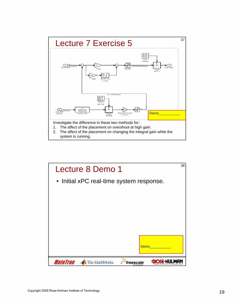
Lecture 7 Exercise 5 37

Investigate the difference in these two methods for:1. The affect of the placement on overshoot at high gain.2. The affect of the placement on changing the integral gain while the

system is running.

Demo___________

Lecture 8 Demo 1• Initial xPC real-time system response.

38

Demo___________


20

Lecture 8 Demo 2• Constant speed, variable load testing.

39

Demo___________

Lecture 8 Demo 3• System response for constant load,

constant speed, variable feedback gain.

40

Demo___________


21

Lecture 9 Problem 1• The plots demonstrated in this lecture were for our motor-

generator system without the flywheel.• For the problems in this section, we would like to use the

transfer function from the system with the flywheel

41

transfer function from the system with the flywheel.• In lecture 4 problem 1, we measured the frequency response

plot of the motor-generator system including the flywheel.• Determine the transfer function of this system from the

measured frequency plot.• Show the magnitude frequency plot whence your transfer

function was generated.

Answer___________

Lecture 9 Problem 2• For a feedback gain of 1, determine the largest fixed

time step where the system will be stable (0.1, 0.01, 0.001, 0.0001)

42

• Show gain and phase plots using Matlab.• The plots should be displayed in the same manner as

shown in the notes for lecture 9.

Gain and plots___________


22

Lecture 9 Problem 3• For a feedback gain of 10, determine the largest fixed

time step where the system will be stable (0.1, 0.01, 0.001, 0.0001)

43




Lecture 9 Problem 4• For a feedback gain of 100, determine the largest

fixed time step where the system will be stable (0.1, 0.01, 0.001, 0.0001)

44





23

Lecture 10 xPC 1• Obtain a copy of the next screen using the

xpctargetspy command.

45

XPCTARGETSPY



46

XPCTARGETSPY


24



47

XPCTARGETSPY

Lecture 10 Gauges - Demo• Demonstrate your working model to me.

– Front Panel DisplayxPC Real-Time Display

48

– xPC Real-Time Display

Demo___________


25

Lecture 10A Demo 1• Demonstrate the controller as an atomic

subsystem with sample times of 0.1, 0.01, and 0 001 seconds

49

and 0.001 seconds.

Demo___________

Lecture 10A Demo 2 50

Demo___________


26

Lecture 11 Exercise 1• Change the LED flasher frequency to 2 Hz

and demonstrate your working system.

51

Demo___________

Lecture 11 Exercise 2• Create an 8-Bit ring counter that changes

state every ½ second.• Do not use Stateflow to do this

52

• Do not use Stateflow to do this.• The LED output sequence is shown below:

1 0 0 0 0 0 0 00 1 0 0 0 0 0 00 0 1 0 0 0 0 00 0 0 1 0 0 0 00 0 0 0 1 0 0 00 0 0 0 0 1 0 00 0 0 0 0 0 1 00 0 0 0 0 0 0 1

Demo___________


27

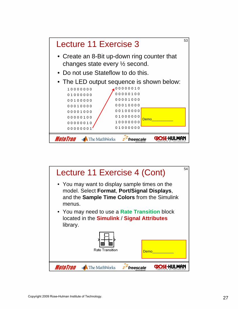
Lecture 11 Exercise 3• Create an 8-Bit up-down ring counter that

changes state every ½ second.• Do not use Stateflow to do this

53

• Do not use Stateflow to do this.• The LED output sequence is shown below:

1 0 0 0 0 0 0 00 1 0 0 0 0 0 00 0 1 0 0 0 0 00 0 0 1 0 0 0 0

0 0 0 0 0 0 1 00 0 0 0 0 1 0 00 0 0 0 1 0 0 00 0 0 1 0 0 0 0

0 0 0 0 1 0 0 00 0 0 0 0 1 0 00 0 0 0 0 0 1 00 0 0 0 0 0 0 1

0 0 1 0 0 0 0 00 1 0 0 0 0 0 01 0 0 0 0 0 0 00 1 0 0 0 0 0 0

Demo___________

Lecture 11 Exercise 4 (Cont)• You may want to display sample times on the

model. Select Format, Port/Signal Displays, and the Sample Time Colors from the Simulink

54

menus. • You may need to use a Rate Transition block

located in the Simulink / Signal Attributes library.

Demo___________


28

Lecture 11A Demo 1 • Repeat the Procedure to display the values of

signals Repeating_Sequence_Fast and Sequence:

55Demo___________

• You should see the fast and slow signals change• You should see the fast and slow signals change at different rates, and the Sequence signal should flip-flop between the fast and slow rates.

Lecture 11A Demo 2 56Demo___________


29

Lecture 11A Problem 1• Create the following display of information:

57Demo___________

Lecture 11A Problem 2• Create the plot shown on the next page.

Note that only bits 0 through 6 are shown.

58Demo___________


30

Lecture 12 Problem 1• Determine the decimal value of the following

bit string (it is 32 bits in length.)• 10011100111011100110111000000011

59

• 10011100111011100110111000000011• Assuming the following data types

– Uint32 (magnitude)– Int32 (2’s complement)– Sign and magnitudeg g– Single precision floating point

• Create an m-file that displays all four results in an mbox.

Lecture 12 Problem 2• Determine the decimal value of the following

bit string (it is 32 bits in length.)• 01000000111010000110100000000011

60

• 01000000111010000110100000000011• Assuming the following data types

– Uint32 (magnitude)– Int32 (2’s complement)– Sign and magnitudeg g– Single precision floating point

• Create an m-file that displays all four results in an mbox.


31

Lecture 12 Problem 3• Create an m-file that defines a arbitrary 32 character

text string, the contents of which are zeros and ones. For example,

61

‘01000000111010000110100000000011’• The script then displays the value of the bit string in an

mbox, assuming the four data types below:– Uint32 (magnitude)– Int32 (2’s complement)– Sign and magnitude– Single precision floating point

• Demonstrate your function with a binary value given by your instructor.

Lecture 12 Exercise 1• Create an counter that changes state every ½ second.• Do not use Stateflow to do this.• The repeating LED output sequence is shown below:

62

The repeating LED output sequence is shown below:

0 0 0 0 0 0 0 01 0 0 0 0 0 0 01 1 0 0 0 0 0 01 1 1 0 0 0 0 0

1 1 1 1 1 1 1 10 1 1 1 1 1 1 10 0 1 1 1 1 1 10 0 0 1 1 1 1 1

1 1 1 1 0 0 0 01 1 1 1 1 0 0 01 1 1 1 1 1 0 01 1 1 1 1 1 1 0

0 0 0 0 1 1 1 10 0 0 0 0 1 1 10 0 0 0 0 0 1 10 0 0 0 0 0 0 1

Demo___________


32

Lecture 12 Exercise 2• Create an counter that changes state every ½

second.• Do not use Stateflow to do this.

63

• The repeating LED output sequence is shown below:

0 0 0 0 0 0 0 01 0 0 0 0 0 0 01 1 0 0 0 0 0 01 1 1 0 0 0 0 0

1 1 1 1 1 1 1 11 1 1 1 1 1 0 01 1 1 1 1 0 0 01 1 1 1 0 0 0 0

1 1 1 1 0 0 0 01 1 1 1 1 0 0 01 1 1 1 1 1 0 01 1 1 1 1 1 1 0

1 1 1 0 0 0 0 01 1 0 0 0 0 0 01 0 0 0 0 0 0 0

Demo___________

Lecture 13 – Demo 1• Wire up your circuit.• Modify the model to display the value of

the digital input and the count using the

64

the digital input and the count using the FreeMaster tool.

• Compile and download the model.• Demo your working system.

– The ring counter should change directionThe ring counter should change direction when the push-button is pressed.

Demo___________


33

Lecture 13 - Demo 2Mod 8 counter using a triggered subsystem.• Wire up your circuit.• Use the FreeMASTER tool to monitor the following signals for

the triggered subsystem:

65Demo___________

gg y– The input.– The output– The switch output– The output of the 1/z block– The trigger– An example display is shown on the next slide.

• Compile and download the model.• Demo your working system.• The counter should hold when you press the pushbutton.

Lecture 13 Exercise 1• You will notice that the counter does hold when

press the bust-button. However, there is a problem:

66

• When the count reaches 7 and you press the hold push button, all of the LEDs go out and the count holds (actually at -1).

• Fix this problem so that the count always holds when the button is pushed, the counter always remembers the count, and there is one LED on at all times.

Demo___________


34

Lecture 13 Exercise 2a• Create an up-down ring counter that changes

direction when you press a push-button. (A hold button is not required).

67Demo___________

– When the push-button is not depressed, the ring counter goes in the “normal” direction.

– While the push-button is depressed, the ring counter goes in the opposite direction

• The counter should not skip or jump when you press the button (the count should bepress the button (the count should be continuous).

• You are required to use a triggered subsystem to solve this problem.

Lecture 13 Exercise 2b• Create an up-down ring counter that changes direction

when you press a push-button. (A hold button is not required).

• The push button has memory (similar to a flip flop):

68Demo___________

• The push-button has memory (similar to a flip-flop):– When the push-button is pressed and released, the counter

changes direction.– The counter does not change direction until the push-button is

pressed and released again.– The counter changes direction every time the push-buton is

pressed and then released.

• The counter should not skip or jump when you press the button (the count should be continuous).

• You are required to use a triggered subsystem to solve this problem.


35

Lecture 13 Exercise 3• Create an up-down ring counter that changes

direction when you press a push-button. (A hold button is not required).

69

• The counter should not skip or jump when you press the button. (The count should be continuous).

• A second push-button should be used to change the counting frequency. You should be able to change directions and speed simultaneously.

Demo___________

Lecture 13 Exercise 4• Create two 4-bit ring counters with the following

properties:– One counter shifts to the right, the other shifts to the left.

One counter counts at a 1 Hz rate the other at a 10 Hz rate

70

– One counter counts at a 1 Hz rate, the other at a 10 Hz rate.– Your fixed step size is 1 ms.– Two push-buttons are available that hold the individual counters.

While holding, the counters cannot lose their count. The hold functions on each counter are independent of the other counter.

• You are required to use triggered subsystem to solve this problem.

Demo___________


36

Lecture 14 – Demo 1• Analog Input – Demo• Wire up you circuit.• Compile and download the model.

71

• Display all signal values using FreeMASTER:• Demo your working analog voltmeter / bar graph.

Demo___________

Lecture 14 – Demo 2• Wire up you circuit.• Compile and download the model.

D ki t

72

• Demo your working system.– Ring counter with embedded Matlab function.

Demo___________


37

Lecture 14 Exercise 1• Create an up-down ring counter where the

up/down function and the ring counting logic is contained in an Embedded MATLAB Function

73Demo___________

block.• As push-button is used to change directions of

the counter.• The counter is allowed to skip positions when

you press the push-button.• You may use a counter external to the

embedded Matlab function if you so desire.

Lecture 14 Exercise 2• Create an up-down ring counter where the up/down

function, the ring counting logic, and the stored count is contained in an Embedded MATLAB Function block.

• As push button is used to change directions of the

74Demo___________

• As push-button is used to change directions of the counter.

• The counter is not allowed to skip positions when you press the push-button.

• The embedded function must keep track of the count. You may not use an external counter to keep track of the

t (I th b dd d M tl b f ti hcount. (In essence, the embedded Matlab function has memory.)– You may want to use the Matlab persistent and isempty

functions.


38

Lecture 14 Exercise 3• Create a ring counter using a Truth Table.

• Truth Tables are located in the Stateflow library

75

Truth Tables are located in the Stateflow library.

Demo___________

Lecture 14 Demo 3• Wire up you circuit.• Compile and download the model.

D ki t

76

• Demo your working system.– Analog voltmeter with ASCII output.

Demo___________


39

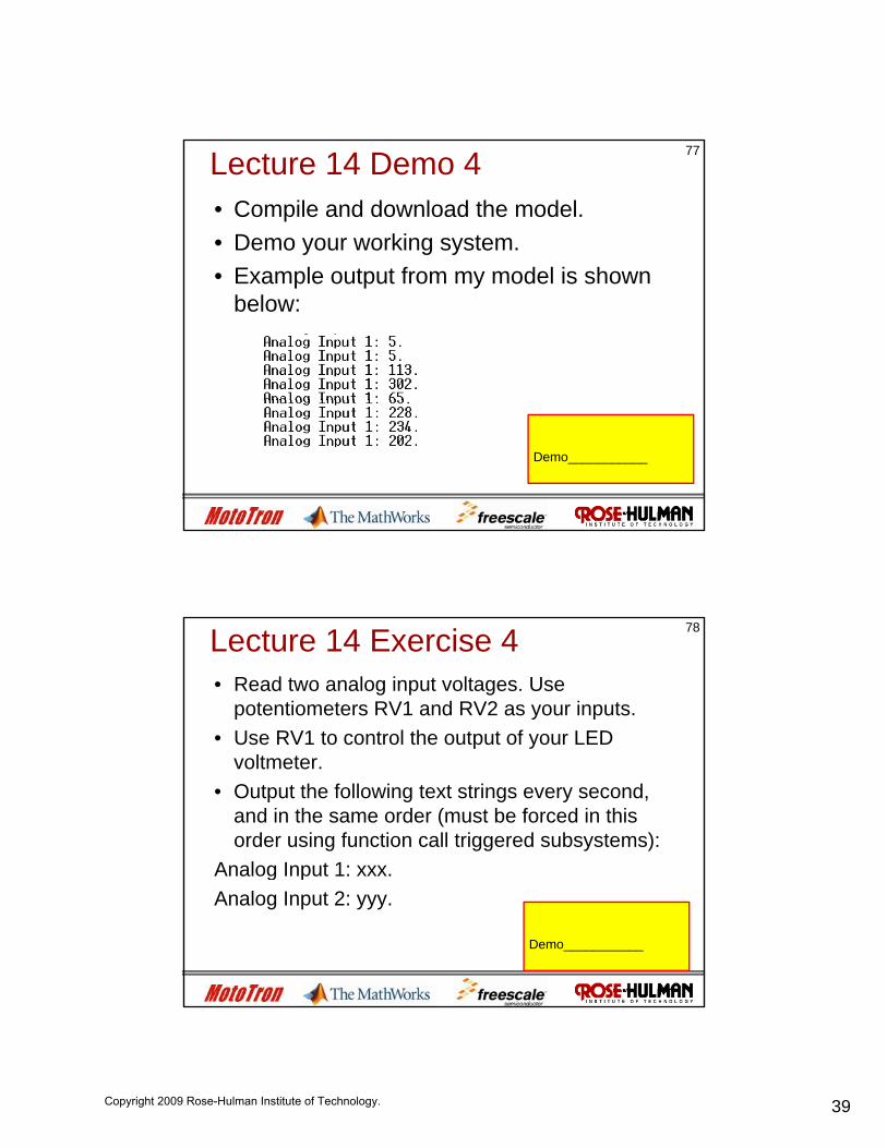
Lecture 14 Demo 4• Compile and download the model.• Demo your working system.

E l t t f d l i h

77

• Example output from my model is shown below:

Demo___________

Lecture 14 Exercise 4• Read two analog input voltages. Use

potentiometers RV1 and RV2 as your inputs.• Use RV1 to control the output of your LED

78

p yvoltmeter.

• Output the following text strings every second, and in the same order (must be forced in this order using function call triggered subsystems):

Analog Input 1: xxx.g pAnalog Input 2: yyy.

Demo___________


40

Lecture 14 Exercise 5• Use the analog input and a potentiometer to

control the speed at which your ring counter shifts.

79

• The counter frequency should be continuously variable from 1 Hz to 10 Hz.

Demo___________

Lecture 14A Problem1 80Demo___________

This text goes bright if the value goes above 448.

This value is always underlined.


41

Lecture 14A Problem2• We would like to create a new subsystem block that

displays text with the following characteristics.• The input to the block is a numerical value of type

double

81Demo___________

double.• The block should be a masked subsystem that specifies:

– The row and column where the block is placed on the screen.– The text displayed on the screen before the numerical value.– The period in milliseconds at which the numerical value is

refreshed.– Two threshold values:– Two threshold values:

• When the numerical value is below Threshold1, the text is displayed in black.

• When the numerical value is between Threshold1 and Threshold2, the text is underlined.

• When the numerical value is above Threshold2, the text blinks.

Lecture 15 Demo 1• MPC555x eMIOS PWM Output• Verify that the frequency is 20 kHz and that

the duty cycle is 50%

82

the duty cycle is 50%.• Display waveforms of the PWM output with

the Mobile Studio Desktop Oscilloscope

Demo___________


42

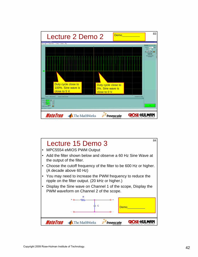
Lecture 2 Demo 2• Sine Wave Modulated PWM Waveform

83Demo___________

Duty cycle close to 100%. Sine wave is

Duty cycle close to 0%. Sine wave is

close to 5 V. close to 0 V.

Lecture 15 Demo 3• MPC5554 eMIOS PWM Output• Add the filter shown below and observe a 60 Hz Sine Wave at

the output of the filter. • Choose the cutoff frequency of the filter to be 600 Hz or higher.

84

q y g(A decade above 60 Hz)

• You may need to increase the PWM frequency to reduce the ripple on the filter output. (20 kHz or higher.)

• Display the Sine wave on Channel 1 of the scope, Display the PWM waveform on Channel 2 of the scope.

R

Demo___________

+

-

R

C

+

-


43

Lecture 15 Demo 41) Before connecting the motor, verify that

you can use the POT to control the output duty cycle (Display in the scope)

85

duty cycle. (Display in the scope)

Verify this signal.

Demo___________

Motor Control Demo 52) Once you have verified the PWM signal

on the scope, connect the PWM output of the MPC555x to the PWM input of the

86

the MPC555x to the PWM input of the motor controller demo.

3) Verify the motor speed is controlled by the potentiometer.

Demo___________


44

Lecture 15A – Demo 1Plant Test• From previous simulations, you have a good

idea of how the plant should respond to changes

87

in the torque request and bulb load. • Test your plant for various inputs and verify that

it responds correctly.• If your plant passes all of the above tests, we

can now connect the plant to the controller and test our system using a complete HIL setup.

Demo___________

Lecture 15A – Demo 2• Demo of HIL simulation.

– Proportional Gain = 1Integral Gain = 10

88

– Integral Gain = 10– Fixed Step size = 1 ms– PWM frequency is set to 20 kHz

• Speed Step Response• Bulb Step ResponseBulb Step Response

Demo___________


45



89



Demo___________



90



Demo___________


46



91

– Integral Gain = 10– Fixed Step size = 1 ms– PWM frequency is set to 200 kHz– Filter Cutoff frequency 2 kHz

• Speed Step Responsep p p• Bulb Step Response

Demo___________



92

– Integral Gain = 10– Fixed Step size = 1 ms– PWM frequency is set to 200 kHz– Filter Cutoff frequency 200 Hz


Demo___________


47



93

– Integral Gain = 10– Fixed Step size = 1 ms– PWM frequency is set to 200 kHz– Filter Cutoff frequency 200 Hz


Demo___________

Lecture 16 Demo 1• Once you have made all of the

connections:– Plug in your plant (Wear safety glasses!)

94Demo___________

– Plug in your plant. (Wear safety glasses!)– Verify that the motor speed follows the

desired speed specified by the POT on the MPC555x demo board.

– Display the desired speed and actual speed using either the FreeMASTER tool or theusing either the FreeMASTER tool or the RHIT Debug Blocks.


48

Lecture 16 Demo 2• Show the step response of your system using

the FreeMASTER tool. The screen capture below show the step response with no load:

95Demo___________

below show the step response with no load:

Lecture 16 Demo 3• For constant speed request, show the system

response as the bulb load is increased from no bulbs to 6 bulbs:

96Demo___________

bulbs to 6 bulbs:


49

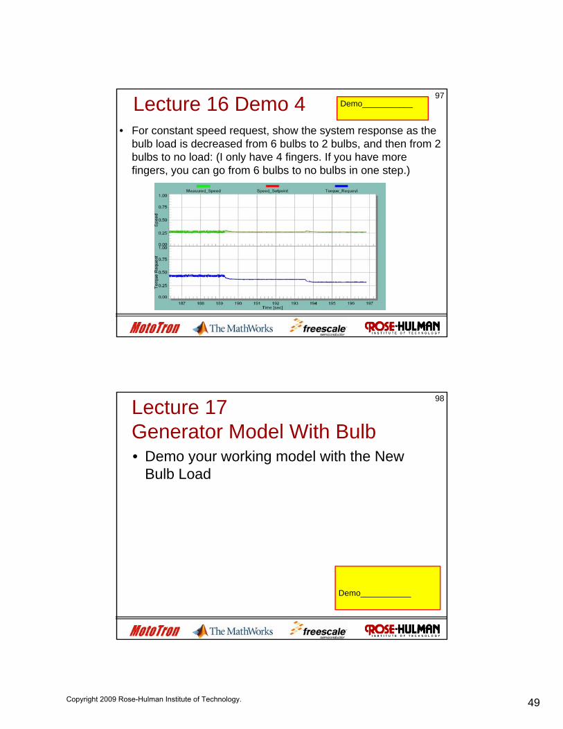
Lecture 16 Demo 4• For constant speed request, show the system response as the

bulb load is decreased from 6 bulbs to 2 bulbs, and then from 2 bulbs to no load: (I only have 4 fingers. If you have more fingers you can go from 6 bulbs to no bulbs in one step )

97Demo___________

fingers, you can go from 6 bulbs to no bulbs in one step.)

Lecture 17 Generator Model With Bulb• Demo your working model with the New

Bulb Load

98

Bulb Load

Demo___________


50

Lecture 18 Demo 1• We notice that we now have overshoot.• Add a second test that verifies that the

overshoot is less than 5%

99

overshoot is less than 5%.• You need to check to see how many tests

pass both the rise time specification and the overshoot specification.

Demo___________

Lecture 18 Exercise 1• Verify summary of results showing that 34

of 35 runs passed the specification.

100

Demo___________


Documents

Lecture 2 Exercise 1awiki.ece.rose-hulman.edu/herniter/images/a/a9/MBSD... · Lecture 3A – Problem1 System Rise Time • We would like to redo our rise time measurement using the