Lecture 2: Firms, Jobs and Policy - Princeton Universityerossi/Macro/Lecture_2_522.pdf · ERH (Princeton University) Lecture 2: Firms, Jobs and Policy Spring 2014 21 / 34. The Model

Lecture 2: Firms, Jobs and PolicyEconomics 522

Esteban Rossi-Hansberg

Princeton University

Spring 2014

ERH (Princeton University ) Lecture 2: Firms, Jobs and Policy Spring 2014 1 / 34

Restuccia and Rogerson (2009)

Assess the quantitative role of resource allocation across productive uses indevelopment

Consider a version of neoclassical growth model with heterogeneous producers

Consider distortions to the prices faced by different producers (idiosyncraticdistortions)

I Credit market imperfections and non-competitive banking systemsI Public enterprisesI Trade restrictionsI Labor market regulationsI Corruption and selective government industrial policy

Resource misallocation can decrease aggregate output and TFP in the rangeof 30 to 50 percent

I A theory of measured TFP


The Model

Infinitely-lived representative household:

∞

∑t=0

βtu(Ct ), 0 < β < 1

Endowments: One unit of productive time each period, K0 > 0 units of thecapital stock, and equal shares of all plants

Budget constraint:

∞

∑t=0

pt (Ct +Kt+1 − (1− δ)Kt ) =∞

∑t=0

pt (rtKt + wtNt + πt − Tt )


Technology

Production unit —a plant:

f (s, k, n) = skαnγ, 0 < γ+ α < 1

Idiosyncratic productivity s constant over time

Exogenous probability of exit λ

Fixed cost of operation cf every period

Entry cost ce and productivity of entrants from cdf H(s)


Policy Distortions

They focus on policies that create idiosyncratic distortions to plant-leveldecisions

Each plant faces its own output tax/subsidy denoted by τ ∈ (−1, 1)Entering plants face draws of s and τ

Given cdf H(s), policy distortions induce a joint distribution cdf G (s, τ)


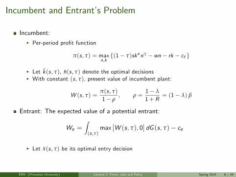
Incumbent and Entrant’s Problem

Incumbent:I Per-period profit function

π(s , τ) = maxn,k{(1− τ)skαnγ − wn− rk − cf }

I Let k̄(s , τ), n̄(s , τ) denote the optimal decisionsI With constant (s , τ), present value of incumbent plant:

W (s , τ) =π(s , τ)1− ρ

, ρ =1− λ

1+ R= (1− λ) β

Entrant: The expected value of a potential entrant:

We =∫(s ,τ)

max [W (s, τ), 0] dG (s, τ)− ce

I Let x̄(s , τ) be its optimal entry decision


Invariant Distribution of Plants

Denote µ(s, τ) the distribution of producing plants this period and E themass of entrants

Next period’s distribution:

µ′(s, τ) = (1− λ)µ(s, τ) + x̄(s, τ)dG (s, τ)E

Let µ̂ be the invariant distribution associated with E = 1:

µ̂(s, τ) =x̄(s, τ)

λdG (s, τ)


Labor Market Clearing

Aggregate labor demand:

N(r ,w) = E∫(s ,τ)

n̄(s, τ)d µ̂(s, τ)

Labor supply inelastic equal to one, entry E satisfies:

E =1∫

(s ,τ) n̄(s, τ)d µ̂(s, τ)


Equilibrium

A steady state competitive equilibrium with entry is w , r , T , µ(s, τ), E , W (s, τ),π(s, τ), We , x̄(s, τ), k̄(s, τ), n̄(s, τ), C , and K such that:

Consumer optimization r = 1/β− (1− δ)

Plant optimization

Free-entry We = 0

Market clearing: labor, capital, output

Government budget balance

T +∫s ,τ

τf (s, k̄, n̄)dµ(s, τ) = 0

Invariant µ

µ(s, τ) = Ex̄(s, τ)

λdG (s, τ)


Calibration

Calibrate undistorted benchmark economy to U.S. data

Model period equal to a year

Parameter Value Targetα 0.3 Capital income shareγ 0.6 Labor income shareβ 0.96 Real rate of returnδ 0.08 Investment to output ratioce 1.0 Normalizationcf 0.0 Benchmark caseλ 0.1 Annual exit rate


Calibration

Key elements: range of s and H(s)

Use mapping from s to n and from H(s) to µ(s) implied by the model

n̄in̄j=

(sisj

) 11−γ−α

µ(s) =x̄(s)

λdH(s)

Number of workers per plant in U.S. Census of Manufactures impliess ∈ [1, 2.43] (given α = 0.3, γ = 0.6, and normalizing lowest s to one)

Micro evidence of TFP suggest range of 1 to 3 across plants within narrowlydefined manufacturing industries


Distribution of Plants by Employment —U.S. Data


Distribution of Plants by Employment —Model vs. Data


Share of Valued Added and Employment


Distribution Statistics of Benchmark Economy

Plant Size by Employment< 10 10 to 499 500 or more

Share of plants 0.51 0.47 0.02Share of output 0.04 0.57 0.39Share of labor 0.04 0.57 0.39Share of capital 0.04 0.57 0.39Average employment 4.2 64.8 1042.0


Aggregate Distortions

An output tax of 0.5 implies relative steady state output(distorted/undistorted) of 0.63

In standard growth model (capital share half the labor share), same tax policyimplies relative steady state output of 0.50.5 = 0.7

Output effect 10 percent larger in model with plant heterogeneity than instandard growth model: accounted for by a fall in measured aggregate TFP

Plant heterogeneity allows another form of aggregate distortions that isempirically relevant: entry cost

I An increase in the cost of entry ce due to government regulation of 50 percentimplies a drop in aggregate measured TFP of 10 percent

I Distortion to the entry cost leave the capital to output ratio unaltered


Idiosyncratic Distortions: Tax/Subsidy Policies

Assume a fraction of plants are taxed and the rest are subsidized

Output tax/subsidy combinations:I Tax packages of 0.1, 0.2, 0.3, 0.4, with subsidies so that the net effect onsteady state capital accumulation is zero

I Lump-sum redistribution to consumers to balance the government budget


Ind. Idiosyncratic Distortions: Tax/Subsidy Policies

τt0.10 0.20 0.30 0.40

Relative Y 0.98 0.95 0.94 0.94Relative TFP 0.98 0.95 0.94 0.94Relative E 1.00 1.00 1.00 1.00Ys/Y 0.80 0.93 0.98 0.99S/Y 0.04 0.06 0.07 0.07τs 0.05 0.07 0.07 0.07


Corr. Idiosyncratic Distortions: Tax/Subsidy Policies

τt0.1 0.2 0.3 0.4

Relative Y 0.87 0.78 0.73 0.72Relative TFP 0.87 0.78 0.73 0.72Relative E 1.00 1.00 1.00 1.00Ys/Y 0.57 0.83 0.95 0.99S/Y 0.20 0.32 0.38 0.40τs 0.35 0.39 0.40 0.40


Sensitivity

Sensitivity of results:I Decreasing returns at the plant level (1− α− γ)I Fixed cost of operation (cf > 0): potential selection of entering plantsI Plant dynamics: potential selection of exiting plants

Capital and human accumulation can amplify these differences


Hopenhayn and Rogerson (1993)

Examine the qualitative and quantitative impact of government policies thatmake it costly for firms to adjust their employment levels

Large volume of job creation and destruction at the level of the individual firm

Important to understand the effects of labor market regulation

Extend Hopenhayn (1992) to a general equilibrium setting

Finding: A tax equal to 1 year’s wages reduces utility by over 2 percentmeasured in terms of consumption

I Important reduction in average labor productivity


The Model

Labor is the only input

Profits are given by

pt f (nt , st )− nt − ptcf − g(nt , nt−1)

where nt denotes employment, wages are normalize to one

st is a firm specific productivity shock, that evolves according to transitionprobabilities F (s, s ′)

I F (s , ·) is the distribution function for next period’s value of the shockI Shock is independent across firms

cf is a fixed operating cost

g captures the presence of adjustment costsI Policy experiments can be represented as changes in gI Firing cost of τ would imply

g (nt , nt−1) = τmax(0, nt−1 − nt )


Timing


Entry and Preferences

Entry cost ceInitial draw s from distribution ν, iid

Continuum of agents uniformly distributed in unit interval with preferences

∞

∑t=1

βt [u (ct )− v (nt )]

where ct > 0 and nt ∈ {0, 1} denote consumption and labor supplyAs in Rogerson (1988) individuals use lotteries and diversify idiosyncratic riskso economy behaves as

∞

∑t=1

βt [u (ct )− aNt ]

where Nt is the fraction of individuals who are employed in period t


Equilibrium

Look at stationary equilibrium so assume constant p

Bellman equation is

W (s, n; p) = maxn′≥0{pf (n′, s)− n′ − pcf − g(n′, n)

+βmax[EsW (s ′, n′; p),−g(0, n′)]}

Optimal decisions N(s, n; p) and X (s, n; p) with X = 1 corresponding to exitand X = 0 stay

Value of entering is

We (p) =∫W (s, 0; p)dv(s).

µ(s, n) denotes the mass of firms with s and n, and M the mass of entrants


AggregatesTotal output is given by

Y (µ,M; p) =∫[f (N(s, n; p), s)− cf ]dµ(s, n) +M

∫f (N(s, 0; p), s)dv(s)

Individual adjustment costs

r(s, n; p) = [1−X (s, n; p)]∫g(N(s ′, n′; p), n′)dF (s, s ′)+X (s, n; p)g(0, n′)

integrate to get R(µ,M, p) the aggregate adjustment costs

Labor demand

Ld (µ,M; p) =∫N(s, n; p)dµ(s, n) +M

∫N(s, 0; p)dv(s)

Profits

Π(µ,M; p) = pY (µ,M; p)− Ld (µ,M; p)− R(µ,M; p)−Mpce

All homogenous of degree one in µ and M


Aggregates

In SS with 1/(1+ r) = β consumer problem is

max u(c)− aNs.t. pc ≤ N +Π+ R

This implies N = LS (p,Π+ R)

A stationary equilibrium consists of an output price p∗ ≥ 0, a mass ofentrants M∗ ≥ 0, and a measure of incumbents ,µ∗, such that

I Ld (µ∗,M∗, p∗) = LS (Π(µ∗,M∗, p∗) + R(µ∗,M∗, p∗))I T (µ∗,M∗, p∗) = µ∗I W e (p∗) ≤ p∗ce with equality if M∗ > 0

Need strict concavity and INADA on f , LS2 < 0, F is continuous F1 < 0 andν has a continuous cdf


Quantitative specification

Benchmark model:

f (n, s) = snθ, 0 ≤ θ ≤ 1g(nt , nt−1) = 0

log(st ) = a+ ρlog(st−1) + εt , where εt ∼ N(0, σ2ε )u (c) = ln (c) and v(n) = An

Persistence ρ < 1 important since it determines how much firms care aboutfiring costs

s exhibits mean reversion


Optimal Rules

For this case n not a state variable so

log nt =1

1− θ(log θ + log p + log st )

X (st , nt , p) = 1 if st ≤ s∗ for some s∗

So employment of surviving firm evolves according to

log nt+1 =1− ρ

1− θ(log θ + log p +

a1− ρ

) + ρ log nt−1 +1

1− θεt (1)


Calibration

Length of period is set to 5 years

Let β = .8 and θ,labor’s share of total revenue, is set to .64

Use (1) to estimate ρ and σε

Fix price p = 1I Choose cf and a to match average of log employment and exit rateI Choose ν to match size distribution in dataI Choose cε so that p = 1


Calibration


DistortionsIntroduce distortions such that

g(nt , nt−1) = τmax(0, nt−1 − nt )

If τ = .2 tax of 1 year of wages


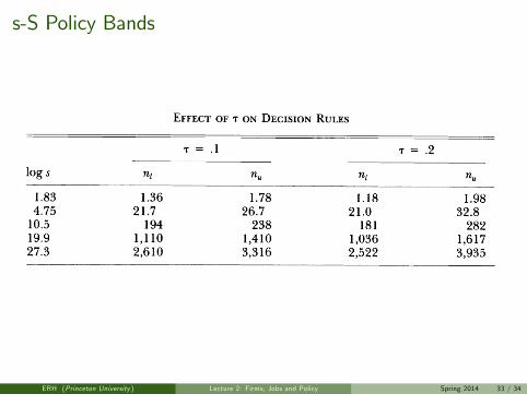
s-S Policy Bands


Deviations from MPL = 1/p


Documents

Lecture 2: Firms, Jobs and Policy - Princeton Universityerossi/Macro/Lecture_2_522.pdf · ERH (Princeton University) Lecture 2: Firms, Jobs and Policy Spring 2014 21 / 34. The Model