1

Lecture 2:Intro/refresher in

Matrix Algebra

Bruce Walsh lecture notesUppsala EQG Courseversion 28 Jan 2012

2

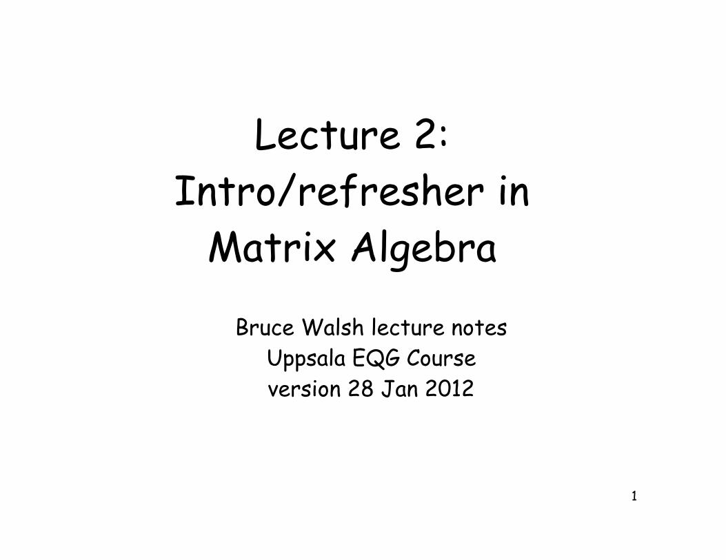
Matrix/linear algebra

• Compact way for treating the algebra ofsystems of linear equations

• Most common statistical methods can bewritten in matrix form– y = X! + e is the general linear model

• OLS solution: ! = (XTX)-1 XT y

– Y = X ! + Z a + e is the general mixed model

3

Topics• Definitions, dimensionality, addition,

subtraction

• Matrix multiplication

• Inverses, solving systems of equations

• Quadratic products and covariances

• The multivariate normal distribution

• Ordinary least squares

• Vector/matrix calculus (taking derivatives)

4

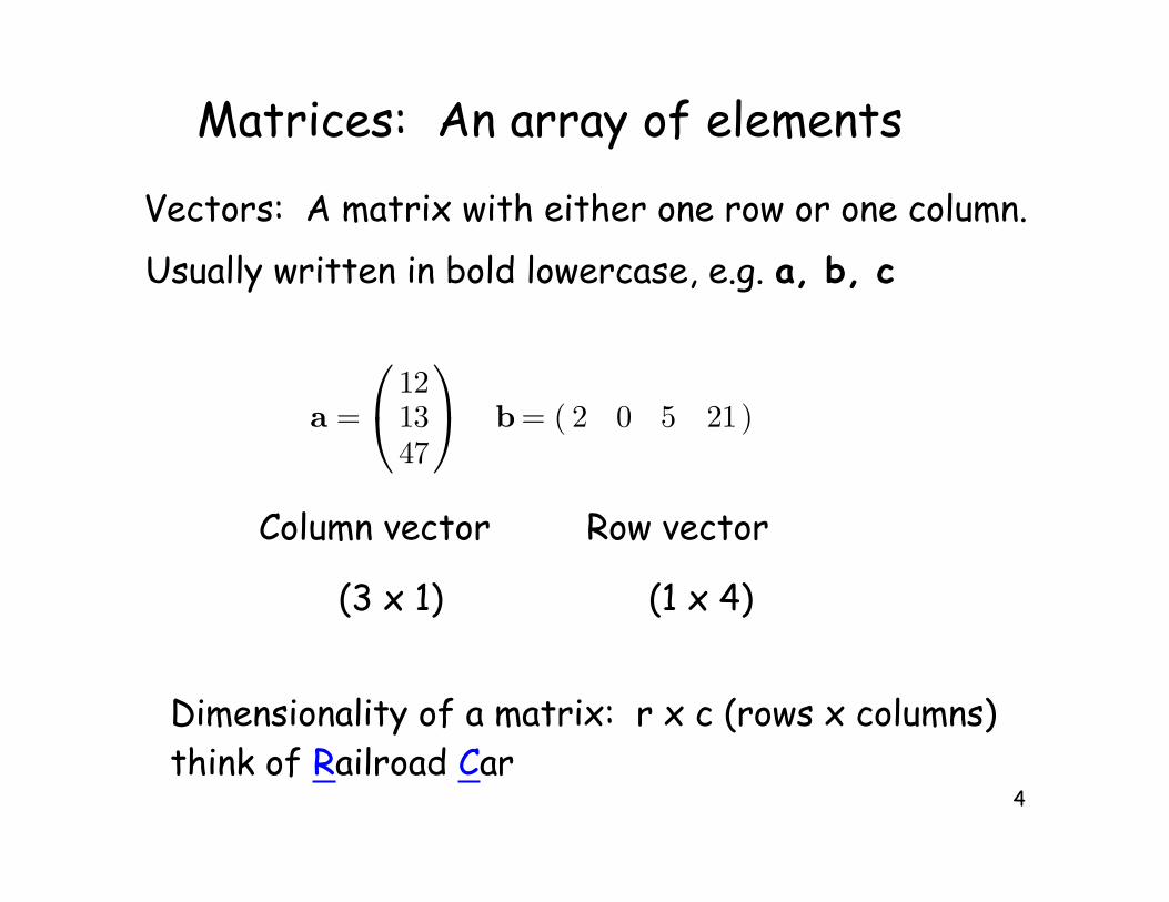
Matrices: An array of elements

Vectors: A matrix with either one row or one column.

Column vector Row vector

(3 x 1) (1 x 4)

Usually written in bold lowercase, e.g. a, b, c

a =

121347

b = ( 2 0 5 21)

Dimensionality of a matrix: r x c (rows x columns)think of Railroad Car

5

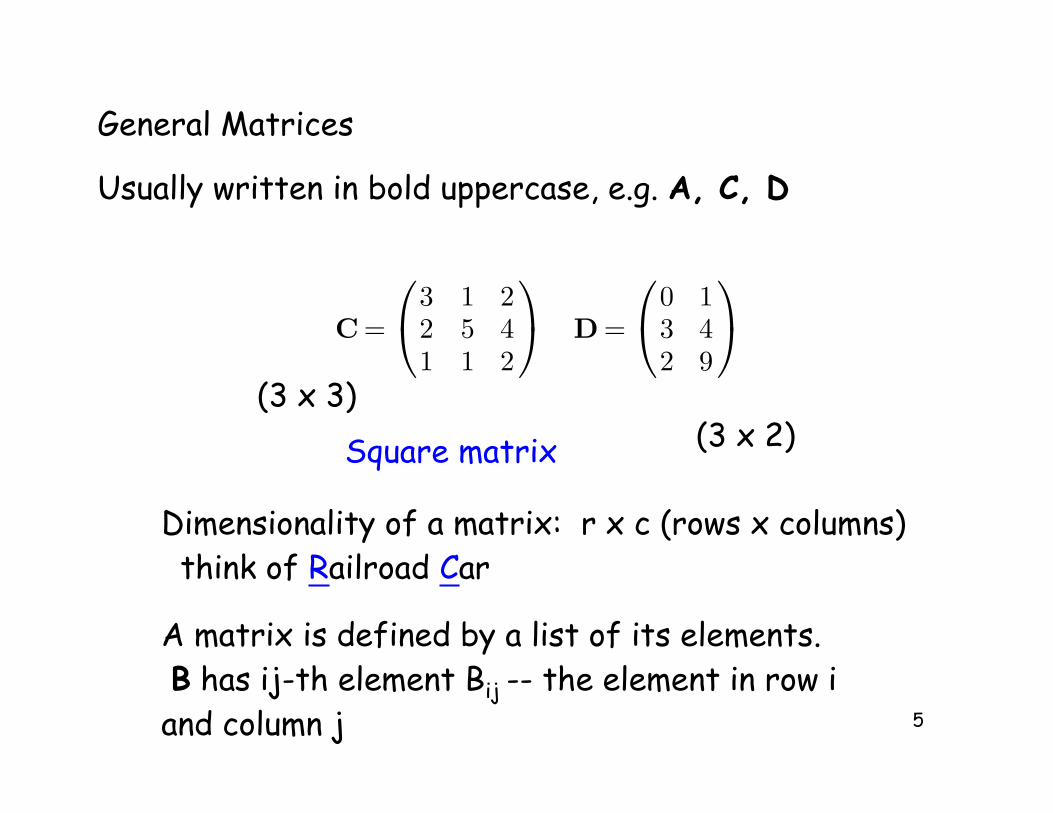
Square matrix

(3 x 3)(3 x 2)

General Matrices

Usually written in bold uppercase, e.g. A, C, D

C =

3 1 22 5 41 1 2

D =

0 13 42 9

Dimensionality of a matrix: r x c (rows x columns) think of Railroad Car

A matrix is defined by a list of its elements. B has ij-th element Bij -- the element in row iand column j

6

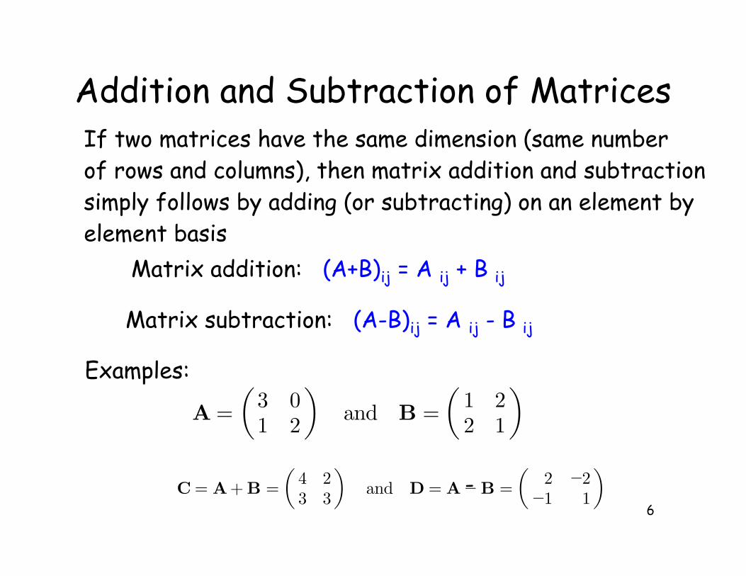
Addition and Subtraction of MatricesIf two matrices have the same dimension (same numberof rows and columns), then matrix addition and subtractionsimply follows by adding (or subtracting) on an element byelement basis

Matrix addition: (A+B)ij = A ij + B ij

Matrix subtraction: (A-B)ij = A ij - B ij

Examples:

A =(

3 01 2

)and B =

(1 22 1

)

C = A+ B =(

4 23 3

)and D = A−B =

(2 −2−1 1

)-

7

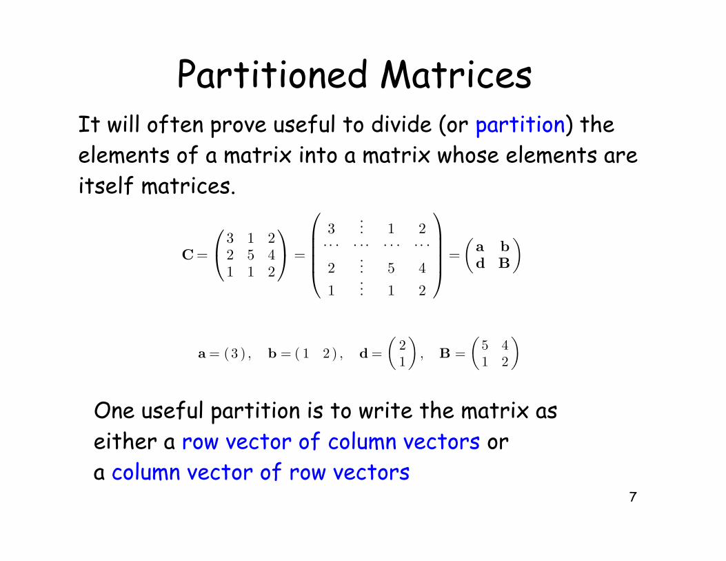
Partitioned MatricesIt will often prove useful to divide (or partition) the elements of a matrix into a matrix whose elements areitself matrices.

C =

3 1 22 5 41 1 2

=

3... 1 2

· · · · · · · · · · · ·2

... 5 41

... 1 2

=(

a bd B

)

a = (3 ) , b = ( 1 2 ) , d =(

21

), B =

(5 41 2

)

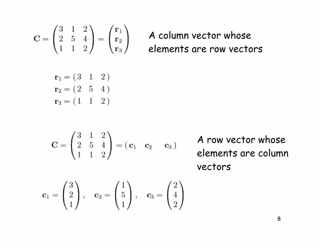
One useful partition is to write the matrix aseither a row vector of column vectors ora column vector of row vectors

8

A row vector whose elements are column vectors

A column vector whose elements are row vectors

9

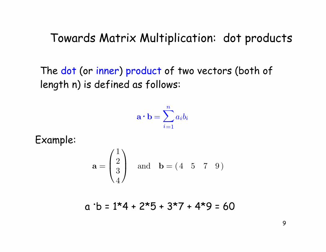
Towards Matrix Multiplication: dot products

The dot (or inner) product of two vectors (both oflength n) is defined as follows:

Example:

a .b = 1*4 + 2*5 + 3*7 + 4*9 = 60

a · b =n∑

i=1

aibi.

a =

1234

and b = (4 5 7 9 )

10

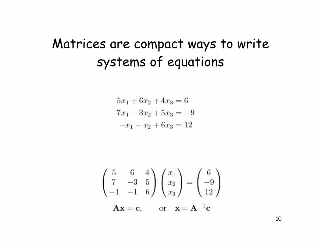
Matrices are compact ways to writesystems of equations

11

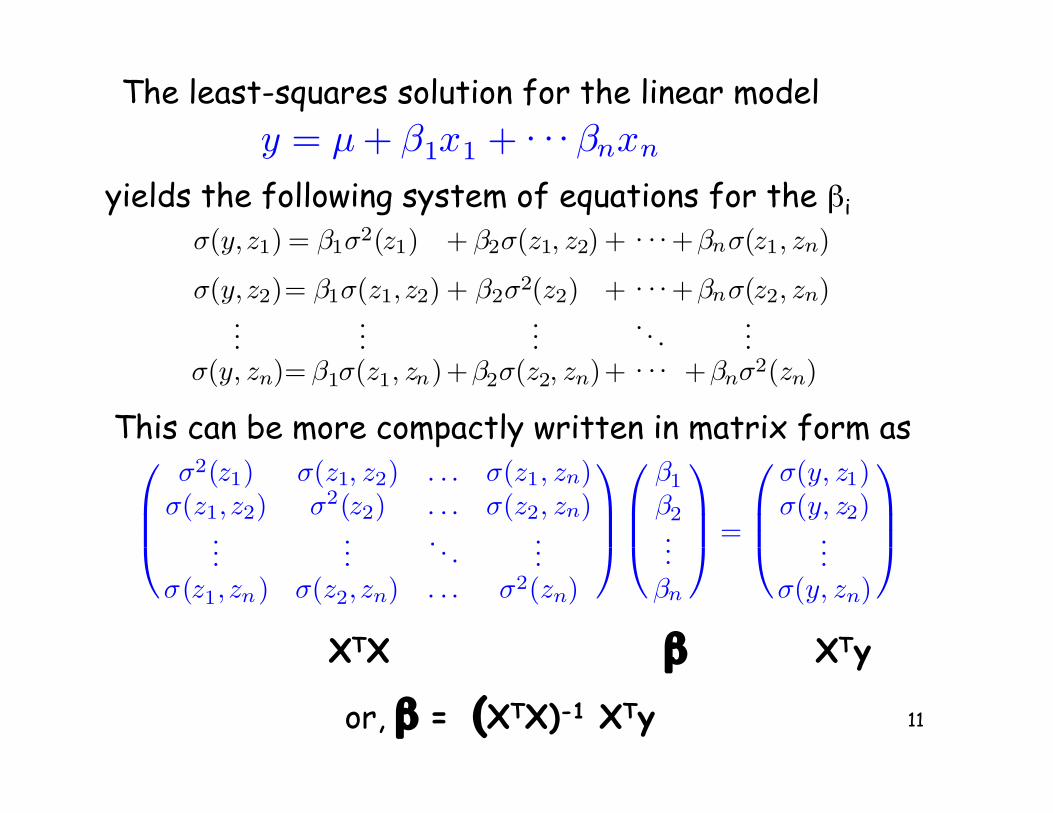
y = µ + β1x1 + · · · βnxn

The least-squares solution for the linear model

yields the following system of equations for the !i

σ(y,z1) = β1σ2(z1) + β2σ(z1, z2) + · · · +βnσ(z1, zn)

σ(y,z2)= β1σ(z1, z2) + β2σ2(z2) + · · · +βnσ(z2, zn)...

......

. . ....

σ(y, zn)= β1σ(z1, zn)+β2σ(z2, zn)+ · · · +βnσ2(zn)

This can be more compactly written in matrix form as

σ2(z1) σ(z1, z2) . . . σ(z1, zn)σ(z1, z2) σ2(z2) . . . σ(z2, zn)

......

. . ....

σ(z1, zn) σ(z2, zn) . . . σ2(zn)

β1

β2...

βn

=

σ(y, z1)σ(y, z2)

...σ(y, zn)

XTX XTy!

or, ! = (XTX)-1 XTy

12

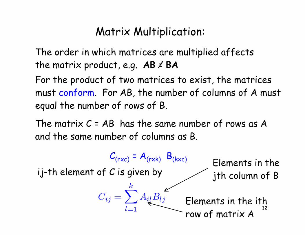
Matrix Multiplication:

The order in which matrices are multiplied affectsthe matrix product, e.g. AB = BA

For the product of two matrices to exist, the matricesmust conform. For AB, the number of columns of A mustequal the number of rows of B.

The matrix C = AB has the same number of rows as Aand the same number of columns as B.

C(rxc) = A(rxk) B(kxc)

ij-th element of C is given by

Cij =k∑

l=1

AilBlj Elements in the ithrow of matrix A

Elements in thejth column of B

13

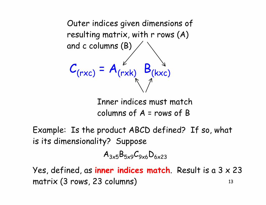
C(rxc) = A(rxk) B(kxc)

Inner indices must matchcolumns of A = rows of B

Outer indices given dimensions ofresulting matrix, with r rows (A)and c columns (B)

Example: Is the product ABCD defined? If so, whatis its dimensionality? Suppose

A3x5B5x9C9x6D6x23

Yes, defined, as inner indices match. Result is a 3 x 23matrix (3 rows, 23 columns)

14

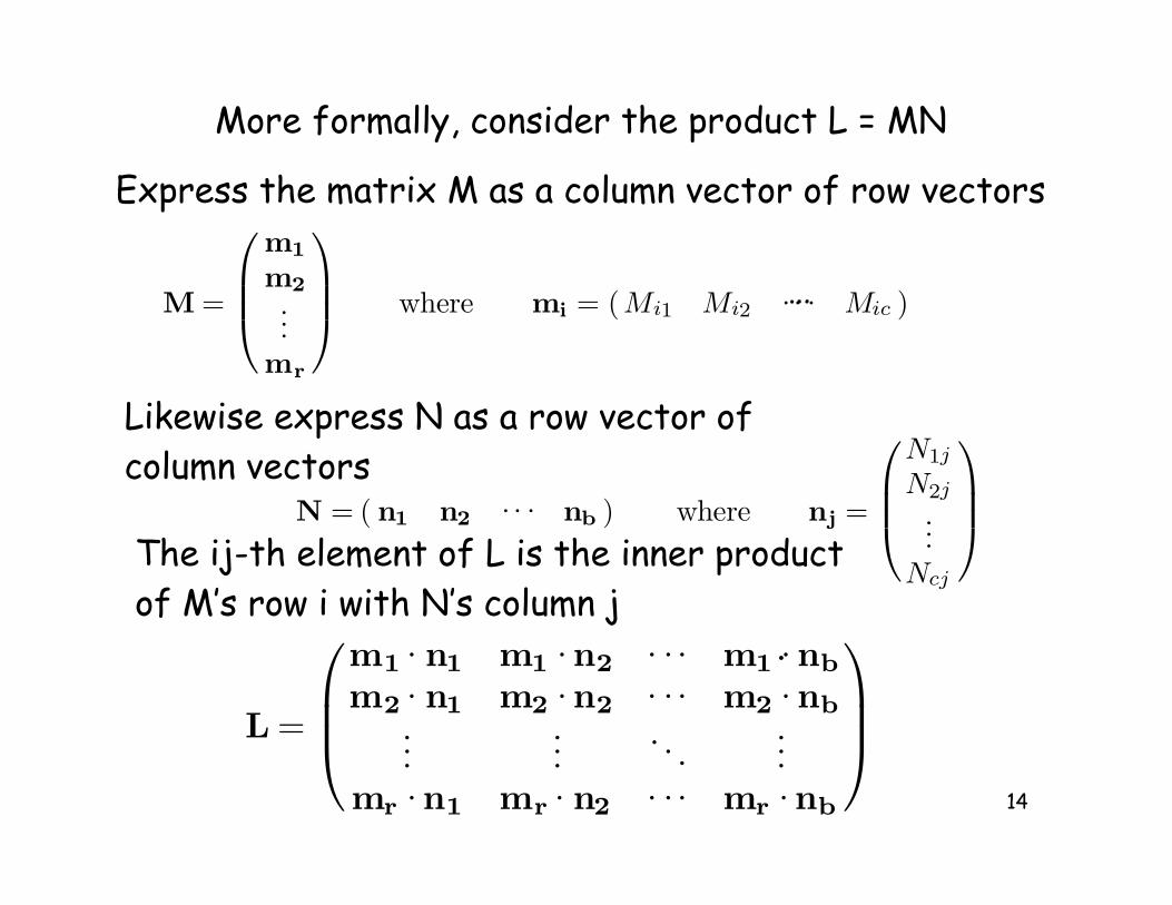
More formally, consider the product L = MN

M =

m1

m2...

mr

where mi = (Mi1 Mi2 · · · Mic )…

Express the matrix M as a column vector of row vectors

N = ( n1 n2 · · · nb ) where nj =

N1j

N2j

...Ncj

Likewise express N as a row vector ofcolumn vectors

The ij-th element of L is the inner productof M’s row i with N’s column j

L =

m1 · n1 m1 · n2 · · · m1 · nb

m2 · n1 m2 · n2 · · · m2 · nb...

.... . .

...mr · n1 mr · n2 · · · mr · nb

.

15

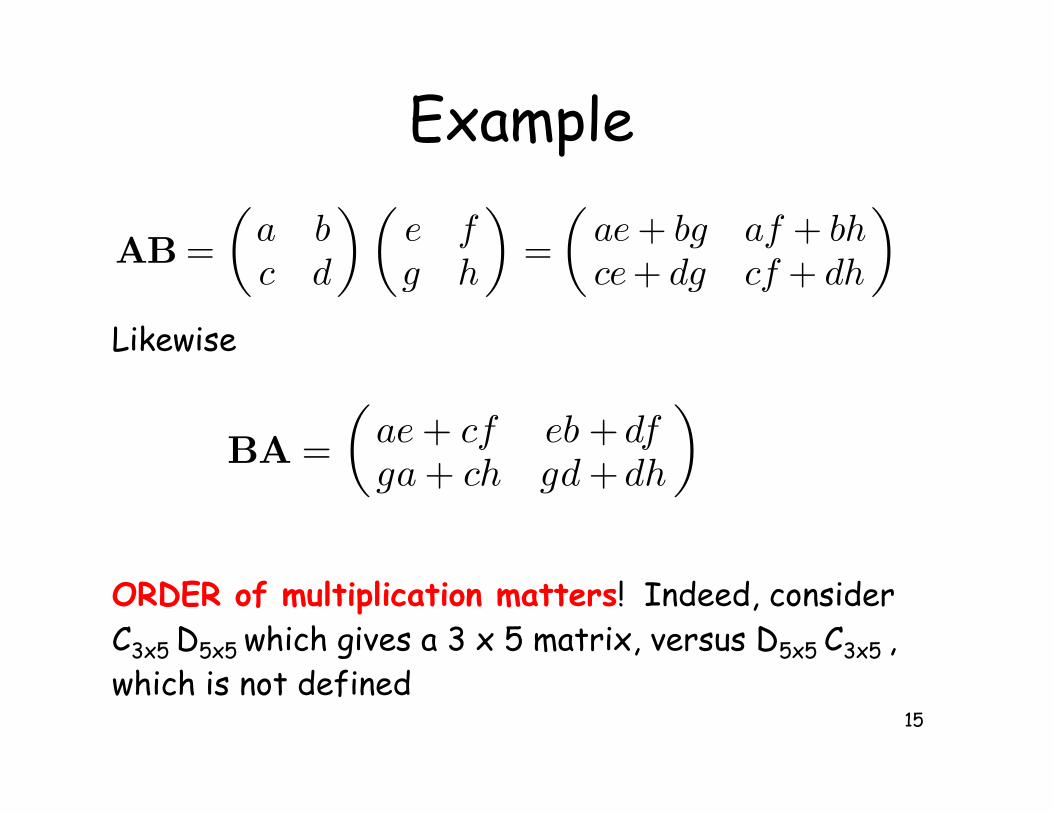
Example

AB =(

a bc d

) (e fg h

)=

(ae + bg af + bhce+ dg cf + dh

)

BA =(

ae + cf eb +dfga + ch gd +dh

)Likewise

ORDER of multiplication matters! Indeed, considerC3x5 D5x5 which gives a 3 x 5 matrix, versus D5x5 C3x5 , which is not defined

16

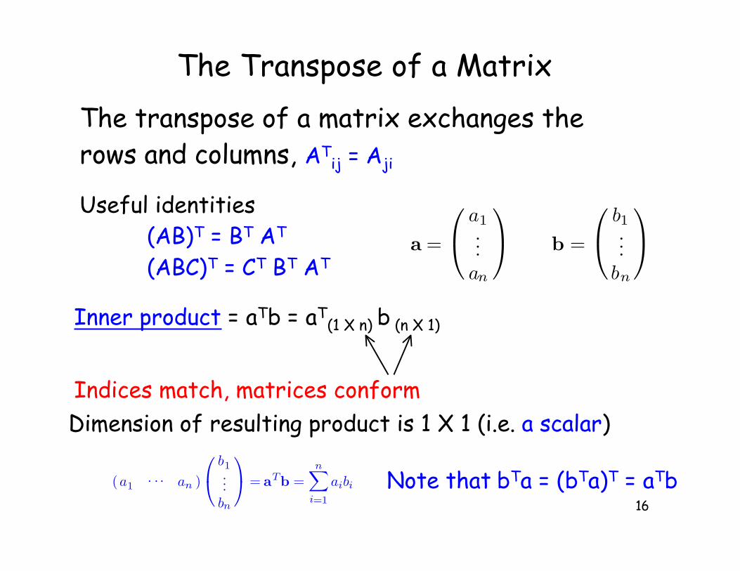
The Transpose of a Matrix

The transpose of a matrix exchanges the rows and columns, AT

ij = Aji

Useful identities(AB)T = BT AT

(ABC)T = CT BT AT

Inner product = aTb = aT(1 X n) b

(n X 1)

Indices match, matrices conform

Dimension of resulting product is 1 X 1 (i.e. a scalar)

a =

a1...an

b =

b1...

bn

(a1 · · · an )

b1...

bn

= aTb =

n∑

i=1

aibi Note that bTa = (bTa)T = aTb

17

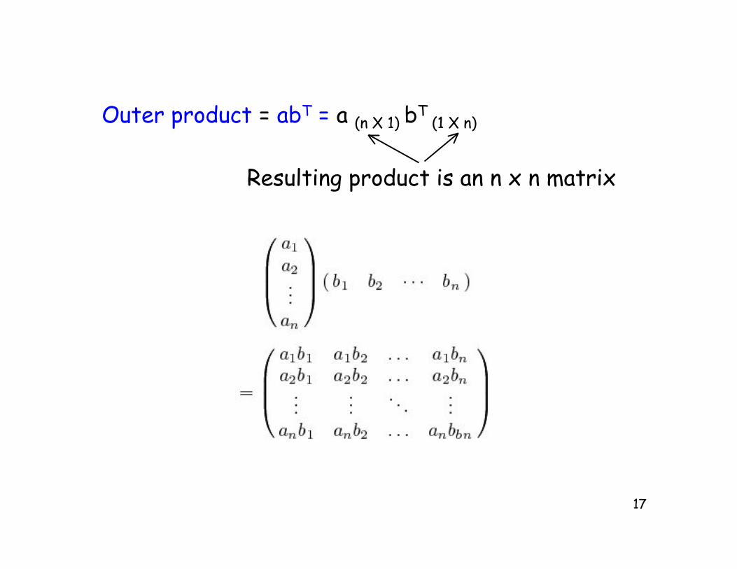
Outer product = abT = a (n X 1) bT (1 X n)

Resulting product is an n x n matrix

18

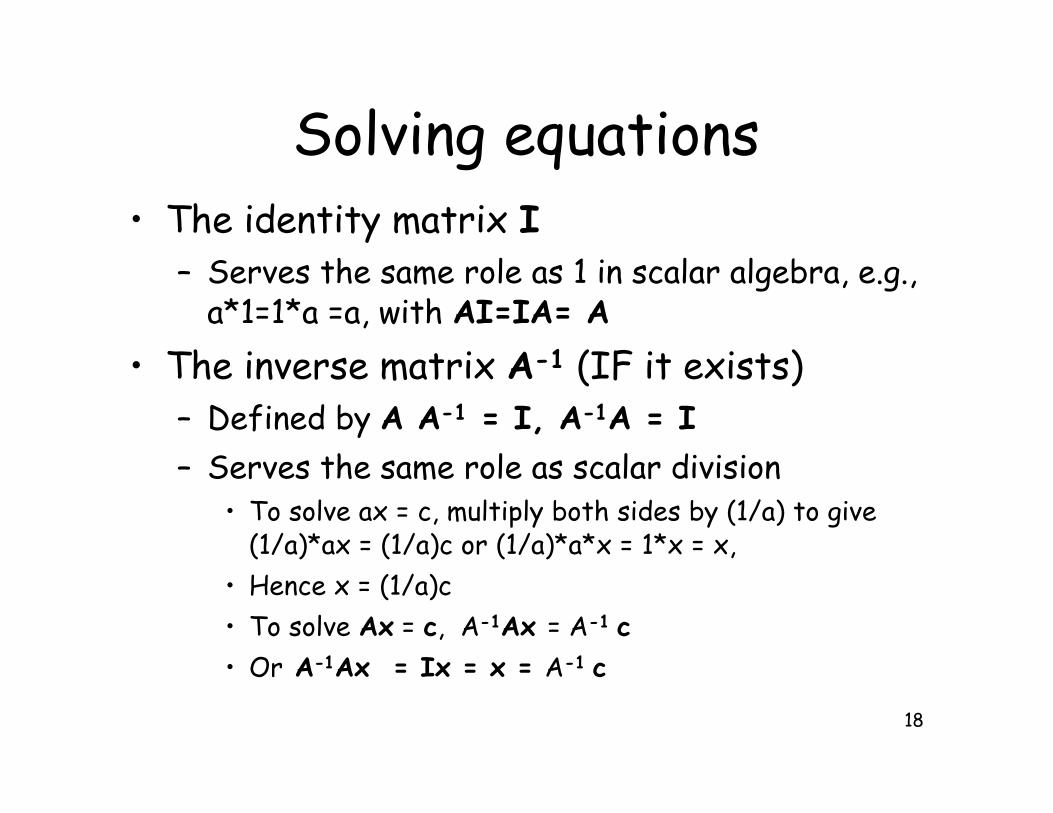
Solving equations• The identity matrix I

– Serves the same role as 1 in scalar algebra, e.g.,a*1=1*a =a, with AI=IA= A

• The inverse matrix A-1 (IF it exists)– Defined by A A-1 = I, A-1A = I

– Serves the same role as scalar division• To solve ax = c, multiply both sides by (1/a) to give

(1/a)*ax = (1/a)c or (1/a)*a*x = 1*x = x,

• Hence x = (1/a)c

• To solve Ax = c, A-1Ax = A-1 c

• Or A-1Ax = Ix = x = A-1 c

19

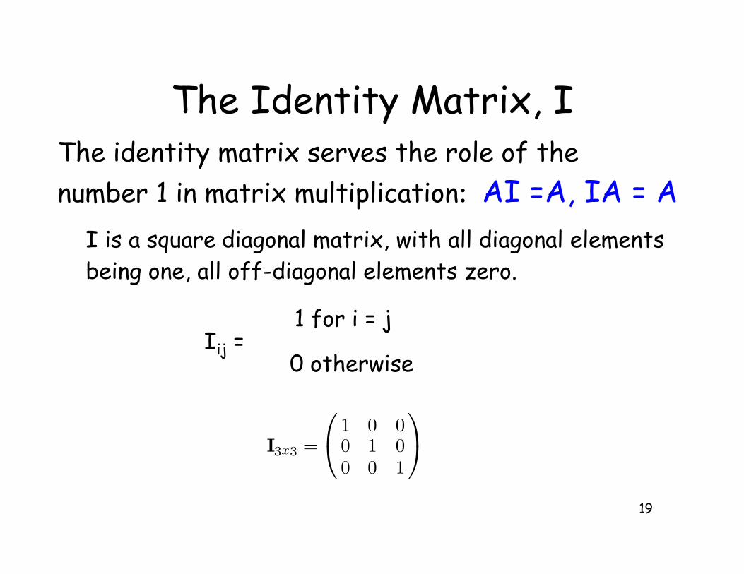
The Identity Matrix, IThe identity matrix serves the role of the

number 1 in matrix multiplication: AI =A, IA = A

I is a square diagonal matrix, with all diagonal elementsbeing one, all off-diagonal elements zero.

Iij = 1 for i = j

0 otherwise

I3x3 =

1 0 00 1 00 0 1

20

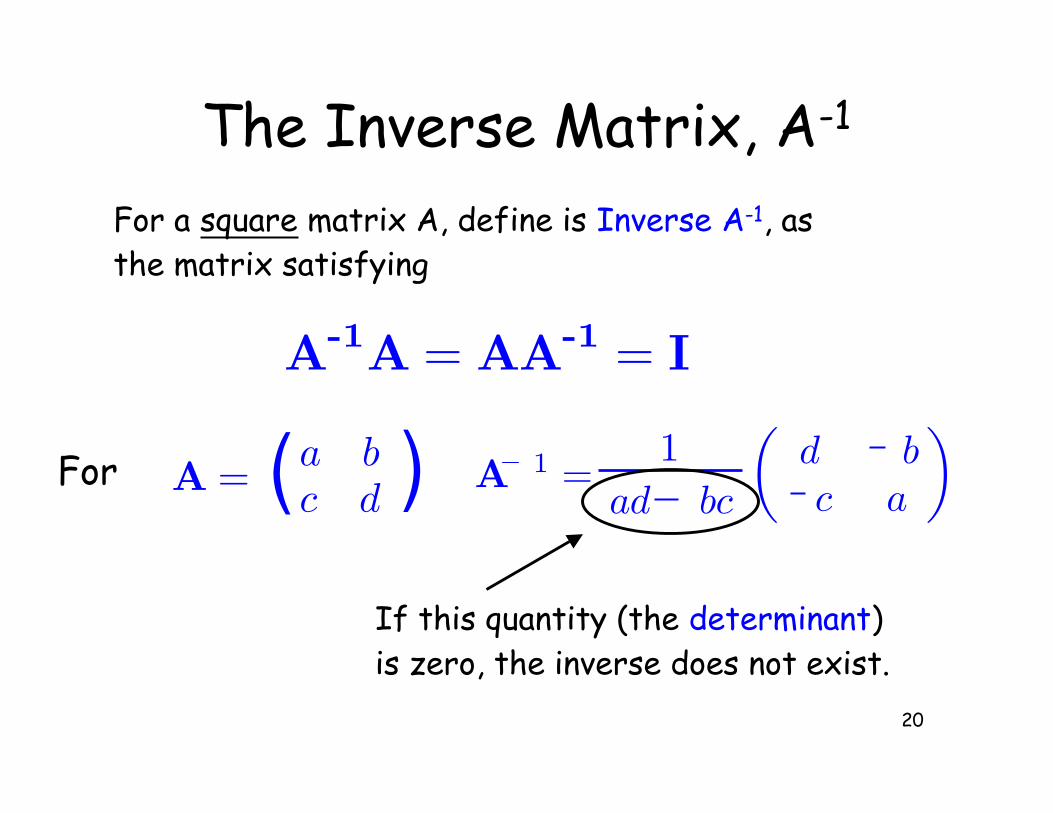
The Inverse Matrix, A-1

)(A = a bc d

For

For a square matrix A, define is Inverse A-1, asthe matrix satisfying

A-1A = AA-1 = I

A 1 =1

ad bc

(d bc a

)

If this quantity (the determinant)is zero, the inverse does not exist.

21

If det(A) is not zero, A-1 exists and A is said to benon-singular. If det(A) = 0, A is singular, and nounique inverse exists (generalized inverses do)

Generalized inverses, and their uses in solving systemsof equations, are discussed in Appendix 3 of Lynch & Walsh

A- is the typical notation to denote the G-inverse of amatrix

When a G-inverse is used, provided the system is consistent, then some of the variables have a familyof solutions (e.g., x1 =2, but x2 + x3 = 6)

22

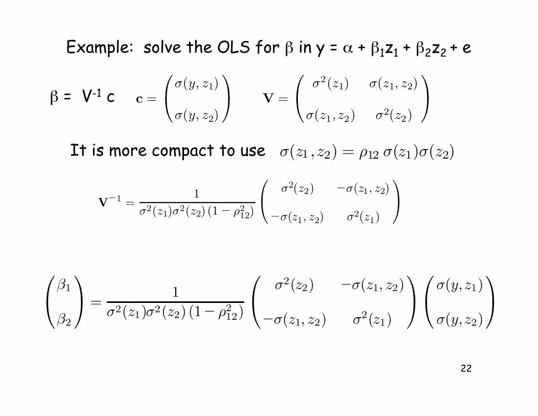
Example: solve the OLS for ! in y = " + !1z1 + !2z2 + e

c =

σ(y, z1)

σ(y, z2)

V =

σ2(z1) σ(z1, z2)

σ(z1, z2) σ2(z2)

! = V-1 c

σ(z1 ,z2) = ρ12 σ(z1)σ(z2)It is more compact to use

V−1 =1

σ2(z1)σ2(z2) (1− ρ212)

σ2(z2) −σ(z1, z2)

−σ(z1, z2) σ2(z1)

β1

β2

=1

σ2(z1)σ2(z2) (1− ρ212)

σ2(z2) −σ(z1, z2)

−σ(z1, z2) σ2(z1)

σ(y,z1)

σ(y,z2)

23

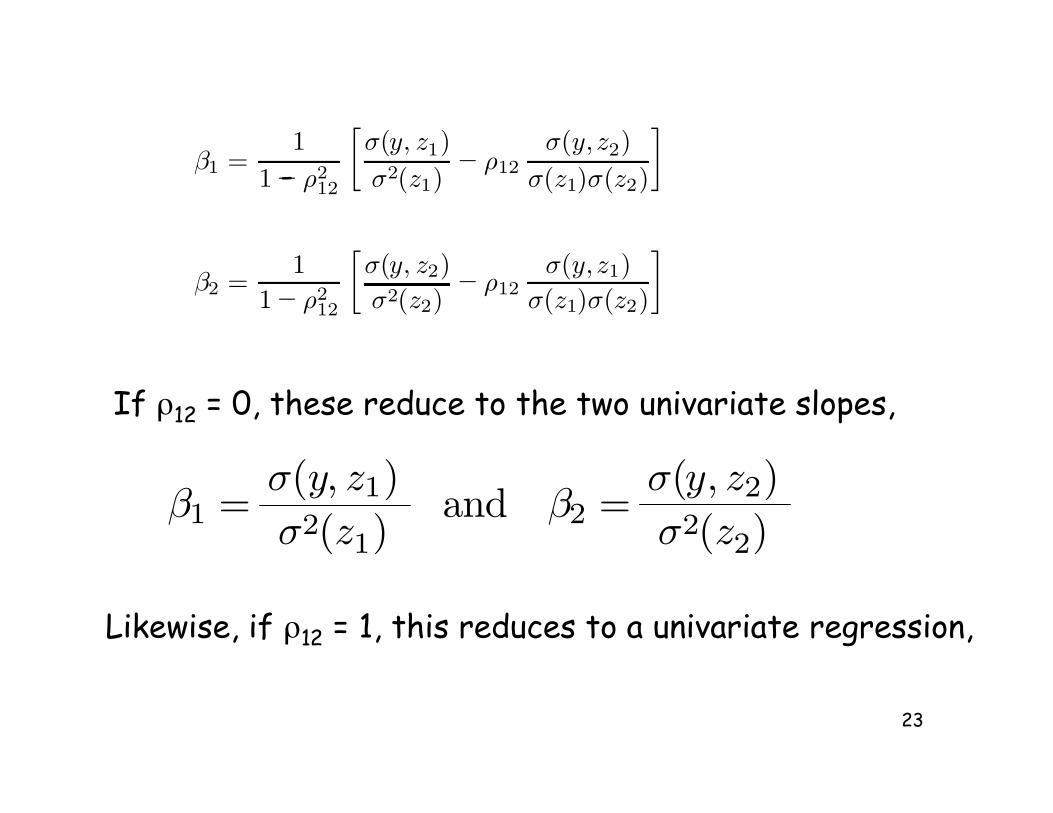
If #12 = 0, these reduce to the two univariate slopes,

β1 =σ(y, z1)σ2(z1)

and β2 =σ(y, z2)σ2(z2)

β1 =1

1− ρ212

[σ(y, z1)σ2(z1)

− ρ12σ(y,z2)

σ(z1)σ(z2)

]

β2 =1

1− ρ212

[σ(y, z2)σ2(z2)

− ρ12σ(y,z1)

σ(z1)σ(z2)

]

-

Likewise, if #12 = 1, this reduces to a univariate regression,

24

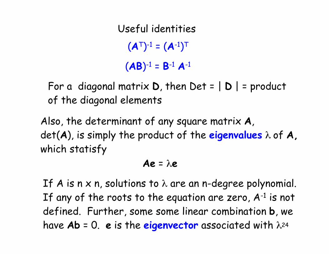
Useful identities

(AB)-1 = B-1 A-1

(AT)-1 = (A-1)T

Also, the determinant of any square matrix A, det(A), is simply the product of the eigenvalues $ of A,

which statisfy

Ae = $e

If A is n x n, solutions to $ are an n-degree polynomial.If any of the roots to the equation are zero, A-1 is notdefined. Further, some some linear combination b, wehave Ab = 0. e is the eigenvector associated with $

For a diagonal matrix D, then Det = | D | = productof the diagonal elements

25

Variance-Covariance matrix

• A very important square matrix is thevariance-covariance matrix V associatedwith a vector x of random variables.

• Vij = Cov(xi,xj), so that the i-th diagonalelement of V is the variance of xi, and off-diagonal elements are covariances

• V is a symmetric, square matrix

26

The traceThe trace, tr(A) or trace(A), of a square matrixA is simply the sum of its diagonal elements

The importance of the trace is that it equals

the sum of the eigenvalues of A, tr(A) = % $i

For a covariance matrix V, tr(V) measures thetotal amount of variation in the variables

$i / tr(V) is the fraction of the total variation in x contained in the linear combination ei

Tx, whereei, the i-th principal component of V is also thei-th eigenvector of V (Vei = $i ei)

27

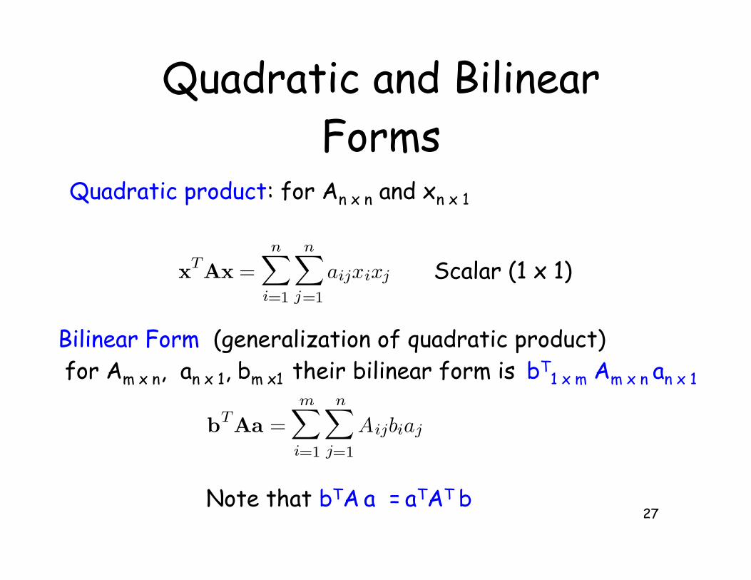
Quadratic and BilinearForms

Quadratic product: for An x n and xn x 1

xTAx =n∑

i=1

n∑

j=1

aijxixj Scalar (1 x 1)

Bilinear Form (generalization of quadratic product) for Am x n, an x 1, bm x1 their bilinear form is bT

1 x m Am x n an x 1

Note that bTA a = aTAT b

bTAa =m∑

i=1

n∑

j=1

Aijbiaj

28

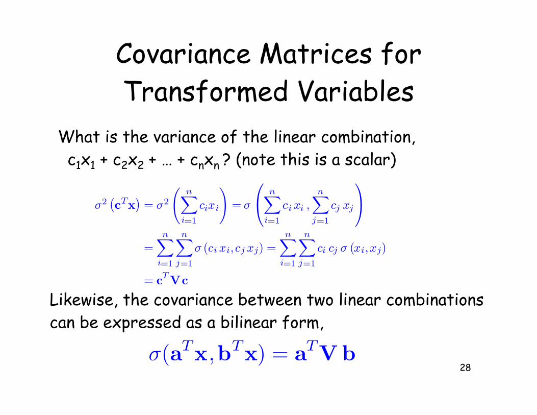
Covariance Matrices forTransformed Variables

σ2(cTx

)= σ2

(n∑

i=1

cixi

)= σ

n∑

i=1

ci xi ,n∑

j=1

cj xj

=n∑

i=1

n∑

j=1

σ (ci xi, cj xj) =n∑

i=1

n∑

j=1

ci cj σ (xi,xj)

= cTVc

What is the variance of the linear combination, c1x1 + c2x2 + … + cnxn ? (note this is a scalar)

Likewise, the covariance between two linear combinationscan be expressed as a bilinear form,

σ(aTx,bTx) = aTVb

29

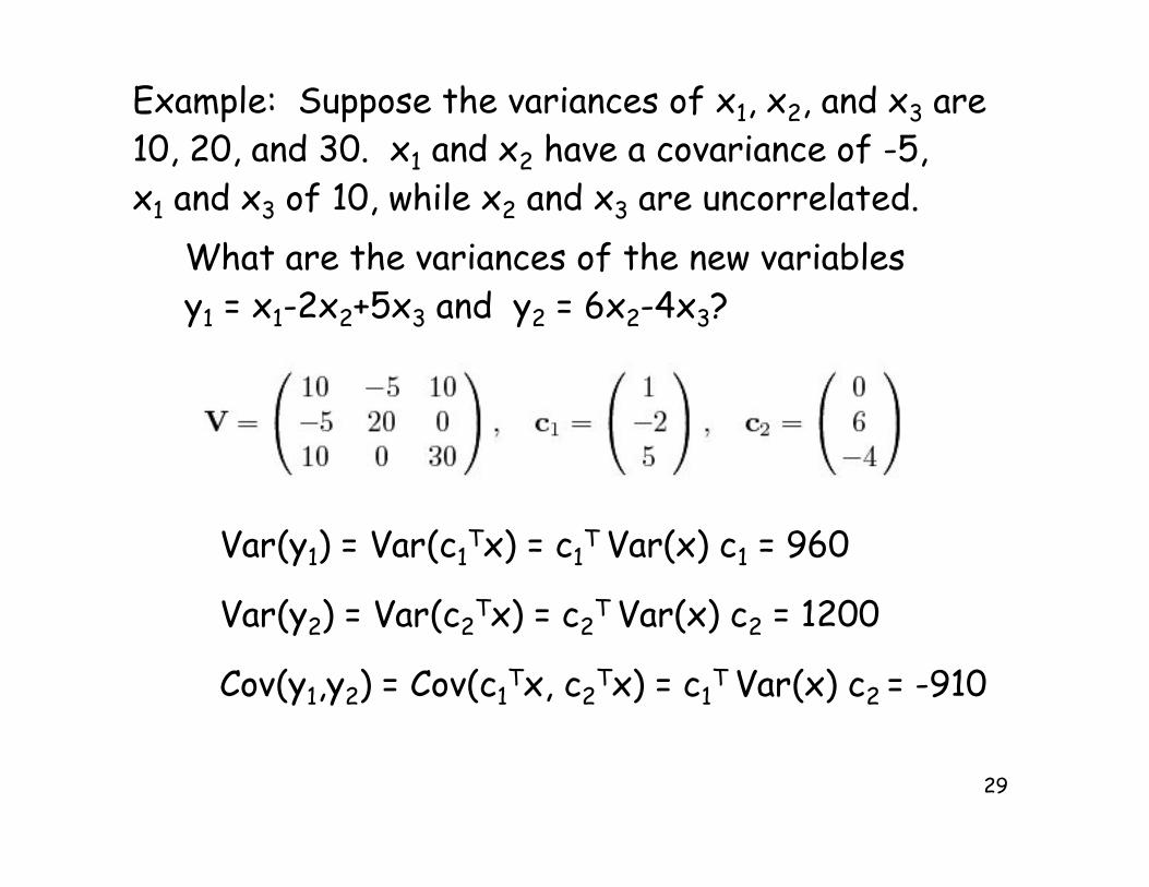
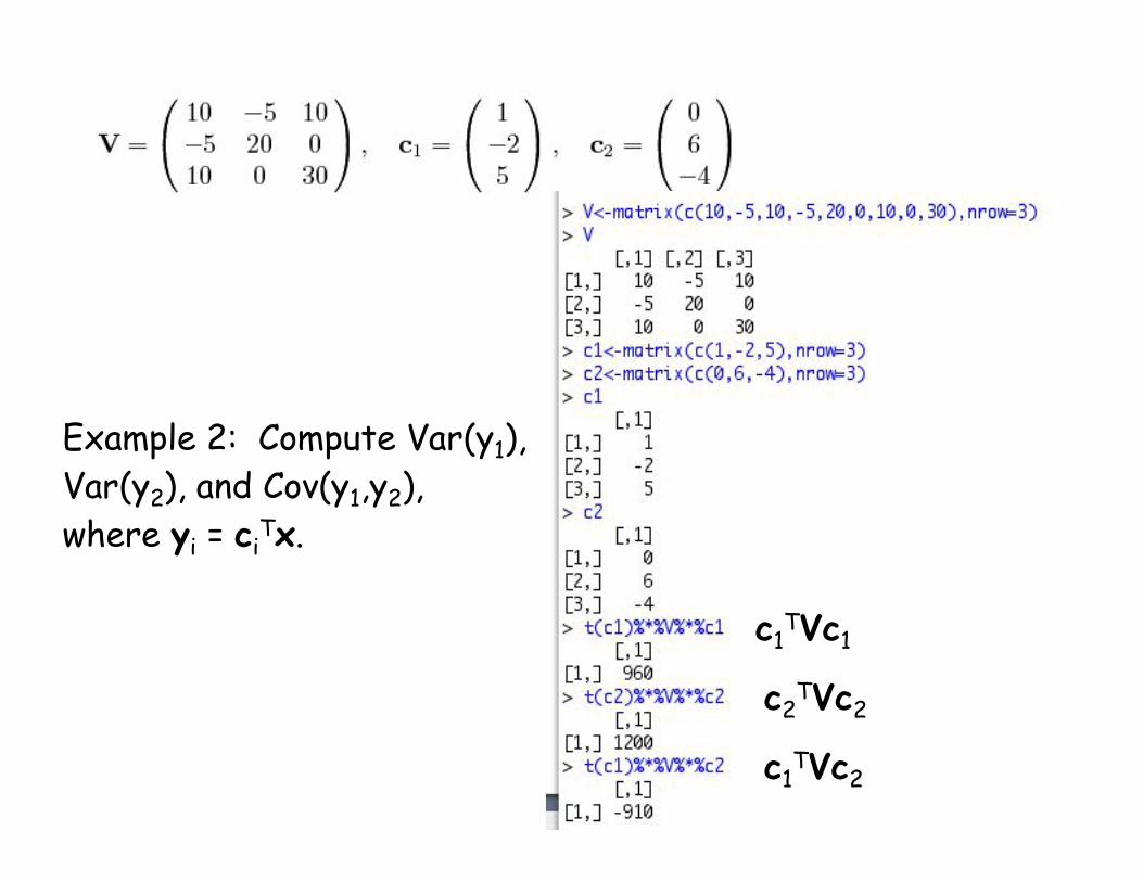
Example: Suppose the variances of x1, x2, and x3 are10, 20, and 30. x1 and x2 have a covariance of -5,x1 and x3 of 10, while x2 and x3 are uncorrelated.

What are the variances of the new variablesy1 = x1-2x2+5x3 and y2 = 6x2-4x3?

Var(y1) = Var(c1Tx) = c1

T Var(x) c1 = 960

Var(y2) = Var(c2Tx) = c2

T Var(x) c2 = 1200

Cov(y1,y2) = Cov(c1Tx, c2

Tx) = c1T Var(x) c2 = -910

30

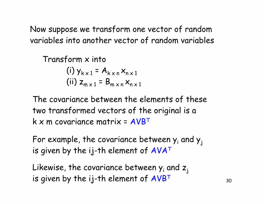
Now suppose we transform one vector of randomvariables into another vector of random variables

Transform x into (i) yk x 1 = Ak x n xn x 1

(ii) zm x 1 = Bm x n xn x 1

The covariance between the elements of thesetwo transformed vectors of the original is ak x m covariance matrix = AVBT

For example, the covariance between yi and yj

is given by the ij-th element of AVAT

Likewise, the covariance between yi and zj

is given by the ij-th element of AVBT

31

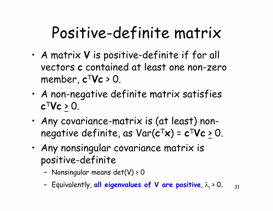
Positive-definite matrix• A matrix V is positive-definite if for all

vectors c contained at least one non-zeromember, cTVc > 0.

• A non-negative definite matrix satisfiescTVc > 0.

• Any covariance-matrix is (at least) non-negative definite, as Var(cTx) = cTVc > 0.

• Any nonsingular covariance matrix ispositive-definite– Nonsingular means det(V) > 0

– Equivalently, all eigenvalues of V are positive, $i > 0.

32

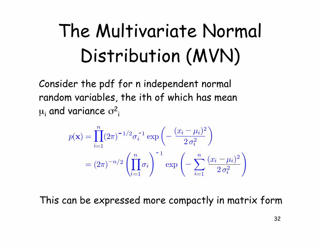
The Multivariate NormalDistribution (MVN)

Consider the pdf for n independent normalrandom variables, the ith of which has meanµi and variance &2

i

This can be expressed more compactly in matrix form

p(x) =n∏

i=1

(2π) 1/2σ 1i exp

(− (xi− µi)2

2σ2i

)

= (2π)−n/2

(n∏

i=1

σi

) 1

exp

(−

n∑

i=1

(xi −µi)2

2σ2i

)

- -

-

33

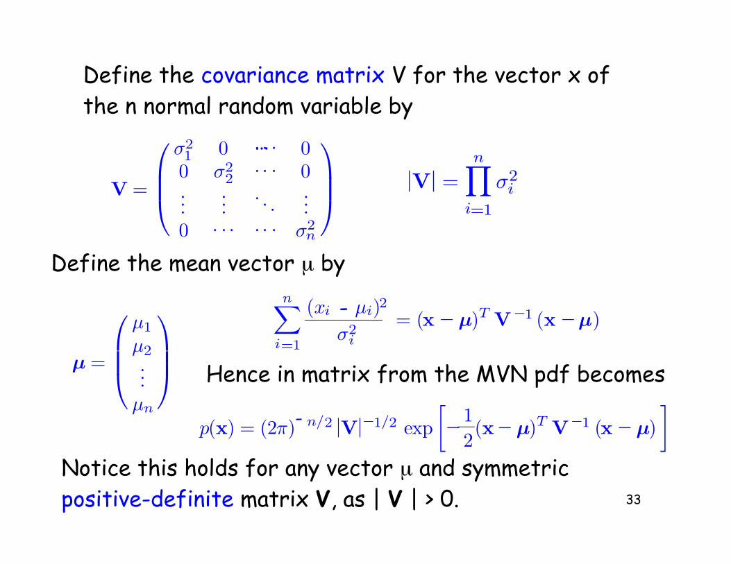
Define the covariance matrix V for the vector x of the n normal random variable by

Define the mean vector µ by

Hence in matrix from the MVN pdf becomes

Notice this holds for any vector µ and symmetricpositive-definite matrix V, as | V | > 0.

|V| =n∏

i=1

σ2iV =

σ21 0 · · · 00 σ2

2 · · · 0...

.... . .

...0 · · · · · · σ2

n

…

n-∑

i=1

(xi µi)2

σ2i

= (x −µ)T V−1 (x −µ)

µ =

µ1

µ2...

µn

p(x) = (2π) n/2 |V|−1/2 exp[−1

2(x−µ)T V−1 (x −µ)

]-

34

The multivariate normal

• Just as a univariate normal is definedby its mean and spread, a multivariatenormal is defined by its mean vectorµ (also called the centroid) andvariance-covariance matrix V

35

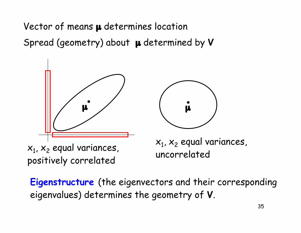
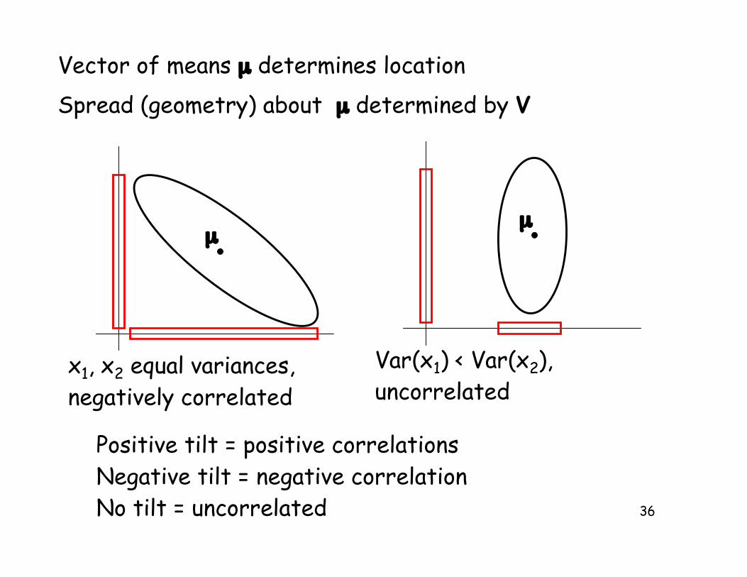
Vector of means µ determines location

µ

Spread (geometry) about µ determined by V

µ

x1, x2 equal variances,positively correlated

x1, x2 equal variances,uncorrelated

Eigenstructure (the eigenvectors and their correspondingeigenvalues) determines the geometry of V.

36

Vector of means µ determines location

µ

Spread (geometry) about µ determined by V

x1, x2 equal variances,negatively correlated

µ

Var(x1) < Var(x2), uncorrelated

Positive tilt = positive correlationsNegative tilt = negative correlationNo tilt = uncorrelated

37

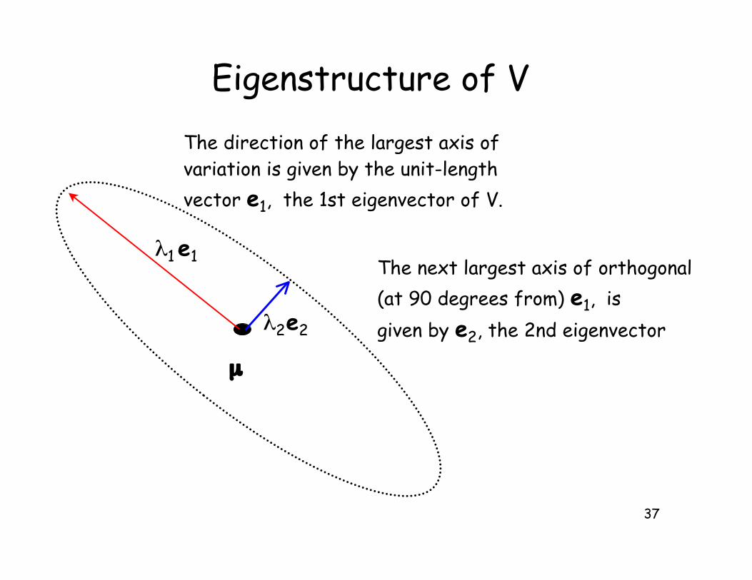
Eigenstructure of V

µ

e1$1

e2$2

The direction of the largest axis of variation is given by the unit-length

vector e1, the 1st eigenvector of V.

The next largest axis of orthogonal

(at 90 degrees from) e1, is

given by e2, the 2nd eigenvector

38

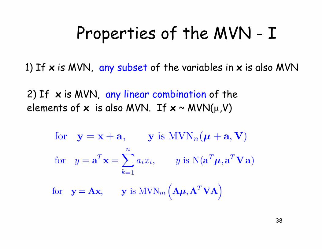
Properties of the MVN - I

1) If x is MVN, any subset of the variables in x is also MVN

2) If x is MVN, any linear combination of the elements of x is also MVN. If x ~ MVN(µ,V)

for y = x + a, y is MVNn(µ + a, V)

for y = aT x =n∑

k=1

aixi, y is N(aTµ,aT Va)

for y = Ax, y is MVNm

(Aµ,AT VA

)

39

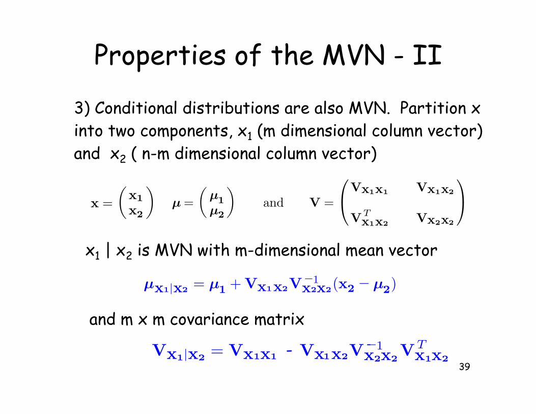
Properties of the MVN - II

3) Conditional distributions are also MVN. Partition xinto two components, x1 (m dimensional column vector)and x2 ( n-m dimensional column vector)

x1 | x2 is MVN with m-dimensional mean vector

and m x m covariance matrix

x =(

x1

x2

)µ =

(µ1µ2

)and V =

Vx1x1 Vx1x2

VTx1x2

Vx2x2

µx1|x2 = µ1 + Vx1x2V−1x2x2(x2 −µ2)

--Vx1|x2= Vx1x1 Vx1x2V

−1x2x2VT

x1x2

40

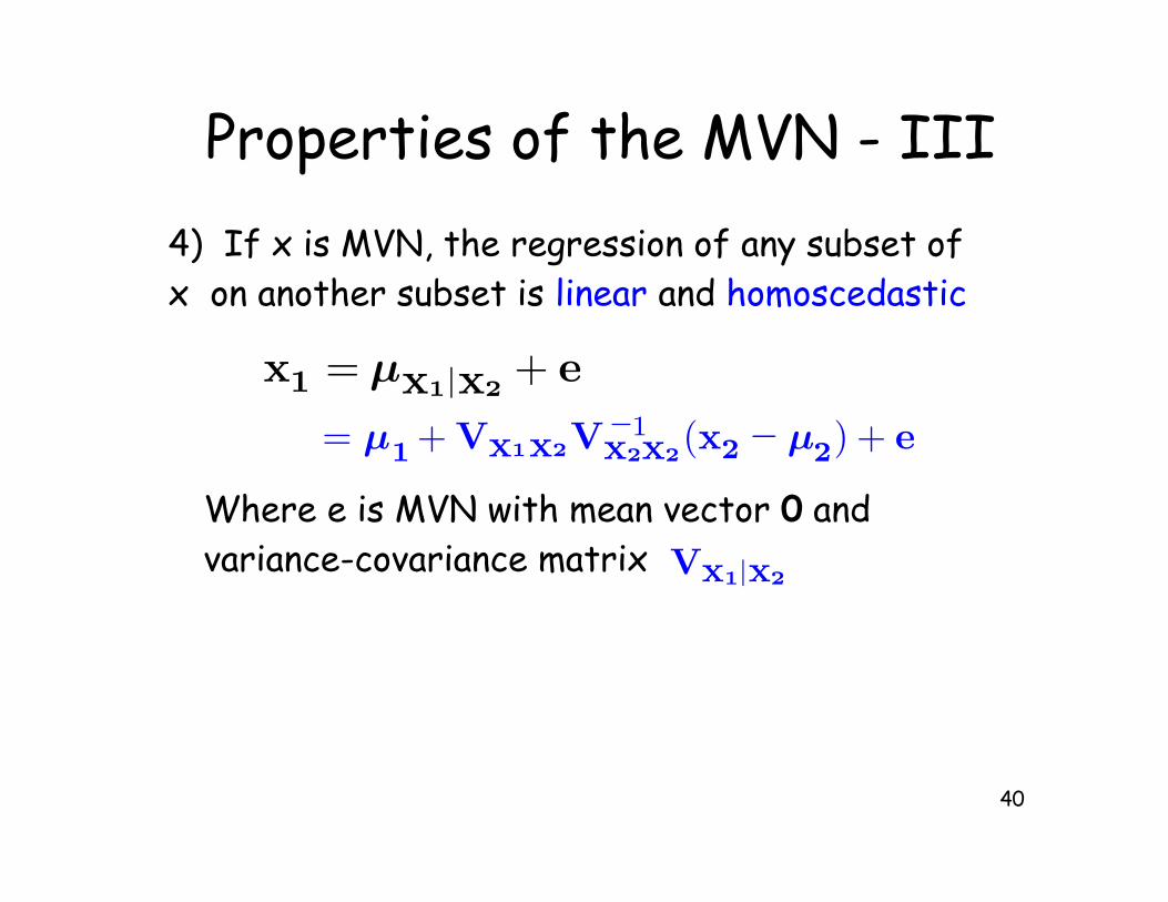
Properties of the MVN - III

4) If x is MVN, the regression of any subset of x on another subset is linear and homoscedastic

Where e is MVN with mean vector 0 andvariance-covariance matrix Vx1|x2

x1 = µx1 x2+ e|

= µ1 + Vx1x2V−1x2x2

(x2 − µ2) + e

41

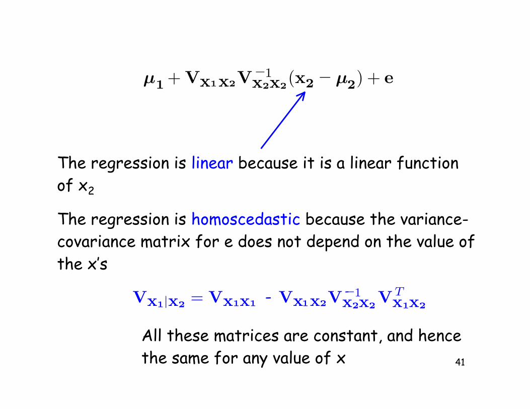
The regression is linear because it is a linear functionof x2

µ1 + Vx1x2V−1x2x2

(x2 − µ2) + e

The regression is homoscedastic because the variance-covariance matrix for e does not depend on the value of the x’s

--Vx1|x2= Vx1x1 Vx1x2V

−1x2x2

VTx1x2

All these matrices are constant, and hencethe same for any value of x

42

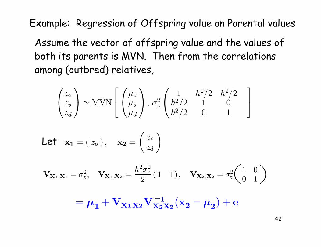
Example: Regression of Offspring value on Parental values

Assume the vector of offspring value and the values ofboth its parents is MVN. Then from the correlationsamong (outbred) relatives,

zo

zszd

∼MVN

µo

µs

µd

, σ2z

1 h2/2 h2/2

h2/2 1 0h2/2 0 1

Let x1 = ( zo ) , x2 =(

zs

zd

)

( )Vx1,x1 = σ2z, Vx1 ,x2 =

h2σ2z

2 ( 1 1 ) , Vx2,x2 = σ2z

1 00 1

= µ1 + Vx1x2V−1x2x2

(x2 − µ2) + e

43

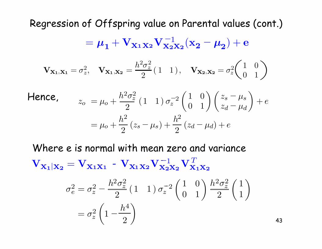
Regression of Offspring value on Parental values (cont.)

Hence,

Where e is normal with mean zero and variance

( ) ( )σ2

e = σ2z −

h2σ2z

2( 1 1 ) σ−2

z1 00 1

h2σ2z

211

= σ2z

(1− h4

2

)

-

zo = µo +h2σ2

z

2(1 1 ) σ−2

z

(1 00 1

)(zs − µs

zd− µd

)+ e

= µo +h2

2(zs−µs) +

h2

2(zd− µd) + e

= µ1 + Vx1x2V−1x2x2

(x2 − µ2) + e

( )Vx1,x1 = σ2z, Vx1 ,x2 = h2σ2

z

2( 1 1 ) , Vx2,x2 = σ2

z1 00 1

--Vx1|x2= Vx1x1 Vx1x2V

−1x2x2VT

x1x2

44

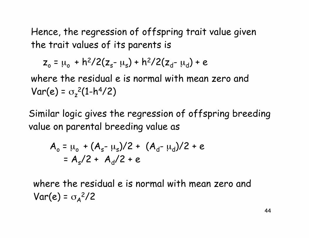
Hence, the regression of offspring trait value giventhe trait values of its parents is

zo = µo + h2/2(zs- µs) + h2/2(zd- µd) + e

where the residual e is normal with mean zero andVar(e) = &z

2(1-h4/2)

Similar logic gives the regression of offspring breedingvalue on parental breeding value as

Ao = µo + (As- µs)/2 + (Ad- µd)/2 + e = As/2 + Ad/2 + e

where the residual e is normal with mean zero andVar(e) = &A

2/2

45

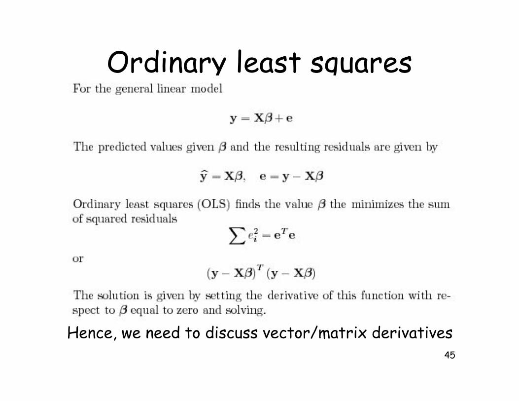
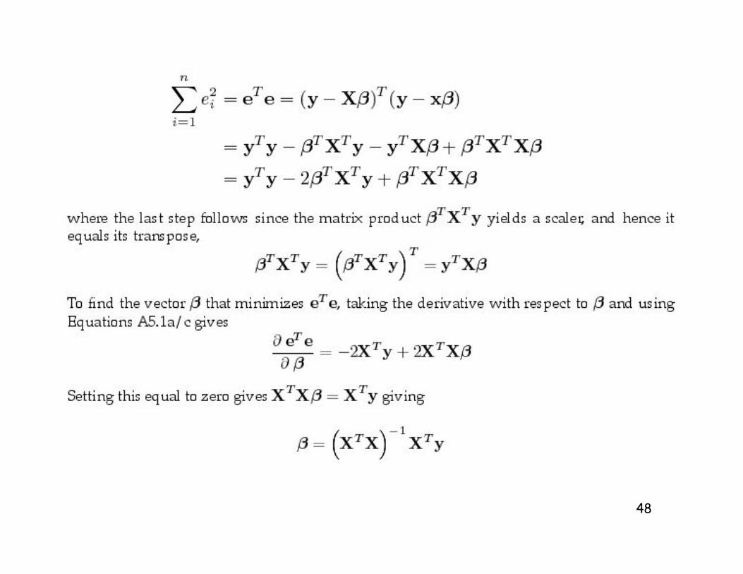
Ordinary least squares

Hence, we need to discuss vector/matrix derivatives

46

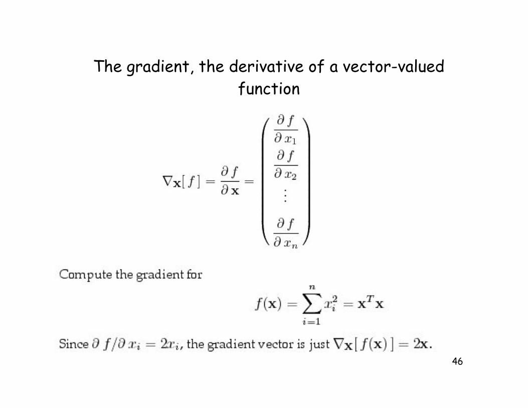
The gradient, the derivative of a vector-valuedfunction

47

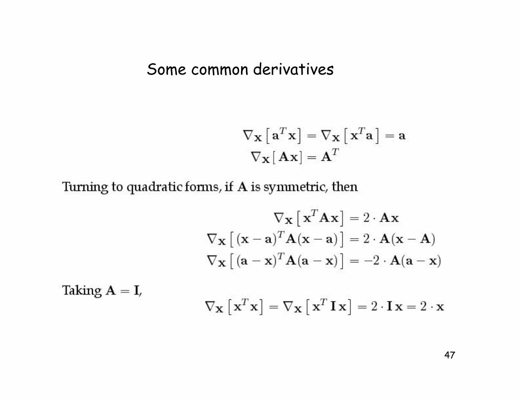
Some common derivatives

48

49

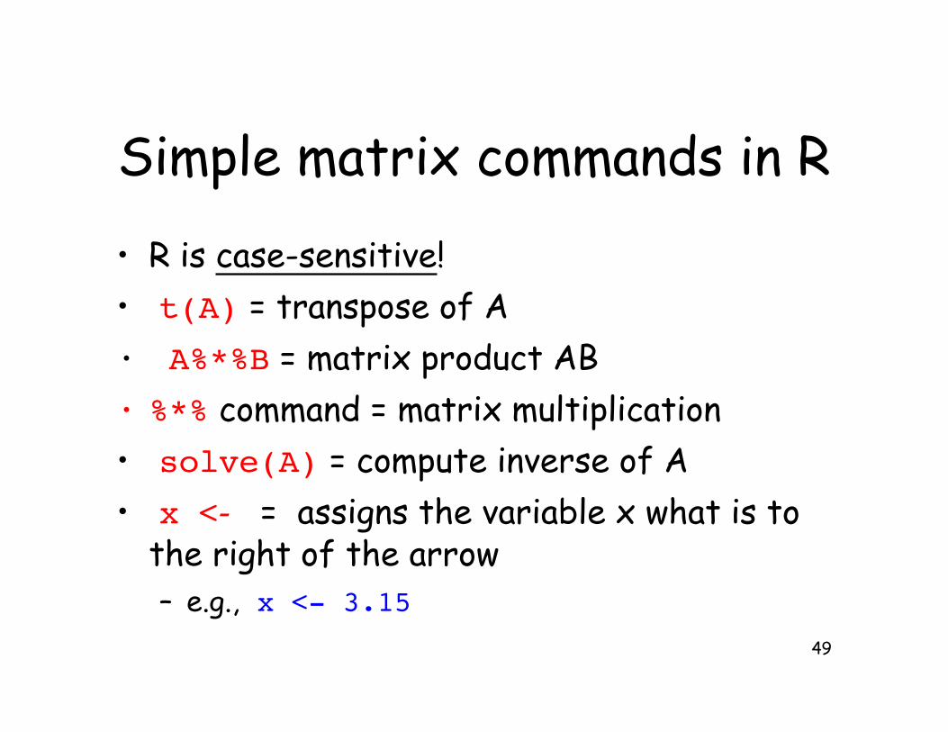
Simple matrix commands in R

• R is case-sensitive!

• t(A) = transpose of A

• A%*%B = matrix product AB

• %*% command = matrix multiplication

• solve(A) = compute inverse of A

• x <- = assigns the variable x what is tothe right of the arrow– e.g., x <- 3.15

50

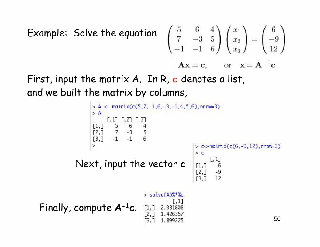
Example: Solve the equation

First, input the matrix A. In R, c denotes a list,and we built the matrix by columns,

Next, input the vector c

Finally, compute A-1c.

51

Example 2: Compute Var(y1), Var(y2), and Cov(y1,y2),where yi = ci

Tx.

c1TVc1

c2TVc2

c1TVc2

52

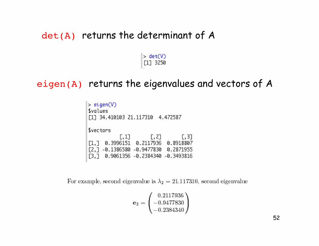
det(A) returns the determinant of A

eigen(A) returns the eigenvalues and vectors of A

53

Additional references

• Lynch & Walsh Chapter 8 (intro tomatrices)

• Matrix Calculations in R (to be emailed)

• Matrix Calculations in R (to be emailed)

• Online notes:

– Appendix 4 (Matrix geometry)

– Appendix 5 (Matrix derivatives)