Embed Size (px)
Citation preview

1
Lecture 20: Fitting geometric models

Announcements
• PS8 - PS10 will be a bit easier (and PS10 will be short) • Section this week: geometry tutorial • My office hours next Monday (11/16) are cancelled • Can chat in Friday OH instead, or by appointment
2

Today
• Finding correspondences • Fitting a homography • RANSAC
3
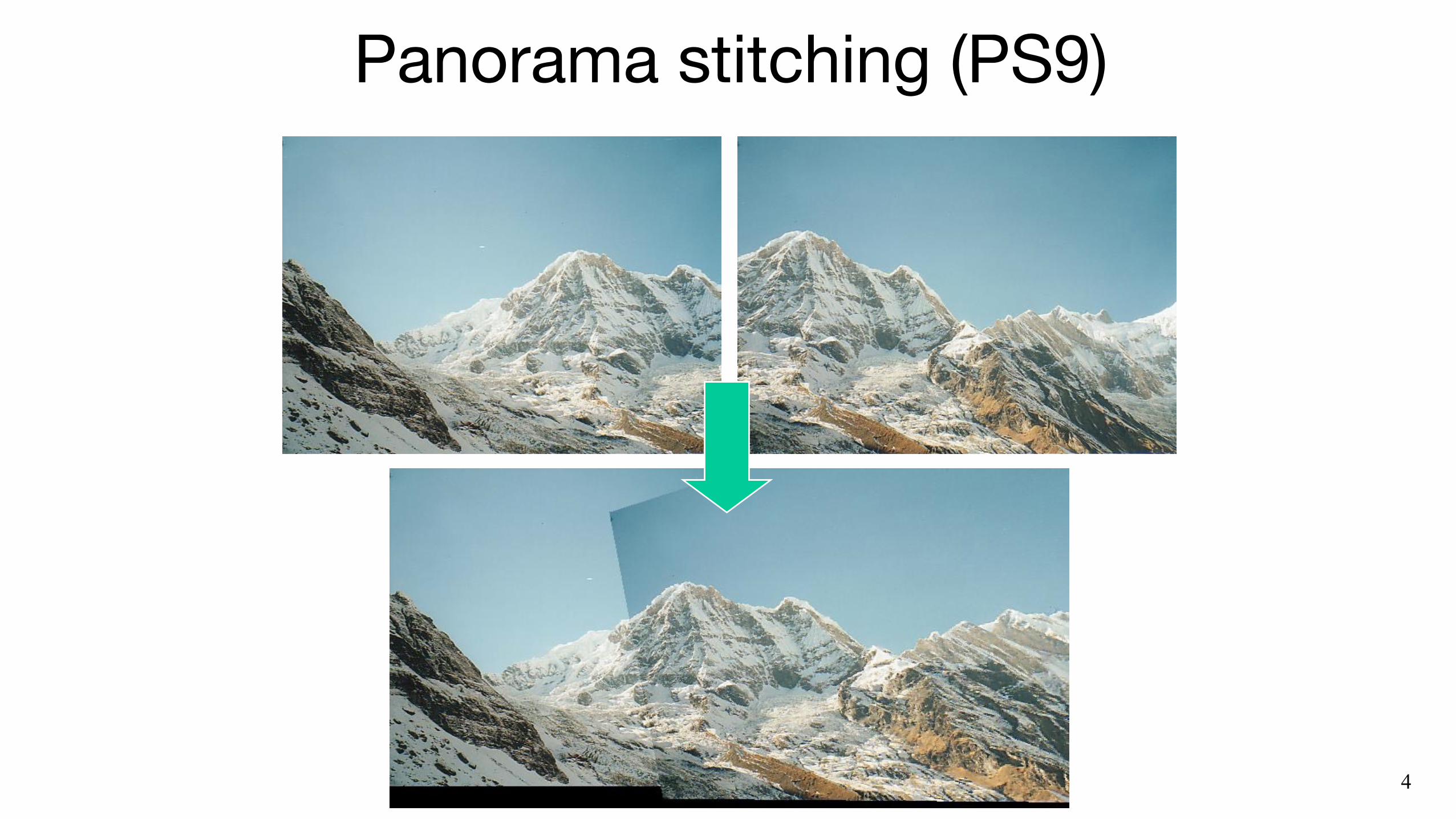
Panorama stitching (PS9)
4

Panorama stitching
5
Warp using homography

Panorama stitchingTo estimate the homography, we
need correspondences!
6
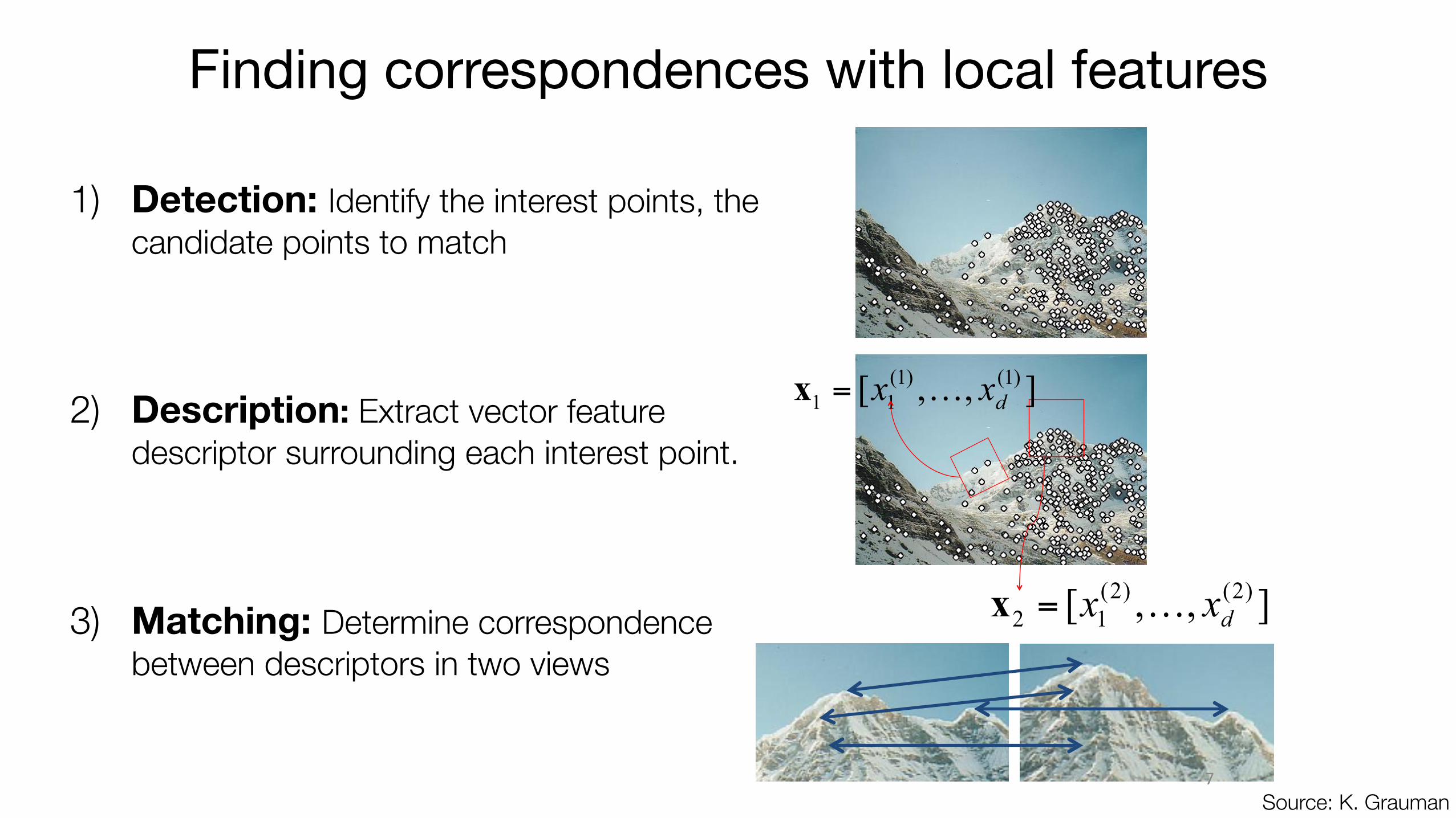
Finding correspondences with local features
1) Detection: Identify the interest points, the candidate points to match
2) Description: Extract vector feature descriptor surrounding each interest point.
3) Matching: Determine correspondence between descriptors in two views
],,[ )2()2(12 dxx …=x
Source: K. Grauman7
],,[ )1()1(11 dxx …=x

What are good regions to match?
“flat” region: no change in all directions
“edge”: no change along the edge direction
“corner”:significant change in all directions
• How does the window change when you shift it? • Shifting the window in any direction causes a big
change
Source: S. Seitz, D. Frolova, D. Simakov, N. Snavely8
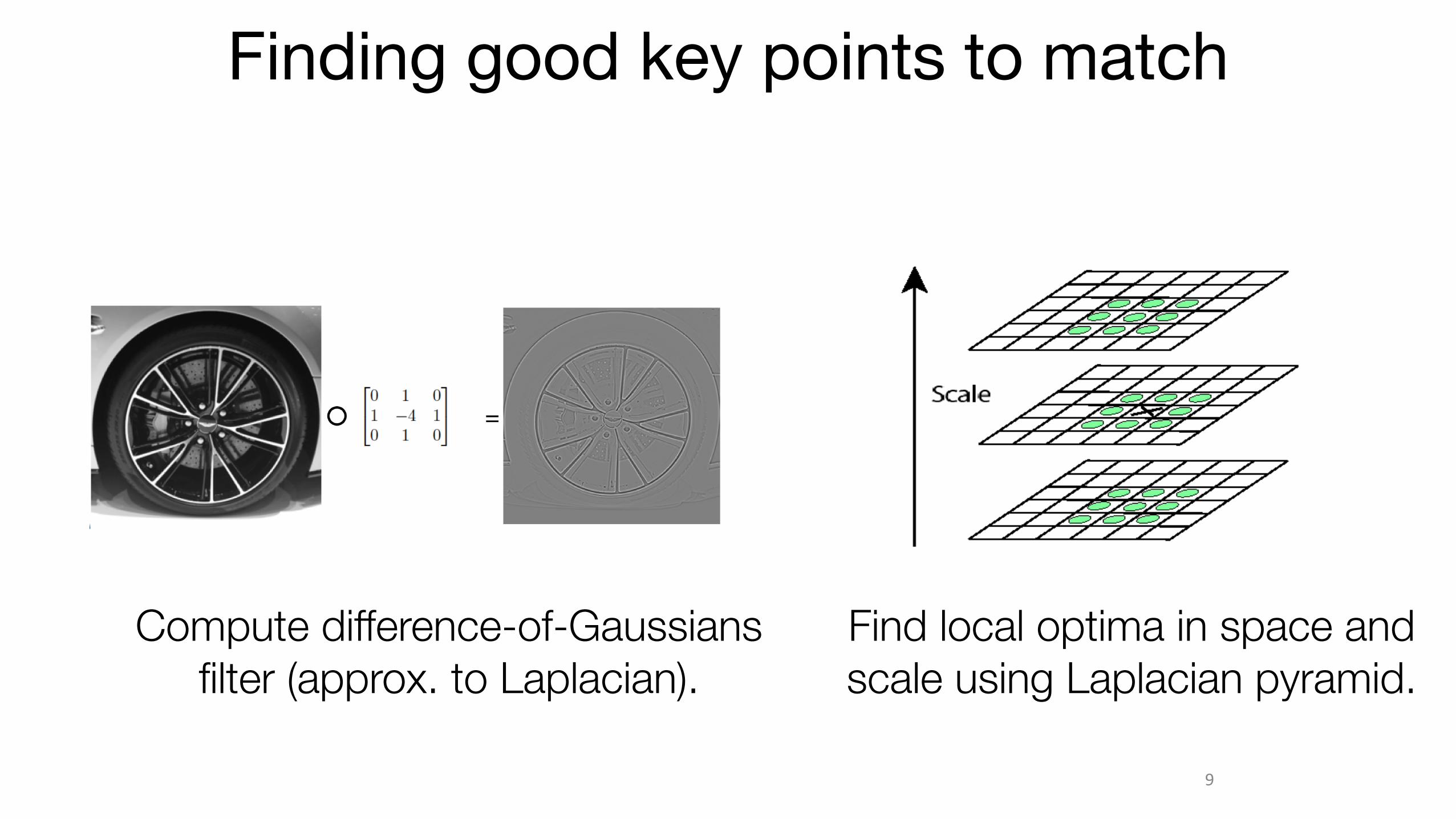
Finding good key points to match
Find local optima in space and scale using Laplacian pyramid.
Compute difference-of-Gaussians filter (approx. to Laplacian).
9
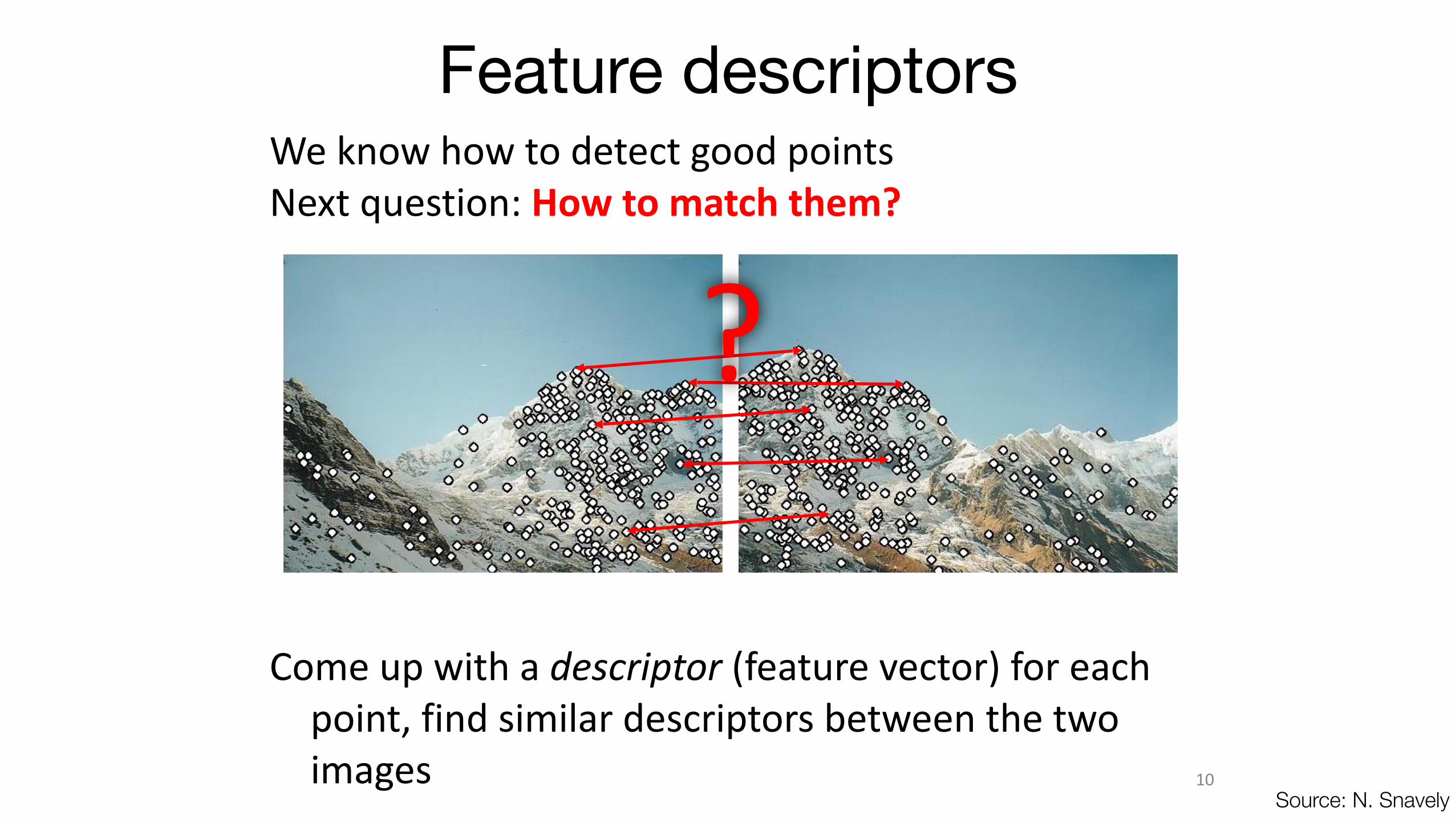
Feature descriptorsWe know how to detect good points Next question: How to match them?
Come up with a descriptor (feature vector) for each point, find similar descriptors between the two images
?
Source: N. Snavely10

CSE 576: Computer Vision
Take 40x40 window around feature • Find dominant orientation • Rotate to horizontal • Downsample to 8x8 • Intensity normalize the window by
subtracting the mean, dividing by the standard deviation in the window
Simple idea: normalized image patch
8 pixels40 pixels
Source: N. Snavely, M. Brown11
We want invariance to rotation, lighting, and tiny spatial shifts.
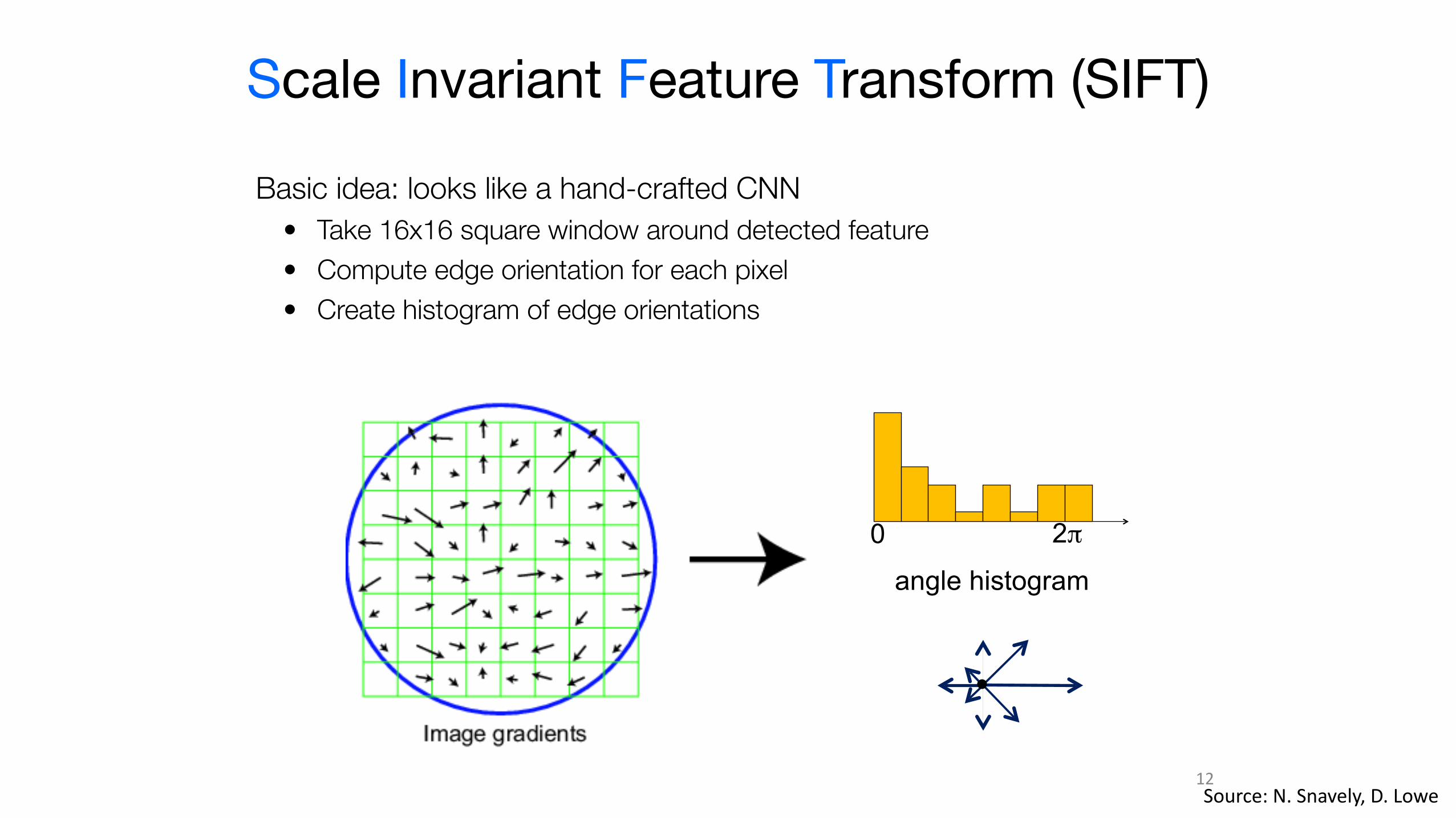
Basic idea: looks like a hand-crafted CNN • Take 16x16 square window around detected feature • Compute edge orientation for each pixel • Create histogram of edge orientations
Scale Invariant Feature Transform (SIFT)
Source: N. Snavely, D. Lowe
0 2π
angle histogram
12

Create the descriptor: • Rotation invariance: rotate by “dominant” orientation • Spatial invariance: spatial pool to 2x2 • Compute an orientation histogram for each cell • (4 x 4) cells x 8 orientations = 128 dimensional descriptor
Scale Invariant Feature Transform
Source: N. Snavely, D. Lowe13

SIFT invariances
Source: N. Snavely14

Today
• Finding correspondences • Computing local features • Matching
• Fitting a homography • RANSAC
15

How can we tell if two features match?
Source: N. Snavely16
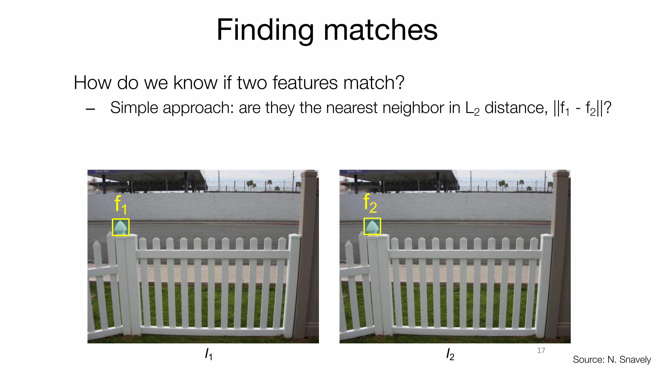
Finding matchesHow do we know if two features match?
– Simple approach: are they the nearest neighbor in L2 distance, ||f1 - f2||?
I1 I2
f1 f2
Source: N. Snavely17

Finding matchesHow do we know if two features match?
– Simple approach: are they the nearest neighbor in L2 distance, ||f1 - f2||? – Can give good scores to ambiguous (incorrect) matches
I1 I2
f1 f2
Source: N. Snavely18

f1 f2f2'
Finding matchesThrow away matches that fail tests:
• Ratio test: this by far the best match? • Ratio distance = ||f1 - f2 || / || f1 - f2’ || • f2 is best SSD match to f1 in I2 • f2’ is 2nd best SSD match to f1 in I2
• Forward-backward consistency: f1 should also be nearest neighbor of f2
I1 I2 Source: N. Snavely19

Feature matching example
51 feature matches after ratio test
Source: N. Snavely20

Feature matching example
58 feature matches after ratio test
Source: N. Snavely21

Today
• Finding correspondences • Computing local features • Matching
• Fitting a homography • RANSAC
22
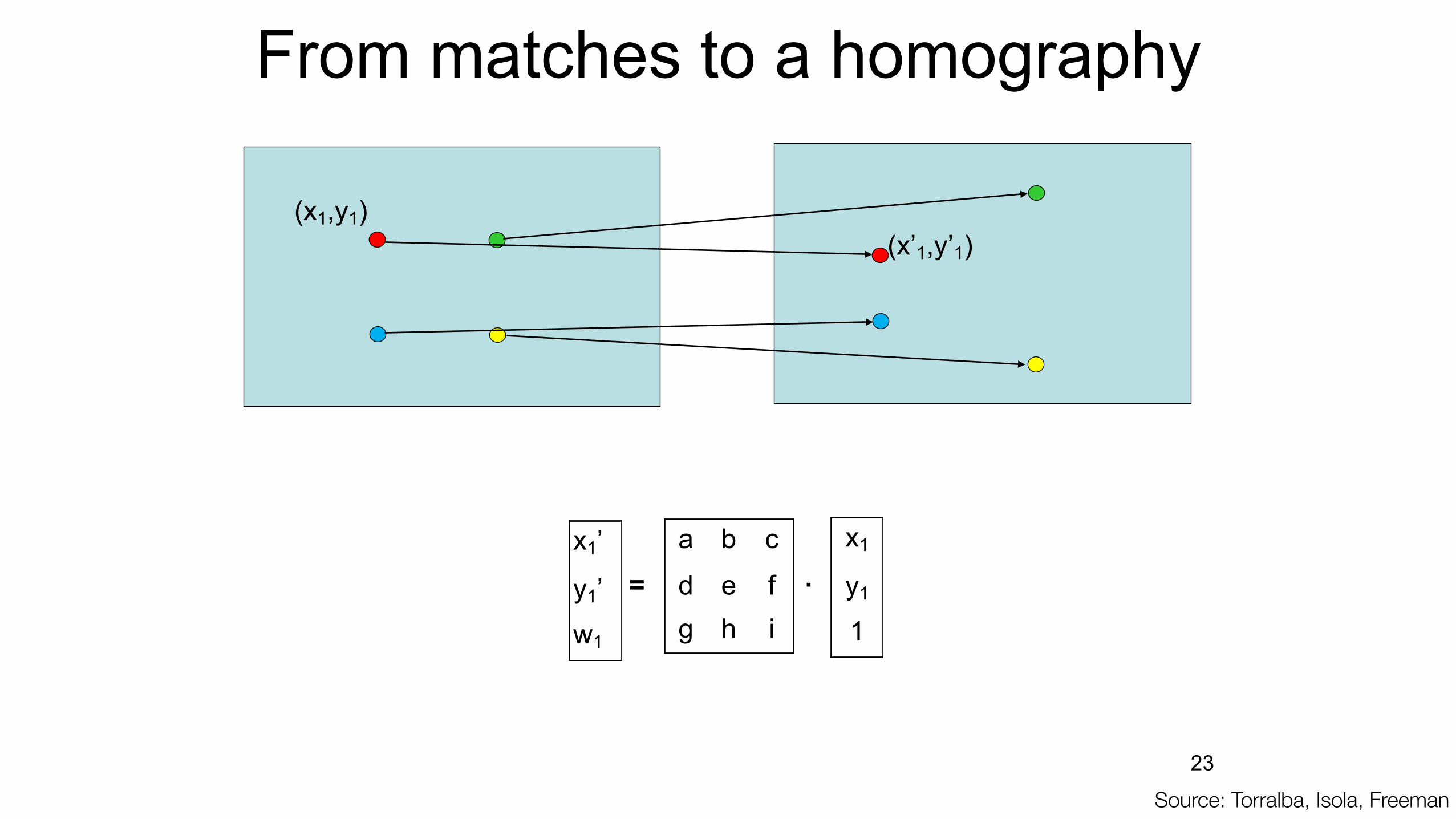
From matches to a homography
x1’
y1’w1
=
x1
y1
1
a b c
d e fg h i
.
(x1,y1)(x’1,y’1)
Source: Torralba, Isola, Freeman23

24
From matches to a homographyPoint in 1st image
J(H) =X
i
||fH(pi)� p0i||2
fH(pi) = Hpi/(HT
3 pi)
Matched point in 2nd
where applies homography (remember: homogenous coordinates)
minimize

25
x1’
y1’w1
=
x1
y1
1
a b c
d e fg h i
.
x1’=ax1 + by1+cgx1 + hy1+i
y1’=dx1 + ey1+fgx1 + hy1+i
gx1x’1 + hy1x’1+ix1’ = ax1 + by1+c
gx1y’1 + hy1y’1+ix1’ = dx1 + ey1+f
Going to heterogeneous coordinates:
Re-arranging the terms:
Option #1: Direct linear transform
Source: Torralba, Freeman, Isola

26
gx1x’1 + hy1x’1+ix1’ = ax1 + by1+c
gx1y’1 + hy1y’1+ix1’ = dx1 + ey1+f
Re-arranging the terms:gx1x’1 + hy1x’1+ix’1 - ax1 - by1- c = 0gx1y’1 + hy1y’1+iy’1 - dx1 - ey1- f = 0
-x1 -y1 -1 0 0 0 x1x’1 y1x’1 x’1 a b cd e fg h i
In matrix form. Can solve using Singular Value Decomposition (SVD).
0 0 0 -x1 -y1 -1 x1y’1 y1y’1 y’1
0 0=
Option #1: Direct linear transform
Fast to solve (but not using “right” loss function). Uses an algebraic trick.Often used in practice for initial solutions!
Source: Torralba, Freeman, Isola

21
0-1
x-2
Peaks
-3-3
-2y
-1
0
1
2
Option #2: Optimization
H
27
J(H)
J(H) =X
i
||fH(pi)� p0i||2
H11 H12
minimize

Optimization
28
J(H) =X
i
||fH(pi)� p0i||2minimize
• Can use gradient descent, just like when learning neural nets
• The problem is smaller scale than deep learning but has more local optima:
• Use 2nd derivatives to improve optimization
• Can use finite differences or autodiff
• Can use special-purpose nonlinear least squares methods.
• Exploits structure in the problem for a sum-of-squares loss.
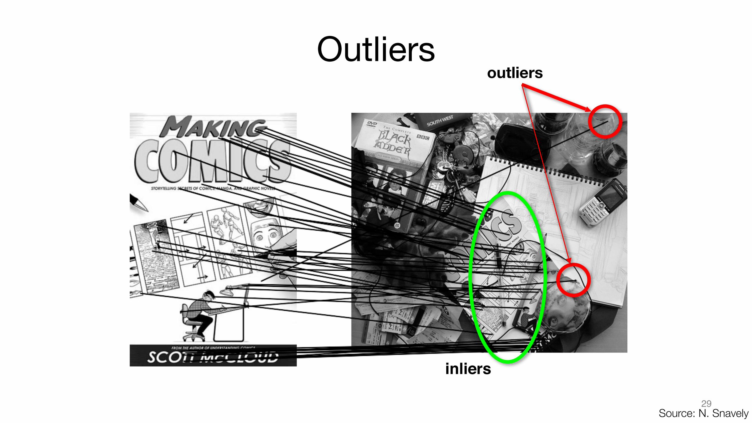
Outliersoutliers
inliers
29Source: N. Snavely

One idea: robust loss functions
30
minimize J(H) =N
∑i=1
2
∑j=1
ρ( fH(pi)j − p′�ij)
where is a robust loss.ρ(x)
Special case: is L2 loss (same as before)ρ(x) = x2

Robust loss functions
31ρ(x) = |x |L1 loss:
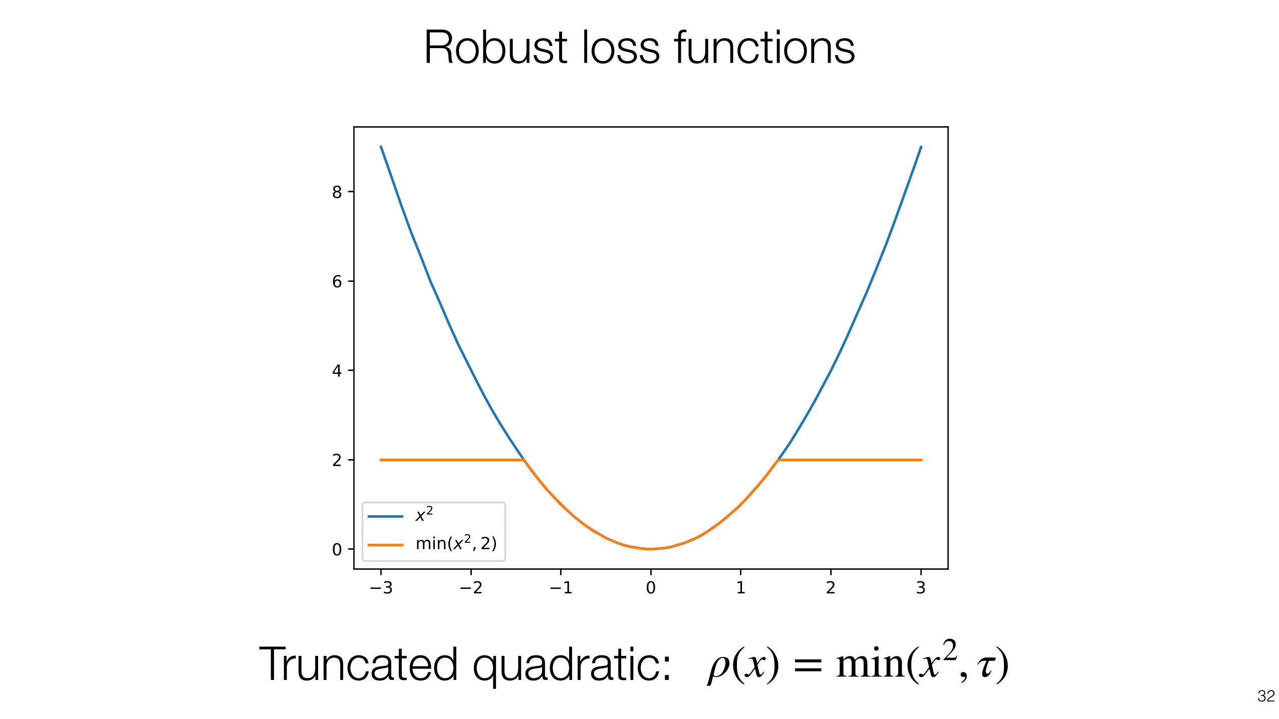
Robust loss functions
32ρ(x) = min(x2, τ)Truncated quadratic:

Robust loss functions
33
Huber loss:
ρ(x) =12 x2 if |x | ≤ τ,
τ( |x | − 12 τ), else

Robust loss functions
34Source: [Barron 2019, “A General and Adaptive Robust Loss Function”]
x

Handling outliers• Can be hard to fit robust loss
• Can be low, or get stuck in bad local minima • Let’s consider the problem of linear regression
Problem: Fit a line to these data points Least squares fit35
Source: N. Snavely
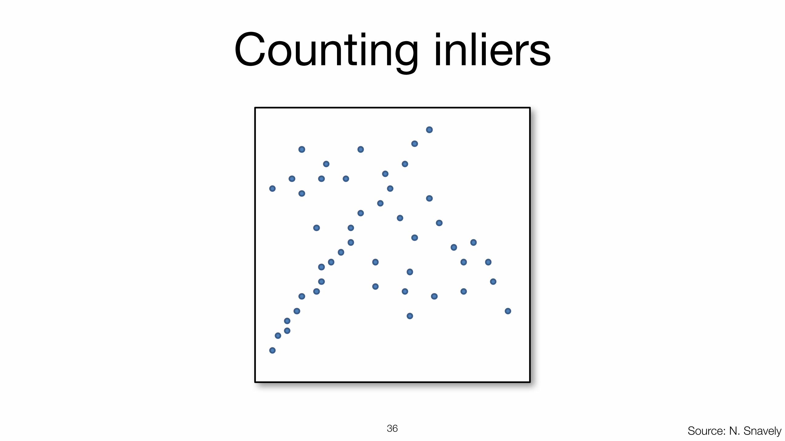
Counting inliers
36 Source: N. Snavely

Counting inliers
37
Inliers: 3Source: N. Snavely
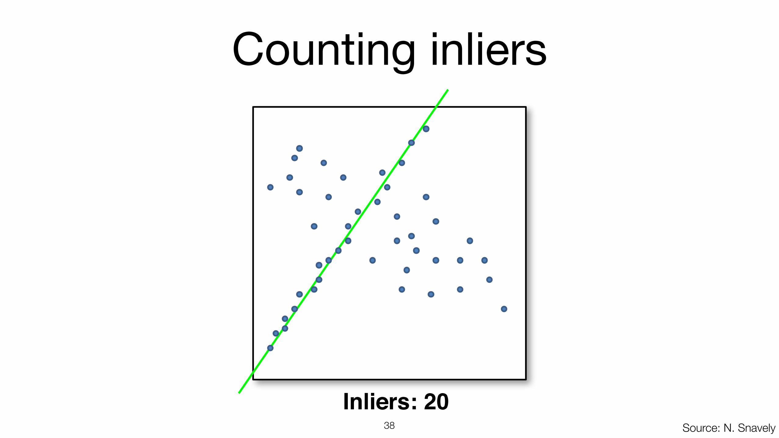
38
Inliers: 20Source: N. Snavely
Counting inliers

RANSAC
• Idea: – All the inliers will agree with each other on the
solution; the (hopefully small) number of outliers will (hopefully) disagree with each other • RANSAC only has guarantees if there are < 50% outliers
– “All good matches are alike; every bad match is bad in its own way.”
– Tolstoy via Alyosha Efros
Source: N. Snavely

RANSAC: random sample consensus
RANSAC loop (for N iterations): • Select four feature pairs (at random) • Compute homography H • Count inliers where ||pi’ - H pi|| < ε
Afterwards: • Choose H with largest set of inliers • Recompute H using only those inliers (often
using high-quality nonlinear least squares)40
Source: Torralba, Freeman, Isola

41
Simple example: fit a line
• Rather than homography H (8 numbers) fit y=ax+b (2 numbers a, b) to 2D pairs
Source: Torralba, Freeman, Isola

42
Simple example: fit a line
• Pick 2 points • Fit line • Count inliers
3 inlier
Source: Torralba, Freeman, Isola

43
Simple example: fit a line
• Pick 2 points • Fit line • Count inliers
4 inlier
Source: Torralba, Freeman, Isola

44
Simple example: fit a line
• Pick 2 points • Fit line • Count inliers
9 inlier
Source: Torralba, Freeman, Isola

45
Simple example: fit a line
• Pick 2 points • Fit line • Count inliers
8 inlier
Source: Torralba, Freeman, Isola

46
Simple example: fit a line
• Use biggest set of inliers • Do least-square fit
Source: Torralba, Freeman, Isola

Example: fitting a translation
Source: N. Snavely

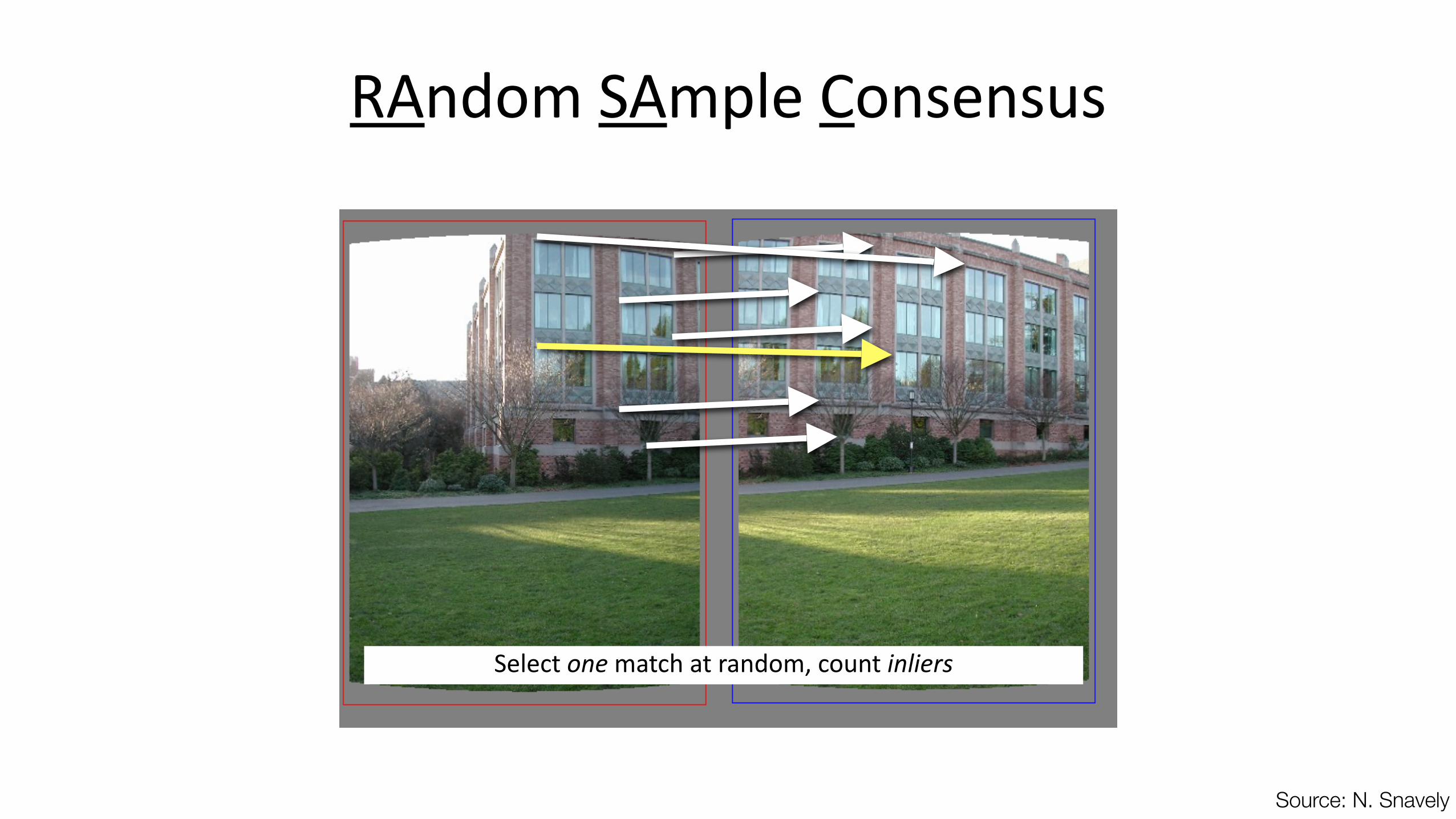
RAndom SAmple Consensus
Select one match at random, count inliers
Source: N. Snavely
RAndom SAmple Consensus
Select one match at random, count inliers
Source: N. Snavely

RAndom SAmple Consensus
Select one match at random, count inliers
Source: N. Snavely

RAndom SAmple Consensus
Select another match at random, count inliers
Source: N. Snavely

RAndom SAmple Consensus
Select another match at random, count inliers
Source: N. Snavely

RAndom SAmple Consensus
Choose the translation with the highest number of inliers
Source: N. Snavely
Then compute average translation, using only inliers

Warping with a homography (PS9)1. Compute features using SIFT
2. Match features
3. Compute homography using RANSAC
54Source: N. Snavely

Next class: more 3D