1

Data Compression Audio compression

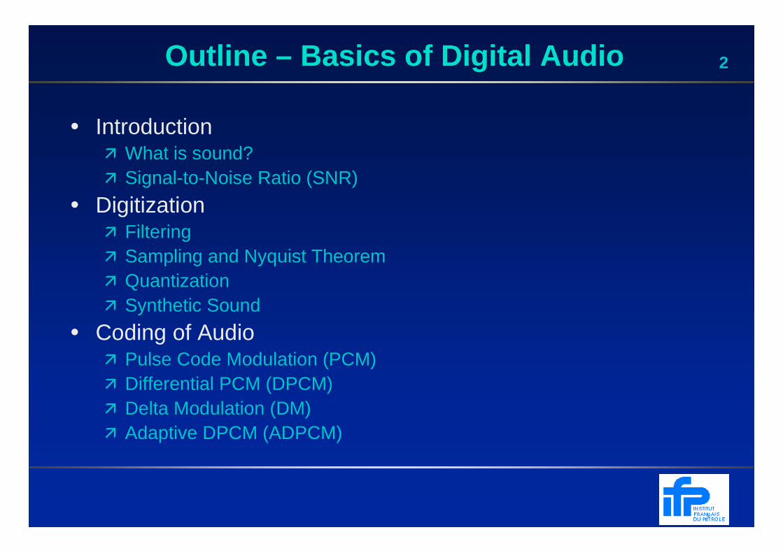
2Outline – Basics of Digital Audio

• Introduction� What is sound? � Signal-to-Noise Ratio (SNR)

• Digitization� Filtering� Sampling and Nyquist Theorem� Quantization� Synthetic Sound

• Coding of Audio� Pulse Code Modulation (PCM)� Differential PCM (DPCM)� Delta Modulation (DM)� Adaptive DPCM (ADPCM)

3What is sound?

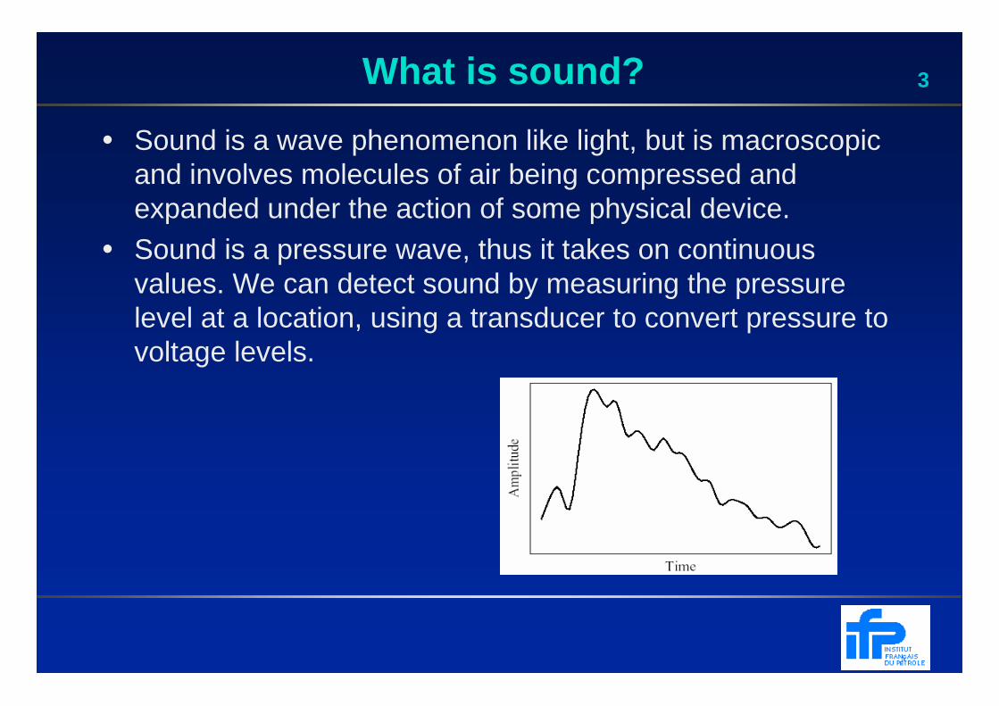
• Sound is a wave phenomenon like light, but is macroscopic and involves molecules of air being compressed and expanded under the action of some physical device.

• Sound is a pressure wave, thus it takes on continuous values. We can detect sound by measuring the pressure level at a location, using a transducer to convert pressure to voltage levels.

4Signal to Noise Ratio (SNR)

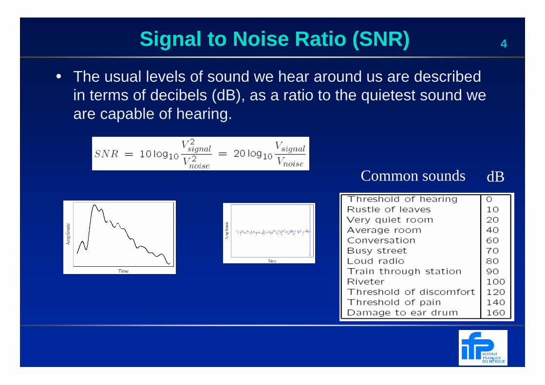
• The usual levels of sound we hear around us are described in terms of decibels (dB), as a ratio to the quietest sound we are capable of hearing.

dBCommon sounds

Vsignal Vnoise

5Digitization

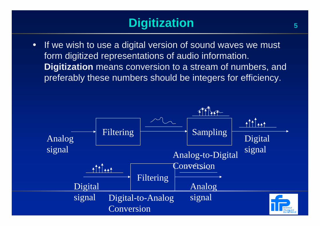
• If we wish to use a digital version of sound waves we must form digitized representations of audio information.Digitization means conversion to a stream of numbers, and preferably these numbers should be integers for efficiency.

Filtering Sampling

Filtering

Analog-to-Digital Conversion

Digital-to-Analog Conversion

Digital signal

Analog signal

Digital signal

Analog signal

6Filtering

• Prior to sampling and Analog-to-Digital conversion, the audio signal is also usually filtered to remove unwanted frequencies. The frequencies kept depend on the application:� For speech, typically from 50Hz to 10kHz is retained, and other frequencies

are blocked by the use of a band-pass filter that screens out lower and higher frequencies.

� An audio music signal will typically contain from about 20Hz up to 20kHz.

• At the Digital-to-Analog converter end, high frequencies may reappear in the output because of sampling and then quantization, smooth input signal is replaced by a series of step functions containing all possible frequencies.� So at the decoder side, a lowpass filter is used after the DA circuit.

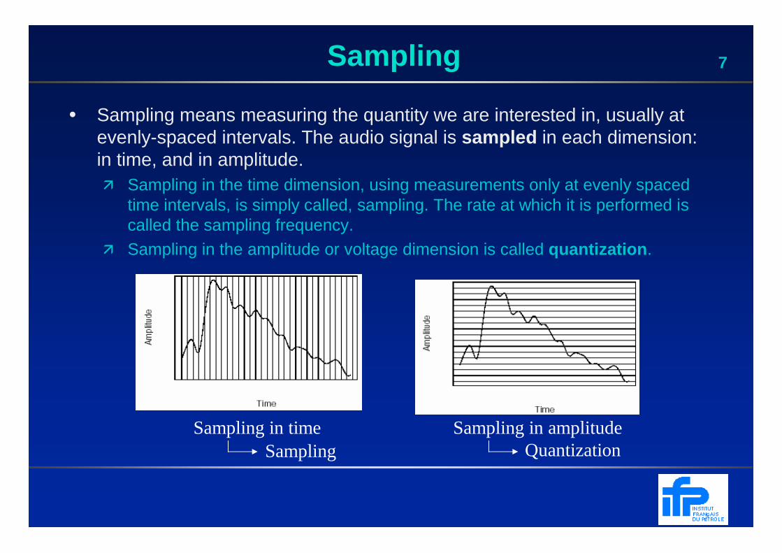
7Sampling

• Sampling means measuring the quantity we are interested in, usually at evenly-spaced intervals. The audio signal is sampled in each dimension: in time, and in amplitude. � Sampling in the time dimension, using measurements only at evenly spaced

time intervals, is simply called, sampling. The rate at which it is performed is called the sampling frequency.

� Sampling in the amplitude or voltage dimension is called quantization .

Sampling in time Sampling in amplitudeSampling Quantization

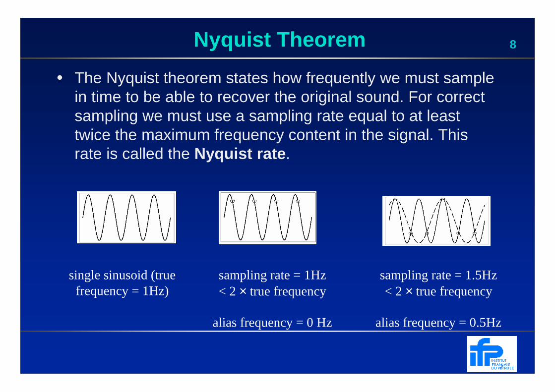
8Nyquist Theorem

• The Nyquist theorem states how frequently we must sample in time to be able to recover the original sound. For correct sampling we must use a sampling rate equal to at least twice the maximum frequency content in the signal. This rate is called the Nyquist rate .

single sinusoid (true frequency = 1Hz)

sampling rate = 1Hz < 2 × true frequency

alias frequency = 0 Hz

sampling rate = 1.5Hz < 2 × true frequency

alias frequency = 0.5Hz

9Nyquist Theorem (2)

• Nyquist frequency = half of the Nyquist rate.• Since it would be impossible to recover frequencies higher

than Nyquist frequency in any event, most systems have an antialiasing filter that restricts the frequency content in the input to the sampler to a range at or below Nyquistfrequency.

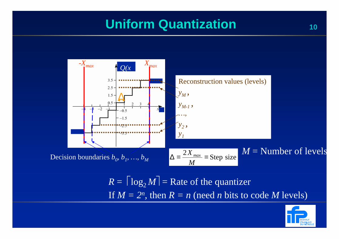
10Uniform Quantization

Q(x)

Xmax-Xmax

Decision boundariesb0, b1, …, bM

Reconstruction values (levels)

yM , yM-1 , …,

y2 , y1

∆

M = Number of levels

R= log2 M = Rate of the quantizerIf M = 2n, then R = n (need n bits to code M levels)

size Step 2 ==∆

M

X max

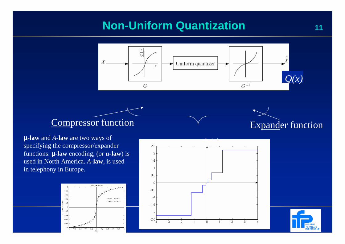
11Non-Uniform Quantization

Compressor function Expander function

Q(x)

x

Q(x)

µµµµ-law and A-law are two ways of specifying the compressor/expander functions. µµµµ-law encoding, (or u-law) is used in North America. A-law, is used in telephony in Europe.

12Data Rate Comparison

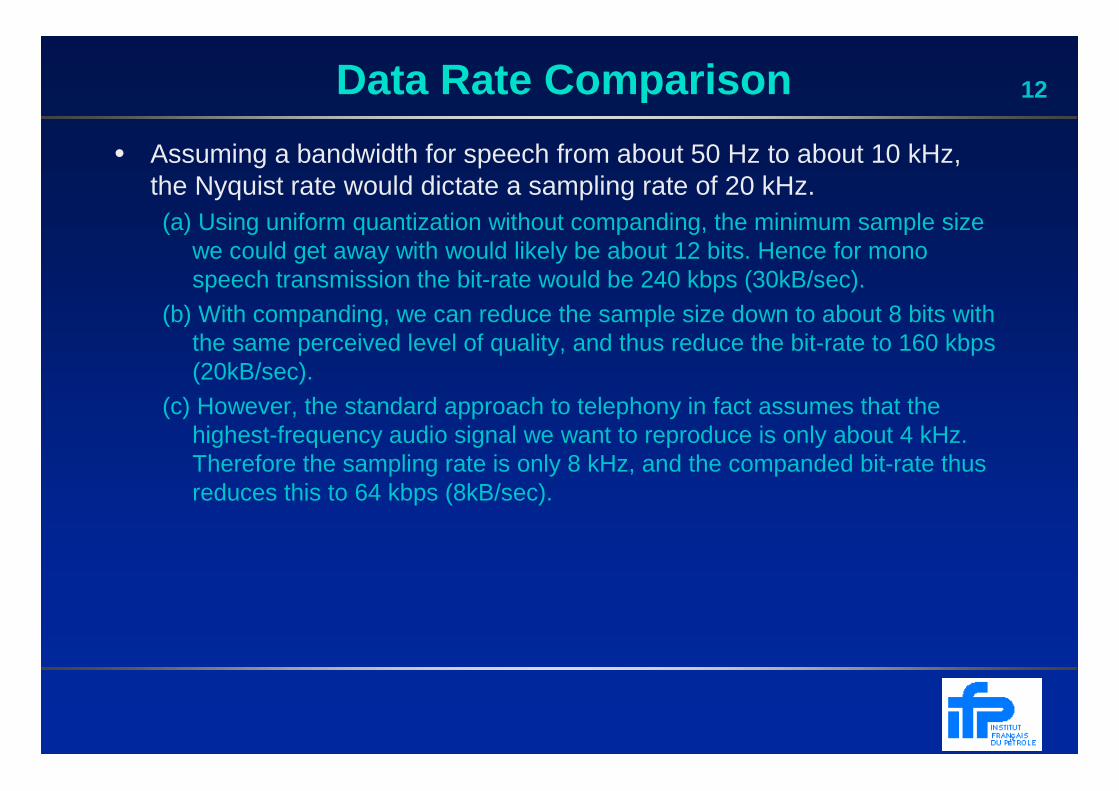
• Assuming a bandwidth for speech from about 50 Hz to about 10 kHz, the Nyquist rate would dictate a sampling rate of 20 kHz.(a) Using uniform quantization without companding, the minimum sample size

we could get away with would likely be about 12 bits. Hence for mono speech transmission the bit-rate would be 240 kbps (30kB/sec).

(b) With companding, we can reduce the sample size down to about 8 bits with the same perceived level of quality, and thus reduce the bit-rate to 160 kbps (20kB/sec).

(c) However, the standard approach to telephony in fact assumes that the highest-frequency audio signal we want to reproduce is only about 4 kHz.Therefore the sampling rate is only 8 kHz, and the companded bit-rate thus reduces this to 64 kbps (8kB/sec).

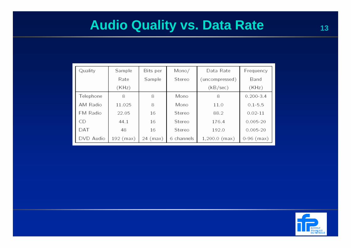
13Audio Quality vs. Data Rate

14Synthetic Sound

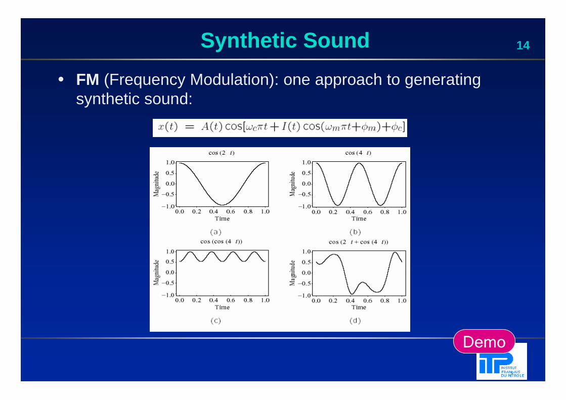
• FM (Frequency Modulation): one approach to generating synthetic sound:

Demo

15Synthetic Sound (2)

• Wave Table synthesis : A more accurate way of generating sounds from digital signals. Also known, simply, as sampling . In this technique, the actual digital samples of sounds from real instruments are stored. Since wave tables are stored in memory on the sound card, they can be manipulated by software so that sounds can be combined, edited, and enhanced.

16Coding of Audio

• Coding of Audio: Quantization and transformation of data are collectively known as coding of the data.

• In general, producing quantized sampled output for audio is called PCM (Pulse Code Modulation). The differences version is called DPCM (and a crude but efficient variant is called DM). The adaptive version is called ADPCM.

17Encoding/Decoding Scheme

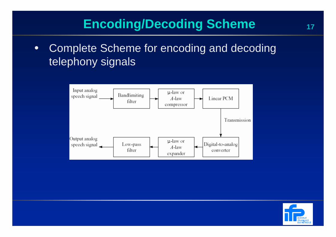
• Complete Scheme for encoding and decoding telephony signals

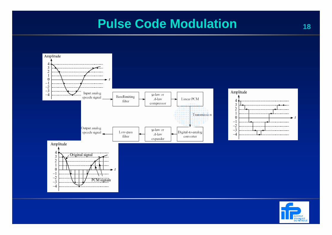
18Pulse Code Modulation

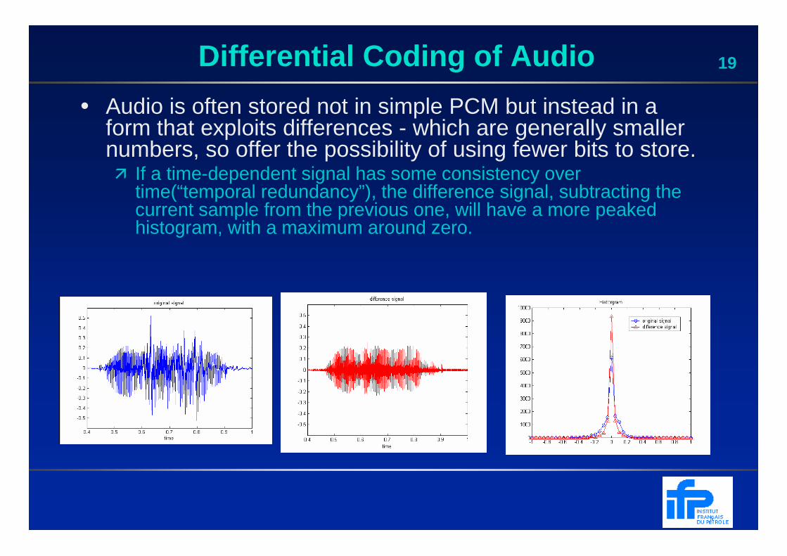
19Differential Coding of Audio

• Audio is often stored not in simple PCM but instead in a form that exploits differences - which are generally smaller numbers, so offer the possibility of using fewer bits to store.� If a time-dependent signal has some consistency over

time(“temporal redundancy”), the difference signal, subtracting the current sample from the previous one, will have a more peaked histogram, with a maximum around zero.

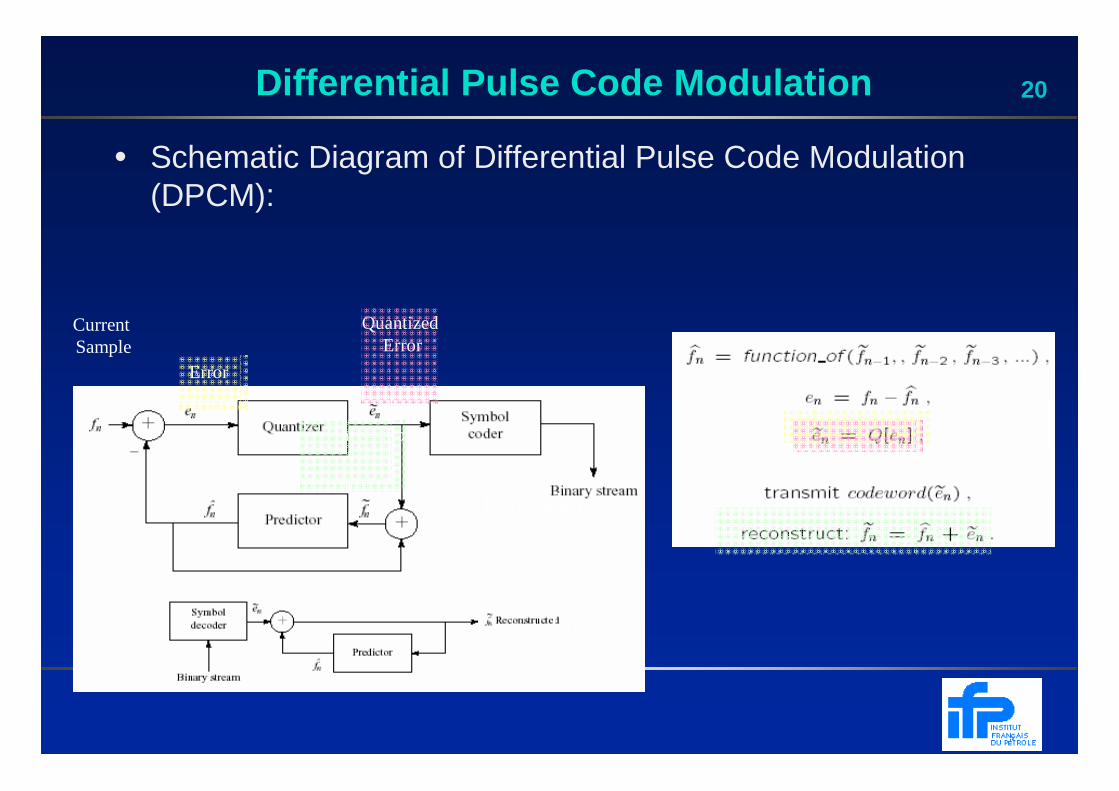
20Differential Pulse Code Modulation

• Schematic Diagram of Differential Pulse Code Modulation (DPCM):

Encoder

Decoder

Current Sample

Error

Quantized Error

Reconstruction

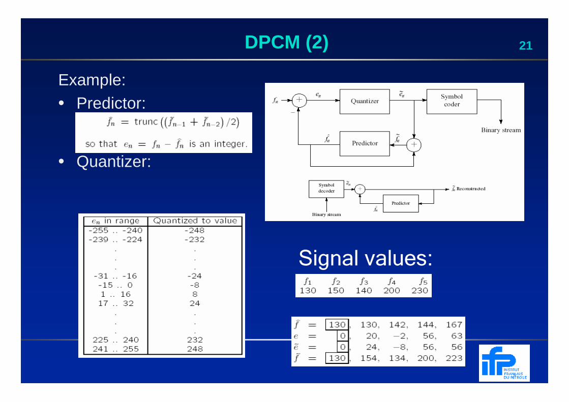
21DPCM (2)

Example:• Predictor:

• Quantizer:

Signal values:

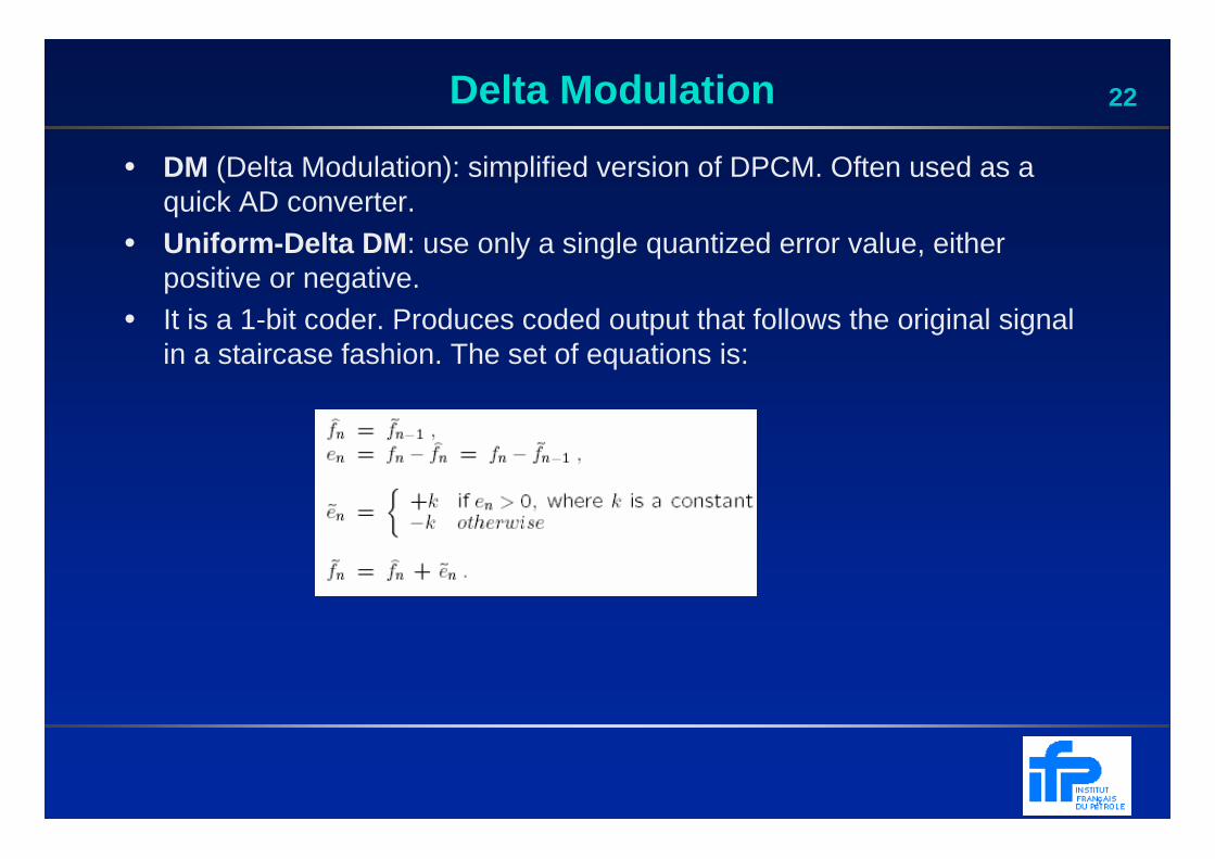
22Delta Modulation

• DM (Delta Modulation): simplified version of DPCM. Often used as a quick AD converter.

• Uniform -Delta DM : use only a single quantized error value, either positive or negative.

• It is a 1-bit coder. Produces coded output that follows the original signal in a staircase fashion. The set of equations is:

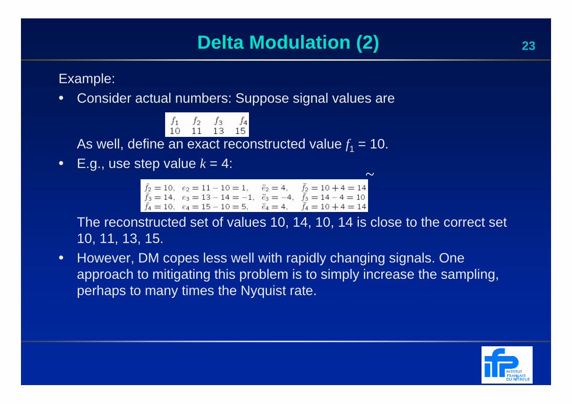
23Delta Modulation (2)

Example:• Consider actual numbers: Suppose signal values are

As well, define an exact reconstructed value f1 = 10.• E.g., use step value k = 4:

The reconstructed set of values 10, 14, 10, 14 is close to the correct set 10, 11, 13, 15.

• However, DM copes less well with rapidly changing signals. One approach to mitigating this problem is to simply increase the sampling, perhaps to many times the Nyquist rate.

~

24Adaptive DPCM (ADPCM)

• ADPCM (Adaptive DPCM) takes the idea of adapting the coder to suit the input much farther. The two pieces that make up a DPCM coder: the quantizer and the predictor.

� In Adaptive DM, adapt the quantizer step size to suit the input. In DPCM, we can change the step size as well as decision boundaries, using a non-uniform quantizer.

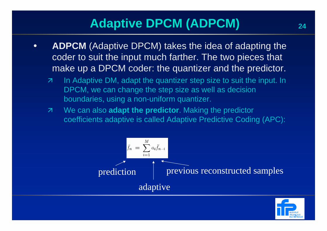
� We can also adapt the predictor . Making the predictor coefficients adaptive is called Adaptive Predictive Coding (APC):

prediction

adaptive

previous reconstructed samples

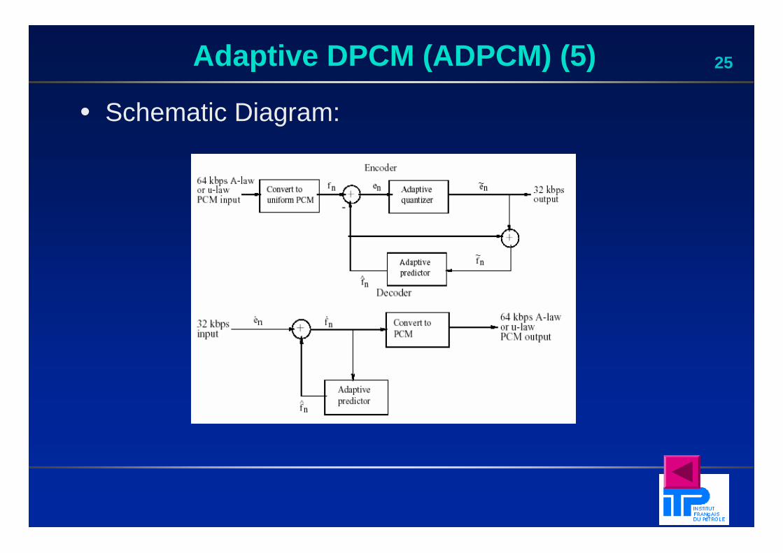
25Adaptive DPCM (ADPCM) (5)

• Schematic Diagram:

26Outline – Audio Compression

• Vocoder� Channel Vocoder� Formant Vocoder� Linear Predictive Coder (LPC)� Code Excited Linear Prediction (CELP)

• Psychoacoustics� Equal-Loudness Relations � Frequency Masking� Temporal Masking

• MPEG Audio� MPEG-1� Brief introduction of MPEG-2, MPEG-4 and MPEG-7

27Vocoders

• Vocoders - voice coders, which cannot be usefully applied when other analog signals, such as modem signals, are in use.� concerned with modeling speech so that the salient

features are captured in as few bits as possible.� use either a model of the speech waveform in time (LPC

(Linear Predictive Coding) vocoding), or break down the signal into frequency components and model these (channel vocoders and formant vocoders).

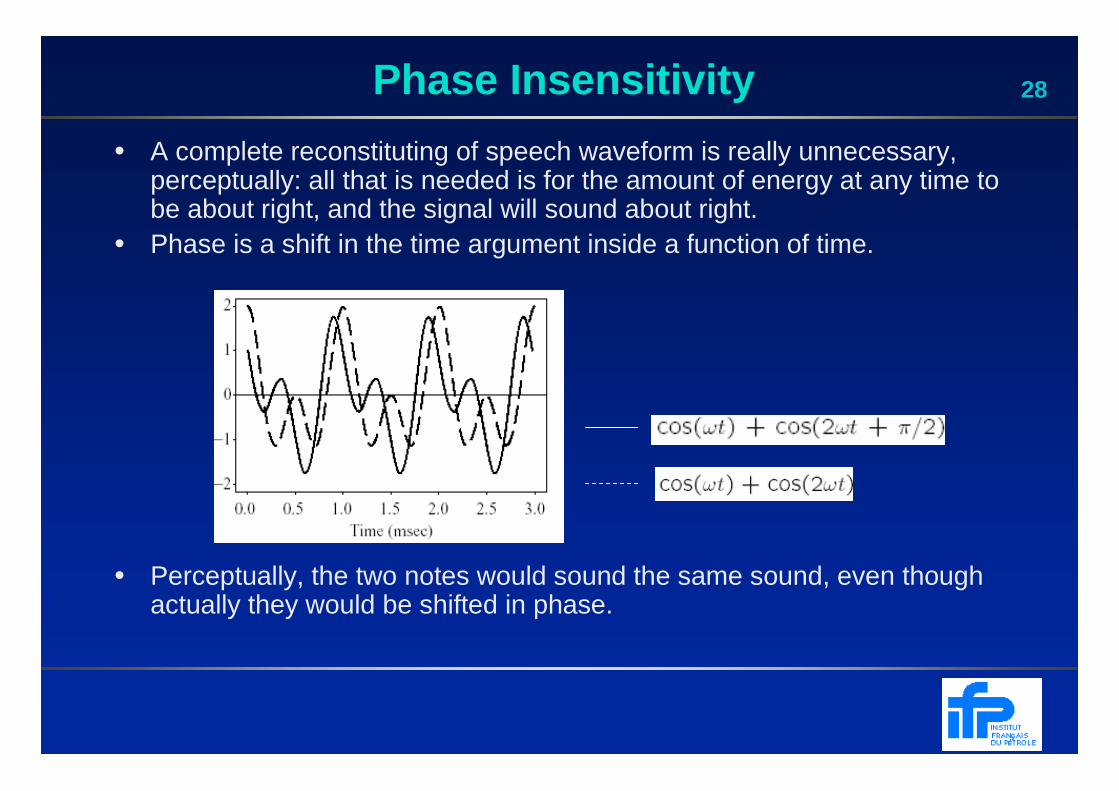
28Phase Insensitivity

• A complete reconstituting of speech waveform is really unnecessary, perceptually: all that is needed is for the amount of energy at any time to be about right, and the signal will sound about right.

• Phase is a shift in the time argument inside a function of time.

• Perceptually, the two notes would sound the same sound, even though actually they would be shifted in phase.

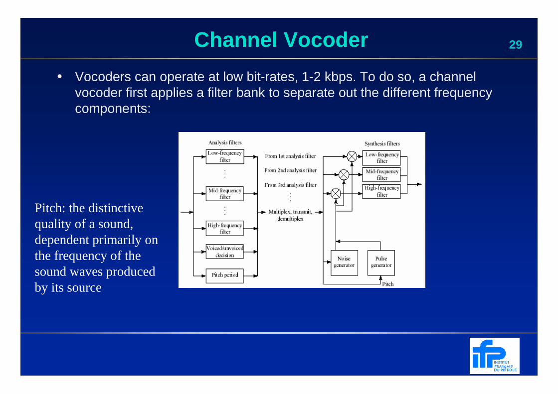
29Channel Vocoder

• Vocoders can operate at low bit-rates, 1-2 kbps. To do so, a channel vocoder first applies a filter bank to separate out the different frequency components:

Pitch: the distinctive quality of a sound, dependent primarily on the frequency of the sound waves produced by its source

30Linear Predictive Coding (LPC)

• LPC vocoders extract salient features of speech directly from the waveform, rather than transforming the signal to the frequency domain

• LPC Features:� uses a time-varying model of vocal tract sound generated from a

given excitation � transmits only a set of parameters modeling the shape and excitation

of the vocal tract, not actual signals or differences

→ small bit-rate

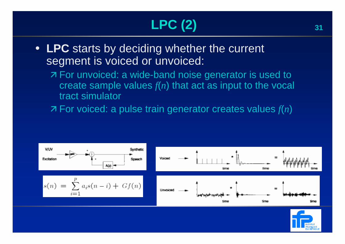
31LPC (2)

• LPC starts by deciding whether the current segment is voiced or unvoiced:� For unvoiced: a wide-band noise generator is used to

create sample values f(n) that act as input to the vocal tract simulator

� For voiced: a pulse train generator creates values f(n)

32Code Excited Linear Prediction (CELP)

• CELP is a more complex family of coders that attempts to mitigate the lack of quality of the simple LPC model

• CELP uses a more complex description of the excitation:� An entire set (a codebook) of excitation vectors is matched to the

actual speech, and the index of the best match is sent to the receiver� The complexity increases the bit-rate to 4,800-9,600 bps� The resulting speech is perceived as being more similar and

continuous� Quality achieved this way is sufficient for audio conferencing

33CELP (2)

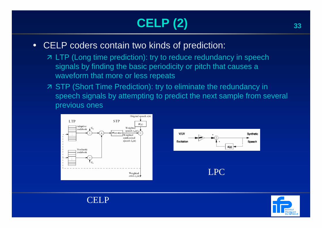
• CELP coders contain two kinds of prediction:� LTP (Long time prediction): try to reduce redundancy in speech

signals by finding the basic periodicity or pitch that causes a waveform that more or less repeats

� STP (Short Time Prediction): try to eliminate the redundancy in speech signals by attempting to predict the next sample from several previous ones

CELP

LPC

34Psychoacoustics

• Equal-Loudness Relations� Fletcher-Munson Curves� Threshold of Hearing

• Frequency Masking� Frequency Masking Curves� Critical Bands� Bark Unit

• Temporal Masking

35Equal-Loudness Relations

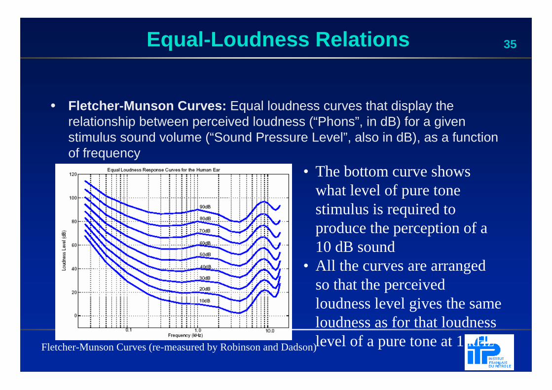
• Fletcher-Munson Curves: Equal loudness curves that display the relationship between perceived loudness (“Phons”, in dB) for a given stimulus sound volume (“Sound Pressure Level”, also in dB), as a function of frequency

Fletcher-Munson Curves (re-measured by Robinson and Dadson)

• The bottom curve shows what level of pure tone stimulus is required to produce the perception of a 10 dB sound

• All the curves are arranged so that the perceived loudness level gives the same loudness as for that loudness level of a pure tone at 1 kHz

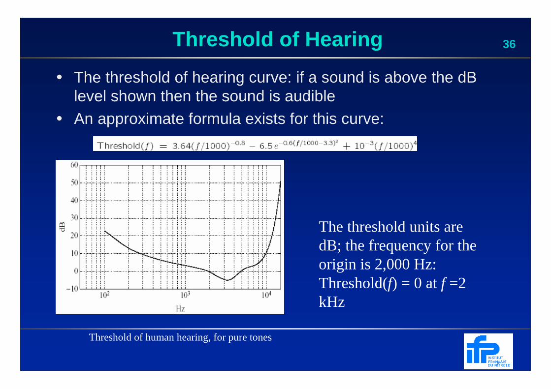
36Threshold of Hearing

Threshold of human hearing, for pure tones

The threshold units are dB; the frequency for the origin is 2,000 Hz: Threshold(f) = 0 at f =2 kHz

• The threshold of hearing curve: if a sound is above the dB level shown then the sound is audible

• An approximate formula exists for this curve:

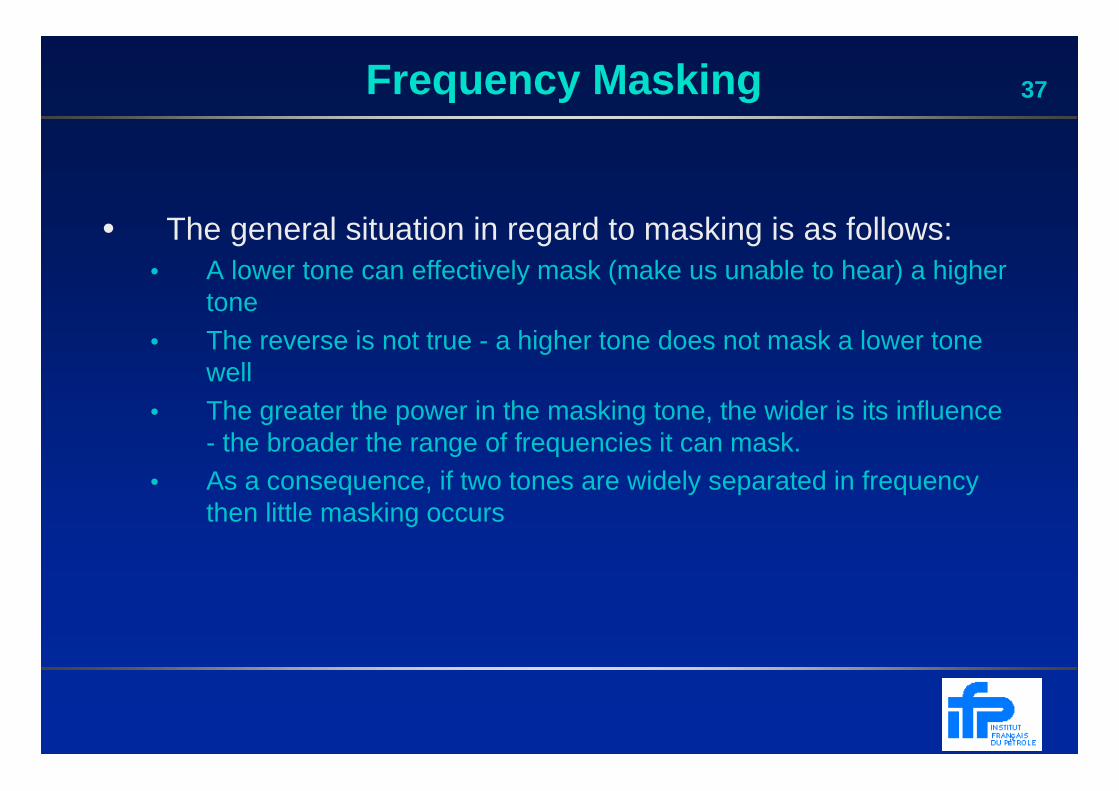
37Frequency Masking

• The general situation in regard to masking is as follows:• A lower tone can effectively mask (make us unable to hear) a higher

tone• The reverse is not true - a higher tone does not mask a lower tone

well• The greater the power in the masking tone, the wider is its influence

- the broader the range of frequencies it can mask.• As a consequence, if two tones are widely separated in frequency

then little masking occurs

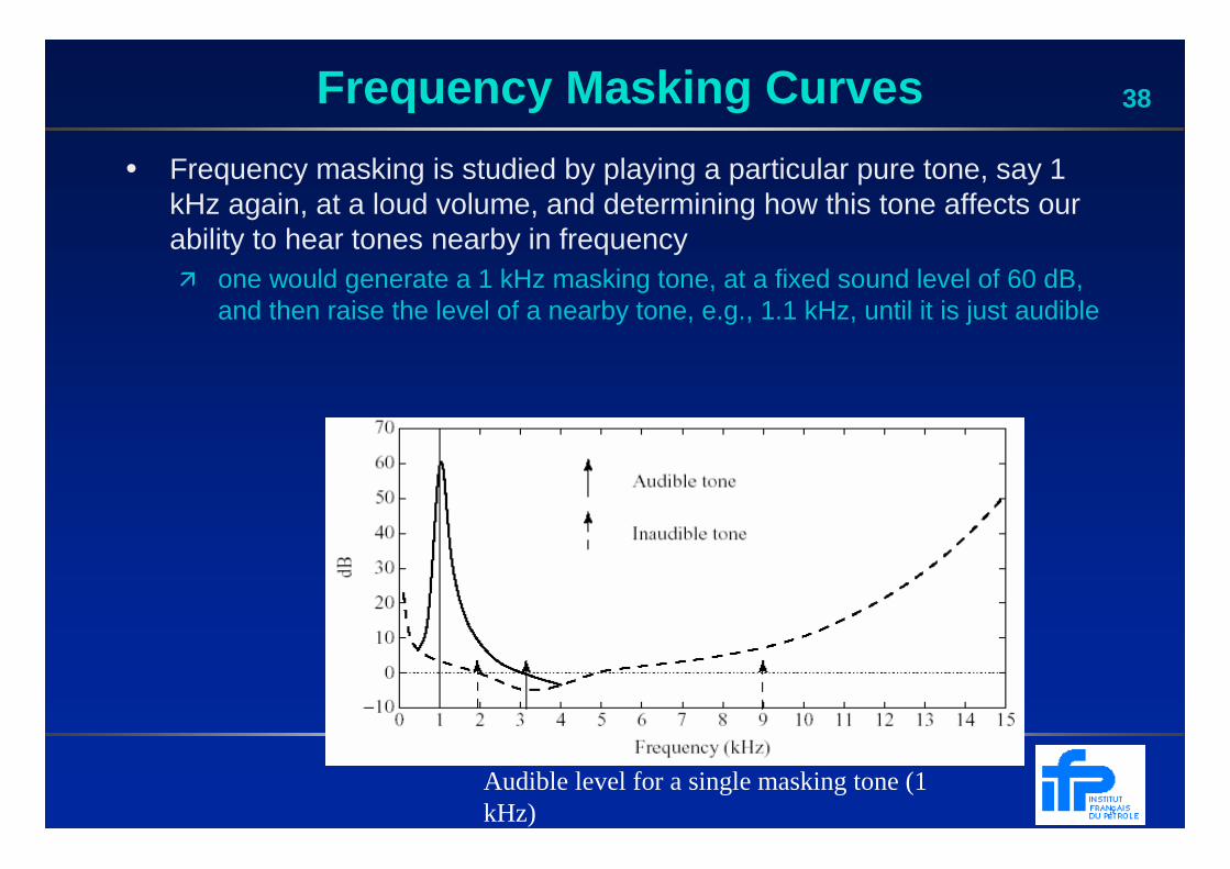
38Frequency Masking Curves

• Frequency masking is studied by playing a particular pure tone, say 1 kHz again, at a loud volume, and determining how this tone affects our ability to hear tones nearby in frequency� one would generate a 1 kHz masking tone, at a fixed sound level of 60 dB,

and then raise the level of a nearby tone, e.g., 1.1 kHz, until it is just audible

Audible level for a single masking tone (1 kHz)

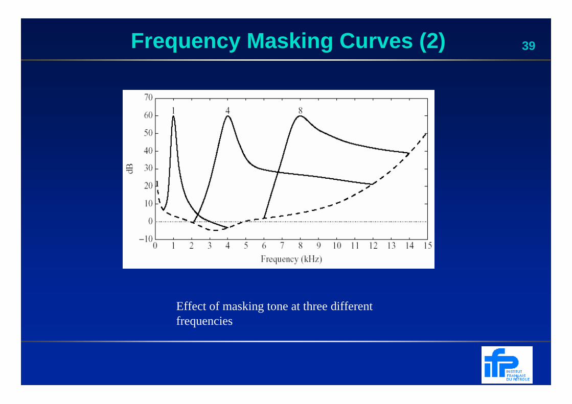
39Frequency Masking Curves (2)

Effect of masking tone at three different frequencies

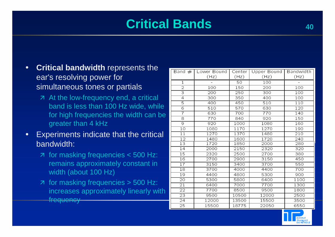
40Critical Bands

• Critical bandwidth represents the ear's resolving power for simultaneous tones or partials� At the low-frequency end, a critical

band is less than 100 Hz wide, while for high frequencies the width can be greater than 4 kHz

• Experiments indicate that the critical bandwidth:� for masking frequencies < 500 Hz:

remains approximately constant in width (about 100 Hz)

� for masking frequencies > 500 Hz: increases approximately linearly with frequency

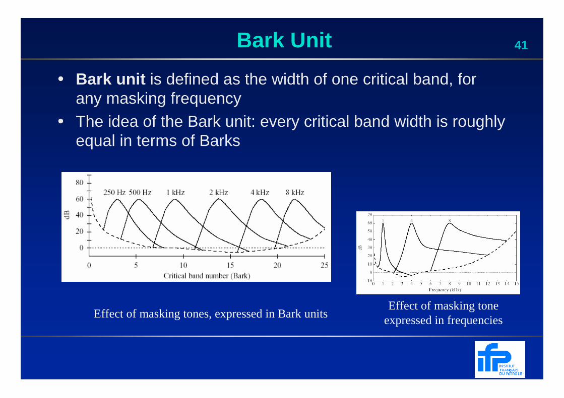
41Bark Unit

• Bark unit is defined as the width of one critical band, for any masking frequency

• The idea of the Bark unit: every critical band width is roughly equal in terms of Barks

Effect of masking tones, expressed in Bark unitsEffect of masking tone

expressed in frequencies

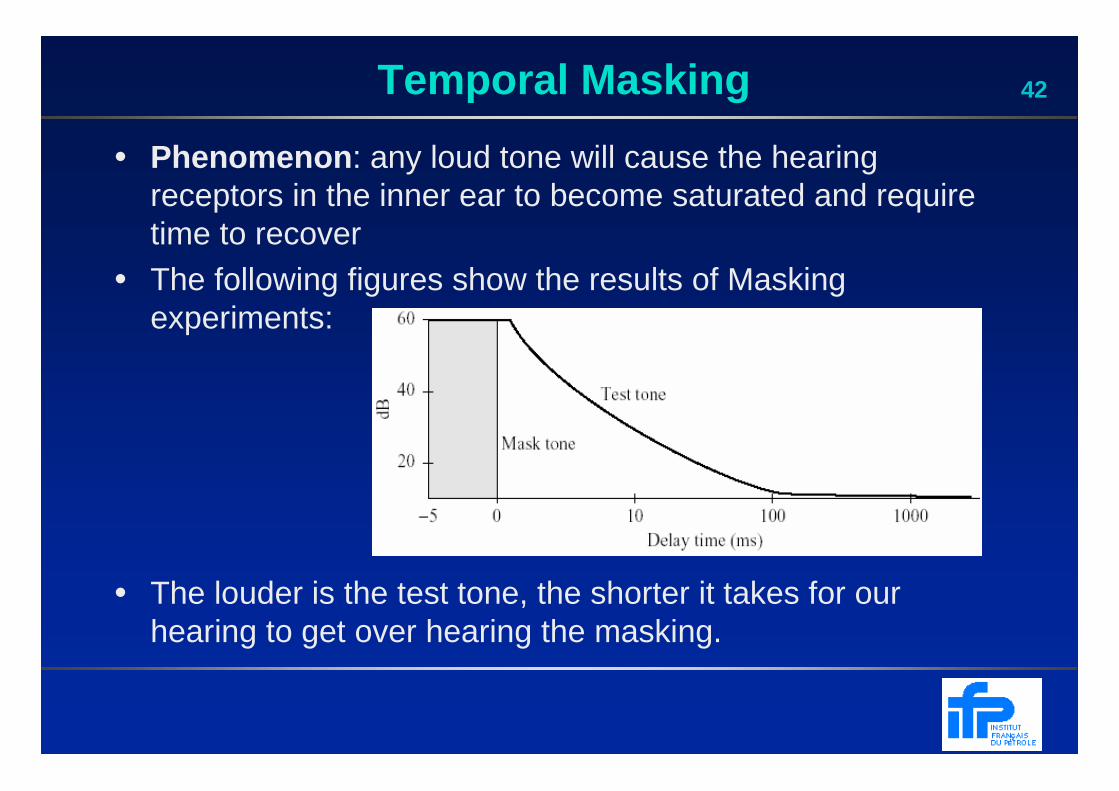
42Temporal Masking

• Phenomenon : any loud tone will cause the hearing receptors in the inner ear to become saturated and require time to recover

• The following figures show the results of Masking experiments:

• The louder is the test tone, the shorter it takes for our hearing to get over hearing the masking.

43Temporal Masking (2)

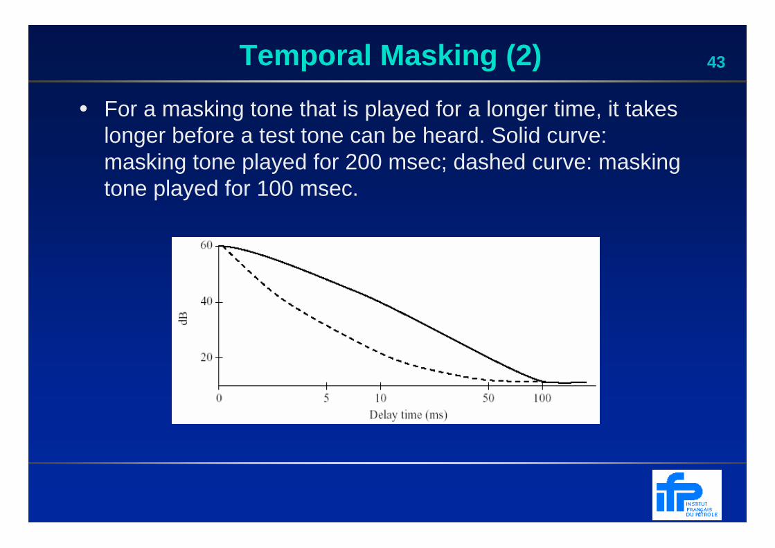
• For a masking tone that is played for a longer time, it takes longer before a test tone can be heard. Solid curve: masking tone played for 200 msec; dashed curve: masking tone played for 100 msec.

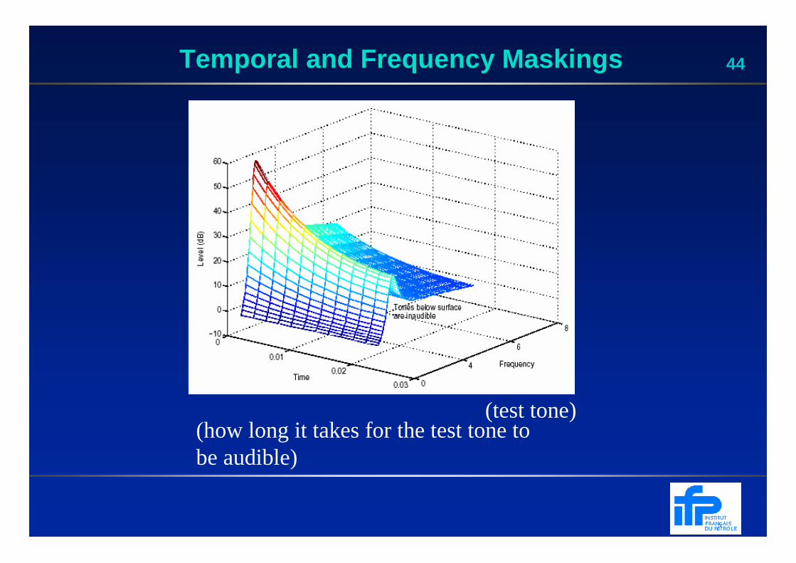
44Temporal and Frequency Maskings

(test tone)(how long it takes for the test tone to be audible)

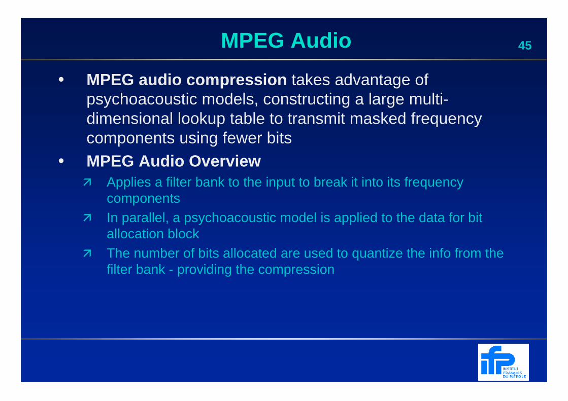
45MPEG Audio

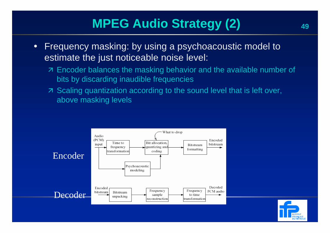
• MPEG audio compression takes advantage of psychoacoustic models, constructing a large multi-dimensional lookup table to transmit masked frequency components using fewer bits

• MPEG Audio Overview� Applies a filter bank to the input to break it into its frequency

components� In parallel, a psychoacoustic model is applied to the data for bit

allocation block� The number of bits allocated are used to quantize the info from the

filter bank - providing the compression

46MPEG-1 Audio Layers

• MPEG-1 audio offers three compatible layers :� Each succeeding layer able to understand the lower layers� Each succeeding layer offering more complexity in the

psychoacoustic model and better compression for a given level ofaudio quality

� Each succeeding layer, with increased compression eeffectiveness, accompanied by extra delay

• The objective of MPEG layers: a good tradeoff between quality and bit-rate

47MPEG-1 Audio Layers (2)

• Layer 1 quality can be quite good provided a comparatively high bit-rate is available� Digital Audio Tape typically uses Layer 1 at around 192 kbps

• Layer 2 has more complexity; was proposed for use in Digital Audio Broadcasting

• Layer 3 (MP3) is most complex, and was originally aimed at audio transmission over ISDN lines

• Most of the complexity increase is at the encoder, not the decoder

48MPEG Audio Strategy

� MPEG approach to compression relies on:– Quantization

– Human auditory system is not accurate within the width of a critical band (perceived loudness and audibility of a frequency)

� MPEG encoder employs a bank of filters to:– Analyze the frequency (“spectral”) components of the audio signal

by calculating a frequency transform of a window of signal values

– Decompose the signal into subbands by using a bank of filters. To keep simplicity, adopts a uniform width for all frequency analysis filters, using 32 overlapping subbands (Recall that audible frequencies are divided into 25 main critical bands with non-uniform bandwidth)

49MPEG Audio Strategy (2)

• Frequency masking: by using a psychoacoustic model to estimate the just noticeable noise level:� Encoder balances the masking behavior and the available number of

bits by discarding inaudible frequencies� Scaling quantization according to the sound level that is left over,

above masking levels

Decoder

Encoder

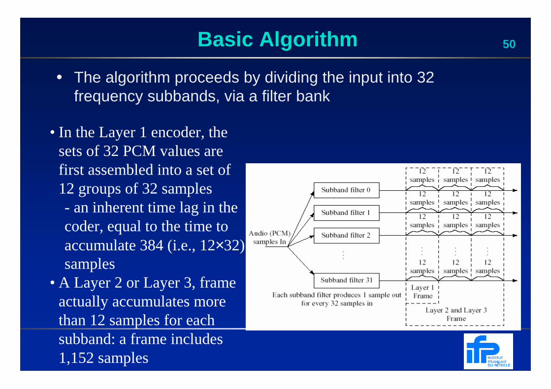
50Basic Algorithm

• The algorithm proceeds by dividing the input into 32 frequency subbands, via a filter bank

• In the Layer 1 encoder, the sets of 32 PCM values are first assembled into a set of 12 groups of 32 samples- an inherent time lag in the coder, equal to the time to accumulate 384 (i.e., 12×32) samples

• A Layer 2 or Layer 3, frame actually accumulates more than 12 samples for each subband: a frame includes 1,152 samples

51

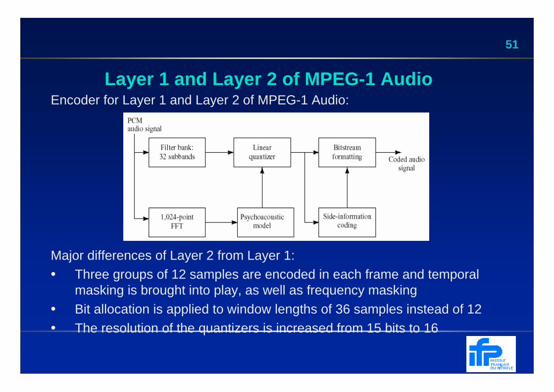
Layer 1 and Layer 2 of MPEG -1 Audio Encoder for Layer 1 and Layer 2 of MPEG-1 Audio:

Major differences of Layer 2 from Layer 1: • Three groups of 12 samples are encoded in each frame and temporal

masking is brought into play, as well as frequency masking• Bit allocation is applied to window lengths of 36 samples instead of 12• The resolution of the quantizers is increased from 15 bits to 16

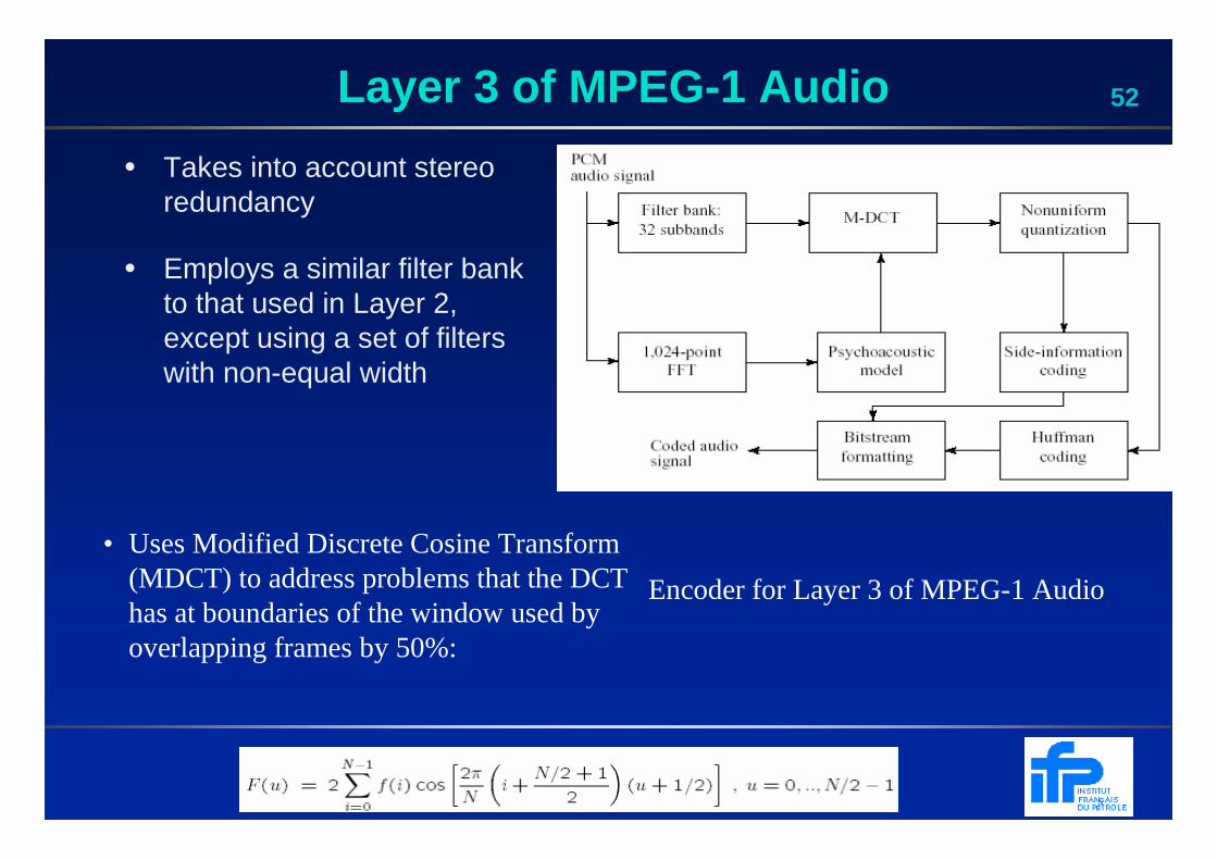
52Layer 3 of MPEG -1 Audio

Encoder for Layer 3 of MPEG-1 Audio

• Takes into account stereo redundancy

• Employs a similar filter bank to that used in Layer 2, except using a set of filters with non-equal width

• Uses Modified Discrete Cosine Transform (MDCT) to address problems that the DCT has at boundaries of the window used by overlapping frames by 50%:

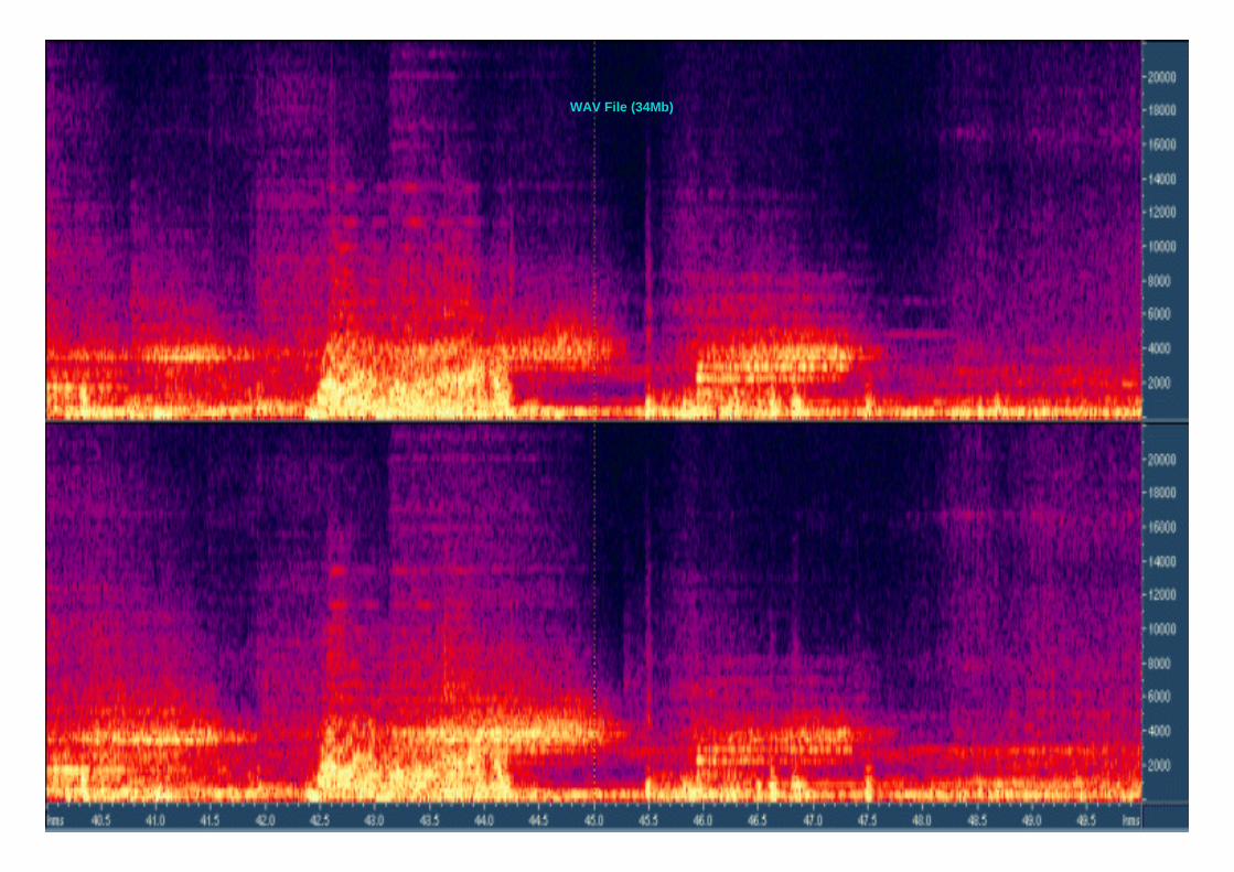
53WAV File (34Mb)

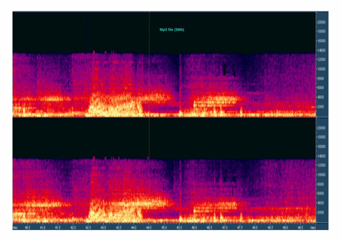
54Mp3 file (3Mb)

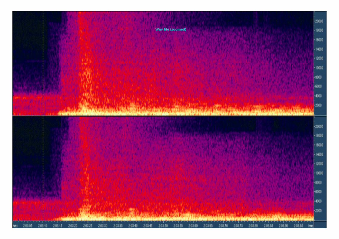
55Wav file (zoomed)

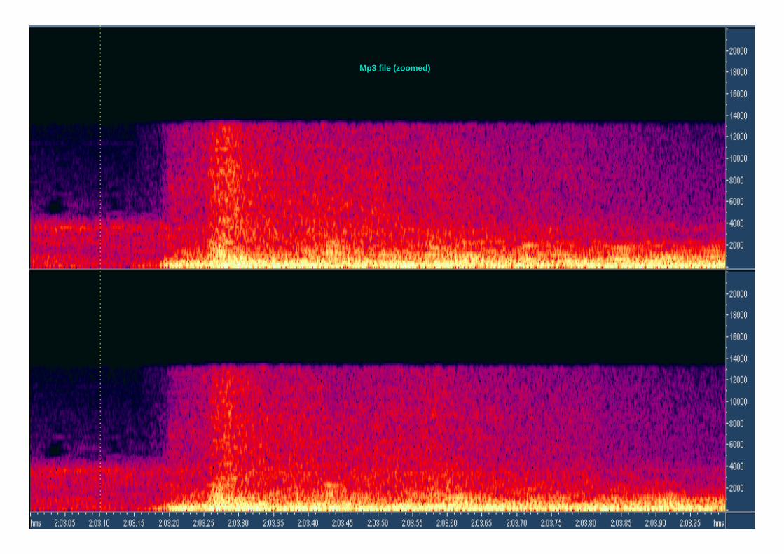
56Mp3 file (zoomed)

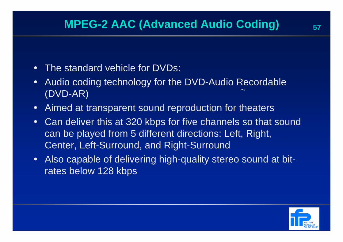
57MPEG-2 AAC (Advanced Audio Coding)

• The standard vehicle for DVDs:• Audio coding technology for the DVD-Audio Recordable

(DVD-AR)• Aimed at transparent sound reproduction for theaters• Can deliver this at 320 kbps for five channels so that sound

can be played from 5 different directions: Left, Right, Center, Left-Surround, and Right-Surround

• Also capable of delivering high-quality stereo sound at bit-rates below 128 kbps

~

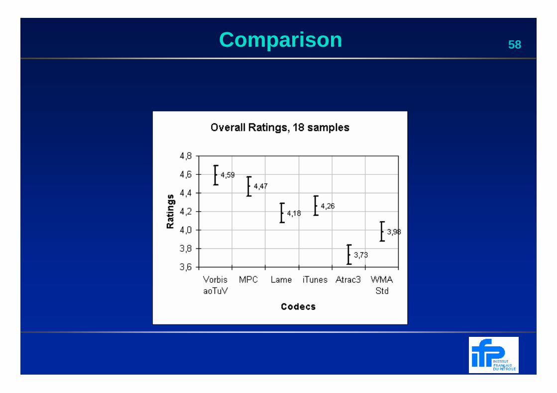
58Comparison

59Existing and Emerging Codecs

• Internet codecs• Multichannel codecs• Lossless codecs• Low delay codecs• New codecs• Others

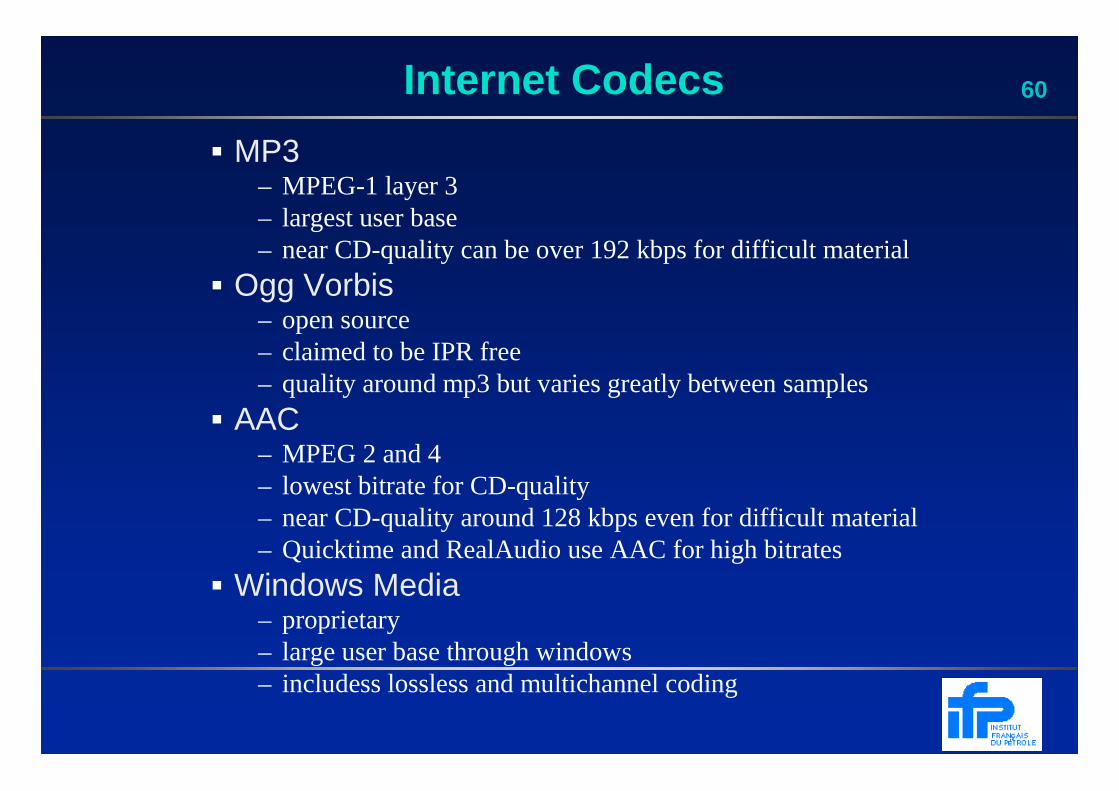
60Internet Codecs

� MP3– MPEG-1 layer 3 – largest user base– near CD-quality can be over 192 kbps for difficult material

� Ogg Vorbis– open source– claimed to be IPR free– quality around mp3 but varies greatly between samples

� AAC– MPEG 2 and 4– lowest bitrate for CD-quality– near CD-quality around 128 kbps even for difficult material– Quicktime and RealAudio use AAC for high bitrates

� Windows Media– proprietary – large user base through windows– includess lossless and multichannel coding

61Internet Codecs Continued

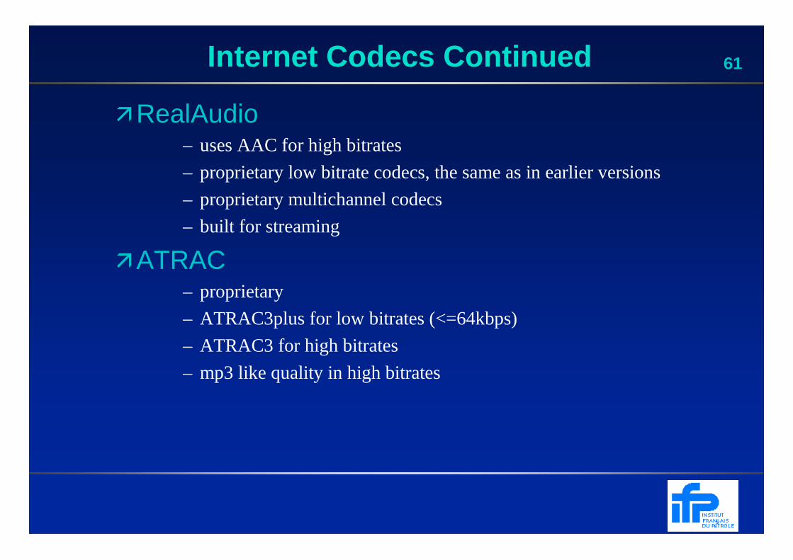
�RealAudio– uses AAC for high bitrates

– proprietary low bitrate codecs, the same as in earlier versions

– proprietary multichannel codecs

– built for streaming

�ATRAC– proprietary

– ATRAC3plus for low bitrates (<=64kbps)

– ATRAC3 for high bitrates

– mp3 like quality in high bitrates

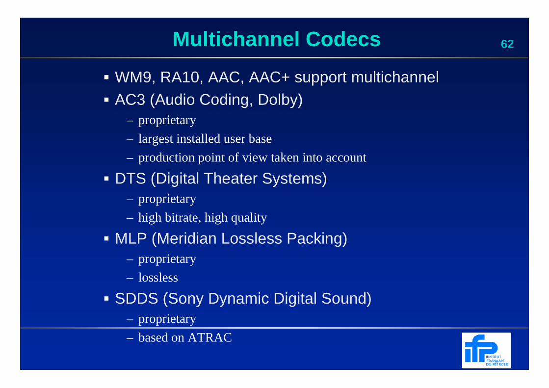
62Multichannel Codecs

� WM9, RA10, AAC, AAC+ support multichannel� AC3 (Audio Coding, Dolby)

– proprietary

– largest installed user base

– production point of view taken into account

� DTS (Digital Theater Systems)– proprietary

– high bitrate, high quality

� MLP (Meridian Lossless Packing)– proprietary

– lossless

� SDDS (Sony Dynamic Digital Sound)– proprietary

– based on ATRAC

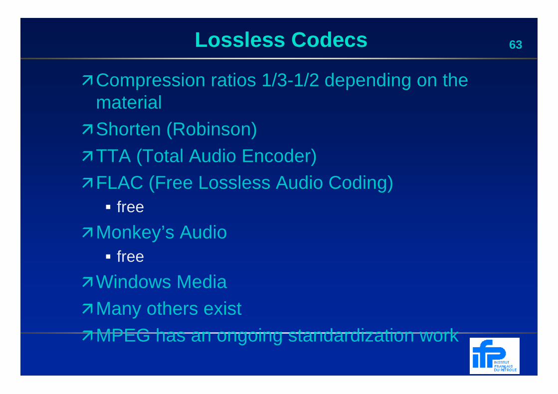
63Lossless Codecs

�Compression ratios 1/3-1/2 depending on the material

�Shorten (Robinson)

�TTA (Total Audio Encoder)�FLAC (Free Lossless Audio Coding)

� free

�Monkey’s Audio� free

�Windows Media�Many others exist

�MPEG has an ongoing standardization work

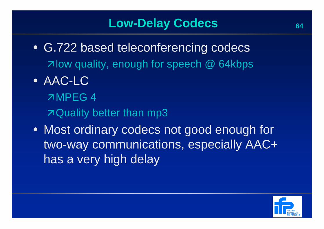
64Low -Delay Codecs

• G.722 based teleconferencing codecs� low quality, enough for speech @ 64kbps

• AAC-LC �MPEG 4

�Quality better than mp3

• Most ordinary codecs not good enough for two-way communications, especially AAC+ has a very high delay

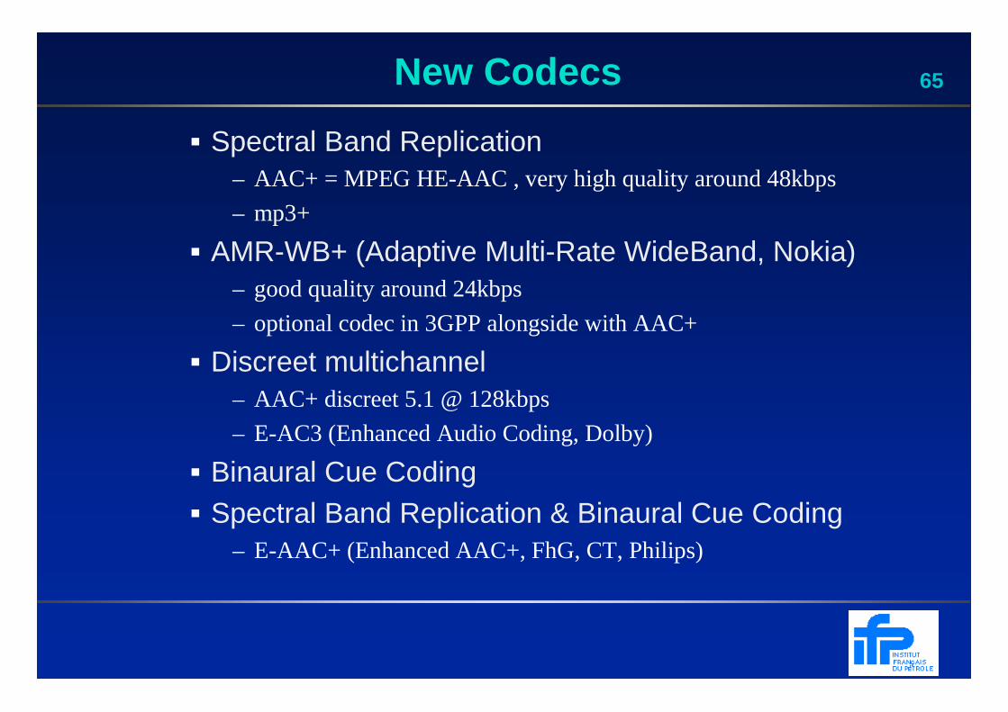
65New Codecs

� Spectral Band Replication– AAC+ = MPEG HE-AAC , very high quality around 48kbps

– mp3+

� AMR-WB+ (Adaptive Multi-Rate WideBand, Nokia)– good quality around 24kbps

– optional codec in 3GPP alongside with AAC+

� Discreet multichannel– AAC+ discreet 5.1 @ 128kbps

– E-AC3 (Enhanced Audio Coding, Dolby)

� Binaural Cue Coding� Spectral Band Replication & Binaural Cue Coding

– E-AAC+ (Enhanced AAC+, FhG, CT, Philips)

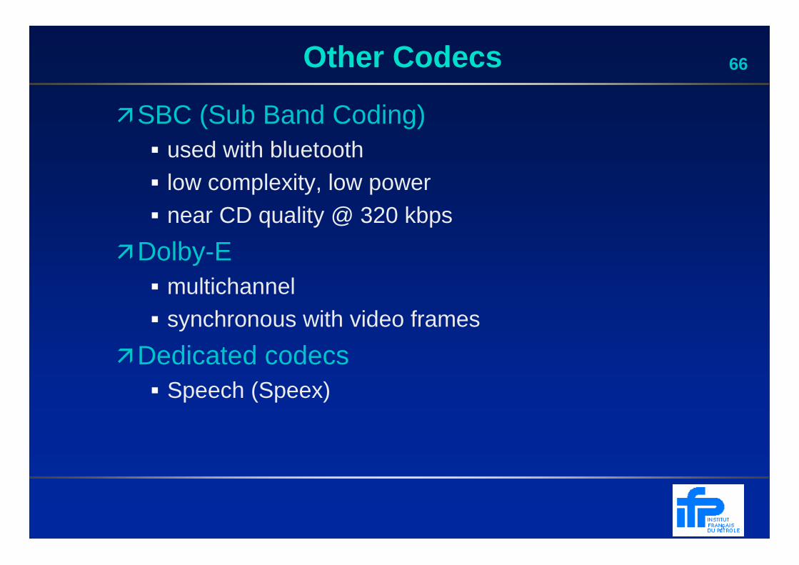
66Other Codecs

�SBC (Sub Band Coding)� used with bluetooth� low complexity, low power� near CD quality @ 320 kbps

�Dolby-E� multichannel� synchronous with video frames

�Dedicated codecs� Speech (Speex)