Embed Size (px)
Citation preview

Lecture 22: Object RecognitionPose

Object recognition• Fundamental ability of a visual system is recognition of
objects– What?– Where?– Who?
• Allows us to interact with the world and classify objects in it
• Goal of computer vision is usually more limited– Prior 2D or 3D model– Find if the model occurs in the image, and where it is– Find what camera position relative to the object would produce
that image

Object Recognition in Living Creatures• Most important aspect of visual perception• Least understood• Young children can recognize large variety of objects
– Child can generalize from a few examples of dogs to many dogs under a variety of visual conditions
• Insects such as bees use visual recognition for navigation and finding its home, identifying flower shapes

Goals of Object Recognition
• Goal is to retrieve information that is not apparent in the images we perceive.
• The name of things is one piece of information• Animals recognize without words. Important
information may be whether to ignore, eat, flee, etc.• A robot could connect the objects it sees to the
information it knows about them, and also connect new information about objects to what it already knows about them.
Three Classes of Recognition Methods
• Alignment methods• Invariant properties methods• Parts decompositions methods
Taxonomy of ideas, not of recognition systems• Systems may combine methods from the 3 classes

Course theme• Computer vision is inference about the world using image
data and prior information• Object recognition is a fundamental part of this• Machine vision
– Assembly line robots – identify machine parts and how they are placed on the assembly line conveyor
• Surveillance and Target finding– Know the shapes of enemy tanks and guns. Find if they are
camouflaged or hidden in satellite or aerial imagery
• Face recognition– Have PONG recognize you

Images• Lots of pixels• Reduce to feature vectors
– Corners– Edges– Filter outputs– Etc.
• Discussed in the first part of the course• Now use these for recognition• Perform feature matching of model image/3D model with
image

Recognizing Objects: Feature Matching
• Problem: Match when viewing conditions change a lot.– Lighting changes: brightness constancy false.– Viewpoint changes: appearance changes, many viewpoints.
• One Solution: Match using edge-based features.– Edges less variable to lighting, viewpoint. – More compact representation can lead to efficiency.
• Match image or object to image– If object, matching may be asymmetric– Object may be 3D.
• Line finding was an example: line=object; points=image.

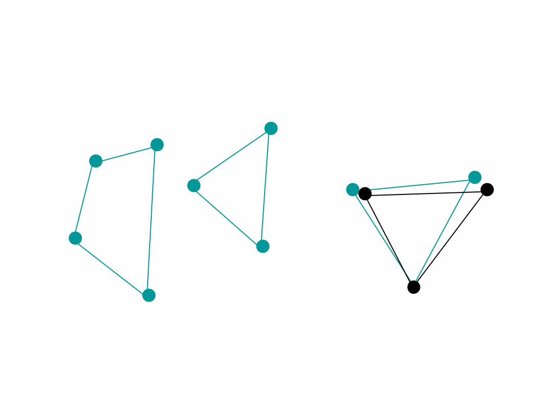
Problem Definition• An Image is a set of 2D geometric features, along with positions.• An Object is a set of 2D/3D geometric features, along with
positions.• A pose positions the object relative to the image.
– 2D Translation; – 2D translation + rotation; – 2D translation, rotation and scale; – planar or 3D object positioned in 3D with perspective or scaled orthographic
projection.• The best pose places the object features nearest the image features

correspondences
3D model2D Image
3D World
zx
y
pose
z
xy

Strategy• Build feature descriptions • Search possible poses.
– Can search space of poses – Or search feature matches (“Correspondence”) , which produce pose
• Transform model by pose.• Compare transformed model and image.• Pick best pose.

Strategy• Already dealt in first part of the course with finding
features.• Now discuss picking best pose since this defines the
problem.• Second discuss search methods appropriate for 2D.• Third discuss transforming model in 2D and 3D.• Fourth discuss search for 3D objects.
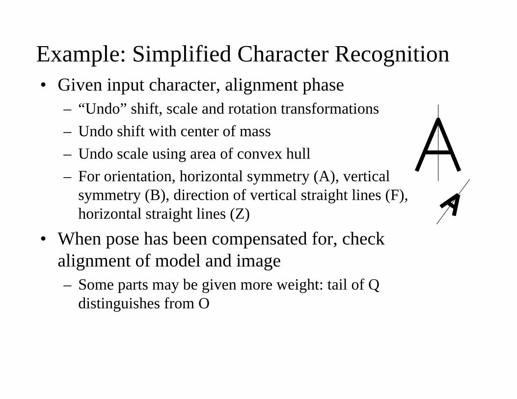
Example: Simplified Character Recognition• Given input character, alignment phase
– “Undo” shift, scale and rotation transformations– Undo shift with center of mass– Undo scale using area of convex hull– For orientation, horizontal symmetry (A), vertical
symmetry (B), direction of vertical straight lines (F), horizontal straight lines (Z)
• When pose has been compensated for, check alignment of model and image– Some parts may be given more weight: tail of Q
distinguishes from O

Evaluate Pose• We look at this first, since it defines the problem.• Again, no perfect measure;
– Trade-offs between veracity of measure and computational considerations.

Chamfer Matching: 2D Model projection to edge matching
∑i
d
For every edge point in the transformed object, compute the distance to the nearest image edge point. Sum distances.
||),||||,,||||,,min(||21 1 mii
n
i iqpqpqp …∑
=

Main Feature:
• Every model point matches an image point.
• An image point can match 0, 1, or more model points.

Variations• Sum a different distance
– f(d) = d2
– or Manhattan distance.– f(d) = 1 if d > threshold, 0 otherwise.
– This is called bounded error.
• Use maximum distance instead of sum.– This is called: directed Hausdorff distance.
• Use other features– Corners.– Lines. Then position and angles of lines must be
similar.• Model line may be subset of image line.

Other “constrained” comparisons• Enforce the constraint that each image feature can match
only one model feature.• Enforce continuity, ordering along curves.• These are more complex to optimize.

Strategy• Discussed finding features.• Discussed problem of picking best pose since this defines
the problem.• Second discuss search methods appropriate for 2D.• Third discuss transforming model in 2D and 3D.• Fourth discuss search for 3D objects.

Pose Search• Simplest approach is to try every pose.• Two problems: many poses, costly to evaluate each.• We can reduce the second problem with:

Chamfer matching
• Given:– binary image, B, of edge and local feature locations – binary “edge template”, T, of shape we want to match
• Let D be an array in registration with B such that D(i,j) is the distance to the nearest “1” in B.– this array is called the distance transform of B
• Goal: Find placement of T in D that minimizes the sum, M, of the distance transform multiplied by the pixel values in T– if T is an exact match to B at location (i,j) then M(i,j) = 0– but if the edges in B are slightly displaced from their ideal
locations in T, we still get a good match using the distance transform technique

Computing the distance transform• Brute force, exact algorithm, is to scan B and find, for
each “0”, its closest “1” using the Euclidean distance.– expensive in time, and difficult to implement
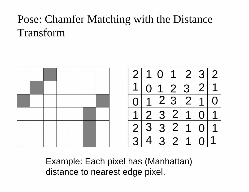
Pose: Chamfer Matching with the Distance Transform
00
0 0000
11
1
11
1
11
1111 1
1
22
22
2222
22
22 33
3333
33 4
Example: Each pixel has (Manhattan) distance to nearest edge pixel.

D.T. Adds Efficiency• Compute once.• Fast algorithms to compute it.• Makes Chamfer Matching simple.

00
0 0000
11
1
11
1
11
1111 1
1
22
22
2222
22
22 33
3333
33 4
Then, try all translations of model edges. Add distances under each edge pixel.

Computing the Distance Transform• It’s only done once, per problem, not once per pose.• Simple solution passing through image once for each distance.
– First pass mark edges 0. – Second, mark 1 anything next to 0, unless it’s already marked. Etc….
• Actually, a more clever method requires 2 passes.

DT Matching example
Pose: Ransac• Match enough features in model to features in image to
determine pose. • Examples:
– match a point and determine translation.– match a corner and determine translation and rotation.– Points and translation, rotation, scaling?– Lines and rotation and translation?

RANSAC• Matching k model and image features determines pose.1. Match k model and image features at Random.2. Determine model pose.3. Project remaining model features into image.4. Count number of model features within ε pixels of an image feature.5. Repeat.6. Pick pose that matches most features.

Issues for RANSAC• How do we determine pose?• How many matches do we need to try?
Presentation Strategy• Already discussed finding features.• First discuss picking best pose since this defines the
problem.• Second discuss search methods appropriate for 2D.• Third discuss transforming model in 2D and 3D.• Fourth discuss search for 3D objects.

Computing Pose: Points• Solve I = S*P.
– In Structure-from-Motion, we knew I.– In Recognition, we know P.
• This is just set of linear equations– Ok, maybe with some non-linear constraints.
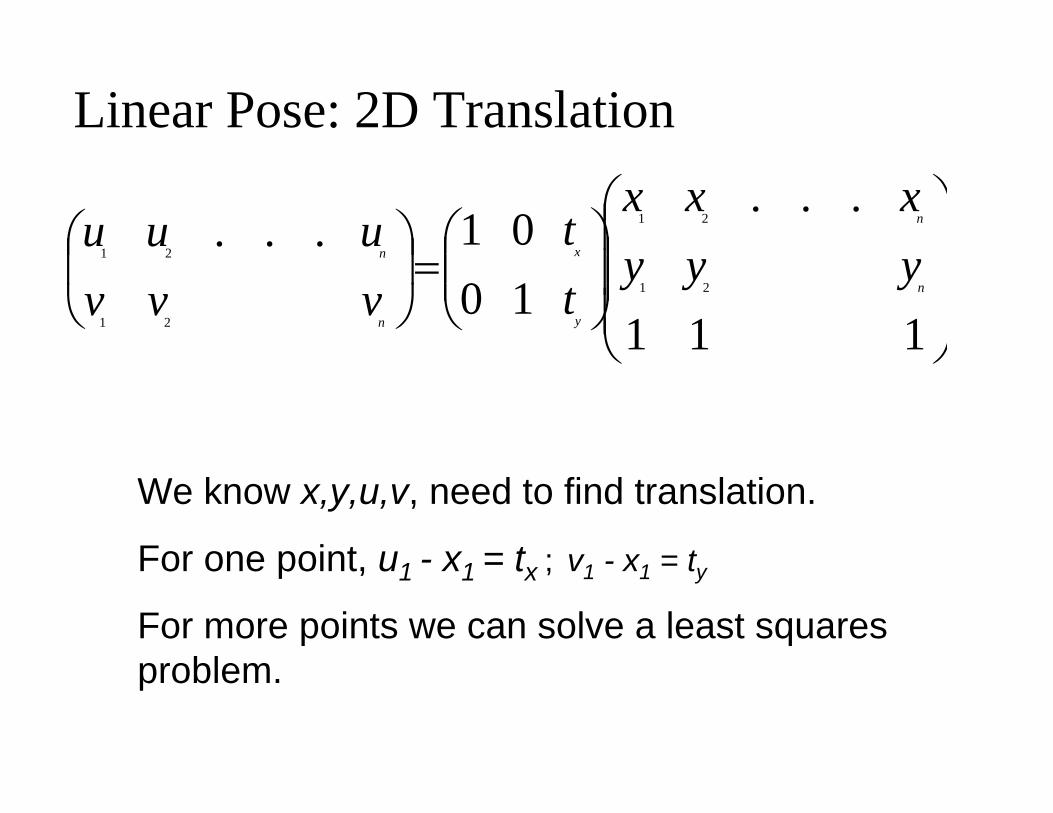
Linear Pose: 2D Translation
⎠
⎞
⎜⎜⎜
⎝
⎛
⎟⎟⎠
⎞⎜⎜⎝
⎛=⎟
⎠
⎞⎜⎝
⎛
111
...
1001...
21
21
21
21
n
n
y
x
n
n yyyxxx
tt
vvvuuu
We know x,y,u,v, need to find translation.
For one point, u1 - x1 = tx ; v1 - x1 = ty
For more points we can solve a least squares problem.

Linear Pose: 2D rotation, translation and scale
θθ
θθθθ
sin,coswith 111
...111
...
cossinsincos...
21
21
21
21
21
21
sbsa
yyyxxx
tabtba
yyyxxx
tt
svvvuuu
n
n
y
x
n
n
y
x
n
n
==
⎟⎟⎟
⎠
⎞
⎜⎜⎜
⎝
⎛
⎟⎟⎠
⎞⎜⎜⎝
⎛−
⎟⎟⎟
⎠
⎞
⎜⎜⎜
⎝
⎛
⎟⎟⎠
⎞⎜⎜⎝
⎛−
=⎟⎠
⎞⎜⎝
⎛
• Notice a and b can take on any values.
• Equations linear in a, b, translation.
• Solve exactly with 2 points, or overconstrained system with more.
sabas =+= θcos22

Linear Pose: 3D Affine
⎟⎟⎟⎟⎟
⎠
⎞
⎜⎜⎜⎜⎜
⎝
⎛
⎟⎟⎠
⎞⎜⎜⎝
⎛=⎟
⎠
⎞⎜⎝
⎛
111
......
21
21
21
3,22,21,2
3,12,11,1
21
21
n
n
n
y
x
n
n
zzzyyyxxx
tssstsss
vvvuuu

Pose: Scaled Orthographic Projection of Planar points
⎟⎟⎟⎟⎟
⎠
⎞
⎜⎜⎜⎜⎜
⎝
⎛
⎟⎟⎠
⎞⎜⎜⎝
⎛=⎟
⎠
⎞⎜⎝
⎛
111000
......
21
21
3,22,21,2
3,12,11,1
21
21 n
n
y
x
n
nyyyxxx
tssstsss
vvvuuu
s1,3, s2,3 disappear. Non-linear constraints disappear with them.

Non-linear pose• A bit trickier. Some results:• 2D rotation and translation. Need 2 points.• 3D scaled orthographic. Need 3 points, give 2 solutions. • 3D perspective, camera known. Need 3 points. Solve 4th
degree polynomial. 4 solutions.

POSIT

Transforming the Object
⎟⎟⎟⎟⎟
⎠
⎞
⎜⎜⎜⎜⎜
⎝
⎛
⎟⎠
⎞⎜⎝
⎛=⎟
⎠
⎞⎜⎝
⎛
111
...
????????
??????
21
21
21
4321
4321
n
n
n
zzzyyyxxx
vvvvuuuu
⎟⎟⎟⎟⎟
⎠
⎞
⎜⎜⎜⎜⎜
⎝
⎛
⎟⎟⎠
⎞⎜⎜⎝
⎛=⎟
⎠
⎞⎜⎝
⎛
111
...
??????
21
21
21
3,22,21,2
3,12,11,1
4321
4321
n
n
n
y
x
zzzyyyxxx
tssstsss
vvvvuuuu
We don’t really want to know pose, we want to know what the object looks like in that pose.
⎟⎟⎟⎟⎟
⎠
⎞
⎜⎜⎜⎜⎜
⎝
⎛
⎟⎟⎠
⎞⎜⎜⎝
⎛=⎟
⎠
⎞⎜⎝
⎛
111
......
21
21
21
3,22,21,2
3,12,11,1
21
21
n
n
n
y
x
n
n
zzzyyyxxx
tssstsss
vvvuuu
We start with:
Solve for pose:
Project rest of points:

Transforming object with Linear Combinations
⎠
⎞
⎜⎜⎜⎜⎜
⎝
⎛
22
2
2
1
22
2
2
1
11
2
1
1
11
2
1
1...
n
n
n
n
vvvuuuvvvuuu
No 3D model, but we’ve seen object twice before.
⎟⎟⎟⎟⎟⎟⎟⎟
⎠
⎞
⎜⎜⎜⎜⎜⎜⎜⎜
⎝
⎛
????
.
.
.
.
3
4
3
3
3
2
3
1
3
4
3
3
3
2
3
1
22
4
2
3
2
2
2
1
21
4
2
3
2
2
2
1
11
4
1
3
1
2
1
1
11
4
1
3
1
2
1
1
vvvvuuuu
vvvvvuuuuuvvvvvuuuuu
n
n
n
n
See four points in third image, need to fill in location of other points.
Just use rank theorem.

Recap: Recognition w/ RANSAC1. Find features in model and image.
– Such as corners.2. Match enough to determine pose.
– Such as 3 points for planar object, scaled orthographic projection.3. Determine pose.4. Project rest of object features into image.5. Look to see how many image features they match.
– Example: with bounded error, count how many object features project near an image feature.
6. Repeat steps 2-5 a bunch of times.7. Pick pose that matches most features.


![オムロン ヘルスケアcff U cff o ÈJt d U/ U 01 St ÈJt s a ÈJt q 011k a.] IINV s (51 S d s s d U S 9-11 U U s s cff s (51 a St s a s s È3t s S](https://img.pdfslide.net/doc/110x75/60da35b7790d9704a70b068a/fff-ff-cff-u-cff-o-jt-d-u-u-01-st-jt-s-a-jt-q-011k.jpg)


![TOWARDS ROBUST LEARNING-BASED POSE ESTIMATION OF ...Space 2016, 2016. [4]S. Sharma and S. D’Amico, \Pose estimation for non-cooperative rendezvous using neural networks," in 2019](https://img.pdfslide.net/doc/110x75/5edf85c5ad6a402d666add15/towards-robust-learning-based-pose-estimation-of-space-2016-2016-4s-sharma.jpg)