Lecture 24 Branch-and-Bound Algorithm - cont.angelia/ge330fall09_bb_nlp_l24.pdf · Branch-and-Bound Algorithm - cont. November 5, ... We branch from the node x3 = 0 since it is a

Lecture 24

Branch-and-Bound Algorithm - cont.

November 5, 2009

Lecture 24

Outline

• Branch-and-Bound Algorithm

• Brief re-cap of the algorithm

• Algorithm demonstrated on an example

• Nonlinear Programming

Operations Research Methods 1

Lecture 24

Initialization

The initial node in the tree corresponds to solving the LP relaxation of the

given problem

LP relaxation is the problem resulting from the given ILP when we “ignore”

integer constraints of the variables

This node is “active” and it is the most recent.


Lecture 24

Typical Iteration for MAXIMIZATION

(a) Branching. Among the most recently created nodes that are “active” select one

(braking ties according to the largest bound). Branch from that node by fixing one of

the “relaxed” variables to 0 and 1 (in the node subproblem)

(b) Bounding. At each new node, solve the corresponding LP problem and determine the

optimal LP value. Round the non-integer value down (to the nearest integer). This is

the bound of the subproblem at the node.

(c) Fathoming. For each new node (subproblem) apply the following three tests:

(1) Integer solution. If one of the new nodes has integer solution, its bound is

compared to the bounds of other such nodes. If it does not have the best value

- it is fathomed. If it has the best value it is fathomed and it is our current best

solution Z∗ (incumbent).

(2) Bound value. If any of the new nodes has a bound smaller than currently the best

bound Z∗ - fathom the node.

(3) Infeasibility. If LP at any of the new nodes has no solution (not feasible) - fathom

the node.


Lecture 24

Termination

Stop when there are no more subproblems (no branching). The node with

the best value provides the solution.

Otherwise perform a new iteration.


Lecture 24

Application

BB algorithm to solve the following ILP:

maximize 9x1 + 5x2 + 6x3 + 4x4

subject to 6x1 + 3x2 + 5x3 + 2x4 ≤ 10

x3 + x4 ≤ 1

−x1 + x3 ≤ 0

−x2 + x4 ≤ 0

xj ∈ {0,1} j = 1, . . . ,4


Lecture 24

Initialization

At the initial node, we would solve its LP relaxation

maximize 9x1 + 5x2 + 6x3 + 4x4

subject to 6x1 + 3x2 + 5x3 + 2x4 ≤ 10

x3 + x4 ≤ 1

−x1 + x3 ≤ 0

−x2 + x4 ≤ 0

0 ≤ xj ≤ 1 j = 1, . . . ,4

Using LP algorithm, we find the optimal value (5/6, 1, 0,1) and the

optimal value z∗ = 1612.

If the solution and the optimal value were integers, we would stop.

Since it is not, this value gives us 16 as the best lower bound on the optimal

value of the ILP (blb = 16).


Lecture 24

The initialization and moving to the first iteration


Lecture 24

Iteration 1:

We branch from the LP relaxation (ALL node) into two new nodes corre-

sponding to x1 = 1 and x1 = 0.

At node x1 = 1 we solve the following LP

maximize 9 + 5x2 + 6x3 + 4x4

subject to 3x2 + 5x3 + 2x4 ≤ 4

x3 + x4 ≤ 1

x3 ≤ 1

−x2 + x4 ≤ 0

0 ≤ xj ≤ 1 j = 2, . . . ,4


Lecture 24

At node x1 = 0 we solve the following LP

maximize 5x2 + 6x3 + 4x4

subject to 3x2 + 5x3 + 2x4 ≤ 10

x3 + x4 ≤ 1

x3 ≤ 0

−x2 + x4 ≤ 0

0 ≤ xj ≤ 1 j = 2, . . . ,4

Node to the right is incumbent and fathomed (no branching there ever).

Node to the left is the only active node and most recent.


Lecture 24

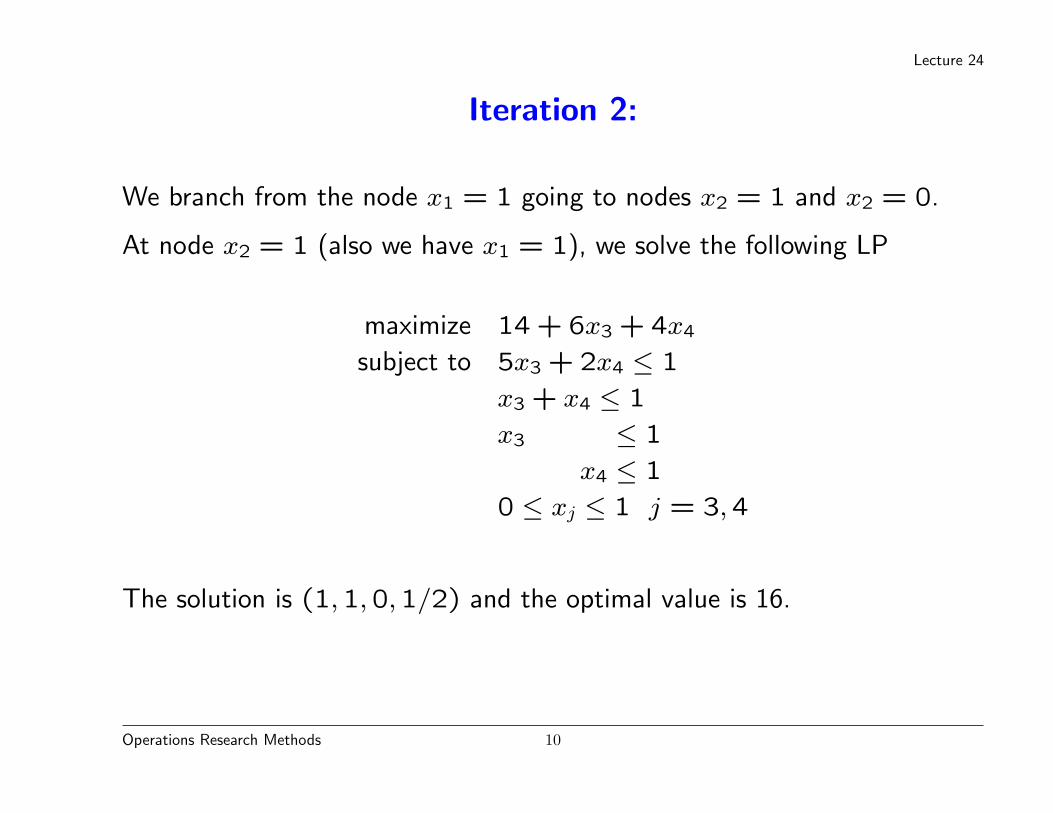
Iteration 2:

We branch from the node x1 = 1 going to nodes x2 = 1 and x2 = 0.

At node x2 = 1 (also we have x1 = 1), we solve the following LP

maximize 14 + 6x3 + 4x4

subject to 5x3 + 2x4 ≤ 1

x3 + x4 ≤ 1

x3 ≤ 1

x4 ≤ 1

0 ≤ xj ≤ 1 j = 3,4

The solution is (1,1,0,1/2) and the optimal value is 16.


Lecture 24

At node x2 = 0 (and x1 = 1) we solve the following LP

maximize 9 + 6x3 + 4x4

subject to 5x3 + 2x4 ≤ 4

x3 + x4 ≤ 1

x3 ≤ 1

x4 ≤ 0

0 ≤ xj ≤ 1 j = 3,4

The solution is (1,0,4/5,0) and the optimal value is 1345.

We round this value down to 13.


Lecture 24

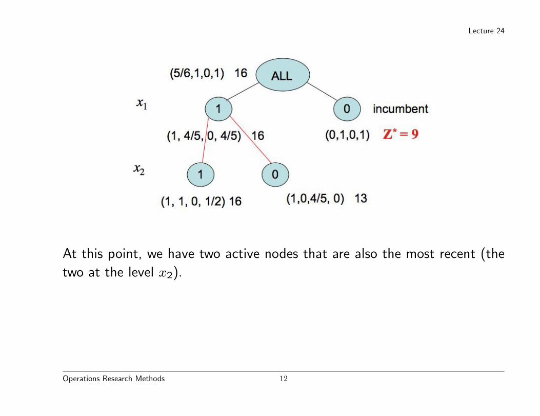
At this point, we have two active nodes that are also the most recent (the

two at the level x2).


Lecture 24

Iteration 3:

We branch from the node x2 = 1 since it has a larger bound of the two

active nodes (16 and 13).

We create two new nodes x3 = 1 and x3 = 0.

At node x3 = 1 (branch x1 = 1 and x2 = 1), we solve the following LP

maximize 20 + 4x4

subject to 2x4 ≤ −4

x4 ≤ 0

x4 ≤ 1

0 ≤ x4 ≤ 1

This LP has no solution - it is infeasible. We fathom this node.


Lecture 24

We now create node x3 = 0 (x1 = 1, x2 = 1).

At this node we solve the following LP

maximize 14 + 4x4

subject to 2x4 ≤ 1

x4 ≤ 1

0 ≤ x4 ≤ 1

The solution is (1,1,0,1/2) and the optimal value is 16.

This node remains active.


Lecture 24

At this point, nodes x2 = 0 and x3 = 0 are active.


Lecture 24

Iteration 4:

We branch from the node x3 = 0 since it is a more recent of the two

remaining active nodes.

We create two new nodes x4 = 1 and x4 = 0.

At node x4 = 1 the problem reduces to: having a point (1,1,0,1) and

the “LP of the form”

maximize 20

subject to 2 ≤ −4

1 ≤ 0

1 ≤ 1

The LP has no solution - it is infeasible. We fathom this node.


Lecture 24

We now create node x4 = 0

At this node we have the following LP

maximize 14

subject to 0 ≤ 1

and the point (1,1,0,0) being feasible. The optimal value is 14.

This node becomes a new incumbent node. A new best value is Z∗ = 14.


Lecture 24

At this point, only the node x2 = 0 is active. Its value is smaller than the current best

Z∗ = 14, so we fathom this node. Since no node is active, the algorithm terminates. The

optimal point and the value are given by the solution and the value at the best incumbent

node, namely (1,1,0,0) and Z∗ = 14.


Lecture 24

Nonlinear Programming


Lecture 24

Nonlinear Programming (NLP) Problems

Characterized by nonlinearities in

• Objective function or

• Constraints

The decision variables are continuous (i.e., take scalar values)

In general, we may have n decision variables x1, . . . , xn.

We often represent these decision variables compactly by a vector x ∈ Rn:

x = (x1, . . . , xn)


Lecture 24

NLP: Formal Model

In general, NLP is the problem of determining a vector x ∈ Rn so as to

maximize f(x)

subject to gi(x) ≤ bi for i = 1, . . . , m

x ∈ X

where f(x) and gi(x) are given functions

f : Rn → R gi : Rn → R,

bi are scalars, and X is a set in Rn. Often, X is the positive orthant

X = {x ∈ Rn | x ≥ 0}

where x ≥ 0 is a compact representation for the relations xi ≥ 0 for all

i = 1, . . . , n.


Lecture 24

Nonlinearity in Objective Function

Typically arises in elastic price model, where the price depends on the

demand


Lecture 24

Example

A company produces two products. The amounts of these products are

denoted by x1 and x2. The production involves 3 different processes

described with the following relations

x1 + 2x2 ≤ 30

3x1 + x2 ≤ 40

x1 + x2 ≥ 10

The costs per unit of production for the products are 2 and 1, respectively.

The selling prices of each of the products is elastic (depends on the demand).

The selling prices of the two products are 2x1 and 3x2 for the amounts x1

and x2, respectively.

The company wants to maximize its profit. Provide the formulation of the

problem.


Lecture 24

The revenue R from selling the amounts x1 and x2 of the products is given

by

R(x1, x2) = (2x1)x1 + (3x2)x2 = 2x21 + 3x2

2

The cost of producing these amounts is

C(x1, x2) = 2x1 + x2

The total profit is

P (x1, x2) = R(x1, x2)− C(x1, x2) = 2x21 + 3x2

2 − 2x1 − x2


Lecture 24

Thus, the problem is

maximize 2x21 + 3x2

2 − 2x1 − x2

x1 + 2x2 ≤ 30

3x1 + x2 ≤ 40

x1 + x2 ≥ 10

x ≥ 0

The objective is nonlinear (in fact quadratic function in x1 and x2)

The constraints are linear


Documents

Lecture 24 Branch-and-Bound Algorithm - cont.angelia/ge330fall09_bb_nlp_l24.pdf · Branch-and-Bound Algorithm - cont. November 5, ... We branch from the node x3 = 0 since it is a