1

1

CIS 467 Image Analysis and Processing

Lecture 25, 05/10/2005

Li ShenComputer and Information Science

UMass Dartmouth

2

Outline

Chapter 1: IntroductionChapter 2: Digital Image FundamentalsChapter 3: Image Enhancement in the Spatial DomainChapter 4: Image Enhancement in the Frequency DomainChapter 5: Image RestorationChapter 7: Wavelets and Multiresolution ProcessingChapter 8: Image CompressionChapter 9: Morphological Image ProcessingChapter 10: Image Segmentation

One page brief notes, calculator

2

3

Chapter 1: Introduction

Source of energy for imagesElectromagnetic (EM) energy spectrumAcoustic, ultrasonic, electronic, synthetic

4

Chapter 2: Fundamentals

Image sensing and acquisitionImage sampling and quantization

Spatial and gray-level resolutionZooming and shrinking

Some basic relationships between pixelsAdjacency, distance, path

Linear and nonlinear operations

3

5

Chapter 3: Image Enhancement in the Spatial Domain

Basic gray level transformationsLinear, logarithmic, power-law

Histogram processingEqualization

Enhancement using arithmetic/logic operationsAveraging, subtraction

Basics of spatial filteringLinearity, near image border

Smoothing spatial filtersAveraging, median

Sharpening spatial filtersLaplacian, Sobel

Point versus mask processing

Smoothing versus sharpening

6

Chapter 4: Image Enhancement in the Frequency Domain

1D Fourier transformDFT, frequency domain, frequency component

2D Fourier transformSpectrum, phase angle, power spectrum, visualization, dc component

Filtering in the frequency domainProcedure, notch filter, lowpass, highpass

Correspondence between filtering in the spatial and frequency domains

Convolution theorem, Gaussian filter

4

7

Chapter 4: Image Enhancement in the Frequency Domain

Smoothing frequency-domain filtersIdeal lowpass filtersButterworth lowpass filtersGaussian lowpass filters

Sharpening frequency-domain filtersIdeal highpass filtersButterworth highpass filtersGaussian highpass filtersHigh-boost filtering

8

Smoothing Filters

SmoothingAttenuating a specified range of high-frequency components in the transform of an image

Three typesIdeal: very sharpButterworth: transition

Parameter: the filter order

Gaussian: very smooth

Ringing behavior

5

9

Sharpening Filters

Reverse operation of lowpass filters

Hhp(u,v) = 1 – Hlp(u,v)

Highpass filtersIdealButterworthGaussian

Unsharp maskingfhp(x,y) = f(x,y)-flp(x,y)

10

Chapter 5: Image Restoration

A model of the image degradation/restoration processNoise modelsRestoration in the presence of noise only-spatial filteringLinear, position-invariant degradationEstimating the degradation functionInverse filteringMinimum mean square error (Wiener) filtering

6

11

Model of Degradation/Restoration

Input: g(x,y), knowledge about H and ηObjective: an estimate of f(x,y)

h: linear, position-invariantg(x,y) = h(x,y) * f(x,y) + η(x,y)G(x,y) = H(u,v) F(u,v) + N(u,v)

12

Noise Models

Histogram and PDFSalt-and-pepper: peak at white endFirst 5 are visually similarEstimate a noise model

7

13

Noise Reduction Using Spatial Filtering

Mean filtersArithmetic and geometricHarmonic and Contra-harmonic

Order-statistics filtersMedian, min, maxAlpha-trimmed filter

Adaptive filtersAdaptive local noise reduction filterAdaptive median filter

14

Adaptive LNR Filters

Zero noise variance, return g(x,y)

g(x,y) = f(x,y)High local variance, return a value similar to g(x,y)

EdgesTwo variances are equal, return arithmetic mean

Noise reduction by averaging

Estimate noise varianceNegative gray levels

22Lσση ≤

8

15

Linear, Position-Invariant Degradations

A linear, spatially-invariant degradation system with additive noise can be modeled in the spatial domain as the convolution of the degradation function with an image, followed by the addition of noise.In the frequency domain, the same process can be expressed as the product of the transforms of the image and degradation, followed by the addition of the transform of the noise.

16

Inverse Filtering

G(u,v)/H(u,v)Apply to the ratioButterworth lowpass function of order 10Cutoff distances 40, 70, 85

9

17

Wiener Filtering

18

Chapter 7: Wavelets and Multi-Resolution Processing

BackgroundImage pyramidsSubband codingThe Haar transform

Multi-resolution expansionsScaling function, wavelets

Wavelet transformsApplications

10

19

Multi-Resolution Expansion

Scaling functionA series of approximationsEach differing by a factor of 2

WaveletsEncode difference between adjacent approximations

20

DWT Application: Edge Detection

11

21

DWT Application: Image Smoothing

22

Chapter 8: Image Compression

FundamentalsCoding redundancyInterpixel redundancyPsychovisual redundancyFidelity Criteria

Image compression modelsThe source encoder and decoderThe channel encoder and decoder

Error-free compressionVariable-length coding

IGS codeRMS errorRMS SNR

12

23

Image Compression Models

Three reduction techniques: combined to form compression systemsOverall characteristics + general modelSource encoder/decoder: remove redundanciesChannel encoder/decoder: increase noise immunity

Hamming Code

Mapper, quantizer, symbol encoder

24

Variable-Length Codes

Arithmetic Coding

Block versus nonblock

13

25

Chapter 9: Morphological Image Processing

PreliminariesSet theory and logic operations

Fundamental operationsDilation and erosionOpening and closingThe hit-or-miss transformation

Some basic morphological algorithmsBoundary extraction, region filling, extraction of connected components, convex hullThinning, thickening, skeletons, pruning

26

Numbers of Components, Holes?

14

27

Chapter 10: Segmentation

Point detectionLine detectionBasic global thresholdingBasic adaptive thresholding

Uneven illumination

28

HW5 Review

15

29

Problem 5.10. Arithmetic and geometric mean filters

Less blurred

Thicker

30

Problem 5.11. Contraharmonic filter

Q>0, pepper noiseQ<0, salt noisePoor result when the wrong polarity is chosen for QQ=-1Any Q, constant gray levels

16

31

Problem 5.26. Telescope images

Telescope images are blurryCannot conduct controlled lab experiments with the lenses and imaging sensorsFormulate a digital image processing solution

32

Problem 7.9. Haar transform

Compute the Haartransform F = [ 3 -1; 6 2]

Inverse Haartransform

17

33

Problem 8.1. Histogram equalized image and compression

Variable-length coding: compress a histogram equalized image

What about interpixel redundancies?

34

Problem 8.4. RMS error and RMS signal-to-noise ratio

RMS error = 14.5

18

35

Problem 8.5. Hamming code

0110: 11001101001: 00110011000: 11100001111: 1111111

1100111: 111, 01101100110: 000, 01101100010: 101, 0110

36

Problem 9.7. Morphological operations

19

37

Project 05-01: Noise generatorfunction im2 =

add_gaussian(im,MU,SIGMA,PROB)

d = size(im);v = rand(d);idx = find(v<PROB); % affect only PROB*100%

pixels

noise = normrnd(MU,SIGMA,d(1),d(2));

im2 = im; im2(idx) = uint8(double(im(idx))+noise(idx));

figure; subplot(1,2,1); imshow(im);subplot(1,2,2); imshow(im2);

function im2 = add_saltpepper(im,PROB1,PROB2)

d = size(im); im2 = im;% PROB1+PROB2 pixels are affectedv = rand(d); idx = find(v<PROB1+PROB2);

% PROB1 pixels are affected by salt noisen = length(idx); v = rand(1,n);ix1 = find(v<PROB1/(PROB1+PROB2)); idx1 =

idx(ix1);im2(idx1) = 255;

% PROB2 pixels are affected by pepper noiseix2 = find(v>=PROB1/(PROB1+PROB2)); idx2 =

idx(ix2);im2(idx2) = 0;

figure; subplot(1,2,1); imshow(im);subplot(1,2,2); imshow(im2);function r = normrnd(mu,sigma,m,n);

r = randn(m,n) .* sigma + mu;

38

Project 05-02: Noise reduction using a median filterim = imread('Fig5.07(a).jpg','jpg');

SALT=0.2; PEPPER=0.2; im2 =

add_saltpepper(im,SALT,PEPPER);

im3 = noisered_med(im2);

function im2 = noisered_med(im)

im2 = medfilt2(im);

figure; subplot(1,2,1); imshow(im);subplot(1,2,2); imshow(im2);

return;

20

39

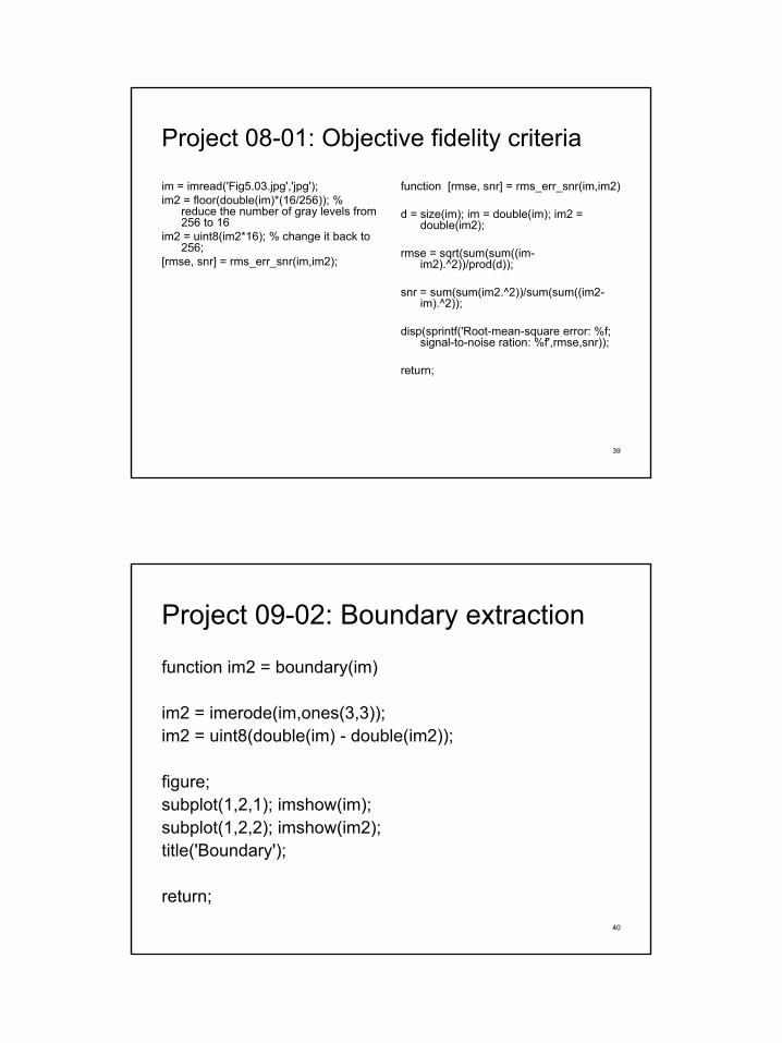
Project 08-01: Objective fidelity criteria

im = imread('Fig5.03.jpg','jpg');im2 = floor(double(im)*(16/256)); %

reduce the number of gray levels from 256 to 16

im2 = uint8(im2*16); % change it back to 256;

[rmse, snr] = rms_err_snr(im,im2);

function [rmse, snr] = rms_err_snr(im,im2)

d = size(im); im = double(im); im2 = double(im2);

rmse = sqrt(sum(sum((im-im2).^2))/prod(d));

snr = sum(sum(im2.^2))/sum(sum((im2-im).^2));

disp(sprintf('Root-mean-square error: %f; signal-to-noise ration: %f',rmse,snr));

return;

40

Project 09-02: Boundary extraction

function im2 = boundary(im)

im2 = imerode(im,ones(3,3));im2 = uint8(double(im) - double(im2));

figure; subplot(1,2,1); imshow(im);subplot(1,2,2); imshow(im2);title('Boundary');

return;

21

41

Project 05-04: Parametric Wiener filter

function pwf(im)

d = size(im);

% create a blurring filterh = fspecial('motion', 50, 50); im2 = imfilter(im, h, 'circular');

% create Gaussian noisem = 0; v = 3; noise = normrnd(m,v,d(1),d(2));im3 = uint8(double(im2) + noise);

% noise-to-power ratiotim = double(im); NSR = sum(noise(:).^2)/sum(tim(:).^2);

% apply wiener filterim4 = deconvwnr(im3,h,NSR);

figure; subplot(2,2,1); imshow(im); title('Original');subplot(2,2,2); imshow(im2); title('Blurred');subplot(2,2,3); imshow(im3); title('Gaussian noise added');subplot(2,2,4); imshow(im4); title('Result');

return;

42

Project 09-04: Morphological solution to Problem 9.27function particles(im)

% make it binaryim1 = zeros(size(im)); idx = find(im>128);

im1(idx) = 1;

% make border to be 1sim1([1 end],:) = 1; im1(:,[1 end]) = 1;

% connected component analysis[L,num] = bwlabel(im1,8);

border = [];overlap = [];nonoverlap = [];

for i=1:numcomp{i} = find(L==i); len(i) = length(comp{i});if len(i)>7000

border = [border; comp{i}];elseif len(i)>400

overlap = [overlap; comp{i}];else

nonoverlap = [nonoverlap; comp{i}];end

End

im2 = zeros(size(im)); im2(border) = 1;im3 = zeros(size(im)); im3(overlap) = 1;im4 = zeros(size(im)); im4(nonoverlap) =

1;

22

43

Thank You

Good luck with the finalsHave a great summer!