Lecture 29 1

More Loop and Nodal Analysis

Lecture 29 2

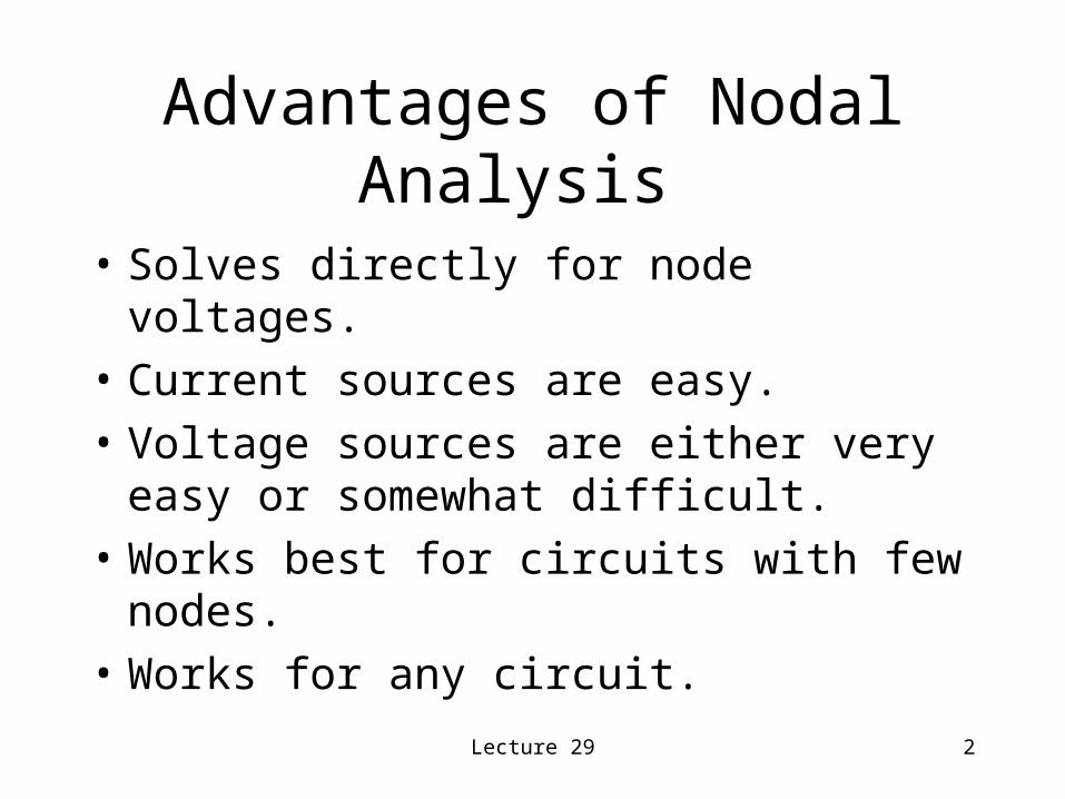
Advantages of Nodal Analysis

• Solves directly for node voltages.

• Current sources are easy.

• Voltage sources are either very easy or somewhat difficult.

• Works best for circuits with few nodes.

• Works for any circuit.

Lecture 29 3

Advantages of Loop Analysis

• Solves directly for some currents.

• Voltage sources are easy.

• Current sources are either very easy or somewhat difficult.

• Works best for circuits with few loops.

Lecture 29 4

Disadvantages of Loop Analysis

• Some currents must be computed from loop currents.

• Does not work with non-planar circuits.

• Choosing the supermesh may be difficult.

Lecture 29 5

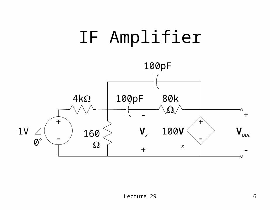
Another Analysis Example

• We will analyze a possible implementation of an AM Radio IF amplifier. (Actually, this would be one of four stages in the IF amplifier.)

• We will solve for output voltages using both nodal and mesh analysis.

• This circuit is a bandpass filter with center frequency 455kHz and bandwidth 40kHz.

Lecture 29 6

IF Amplifier

+

-

4k

+

-1V 0

+

-

Vout

100pF

160

100pF

80k

-

+

Vx 100Vx

Lecture 29 7

Analysis

• Use AC steady state analysis.

• Start with a frequency of =2 455,000.

• Nodal or mesh analysis?

Lecture 29 8

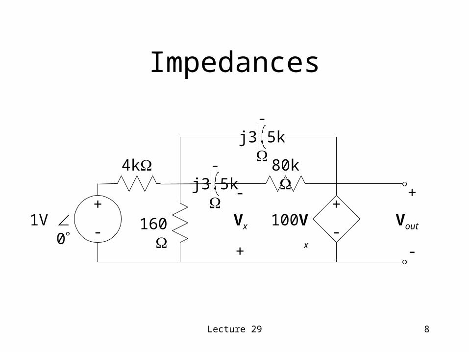
Impedances

+

-

4k

+

-1V 0

+

-

Vout160

80k

-

+

Vx 100Vx

-j3.5k

-j3.5k

Lecture 29 9

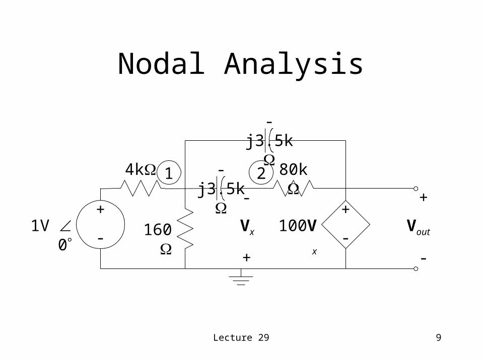
Nodal Analysis

+

-

4k

+

-1V 0

+

-

Vout160

80k

-

+

Vx 100Vx

-j3.5k

-j3.5k1 2

Lecture 29 10

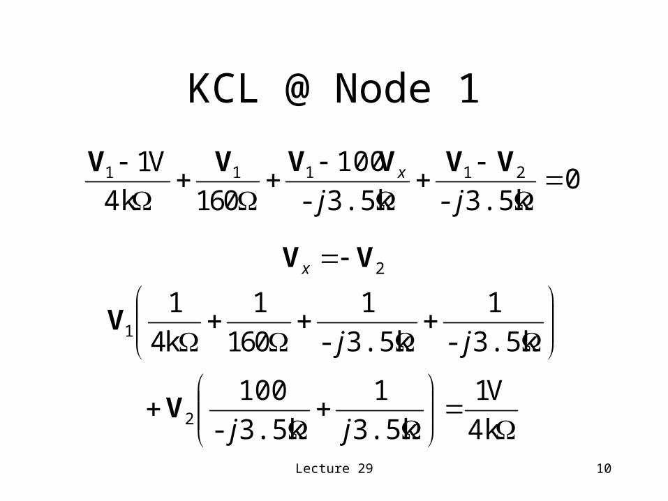
KCL @ Node 1

03.5k-3.5k-

100

0614k

V1 21111

jj

x VVVVVV

4k

V1

3.5k

1

3.5k-

100

3.5k-

1

3.5k-

1

061

1

k4

1

2

1

jj

jj

V

V

2VV x

Lecture 29 11

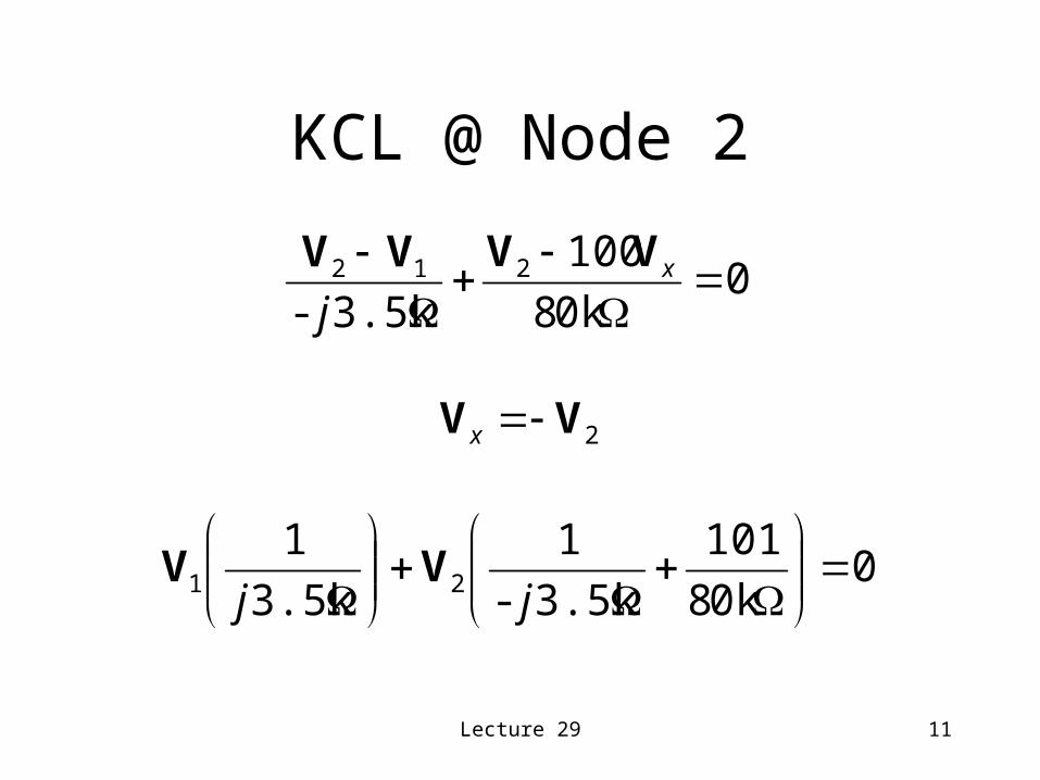
KCL @ Node 2

00k8

100

3.5k-212

x

j

VVVV

00k8

101

3.5k-

1

3.5k

121

jj

VV

2VV x

Lecture 29 12

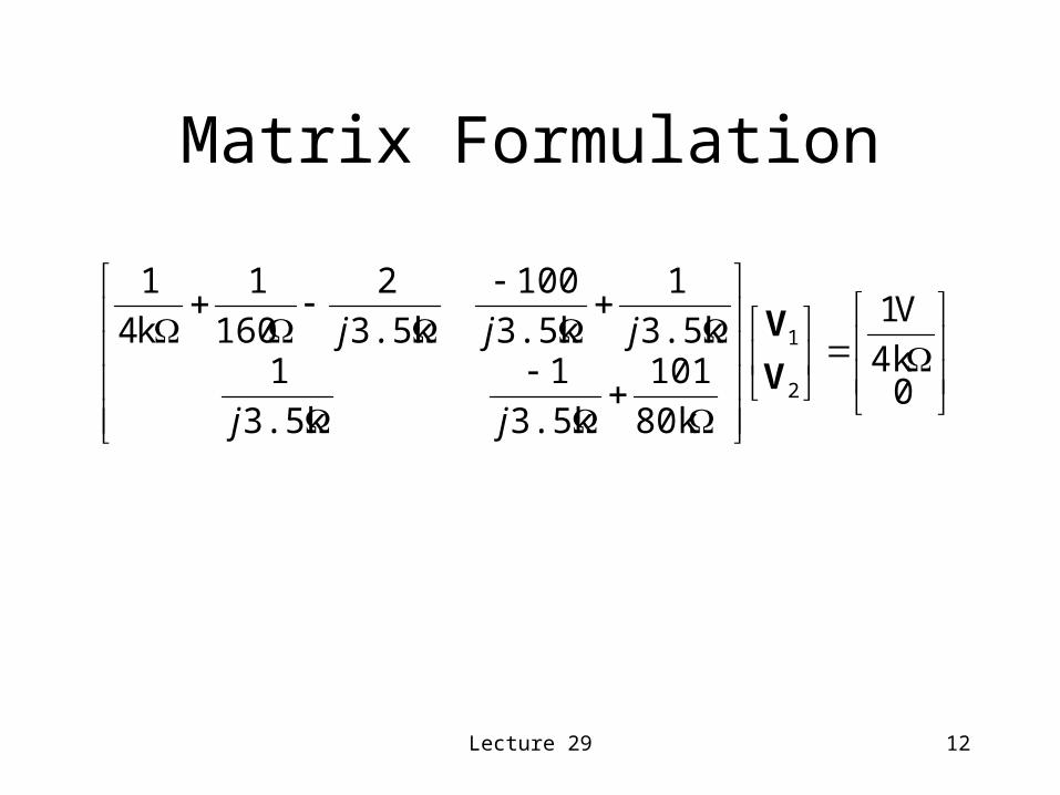
04k

V1

80k

101

3.5k

1

3.5k

13.5k

1

3.5k

100

3.5k

2

160

1

k4

1

2

1

V

V

jj

jjj

Matrix Formulation

Lecture 29 13

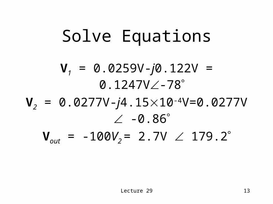
Solve Equations

V1 = 0.0259V-j0.122V = 0.1247V-78

V2 = 0.0277V-j4.1510-4V=0.0277V -0.86

Vout = -100V2 = 2.7V 179.2

Lecture 29 14

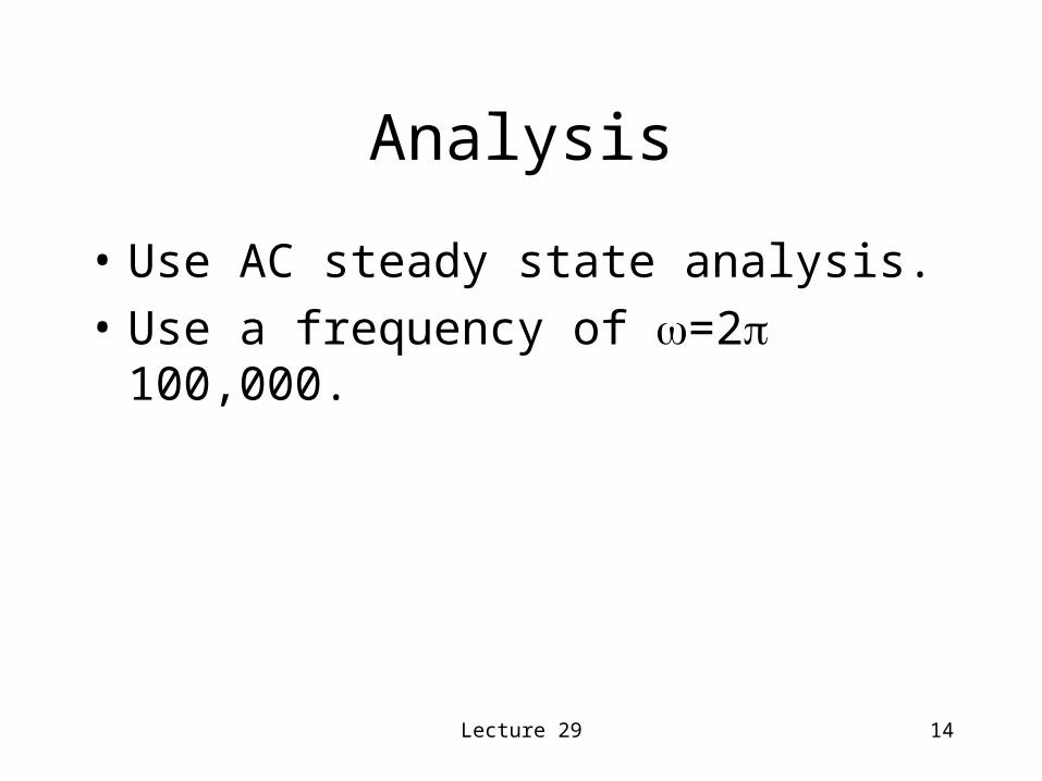
Analysis

• Use AC steady state analysis.

• Use a frequency of =2 100,000.

Lecture 29 15

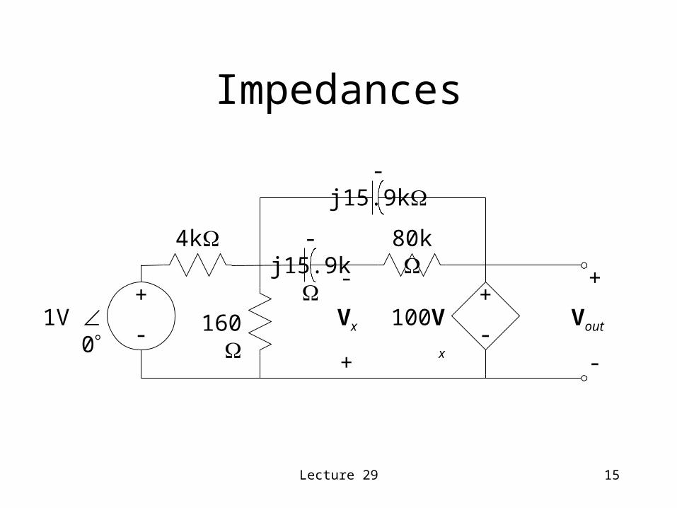
Impedances

+

-

4k

+

-1V 0

+

-

Vout160

80k

-

+

Vx 100Vx

-j15.9k

-j15.9k

Lecture 29 16

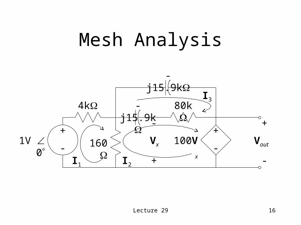
Mesh Analysis

+

-

4k

+

-1V 0

+

-

Vout160

80k

-

+

Vx 100Vx

-j15.9k

-j15.9k

I1 I2

I3

Lecture 29 17

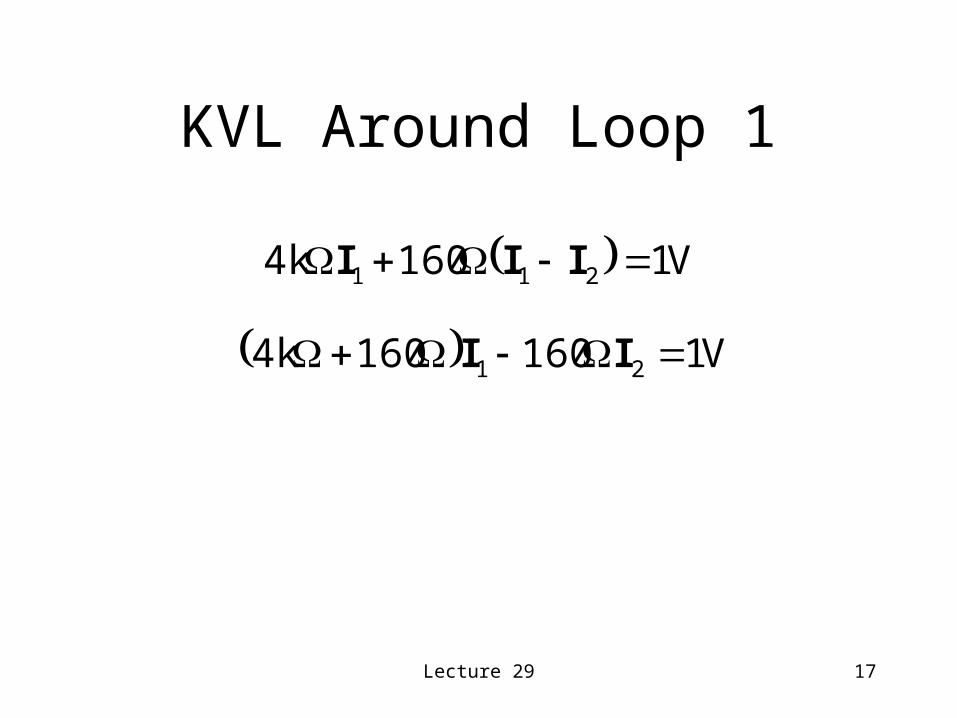
KVL Around Loop 1

V11604k 211 III

V11601604k 21 II

Lecture 29 18

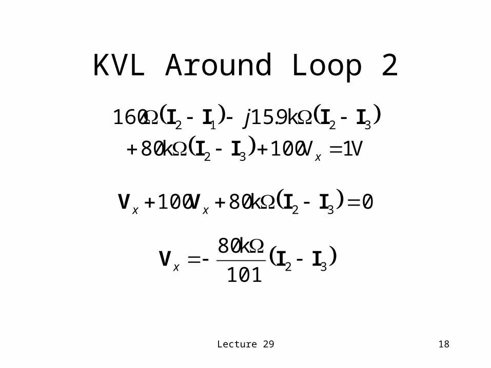
KVL Around Loop 2

V1V100k80

k9.15160

32

3212

x

j

II

IIII

0k80100 32 IIVV xx

32101

k80IIV

x

Lecture 29 19

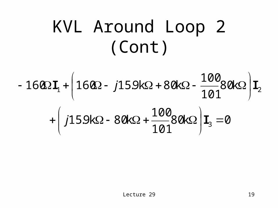
KVL Around Loop 2 (Cont)

0k80101

100k80k9.15

k80101

100k80k9.15160160

3

21

I

II

j

j

Lecture 29 20

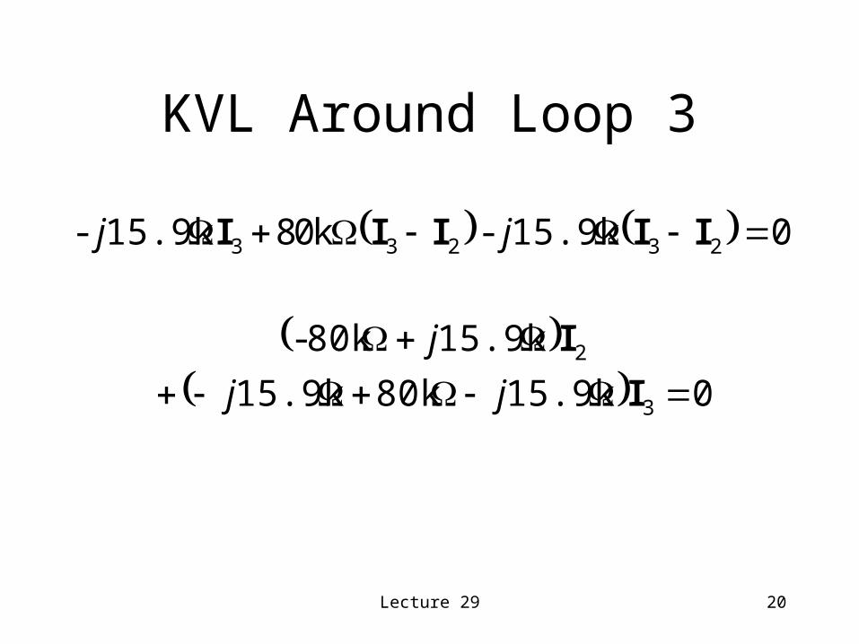
KVL Around Loop 3

015.9k-k0815.9k- 23233 IIIII jj

015.9k80k15.9k

15.9k80k-

3

2

I

I

jj

j

Lecture 29 21

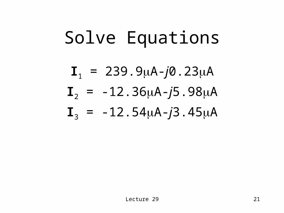
Solve Equations

I1 = 239.9A-j0.23A

I2 = -12.36A-j5.98A

I3 = -12.54A-j3.45A

Lecture 29 22

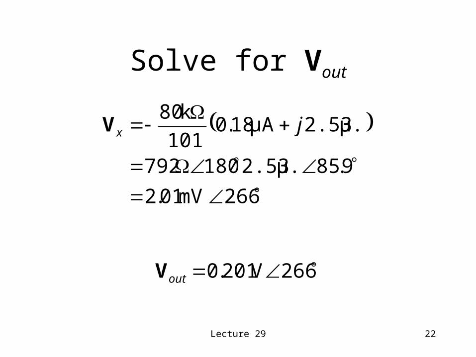
Solve for Vout

266mV01.2

9.852.53μ.180792

2.53μ.μA18.0101

k80jxV

266V201.0outV

Lecture 29 23

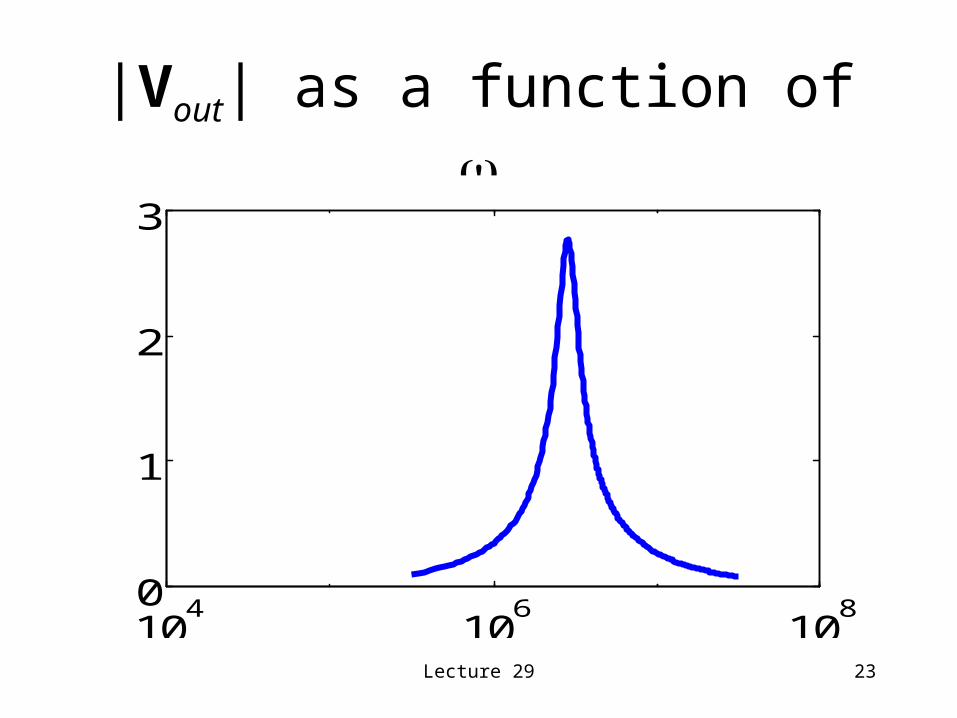
|Vout| as a function of

104

106

108

0

1

2

3