Embed Size (px)
Citation preview
Lecture 3: Bayesian Filtering Equations andKalman Filter
Simo Särkkä
February 10, 2016
Simo Särkkä Lecture 3: Bayesian and Kalman Filtering
Contents
1 Probabilistics State Space Models
2 Bayesian Filter
3 Kalman Filter
4 Examples
5 Summary and Demonstration
Simo Särkkä Lecture 3: Bayesian and Kalman Filtering
Probabilistics State Space Models: General Model
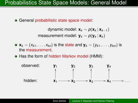
General probabilistic state space model:
dynamic model: xk ∼ p(xk |xk−1)
measurement model: yk ∼ p(yk |xk )
xk = (xk1, . . . , xkn) is the state and yk = (yk1, . . . , ykm) isthe measurement.Has the form of hidden Markov model (HMM):
observed: y1 y2 y3 y4
hidden: x1 //
OO
x2 //
OO
x3 //
OO
x4 //
OO
. . .
Simo Särkkä Lecture 3: Bayesian and Kalman Filtering
Probabilistics State Space Models: Example
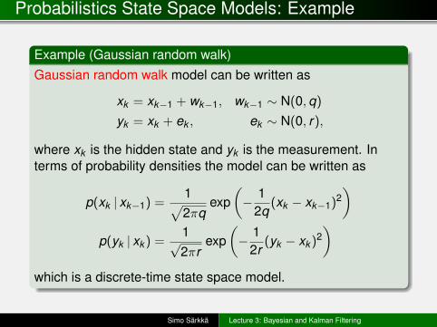
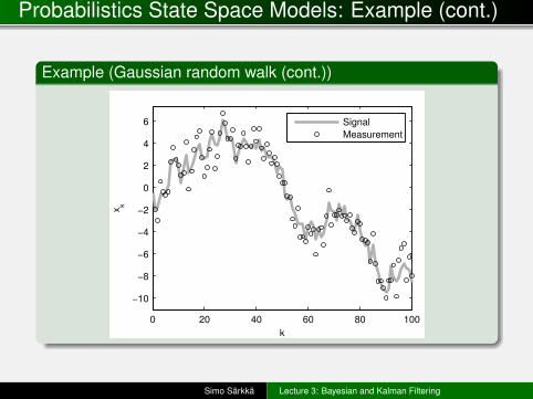
Example (Gaussian random walk)Gaussian random walk model can be written as
xk = xk−1 + wk−1, wk−1 ∼ N(0,q)
yk = xk + ek , ek ∼ N(0, r),
where xk is the hidden state and yk is the measurement. Interms of probability densities the model can be written as
p(xk | xk−1) =1√2πq
exp(− 1
2q(xk − xk−1)2
)p(yk | xk ) =
1√2πr
exp(− 1
2r(yk − xk )2
)which is a discrete-time state space model.
Simo Särkkä Lecture 3: Bayesian and Kalman Filtering
Probabilistics State Space Models: Example (cont.)
Example (Gaussian random walk (cont.))
0 20 40 60 80 100
−10
−8
−6
−4
−2
0
2
4
6
k
xk
Signal
Measurement
Simo Särkkä Lecture 3: Bayesian and Kalman Filtering
Probabilistics State Space Models: Further Examples
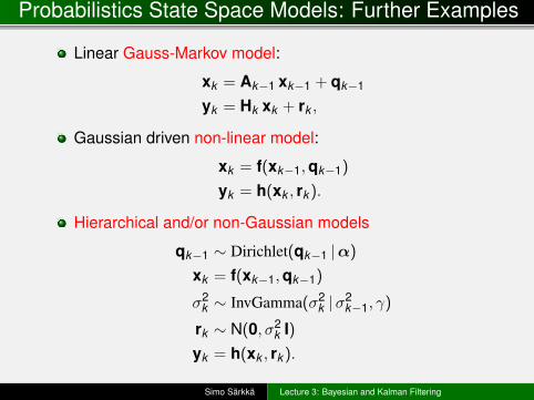
Linear Gauss-Markov model:
xk = Ak−1 xk−1 + qk−1
yk = Hk xk + rk ,
Gaussian driven non-linear model:
xk = f(xk−1,qk−1)
yk = h(xk , rk ).
Hierarchical and/or non-Gaussian models
qk−1 ∼ Dirichlet(qk−1 |α)
xk = f(xk−1,qk−1)
σ2k ∼ InvGamma(σ2
k |σ2k−1, γ)
rk ∼ N(0, σ2k I)
yk = h(xk , rk ).
Simo Särkkä Lecture 3: Bayesian and Kalman Filtering
Probabilistics State Space Models: Markov andIndependence Assumptions
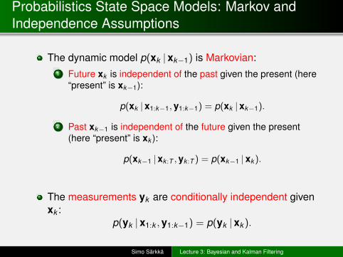
The dynamic model p(xk |xk−1) is Markovian:1 Future xk is independent of the past given the present (here
“present” is xk−1):
p(xk |x1:k−1,y1:k−1) = p(xk |xk−1).
2 Past xk−1 is independent of the future given the present(here “present” is xk ):
p(xk−1 |xk :T ,yk :T ) = p(xk−1 |xk ).
The measurements yk are conditionally independent givenxk :
p(yk |x1:k ,y1:k−1) = p(yk |xk ).
Simo Särkkä Lecture 3: Bayesian and Kalman Filtering
Bayesian Filter: Principle
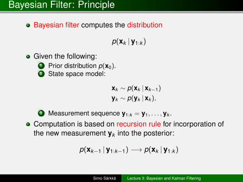
Bayesian filter computes the distribution
p(xk |y1:k )
Given the following:1 Prior distribution p(x0).2 State space model:
xk ∼ p(xk |xk−1)
yk ∼ p(yk |xk ),
3 Measurement sequence y1:k = y1, . . . ,yk .
Computation is based on recursion rule for incorporation ofthe new measurement yk into the posterior:
p(xk−1 |y1:k−1) −→ p(xk |y1:k )
Simo Särkkä Lecture 3: Bayesian and Kalman Filtering
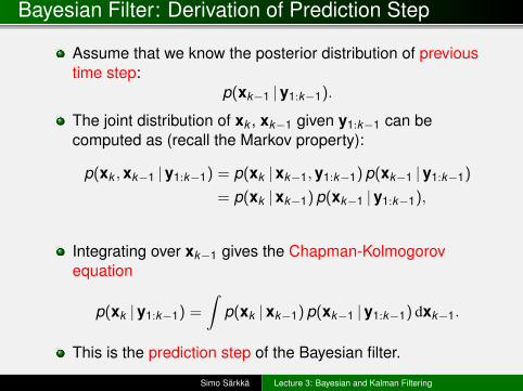
Bayesian Filter: Derivation of Prediction Step
Assume that we know the posterior distribution of previoustime step:
p(xk−1 |y1:k−1).
The joint distribution of xk , xk−1 given y1:k−1 can becomputed as (recall the Markov property):
p(xk ,xk−1 |y1:k−1) = p(xk |xk−1,y1:k−1) p(xk−1 |y1:k−1)
= p(xk |xk−1) p(xk−1 |y1:k−1),
Integrating over xk−1 gives the Chapman-Kolmogorovequation
p(xk |y1:k−1) =
∫p(xk |xk−1) p(xk−1 |y1:k−1) dxk−1.
This is the prediction step of the Bayesian filter.
Simo Särkkä Lecture 3: Bayesian and Kalman Filtering
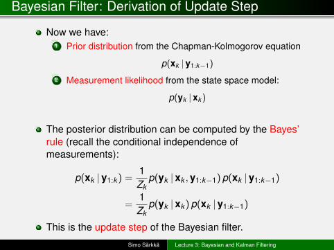
Bayesian Filter: Derivation of Update Step
Now we have:1 Prior distribution from the Chapman-Kolmogorov equation
p(xk |y1:k−1)
2 Measurement likelihood from the state space model:
p(yk |xk )
The posterior distribution can be computed by the Bayes’rule (recall the conditional independence ofmeasurements):
p(xk |y1:k ) =1Zk
p(yk |xk ,y1:k−1) p(xk |y1:k−1)
=1Zk
p(yk |xk ) p(xk |y1:k−1)
This is the update step of the Bayesian filter.
Simo Särkkä Lecture 3: Bayesian and Kalman Filtering
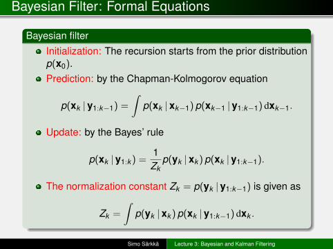
Bayesian Filter: Formal Equations
Bayesian filterInitialization: The recursion starts from the prior distributionp(x0).Prediction: by the Chapman-Kolmogorov equation
p(xk |y1:k−1) =
∫p(xk |xk−1) p(xk−1 |y1:k−1) dxk−1.
Update: by the Bayes’ rule
p(xk |y1:k ) =1Zk
p(yk |xk ) p(xk |y1:k−1).
The normalization constant Zk = p(yk |y1:k−1) is given as
Zk =
∫p(yk |xk ) p(xk |y1:k−1) dxk .
Simo Särkkä Lecture 3: Bayesian and Kalman Filtering
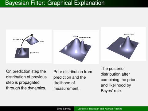
Bayesian Filter: Graphical Explanation
On prediction step thedistribution of previousstep is propagatedthrough the dynamics.
Prior distribution fromprediction and thelikelihood ofmeasurement.
The posteriordistribution aftercombining the priorand likelihood byBayes’ rule.
Simo Särkkä Lecture 3: Bayesian and Kalman Filtering
Kalman Filter: Model
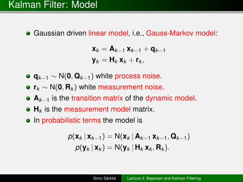
Gaussian driven linear model, i.e., Gauss-Markov model:
xk = Ak−1 xk−1 + qk−1
yk = Hk xk + rk ,
qk−1 ∼ N(0,Qk−1) white process noise.rk ∼ N(0,Rk ) white measurement noise.Ak−1 is the transition matrix of the dynamic model.Hk is the measurement model matrix.In probabilistic terms the model is
p(xk |xk−1) = N(xk |Ak−1 xk−1,Qk−1)
p(yk |xk ) = N(yk |Hk xk ,Rk ).
Simo Särkkä Lecture 3: Bayesian and Kalman Filtering
Kalman Filter: Derivation Preliminaries
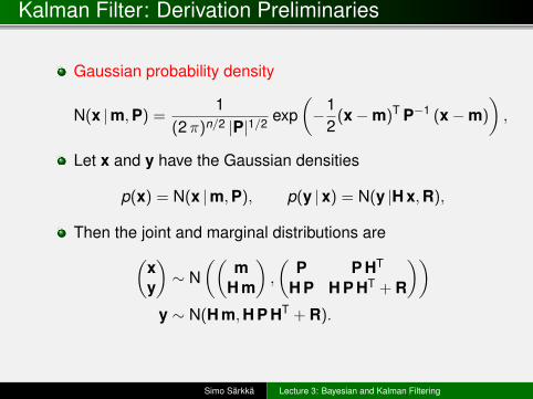
Gaussian probability density
N(x |m,P) =1
(2π)n/2 |P|1/2 exp(−1
2(x−m)T P−1 (x−m)
),
Let x and y have the Gaussian densities
p(x) = N(x |m,P), p(y |x) = N(y |H x,R),
Then the joint and marginal distributions are(xy
)∼ N
((m
H m
),
(P P HT
H P H P HT + R
))y ∼ N(H m,H P HT + R).
Simo Särkkä Lecture 3: Bayesian and Kalman Filtering
Kalman Filter: Derivation Preliminaries (cont.)
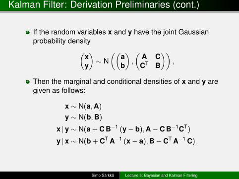
If the random variables x and y have the joint Gaussianprobability density(
xy
)∼ N
((ab
),
(A CCT B
)),
Then the marginal and conditional densities of x and y aregiven as follows:
x ∼ N(a,A)
y ∼ N(b,B)
x |y ∼ N(a + C B−1 (y− b),A− C B−1CT)
y |x ∼ N(b + CT A−1 (x− a),B− CT A−1 C).
Simo Särkkä Lecture 3: Bayesian and Kalman Filtering
Kalman Filter: Derivation of Prediction Step
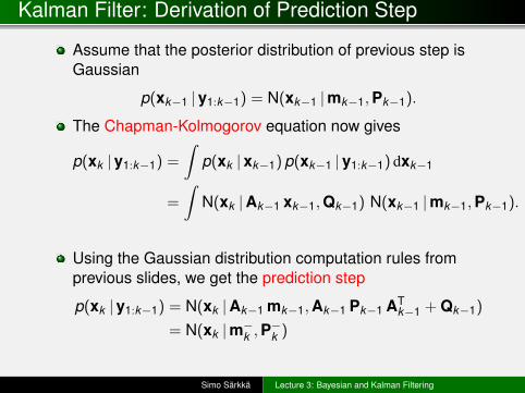
Assume that the posterior distribution of previous step isGaussian
p(xk−1 |y1:k−1) = N(xk−1 |mk−1,Pk−1).
The Chapman-Kolmogorov equation now gives
p(xk |y1:k−1) =
∫p(xk |xk−1) p(xk−1 |y1:k−1) dxk−1
=
∫N(xk |Ak−1 xk−1,Qk−1) N(xk−1 |mk−1,Pk−1).
Using the Gaussian distribution computation rules fromprevious slides, we get the prediction step
p(xk |y1:k−1) = N(xk |Ak−1 mk−1,Ak−1 Pk−1 ATk−1 + Qk−1)
= N(xk |m−k ,P−k )
Simo Särkkä Lecture 3: Bayesian and Kalman Filtering
Kalman Filter: Derivation of Update Step
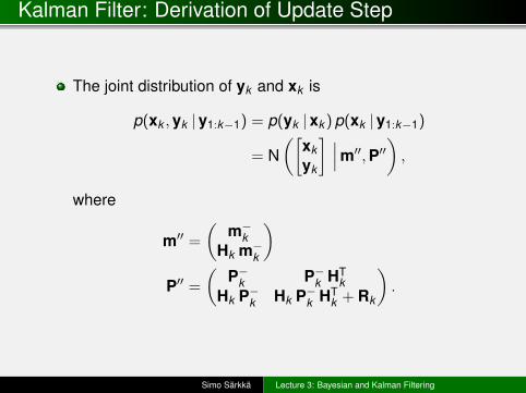
The joint distribution of yk and xk is
p(xk ,yk |y1:k−1) = p(yk |xk ) p(xk |y1:k−1)
= N([
xkyk
] ∣∣∣m′′,P′′) ,where
m′′ =
(m−k
Hk m−k
)P′′ =
(P−k P−k HT
kHk P−k Hk P−k HT
k + Rk
).
Simo Särkkä Lecture 3: Bayesian and Kalman Filtering
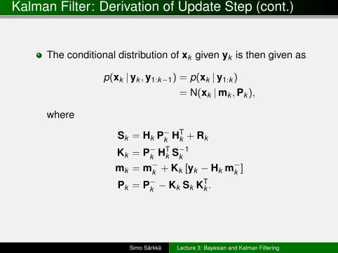
Kalman Filter: Derivation of Update Step (cont.)
The conditional distribution of xk given yk is then given as
p(xk |yk ,y1:k−1) = p(xk |y1:k )
= N(xk |mk ,Pk ),
where
Sk = Hk P−k HTk + Rk
Kk = P−k HTk S−1
k
mk = m−k + Kk [yk − Hk m−k ]
Pk = P−k − Kk Sk KTk .
Simo Särkkä Lecture 3: Bayesian and Kalman Filtering
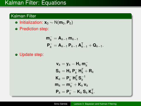
Kalman Filter: Equations
Kalman FilterInitialization: x0 ∼ N(m0,P0)
Prediction step:
m−k = Ak−1 mk−1
P−k = Ak−1 Pk−1 ATk−1 + Qk−1.
Update step:
vk = yk − Hk m−kSk = Hk P−k HT
k + Rk
Kk = P−k HTk S−1
k
mk = m−k + Kk vk
Pk = P−k − Kk Sk KTk .
Simo Särkkä Lecture 3: Bayesian and Kalman Filtering
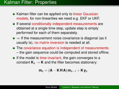
Kalman Filter: Properties
Kalman filter can be applied only to linear Gaussianmodels, for non-linearities we need e.g. EKF or UKF.If several conditionally independent measurements areobtained at a single time step, update step is simplyperformed for each of them separately.⇒ If the measurement noise covariance is diagonal (as itusually is), no matrix inversion is needed at all.The covariance equation is independent of measurements– the gain sequence could be computed and stored offline.If the model is time-invariant, the gain converges to aconstant Kk → K and the filter becomes stationary:
mk = (A− K H A) mk−1 + K yk
Simo Särkkä Lecture 3: Bayesian and Kalman Filtering
Kalman Filter: Random Walk Example
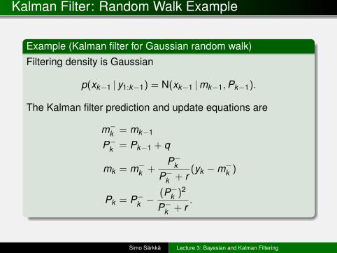
Example (Kalman filter for Gaussian random walk)Filtering density is Gaussian
p(xk−1 | y1:k−1) = N(xk−1 |mk−1,Pk−1).
The Kalman filter prediction and update equations are
m−k = mk−1
P−k = Pk−1 + q
mk = m−k +P−k
P−k + r(yk −m−k )
Pk = P−k −(P−k )2
P−k + r.
Simo Särkkä Lecture 3: Bayesian and Kalman Filtering
Kalman Filter: Random Walk Example (cont.)
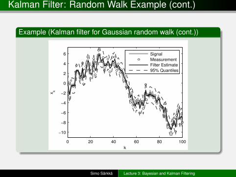
Example (Kalman filter for Gaussian random walk (cont.))
0 20 40 60 80 100
−10
−8
−6
−4
−2
0
2
4
6
k
xk
Signal
Measurement
Filter Estimate
95% Quantiles
Simo Särkkä Lecture 3: Bayesian and Kalman Filtering
Kalman Filter: Car Tracking Example [1/4]
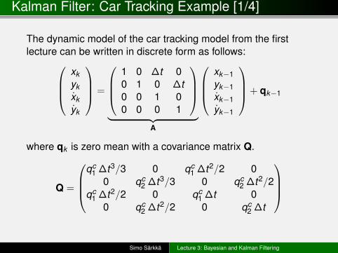
The dynamic model of the car tracking model from the firstlecture can be written in discrete form as follows:
xkykxkyk
=
1 0 ∆t 00 1 0 ∆t0 0 1 00 0 0 1
︸ ︷︷ ︸
A
xk−1yk−1xk−1yk−1
+ qk−1
where qk is zero mean with a covariance matrix Q.
Q =
qc
1 ∆t3/3 0 qc1 ∆t2/2 0
0 qc2 ∆t3/3 0 qc
2 ∆t2/2qc
1 ∆t2/2 0 qc1 ∆t 0
0 qc2 ∆t2/2 0 qc
2 ∆t
Simo Särkkä Lecture 3: Bayesian and Kalman Filtering
Kalman Filter: Car Tracking Example [2/4]
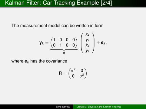
The measurement model can be written in form
yk =
(1 0 0 00 1 0 0
)︸ ︷︷ ︸
H
xkykxkyk
+ ek ,
where ek has the covariance
R =
(σ2 00 σ2
)
Simo Särkkä Lecture 3: Bayesian and Kalman Filtering
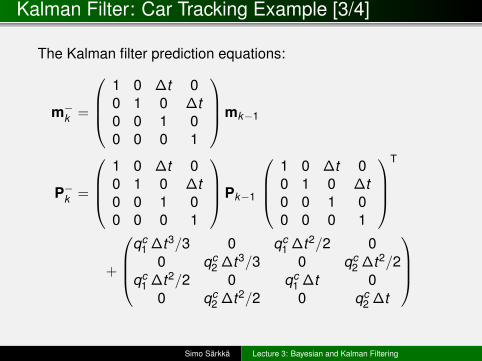
Kalman Filter: Car Tracking Example [3/4]
The Kalman filter prediction equations:
m−k =
1 0 ∆t 00 1 0 ∆t0 0 1 00 0 0 1
mk−1
P−k =
1 0 ∆t 00 1 0 ∆t0 0 1 00 0 0 1
Pk−1
1 0 ∆t 00 1 0 ∆t0 0 1 00 0 0 1
T
+
qc
1 ∆t3/3 0 qc1 ∆t2/2 0
0 qc2 ∆t3/3 0 qc
2 ∆t2/2qc
1 ∆t2/2 0 qc1 ∆t 0
0 qc2 ∆t2/2 0 qc
2 ∆t
Simo Särkkä Lecture 3: Bayesian and Kalman Filtering
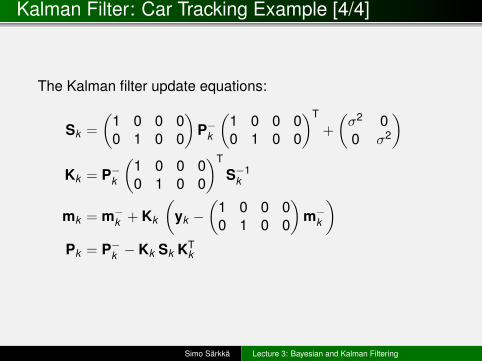
Kalman Filter: Car Tracking Example [4/4]
The Kalman filter update equations:
Sk =
(1 0 0 00 1 0 0
)P−k
(1 0 0 00 1 0 0
)T
+
(σ2 00 σ2
)Kk = P−k
(1 0 0 00 1 0 0
)T
S−1k
mk = m−k + Kk
(yk −
(1 0 0 00 1 0 0
)m−k
)Pk = P−k − Kk Sk KT
k
Simo Särkkä Lecture 3: Bayesian and Kalman Filtering
Summary
Probabilistic state space models consist of Markoviandynamic models and conditionally independentmeasurement models.Special cases are, for example, linear Gaussian modelsand non-linear and non-Gaussian models.Bayesian filtering equations form the formal solution togeneral Bayesian filtering problem.The Bayesian filtering equations consist of prediction andupdate steps.Kalman filter is the closed form filtering solution to linearGaussian models.
Simo Särkkä Lecture 3: Bayesian and Kalman Filtering
Matlab Demo: Kalman Filter Implementation
[Kalman filter for car tracking model]
Simo Särkkä Lecture 3: Bayesian and Kalman Filtering