Embed Size (px)
Citation preview

Lecture 3
HYPOTHESIS TESTS
Introduction
Recall that confidence intervals can be used to make inferencesabout the population mean µ:
Introduction
Recall that confidence intervals can be used to make inferencesabout the population mean µ:
A confidence interval is “better” than a point estimate on it’sown – we now have a range of values for µ;
Introduction
Recall that confidence intervals can be used to make inferencesabout the population mean µ:
A confidence interval is “better” than a point estimate on it’sown – we now have a range of values for µ;
If the confidence intervals for two (independent) samplesoverlap, then we can be ‘confident’ that there is no realdifference between the population means;
If a confidence interval for µ captures a ‘target value’, thenwe can be ’confident’ that the population mean might beequal to this value.
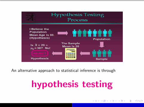
An alternative approach to statistical inference is through
hypothesis testing
Hypothesis tests
A hypothesis test is a rule for establishing whether or not a set ofdata is consistent with a hypothesis about a parameter of interest.
Hypothesis tests
A hypothesis test is a rule for establishing whether or not a set ofdata is consistent with a hypothesis about a parameter of interest.
We have two hypotheses:
Hypothesis tests
A hypothesis test is a rule for establishing whether or not a set ofdata is consistent with a hypothesis about a parameter of interest.
We have two hypotheses:
the null hypothesis (H0), and
Hypothesis tests
A hypothesis test is a rule for establishing whether or not a set ofdata is consistent with a hypothesis about a parameter of interest.
We have two hypotheses:
the null hypothesis (H0), and
the alternative hypothesis (H1)
Hypothesis tests
A hypothesis test is a rule for establishing whether or not a set ofdata is consistent with a hypothesis about a parameter of interest.
We have two hypotheses:
the null hypothesis (H0), and
the alternative hypothesis (H1)
and we want to see if the null hypothesis can be ”disproved” ornot.
If we can’t “disprove” the null hypothesis, then we go with itand the alternative is discarded.
Conversely, if we “disprove” the null hypothesis, we have analternative to go with!
An illustrative example
Suppose you are going on holiday to Kavos in March. Before youleave, a friend tells you that Kavos has an average of 10 hourssunshine a day during March.
On the first three days of your holiday there are 7, 8 and 9 hoursof sunshine respectively. You consider that this is evidence thatyour friend is wrong.
Thus, the null hypothesis would state that the average sunshinehours per day is 10 (as suggested by your friend):
H0 : µ = 10
An illustrative example
Your alternative hypothesis might state that the average sunshinehours per day is less than 10:
An illustrative example
Your alternative hypothesis might state that the average sunshinehours per day is less than 10:
H1 : µ < 10
An illustrative example
Your alternative hypothesis might state that the average sunshinehours per day is less than 10:
H1 : µ < 10
You might be tempted to go with the alternative hypothesis, sinceon your first three days you have observed less than 10 hours ofsunshine.
An illustrative example
Your alternative hypothesis might state that the average sunshinehours per day is less than 10:
H1 : µ < 10
You might be tempted to go with the alternative hypothesis, sinceon your first three days you have observed less than 10 hours ofsunshine.
However, this sample of three days could be a fluke result – youmight have chosen the most miserable period in March for yearsfor your holiday.Your test results are not conclusive; they only give you
evidence against a particular belief and we should be aware
of the weight of that evidence.
Other possible alternative hypotheses could have been:
H1 : µ > 10 or maybe
H1 : µ 6= 10

Decision time...
We need to go with either the null or the alternative, and we canuse statistics to help us decide!
Hypothesis tests can help us to choose between the null and thealternative.
Methodology for hypothesis testing
All hypothesis tests follow the same basic framework:
Methodology for hypothesis testing
All hypothesis tests follow the same basic framework:
1. State the null hypothesis
Methodology for hypothesis testing
All hypothesis tests follow the same basic framework:
1. State the null hypothesis
Say what your null hypothesis is! If you’re asked to test if thepopulation mean is equal to 10, for example, then you’d write
H0 : µ = 10.
Methodology for hypothesis testing
All hypothesis tests follow the same basic framework:
1. State the null hypothesis
Say what your null hypothesis is! If you’re asked to test if thepopulation mean is equal to 10, for example, then you’d write
H0 : µ = 10.
Or if you’re asked to find out if two population means are equal,you’d write
H0 : µ1 = µ2

2. State the alternative hypothesis
2. State the alternative hypothesis
This is what else could happen! For example, you could use
H1 : µ 6= 10;
2. State the alternative hypothesis
This is what else could happen! For example, you could use
H1 : µ 6= 10;
thus is known as a two–tailed or general alternative.
2. State the alternative hypothesis
This is what else could happen! For example, you could use
H1 : µ 6= 10;
thus is known as a two–tailed or general alternative.
Or if your sample suggests that the mean is considerably lower,you might use
H1 : µ < 10, or perhaps

2. State the alternative hypothesis
This is what else could happen! For example, you could use
H1 : µ 6= 10;
thus is known as a two–tailed or general alternative.
Or if your sample suggests that the mean is considerably lower,you might use
H1 : µ < 10, or perhaps
H1 : µ > 10
if you think it might be higher. These are known as one–tailedalternatives.

3. Calculate the test statistic
3. Calculate the test statistic
We use the data to calculate this. Often it has a common senseinterpretation (as we’ll see)!

4. Find the p–value
4. Find the p–value
This is the probability of observing the data if the null hypothesis
is true.
4. Find the p–value
This is the probability of observing the data if the null hypothesis
is true.
Equivalently, the p-value is the probability of observing somethingas extreme as the test statistic if the null hypothesis is true.
4. Find the p–value
This is the probability of observing the data if the null hypothesis
is true.
Equivalently, the p-value is the probability of observing somethingas extreme as the test statistic if the null hypothesis is true.Obviously, if this probability is small, then either we’ve observedsomething rare OR it looks like the null hypothesis is garbage!
You’ll see how to obtain this value shortly, and we’ll discuss whatwe mean by a “small” p–value.

5. Form a conclusion

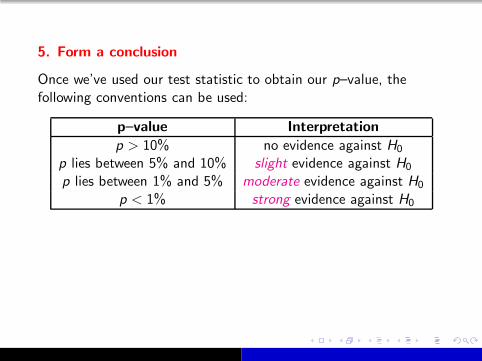
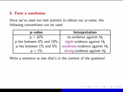
5. Form a conclusion
Once we’ve used our test statistic to obtain our p–value, thefollowing conventions can be used:
5. Form a conclusion
Once we’ve used our test statistic to obtain our p–value, thefollowing conventions can be used:
p–value Interpretation
p > 10% no evidence against H0
p lies between 5% and 10% slight evidence against H0
p lies between 1% and 5% moderate evidence against H0
p < 1% strong evidence against H0
Write a sentence or two that’s in the context of the question!
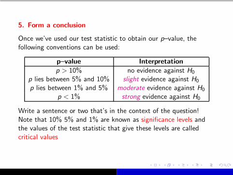
5. Form a conclusion
Once we’ve used our test statistic to obtain our p–value, thefollowing conventions can be used:
p–value Interpretation
p > 10% no evidence against H0
p lies between 5% and 10% slight evidence against H0
p lies between 1% and 5% moderate evidence against H0
p < 1% strong evidence against H0
Write a sentence or two that’s in the context of the question!Note that 10% 5% and 1% are known as significance levels andthe values of the test statistic that give these levels are calledcritical values
Testing one mean
From a single population we draw a single sample. We’d like touse the information in this sample to see how convincing aproposal for the population mean is.
Testing one mean
From a single population we draw a single sample. We’d like touse the information in this sample to see how convincing aproposal for the population mean is.
Just like in the construction of confidence intervals, there are twosituations which will determine the details of the test:
Testing one mean
From a single population we draw a single sample. We’d like touse the information in this sample to see how convincing aproposal for the population mean is.
Just like in the construction of confidence intervals, there are twosituations which will determine the details of the test:
The population variance (σ2) is known;
The population variance (σ2) is unknown.
Case 1: Known population variance σ2
If the population variance is known, we:
Case 1: Known population variance σ2
If the population variance is known, we:
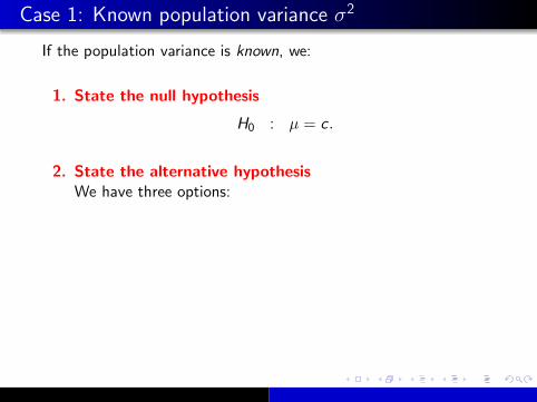
1. State the null hypothesis
H0 : µ = c .
Case 1: Known population variance σ2
If the population variance is known, we:
1. State the null hypothesis
H0 : µ = c .
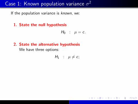
2. State the alternative hypothesis
We have three options:
Case 1: Known population variance σ2
If the population variance is known, we:
1. State the null hypothesis
H0 : µ = c .
2. State the alternative hypothesis
We have three options:
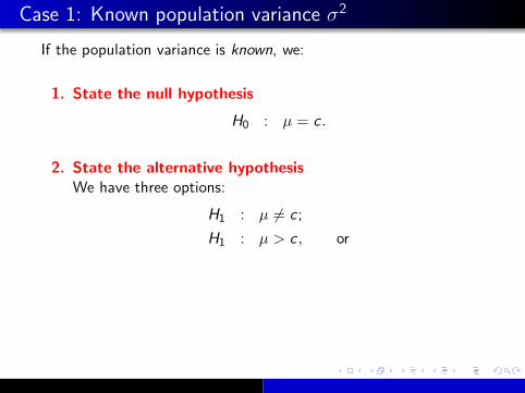
H1 : µ 6= c ;
Case 1: Known population variance σ2
If the population variance is known, we:
1. State the null hypothesis
H0 : µ = c .
2. State the alternative hypothesis
We have three options:
H1 : µ 6= c ;
H1 : µ > c , or

Case 1: Known population variance σ2
If the population variance is known, we:
1. State the null hypothesis
H0 : µ = c .
2. State the alternative hypothesis
We have three options:
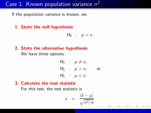
H1 : µ 6= c ;
H1 : µ > c , or
H1 : µ < c .
Case 1: Known population variance σ2
If the population variance is known, we:
1. State the null hypothesis
H0 : µ = c .
2. State the alternative hypothesis
We have three options:
H1 : µ 6= c ;
H1 : µ > c , or
H1 : µ < c .
3. Calculate the test statistic
For this test, the test statistic is
z =|x̄ − µ|√
σ2/n.

4. Find the p–value
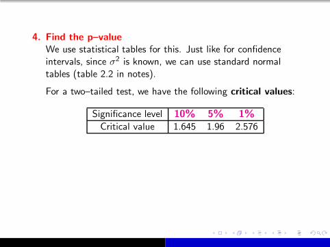
We use statistical tables for this. Just like for confidenceintervals, since σ2 is known, we can use standard normaltables (table 2.2 in notes).
4. Find the p–value
We use statistical tables for this. Just like for confidenceintervals, since σ2 is known, we can use standard normaltables (table 2.2 in notes).
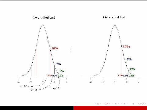
For a two–tailed test, we have the following critical values:
Significance level 10% 5% 1%
Critical value 1.645 1.96 2.576
4. Find the p–value
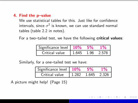
We use statistical tables for this. Just like for confidenceintervals, since σ2 is known, we can use standard normaltables (table 2.2 in notes).
For a two–tailed test, we have the following critical values:
Significance level 10% 5% 1%
Critical value 1.645 1.96 2.576
Similarly, for a one–tailed test we have:
Significance level 10% 5% 1%
Critical value 1.282 1.645 2.326
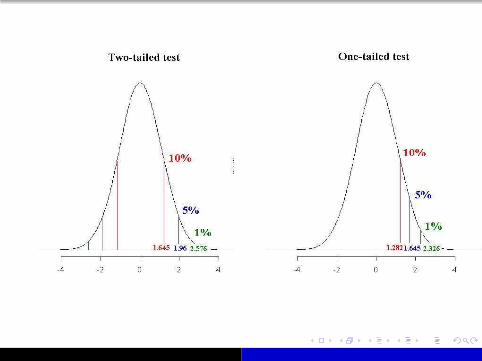
A picture might help! (Page 15)


5. Form a conclusion
Use table 2.1 in the notes to go with the null hypothesis orthe alternative hypothesis!
Don’t forget to write a sentence or two in the context of thequestion!
Example 2.4.1 (page 17)
A chain of shops believes that the average size of transactions is£130, and the variance is known to be £900.
The takings of one branch were analysed and it was found that themean transaction size was £123 over the 100 transactions in oneday. Based on this sample, test the null hypothesis that the truemean is equal to £130.
Since σ2 is known (we are given that σ2 = 900), we use theapproach just discussed.

Example 2.4.1 (page 17)
Steps 1 and 2 (hypotheses)Here, we state our null and alternative hypotheses. The nullhypothesis is given in the question – i.e.

Example 2.4.1 (page 17)
Steps 1 and 2 (hypotheses)Here, we state our null and alternative hypotheses. The nullhypothesis is given in the question – i.e.
H0 : µ = £130.
Example 2.4.1 (page 17)
Steps 1 and 2 (hypotheses)Here, we state our null and alternative hypotheses. The nullhypothesis is given in the question – i.e.
H0 : µ = £130.
We could test against a general (two–tailed) alternative, i.e.
H1 : µ 6= £130.

Example 2.4.1 (page 17)
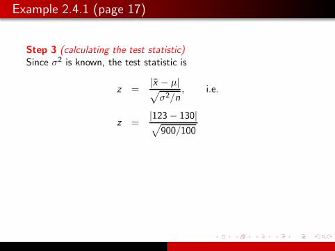
Step 3 (calculating the test statistic)Since σ2 is known, the test statistic is
Example 2.4.1 (page 17)
Step 3 (calculating the test statistic)Since σ2 is known, the test statistic is
z =|x̄ − µ|√
σ2/n, i.e.
Example 2.4.1 (page 17)
Step 3 (calculating the test statistic)Since σ2 is known, the test statistic is
z =|x̄ − µ|√
σ2/n, i.e.
z =|123 − 130|√
900/100

Example 2.4.1 (page 17)
Step 3 (calculating the test statistic)Since σ2 is known, the test statistic is
z =|x̄ − µ|√
σ2/n, i.e.
z =|123 − 130|√
900/100
=7√9
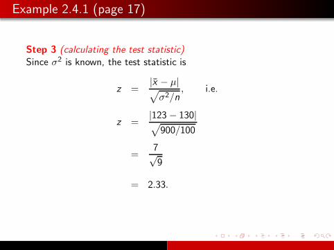
Example 2.4.1 (page 17)
Step 3 (calculating the test statistic)Since σ2 is known, the test statistic is
z =|x̄ − µ|√
σ2/n, i.e.
z =|123 − 130|√
900/100
=7√9
= 2.33.
Example 2.4.1 (page 17)
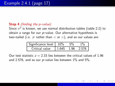
Step 4 (finding the p–value)Since σ2 is known, we use normal distribution tables (table 2.2) toobtain a range for our p–value. Our alternative hypothesis istwo–tailed (i.e. 6= rather than < or >), and so our values are:
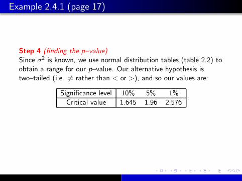
Example 2.4.1 (page 17)
Step 4 (finding the p–value)Since σ2 is known, we use normal distribution tables (table 2.2) toobtain a range for our p–value. Our alternative hypothesis istwo–tailed (i.e. 6= rather than < or >), and so our values are:
Significance level 10% 5% 1%
Critical value 1.645 1.96 2.576
Our test statistic z = 2.33 lies between the critical values of 1.96and 2.576, and so our p–value lies between 1% and 5%.
Example 2.4.1 (page 17)
Step 5 (conclusion)Using table 2.1 to interpret our p–value, we see that there ismoderate evidence against H0.
Thus, we should reject H0 in favour of the alternative hypothesisH1; it appears that the population mean transaction size is notequal to £130.
Example 2.4.1 (page 17)
Alternatively, suppose we suspect that the proposed value of £130is too high. We could have set up a one–tailed alternativehypothesis in step 2, i.e we could have tested
Example 2.4.1 (page 17)
Alternatively, suppose we suspect that the proposed value of £130is too high. We could have set up a one–tailed alternativehypothesis in step 2, i.e we could have tested
H0 : µ = £130 against
Example 2.4.1 (page 17)
Alternatively, suppose we suspect that the proposed value of £130is too high. We could have set up a one–tailed alternativehypothesis in step 2, i.e we could have tested
H0 : µ = £130 against
H1 : µ < £130.

Example 2.4.1 (page 17)
This is now a one–tailed test and the critical values from table 2.2are

Example 2.4.1 (page 17)
This is now a one–tailed test and the critical values from table 2.2are
Significance level 10% 5% 1%
Critical value 1.282 1.645 2.326

Example 2.4.1 (page 17)
This is now a one–tailed test and the critical values from table 2.2are
Significance level 10% 5% 1%
Critical value 1.282 1.645 2.326
The test statistic is (as before) 2.33, which now lies “to the right”of the last critical value in the table (2.326).

Example 2.4.1 (page 17)
This is now a one–tailed test and the critical values from table 2.2are
Significance level 10% 5% 1%
Critical value 1.282 1.645 2.326
The test statistic is (as before) 2.33, which now lies “to the right”of the last critical value in the table (2.326).
Thus, our p–value is now smaller than 1%, and so, using table 2.1,we see that in this more specific test there is strong evidenceagainst H0.

Example 2.4.1 (page 17)
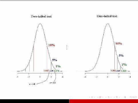
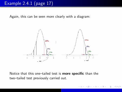
Again, this can be seen more clearly with a diagram:
Example 2.4.1 (page 17)
Again, this can be seen more clearly with a diagram:
Notice that this one–tailed test is more specific than thetwo–tailed test previously carried out.

Example 2.4.1 (page 17)
Again, this can be seen more clearly with a diagram:
Notice that this one–tailed test is more specific than thetwo–tailed test previously carried out.
Unknown population variance σ2
If the population variance is unknown, things are more awkward!Steps 1 and 2 are the same, i.e.
Unknown population variance σ2
If the population variance is unknown, things are more awkward!Steps 1 and 2 are the same, i.e.
1. State the null hypothesis
Unknown population variance σ2
If the population variance is unknown, things are more awkward!Steps 1 and 2 are the same, i.e.
1. State the null hypothesis
2. State the alternative hypothesis

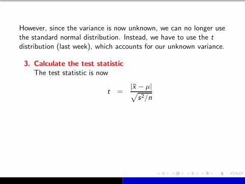
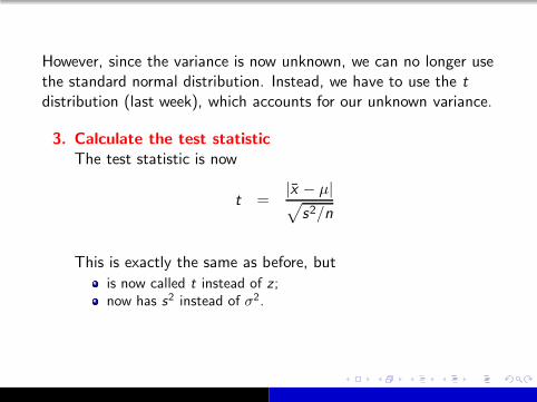
However, since the variance is now unknown, we can no longer usethe standard normal distribution. Instead, we have to use the tdistribution (last week), which accounts for our unknown variance.
However, since the variance is now unknown, we can no longer usethe standard normal distribution. Instead, we have to use the tdistribution (last week), which accounts for our unknown variance.
3. Calculate the test statistic
The test statistic is now
t =|x̄ − µ|√
s2/n
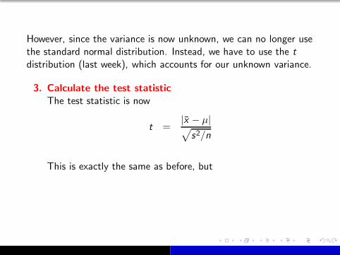
However, since the variance is now unknown, we can no longer usethe standard normal distribution. Instead, we have to use the tdistribution (last week), which accounts for our unknown variance.
3. Calculate the test statistic
The test statistic is now
t =|x̄ − µ|√
s2/n
This is exactly the same as before, but
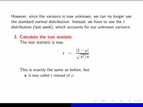
is now called t instead of z ;
However, since the variance is now unknown, we can no longer usethe standard normal distribution. Instead, we have to use the tdistribution (last week), which accounts for our unknown variance.
3. Calculate the test statistic
The test statistic is now
t =|x̄ − µ|√
s2/n
This is exactly the same as before, but
is now called t instead of z ;now has s2 instead of σ2.

4. Find the p–value
This is the same as when we calculated confidence intervalsfor the “unknown variance” situation: we need to uset–tables, with degrees of freedom ν = n − 1.
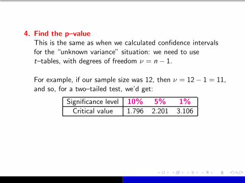
4. Find the p–value
This is the same as when we calculated confidence intervalsfor the “unknown variance” situation: we need to uset–tables, with degrees of freedom ν = n − 1.
For example, if our sample size was 12, then ν = 12− 1 = 11,and so, for a two–tailed test, we’d get:
Significance level 10% 5% 1%
Critical value 1.796 2.201 3.106
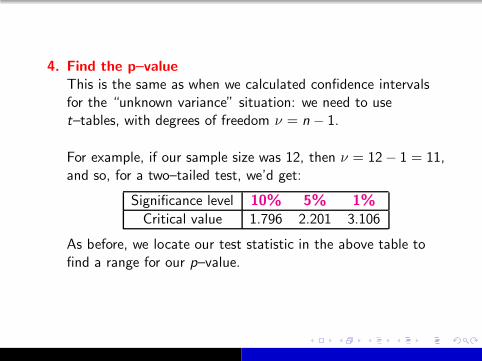
As before, we locate our test statistic in the above table tofind a range for our p–value.

5. Form a conclusion
Exactly the same as before – use table 2.1 to help you!

Example 2.4.2 (page 19)
The batteries for a fire alarm system are required to last for 20000hours before they need replacing.
16 batteries were tested; they were found to have an average life of19500 hours and a standard deviation of 1200 hours.
Perform a hypothesis test to see if the batteries do, on average,last for 20000 hours.
Example 2.4.2 (page 19)
Steps 1 and 2 (hypotheses)Using a one–tailed test, our null and alternative hypotheses are:
Example 2.4.2 (page 19)
Steps 1 and 2 (hypotheses)Using a one–tailed test, our null and alternative hypotheses are:
H0 : µ = 20000 versus
Example 2.4.2 (page 19)
Steps 1 and 2 (hypotheses)Using a one–tailed test, our null and alternative hypotheses are:
H0 : µ = 20000 versus
H1 : µ < 20000.
Example 2.4.2 (page 19)
Step 3 (calculating the test statistic)The population variance σ2 is now unknown – the question doesnot say
Example 2.4.2 (page 19)
Step 3 (calculating the test statistic)The population variance σ2 is now unknown – the question doesnot say
“the population variance is . . . ”
Example 2.4.2 (page 19)
Step 3 (calculating the test statistic)The population variance σ2 is now unknown – the question doesnot say
“the population variance is . . . ”
“the population standard deviation is . . . ”
Example 2.4.2 (page 19)
Step 3 (calculating the test statistic)The population variance σ2 is now unknown – the question doesnot say
“the population variance is . . . ”
“the population standard deviation is . . . ”
“σ = . . .”
Example 2.4.2 (page 19)
Step 3 (calculating the test statistic)The population variance σ2 is now unknown – the question doesnot say
“the population variance is . . . ”
“the population standard deviation is . . . ”
“σ = . . .”
the process variance is . . . ”
Example 2.4.2 (page 19)
Step 3 (calculating the test statistic)The population variance σ2 is now unknown – the question doesnot say
“the population variance is . . . ”
“the population standard deviation is . . . ”
“σ = . . .”
the process variance is . . . ”
However, the sample standard deviation is given, based on asample of size 16, and so we can use the t distribution.

Example 2.4.2 (page 19)
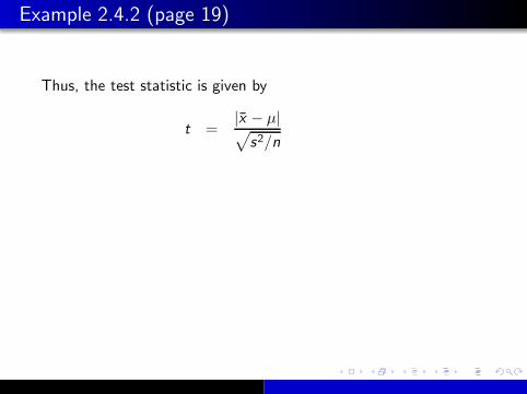
Thus, the test statistic is given by
Example 2.4.2 (page 19)
Thus, the test statistic is given by
t =|x̄ − µ|√
s2/n
Example 2.4.2 (page 19)
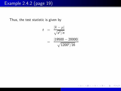
Thus, the test statistic is given by
t =|x̄ − µ|√
s2/n
=|19500 − 20000|√
12002/16
Example 2.4.2 (page 19)
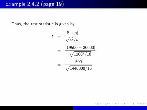
Thus, the test statistic is given by
t =|x̄ − µ|√
s2/n
=|19500 − 20000|√
12002/16
=500
√
1440000/16
Example 2.4.2 (page 19)
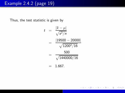
Thus, the test statistic is given by
t =|x̄ − µ|√
s2/n
=|19500 − 20000|√
12002/16
=500
√
1440000/16
= 1.667.

Example 2.4.2 (page 19)
Step 4 (finding the p–value)Since σ2 is unknown, we use t–distribution tables (table 2.3) toobtain a range for our p–value.

Example 2.4.2 (page 19)
Step 4 (finding the p–value)Since σ2 is unknown, we use t–distribution tables (table 2.3) toobtain a range for our p–value.
The degrees of freedom, ν = n − 1 = 16− 1 = 15, and under aone–tailed test this gives the following critical values:

Example 2.4.2 (page 19)
Step 4 (finding the p–value)Since σ2 is unknown, we use t–distribution tables (table 2.3) toobtain a range for our p–value.
The degrees of freedom, ν = n − 1 = 16− 1 = 15, and under aone–tailed test this gives the following critical values:
Significance level 10% 5% 1%
Critical value 1.341 1.753 2.602
Our test statistic of t = 1.667 lies between the critical values of1.341 and 1.753, and so the corresponding p–value lies between5% and 10%.
Example 2.4.2 (page 19)
Step 5 (conclusion)Using table 2.1 to interpret our p–value, we see that there is onlyslight evidence against the null hypothesis and certainly notenough grounds to reject it, so we retain H0.
It is plausible that, on average, the batteries do last for 20000hours.