Lecture 3 Laplace transform Ing. Jaroslav Jíra, CSc. Physics for informatics

Lecture 3Laplace transform

Ing. Jaroslav Jíra, CSc.

Physics for informatics

What is it good for?

The Laplace transform

• Solving of differential equations

• System modeling

• System response analysis

• Process control application

Solving of differential equations procedure


1. Finding differential equations describing the system

2. Obtaining the Laplace transform of these equations

3. Performing simple algebra to solve for output or variable of interest

4. Applying inverse transform to find solution

A system analysis can be done by several simple steps

The definition


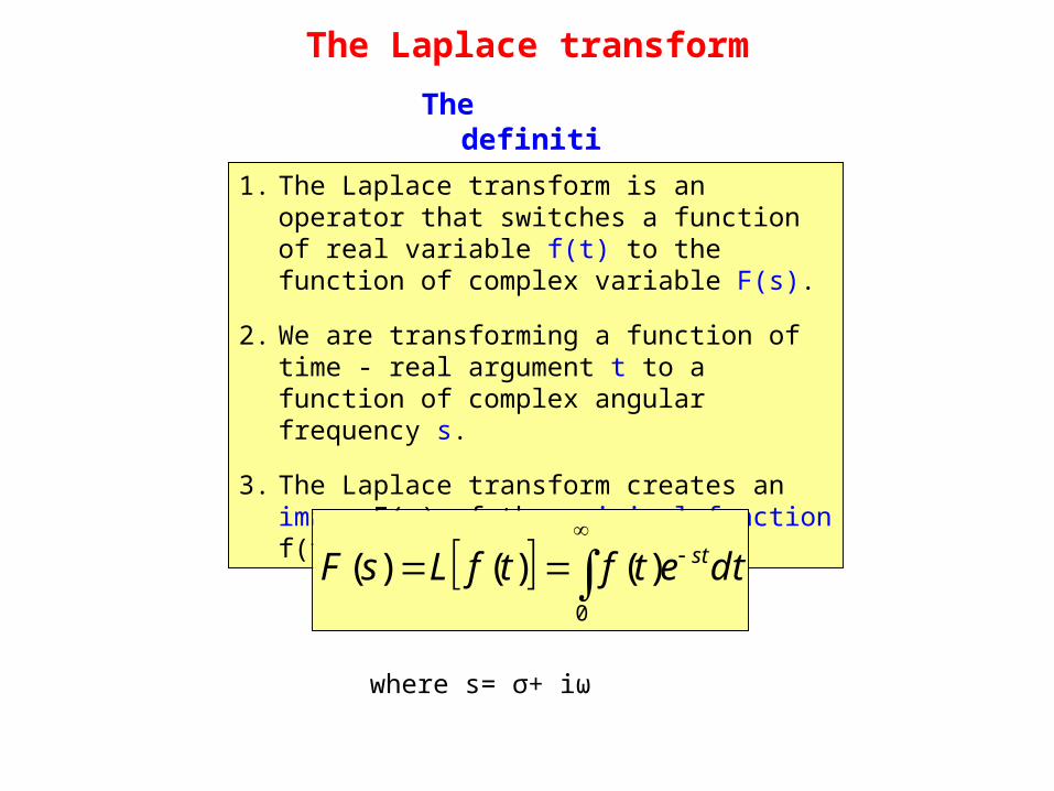
1. The Laplace transform is an operator that switches a function of real variable f(t) to the function of complex variable F(s).

2. We are transforming a function of time - real argument t to a function of complex angular frequency s.

3. The Laplace transform creates an image F(s) of the original function f(t)

0

)()()( dtetftfLsF st

where s= σ+ iω

Restrictions


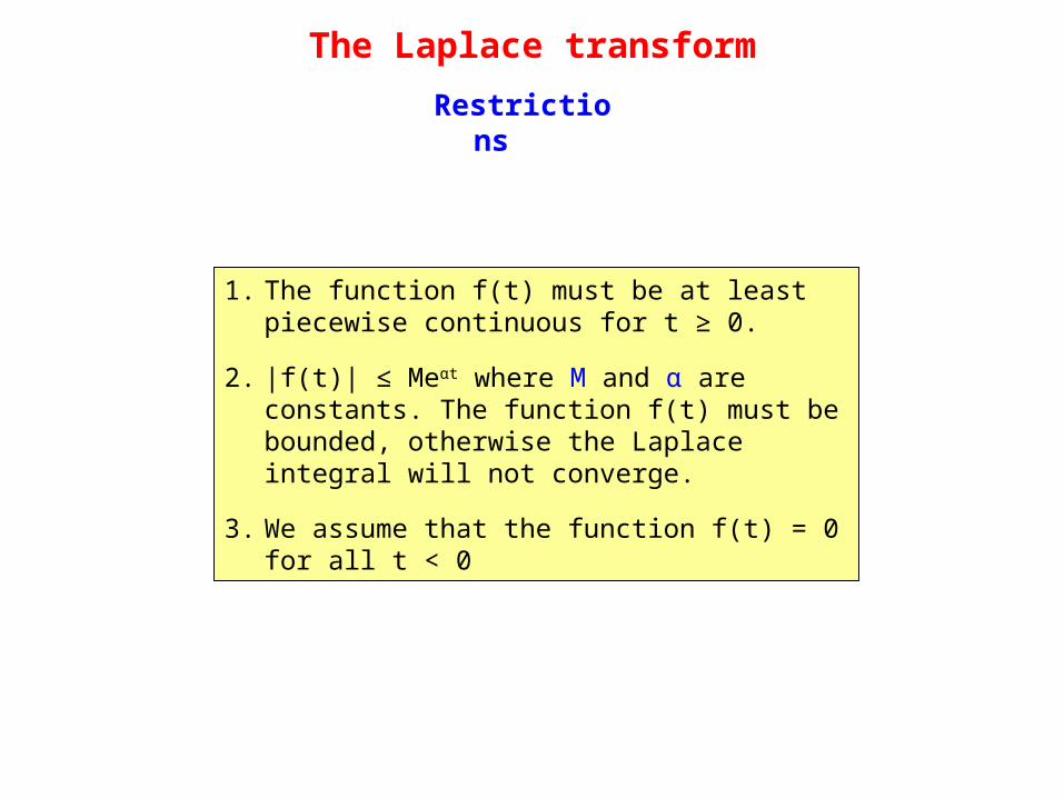
1. The function f(t) must be at least piecewise continuous for t ≥ 0.

2. |f(t)| ≤ Meαt where M and α are constants. The function f(t) must be bounded, otherwise the Laplace integral will not converge.

3. We assume that the function f(t) = 0 for all t < 0

Inverse Laplace transform


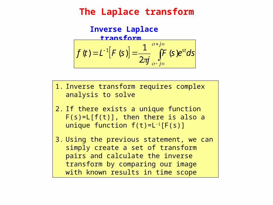
1. Inverse transform requires complex analysis to solve

2. If there exists a unique function F(s)=L[f(t)], then there is also a unique function f(t)=L-1[F(s)]

3. Using the previous statement, we can simply create a set of transform pairs and calculate the inverse transform by comparing our image with known results in time scope

j

j

stdsesFj

sFLtf

)(

2

1)()( 1

Basic properties


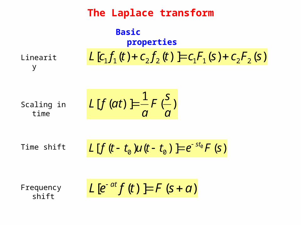
Linearity )()()]()([ 22112211 sFcsFctfctfcL

)(1

)]([a

sFa

atfL Scaling in time

Time shift

Frequency shift

)()]()([ 000 sFettuttfL st

)()]([ asFtfeL at

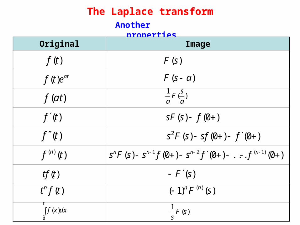
Another properties


Original Image

)(tf

t

dxxf0

)(

)(tf

)(atf

atetf )(

)(tf

)()( tf n

)(ttf

)(tft n

)0()0()(2 fsfsFs

)0(...)0()0()( )1(21 nnnn ffsfssFs

)(sF

)()1( )( sF nn

)(1

sFs

)0()( fssF

)(1

a

sFa

)( asF

)(sF

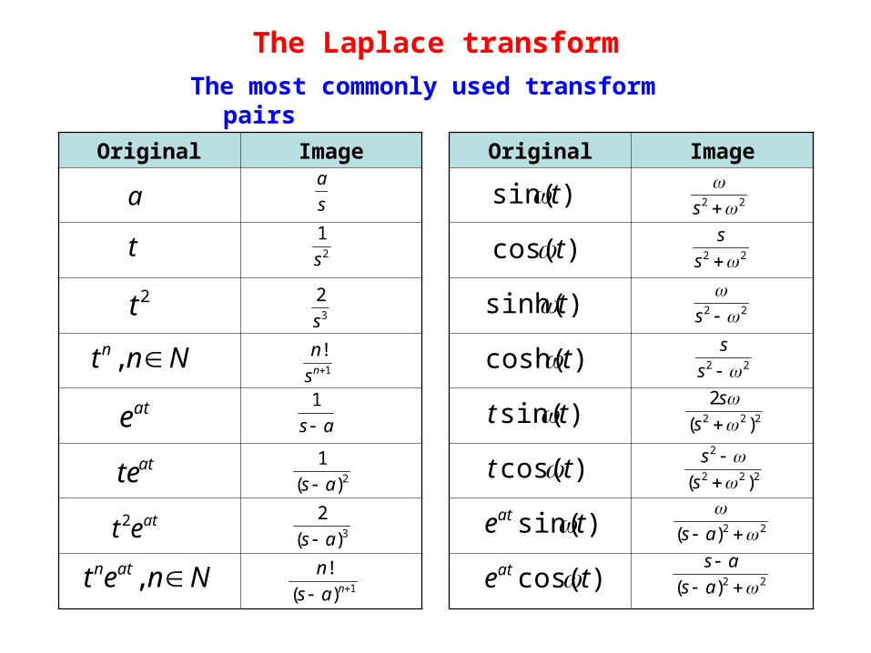
The most commonly used transform pairs


Original Image

t

ate

atte

atet 2

Nnt n ,

2t

Nnet atn ,

a

Original Image

)sinh( t

)cosh( t

)sin( tt

)cos( tt

)sin( teat

)cos( teat

)sin( t

)cos( t

s

a

2

1

s

3

2

s

1

!ns

n

as 1

2)(

1

as

3)(

2

as

1)(

! nas

n

22 s

22 ss

22 s

22 ss

222 )(

2

ss

222

2

)(

s

s

22)( as

22)( as

as

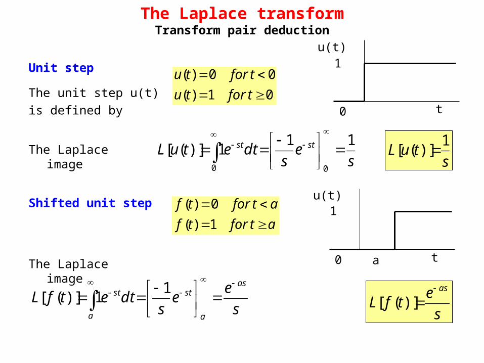
Unit step

The Laplace transformTransform pair deduction

01)(

00)(

tfortu

tfortu

se

sdtetuL stst 11

1)]([00

The unit step u(t)

is defined by

The Laplace image s

tuL1

)]([

Shifted unit step

t

1

0

u(t)

atfortf

atfortf

1)(

0)(

t

1

0

u(t)

aThe Laplace image

s

ee

sdtetfL

as

aa

stst

1

1)]([s

etfL

as

)]([

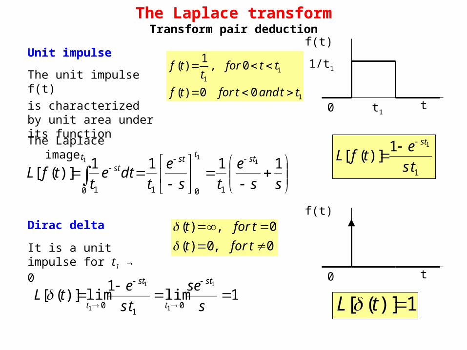
Unit impulse


1

11

00)(

0,1

)(

ttandtfortf

ttfort

tf

ss

e

ts

e

tdte

ttfL

sttt stst 1111

)]([1

11

100 11

The unit impulse f(t)

is characterized by unit area under its function

The Laplace image

t

1/t1

0

f(t)

It is a unit impulse for t1 → 0

1lim1

lim)]([1

1

1

1 01

0

s

se

ts

etL

st

t

st

t 1)]([ tL

t1

1

11)]([

ts

etfL

st

Dirac delta

0,0)(

0,)(

tfort

tfort

t0

f(t)

Exponential function


atetf )(

2

0

20 00

10

)(1)]()([

ss

edt

s

e

s

etdttetutfL

stststst

Linear function

asas

tasedtedteetutfL tasstat

1

)(

)()]()([

00

)(

0

aseat

1

ˆ

ttf )(

vuuvvu

0

)]()([ dttetutfL st

Per partes integration

s

evev

utust

st

;'

1';

2

1ˆs

t


200 00

22 122

02

)]()([ss

dttes

dts

te

s

etdtettutfL st

ststst

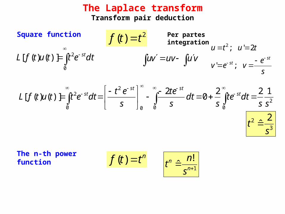
Square function 2)( ttf

vuuvvu

0

2)]()([ dtettutfL st


s

evev

tutust

st

;'

2';2

32 2ˆs

t

The n-th power function nttf )(1

!ˆ

nn

s

nt


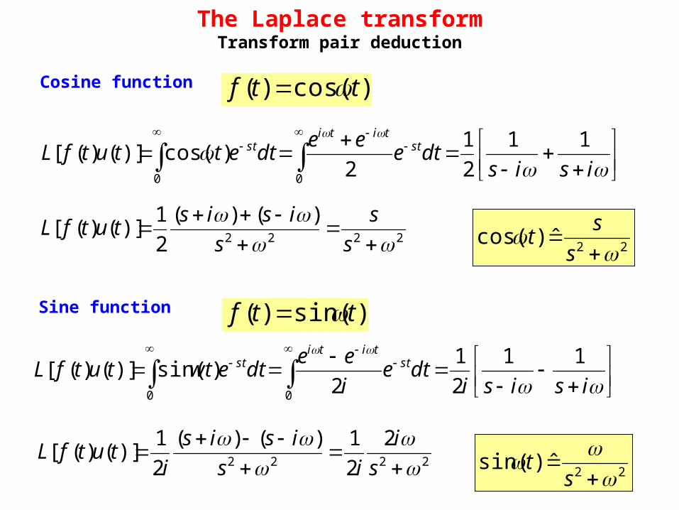
Cosine function )cos()( ttf

isisdte

eedtettutfL st

titist 11

2

1

2)cos()]()([

0 0

22ˆ)cos(

s

st2222

)()(

2

1)]()([

s

s

s

isistutfL

Sine function )sin()( ttf

isisidte

i

eedtewttutfL st

titist 11

2

1

2)sin()]()([

0 0

22ˆ)sin(

s

t2222

2

2

1)()(

2

1)]()([

s

i

is

isis

itutfL


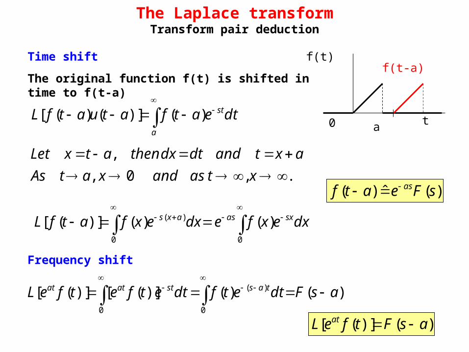
Time shift

a

stdteatfatuatfL )()]()([

)(ˆ)( sFeatf as

t0

f(t)

a

The original function f(t) is shifted in time to f(t-a)f(t-a)

.,0,

,

xtasandxatAs

axtanddtdxthenatxLet

0 0

)( )()()]([ dxexfedxexfatfL sxasaxs

Frequency shift

0

)(

0

)()()]([)]([ asFdtetfdtetfetfeL tasstatat

)()]([ asFtfeL at

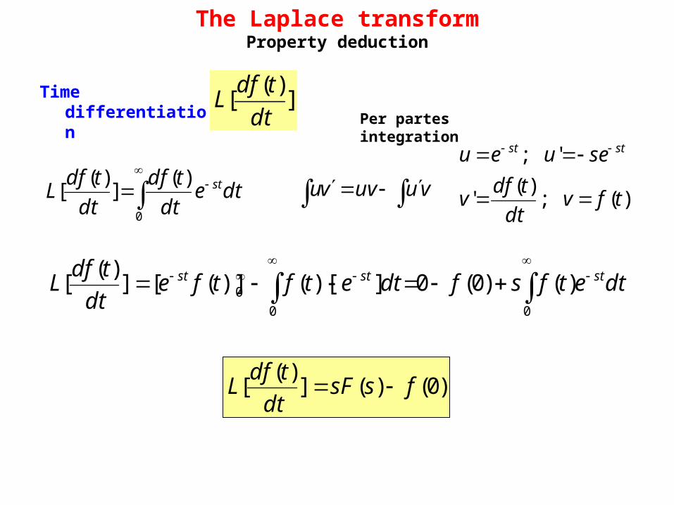
The Laplace transformProperty deduction

00

0 )()0(0])[()]([])(

[ dtetfsfdtetftfedt

tdfL ststst

Time differentiation ])(

[dt

tdfL

vuuvvu

0

)(])(

[ dtedt

tdf

dt

tdfL st


)(;)(

'

';

tfvdt

tdfv

seueu stst

)0()(])(

[ fssFdt

tdfL

The Laplace transformProperty deduction

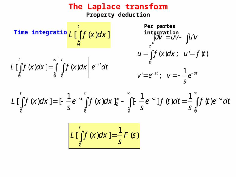
00

0

00

)(1

)(]1

[])(1

[])([ dtetfs

dttfes

dxxfes

dxxfL ststt

stt

Time integration ])([0t

dxxfL vuuvvu

0 00

)(])([ dtedxxfdxxfL sttt


stst

t

es

vev

tfudxxfu

1

;'

)(';)(0

)(1

])([0

sFs

dxxfLt

The algorithm of inverse Laplace transform


Since the F(s) is mostly fractional function, then the most important step is to perform partial fraction decomposition of it.

Depending on roots in denominator, we are looking for the following functions, where A and B are real numbers:

for a single real root s= a

for a double real root s= a

for a triple real root s= a

for a pair of pure imaginary roots s= ± iω

for a pair of complex conjugated roots s= a ± iω

as

A

as

B

as

A

2)(

as

C

as

B

as

A

23 )()(

22

s

BAs

22)( as

BAs

Two distinct real roots

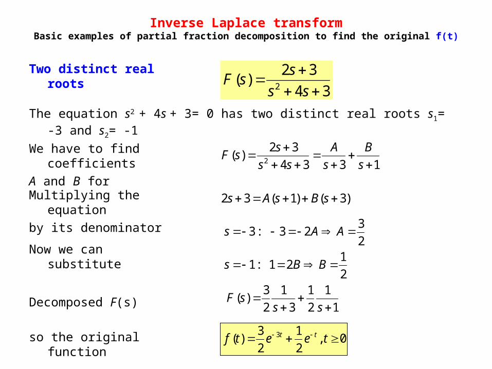
Inverse Laplace transformBasic examples of partial fraction decomposition to find the original f(t)

34

32)(

2

ss

ssF

1334

32)(

2

s

B

s

A

ss

ssF

)3()1(32 sBsAs

2

121:1

2

323:3

BBs

AAs

1

1

2

1

3

1

2

3)(

sssF

0,2

1

2

3)( 3 teetf tt

The equation s2 + 4s + 3= 0 has two distinct real roots s1= -3 and s2= -1

We have to find coefficients

A and B for

Multiplying the equation

by its denominator

Now we can substitute

Decomposed F(s)

so the original function

One real root

and one real double root


2

2

)3)(1(

53)(

ss

ssF

3)3(1)3)(1(

53)(

22

2

s

C

s

B

s

A

ss

ssF

)3)(1()1()3(53 22 ssCsBsAs

133:

16232:3

248:1

2

ACCAs

BBs

AAs

3

1

)3(

16

1

2)(

2

ssssF

0,162)( 33 teetetf ttt

The denominator has a single root s1= -1 and a double root s23= -3

We are looking for coefficients

A, B and C


by its denominator

Now we can substitute to get A,B;

the C coefficient can be obtained

by comparison of s2 factors

Decomposed F(s)


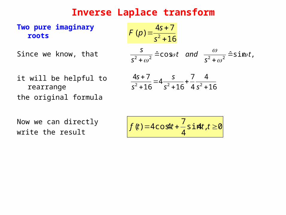
Two pure imaginary roots


16

74)(

2

s

spF

16

4

4

7

164

16

74222

ss

s

s

s

0,4sin4

74cos4)( ttttf

,sinˆcosˆ 2222t

sandt

s

s

Since we know, that

it will be helpful to rearrange

the original formula

Now we can directly

write the result

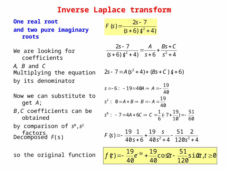
One real root

and two pure imaginary roots


)4)(6(

72)(

2

ss

ssF

46)4)(6(

7222

s

CBs

s

A

ss

s

)6)(()4(72 2 sCBssAs

60

51)

10

197(

6

1647:

40

190:

40

194019:6

0

2

CCAs

ABBAs

AAs

4

2

120

51

440

19

6

1

40

19)(

22

ss

s

ssF

0,2sin120

512cos

40

19

40

19)( 6 tttetf t

We are looking for coefficients

A, B and C


by its denominator

Now we can substitute to get A;

B,C coefficients can be obtained

by comparison of s0,s2 factors

Decomposed F(s)


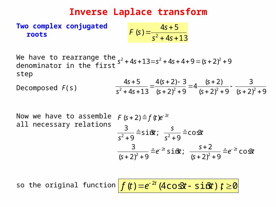
Two complex conjugated roots


134

54)(

2

ss

ssF

9)2(944134 222 sssss

9)2(

3

9)2(

)2(4

9)2(

3)2(4

134

542222

ss

s

s

s

ss

s

tes

ste

s

ts

st

s

etfsF

tt

t

3cosˆ9)2(

2;3sinˆ

9)2(

3

3cosˆ9

;3sinˆ9

3

)(ˆ)2(

22

22

22

2

0),3sin3cos4()( 2 tttetf t

We have to rearrange the denominator in the first step

Decomposed F(s)

Now we have to assemble all necessary relations


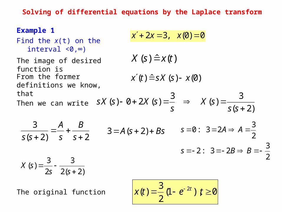
Example 1

Find the x(t) on the interval <0,∞)

Solving of differential equations by the Laplace transform

0)0(,32 xxx

)(ˆ)( txsX

)0()(ˆ)( xsXstx

)2(

3)(

3)(20)(

sssX

ssXsXs

0),1(2

3)( 2 tetx t

The image of desired function is

From the former definitions we know, that

Then we can write

2)2(

3

s

B

s

A

ssBssA )2(3

2

323:2

2

323:0

BBs

AAs

)2(2

3

2

3)(

sssX

The original function

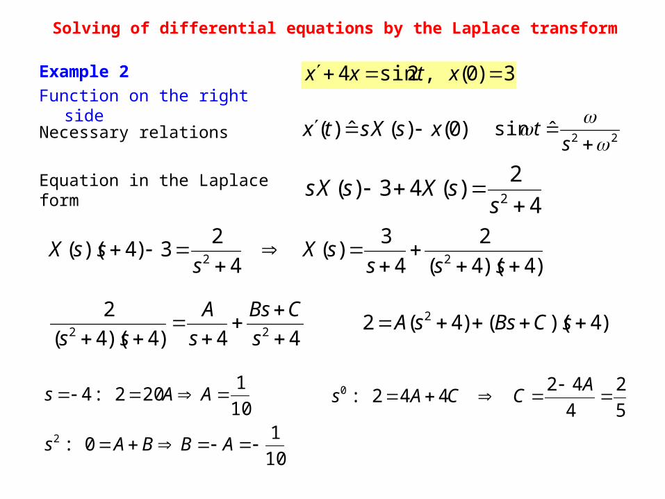
Example 2

Function on the right side


3)0(,2sin4 xtxx

22ˆsin

s

t)0()(ˆ)( xsXstx

4

2)(43)(

2 s

sXsXs

Necessary relations

Equation in the Laplace form

44)4)(4(

222

s

CBs

s

A

ss)4)(()4(2 2 sCBssA

10

10:

10

1202:4

2

ABBAs

AAs5

2

4

42442:0

ACCAs

)4)(4(

2

4

3)(

4

23)4)((

22

ssssX

sssX

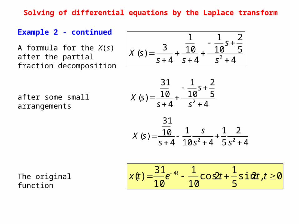
Example 2 - continued


452

101

4101

4

3)(

2

s

s

sssX

0,2sin5

12cos

10

1

10

31)( 4 tttetx t

A formula for the X(s) after the partial fraction decomposition

after some small arrangements


452

101

41031

)(2

s

s

ssX

4

2

5

1

410

1

41031

)(22

ss

s

ssX

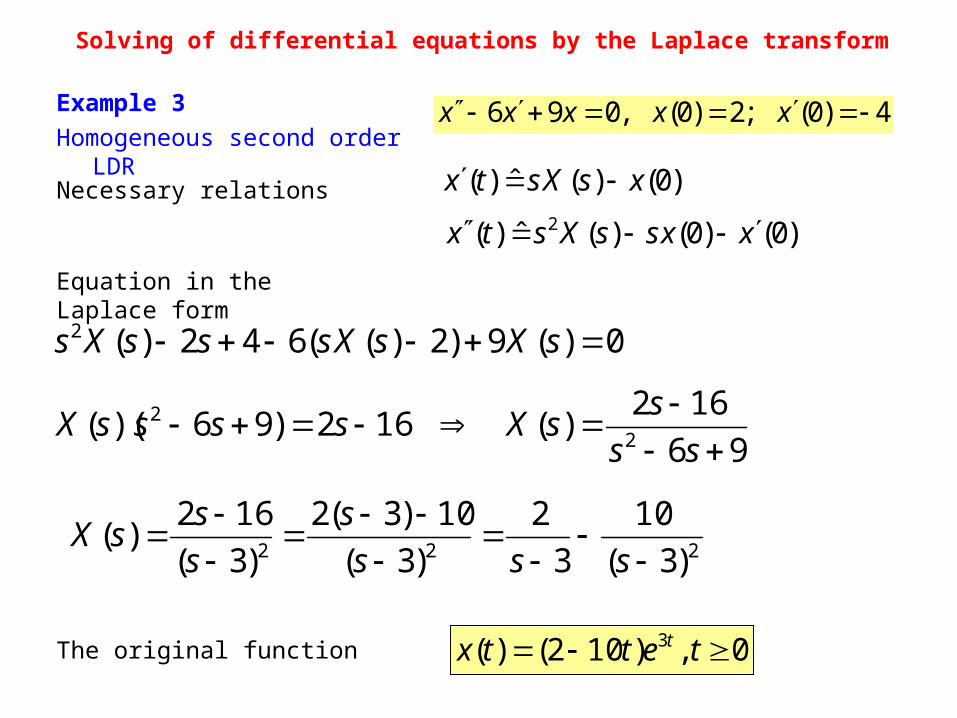
Example 3

Homogeneous second order LDR


4)0(;2)0(,096 xxxxx

0)(9)2)((642)(2 sXsXsssXs

)0()(ˆ)( xsXstx

0,)102()( 3 tettx t



Necessary relations

)0()0()(ˆ)( 2 xxssXstx

96

162)(162)96)((

22

ss

ssXssssX

222 )3(

10

3

2

)3(

10)3(2

)3(

162)(

sss

s

s

ssX

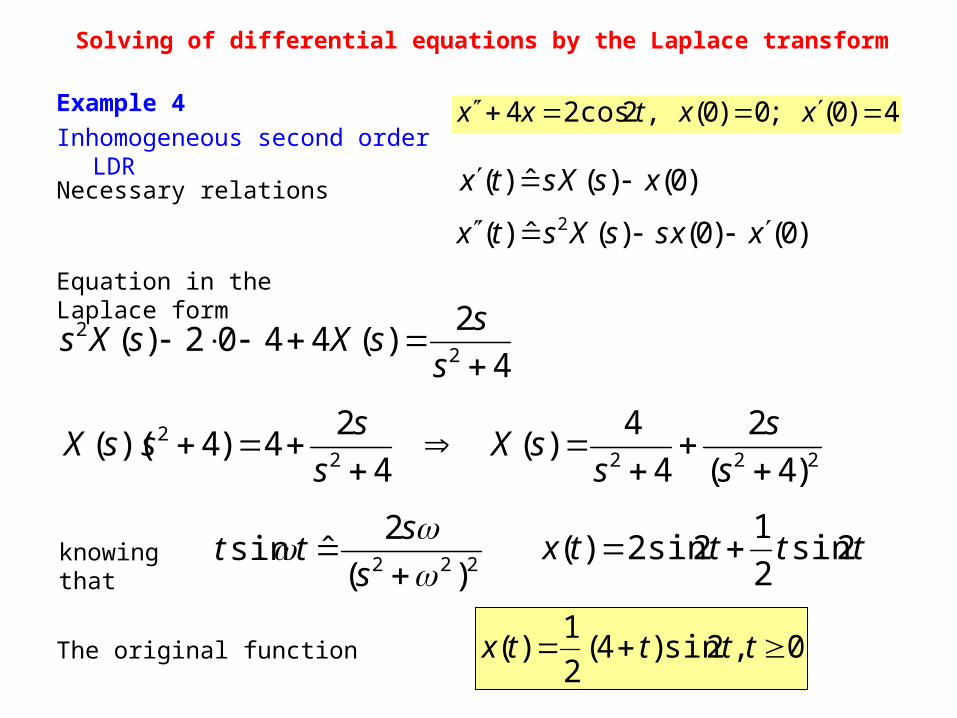
Example 4

Inhomogeneous second order LDR


4)0(;0)0(,2cos24 xxtxx

4

2)(4402)(

22

s

ssXsXs

)0()(ˆ)( xsXstx

0,2sin)4(2

1)( ttttx



Necessary relations

)0()0()(ˆ)( 2 xxssXstx

22222

)4(

2

4

4)(

4

24)4)((

s

s

ssX

s

sssX

ttttx 2sin2

12sin2)(

222 )(

2ˆsin

s

sttknowing that

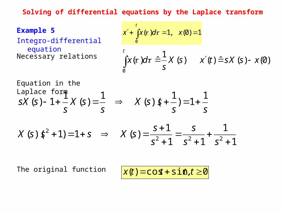
Example 5

Integro-differential equation


1)0(,1)(0

xdxxt

ssssX

ssX

sssX

11)

1)((

1)(

11)(

)0()(ˆ)( xsXstx

0,sincos)( ttttx



Necessary relations );(1ˆ)(

0

sXs

dxt

1

1

11

1)(1)1)((

2222

ss

s

s

ssXsssX

Documents

Lecture 3 Laplace transform Ing. Jaroslav Jíra, CSc. Physics for informatics