Lecture 3

Nonparametric density estimation and classification

Density estimation

Histogram

The box kernel -- Parzen window

K-nearest neighbor

Density estimation

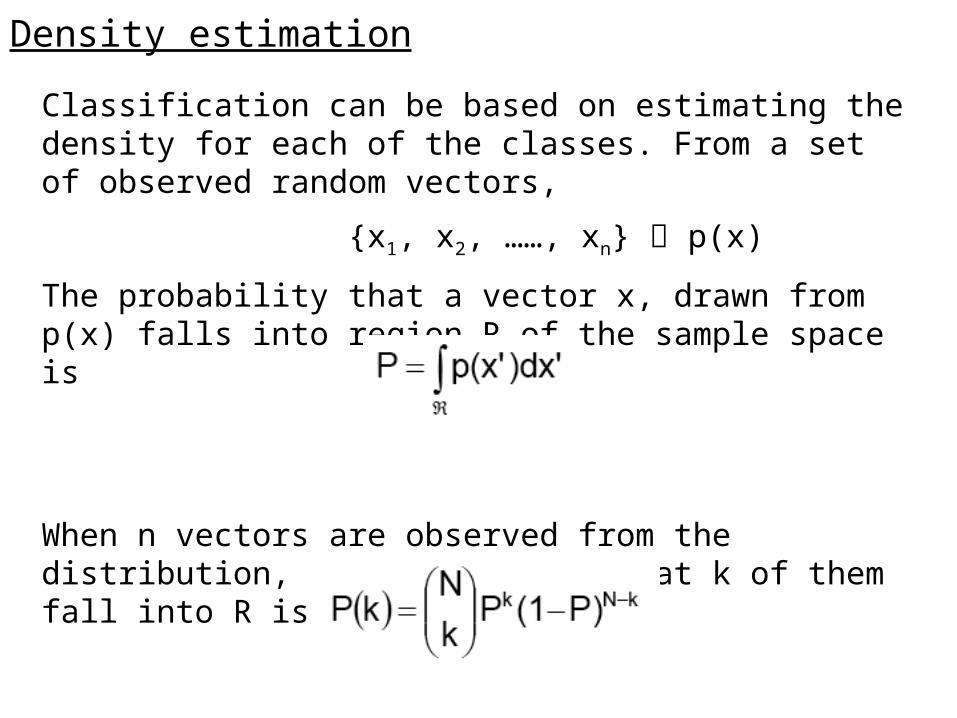
Classification can be based on estimating the density for each of the classes. From a set of observed random vectors,

{x1, x2, ……, xn} p(x)

The probability that a vector x, drawn from p(x) falls into region R of the sample space is

When n vectors are observed from the distribution, the probability that k of them fall into R is

Density estimation

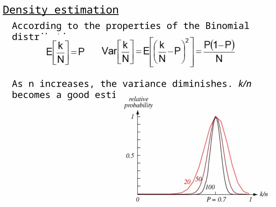
According to the properties of the Binomial distribution,

As n increases, the variance diminishes. k/n becomes a good estimator of P.

Density estimation

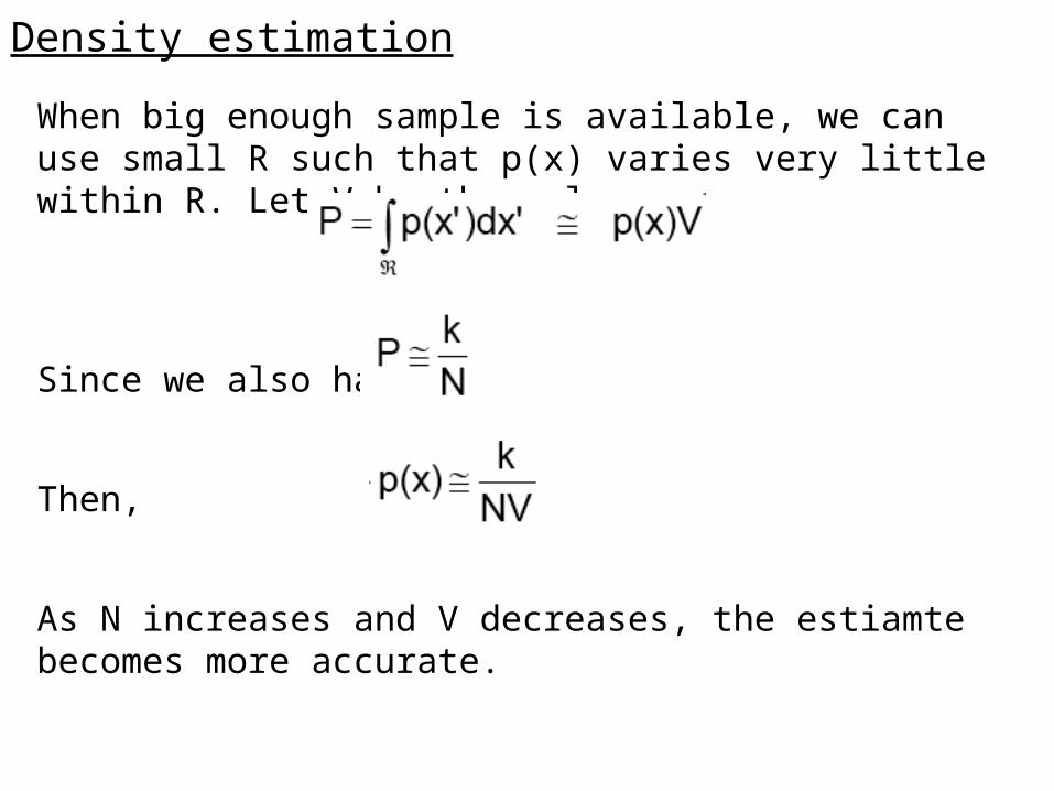
When big enough sample is available, we can use small R such that p(x) varies very little within R. Let V be the volume.

Since we also have

Then,

As N increases and V decreases, the estiamte becomes more accurate.

Density estimation

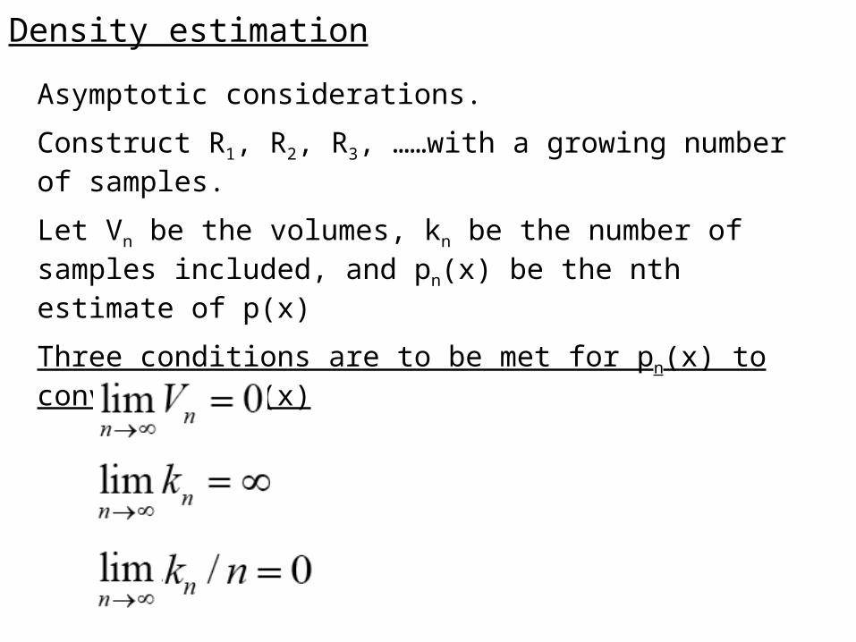
Asymptotic considerations.

Construct R1, R2, R3, ……with a growing number of samples.

Let Vn be the volumes, kn be the number of samples included, and pn(x) be the nth estimate of p(x)

Three conditions are to be met for pn(x) to converge to p(x)

Density estimation

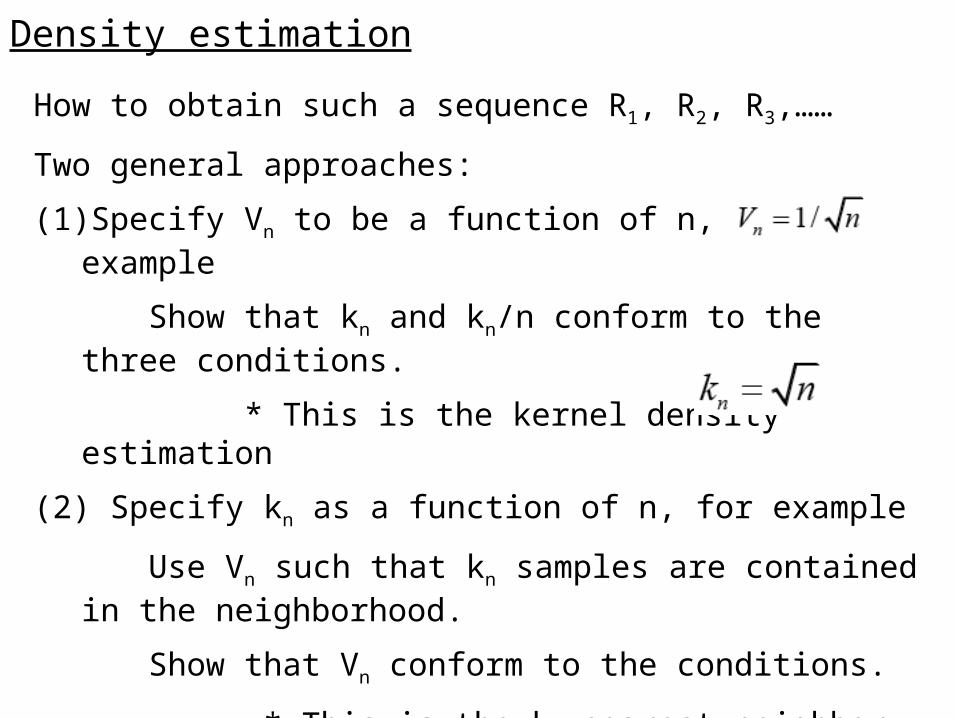
How to obtain such a sequence R1, R2, R3,……

Two general approaches:

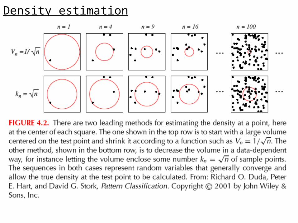
(1) Specify Vn to be a function of n, for example

Show that kn and kn/n conform to the three conditions.

* This is the kernel density estimation

(2) Specify kn as a function of n, for example

Use Vn such that kn samples are contained in the neighborhood.

Show that Vn conform to the conditions.

* This is the kn nearest neighbor method.

Density estimation

Histogram

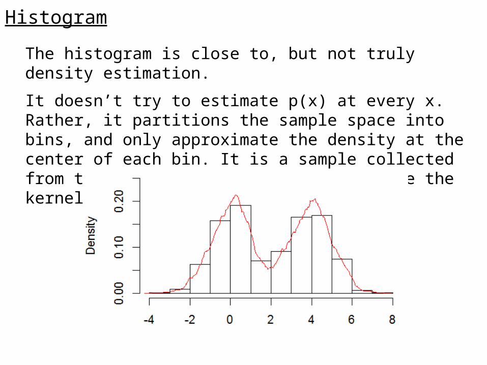
The histogram is close to, but not truly density estimation.

It doesn’t try to estimate p(x) at every x. Rather, it partitions the sample space into bins, and only approximate the density at the center of each bin. It is a sample collected from the kernel density estimation where the kernel is a box.

Histogram

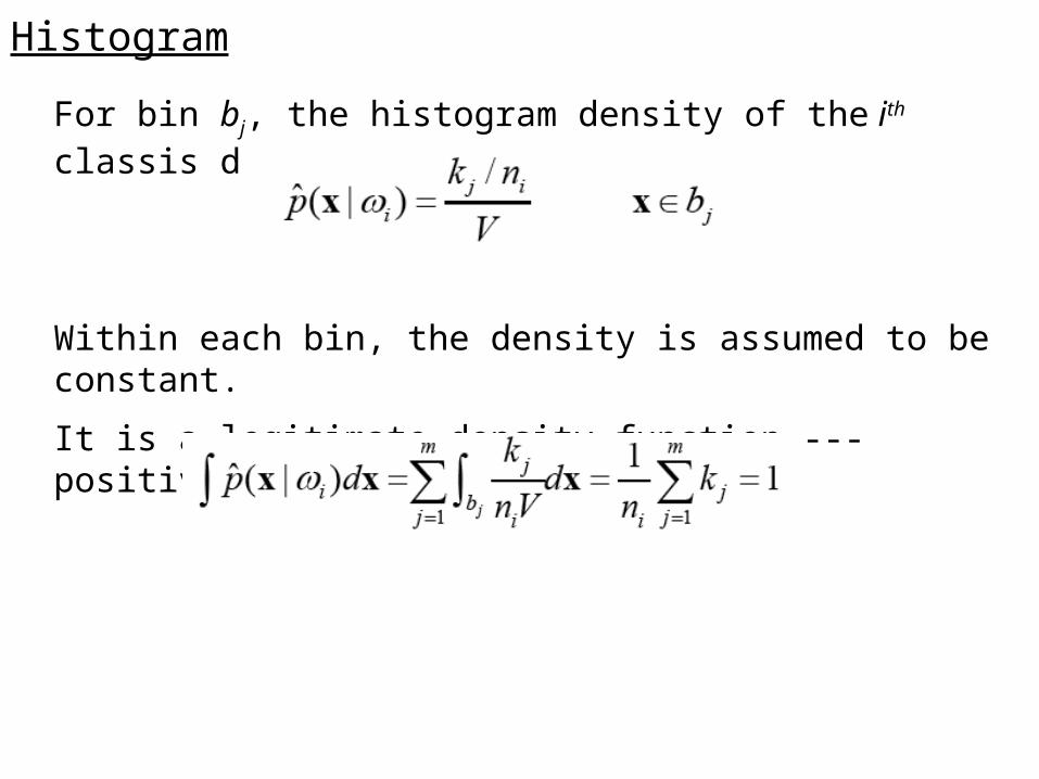
For bin bj, the histogram density of the ith classis defined as

Within each bin, the density is assumed to be constant.

It is a legitimate density function --- positive and integrate to one.

Histogram

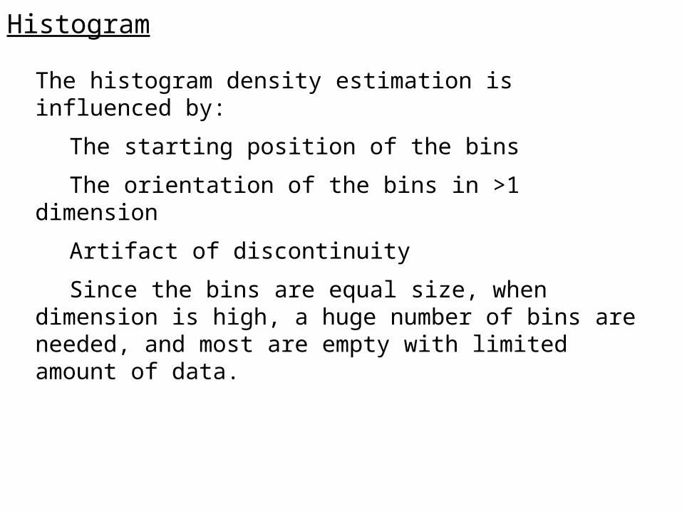
The histogram density estimation is influenced by:

The starting position of the bins

The orientation of the bins in >1 dimension

Artifact of discontinuity

Since the bins are equal size, when dimension is high, a huge number of bins are needed, and most are empty with limited amount of data.

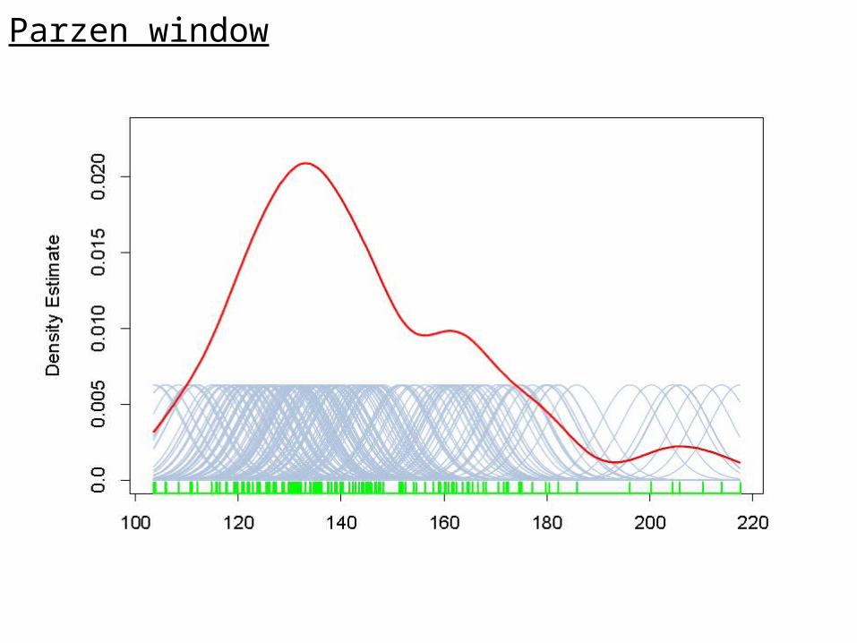
Parzen window

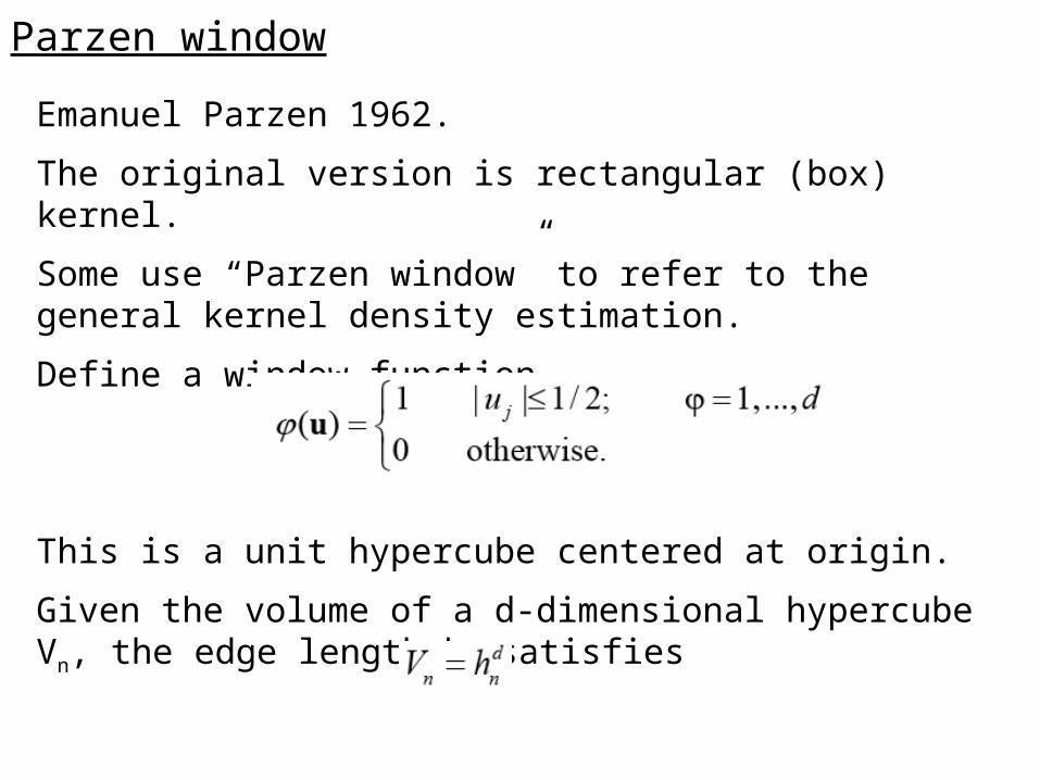
Emanuel Parzen 1962.

The original version is rectangular (box) kernel.

Some use “Parzen window” to refer to the general kernel density estimation.

Define a window function

This is a unit hypercube centered at origin.

Given the volume of a d-dimensional hypercube Vn, the edge length hn satisfies

Parzen window

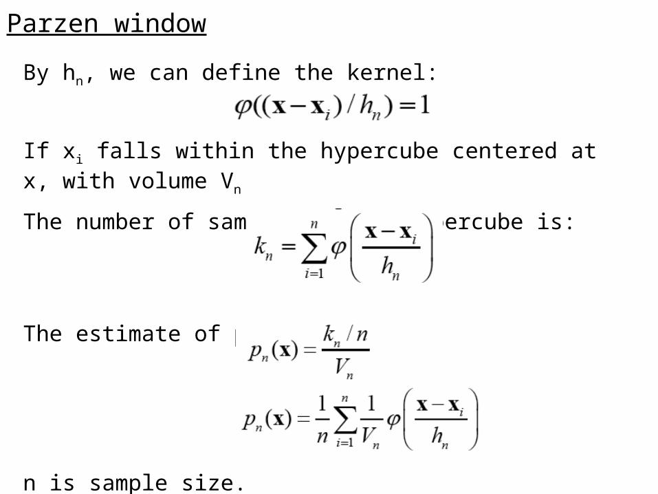
By hn, we can define the kernel:

If xi falls within the hypercube centered at x, with volume Vn

The number of samples in the hypercube is:

The estimate of p(x) is

n is sample size.

Parzen window

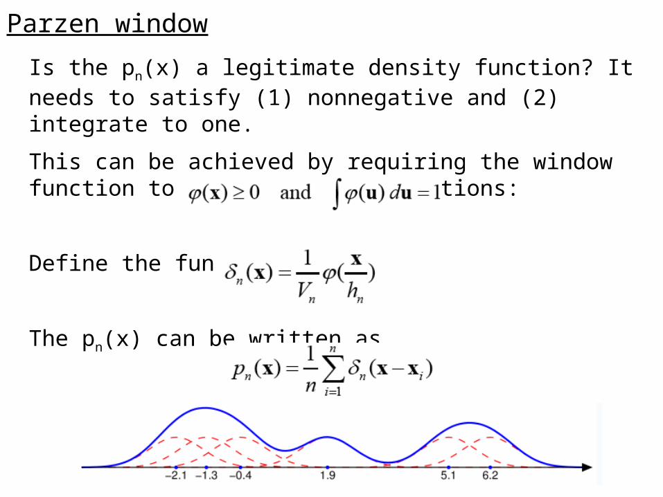
Is the pn(x) a legitimate density function? It needs to satisfy (1) nonnegative and (2) integrate to one.

This can be achieved by requiring the window function to satisfy these conditions:

Define the function

The pn(x) can be written as

Parzen window

Parzen window

n (x x i)dx 1

Vn

x x i

hn

dx (u)du 1

pn (x) 1

n n (x x i)

i

dx 1

nn (x x i)dx

i

1

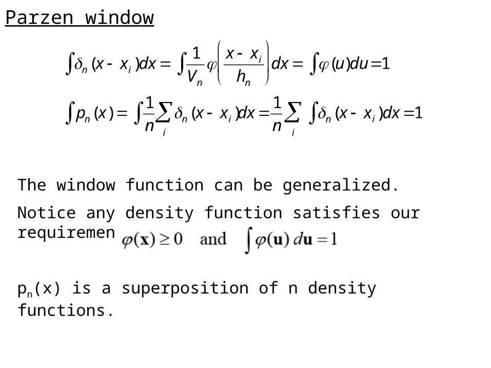
The window function can be generalized.

Notice any density function satisfies our requirement:

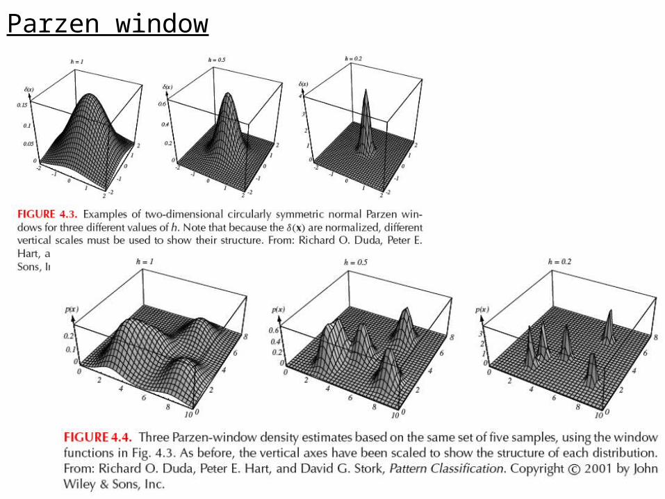
pn(x) is a superposition of n density functions.

Parzen window

Parzen window

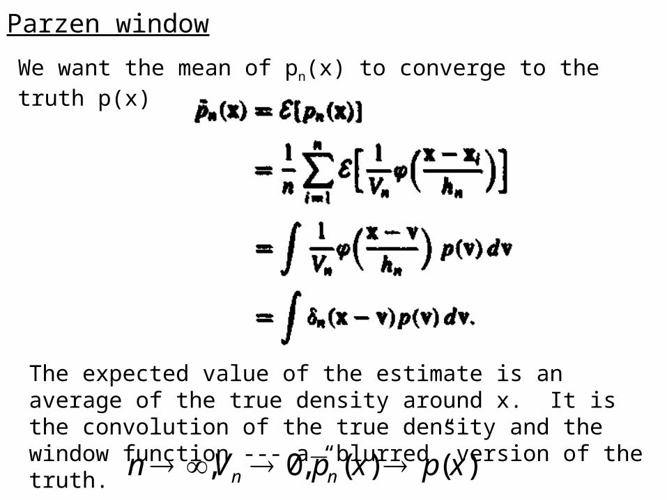
We want the mean of pn(x) to converge to the truth p(x)

The expected value of the estimate is an average of the true density around x. It is the convolution of the true density and the window function --- a “blurred” version of the truth.

When

n ,Vn 0, p n (x) p(x)

Parzen window

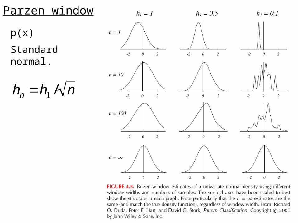
hn h1 / n

p(x)

Standard normal.

Parzen window

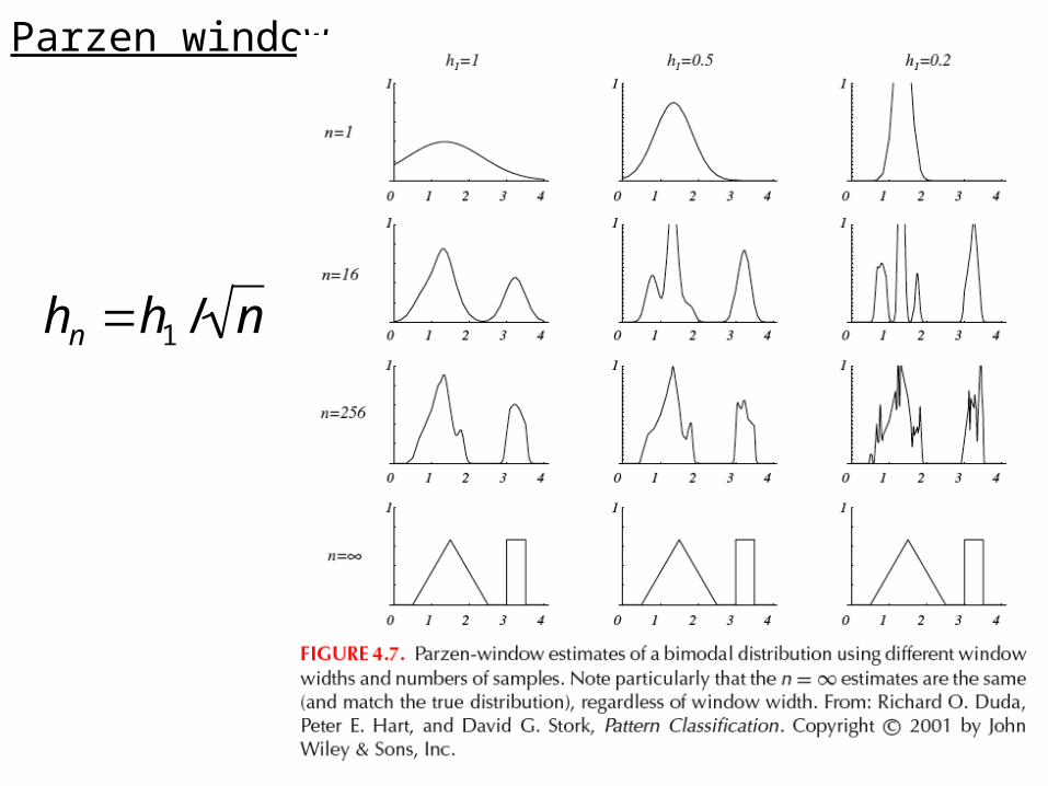
hn h1 / n

Parzen window

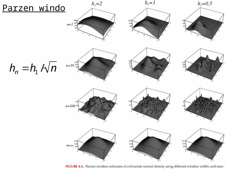
hn h1 / n

Parzen window classification

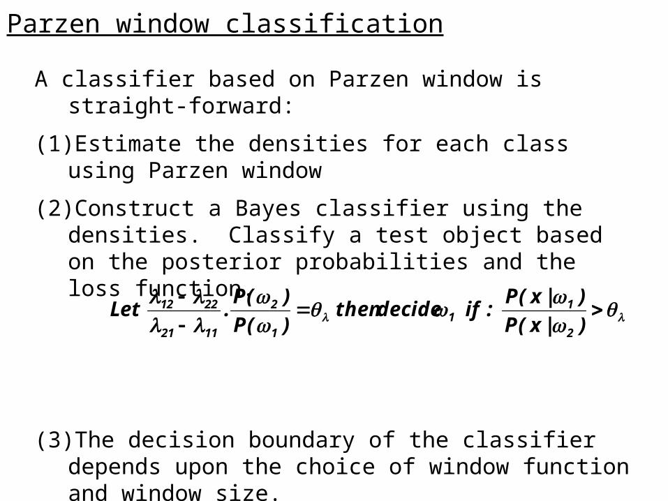
A classifier based on Parzen window is straight-forward:

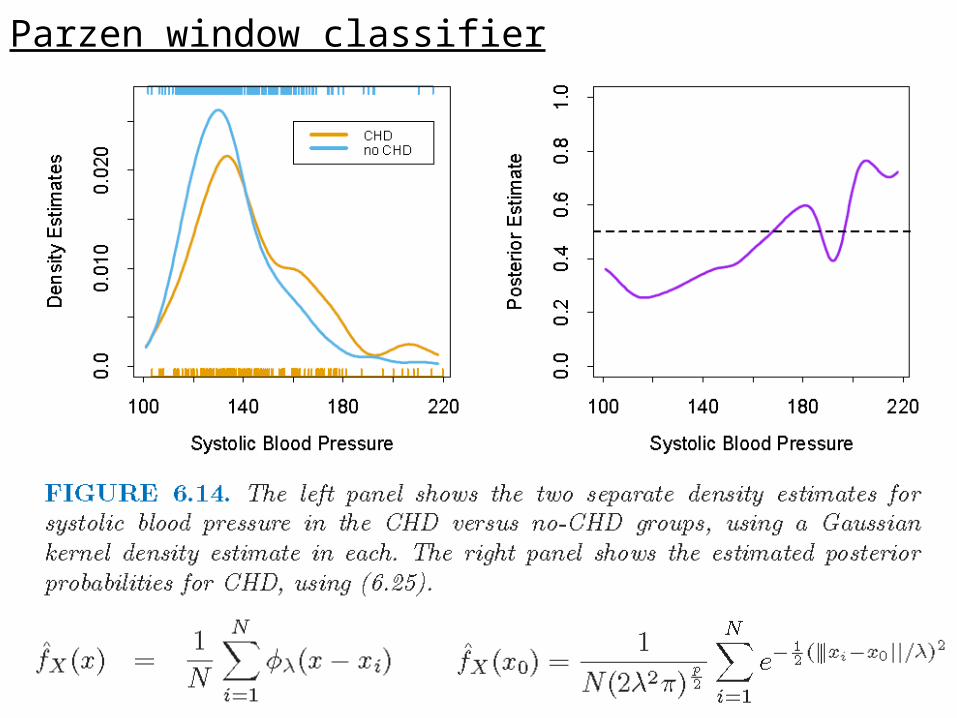
(1) Estimate the densities for each class using Parzen window

(2) Construct a Bayes classifier using the densities. Classify a test object based on the posterior probabilities and the loss function.

(3) The decision boundary of the classifier depends upon the choice of window function and window size.

)|x(P

)|x(P :if decide then

)(P

)(P. Let

2

11

1

2

1121

2212

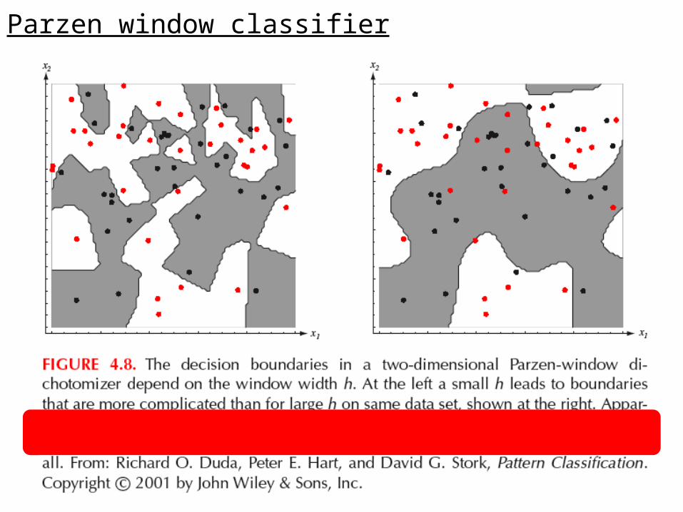
Parzen window classifier

Parzen window classifier

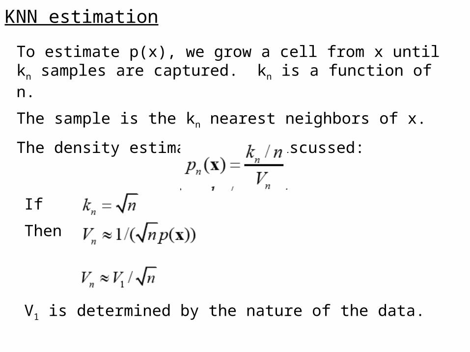
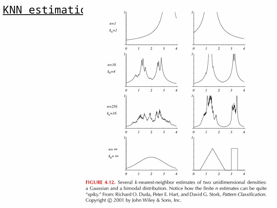
KNN estimation

To estimate p(x), we grow a cell from x until kn samples are captured. kn is a function of n.

The sample is the kn nearest neighbors of x.

The density estimate is as discussed:

If

Then

V1 is determined by the nature of the data.

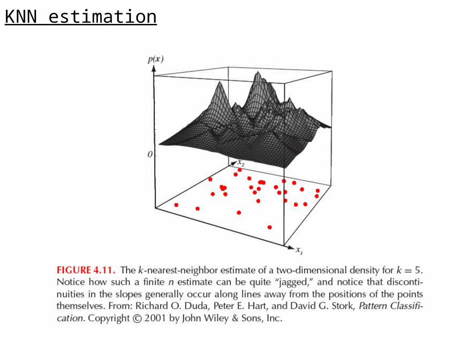
KNN estimation

KNN estimation

KNN classifier

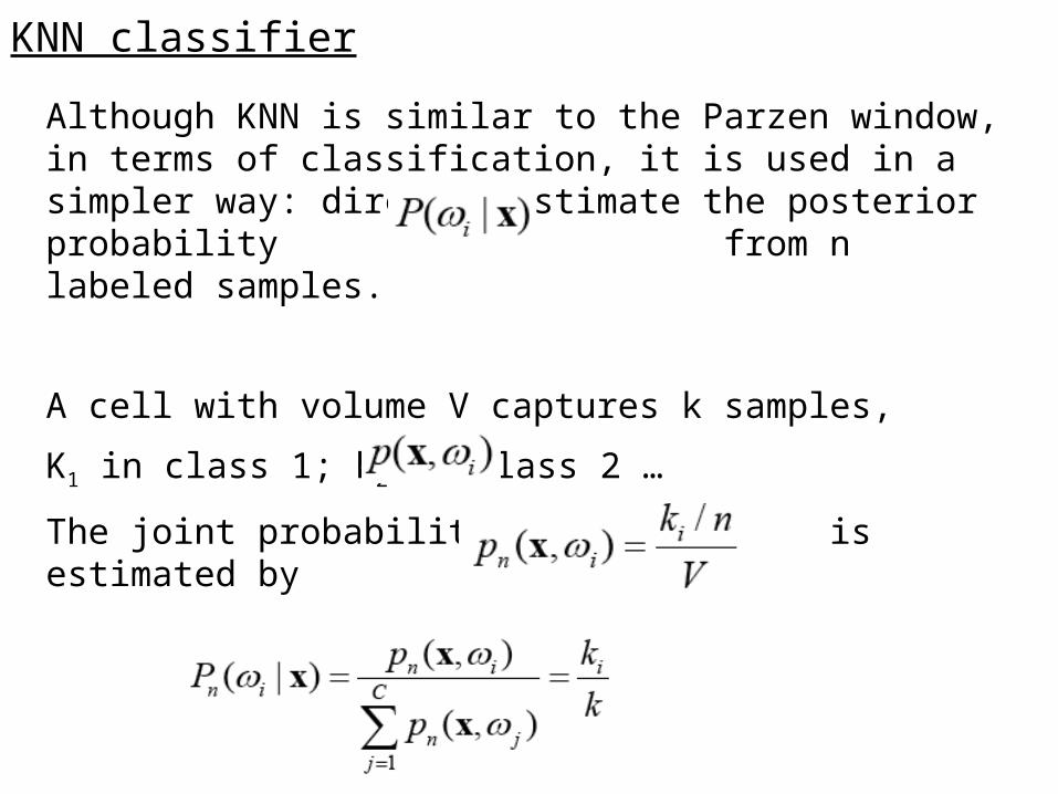
Although KNN is similar to the Parzen window, in terms of classification, it is used in a simpler way: directly estimate the posterior probability from n labeled samples.

A cell with volume V captures k samples,

K1 in class 1; k2 in class 2 …

The joint probability is estimated by

Then,

KNN classifier

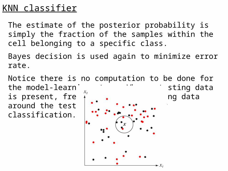
The estimate of the posterior probability is simply the fraction of the samples within the cell belonging to a specific class.

Bayes decision is used again to minimize error rate.

Notice there is no computation to be done for the model-learning step. When a testing data is present, frequencies from training data around the testing data is used for classification.

KNN classifier

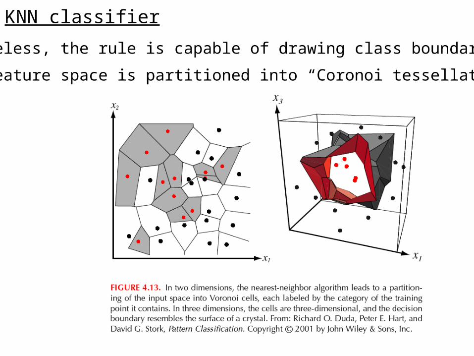
Nontheless, the rule is capable of drawing class boundaries.

The feature space is partitioned into “Coronoi tessellation”

KNN error

KNN doesn’t reach Bayes error rate. Here’s why:

The true posterior probabilities are known.

The Bayes decision rule will choose class 1. But will KNN always do that? No. KNN is influenced by sampling variations. It chooses class 1 with probability:

The larger the k, the smaller the error.

KNN error

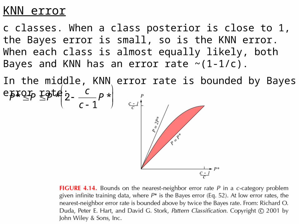
c classes. When a class posterior is close to 1, the Bayes error is small, so is the KNN error. When each class is almost equally likely, both Bayes and KNN has an error rate ~(1-1/c).

In the middle, KNN error rate is bounded by Bayes error rate:

P* P P * 2 c

c 1P *