148

Lecture 32. TORSION EXAMPLES HAVING MORE THANONE DEGREE OF FREEDOM

Torsional Vibration ExamplesWe worked through a one-degree-of-freedom, torsional-

vibration example in section 5.4, starting with the model offigure 5.10. Figure 5.35 illustrates a two-degree-of-freedomextension to this example. The upper disk has mass m1 , radiusR1 , and is connected to “ground” by a circular shaft of radius

length L1 , and shear modulus G1 . The lower disk has massm2, radius R2 , and is connected to disk 1 by a circular shaft ofradius , length L2 , and shear modulus G2 . The rotationangles and define the orientations of the two disks. Theshafts have zero elastic deflections and moments when theseangles are zero.

Figure 5.40 (a) Two-disk, torsionalvibration example, (b) coordinatesand free-body diagram for

149

(5.144)

(5.145)

As with the example of figure 5.10, twisting the upper diskthrough the angle will develop the reaction moment,

acting on top of the upper disk. The negative sign in thisequation implies that the moment is acting in a directionopposite to a positive rotation direction. The reactionmoment acting on the bottom of disk 1 and the top of disk 2 isproportional to the difference between the rotation angles and . Assuming that is greater than , the reactionmoment acting on disk 1 from the lower shaft is

The positive sign for the moment implies that it is acting in the+ direction, i.e., acting to rotate disk 1 in a positive +direction. The negative of this moment acts on the top of disk 2. In addition, assume that the applied moments M1 ( t ) and M2 ( t )are acting, respectively, on disks 1 and 2. Individually summingmoments about the axis of symmetry for the two bodiesincluding these external moments yields:

150

(5.147)

(5.146)

The matrix statement of these equations is

The inertia matrix is diagonal, and the stiffness matrices issymmetric.

151

(5.152)

(5.151)

Figure 5.36Unrestrained, two-disktorsional-vibrationexample.

The governing differential equations for the model of figure5.36 are obtained from Eqs.(5.147) by setting the upperstiffness equal to zero. Eq.(5.147) becomes

Substituting the assumed solution, into the homogeneous version of Eq.(5.151) nets

The characteristic equation is obtained by setting thedeterminant equal to zero and is:

152

(5.150)

For the numbers in Eq.(5.150),

the eigenvalues are , and thenatural frequencies are . Substituting into Eq.(5.152), gives

The determinant of the coefficient matrix is clearly zero, and thefirst eigenvector can be defined from either scalar equation bysetting , obtaining , and the first eigenvector

is

The second mode is obtained by substituting the second

153

eigenvalue into Eq.(5.152), (plus substituting for and from Eq.(5.150)) obtaining

Again, the determinant of the coefficient matrix is zero, and thesecond eigenvector is

The matrix of eigenvectors is

The first step in obtaining the modal differential equations istaken by introducing the modal coordinates, via the coordinatetransformation, ,

Substituting into Eq.(5.151) and thenpremultiplying by the transpose matrix gives theuncoupled modal differential equations:

154

Observe that the first modal coordinate (with the zeroeigenvalue and natural frequency) defines rigid-body rotation ofthe rotor with zero relative rotation between and . Thesecond modal coordinate defines relative motion with thetwo disks moving in opposite directions.

The complete model is

155

(5.153)

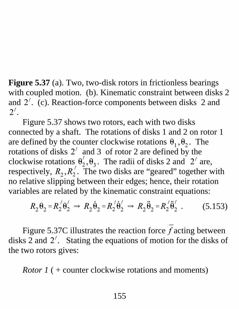
Figure 5.37 (a). Two, two-disk rotors in frictionless bearingswith coupled motion. (b). Kinematic constraint between disks 2and . (c). Reaction-force components between disks 2 and

.Figure 5.37 shows two rotors, each with two disks

connected by a shaft. The rotations of disks 1 and 2 on rotor 1are defined by the counter clockwise rotations . Therotations of disks and 3 of rotor 2 are defined by theclockwise rotations . The radii of disks 2 and are,respectively, . The two disks are “geared” together withno relative slipping between their edges; hence, their rotationvariables are related by the kinematic constraint equations:

Figure 5.37C illustrates the reaction force acting betweendisks 2 and . Stating the equations of motion for the disks ofthe two rotors gives:

Rotor 1 ( + counter clockwise rotations and moments)

156

(5.154a)

(5.154b)

Rotor 2 (+ clockwise rotations and moments)

Eqs.(5.153) and (5.154) comprise five equations in the fiveunknowns . Equating in the second ofEqs.(5.154a) and the first of Eqs.(5.154b) eliminates thisvariable. Also, Eq.(5.153) can be used to eliminate

yielding the following three coupled differentialequations:

These equations define a three-degree-of-freedom problem withthe matrix statement

157

(5.155)

Because neither of the component rotors are connected toground, one of the eigenvalues is zero, and the remaining tworoots (and their associated eigenvectors) can be determinedanalytically.

158

Lecture 33. BEAMS AS SPRINGS VIBRATION EXAMPLES

Unlike linear extension/compression springs that deliver areaction force opposing the direction of displacement, ortorsional springs that produces a reaction torque to opposetwisting, deflecting or rotating the end of a beam normallyproduce both a reaction moment and a reaction force. Thecoupling of displacements and rotations and reaction forces andmoments can be confusing, and we will start with a simpleexample of a cantilevered beam with an attached weight. Displacement of the beam’s end creates a reaction force but noreaction moment.

Figure 5.38 Lumped-parameter rotormodel including two disks.

159

Example A. Cantilever Beam supporting a disk that does notrotate. Zero moments about the right end. The bar has mass m. The beam has length l and section modulus EI.

If it is pulled down and then released (the cable remains intension), what is the natural frequency of free motion for thedisk?

Figure XP 5.2bCantilever beamwith the diskhanging from itsend.

From strength of materials, a beam with a zero moment at its freeend and a lateral load f will deflect a distance δ. δ and f arerelated by

In this equation, defines the displacement

“flexibility coefficient” for the beam’s end. We want thedisplacement stiffness coefficient (for zero moment at the beam’s

160

end)

For motion about the equilibrium position, the free-body diagramfor the disk (massless beam) is shown below. ( δ remains smallenough that the cord remains in tension.)

Free-body diagram.

From the free-body diagram, the equation of motion is,

and the natural frequency is

161

Suppose the beam has length and a circular crosssection with diameter . It is made from steel with

modulus of elasticity . The disk has radius , thickness and is also made from

steel (density ). As a first step, the bendingsection modulus is

The mass is

Substituting, the natural frequency is

162

where the dimensions of a kg are .

Figure 5.39a represents the more general situation with a diskrigidly attached to the end of a cantilevered beam. If the disk isdisplaced from its equilibrium position, the disk will rotate in theY-Z plane through the angle Because of the disk’s moment of

inertia, a moment will now result at the beam’s end due to diskrotation. Figure 5.39b provides the free-body diagram for thedisplaced and rotated disk, including the applied force andmoment pair and reaction force and moment pair

.

Figure 5.39

Cantilevered beamsupporting a thin circulardisk at its right end.

Free-body diagram for thedisk.

The equations of motion are easily stated from figure 5.39b . Applying and , the disk’s equations of

motion are:

163

(5.156)

(5.157a)

Defining the reaction force and moment in terms of the

displacement and rotation coordinates is the principal

difficulty in completing these equations.

Figure 5.40 (a). Cantileveredbeam with an applied end force. (b). Applied moment

Figure 5.40a illustrates the beam with a concentrated load applied at its end, yielding (from strength of materials) thedisplacement and rotation.

We used the displacement result in the first example. Similarly,figure 5.40b illustrates a moment M applied to the beam’s end,yielding

164

Combining these results as and

gives

In matrix format, these equations are

This coefficient matrix is a “flexibility” matrix . An

flexibility-matrix entry is the displacement (or rotation) at pointi due to a unit load (or moment) at point j . Multiplying throughby gives

165

(5.158)

(5.159)

(5.160)

This coefficient matrix is the stiffness matrix . Theform of this equation tends to be confusing if we think of it asdefining the applied loads as the output due to inputdisplacements and rotations . However, the following

statement makes sense when defining the reaction force andmoment of figure 5.39b due to displacements and rotations

Substituting this result into Eqs.(5.156) gives the matrix equationof motion,

or

166

(5.160)

An entry for the stiffness matrix is the negative reaction force

(or moment) at point i due to a displacement (or rotation) atstation j , with all other displacements and rotations equal tozero.

Example Problem 5.1 The cantilevered beam of figure 5.39 haslength , a circular cross section with diameter

. It is made from steel with modulus of elasticity

. The disk has radius ,thickness and is also made from steel (density =

). The following engineering-analysis tasksapply:

a. Determine the inertia and stiffness matrices and state thematrix equation of motion.

167

b. Determine the eigenvalues, natural frequencies, andeigenvectors.

Solution. As a first step, the bending section modulus is

Continuing, the stiffness coefficients are:

The inertia-matrix entries are:

168

(i)

(ii)

Substituting these results into Eq.(5.160) defines the model as

Substituting the solution into the

homogeneous version of Eq.(i) nets

The characteristic equation is

The eigenvalues and natural frequencies defined by the roots ofthis equation are:

169

(iii)

(iv)

The first natural frequency is slightly lower than

the initial example result

Substituting and into Eq.(ii), the corresponding

eigenvectors are:

As illustrated in figure XP 5.1a, the displacement and rotation

170

(5.160)

are in phase for the first mode and out of phase for the second.Figure XP 5.2a Calculated mode shapes of Eq.(iv); not to scale.

Figure XP 5.2c Cantilever beam with the end disk forced tomove up and down but prevented from rotating. .

The disk in Figure XP 5.2c is constrained by rollers that preventrotation. For , the example has only one degree of freedom

, and Eq.(5.160)

gives:

171

The first equation is the equation of motion for . The second

equation defines the reaction moment that the constraint rollersmust provide to keep the disk from rotating. The naturalfrequency is defined by

The moment restraint on the disk has doubled the lowest naturalfrequency.

Note that we have determined the displacement stiffness for acantilever beam whose end is deflected with zero rotation to be

172

Example Problem 5.5. The framed structure has two squarefloors. The first floor has mass and is supported to

the foundation by four solid columns with square cross sections. These columns are cantilevered from the foundation and arewelded to the bottom of the first floor. The second floor hasmass and is supported from the first floor by four

solid columns with square cross sections. These columns arewelded to the top of the first floor and are hinged to the secondfloor. The bottom and top columns have length and

. The top and bottom beams’ cross-sectional dimensions

are and . They are made from steel with

a modulus of elasticity . A model is requiredto account for motion of the foundation due to earthquakeexcitation defined by .

Tasks: a. Select coordinates, draw a free-body diagram, derive the

equations of motion.

b. State the equations of motion in matrix format and solvefor the eigenvalues and eigenvectors. Draw theeigenvectors.

173

Figure XP5.5 (a) Front view of a two-storyframed structure excited by base excitation,(b) Coordinates, (c) Free-body diagram for

, (d) Eigenvectors

174

Solution. Figure XP5.5 b illustrates the coordinates

selected to locate the first and second floors with respect toground. All beams connecting the foundation and the first floorare cantilevered at both ends, similar to the beam in figure 5.47with a stiffness . The free-body diagram of figure

XP5.5c was drawn assuming that the first floor has movedfurther than the ground and defines the reaction force

due to all four cantilevered beams acting at the bottom of floor 1.

Each beam connecting the floors has a cantilevered endattached to floor 1 and a pinned end attached to floor 2, similar tothe pinned-end beam of figure 5.44, with a stiffness coefficient

. The free-body diagram in figure XP5.5c was

developed assuming that the second floor has moved further thanthe first floor and provides

The negative of this force is acting at the top of floor 1. Summing forces for the two floors gives:

175

(i)

Putting these equations in matrix form gives

This outcome is similar to Eq.(3.126) for two masses connectedby springs.

Filling in the numbers gives:

176

(iii)

(ii)

Continuing, the stiffness coefficients are:

Plugging these results into Eq.(i) gives

Substituting the assumed solution into

the homogeneous version of this equation gives

Since, , and and are also not zero, a nontrivial

solution, for Eq.(ii) requires that the determinant of thecoefficient matrix must equal zero, producing

177

This characteristic equation defines the two eigenvalues andnatural frequencies:

Alternately substituting and

into Eq.(iii) gives the eigenvectors

Figure XP5.5d illustrates these two eigenvectors, showing therelative motion of the two floors somewhat better that the two-mass eigenvectors of figure 3.53.

178

Lecture 34. 2DOF EXAMPLES

Example 1

The cylinders roll without slipping. Select coordinates, drawfree-body diagrams, and derive the equations of motion.

Coordinates and free-body diagram for

k1 k2

k3 A

m, R

B

m, R

179

Equations of motion, cylinder 1

Equations of motion cylinder 2

Four equations, 6 unknowns

Rolling-without slipping kinematic constraints:

Eliminate in (1), and in (2)

(2)

(3)

(3)

180

Use (3) to eliminate , and rearrange

For and the matrix form is

181

Alternative development: Take moments about C the pointof contact

General moment equation for clockwise moments

However,

Hence,

182

Similarly for cylinder 2

Matrix Format

This is the same equation

183

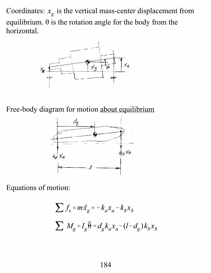
Example 2

Assume small rotations, select coordinates, draw free-bodydiagrams, and derive the equations of motion. Gravity isvertically down, and the body is in equilibrium.

d1

D1

kA

L1 L2

D2

kB

d2

D3 D3

P

Y

184

Coordinates: is the vertical mass-center displacement from

equilibrium. θ is the rotation angle for the body from thehorizontal.

Free-body diagram for motion about equilibrium

Equations of motion:

185

Small-angle kinematics:

Substituting,

Gathering terms,

Matrix Format

A good deal of effort is required on the homework problem toget and .

186

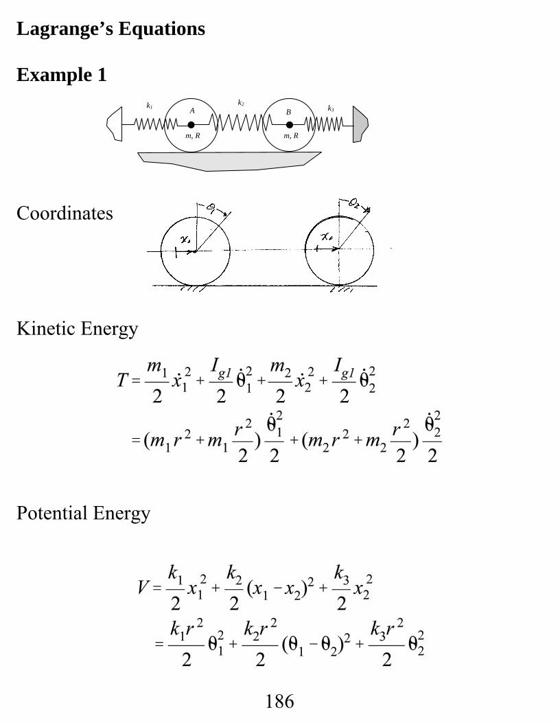
Lagrange’s Equations

Example 1

Coordinates

Kinetic Energy

Potential Energy

k1 k2

k3 A

m, R

B

m, R

187

Lagrangian

EOM

Result from

Example 2

188

Kinematics:

Proceeding

189

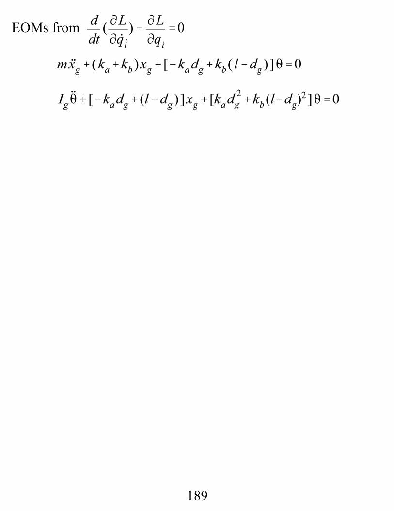
EOMs from

190

Lecture 35. More 2DOF EXAMPLESA Translating Mass with an Attached Compound Pendulum

Figure 5.53 Translating cart of mass Msupported by frictionless rollers andsupporting a compound pendulum oflength l and mass m . (a) Equilibriumposition, (b) General position (c) Cartfree-body diagram, (d) Pendulum free-body diagram.

191

(5.201)

(5.202)

Cart EOM

Pendulum Moment Equation

Moment about g:

will draw the unknown and unwanted reaction components into the moment equation.

Moment about o using

is quicker. An inspection of the pendulum in figure 5.53c gives:

Hence, stating the moment equation about the pivot point ogives

192

(5.203)

where We now have two equations (the first ofEq.(5.201) and Eq.(5.202)) for the three unknowns: .

The X component of the equation of the pendulumgives the last required EOM as

However, this equation introduces the new unknown , whichcan be eliminated, starting from the geometric relationship

Differentiating this equation twice with respect to time gives

Substituting for into Eq.(5.203) gives

Now, substituting this definition into the first of Eq.(5.201)gives

193

(5.204)

(5.205)

Eqs.(5.202) and (5.204) comprise the two governing equationsin . Their matrix statement is:

We have now completed Task a. Assuming “small” motion for this system means that second

order terms in X and θ are dropped. Introducing the small angleapproximations ; , and dropping second orderand higher terms in θ and yields:

194

(5.206)

which concludes Task b.

195

APPLYING LAGRANGE’S EQUATION OF MOTION TOEXAMPLES WITH GENERALIZED COORDINATES (NOKINEMATIC CONSTRAINTS).

Coupled Cart/Pendulum

Figure 6.3 Translating cart withan attached pendulum (no externalforce)

This system has the two coordinates X ,θ and two degrees offreedom. Hence, the two coordinates X ,θ are the generalizedcoordinates , and their derivatives are the generalizedvelocities of Lagrange’s equations. The followingengineering task applies: Use Lagrange’s equations to derivethe equations of motion.

196

(5.183)

The kinetic energy of the cart is easily calculated as.

The kinetic energy of the pendulum follows from the generalkinetic energy for planar motion of a rigid body

where is the velocity of the body’s mass center with respectto an inertial coordinate system. The pendulum’s mass center islocated by

Hence

and

Hence, the system kinetic energy is

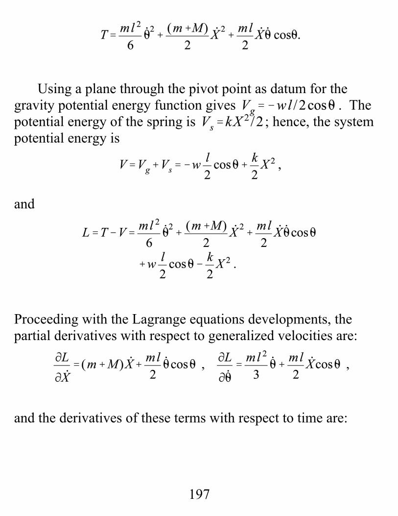
197

Using a plane through the pivot point as datum for thegravity potential energy function gives . Thepotential energy of the spring is ; hence, the systempotential energy is

and

Proceeding with the Lagrange equations developments, thepartial derivatives with respect to generalized velocities are:

and the derivatives of these terms with respect to time are:

198

(6.29)

Once again, note the last terms in these derivatives. The partial derivatives of L with respect to the generalized

coordinates are

By substitution, the governing equations of motion are:

The right-hand terms are zero, because there are nononconservative forces. Eqs.(6.29) are stated in matrix notationas

199

(6.30)

which coincides with Eq.(5.160) ( without the external force offigure 5.38) that we derived earlier from a free-bodydiagram/Newtonian approach. Again, the results are obtainedwithout recourse to free-body diagrams, and only velocities arerequired for the kinematics.

200

A Swinging Bar Supported at its End by a CordFigure 5.54a shows a swinging bar AB, supported by a cord

connecting end A to the support point O The cord has length l1 ;the bar has length l2 and mass m. This system has the twodegrees of freedom φ and θ. The engineering tasks for thissystem is: Derive the governing differential equations ofmotion.

Figure 5.54 Swinging bar supported at its end by a cord. (a)Equilibrium, (b) Coordinate choices, (c) Free-body diagram

From , the force component equations are:

201

(5.163)

The acceleration components can be obtained by stating thecomponents of Rg as:

Differentiating these equations twice with respect to time gives

Substitution gives

202

(5.165)

(5.164)

Eliminate Tc from these equations by: (i) multiply the first by, (ii) multiply the second by , and (iii) add the

results to obtain

This is the first of our required differential equations.One could reasonably state a moment equation about either

g , the mass center, or the end A. Stating the moment about Ahas the advantage of eliminating the reaction force , and wewill use the following version of the moment Eq.(5.24)

203

(5.166b)

(5.166a)

The moment due to the weight is negative because it actsopposite to the positive counterclockwise direction of θ. Thevector goes from A to g and is defined by

To complete Eq.(5.165), we need to define . The cord lengthis constant; hence, the radial acceleration component consists ofthe centrifugal-acceleration term . Similarly, thecircumferential acceleration term reduces to . Resolvingthese terms into their components along the X and Y axes gives

Figure 5.55 Polar kinematicsfor the cord to determine .

204

(5.167)

Eqs.(5.166) give

Substituting this result into Eq.(5.165) gives

This is the desired moment equation for the bar and is the secondand last equation of motion with . Eqs.(5.164) and(5.167) can be combined into the following matrix equation.

205

The inertia-coupling matrix can be made symmetric bymultiplying the top row by l1 . Eliminating second-order termsin θ and φ in this equation gives the linear vibration equations