Embed Size (px)
Citation preview
. . . . . .
Lecture 4: Covariance pattern models
Lecture 4: Covariance pattern models
Antonello Maruotti
Lecturer in Medical Statistics, S3RI and School of MathematicsUniversity of Southampton
Southampton, 13 June 2014
1 / 30
. . . . . .
Lecture 4: Covariance pattern models
Outline
Summary
Covariance structure for repeated measurements
Modelling growth curves
2 / 30
. . . . . .
Lecture 4: Covariance pattern models
Summary
Linear mixed models
I Statistical linear mixed models state that observed dataconsist of two parts
I fixed effectsI random effects
I Fixed effects define the expected values of the observations
I Random effects result from variation between subjects andfrom variation within subjects.
3 / 30
. . . . . .
Lecture 4: Covariance pattern models
Summary
Linear mixed models
I Measures on the same subject at different times almost alwaysare correlated, with measures taken close together in timebeing more highly correlated than measures take far apart intime
I Observations on different subjects are often assumeindependent
I Mixed linear models are used with repeated measures data toaccommodate the fixed effects of covariates and thecovariation between observations on the same subject atdifferent times
4 / 30
. . . . . .
Lecture 4: Covariance pattern models
Summary
Linear mixed models
I To model the mean structure in sufficient generality to ensureunbiasedness of the fixed effect estimates
I To specify a model for a covariance structure of the data
I Estimation methods are used to fit the mean portion of themodel
I The fixed effects portion may be made more parsimonious
I Statistical inference are drawn base on fitting this final model
5 / 30
. . . . . .
Lecture 4: Covariance pattern models
Covariance structure for repeated measurements
Model specification
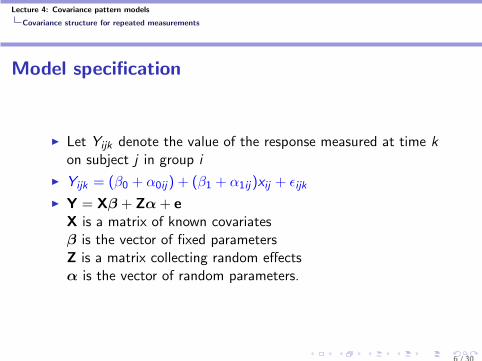
I Let Yijk denote the value of the response measured at time kon subject j in group i
I Yijk = (β0 + α0ij) + (β1 + α1ij)xij + ϵijkI Y = Xβ + Zα+ e
X is a matrix of known covariatesβ is the vector of fixed parametersZ is a matrix collecting random effectsα is the vector of random parameters.
6 / 30
. . . . . .
Lecture 4: Covariance pattern models
Covariance structure for repeated measurements
Covariance structure
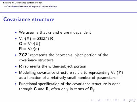
I We assume that α and e are independent
I Var(Y) = ZGZ’+RG = Var(U)R = Var(e)
I ZGZ’ represents the between-subject portion of thecovariance structure
I R represents the within-subject portion
I Modelling covariance structure refers to representing Var(Y)as a function of a relatively small number of parameters.
I Functional specification of the covariance structure is donethrough G and R, often only in terms of Rij
7 / 30
. . . . . .
Lecture 4: Covariance pattern models
Covariance structure for repeated measurements
Simple covariance structure
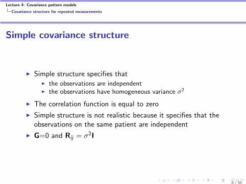
I Simple structure specifies thatI the observations are independentI the observations have homogeneous variance σ2
I The correlation function is equal to zero
I Simple structure is not realistic because it specifies that theobservations on the same patient are independent
I G=0 and Rij = σ2I
8 / 30
. . . . . .
Lecture 4: Covariance pattern models
Covariance structure for repeated measurements
Compound Symmetric or Exchangeable
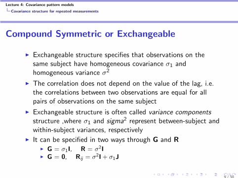
I Exchangeable structure specifies that observations on thesame subject have homogeneous covariance σ1 andhomogeneous variance σ2
I The correlation does not depend on the value of the lag, i.e.the correlations between two observations are equal for allpairs of observations on the same subject
I Exchangeable structure is often called variance componentsstructure ,where σ1 and sigma2 represent between-subject andwithin-subject variances, respectively
I It can be specified in two ways through G and RI G = σ1I, R = σ2II G = 0, Rij = σ2I+ σ1J
9 / 30
. . . . . .
Lecture 4: Covariance pattern models
Covariance structure for repeated measurements
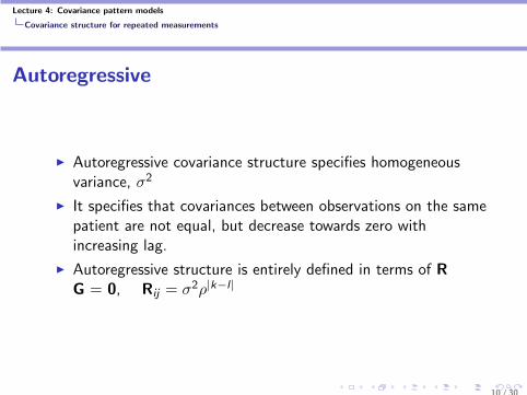
Autoregressive
I Autoregressive covariance structure specifies homogeneousvariance, σ2
I It specifies that covariances between observations on the samepatient are not equal, but decrease towards zero withincreasing lag.
I Autoregressive structure is entirely defined in terms of RG = 0, Rij = σ2ρ|k−l |
10 / 30
. . . . . .
Lecture 4: Covariance pattern models
Covariance structure for repeated measurements
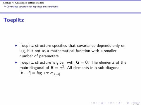
Toeplitz
I Toeplitz structure specifies that covariance depends only onlag, but not as a mathematical function with a smallernumber of parameters.
I Toeplitz structure is given with G = 0. The elements of themain diagonal of R = σ2. All elements in a sub-diagonal|k − l | = lag are σ|k−l |
11 / 30
. . . . . .
Lecture 4: Covariance pattern models
Covariance structure for repeated measurements
Unstructured
I The unstructured structure specifies no patterns in thecovariance matrix
I The covariance matrix is completely general
I A very large number of parameters need to be estimated
12 / 30
. . . . . .
Lecture 4: Covariance pattern models
Modelling growth curves
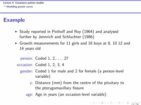
Example
I Study reported in Pothoff and Roy (1964) and analysedfurther by Jennrich and Schluchter (1986)
I Growth measurements for 11 girls and 16 boys at 8, 10 12 and14 years old
person: Coded 1, 2,. . . , 27
occasion: Coded 1, 2, 3, 4
gender: Coded 1 for male and 2 for female (a person-levelvariable)
y: Distance (mm) from the centre of the pituitary tothe pterygomaxillary fissure
age: Age in years (an occasion-level variable)
13 / 30
. . . . . .
Lecture 4: Covariance pattern models
Modelling growth curves
Statistical ModellingHow might we model growth?
I Assume independence between subjects, but expect repeatmeasurements on the same individual to be correlated
I Regard occasions as nested within subject
I Could formulate a linear mixed model utilising a randomcoefficients model
I An alternative formulation of the linear mixed model is tofocus on the:
I Marginal mean structure ⇒ Modelled using fixed effectsI Marginal covariance structure ⇒ Requiring a model for the
pattern of the covariance matrix associated with randomvariation between individual subject response vectors
I Known as a marginal model, or covariance pattern model ⇒response = fixed effects model for mean + random error
14 / 30
. . . . . .
Lecture 4: Covariance pattern models
Modelling growth curves
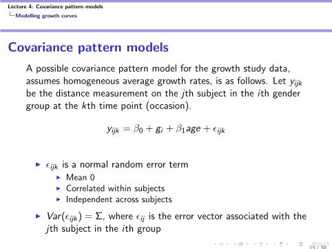
Covariance pattern models
A possible covariance pattern model for the growth study data,assumes homogeneous average growth rates, is as follows. Let yijkbe the distance measurement on the jth subject in the ith gendergroup at the kth time point (occasion).
yijk = β0 + gi + β1age + ϵijk
I ϵijk is a normal random error termI Mean 0I Correlated within subjectsI Independent across subjects
I Var(ϵijk) = Σ, where ϵij is the error vector associated with thejth subject in the ith group
15 / 30
. . . . . .
Lecture 4: Covariance pattern models
Modelling growth curves
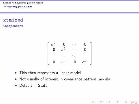
xtmixedindependent
σ2 0 · · · 00 σ2 · · · 0...
.... . .
...0 · · · 0 σ2
I This then represents a linear model
I Not usually of interest in covariance pattern models
I Default in Stata
16 / 30
. . . . . .
Lecture 4: Covariance pattern models
Modelling growth curves
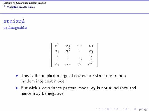
xtmixedexchangeable
σ2 σ1 · · · σ1σ1 σ2 · · · σ1...
.... . .
...σ1 · · · σ1 σ2
I This is the implied marginal covariance structure from a
random intercept model
I But with a covariance pattern model σ1 is not a variance andhence may be negative
17 / 30
. . . . . .
Lecture 4: Covariance pattern models
Modelling growth curves
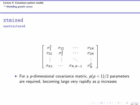
xtmixedunstructured
σ21 σ12 · · · σ1K
σ21 σ22 · · · σ2K
......
. . ....
σK1 · · · σK ,K−1 σ2K
I For a p-dimensional covariance matrix, p(p + 1)/2 parameters
are required, becoming large very rapidly as p increases
18 / 30
. . . . . .
Lecture 4: Covariance pattern models
Modelling growth curves
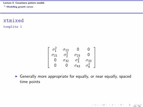
xtmixedtoeplitz 1
σ21 σ12 0 0
σ21 σ22 σ23 0
0 σ32 σ23 σ33
0 0 σ43 σ24
I Generally more appropriate for equally, or near equally, spaced
time points
19 / 30
. . . . . .
Lecture 4: Covariance pattern models
Modelling growth curves
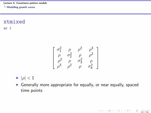
xtmixedar 1
σ21 ρ ρ2 ρ3
ρ σ22 ρ ρ2
ρ2 ρ σ23 ρ
ρ3 ρ2 ρ σ24
I |ρ| < 1
I Generally more appropriate for equally, or near equally, spacedtime points
20 / 30
. . . . . .
Lecture 4: Covariance pattern models
Modelling growth curves
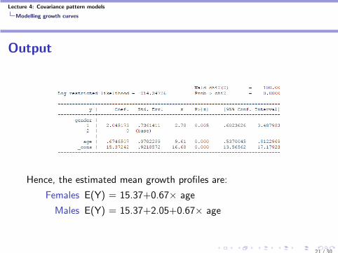
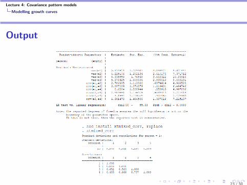
Output
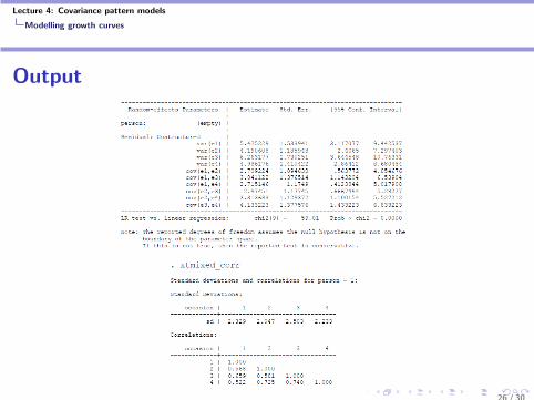
Hence, the estimated mean growth profiles are:
Females E(Y) = 15.37+0.67× age
Males E(Y) = 15.37+2.05+0.67× age
21 / 30
. . . . . .
Lecture 4: Covariance pattern models
Modelling growth curves
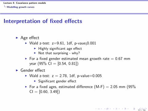
Interpretation of fixed effects
I Age effectI Wald z-test: z=9.61, 1df, p-vaue¡0.001
I Highly significant age effectI Not that surprising - why?
I For a fixed gender estimated mean growth rate = 0.67 mmyear (95% CI = [0.54, 0.81])
I Gender effectI Wald z-test: z = 2.78, 1df, p-value=0.005
I Significant gender effect
I For a fixed ages, estimated difference (M-F) = 2.05 mm (95%CI = [0.60, 3.49])
22 / 30
. . . . . .
Lecture 4: Covariance pattern models
Modelling growth curves
Output
23 / 30
. . . . . .
Lecture 4: Covariance pattern models
Modelling growth curves
Heterogeneous average growth rates
I Is there a significant interaction between gender and age?
I Add an interaction term into the previous model
yijk = β0 + gi + β1iage + ϵijk
24 / 30
. . . . . .
Lecture 4: Covariance pattern models
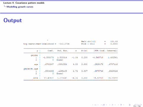
Modelling growth curves
Output
25 / 30
. . . . . .
Lecture 4: Covariance pattern models
Modelling growth curves
Output
26 / 30
. . . . . .
Lecture 4: Covariance pattern models
Modelling growth curves
Choice of covariance structure
I The previous analysis assumed an unstructured covariancematrix for ϵij
I From inspecting the estimated covariance matrix, Σ̂ , mightthere be a simpler covariance structure which is plausible?
I A more parsimonious covariance, if valid, is desirable forimproved precision and power
I An incorrect choice of covariance structure may lead toerroneous conclusions
I An unstructured covariance matrix is not necessarily correct.Why?
27 / 30
. . . . . .
Lecture 4: Covariance pattern models
Modelling growth curves
Choice of covariance structure
Different covariance structures may be compared:
I Descriptively
I Using a hypothesis test the likelihood ratio test, assuming ⇒Nested models
I Using information theoretic criteria AIC, BIC⇒ Useful forcomparing non-nested models
28 / 30
. . . . . .
Lecture 4: Covariance pattern models
Modelling growth curves
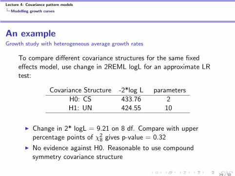
An exampleGrowth study with heterogeneous average growth rates
To compare different covariance structures for the same fixedeffects model, use change in 2REML logL for an approximate LRtest:
Covariance Structure -2*log L parameters
H0: CS 433.76 2H1: UN 424.55 10
I Change in 2* logL = 9.21 on 8 df. Compare with upperpercentage points of χ2
8 gives p-value = 0.32
I No evidence against H0. Reasonable to use compoundsymmetry covariance structure
29 / 30
. . . . . .
Lecture 4: Covariance pattern models
Modelling growth curves
Final remarks
I Covariance pattern models are useful when primary interest isin modelling the mean structure
I Offers a flexible modelling approachI Different covariance structures are permissibleI Allows for subjects with missing valuesI Time dependent explanatory variables
I Covariance pattern models are essentially linear models,allowing for correlated errors and heterogeneous variance
30 / 30