Lecture 5: Matrix Volume

1

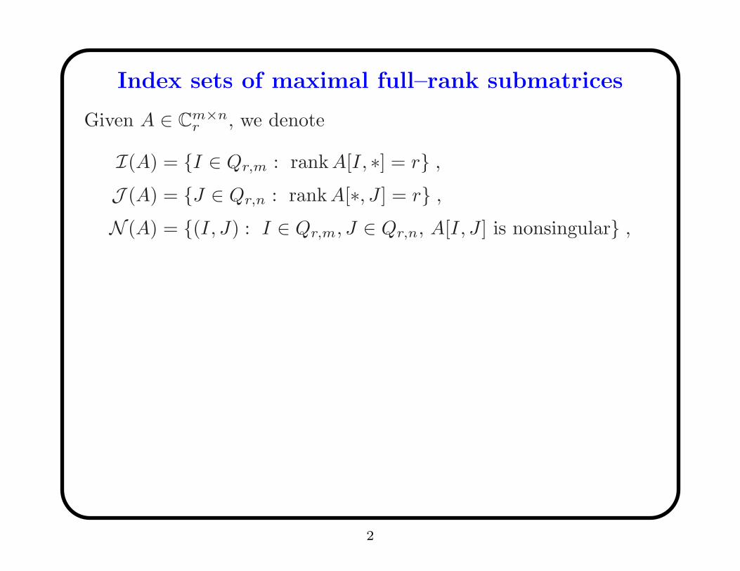
Index sets of maximal full–rank submatrices

Given A ∈ Cm×nr , we denote

I(A) = {I ∈ Qr,m : rank A[I, ∗] = r} ,

J (A) = {J ∈ Qr,n : rank A[∗, J ] = r} ,

N (A) = {(I, J) : I ∈ Qr,m, J ∈ Qr,n, A[I, J ] is nonsingular} ,

2

Index sets of maximal full–rank submatrices

Given A ∈ Cm×nr , we denote

I(A) = {I ∈ Qr,m : rank A[I, ∗] = r} ,

J (A) = {J ∈ Qr,n : rank A[∗, J ] = r} ,

N (A) = {(I, J) : I ∈ Qr,m, J ∈ Qr,n, A[I, J ] is nonsingular} ,

If

A = CR

is a full rank factorization, then

I(A) = I(C)

J (A) = J (R)

N (A) = I(A) × J (A)

Note: I ∈ I(A) and J ∈ J (A) =⇒ A[I, J ] nonsingular (!?)

2-a

The Gramian

The Gram matrix of a set S = {x1,x2, . . . ,xk} ⊂ Rn is the k × k

matrix G(S), or G(x1,x2, . . . ,xk), of inner products

G(x1,x2, . . . ,xk)[i, j] := 〈xi,xj〉 .

det G(x1,x2, . . . ,xk) is the Gramian of {x1,x2, . . . ,xk}.If {x1,x2, . . . ,xk} are columns of X ∈ Rn×k, then

det G(x1, . . . ,xn) = detXT X =∑

I∈Qk,n

det2 XI∗ , (by C–B)

3

The Gramian

The Gram matrix of a set S = {x1,x2, . . . ,xk} ⊂ Rn is the k × k

matrix G(S), or G(x1,x2, . . . ,xk), of inner products

G(x1,x2, . . . ,xk)[i, j] := 〈xi,xj〉 .

det G(x1,x2, . . . ,xk) is the Gramian of {x1,x2, . . . ,xk}.If {x1,x2, . . . ,xk} are columns of X ∈ Rn×k, then

det G(x1, . . . ,xn) = detXT X =∑

I∈Qk,n

det2 XI∗ , (by C–B)

(a) The set S is linearly dependent iff G(S) = 0.

(b) The volume of the parallelepiped generated by the vectors

{x1,x2, . . . ,xk} is

vol � {x1,x2, . . . ,xk} =√

det G(x1,x2, . . . ,xk)

(in the subspace span {x1,x2, . . . ,xk}, not in Rn if k < n)

3-a

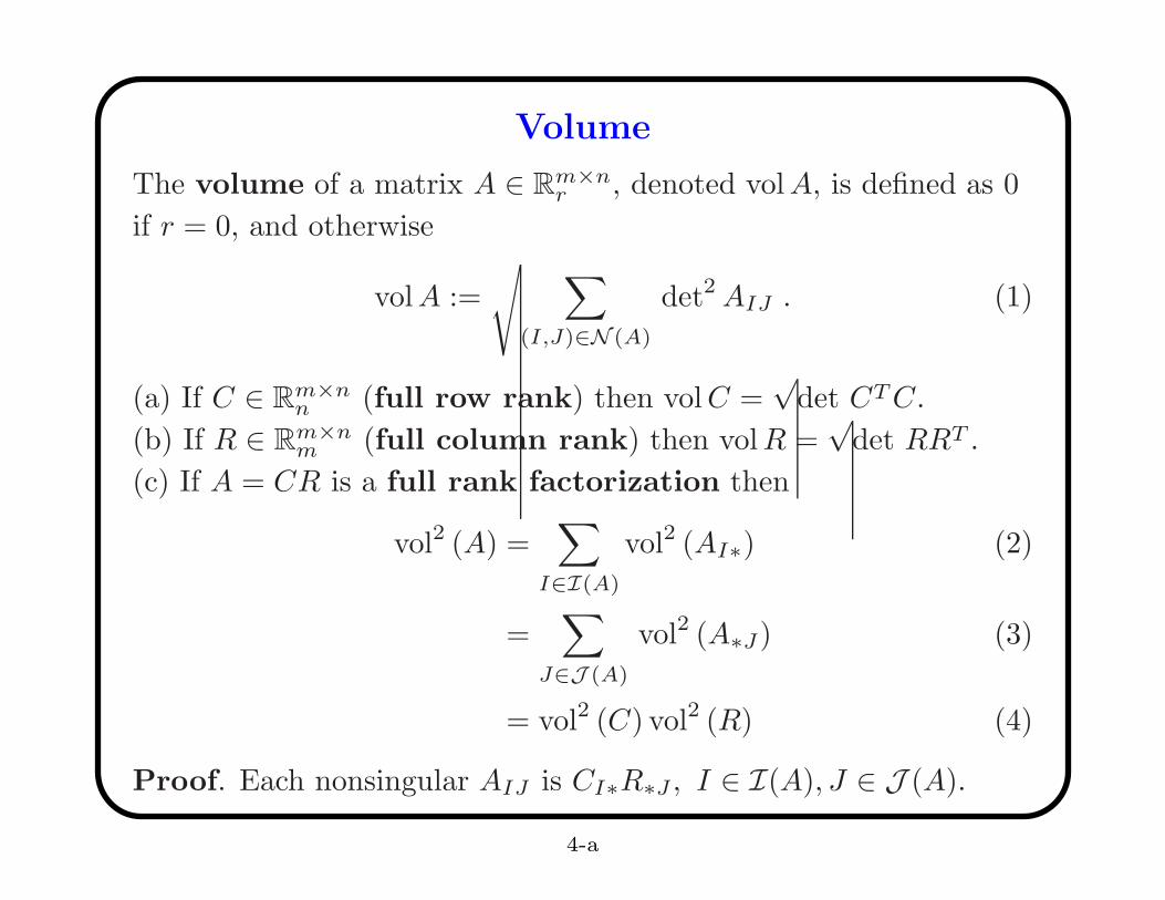
Volume

The volume of a matrix A ∈ Rm×nr , denoted vol A, is defined as 0

if r = 0, and otherwise

volA :=

√

∑

(I,J)∈N (A)

det2 AIJ . (1)

4

Volume

The volume of a matrix A ∈ Rm×nr , denoted vol A, is defined as 0

if r = 0, and otherwise

volA :=

√

∑

(I,J)∈N (A)

det2 AIJ . (1)

(a) If C ∈ Rm×nn (full row rank) then vol C =

√det CT C.

(b) If R ∈ Rm×nm (full column rank) then vol R =

√det RRT .

(c) If A = CR is a full rank factorization then

vol2 (A) =∑

I∈I(A)

vol2 (AI∗) (2)

=∑

J∈J (A)

vol2 (A∗J) (3)

= vol2 (C) vol2 (R) (4)

Proof. Each nonsingular AIJ is CI∗R∗J , I ∈ I(A), J ∈ J (A).

4-a

Singular values

Theorem. The volume of A ∈ Rm×nr is the product of its

singular values {σ1, · · · , σr}

vol A =∏

σi∈σ(A)

σi (1)

Proof. The SVD of A,

A = UΣV ∗ =[

U1 U2

]

Σ11 O

O O

V ∗1

V ∗2

, Σ11 ∈ Rr×rr ,

is a full rank factorization

A = U1Σ11V∗1 , with U∗

1 U1 = V ∗1 V1 = Ir .

∴ vol A = volΣ11 =∏

σi∈σ(A)

σi

5

Why ”volume”?

Let {vj : j ∈ 1, r} be an o.n. basis of R(A∗A) = R(A∗) such that

A∗Avj = σ2i vj , j ∈ 1, r ,

Then an o.n. basis {uj : j ∈ 1, r} of R(A) is given by

Avj = σj uj

showing that A maps the unit cube � {v1,v2, · · · ,vr} into the

cube � {σ1u1, σ2u2, · · · , σrur} of volume σ1σ2 · · ·σr. But the

singular values are orthogonally invariant, and therefore every

unit cube in R(A∗) is mapped into a cube of volume σ1σ2 · · ·σr.

Given A ∈ Rm×n, the volume of A is an intrinsic property of

the linear transformation in L(Rn, Rm) represented by A.

6

LSS

Let A ∈ Rm×nn , b ∈ Rm. Then the LSS of Ax = b is

A†b =∑

I∈I(A)

λIA−1I∗ bI , λI =

det2 AI∗∑

K∈I(A)

det2 AK∗

Ex. n = 1.

a1

...

am

x =

b1

...

bm

.

The LSS is

x =

m∑

i=1

aibi

m∑

k=1

a2k

=

m∑

i=1

a2i

m∑

k=1

a2k

a−1i bi =

m∑

i=1

λi a−1i bi

This trivial example proves the general case.

7

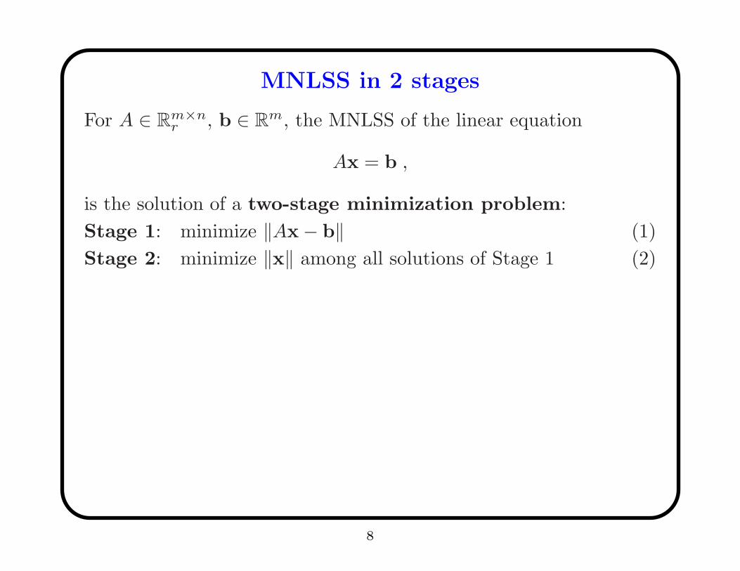
MNLSS in 2 stages

For A ∈ Rm×nr , b ∈ Rm, the MNLSS of the linear equation

Ax = b ,

is the solution of a two-stage minimization problem:

Stage 1: minimize ‖Ax − b‖ (1)

Stage 2: minimize ‖x‖ among all solutions of Stage 1 (2)

8

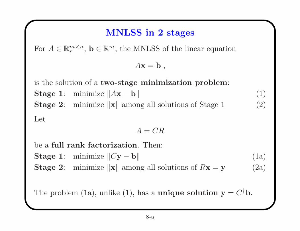
MNLSS in 2 stages

For A ∈ Rm×nr , b ∈ Rm, the MNLSS of the linear equation

Ax = b ,

is the solution of a two-stage minimization problem:

Stage 1: minimize ‖Ax − b‖ (1)

Stage 2: minimize ‖x‖ among all solutions of Stage 1 (2)

Let

A = CR

be a full rank factorization. Then:

Stage 1: minimize ‖Cy − b‖ (1a)

Stage 2: minimize ‖x‖ among all solutions of Rx = y (2a)

The problem (1a), unlike (1), has a unique solution y = C†b.

8-a

Full rank systems

Lemma.

(a) Let C ∈ Rm×rr , b ∈ Rm. Then the LSS of

Cy = b , (1)

is

y =∑

I∈I(C)

µI∗ C−1I∗ bI , µI∗ =

vol2CI∗vol2C

. (2)

9

Full rank systems

Lemma.

(a) Let C ∈ Rm×rr , b ∈ Rm. Then the LSS of

Cy = b , (1)

is

y =∑

I∈I(C)

µI∗ C−1I∗ bI , µI∗ =

vol2CI∗vol2C

. (2)

(b) Let R ∈ Rr×nr , y ∈ Rr. Then the MNS of

Rx = y , (3)

is

x =∑

J∈J (R)

ν∗JR−1∗J y , ν∗J =

vol2R∗J

vol2R. (4)

9-a

MNLSS as convex combination

Theorem (Berg). Let A ∈ Rm×nr , b ∈ Rm. Then the MNLSS of

Ax = b , (1)

is the convex combination

x =∑

(I,J)∈N (A)

λIJA−1IJ bI , (2)

with weights given by

λIJ =det2AIJ

∑

(K,L)∈N (A)

det2AKL

, (I, J) ∈ N (A) . (3)

Proof. Let A = CR be a full rank factorization, and use previous

lemma and the fact

AIJ = CI∗R∗J , ∀ I ∈ I(A), J ∈ J (A) .

10

Weighted LS

Consider next a weighted least squares problem

min ‖D1/2(Ax − b)‖ , D = diag (di) , di > 0 . (1)

Theorem (Ben–Tal and Teboulle). The solutions of (1), i.e.,

the least–squares solutions of D1/2Ax = D1/2b, satisfy the normal

equation, AT DAx = AT Db . The MN (weighted) LSS is

x(D) =∑

(I,J)∈N (A)

λIJ (D) A−1IJ bI , (2)

with weights

λIJ (D) =(∏

i∈I di) det2AIJ∑

(I,J)∈N (A)

(∏

i∈K di) det2AKL

. (3)

Note: Only the weights λIJ depend on D.

11

Bordered matrices

Let A ∈ Rm×nr , and let

U ∈ Rm×(m−r) , colsU = o.n. basisN(AT ) ,

V ∈ Rn×(n−r) , colsV = o.n. basisN(A) .

Consider the bordered matrix,

B(A) :=

A U

V T O

, (1)

and if m = n, the complemented matrix,

C(A) := A + UV T . (2)

Then

volA = |detB(A)| , (3)

= |detC(A)| . (4)

12

The change-of-variables formula in integration

Theorem (Jacobi general n, Euler n = 2, Lagrange n = 3)∫

Vf(v) dv =

∫

U(f ◦ φ)(u) |detJφ(u)| du (1)

13

The change-of-variables formula in integration

Theorem (Jacobi general n, Euler n = 2, Lagrange n = 3)∫

Vf(v) dv =

∫

U(f ◦ φ)(u) |detJφ(u)| du (1)

U ,V sets in Rn,

φ : U → V a sufficiently well-behaved function,

f is integrable on V ,

dx denotes the volume element | dx1 ∧ dx2 ∧ · · · ∧ dxn|,Jφ is the Jacobian matrix (or Jacobian)

Jφ :=

(

∂φi

∂uj

)

, also denoted∂(v1, v2, · · · , vn)

∂(u1, u2, · · · , un), (2)

representing the derivative of φ.

An advantage of (1) is that integration on V is translated to

(perhaps simpler) integration on U .

13-a

The change-of-variable formula (cont’d)

∫

Vf(v) dv =

∫

U(f ◦ φ)(u) |detJφ(u)| du (1)

If U ⊂ Rn and V ⊂ Rm with n > m, formula (1) cannot be applied.

14

The change-of-variable formula (cont’d)

∫

Vf(v) dv =

∫

U(f ◦ φ)(u) |detJφ(u)| du (1)

If U ⊂ Rn and V ⊂ Rm with n > m, formula (1) cannot be applied.

However, if the Jacobian Jφ is of full column rank throughout U ,

we can replace |detJφ| by the volume vol Jφ of the Jacobian to

get∫

Vf(v) dv =

∫

U(f ◦ φ)(u) volJφ(u) du . (2)

Here,

volJφ =√

det (JTφ Jφ) (3)

since Jφ is assumed of full rank, and (2) reduces to (1) if m = n.

14-a

Example in surface integration

Let S be a subset of a surface in R3 represented by

z = g(x, y) , (1)

and let f(x, y, z) be a function integrable on S. Let A be the

projection of S on the xy–plane. Then

S = φ(A) , or

xyz

=

xy

g(x, y)

= φ

[

xy

]

,

[

xy

]

∈ A . (2)

The Jacobi matrix of φ is the 3 × 2 matrix

Jφ(x, y) =∂(x, y, z)

∂(x, y)=

1 00 1gx gy

, (3)

where gx =∂g

∂x, gy =

∂g

∂y.

15

Example (cont’d)

vol Jφ = vol

1 00 1gx gy

=√

1 + g2x + g2

y . (4)

∴

∫

S

f(x, y, z) ds =

∫

A

f(x, y, g(x, y))√

1 + g2x + g2

y dx dy .

16

Example (cont’d)

vol Jφ = vol

1 00 1gx gy

=√

1 + g2x + g2

y . (4)

∴

∫

S

f(x, y, z) ds =

∫

A

f(x, y, g(x, y))√

1 + g2x + g2

y dx dy .

A

S

16-a

Cylindrical coordinates

Let S be a surface in R3, represented by

z = z(r, θ)

where r, θ are cylindrical coordinates,

x = r cos θy = r sin θz = z(r, θ)

17

Cylindrical coordinates

Let S be a surface in R3, represented by

z = z(r, θ)

where r, θ are cylindrical coordinates,

x = r cos θy = r sin θz = z(r, θ)

The Jacobi matrix is

Jφ =∂(x, y, z)

∂(r, θ)=

cos θ −r sin θsin θ r cos θ

∂z∂r

∂z∂θ

and its volume is

vol Jφ =

√

r2 + r2

(

∂z

∂r

)2

+

(

∂z

∂θ

)2

= r

√

1 +

(

∂z

∂r

)2

+1

r2

(

∂z

∂θ

)2

17-a

Cylindrical coordinates (cont’d)

An integral over a domain V ⊂ S is∫

Vf(x, y, z) dV =

∫

Uf(r cos θ, r sin θ, z(r, θ)) volJφ(r, θ) dr dθ

18

Cylindrical coordinates (cont’d)

An integral over a domain V ⊂ S is∫

Vf(x, y, z) dV =

∫

Uf(r cos θ, r sin θ, z(r, θ)) volJφ(r, θ) dr dθ

If S is symmetric about the z–axis, then

∂z

∂θ= 0 , i.e. z = z(r),

and∫

Vf(x, y, z) dV =

∫

Uf(r cos θ, r sin θ, z(r)) r

√

1 + z′(r)2 dr dθ

18-a

Surface integral in Rn

Let x = (xi), and x[1, k] := {(xi) : i ∈ 1, k}.A surface S in Rn is given by given by

xn := g(x1, · · · , xn−1) = g(x[1, (n − 1)]) , (1)

Let

V ⊂ S, f integrable on V , and it is required to calculate∫

Vf(x) dS (2)

U the projection of V on Rn−1, the space of variables x[1 : (n− 1)],

φ : U → V , the mapping given by its components

φ := (φ1, φ2, . . . , φn) ,

φi(x[1, (n − 1)]) := xi , i = 1, . . . , n − 1

φn(x[1, (n − 1)]) := g(x[1, (n − 1)])

19

Surface integral in Rn (cont’d)

The Jacobi matrix of φ is

Jφ =

1 0 · · · 0 00 1 · · · 0 0

0 0. . . 0 0

0 0 · · · 1 00 0 · · · 0 1∂g

∂x1

∂g

∂x2· · · ∂g

∂xn−2

∂g

∂xn−1

and its volume is

vol Jφ =

√

√

√

√1 +

n−1∑

i=1

(

∂g∂xi

)2

∴

∫

V

f(x) dS =

∫

U

f(x[1, (n − 1)], g(x[1, (n − 1)])) volJφ dx1 · · · dxn−1

20

Radon transform

Let Hξ,p be a hyperplane in Rn represented by

Hξ,p :=

{

x ∈ Rn :

n∑

i=1

ξi xi = p

}

= {x : <ξ,x>= p} (1)

where the normal vector ξ = (ξ1, · · · , ξn) of Hξ,p has ξn 6= 0.

Then Hξ,p is given as

Hξ,p = φ(Rn−1) (2)

with

φi(x[1, (n − 1)]) := xi , i ∈ 1, (n − 1)

φn(x[1, (n − 1)]) :=p

ξn−

n−1∑

i=1

ξi

ξnxi (3)

21

Radon transform (cont’d)

The volume of Jφ is here

volJφ =

√

√

√

√1 +n−1∑

i=1

(

ξi

ξn

)2

=‖ξ‖|ξn|

(4)

The Radon transform (Rf)(ξ, p) of a function f : Rn → R is its

integral over the hyperplane Hξ,p,

(Rf)(ξ, p) :=

∫

{x: <ξ,x> = p}

f(x) dx . (5)

The Radon transform can be computed as an integral in Rn−1

(Rf)(ξ, p) =‖ξ‖|ξn|

∫

Rn−1

f

(

x[1, (n − 1)],p

ξn−

n−1∑

i=1

ξi

ξnxi

)

dx1 · · · dxn−1 .

(6)

22

Integrals over Rn

Consider an integral over Rn,∫

Rn

f(x) dx =

∫

Rn

f(x1, x2, · · · , xn) dx1 · · · dxn (1)

Since Rn is a union of (parallel) hyperplanes,

Rn =

∞⋃

p=−∞{x : <ξ,x>= p} , where ξ 6= 0 , (2)

Compute (1) iteratively: an integral over Rn−1 (Radon

transform), followed by an integral on R,

∫

Rn

f(x) dx =

∞∫

−∞

dp

‖ξ‖ (Rf)(ξ, p) (3)

23

Integrals over Rn (cont’d)

∫

Rn

f(x) dx =

∞∫

−∞

dp

‖ξ‖ (Rf)(ξ, p) (3)

Here dp/‖ξ‖ is the differential of the distance along ξ (i.e. dp

times the distance between the parallel hyperplanes Hξ,p and

Hξ,p+1).

Then by the result for the Radon transform,∫

Rn

f(x) dx =

1

|ξn|

∞∫

−∞

∫

Rn−1

f

(

x[1, (n − 1)],p

ξn−

n−1∑

i=1

ξi

ξnxi

)

dx1 · · · dxn−1

dp .

(4)

24

Application in Probability

Let X = (X1, · · · ,Xn) have joint density fX(x1, · · · , xn) and let

y = h(x1, · · · , xn) (1)

where h : Rn → R is sufficiently well-behaved, in particular

∂h

∂xn6= 0,

and (1) can be solved for xn,

xn = h−1(y|x1, · · · , xn−1) (2)

with x1, · · · , xn−1 as parameters.

It is required to find the density fY(y) of Y.

25

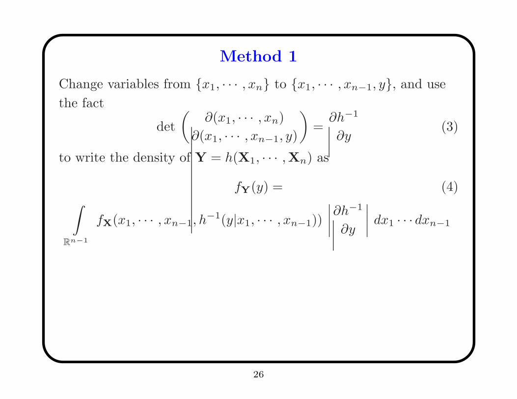
Method 1

Change variables from {x1, · · · , xn} to {x1, · · · , xn−1, y}, and use

the fact

det

(

∂(x1, · · · , xn)

∂(x1, · · · , xn−1, y)

)

=∂h−1

∂y(3)

to write the density of Y = h(X1, · · · ,Xn) as

fY(y) = (4)∫

Rn−1

fX(x1, · · · , xn−1, h−1(y|x1, · · · , xn−1))

∣

∣

∣

∣

∂h−1

∂y

∣

∣

∣

∣

dx1 · · · dxn−1

26

Method 2

Let V(y) be the surface given by (1), represented as

x1...xn−1

xn

=

x1...xn−1

h−1(y|x1, · · · , xn−1)

= φ

x1...xn−1

(5)

Then the surface integral of fX over V(y) is∫

V(y)

fX = (6)

∫

Rn−1

fX(x1, · · · , xn−1, h−1(y|x1, · · · , xn−1))

√

√

√

√1 +n−1∑

i=1

(

∂h−1

∂xi

)2

dx1 · · · dxn−1

27

The density of Y = h(X1, · · · ,Xn)

Theorem. If the ratio

∂h−1

∂y√

1 +n−1∑

i=1

(

∂h−1

∂xi

)2does not depend on x1, · · · , xn−1 , (X)

then

fY(y) =

∣

∣

∣

∂h−1

∂y

∣

∣

∣

√

1 +n−1∑

i=1

(

∂h−1

∂xi

)2

∫

V(y)

fX

Proof. Compare (4) and (6).

28

Hyperplanes

Condition (X) holds for hyperplanes. Let

y = h(x1, · · · , xn) :=n∑

i=1

ξi xi

where ξ = (ξ1, · · · , ξn) is a given vector with ξn 6= 0. Then (2) is

xn = h−1(y|x1, · · · , xn−1) :=y

ξn−

n−1∑

i=1

ξi

ξnxi

and∂h−1

∂y=

1

ξn,

√

√

√

√1 +

n−1∑

i=1

(

∂h−1

∂xi

)2

=

√

√

√

√1 +

n−1∑

i=1

(

ξi

ξn

)2

=‖ξ‖|ξn|

29

Hyperplanes (cont’d)

Corollary. Let X = (X1,X2, · · · ,Xn) be random variables with

joint density fX(x1, x2, · · · , xn), and let 0 6= ξ ∈ Rn.

The random variable

Y :=n∑

i=1

ξi Xi

has the density

fY(y) =(RfX)(ξ, y)

‖ξ‖ .

where (RfX)(ξ, y) is the Radon transform of fX,

(RfX)(ξ, y) =

‖ξ‖|ξn|

∫

Rn−1

fX

(

x1, · · · , xn−1,y

ξn−

n−1∑

i=1

ξi

ξnxi

)

dx1dx2 · · · dxn−1 .

30

Spheres

Condition (X) holds for spheres. Let

y = h(x1, · · · , xn) :=n∑

i=1

x2i

which has two solutions for xn, representing the upper and lower

hemispheres,

xn = h−1(y|x1, · · · , xn−1) := ±

√

√

√

√y −n−1∑

i=1

x2i

with∂h−1

∂y= ± 1

2√

y −∑n−1i=1 x2

i

,

√

√

√

√1 +n−1∑

i=1

(

∂h−1

∂xi

)2

=

√y

√

y −∑n−1i=1 x2

i

31

Spheres (cont’d)

Corollary. Let X = (X1, · · · ,Xn) have joint density

fX(x1, · · · , xn). The density of

Y =n∑

i=1

X2i

is

fY(y) =1

2√

y

∫

Sn(√

y)

fX

where the integral is over the sphere Sn(√

y) of radius√

y,

32

Spheres (cont’d)

computed as an integral over the ball Bn−1(√

y),

∫

Sn(√

y)

fX =

∫

Bn−1(√

y)

fX

x1, · · · , xn−1,

√

√

√

√y −n−1∑

i=1

x2i

+

+ fX

x1, · · · , xn−1,−

√

√

√

√y −n−1∑

i=1

x2i

√y dx1 · · · dxn−1√

y −∑n−1i=1 x2

i

33