Lecture 5: Search I · · 2018-03-27A farmer wants to get his cabbage , goat , and wolf across a ... Now we will proceed to the rst type of state-based models, search problems

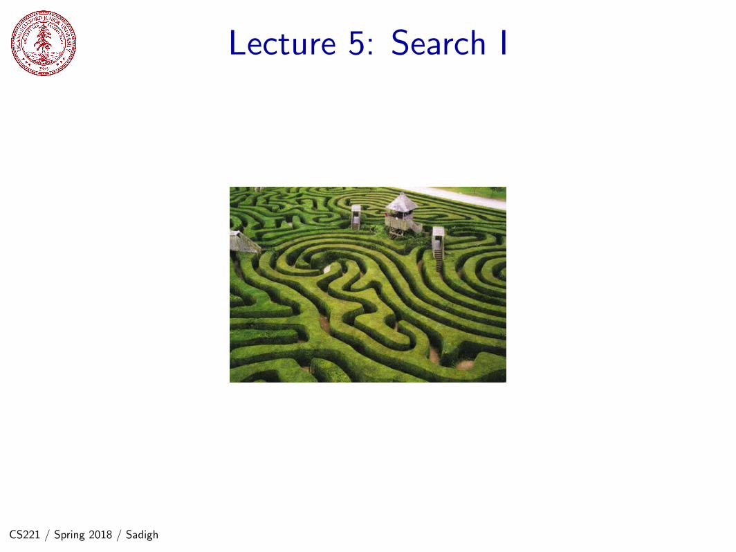
Lecture 5: Search I

CS221 / Spring 2018 / Sadigh

Question

A farmer wants to get his cabbage, goat, and wolf across a river. Hehas a boat that only holds two. He cannot leave the cabbage and goatalone or the goat and wolf alone. How many river crossings does heneed?

4

5

6

7

no solution

cs221.stanford.edu/q

CS221 / Spring 2018 / Sadigh 1

• When you solve this problem, try to think about how you did it. You probably simulated the scenario inyour head, trying to send the farmer over with the goat and observing the consequences. If nothing goteaten, you might continue with the next action. Otherwise, you undo that move and try something else.

• But the point is not for you to be able to solve this one problem manually. The real question is: Howcan we get a machine to do solve all problems like this automatically? One of the things we need isa systematic approach that considers all the possibilities. We will see that search problems define thepossibilities, and search algorithms explore these possibilities.


• This example, taken from xkcd, points out the cautionary tale that sometimes you can do better if youchange the model (perhaps the value of having a wolf is zero) instead of focusing on the algorithm.

Course plan

Reflex

Search problems

Markov decision processes

Adversarial games

States

Constraint satisfaction problems

Bayesian networks

Variables Logic

”Low-level intelligence” ”High-level intelligence”

Machine learning


• So far, we have worked with only the simplest types of models — reflex models. We used these as astarting point to explore machine learning. Now we will proceed to the first type of state-based models,search problems.

Paradigm

Modeling

Inference Learning


• Recall the modeling-inference-learning paradigm. For reflex-based classifiers, modeling consisted of choos-ing the features and the neural network architecture; inference was trivial forward computation of theoutput given the input; and learning involved using stochastic gradient descent on the gradient of the lossfunction, which might involve backpropagation.

• Today, we will focus on the modeling and inference part of search problems. The next lecture will coverlearning.

Application: route finding

Objective: shortest? fastest? most scenic?

Actions: go straight, turn left, turn right


• Route finding is perhaps the most canonical example of a search problem. We are given as the input amap, a source point and a destination point. The goal is to output a sequence of actions (e.g., go straight,turn left, or turn right) that will take us from the source to the destination.

• We might evaluate action sequences based on an objective (distance, time, or pleasantness).

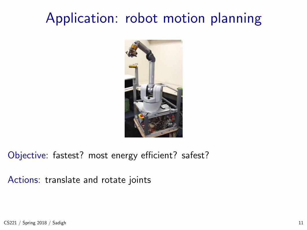
Application: robot motion planning

Objective: fastest? most energy efficient? safest?

Actions: translate and rotate joints


• In robot motion planning, the goal is get a robot to move from one position/pose to another. The desiredoutput trajectory consists of individual actions, each action corresponding to moving or rotating the jointsby a small amount.

• Again, we might evaluate action sequences based on various resources like time or energy.

Application: solving puzzles

Objective: reach a certain configuration

Actions: move pieces (e.g., Move12Down)


• In solving various puzzles, the output solution can be represented by a sequence of individual actions. Inthe Rubik’s cube, an action is rotating one slice of the cube. In the 15-puzzle, an action is moving onesquare to an adjacent free square.

• In puzzles, even finding one solution might be an accomplishment. The more ambitious might want tofind the best solution (say, minimize the number of moves).

Application: machine translation

la maison bleue

the blue house

Objective: fluent English and preserves meaning

Actions: append single words (e.g., the)


• In machine translation, the goal is to output a sentence that’s the translation of the given input sentence.The output sentence can be built out of actions, each action appending a word or a phrase to the currentoutput.

Beyond reflex

Classifier (reflex-based models):

x f single action y ∈ {−1,+1}

Search problem (state-based models):

x f action sequence (a1, a2, a3, a4, . . . )

Key: need to consider future consequences of an action!


• Last week, we finished our tour of machine learning of reflex-based models (e.g., linear predictors andneural networks) that output either a +1 or −1 (for binary classification) or a real number (for regression).

• While reflex-based models were appropriate for some applications such as sentiment classification or spamfiltering, the applications we will look at today, such as solving puzzles, demand more.

• To tackle these new problems, we will introduce search problems, our first instance of a state-basedmodel.

• In a search problem, in a sense, we are still building a predictor f which takes an input x, but f will nowreturn an entire action sequence, not just a single action. Of course you should object: can’t I just applya reflex model iteratively to generate a sequence? While that is true, the search problems that we’re tryingto solve importantly require reasoning about the consequences of the entire action sequence, and cannotbe tackled by myopically predicting one action at a time.

• Tangent: Of course, saying ”cannot” is a bit strong, since sometimes a search problem can be solved by areflex-based model. You could have a massive lookup table that told you what the best action to take forany given situation. .It is interesting to think of this as a time/memory tradeoff where reflex-based modelsare performing an implicit kind of caching. Going on a further tangent, one can even imagine compilinga state-based model into a reflex-based model; if you’re walking around Stanford for the first time, youmight have to really plan things out, but eventually it kind of becomes reflex.

• We have looked at many real-world examples of this paradigm. For each example, the key is to decomposethe output solution into a sequence of primitive actions. In addition, we need to think about how toevaluate different possible outputs.

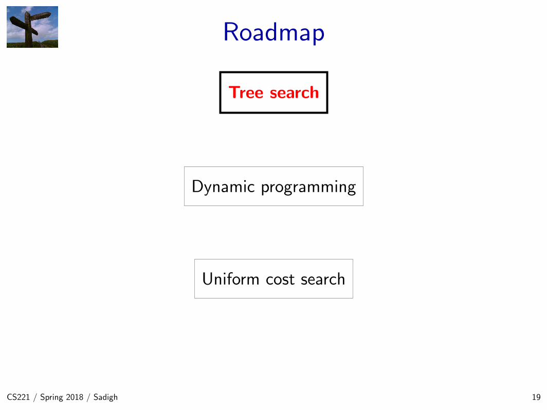
Roadmap

Tree search

Dynamic programming

Uniform cost search


Farmer Cabbage Goat Wolf

Actions:

F.

FC.

FG.

FW.

F/

FC/

FG/

FW/

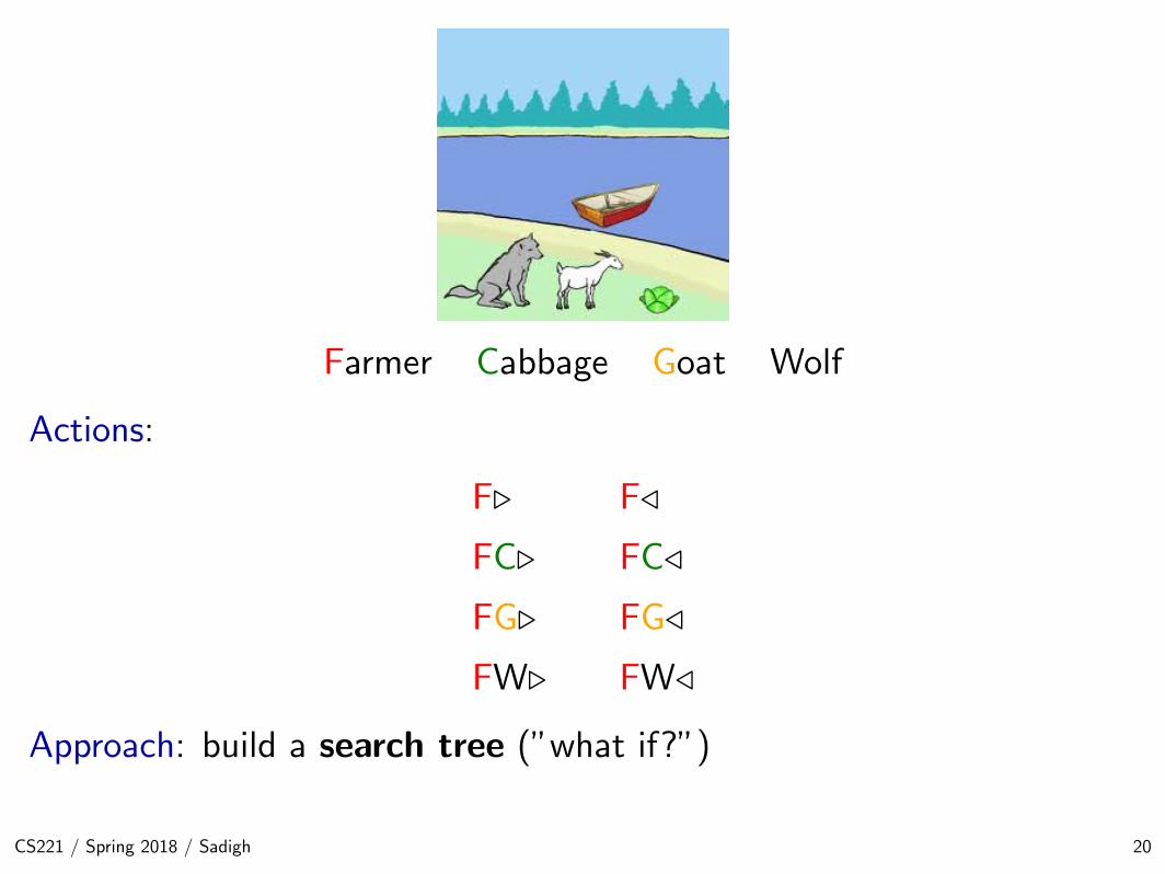
Approach: build a search tree (”what if?”)


• We first start with our boat crossing puzzle. While you can possibly solve it in more clever ways, let usapproach it in a very brain-dead, simple way, which allows us to introduce the notation for search problems.

• For this problem, we have eight possible actions, which will be denoted by a concise set of symbols. Forexample, the action FG. means that the farmer will take the goat across to the right bank; F/ means thatthe farmer is coming back to the left bank alone.

FCGW‖

GW‖FC CW‖FG

FCW‖G

W‖FCG

FW‖CG FGW‖C

G‖FCW

FG‖CW

‖FCGW

FG.:1

F/:1

FW.:1

F/:1 FG/:1

C‖FGW

FC‖GW FCG‖W

G‖FCW

FG‖CW

‖FCGW

FG.:1

F/:1

FC.:1

F/:1 FG/:1

FC.:1 FW.:1

F/:1

CG‖FW

FC.:1 FG.:1 FW.:1


Search problem

FCGW‖

GW‖FC CW‖FG

FCW‖G

W‖FCG

FW‖CG FGW‖C

G‖FCW

FG‖CW

‖FCGW

FG.:1

F/:1

FW.:1

F/:1 FG/:1

C‖FGW

FC‖GW FCG‖W

G‖FCW

FG‖CW

‖FCGW

FG.:1

F/:1

FC.:1

F/:1 FG/:1

FC.:1 FW.:1

F/:1

CG‖FW

FC.:1 FG.:1 FW.:1

Definition: search problem

• sstart: starting state

• Actions(s): possible actions

• Cost(s, a): action cost

• Succ(s, a): successor

• IsEnd(s): reached end state?


• We will build what we will call a search tree. The root of the tree is the start state sstart, and theleaves are the end states (IsEnd(s) is true). Each edge leaving a node s corresponds to a possible actiona ∈ Actions(s) that could be performed in state s. The edge is labeled with the action and its cost, writtena : Cost(s, a). The action leads deterministically to the successor state Succ(s, a), represented by the childnode.• In summary, each root-to-leaf path represents a possible action sequence, and the sum of the costs of the

edges is the cost of that path. The goal is to find the root-to-leaf path that ends in a valid end state withminimum cost.• Note that in code, we usually do not build the search tree as a concrete data structure. The search tree

is used merely to visualize the computation of the search algorithms and study the structure of the searchproblem.• For the boat crossing example, we have assumed each action (a safe river crossing) costs 1 unit of time.

We disallow actions that return us to an earlier configuration. The green nodes are the end states. The rednodes are not end states but have no successors (they result in the demise of some animal or vegetable).From this search tree, we see that there are exactly two solutions, each of which has a total cost of 7 steps.

Transportation example

Example: transportation

Street with blocks numbered 1 to n.

Walking from s to s+ 1 takes 1 minute.

Taking a magic tram from s to 2s takes 2 minutes.

How to travel from 1 to n in the least time?

[semi-live solution: TransportationProblem]


• Let’s consider another problem and practice modeling it as a search problem. Recall that this meansspecifying precisely what the states, actions, goals, costs, and successors are.

• To avoid the ambiguity of natural language, we will do this directly in code, where we define aSearchProblem class and implement the methods: startState, isEnd and succAndCost.

Backtracking search

[whiteboard: search tree]

If b actions per state, maximum depth is D actions:

• Memory: O(D) (small)

• Time: O(bD) (huge) [250 = 1125899906842624]


• Now let’s put modeling aside and suppose we are handed a search problem. How do we construct analgorithm for finding a minimum cost path (not necessarily unique)?

• We will start with backtracking search, the simplest algorithm which just tries all paths. The algorithmis called recursively on the current state s and the path leading up to that state. If we have reached a goal,then we can update the minimum cost path with the current path. Otherwise, we consider all possibleactions a from state s, and recursively search each of the possibilities.

• Graphically, backtracking search performs a depth-first traversal of the search tree. What is the time andmemory complexity of this algorithm?

• To get a simple characterization, assume that the search tree has maximum depth D (each path consistsof D actions/edges) and that there are b available actions per state (the branching factor is b).

• It is easy to see that backtracking search only requires O(D) memory (to maintain the stack for therecurrence), which is as good as it gets.

• However, the running time is proportional to the number of nodes in the tree, since the algorithm needs

to check each of them. The number of nodes is 1 + b + b2 + · · · + bD = bD+1−1b−1 = O(bD). Note that

the total number of nodes in the search tree is on the same order as the number of leaves, so the cost isalways dominated by the last level.

• In general, there might not be a finite upper bound on the depth of a search tree. In this case, there aretwo options: (i) we can simply cap the maximum depth and give up after a certain point or (ii) we candisallow visits to the same state.

• It is worth mentioning that the greedy algorithm that repeatedly chooses the lowest action myopicallywon’t work. Can you come up with an example?

Backtracking search

Algorithm: backtracking search

def backtrackingSearch(s, path):

If IsEnd(s): update minimum cost path

For each action a ∈ Actions(s):

Extend path with Succ(s, a) and Cost(s, a)

Call backtrackingSearch(Succ(s, a), path)

Return minimum cost path

[semi-live solution: backtrackingSearch]


Depth-first search

Assumption: zero action costs

Assume action costs Cost(s, a) = 0.

Idea: Backtracking search + stop when find the first end state.

If b actions per state, maximum depth is D actions:

• Space: still O(D)

• Time: still O(bD) worst case, but could be much better if solutionsare easy to find


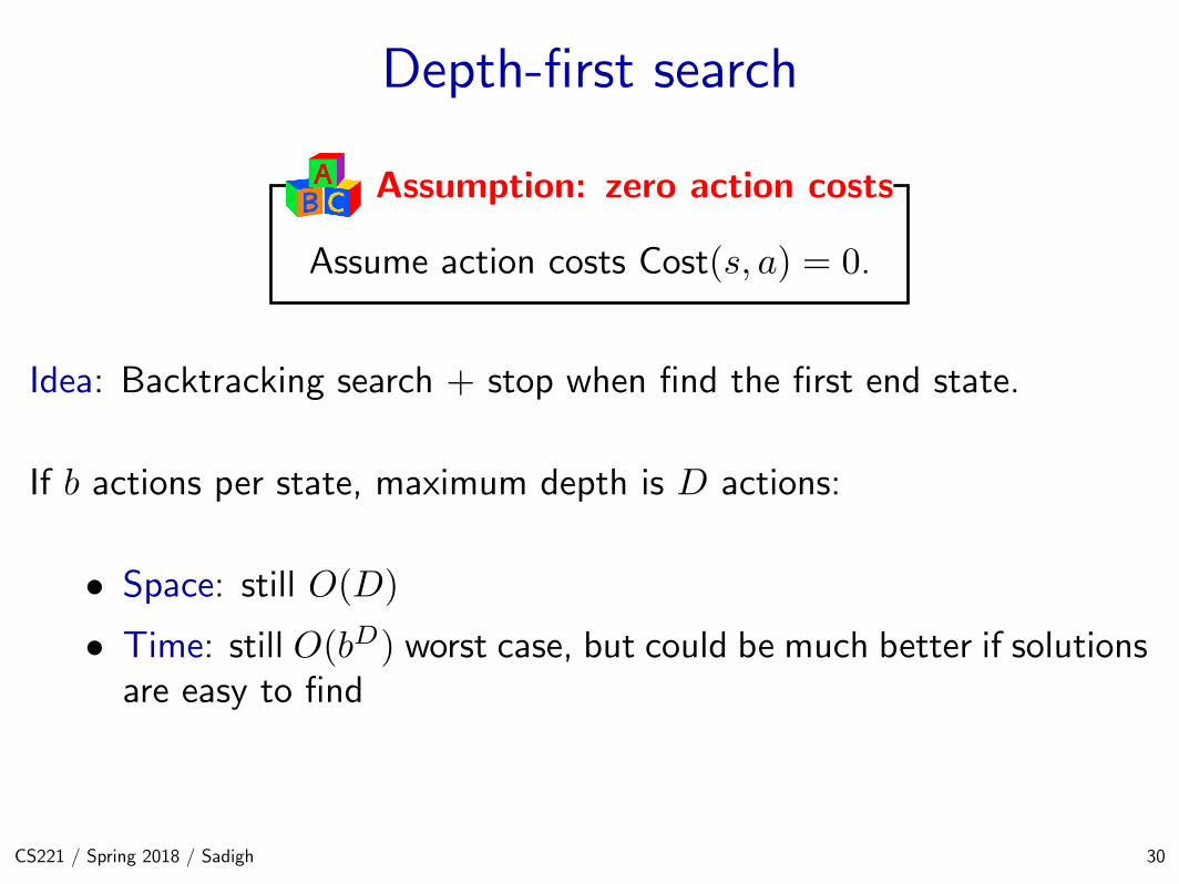
• Backtracking search will always work (i.e., find a minimum cost path), but there are cases where we cando it faster. But in order to do that, we need some additional assumptions — there is no free lunch.

• Suppose we make the assumption that all the action costs are zero. In other words, all we care about isfinding a valid action sequence that reaches the goal. Any such sequence will have the minimum cost:zero.

• In this case, we can just modify backtracking search to not keep track of costs and then stop searching assoon as we reach a goal. The resulting algorithm is depth-first search (DFS), which should be familiarto you. The worst time and space complexity are of the same order as backtracking search. In particular,if there is no path to an end state, then we have to search the entire tree.

• However, if there are many ways to reach the end state, then we can stop much earlier without exhaustingthe search tree. So DFS is great when there are an abundance of solutions.

Breadth-first search

Assumption: constant action costs

Assume action costs Cost(s, a) = c for some c ≥ 0.

Idea: explore all nodes in order of increasing depth.

Legend: b actions per state, solution has d actions

• Space: now O(bd) (a lot worse!)

• Time: O(bd) (better, depends on d, not D)


• Breadth-first search (BFS), which should also be familiar, makes a less stringent assumption, that allthe action costs are the same non-negative number. This effectively means that all the paths of a givenlength have the same cost.

• BFS maintains a queue of states to be explored. It pops a state off the queue, then pushes its successorsback on the queue.

• BFS will search all the paths consisting of one edge, two edges, three edges, etc., until it finds a paththat reaches a end state. So if the solution has d actions, then we only need to explore O(bd) nodes, thustaking that much time.

• However, a potential show-stopper is that BFS also requires O(bd) space since the queue must contain allthe nodes of a given level of the search tree. Can we do better?

DFS with iterative deepening

Assumption: constant action costs

Assume action costs Cost(s, a) = c for some c ≥ 0.

Idea:

• Modify DFS to stop at a maximum depth.

• Call DFS for maximum depths 1, 2, . . . .

DFS on d asks: is there a solution with d actions?

Legend: b actions per state, solution size d

• Space: O(d) (saved!)

• Time: O(bd) (same as BFS)


• Yes, we can do better with a trick called iterative deepening. The idea is to modify DFS to make it stopafter reaching a certain depth. Therefore, we can invoke this modified DFS to find whether a valid pathexists with at most d edges, which as discussed earlier takes O(d) space and O(bd) time.

• Now the trick is simply to invoke this modified DFS with cutoff depths of 1, 2, 3, . . . until we find asolution or give up. This algorithm is called DFS with iterative deepening (DFS-ID). In this manner, weare guaranteed optimality when all action costs are equal (like BFS), but we enjoy the parsimonious spacerequirements of DFS.

• One might worry that we are doing a lot of work, searching some nodes many times. However, keep inmind that both the number of leaves and the number of nodes in a search tree is O(bd) so asymptoticallyDFS with iterative deepening is the same time complexity as BFS.

Tree search algorithms

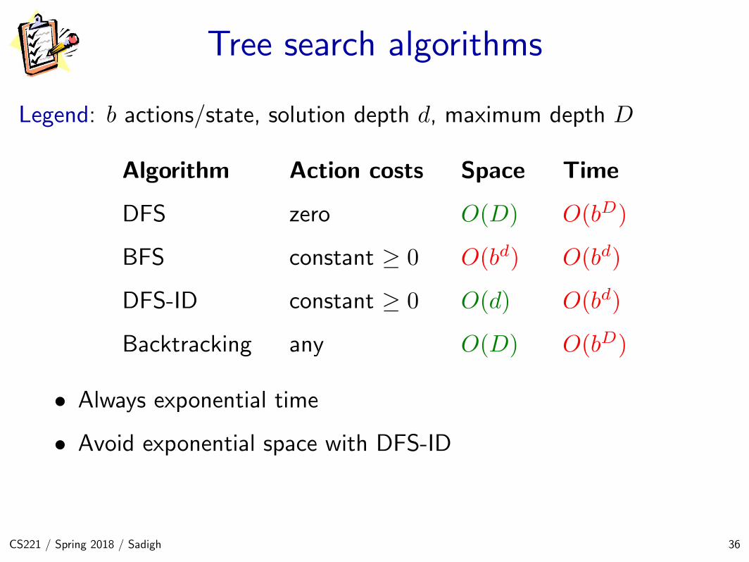
Legend: b actions/state, solution depth d, maximum depth D

Algorithm Action costs Space Time

DFS zero O(D) O(bD)

BFS constant ≥ 0 O(bd) O(bd)

DFS-ID constant ≥ 0 O(d) O(bd)

Backtracking any O(D) O(bD)

• Always exponential time

• Avoid exponential space with DFS-ID


• Here is a summary of all the tree search algorithms, the assumptions on the action costs, and the spaceand time complexities.

• The take-away is that we can’t avoid the exponential time complexity, but we can certainly have linearspace complexity. Space is in some sense the more critical dimension in search problems. Memory cannotmagically grow, whereas time ”grows” just by running an algorithm for a longer period of time, or even byparallelizing it across multiple machines (e.g., where each processor gets its own subtree to search).

Roadmap

Tree search

Dynamic programming

Uniform cost search


Dynamic programming

state s

state s′

end state

FutureCost(s′)

Cost(s, a)

Minimum cost path from state s to a end state:

FutureCost(s) =

{0 if IsEnd(s)

mina∈Actions(s)[Cost(s, a) + FutureCost(Succ(s, a))] otherwise


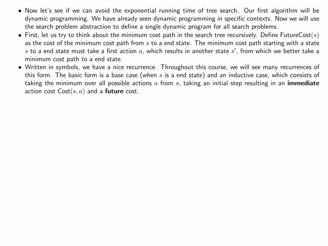
• Now let’s see if we can avoid the exponential running time of tree search. Our first algorithm will bedynamic programming. We have already seen dynamic programming in specific contexts. Now we will usethe search problem abstraction to define a single dynamic program for all search problems.

• First, let us try to think about the minimum cost path in the search tree recursively. Define FutureCost(s)as the cost of the minimum cost path from s to a end state. The minimum cost path starting with a states to a end state must take a first action a, which results in another state s′, from which we better take aminimum cost path to a end state.

• Written in symbols, we have a nice recurrence. Throughout this course, we will see many recurrences ofthis form. The basic form is a base case (when s is a end state) and an inductive case, which consists oftaking the minimum over all possible actions a from s, taking an initial step resulting in an immediateaction cost Cost(s, a) and a future cost.

Motivating task

Example: route finding

Find the minimum cost path from city 1 to city n, only movingforward. It costs cij to go from i to j.

1

2

3

4

5

6

7

7

6

7

7

5

6

7

7

6

7

7

4

5

6

7

7

6

7

7

5

6

7

7

6

7

7

3

4

5

6

7

7

6

7

7

5

6

7

7

6

7

7

4

5

6

7

7

6

7

7

5

6

7

7

6

7

7

Observation: future costs only depend on current city


• Now let us see if we can avoid the exponential time. If we consider the simple route finding problem oftraveling from city 1 to city n, the search tree grows exponentially with n.

• However, upon closer inspection, we note that this search tree has a lot of repeated structures. Moreover(and this is important), the future costs (the minimum cost of reaching a end state) of a state only dependson the current city! So therefore, all the subtrees rooted at city 5, for example, have the same minimumcost!

• If we can just do that computation once, then we will have saved big time. This is the central idea ofdynamic programming.

• We’ve already reviewed dynamic programming in the first lecture. The purpose here is to construct onegeneric dynamic programming solution that will work on any search problem. Again, this highlights theuseful division between modeling (defining the search problem) and algorithms (performing the actualsearch).

Dynamic programming

State: past sequence of actions current city

1

2

34

5

6

7

Exponential saving in time and space!


• Let us collapse all the nodes that have the same city into one. This provides us with no longer a tree, buta directed acyclic graph with only n nodes rather than exponential in n nodes.

• Note that dynamic programming is only useful if we can define a search problem where the number ofstates is small enough to fit in memory.

Dynamic programming

Algorithm: dynamic programming

def DynamicProgramming(s):

If already computed for s, return cached answer.

If IsEnd(s): return solution

For each action a ∈ Actions(s): ...

[semi-live solution: Dynamic Programming]

Assumption: acyclicity

The state graph defined by Actions(s) and Succ(s, a) is acyclic.


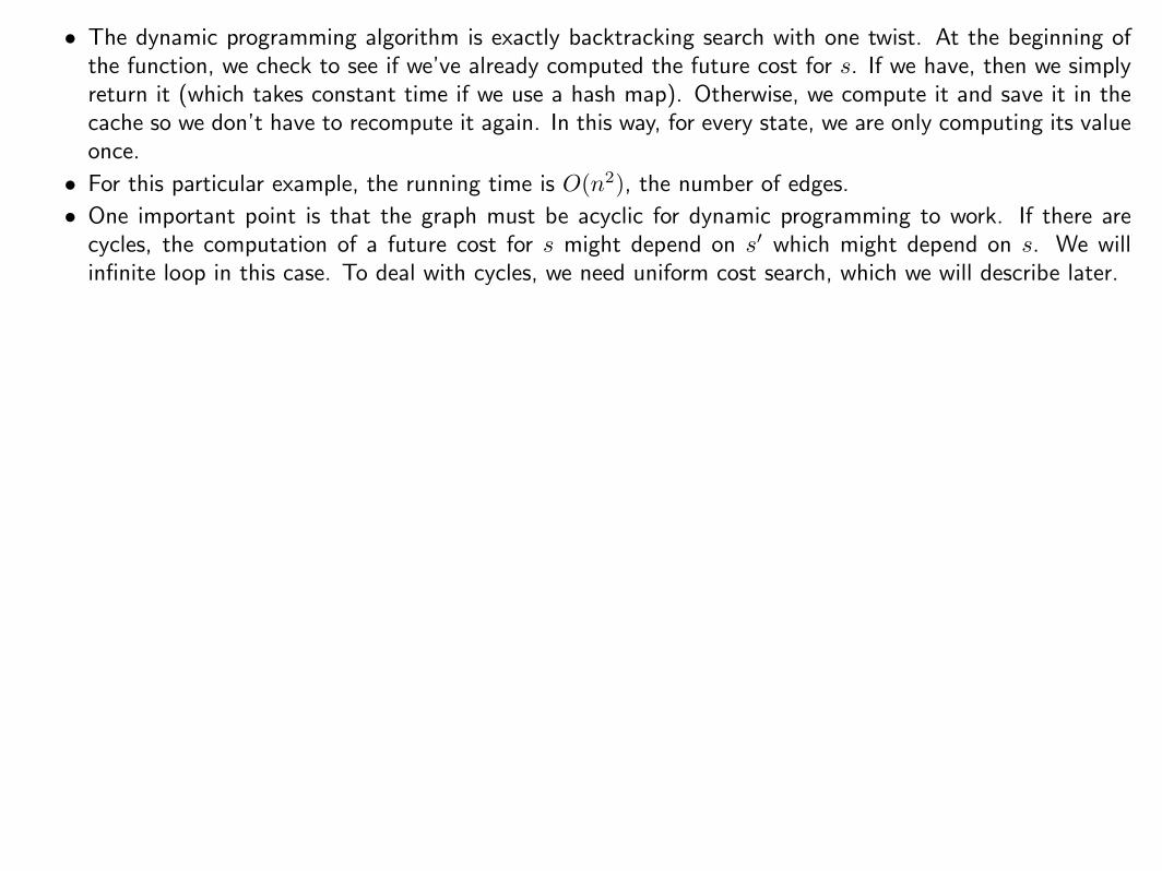
• The dynamic programming algorithm is exactly backtracking search with one twist. At the beginning ofthe function, we check to see if we’ve already computed the future cost for s. If we have, then we simplyreturn it (which takes constant time if we use a hash map). Otherwise, we compute it and save it in thecache so we don’t have to recompute it again. In this way, for every state, we are only computing its valueonce.

• For this particular example, the running time is O(n2), the number of edges.

• One important point is that the graph must be acyclic for dynamic programming to work. If there arecycles, the computation of a future cost for s might depend on s′ which might depend on s. We willinfinite loop in this case. To deal with cycles, we need uniform cost search, which we will describe later.

Dynamic programming

Key idea: state

A state is a summary of all the past actions sufficient to choosefuture actions optimally.

past actions (all cities) 1 3 4 6

state (current city) 1 3 4 6


• So far, we have only considered the example where the cost only depends on the current city. But let’s tryto capture exactly what’s going on more generally.

• This is perhaps the most important idea of this lecture: state. A state is a summary of all the past actionssufficient to choose future actions optimally.

• What state is really about is forgetting the past. We can’t forget everything because the action costs inthe future might depend on what we did on the past. The more we forget, the fewer states we have, andthe more efficient our algorithm. So the name of the game is to find the minimal set of states that suffice.It’s a fun game.

Handling additional constraints

Example: route finding

Find the minimum cost path from city 1 to city n, only movingforward. It costs cij to go from i to j.

Constraint: Can’t visit three odd cities in a row.

State: (whether previous city was odd, current city)

n/a, 1

odd, 3

odd, 7 odd, 4

7:c37 4:c34

odd, 4

even, 5

5:c45

3:c13 4:c14


• Let’s add a constraint that says we can’t visit three odd cities in a row. If we only keep track of the currentcity, and we try to move to a next city, we cannot enforce this constraint because we don’t know what theprevious city was. So let’s add the previous city into the state.

• This will work, but we can actually make the state smaller. We only need to keep track of whether theprevious city was an odd numbered city to enforce this constraint.

• Note that in doing so, we have 2n states rather than n2 states, which is a substantial savings. So thelesson is to pay attention to what information you actually need in the state.

Question

Objective: travel from city 1 to city n, visiting at least 3 odd cities.What is the minimal state?



State graph

State: (min(number of odd cities visited, 3), current city)

1,1

1,2

1,3 1,4

1,5

1,6

2,1

2,2

2,3 2,4

2,5

2,6

3,1

3,2

3,3 3,4

3,5

3,6


• Our first thought might be to remember how many odd cities we have visited so far (and the current city).

• But if we’re more clever, we can notice that once the number of odd cities is 3, we don’t need tokeep track of whether that number goes up to 4 or 5, etc. So the state we actually need to keep is(min(number of odd cities visited, 3), current city). Thus, our state space is O(n) rather than O(n2).

• We can visualize what augmenting the state does to the state graph. Effectively, we are copying each node4 times, and the edges are redirected to move between these copies.

• Note that some states such as (2, 1) aren’t reachable (if you’re in city 1, it’s impossible to have visited 2odd cities already); the algorithm will not touch those states and that’s perfectly okay.

Question

Objective: travel from city 1 to city n, visiting more odd than even cities.What is the minimal state?



• An initial guess might be to keep track of the number of even cities and the number of odd cities visited.

• But we can do better. We have to just keep track of the number of odd cities minus the number of evencities and the current city. We can write this more formally as (n1 − n2, current city), where n1 is thenumber of odd cities visited so far and n2 is the number of even cities visited so far.

Summary

• State: summary of past actions sufficient to choose future actionsoptimally

• Dynamic programming: backtracking search with memoization— potentially exponential savings

Dynamic programming only works for acyclic graphs...what if there arecycles?


Roadmap

Tree search

Dynamic programming

Uniform cost search


Ordering the states

Observation: prefixes of optimal path are optimal

sstart s s′

PastCost(s) Cost(s, a)

Key: if graph is acyclic, dynamic programming makes sure we computePastCost(s) before PastCost(s′)

If graph is cyclic, then we need another mechanism to order states...


• Recall that we used dynamic programming to compute the future cost of each state s, the cost of theminimum cost path from s to a end state.

• We can analogously define PastCost(s), the cost of the minimum cost path from the start state to s. Ifinstead of having access to the successors via Succ(s, a), we had access to predecessors (think of reversingthe edges in the state graph), then we could define a dynamic program to compute all the PastCost(s).

• Dynamic programming relies on the absence of cycles, so that there was always a clear order in which tocompute all the past costs. If the past costs of all the predecessors of a state s are computed, then wecould compute the past cost of s by taking the minimum.

• Note that PastCost(s) will always be computed before PastCost(s′) if there is an edge from s to s′. Inessence, the past costs will be computed according to a topological ordering of the nodes.

• However, when there are cycles, no topological ordering exists, so we need another way to order the states.

Uniform cost search (UCS)

Key idea: state ordering

UCS enumerates states in order of increasing past cost.

Assumption: non-negativity

All action costs are non-negative: Cost(s, a) ≥ 0.

UCS in action:


• The key idea that uniform cost search (UCS) uses is to compute the past costs in order of increasingpast cost. To make this efficient, we need to make an important assumption that all action costs arenon-negative.

• This assumption is reasonable in many cases, but doesn’t allow us to handle cases where actions havepayoff. To handle negative costs (positive payoffs), we need the Bellman-Ford algorithm. When we talkabout value iteration for MDPs, we will see a form of this algorithm.

• Note: those of you who have studied algorithms should immediately recognize UCS as Dijkstra’s algorithm.Logically, the two are indeed equivalent. There is an important implementation difference: UCS takes asinput a search problem, which implicitly defines a large and even infinite graph, whereas Dijkstra’salgorithm (in the typical exposition) takes as input a fully concrete graph. The implicitness is importantin practice because we might be working with an enormous graph (a detailed map of world) but only needto find the path between two close by points (Stanford to Palo Alto).

• Another difference is that Dijkstra’s algorithm is usually thought of as finding the shortest path from thestart state to every other node, whereas UCS is explicitly about finding the shortest path to an end state.This difference is sharpened when we look at the A* algorithm next time, where knowing that we’re tryingto get to the goal can yield a much faster algorithm. The name uniform cost search refers to the fact thatwe are exploring states of the same past cost uniformly (the video makes this visually clear); in contrast,A* will explore states which are biased towards the end state.

High-level strategy

Frontier

Explored

Unexplored

• Explored: states we’ve found the optimal path to

• Frontier: states we’ve seen, still figuring out how to get therecheaply

• Unexplored: states we haven’t seen


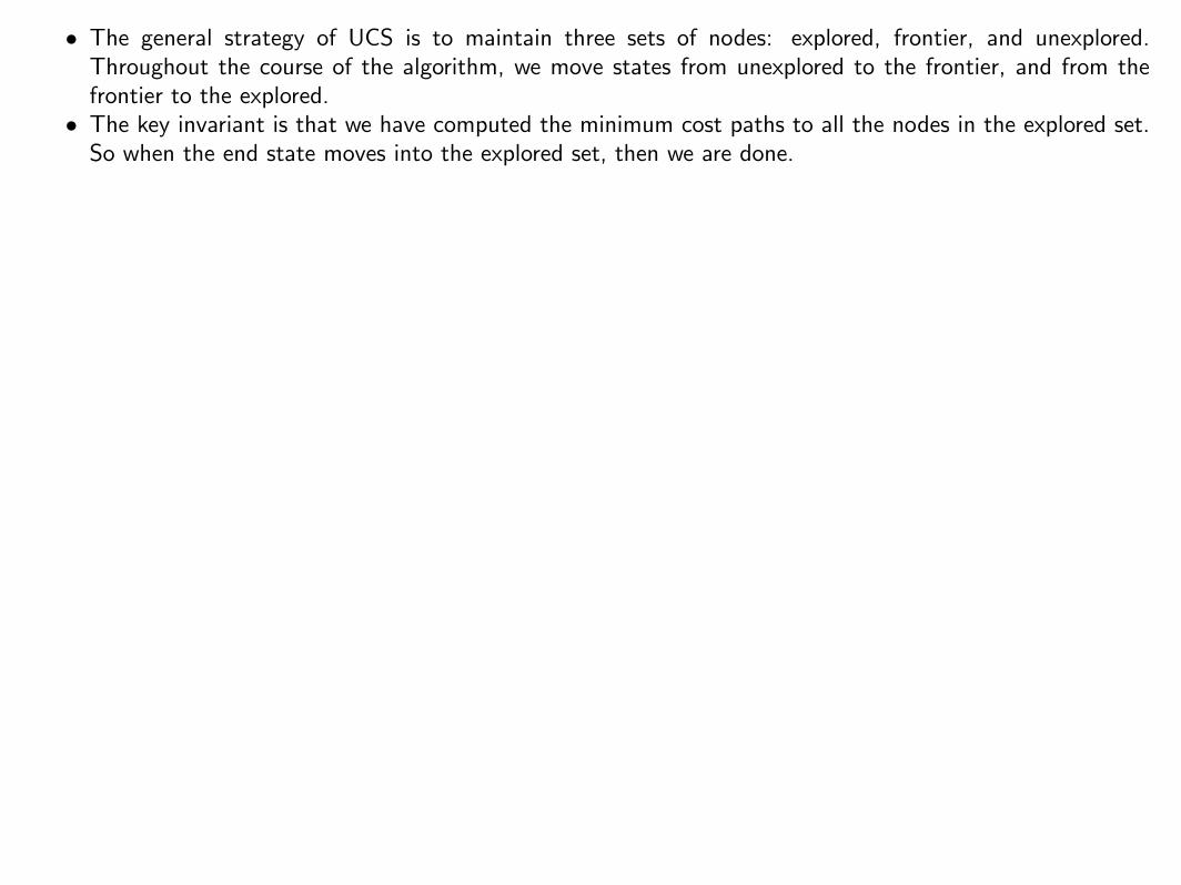
• The general strategy of UCS is to maintain three sets of nodes: explored, frontier, and unexplored.Throughout the course of the algorithm, we move states from unexplored to the frontier, and from thefrontier to the explored.

• The key invariant is that we have computed the minimum cost paths to all the nodes in the explored set.So when the end state moves into the explored set, then we are done.

Uniform cost search example

Example: UCS example

A

B

C

D

Start state: A, end state: D

[whiteboard]

Minimum cost path:

A → B → C → D with cost 3


• Before we present the full algorithm, let’s walk through a concrete example.

• Initially, we put A on the frontier. We then take A off the frontier and mark it as explored. We add B andC to the frontier with past costs 1 and 100, respectively.

• Next, we remove from the frontier the state with the minimum past cost (priority), which is B. We markB as explored and consider successors A, C, D. We ignore A since it’s already explored. The past cost ofC gets updated from 100 to 2. We add D to the frontier with initial past cost 101.

• Next, we remove C from the frontier; its successors are A, B, D. A and B are already explored, so we onlyupdate D’s past cost from 101 to 3.

• Finally, we pop D off the frontier, find that it’s a end state, and terminate the search.

Uniform cost search (UCS)

Algorithm: uniform cost search [Dijkstra, 1956]

Add sstart to frontier (priority queue)

Repeat until frontier is empty:

Remove s with smallest priority p from frontier

If IsEnd(s): return solution

Add s to explored

For each action a ∈ Actions(s):

Get successor s′ ← Succ(s, a)

If s′ already in explored: continue

Update frontier with s′ and priority p+ Cost(s, a)

[semi-live solution: Uniform Cost Search]


• Implementation note: we use util.PriorityQueue which supports removeMin and update. Note thatfrontier.update(state, pastCost) returns whether pastCost improves the existing estimate of thepast cost of state.

Analysis of uniform cost search

Theorem: correctness

When a state s is popped from the frontier and moved to explored,its priority is PastCost(s), the minimum cost to s.

Proof:

Explored

sstart s

t u


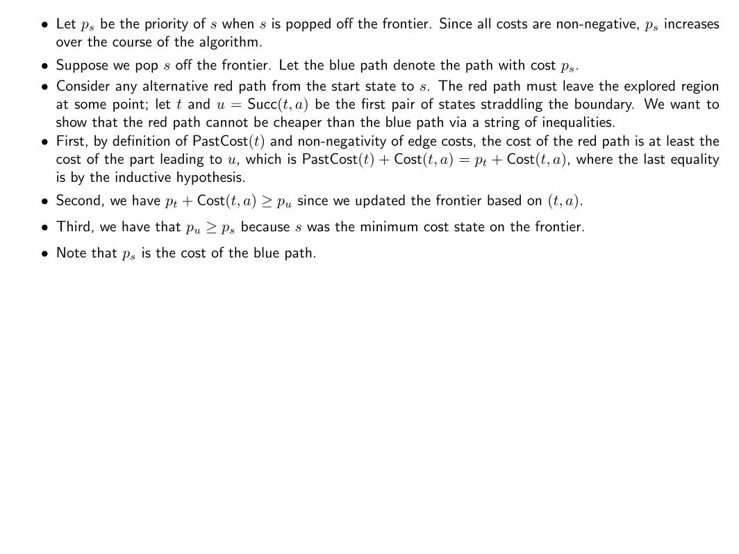
• Let ps be the priority of s when s is popped off the frontier. Since all costs are non-negative, ps increasesover the course of the algorithm.

• Suppose we pop s off the frontier. Let the blue path denote the path with cost ps.

• Consider any alternative red path from the start state to s. The red path must leave the explored regionat some point; let t and u = Succ(t, a) be the first pair of states straddling the boundary. We want toshow that the red path cannot be cheaper than the blue path via a string of inequalities.

• First, by definition of PastCost(t) and non-negativity of edge costs, the cost of the red path is at least thecost of the part leading to u, which is PastCost(t) + Cost(t, a) = pt + Cost(t, a), where the last equalityis by the inductive hypothesis.

• Second, we have pt + Cost(t, a) ≥ pu since we updated the frontier based on (t, a).

• Third, we have that pu ≥ ps because s was the minimum cost state on the frontier.

• Note that ps is the cost of the blue path.

DP versus UCS

N total states, n of which are closer than end state

Algorithm Cycles? Action costs Time/space

DP no any O(N)

UCS yes ≥ 0 O(n log n)

Note: UCS potentially explores fewer states, but requires more overheadto maintain the priority queue

Note: assume number of actions per state is constant (independent ofn and N)


• DP and UCS have complementary strengths and weaknesses; neither dominates the other.

• DP can handle negative action costs, but is restricted to acyclic graphs. It also explores all N reachablestates from sstart, which is inefficient. This is unavoidable due to negative action costs.

• UCS can handle cyclic graphs, but is restricted to non-negative action costs. An advantage is that it onlyneeds to explore n states, where n is the number of states which are cheaper to get to than any end state.However, there is an overhead with maintaining the priority queue.

• One might find it unsatisfying that UCS can only deal with non-negative action costs. Can we just add alarge positive constant to each action cost to make them all non-negative? It turns out this doesn’t workbecause it penalizes longer paths more than shorter paths, so we would end up solving a different problem.

Summary

• Tree search: memory efficient, suitable for huge state spaces butexponential worst-case running time

• State: summary of past actions sufficient to choose future actionsoptimally

• Graph search: dynamic programming and uniform cost search con-struct optimal paths (exponential savings!)

• Next time: learning action costs, searching faster with A*


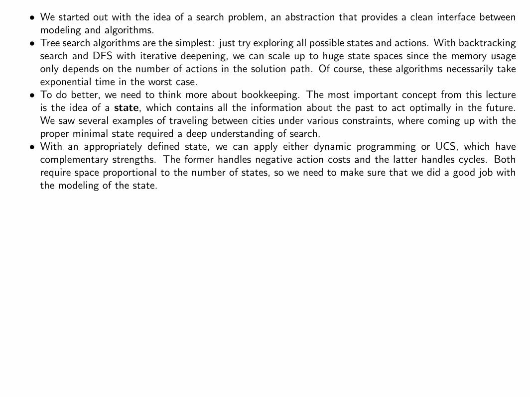
• We started out with the idea of a search problem, an abstraction that provides a clean interface betweenmodeling and algorithms.

• Tree search algorithms are the simplest: just try exploring all possible states and actions. With backtrackingsearch and DFS with iterative deepening, we can scale up to huge state spaces since the memory usageonly depends on the number of actions in the solution path. Of course, these algorithms necessarily takeexponential time in the worst case.

• To do better, we need to think more about bookkeeping. The most important concept from this lectureis the idea of a state, which contains all the information about the past to act optimally in the future.We saw several examples of traveling between cities under various constraints, where coming up with theproper minimal state required a deep understanding of search.

• With an appropriately defined state, we can apply either dynamic programming or UCS, which havecomplementary strengths. The former handles negative action costs and the latter handles cycles. Bothrequire space proportional to the number of states, so we need to make sure that we did a good job withthe modeling of the state.

Documents

Lecture 5: Search I · · 2018-03-27A farmer wants to get his cabbage , goat , and wolf across a ... Now we will proceed to the rst type of state-based models, search problems