Lecture 5: Similarity and Clustering

(Chap 4, Charkrabarti)

Wen-Hsiang Lu (盧文祥 )Department of Computer Science and

Information Engineering,National Cheng Kung University

2004/10/21

Similarity and Clustering

Clustering 3

Motivation• Problem 1: Query word could be

ambiguous:– Eg: Query“Star” retrieves documents about

astronomy, plants, animals etc. – Solution: Visualisation

• Clustering document responses to queries along lines of different topics.

• Problem 2: Manual construction of topic hierarchies and taxonomies– Solution:

• Preliminary clustering of large samples of web documents.

• Problem 3: Speeding up similarity search– Solution:

• Restrict the search for documents similar to a query to most representative cluster(s).

Clustering 4

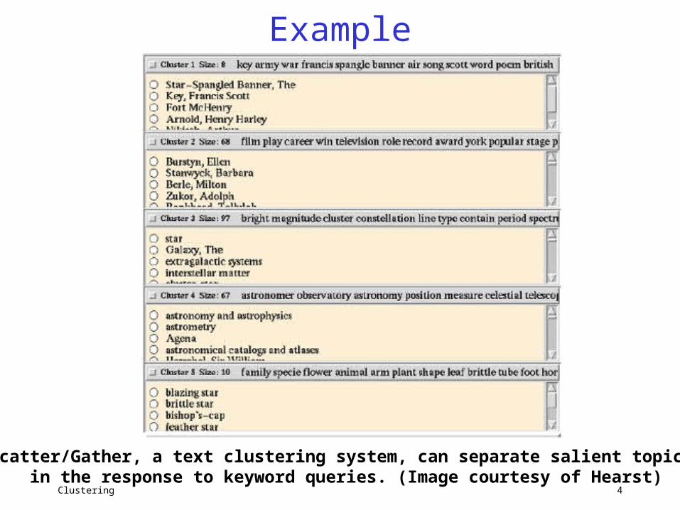
Example

Scatter/Gather, a text clustering system, can separate salient topics in the response to keyword queries. (Image courtesy of Hearst)

Clustering 5

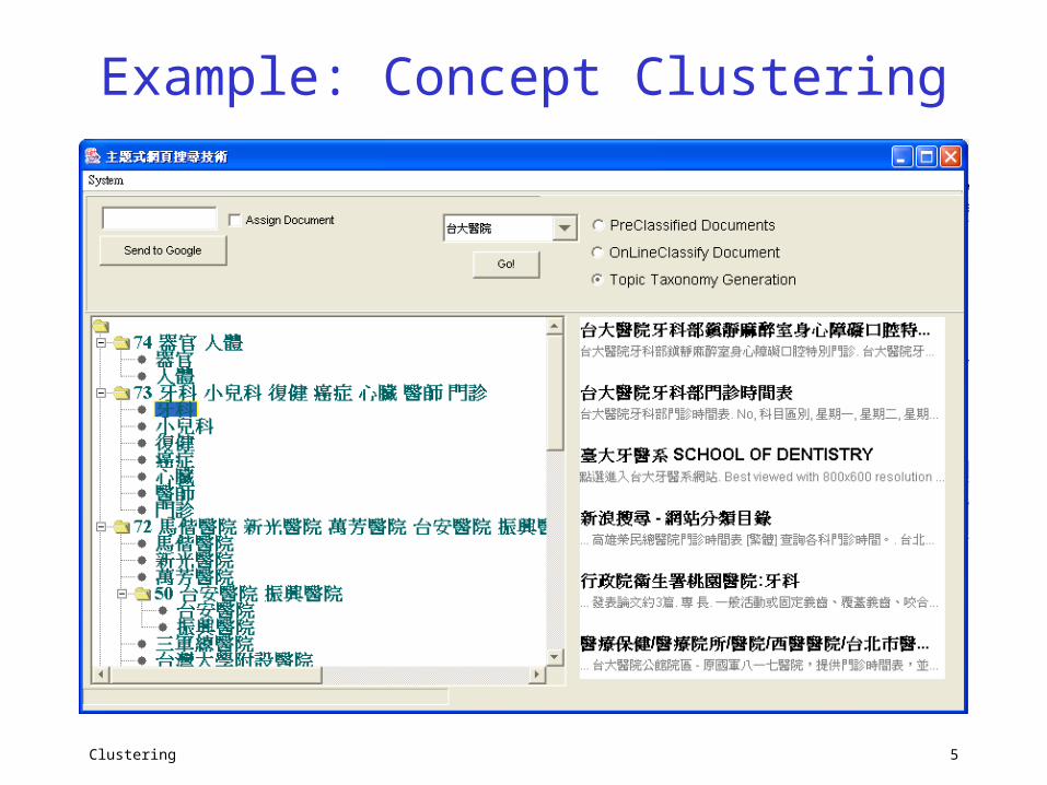
Example: Concept Clustering

Clustering 6

Clustering• Task : Evolve measures of similarity to cluster a collection of

documents/terms into groups within which similarity within a cluster is larger than across clusters.

• Cluster Hypothesis: Given a `suitable‘ clustering of a collection, if the user is interested in document/term d/t, he is likely to be interested in other members of the cluster to which d/t belongs.

• Similarity measures– Represent documents by TFIDF vectors– Distance between document vectors– Cosine of angle between document vectors

• Issues– Large number of noisy dimensions– Notion of noise is application dependent

Clustering 7

Clustering (cont…)

• Collaborative filtering: Clustering of two/more objects which have bipartite relationship

• Two important paradigms: – Bottom-up agglomerative clustering– Top-down partitioning

• Visualisation techniques: Embedding of corpus in a low-dimensional space

• Characterising the entities: – Internally : Vector space model, probabilistic models– Externally: Measure of similarity/dissimilarity

between pairs

• Learning: Supplement stock algorithms with experience with data

Clustering 8

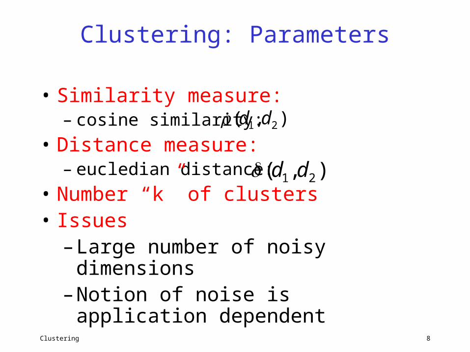
Clustering: Parameters

• Similarity measure: – cosine similarity:

• Distance measure:– eucledian distance:

• Number “k” of clusters• Issues

– Large number of noisy dimensions

– Notion of noise is application dependent

),( 21 dd

),( 21 dd

Clustering 9

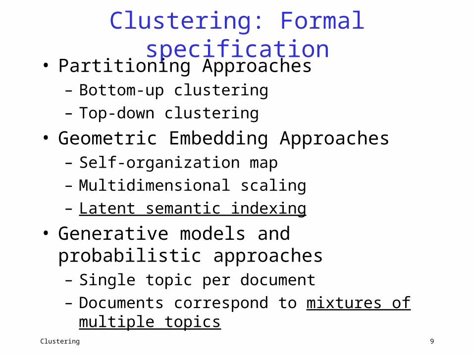
Clustering: Formal specification• Partitioning Approaches

– Bottom-up clustering– Top-down clustering

• Geometric Embedding Approaches– Self-organization map– Multidimensional scaling– Latent semantic indexing

• Generative models and probabilistic approaches– Single topic per document– Documents correspond to mixtures of

multiple topics

Clustering 10

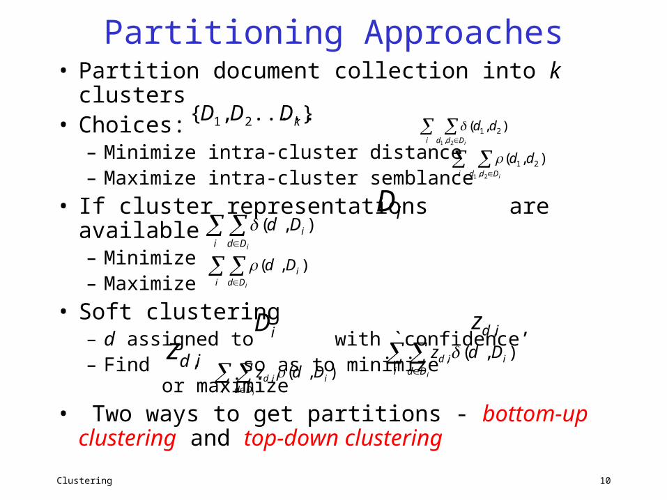
Partitioning Approaches• Partition document collection into k

clusters • Choices:

– Minimize intra-cluster distance– Maximize intra-cluster semblance

• If cluster representations are available– Minimize – Maximize

• Soft clustering– d assigned to with `confidence’ – Find so as to minimize or

maximize

• Two ways to get partitions - bottom-up clustering and top-down clustering

}.....,{ 21 kDDD

i Ddd i

dd21 ,

21 ),(

i Ddd i

dd21 ,

21 ),(

i Dd

i

i

Dd ),(

iDi Dd

i

i

Dd ),(

iD idz ,

idz , i Dd

iid

i

Ddz ),(,

i Ddiid

i

Ddz ),(,

Clustering 11

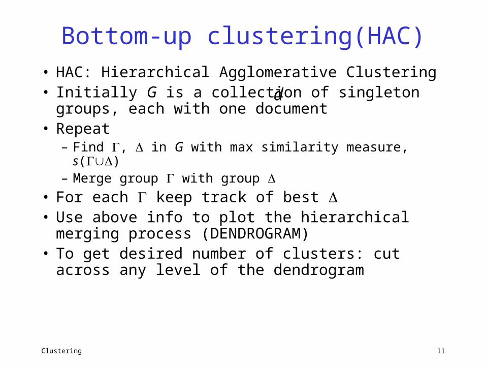
Bottom-up clustering(HAC)• HAC: Hierarchical Agglomerative Clustering• Initially G is a collection of singleton groups,

each with one document • Repeat

– Find , in G with max similarity measure, s()– Merge group with group

• For each keep track of best • Use above info to plot the hierarchical merging

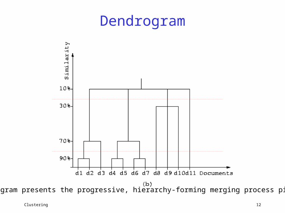
process (DENDROGRAM)• To get desired number of clusters: cut across

any level of the dendrogram

d

Clustering 12

Dendrogram

A dendogram presents the progressive, hierarchy-forming merging process pictorially.

Clustering 13

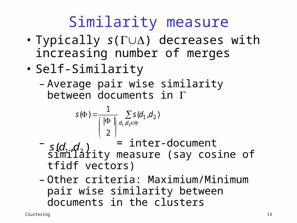
Similarity measure• Typically s() decreases with

increasing number of merges • Self-Similarity

– Average pair wise similarity between documents in

– = inter-document similarity measure (say cosine of tfidf vectors)

– Other criteria: Maximium/Minimum pair wise similarity between documents in the clusters

21 ,21 ),(

2

||

1)(

ddddss

),( 21 dds

Clustering 14

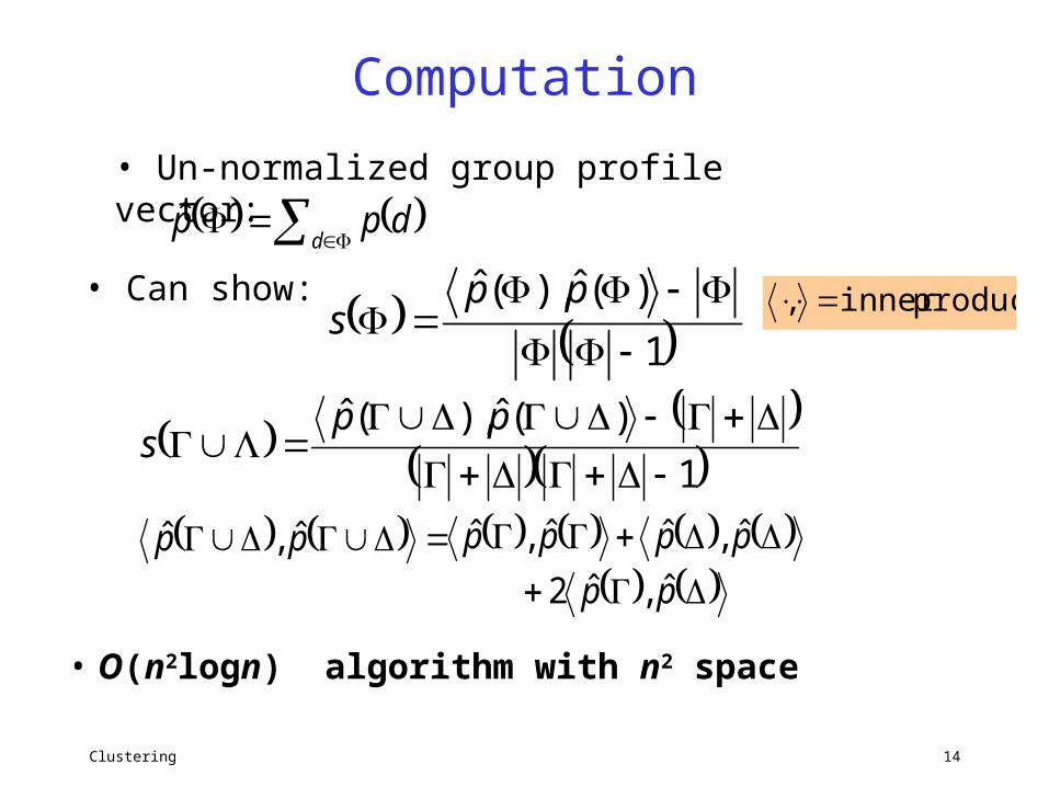
Computation

• Un-normalized group profile vector:

ddpp̂

• Can show: 1)(ˆ),(ˆ

pps

1

)(ˆ),(ˆ

pp

s

pp

pppppp

ˆ,ˆ2

ˆ,ˆˆ,ˆˆ,ˆ

• O(n2logn) algorithm with n2 space

productinner ,

Clustering 15

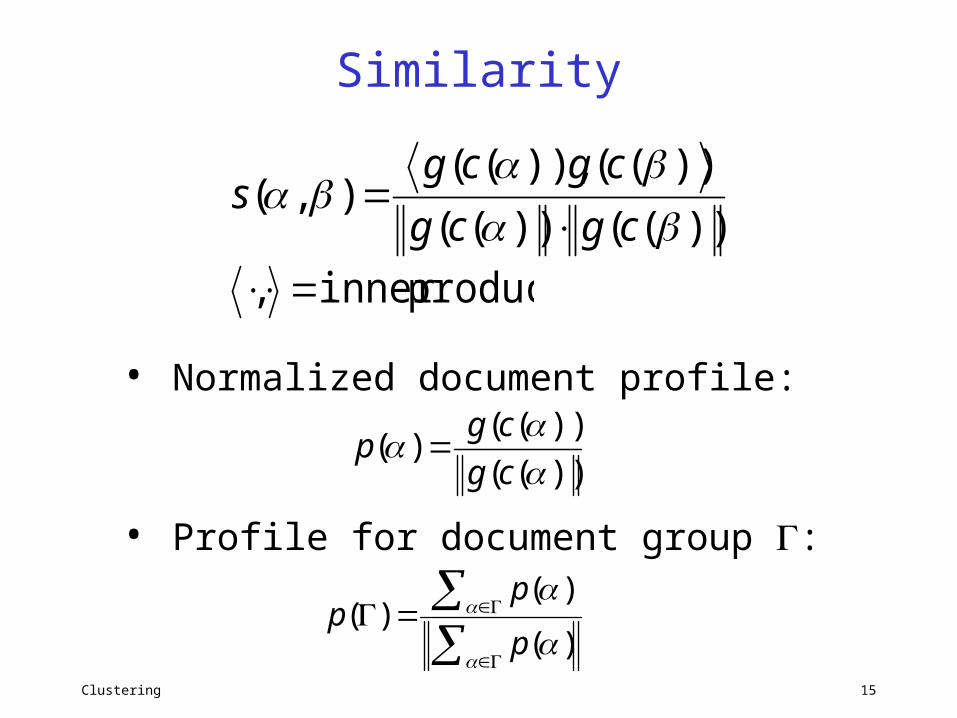
Similarity

))(())((

))(()),((),(

cgcg

cgcgs

productinner ,

• Normalized document profile:

))((

))(()(

cg

cgp

• Profile for document group :

)(

)()(

p

pp

Clustering 16

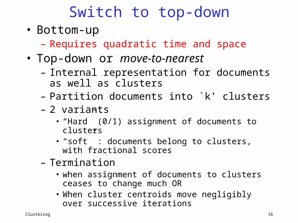
Switch to top-down• Bottom-up

– Requires quadratic time and space

• Top-down or move-to-nearest– Internal representation for documents as

well as clusters– Partition documents into `k’ clusters– 2 variants

• “Hard” (0/1) assignment of documents to clusters• “soft” : documents belong to clusters, with

fractional scores

– Termination • when assignment of documents to clusters ceases

to change much OR• When cluster centroids move negligibly over

successive iterations

Clustering 17

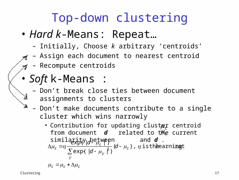
Top-down clustering• Hard k-Means: Repeat…

– Initially, Choose k arbitrary ‘centroids’– Assign each document to nearest centroid – Recompute centroids

• Soft k-Means : – Don’t break close ties between document

assignments to clusters– Don’t make documents contribute to a single cluster

which wins narrowly• Contribution for updating cluster centroid from

document d related to the current similarity between and d .

cc

ccc

cc

c dd

d

rate learning theis ),()||exp(

)||exp(2

2

Clustering 18

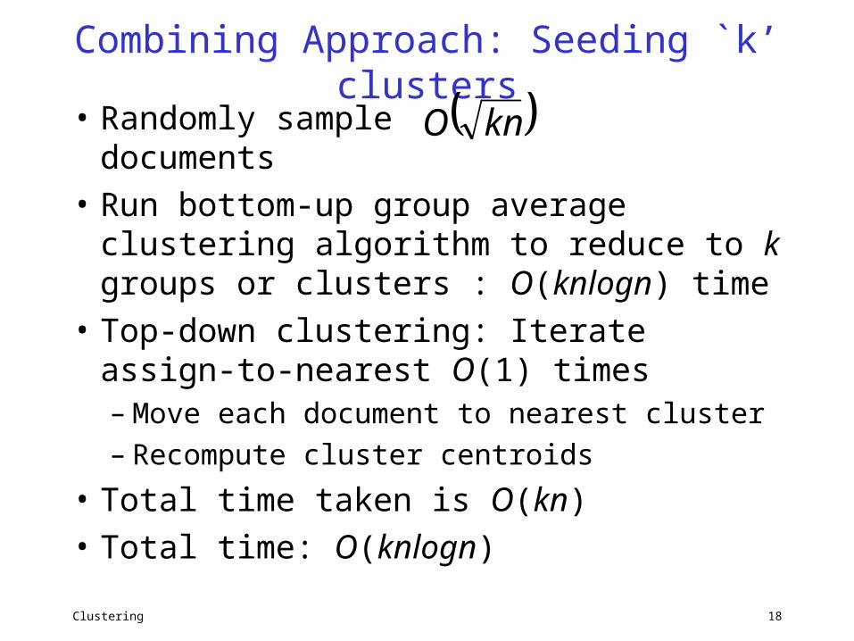
Combining Approach: Seeding `k’ clusters

• Randomly sample documents

• Run bottom-up group average clustering algorithm to reduce to k groups or clusters : O(knlogn) time

• Top-down clustering: Iterate assign-to-nearest O(1) times– Move each document to nearest cluster– Recompute cluster centroids

• Total time taken is O(kn)• Total time: O(knlogn)

knO

Clustering 19

Choosing `k’• Mostly problem driven• Could be ‘data driven’ only when

either– Data is not sparse– Measurement dimensions are not too

noisy

• Interactive– Data analyst interprets results of

structure discovery

Clustering 20

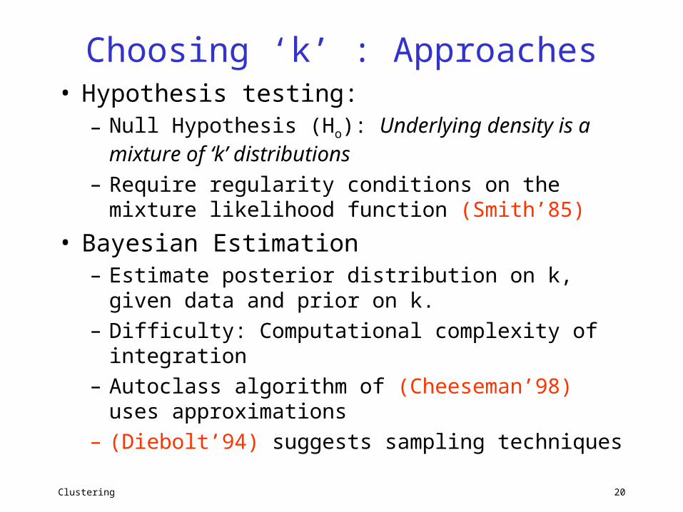
Choosing ‘k’ : Approaches• Hypothesis testing:

– Null Hypothesis (Ho): Underlying density is a mixture of ‘k’ distributions

– Require regularity conditions on the mixture likelihood function (Smith’85)

• Bayesian Estimation– Estimate posterior distribution on k, given

data and prior on k.– Difficulty: Computational complexity of

integration– Autoclass algorithm of (Cheeseman’98) uses

approximations– (Diebolt’94) suggests sampling techniques

Clustering 21

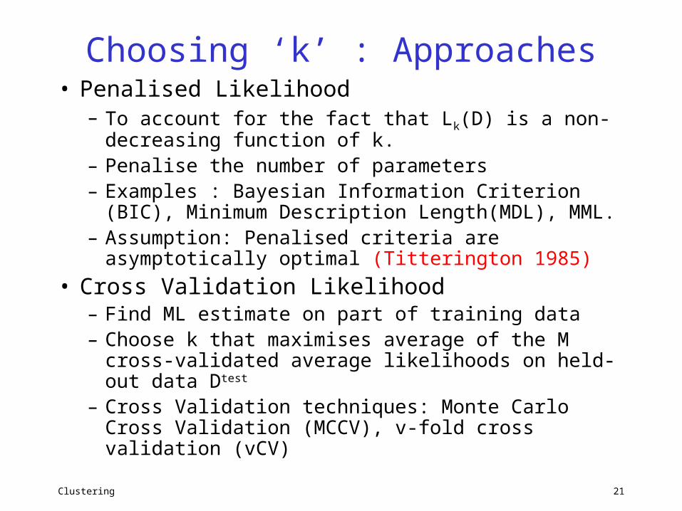
Choosing ‘k’ : Approaches• Penalised Likelihood

– To account for the fact that Lk(D) is a non-decreasing function of k.

– Penalise the number of parameters– Examples : Bayesian Information Criterion

(BIC), Minimum Description Length(MDL), MML.– Assumption: Penalised criteria are

asymptotically optimal (Titterington 1985)

• Cross Validation Likelihood– Find ML estimate on part of training data– Choose k that maximises average of the M

cross-validated average likelihoods on held-out data Dtest

– Cross Validation techniques: Monte Carlo Cross Validation (MCCV), v-fold cross validation (vCV)

Clustering 22

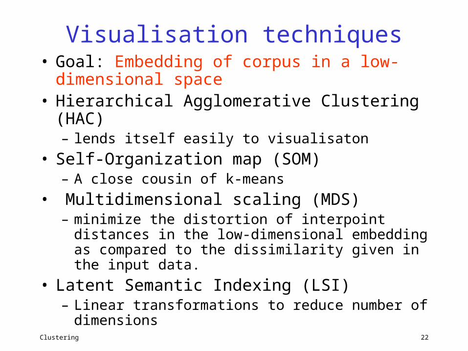
Visualisation techniques• Goal: Embedding of corpus in a low-

dimensional space• Hierarchical Agglomerative Clustering

(HAC)– lends itself easily to visualisaton

• Self-Organization map (SOM) – A close cousin of k-means

• Multidimensional scaling (MDS)– minimize the distortion of interpoint distances

in the low-dimensional embedding as compared to the dissimilarity given in the input data.

• Latent Semantic Indexing (LSI)– Linear transformations to reduce number of

dimensions

Clustering 23

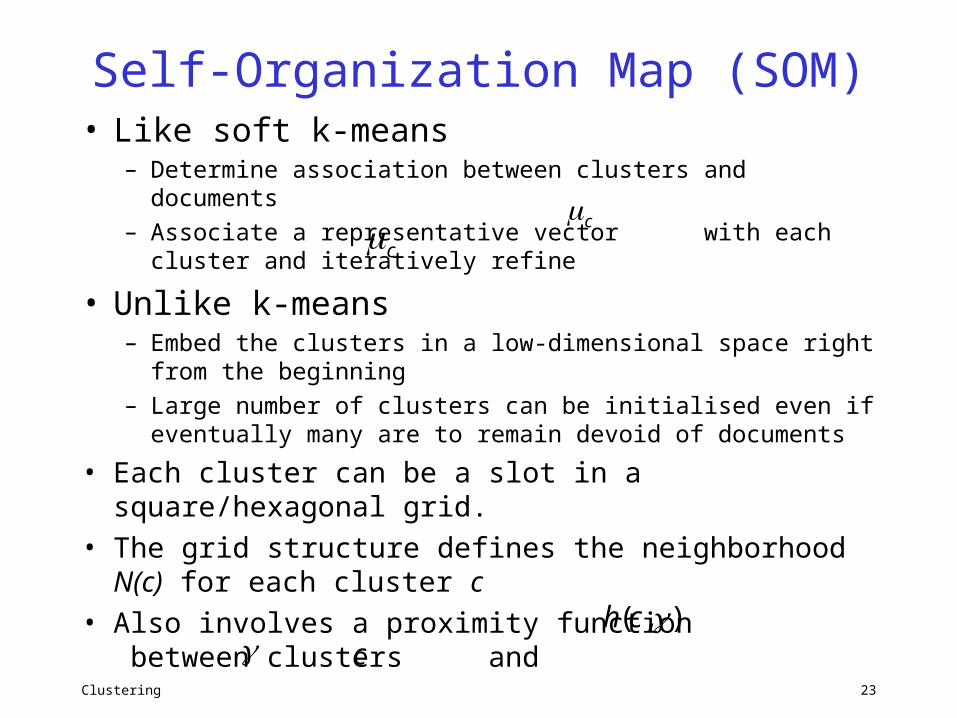
Self-Organization Map (SOM)• Like soft k-means

– Determine association between clusters and documents– Associate a representative vector with each cluster

and iteratively refine

• Unlike k-means– Embed the clusters in a low-dimensional space right

from the beginning– Large number of clusters can be initialised even if

eventually many are to remain devoid of documents

• Each cluster can be a slot in a square/hexagonal grid.

• The grid structure defines the neighborhood N(c) for each cluster c

• Also involves a proximity function between clusters and

cc

c),( ch

Clustering 24

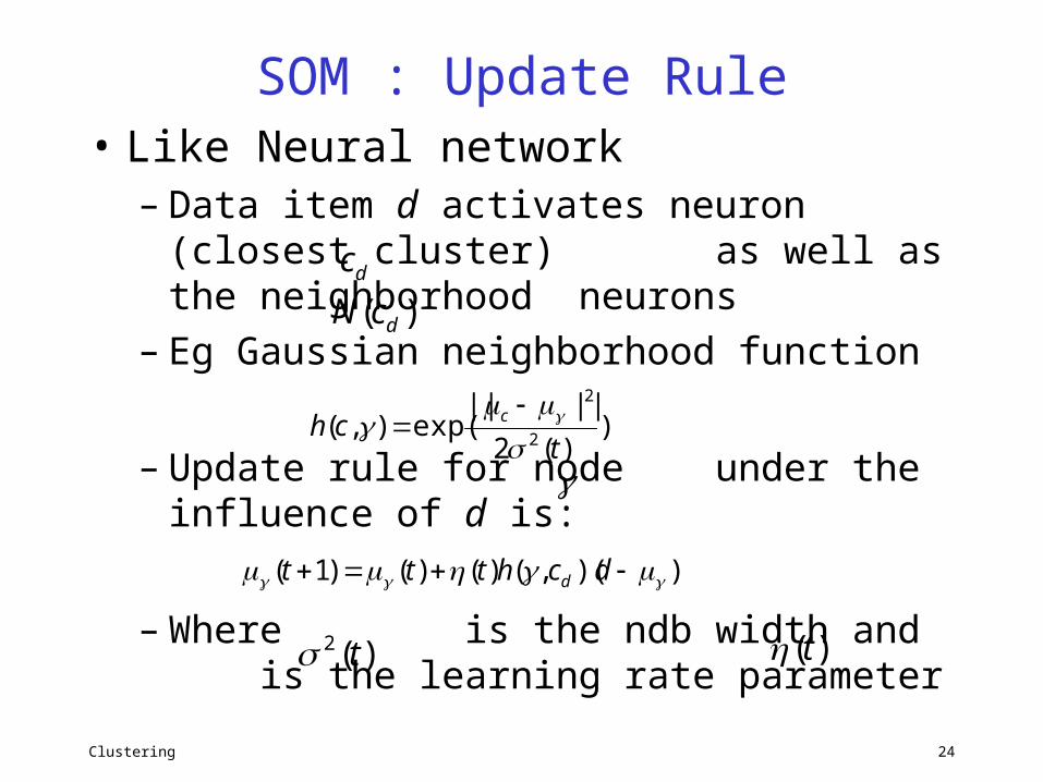
SOM : Update Rule• Like Neural network

– Data item d activates neuron (closest cluster) as well as the neighborhood neurons

– Eg Gaussian neighborhood function

– Update rule for node under the influence of d is:

– Where is the ndb width and is the learning rate parameter

dc

)( dcN

))(2

||||exp(),(

2

2

tch c

))(,()()()1( dchttt d

)(t)(2 t

Clustering 25

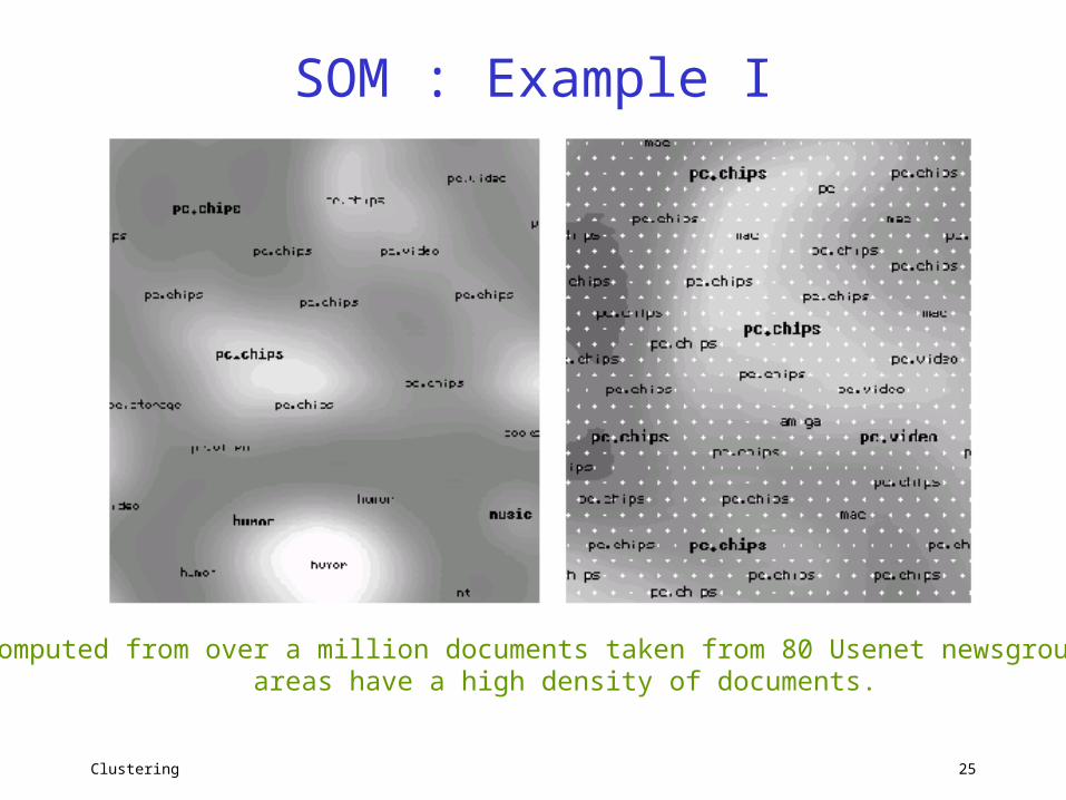
SOM : Example I

SOM computed from over a million documents taken from 80 Usenet newsgroups. Lightareas have a high density of documents.

Clustering 26

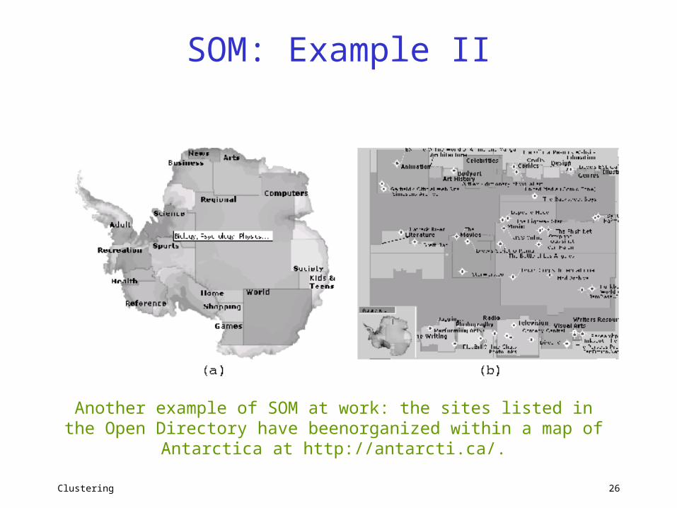
SOM: Example II

Another example of SOM at work: the sites listed in the Open Directory have beenorganized within a map of Antarctica at

http://antarcti.ca/.

Clustering 27

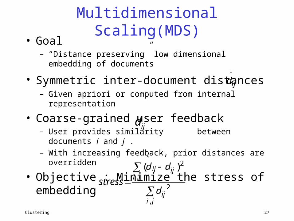
Multidimensional Scaling(MDS)• Goal

– “Distance preserving” low dimensional embedding of documents

• Symmetric inter-document distances – Given apriori or computed from internal

representation

• Coarse-grained user feedback– User provides similarity between documents i

and j .– With increasing feedback, prior distances are

overridden

• Objective : Minimize the stress of embedding

ijd

ijd

jiij

jiijij

d

dd

stress

,

2

,

2)(

Clustering 28

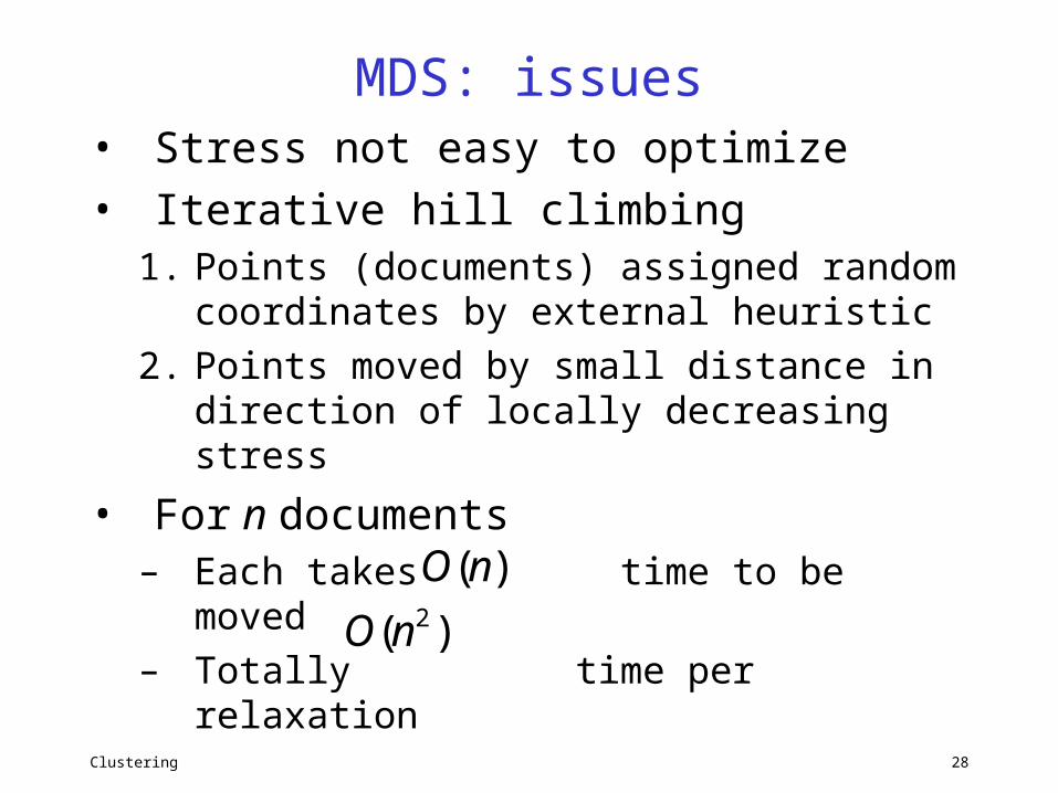
MDS: issues• Stress not easy to optimize• Iterative hill climbing

1. Points (documents) assigned random coordinates by external heuristic

2. Points moved by small distance in direction of locally decreasing stress

• For n documents – Each takes time to be moved – Totally time per relaxation

)(nO

)( 2nO

Clustering 29

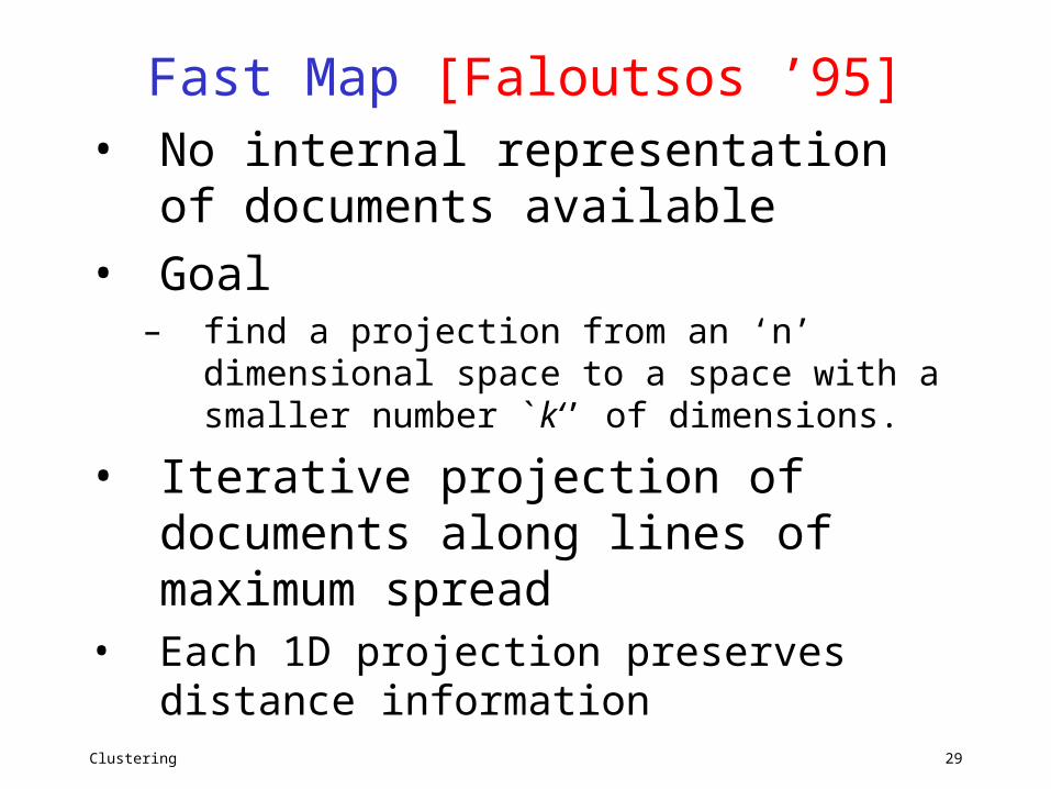
Fast Map [Faloutsos ’95]• No internal representation of

documents available• Goal

– find a projection from an ‘n’ dimensional space to a space with a smaller number `k‘’ of dimensions.

• Iterative projection of documents along lines of maximum spread

• Each 1D projection preserves distance information

Clustering 30

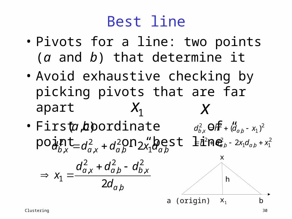
Best line• Pivots for a line: two points (a and

b) that determine it • Avoid exhaustive checking by

picking pivots that are far apart• First coordinate of point on

“best line”

ba

xbbaxa

babaxaxb

d

dddx

dxddd

,

2,

2,

2,

1

,12,

2,

2,

2

2

1x x),( ba

h

a (origin) b

x

x1

21,1

2,

2

21,

22,

2

)(

xdxdh

xdhd

baba

baxb

Clustering 31

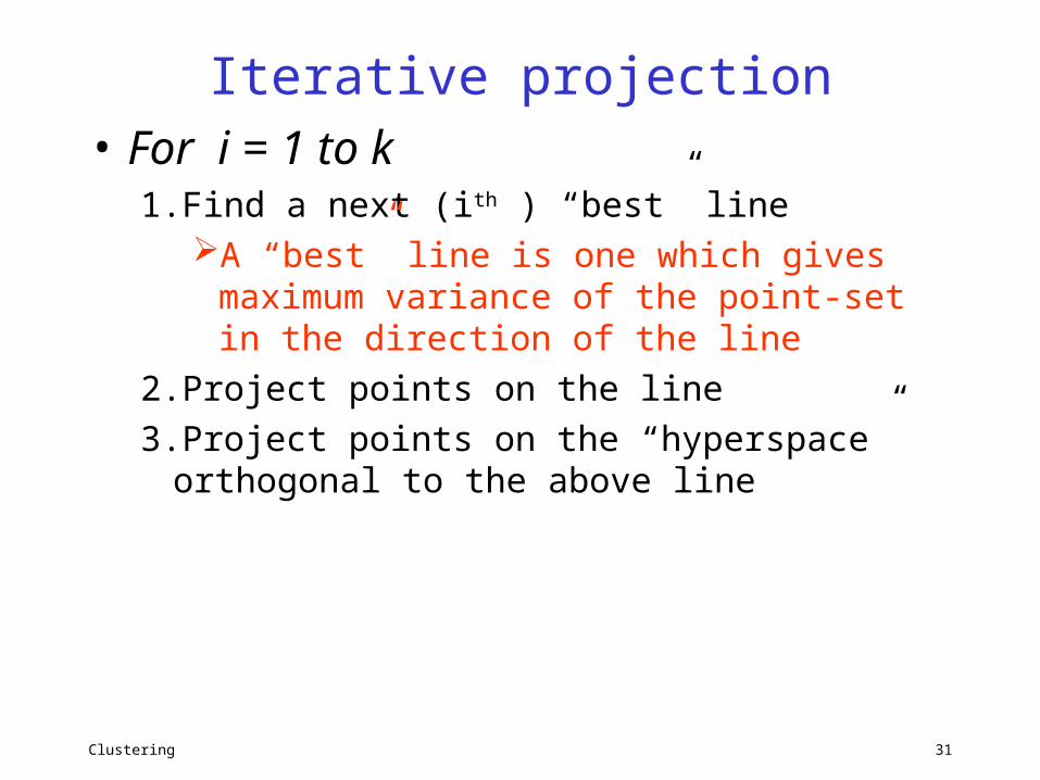
Iterative projection• For i = 1 to k

1.Find a next (ith ) “best” lineA “best” line is one which gives

maximum variance of the point-set in the direction of the line

2.Project points on the line3.Project points on the “hyperspace”

orthogonal to the above line

Clustering 32

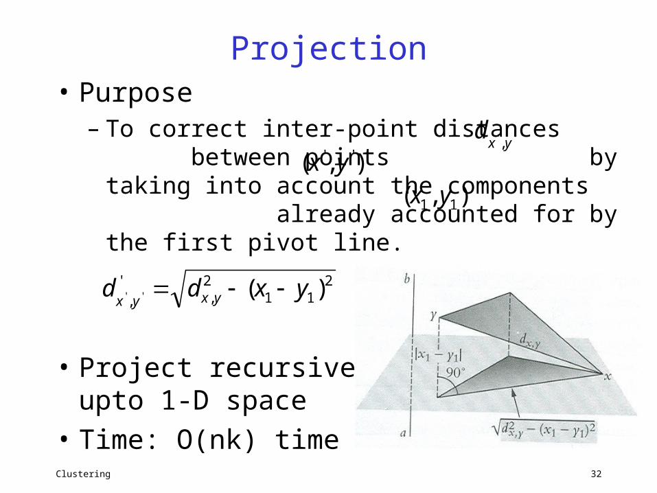
Projection• Purpose

– To correct inter-point distances between points by taking into account the components already accounted for by the first pivot line.

• Project recursively upto 1-D space

• Time: O(nk) time

211

2,

'

,)('' yxdd yxyx

),( '' yx),( 11 yx

'' , yxd

Clustering 33

Issues• Detecting noise dimensions

– Bottom-up dimension composition too slow– Definition of noise depends on application

• Running time– Distance computation dominates– Random projections– Sublinear time w/o losing small clusters

• Integrating semi-structured information– Hyperlinks, tags embed similarity clues– A link is worth a ? words

Clustering 34

Issues• Expectation maximization (EM):

– Pick k arbitrary ‘distributions’– Repeat:

• Find probability that document d is generated from distribution f for all d and f

• Estimate distribution parameters from weighted contribution of documents

Clustering 35

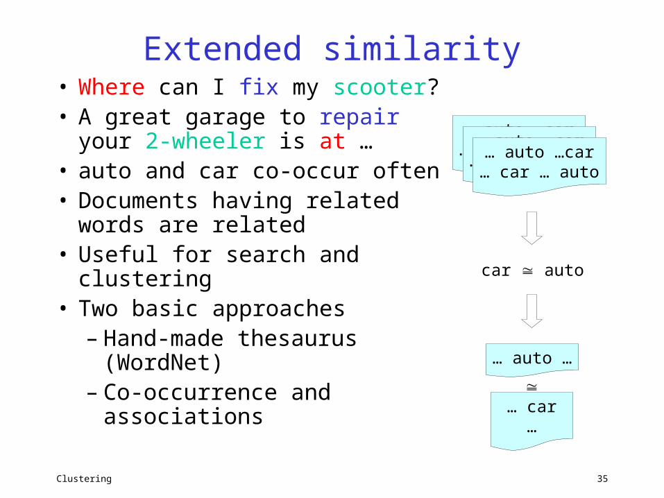
Extended similarity• Where can I fix my scooter?• A great garage to repair

your 2-wheeler is at …• auto and car co-occur often• Documents having related

words are related• Useful for search and

clustering• Two basic approaches

– Hand-made thesaurus (WordNet)

– Co-occurrence and associations

… car …

… auto …

… auto …car… car … auto… auto …car

… car … auto… auto …car… car … auto

car auto

Clustering 36

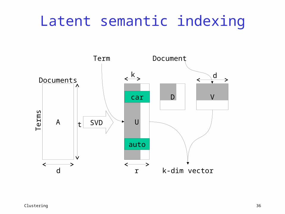
k

k-dim vector

Latent semantic indexing

A

Documents

Ter

ms

U

d

t

r

D V

d

SVD

Term Document

car

auto

Clustering 37

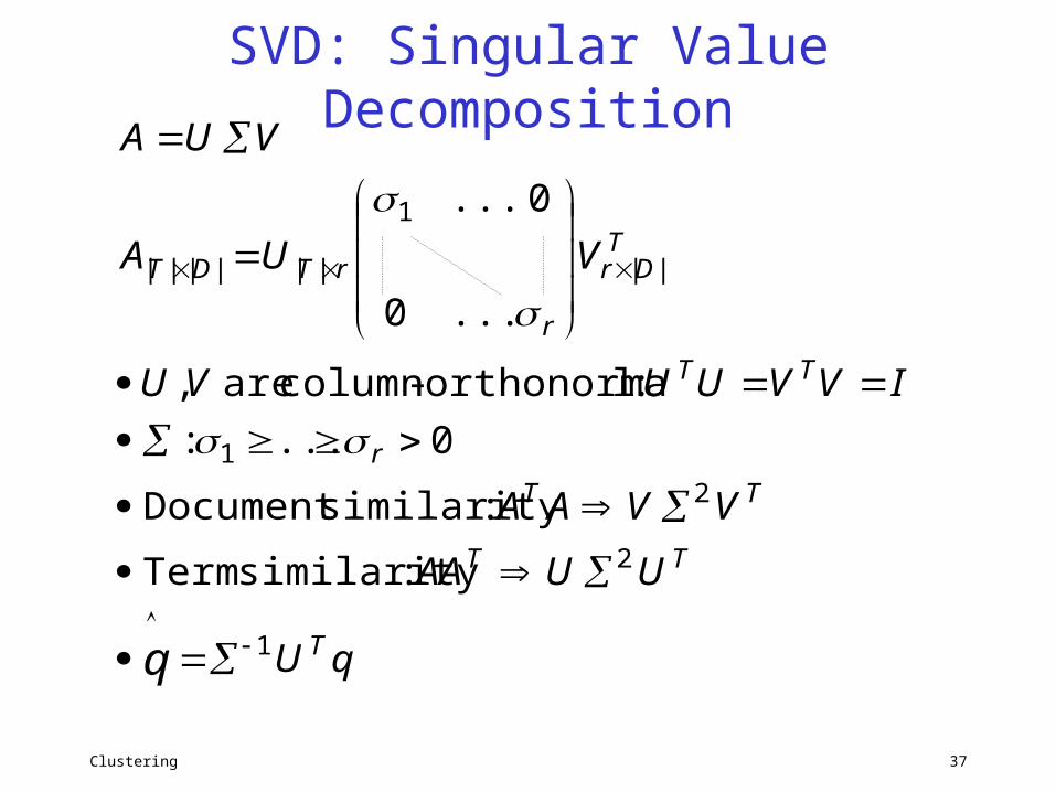
SVD: Singular Value Decomposition

qU

UUAA

VVAA

IVVUUVU

VUA

VUA

T

TT

TT

r

TT

TDr

r

rTDT

q 1

2

2

1

||

1

||||||

:similarity Term

:similarityDocument

0... :

:lorthonorma-column are ,

...0

0...

Clustering 38

Probabilistic Approaches to Clustering

• There will be no need for IDF to determine the importance of a term

• Capture the notion of stopwords vs. content-bearing words

• There is no need to define distances and similarities between entities

• Assignment of entities to clusters need not be “hard”; it is probabilistic

Clustering 39

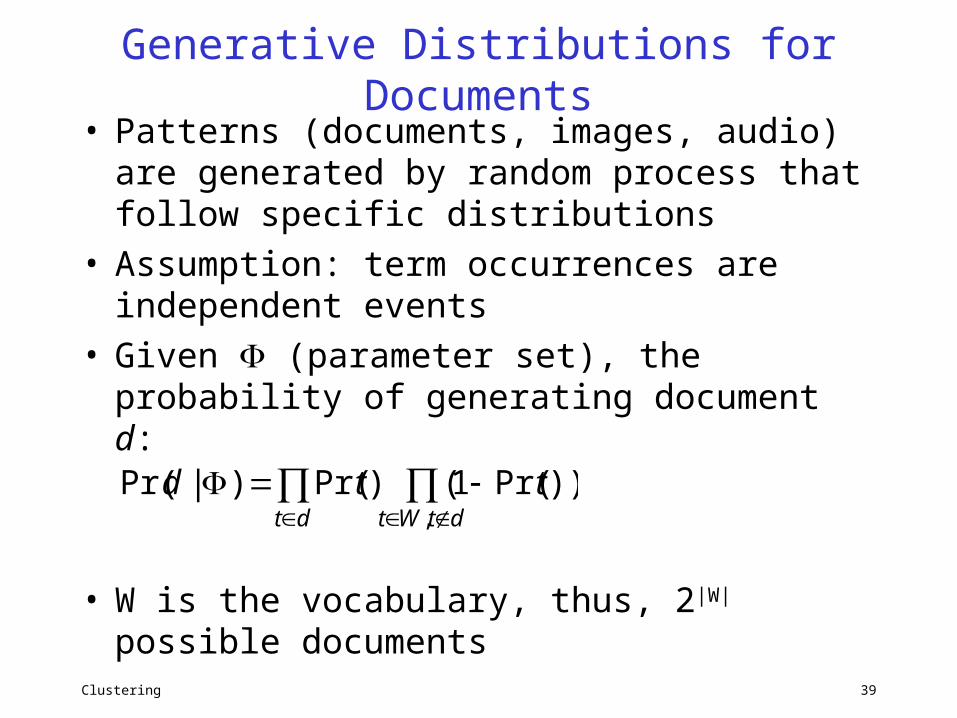
Generative Distributions for Documents

• Patterns (documents, images, audio) are generated by random process that follow specific distributions

• Assumption: term occurrences are independent events

• Given (parameter set), the probability of generating document d:

• W is the vocabulary, thus, 2|W| possible documents

dt dtWt

ttd,

))Pr(1()Pr()|Pr(

Clustering 40

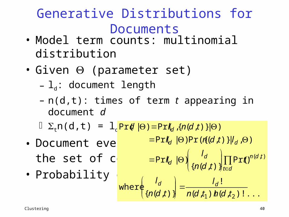
Generative Distributions for Documents

• Model term counts: multinomial distribution

• Given (parameter set)– ld: document length

– n(d,t): times of term t appearing in document d

tn(d,t) = ld

• Document event d comprises ld and the set of counts {n(d,t)}

• Probability of d :

)!...,()!,(

!

)},({ where

)Pr()},({

)|Pr(

),|)},(Pr({)|Pr(

)|)},({,Pr()|Pr(

21

),(

tdntdn

l

tdn

l

ttdn

ll

ltdnl

tdnld

dd

tdn

dt

dd

dd

d

Clustering 41

Mixture Models & Expectation Maximization (EM)

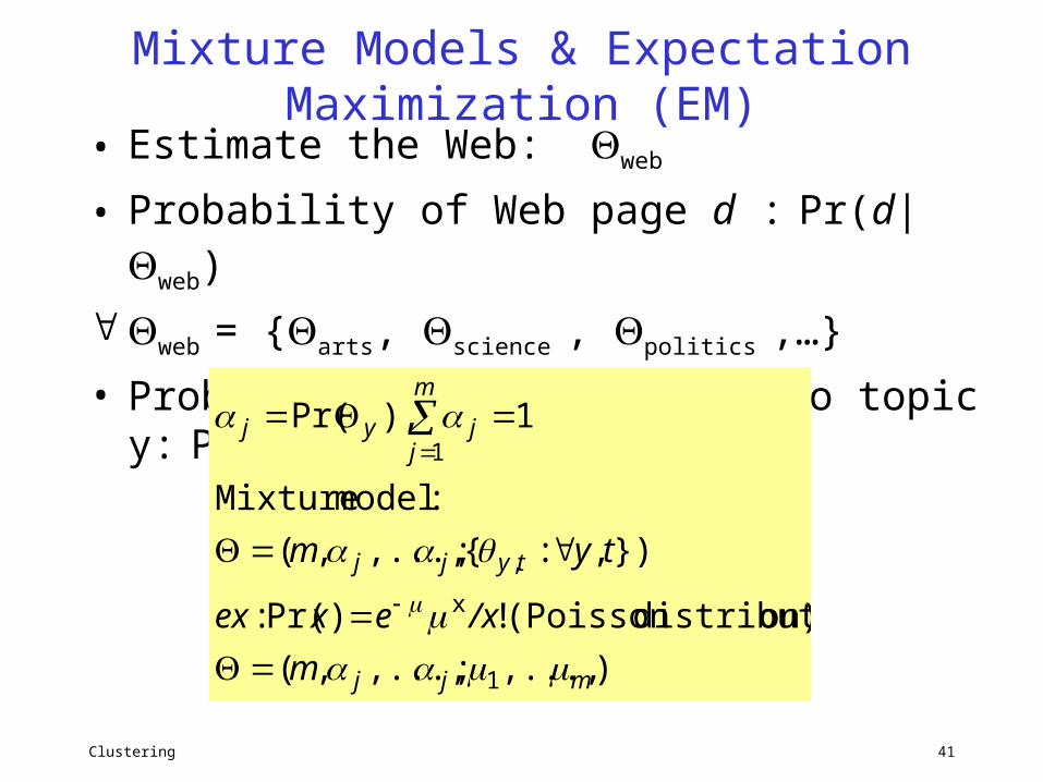
• Estimate the Web: web

• Probability of Web page d : Pr(d|web)

web = {arts, science , politics ,…}

• Probability of d belonging to topic y: Pr(d|y)

),...,;,...,,(

on)distributi(Poisson !)Pr( :

}),:{;,...,,(

:model Mixture

1),Pr(

1

x

,

1

mjj

tyjj

m

jjyj

m

/xexex

tym

Clustering 42

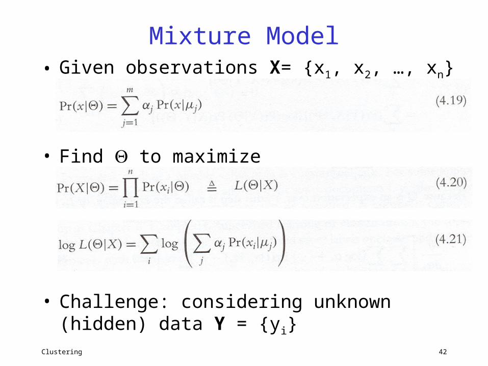
Mixture Model• Given observations X= {x1, x2, …, xn}

• Find to maximize

• Challenge: considering unknown (hidden) data Y = {yi}

Clustering 43

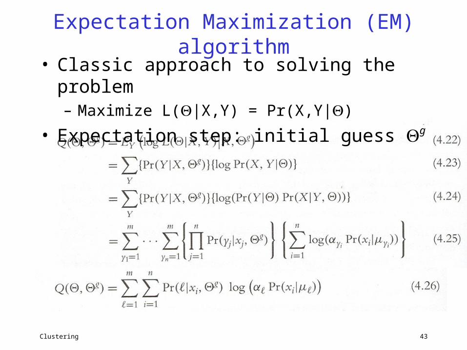
Expectation Maximization (EM) algorithm

• Classic approach to solving the problem– Maximize L(|X,Y) = Pr(X,Y|)

• Expectation step: initial guess g

Clustering 44

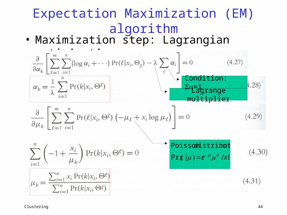
Expectation Maximization (EM) algorithm

• Maximization step: Lagrangian optimization

Lagrange multiplier

Condition: =1

!/)|Pr(

:ondistributiPoisson

xex x

Clustering 45

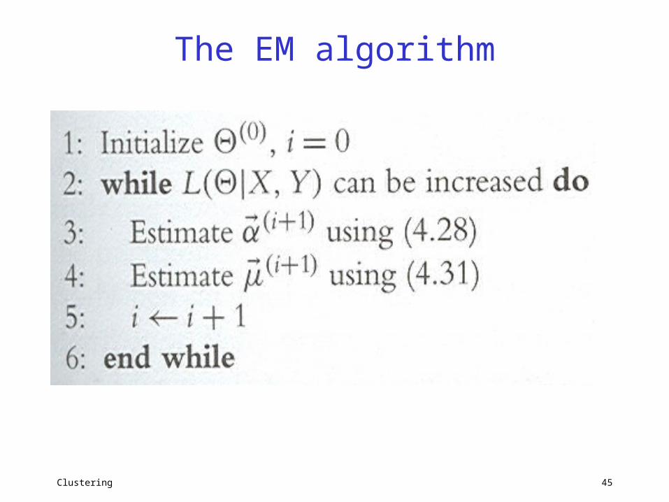
The EM algorithm

Clustering 46

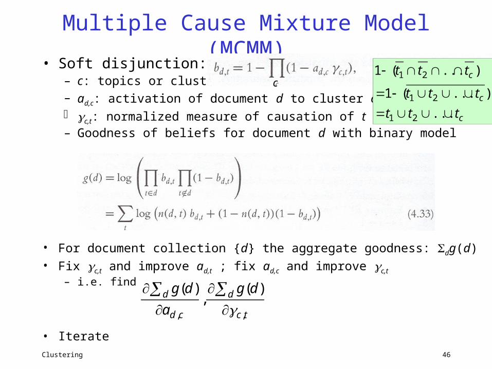
Multiple Cause Mixture Model (MCMM)

• Soft disjunction:– c: topics or clusters– ad,c: activation of document d to cluster c c,t: normalized measure of causation of t by c– Goodness of beliefs for document d with binary model

• For document collection {d} the aggregate goodness: dg(d)• Fix c,t and improve ad,t ; fix ad,c and improve c,t

– i.e. find

• Iterate

tc

d

cd

d dg

a

dg

,,

)(,

)(

c

c

c

c

ttt

ttt

ttt

...

)...(1

)...(1

21

21

21

Clustering 47

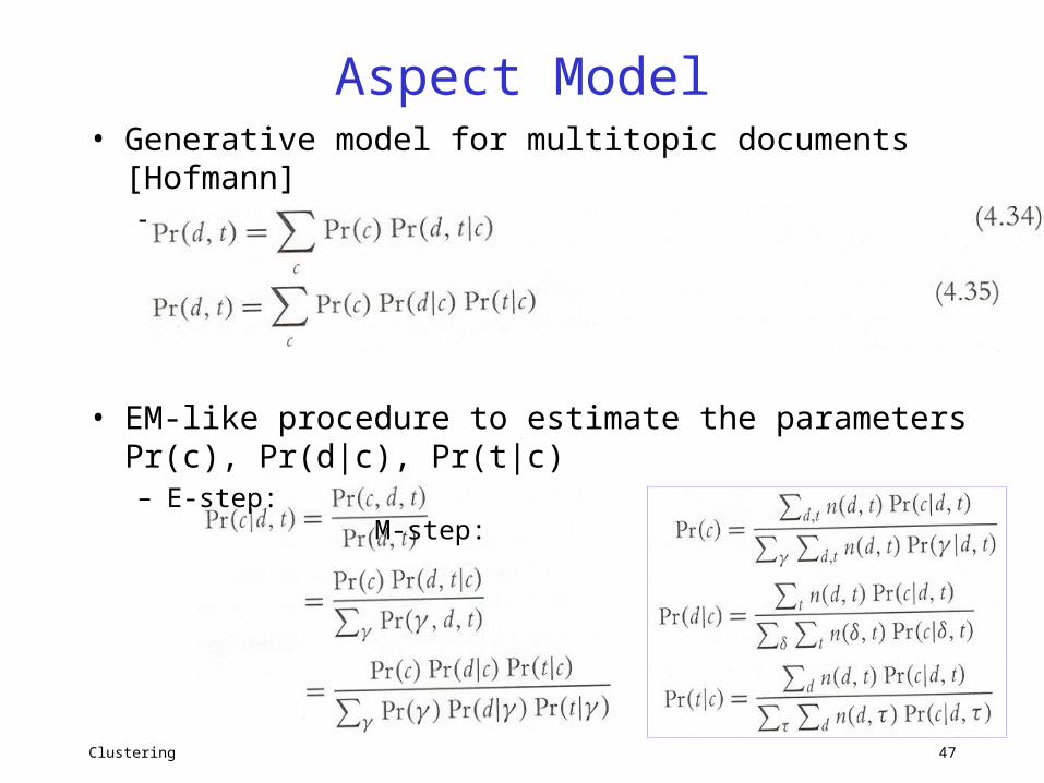
Aspect Model• Generative model for multitopic documents [Hofmann]

– Induce cluster (topic) probability Pr(c)

• EM-like procedure to estimate the parameters Pr(c), Pr(d|c), Pr(t|c)– E-step: M-step:

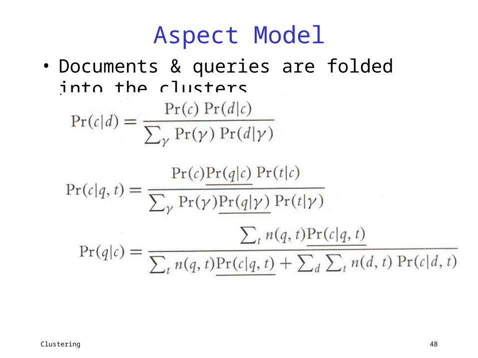
Clustering 48

Aspect Model• Documents & queries are folded into the clusters

Clustering 49

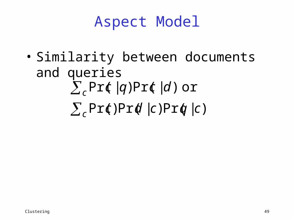
Aspect Model

• Similarity between documents and queries

c

c

cqcdc

dcqc

)|Pr()|Pr()Pr(

or )|Pr()|Pr(

Clustering 50

Batman Rambo Andre Hiver Whispers StarWarsLyleEllenJasonFredDeanKaren

Batman Rambo Andre Hiver Whispers StarWarsLyleEllenJasonFredDeanKaren

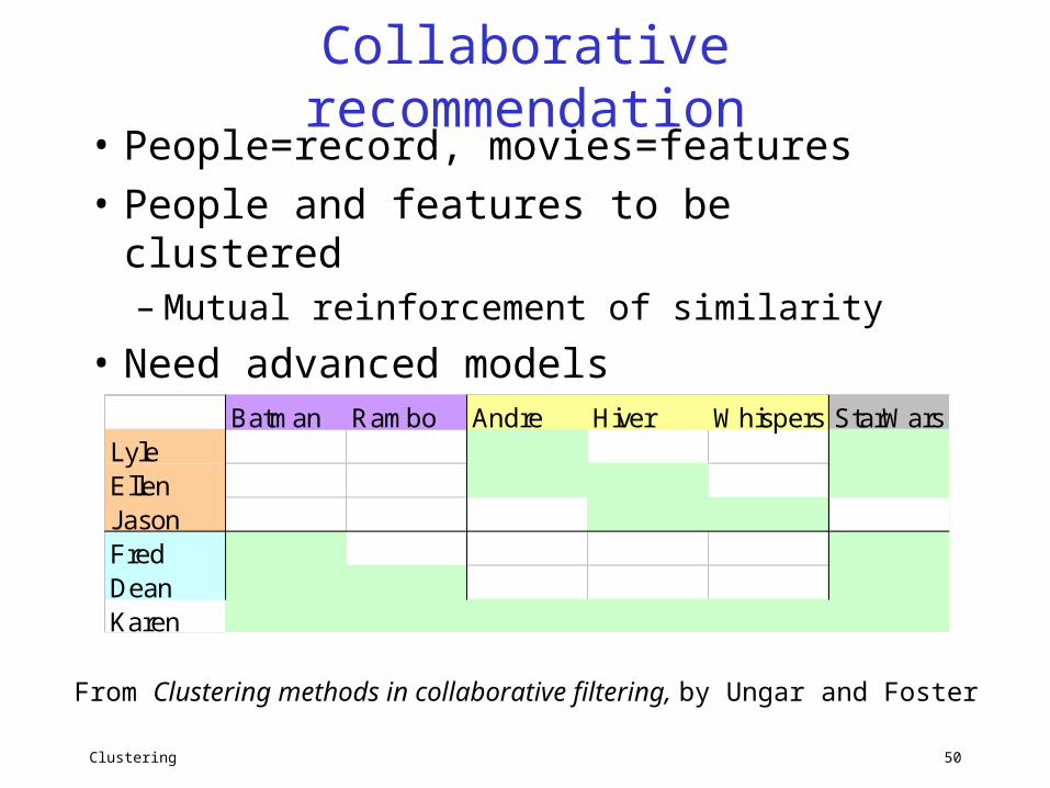
Collaborative recommendation• People=record, movies=features• People and features to be clustered

– Mutual reinforcement of similarity

• Need advanced models

From Clustering methods in collaborative filtering, by Ungar and Foster

Clustering 51

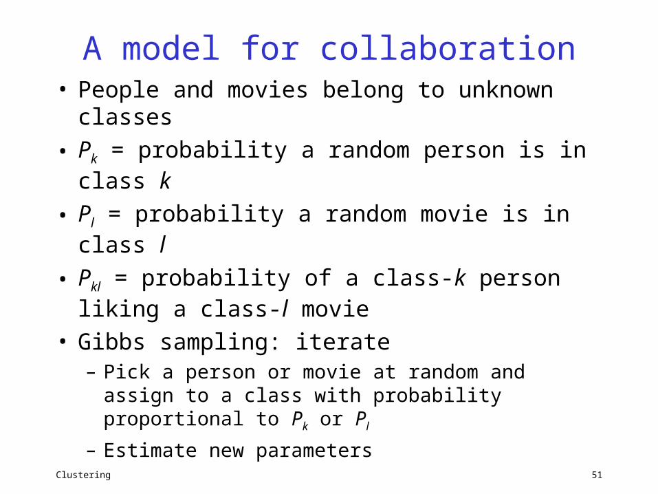
A model for collaboration• People and movies belong to unknown

classes

• Pk = probability a random person is in class k

• Pl = probability a random movie is in class l

• Pkl = probability of a class-k person liking a class-l movie

• Gibbs sampling: iterate– Pick a person or movie at random and assign to

a class with probability proportional to Pk or Pl

– Estimate new parameters

Clustering 52

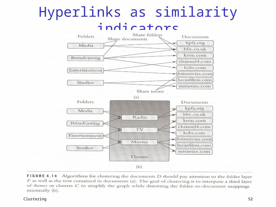
Hyperlinks as similarity indicators