Embed Size (px)
Citation preview

Introduction Trade-off Optimal UI Empirical
Lecture 6-7: Policy Design: UnemploymentInsurance and Moral Hazard
Johannes Spinnewijn
London School of Economics
Lecture Notes for Ec426
1 / 41

Introduction Trade-off Optimal UI Empirical
Topics & Question in Public Economics
Classical division in Public Economics:
Taxation: How does and should government raise revenues?
Spending: How does and should government spend revenues?
Same fundamental questions for both topics:
When and how should the government intervene?
How do government policies affect economic behavior?
2 / 41
Introduction Trade-off Optimal UI Empirical
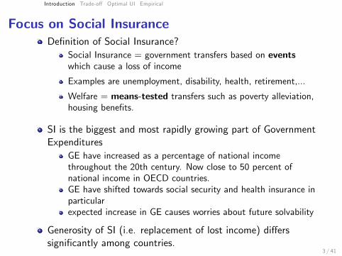
Focus on Social InsuranceDefinition of Social Insurance?
Social Insurance = government transfers based on eventswhich cause a loss of income
Examples are unemployment, disability, health, retirement,...
Welfare = means-tested transfers such as poverty alleviation,housing benefits.
SI is the biggest and most rapidly growing part of GovernmentExpenditures
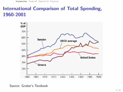
GE have increased as a percentage of national incomethroughout the 20th century. Now close to 50 percent ofnational income in OECD countries.GE have shifted towards social security and health insurance inparticularexpected increase in GE causes worries about future solvability
Generosity of SI (i.e. replacement of lost income) differssignificantly among countries.
3 / 41
Introduction Trade-off Optimal UI Empirical
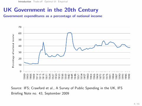
UK Government in the 20th CenturyGovernment expenditures as a percentage of national income
Source: IFS; Crawford et al., A Survey of Public Spending in the UK, IFS
Briefing Note no. 43, September 2009
4 / 41
Introduction Trade-off Optimal UI Empirical
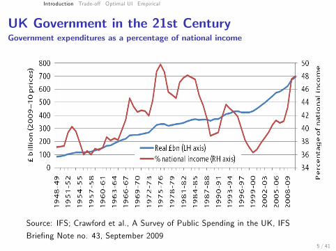
UK Government in the 21st CenturyGovernment expenditures as a percentage of national income
Source: IFS; Crawford et al., A Survey of Public Spending in the UK, IFS
Briefing Note no. 43, September 20095 / 41
Introduction Trade-off Optimal UI Empirical
International Comparison of Total Spending,1960-2001
Source: Gruber’s Textbook6 / 41
Introduction Trade-off Optimal UI Empirical
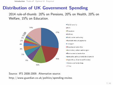
Distribution of UK Government Spending2014 rule-of-thumb: 20% on Pensions, 20% on Health, 20% onWelfare, 15% on Education.
Source: IFS 2008-2009. Alternative source:
http://www.guardian.co.uk/politics/spending-review.
7 / 41
Introduction Trade-off Optimal UI Empirical
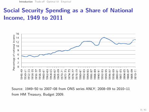
Social Security Spending as a Share of NationalIncome, 1949 to 2011
Source: 1949—50 to 2007—08 from ONS series ANLY; 2008—09 to 2010—11
from HM Treasury, Budget 2009.
8 / 41
Introduction Trade-off Optimal UI Empirical
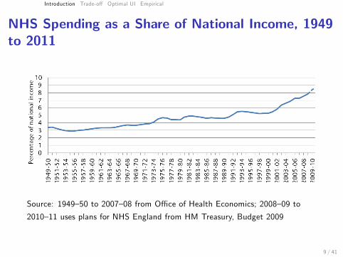
NHS Spending as a Share of National Income, 1949to 2011
Source: 1949—50 to 2007—08 from Offi ce of Health Economics; 2008—09 to
2010—11 uses plans for NHS England from HM Treasury, Budget 2009
9 / 41
Introduction Trade-off Optimal UI Empirical
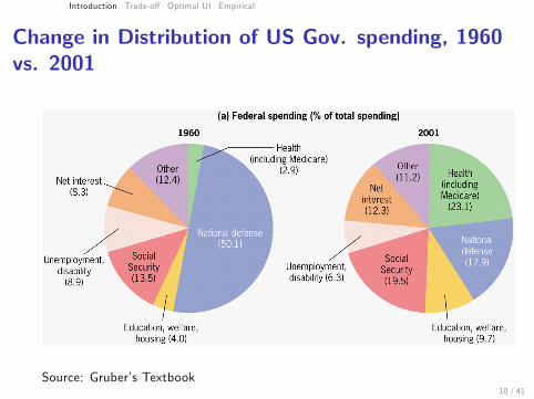
Change in Distribution of US Gov. spending, 1960vs. 2001
Source: Gruber’s Textbook10 / 41
Introduction Trade-off Optimal UI Empirical
Why have social insurance?
General motivation for insurance: pool risks of risk-averseindividuals
Unemployment: loss of earnings due to involuntaryunemployment
Health: risk of health shocks/expenses
Social security: loss of earnings at old age
But why is government intervention needed to provide thisinsurance?
First and Second Welfare Theorem optimal insuranceallocation could be decentralized
So why care about individuals not having health insurance inthe US?
11 / 41
Introduction Trade-off Optimal UI Empirical
Why have social insurance?
Typical answer is market failure due to asymmetric information
private information about actions leads to moral hazard;increase in coverage increases the probability that the riskoccurs
private information about risks leads to adverse selection;higher risk types are more likely to buy insurance
Does this provide a rational for government intervention?
in case of adverse selection it does; government has advantageover private insurers that it can mandate insurance
if governments intervene for other reasons, understanding howinterventions affect selection and incentives is essential foroptimal design
12 / 41
Introduction Trade-off Optimal UI Empirical
What else can explain government interventions?Other Market Failures
externalities, aggregate risks, redistribution, imperfectcompetition,...
Behavioral failurespeople make mistakes, do not internalize the true impact oftheir actions on themselves
Trade-off between costs and benefits of governmentintervention
1 information: how does government aggregate information onpreferences and technology to choose optimal production andallocation?
2 politicians not necessarily a benevolent planner in reality; faceincentive constraints themselves
3 why does govt. know better what’s desirable for you (e.g.wearing a seatbelt, not smoking, saving more)
13 / 41
Introduction Trade-off Optimal UI Empirical
Outline
Lecture 6-7 Unemployment Insurance & Moral Hazard
Lecture 7-8 Health Insurance & Adverse Selection
Lecture 9 Social Security
Lecture 10 Externalities
14 / 41

Introduction Trade-off Optimal UI Empirical
Approach
Integration of theory with empirical evidence to derivequantitative predictions about policy
theoretical analysis of core issues
empirical analysis of direct and indirect effects
institutional framework (incomplete)
Behavioral public economics: focus on non-standard decisionmakers where relevant
Critical about question; why government?
15 / 41

Introduction Trade-off Optimal UI Empirical
Logistics
Slides and reading list posted in advance on Frank’s website
Background textbooks:
Public Finance and Public Policy by GruberHandbook of Public Economics (recent Vol. 5 in particular)
Contact:
Email: [email protected] ce hours: Tuesday 4 - 5 (32LIF 3.24)
16 / 41
Introduction Trade-off Optimal UI Empirical
This Lecture: UI & Moral Hazard
1 Moral Hazard: Insurance vs. Incentives
2 Optimal level of UI benefits [Baily-Chetty model]
1 Model of Moral Hazard - generalizes for other applications
2 Suffi cient Statistics Approach - use of envelope conditions
3 Empirical estimation to test for optimality of program
17 / 41
Introduction Trade-off Optimal UI Empirical
Unemployment Insurance: Basic Trade-off
Insurance against unemployment
loss of current (and potentially future) earningsuninsured unemployed experience drop in consumption
If fully insured, unemployed has no (monetary) incentive tokeep/get a job
moral hazard on the job and during unemployment
Central trade-off: insurance vs. incentives ⇒ optimalgenerosity
18 / 41
Introduction Trade-off Optimal UI Empirical
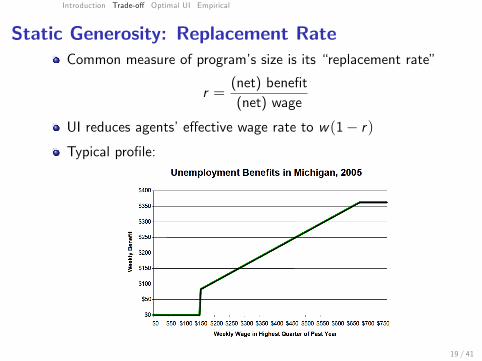
Static Generosity: Replacement RateCommon measure of program’s size is its “replacement rate”
r =(net) benefit(net) wage
UI reduces agents’effective wage rate to w(1− r)Typical profile:
19 / 41
Introduction Trade-off Optimal UI Empirical
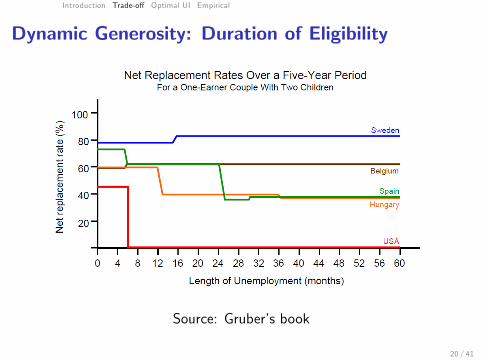
Dynamic Generosity: Duration of Eligibility
Source: Gruber’s book
20 / 41
Introduction Trade-off Optimal UI Empirical Baily-Chetty First Best Second Best
Baily-Chetty model
Canonical analysis of optimal level of UI benefits: Baily(1978)
Shows that the optimal benefit level can be expressed as a fnof a small set of parameters in a static model
Once viewed as being of limited practical relevance because ofstrong assumptions
Chetty (2006) shows formula actually applies with arbitrarychoice variables and constraints
Parameters identified by Baily are “suffi cient statistics” forwelfare analysis ⇒ robust yet simple guide for optimal policy
21 / 41
Introduction Trade-off Optimal UI Empirical Baily-Chetty First Best Second Best
Baily-Chetty model: Setup
Static model with two states: an agent is either
employed and earns wage wor unemployed and has no income
Agent is initially unemployed. Controls probability ofremaining unemployed by exerting search effort
If the agent searches at cost e, the probability of finding a jobequals π (e) with π′ > 0, π′′ < 0
22 / 41
Introduction Trade-off Optimal UI Empirical Baily-Chetty First Best Second Best
Baily-Chetty model: Setup
UI system that pays constant benefit b to unemployed agents
Benefits financed by lump sum tax τ paid by the employedagents
Govt’s balanced budget constraint:
π (e) · τ − (1− π (e)) · b = 0
Agent’s expected utility, with u(c) utility over consumption, is
π (e) u(w − τ) + (1− π (e))u(b)− e
23 / 41
Introduction Trade-off Optimal UI Empirical Baily-Chetty First Best Second Best
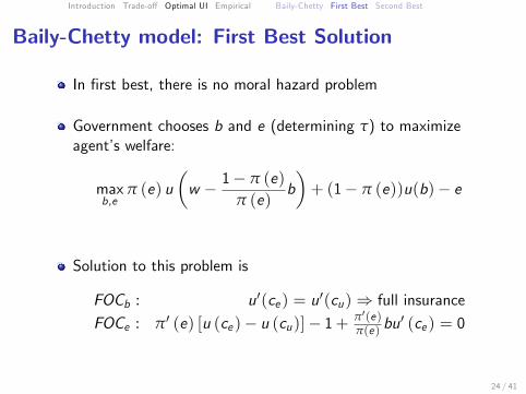
Baily-Chetty model: First Best Solution
In first best, there is no moral hazard problem
Government chooses b and e (determining τ) to maximizeagent’s welfare:
maxb,e
π (e) u(w − 1− π (e)
π (e)b)+ (1− π (e))u(b)− e
Solution to this problem is
FOCb : u′(ce ) = u′(cu)⇒ full insurance
FOCe : π′ (e) [u (ce )− u (cu)]− 1+ π′(e)π(e) bu
′ (ce ) = 0
24 / 41
Introduction Trade-off Optimal UI Empirical Baily-Chetty First Best Second Best
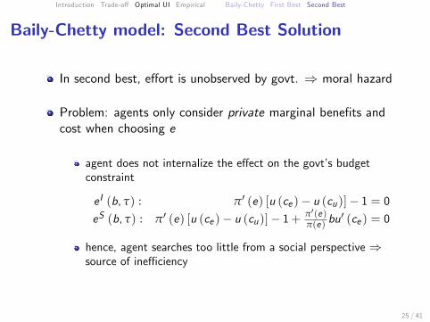
Baily-Chetty model: Second Best Solution
In second best, effort is unobserved by govt. ⇒ moral hazard
Problem: agents only consider private marginal benefits andcost when choosing e
agent does not internalize the effect on the govt’s budgetconstraint
e I (b, τ) : π′ (e) [u (ce )− u (cu)]− 1 = 0eS (b, τ) : π′ (e) [u (ce )− u (cu)]− 1+ π′(e)
π(e) bu′ (ce ) = 0
hence, agent searches too little from a social perspective ⇒source of ineffi ciency
25 / 41
Introduction Trade-off Optimal UI Empirical Baily-Chetty First Best Second Best
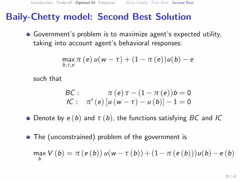
Baily-Chetty model: Second Best Solution
Government’s problem is to maximize agent’s expected utility,taking into account agent’s behavioral responses:
maxb,τ,e
π (e) u(w − τ) + (1− π (e))u(b)− e
such that
BC : π (e) τ − (1− π (e))b = 0IC : π′ (e) [u (w − τ)− u (b)]− 1 = 0
Denote by e (b) and τ (b), the functions satisfying BC and IC
The (unconstrained) problem of the government is
maxbV (b) = π (e (b)) u(w − τ (b))+ (1−π (e (b)))u(b)− e (b)
26 / 41
Introduction Trade-off Optimal UI Empirical Baily-Chetty First Best Second Best
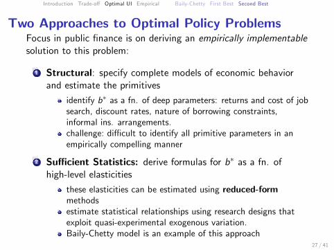
Two Approaches to Optimal Policy ProblemsFocus in public finance is on deriving an empirically implementablesolution to this problem:
1 Structural: specify complete models of economic behaviorand estimate the primitives
identify b∗ as a fn. of deep parameters: returns and cost of jobsearch, discount rates, nature of borrowing constraints,informal ins. arrangements.challenge: diffi cult to identify all primitive parameters in anempirically compelling manner
2 Suffi cient Statistics: derive formulas for b∗ as a fn. ofhigh-level elasticities
these elasticities can be estimated using reduced-formmethodsestimate statistical relationships using research designs thatexploit quasi-experimental exogenous variation.Baily-Chetty model is an example of this approach
27 / 41
Introduction Trade-off Optimal UI Empirical Baily-Chetty First Best Second Best
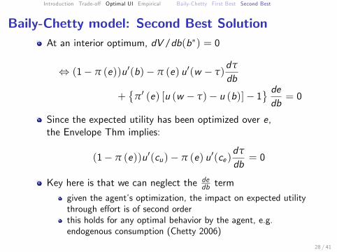
Baily-Chetty model: Second Best SolutionAt an interior optimum, dV/db(b∗) = 0
⇔ (1− π (e))u′(b)− π (e) u′(w − τ)dτ
db
+{
π′ (e) [u (w − τ)− u (b)]− 1} dedb= 0
Since the expected utility has been optimized over e,the Envelope Thm implies:
(1− π (e))u′(cu)− π (e) u′(ce )dτ
db= 0
Key here is that we can neglect the dedb term
given the agent’s optimization, the impact on expected utilitythrough effort is of second orderthis holds for any optimal behavior by the agent, e.g.endogenous consumption (Chetty 2006)
28 / 41
Introduction Trade-off Optimal UI Empirical Baily-Chetty First Best Second Best
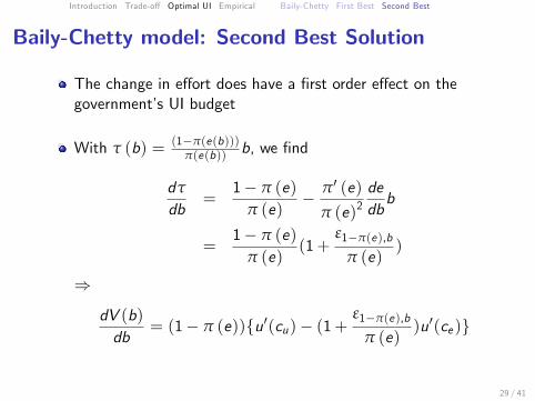
Baily-Chetty model: Second Best Solution
The change in effort does have a first order effect on thegovernment’s UI budget
With τ (b) = (1−π(e(b)))π(e(b)) b, we find
dτ
db=
1− π (e)π (e)
− π′ (e)
π (e)2dedbb
=1− π (e)
π (e)(1+
ε1−π(e),b
π (e))
⇒
dV (b)db
= (1− π (e)){u′(cu)− (1+ε1−π(e),b
π (e))u′(ce )}
29 / 41
Introduction Trade-off Optimal UI Empirical Baily-Chetty First Best Second Best
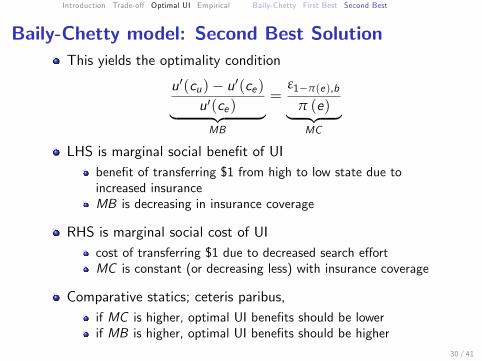
Baily-Chetty model: Second Best SolutionThis yields the optimality condition
u′(cu)− u′(ce )u′(ce )︸ ︷︷ ︸MB
=ε1−π(e),b
π (e)︸ ︷︷ ︸MC
LHS is marginal social benefit of UIbenefit of transferring $1 from high to low state due toincreased insuranceMB is decreasing in insurance coverage
RHS is marginal social cost of UIcost of transferring $1 due to decreased search effortMC is constant (or decreasing less) with insurance coverage
Comparative statics; ceteris paribus,if MC is higher, optimal UI benefits should be lowerif MB is higher, optimal UI benefits should be higher
30 / 41
Introduction Trade-off Optimal UI Empirical Baily-Chetty First Best Second Best
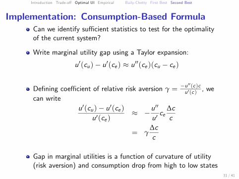
Implementation: Consumption-Based FormulaCan we identify suffi cient statistics to test for the optimalityof the current system?
Write marginal utility gap using a Taylor expansion:
u′(cu)− u′(ce ) ≈ u′′(ce )(cu − ce )
Defining coeffi cient of relative risk aversion γ = −u ′′(c )cu ′(c ) , we
can writeu′(cu)− u′(ce )
u′(ce )≈ −u
′′
u′ce
∆cc
= γ∆cc
Gap in marginal utilities is a function of curvature of utility(risk aversion) and consumption drop from high to low states
31 / 41
Introduction Trade-off Optimal UI Empirical Baily-Chetty First Best Second Best
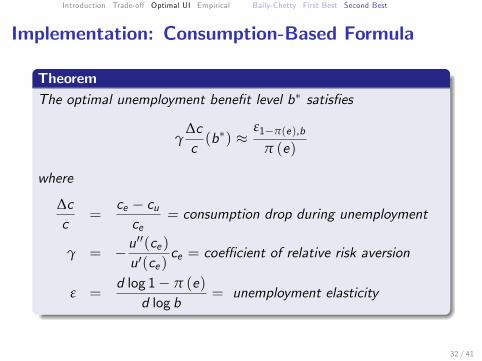
Implementation: Consumption-Based Formula
TheoremThe optimal unemployment benefit level b∗ satisfies
γ∆cc(b∗) ≈
ε1−π(e),b
π (e)
where
∆cc
=ce − cuce
= consumption drop during unemployment
γ = −u′′(ce )u′(ce )
ce = coeffi cient of relative risk aversion
ε =d log 1− π (e)
d log b= unemployment elasticity
32 / 41
Introduction Trade-off Optimal UI Empirical MH Elasticity Consumption Smoothing
Estimating the Moral Hazard Cost
Lots of empirical work on labor supply effect of socialinsurance. Overview by Krueger and Meyer (2002)
Early literature used cross-sectional variation in replacementrates. Problem: this implies a comparison of high and lowwage earners, whose employment prospects may be verydifferent!
This gave way in late 80s/early 90s to modern methods usingmore exogenous variation/quasi-experiments
difference in UI generosity across states, across time, acrossgroup...state experiments with UI bonuses (Meyer 1995)
Evidence suggests elasticity of around 0.5.
33 / 41
Introduction Trade-off Optimal UI Empirical MH Elasticity Consumption Smoothing
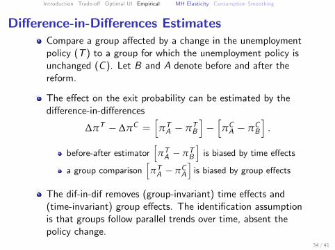
Difference-in-Differences EstimatesCompare a group affected by a change in the unemploymentpolicy (T ) to a group for which the unemployment policy isunchanged (C ). Let B and A denote before and after thereform.
The effect on the exit probability can be estimated by thedifference-in-differences
∆πT − ∆πC =[πTA − πTB
]−[πCA − πCB
].
before-after estimator[πTA − πTB
]is biased by time effects
a group comparison[πTA − πCA
]is biased by group effects
The dif-in-dif removes (group-invariant) time effects and(time-invariant) group effects. The identification assumptionis that groups follow parallel trends over time, absent thepolicy change.
34 / 41
Introduction Trade-off Optimal UI Empirical MH Elasticity Consumption Smoothing
35 / 41
Introduction Trade-off Optimal UI Empirical MH Elasticity Consumption Smoothing
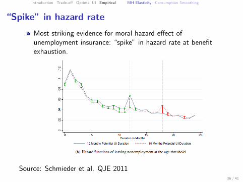
“Spike” in hazard rate
Most striking evidence for moral hazard effect ofunemployment insurance: “spike” in hazard rate at benefitexhaustion.
Source: Schmieder et al. QJE 201136 / 41
Introduction Trade-off Optimal UI Empirical MH Elasticity Consumption Smoothing
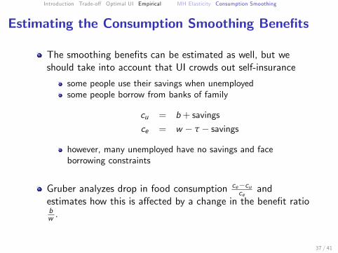
Estimating the Consumption Smoothing Benefits
The smoothing benefits can be estimated as well, but weshould take into account that UI crowds out self-insurance
some people use their savings when unemployedsome people borrow from banks of family
cu = b+ savings
ce = w − τ − savings
however, many unemployed have no savings and faceborrowing constraints
Gruber analyzes drop in food consumption ce−cuce
andestimates how this is affected by a change in the benefit ratiobw .
37 / 41

Introduction Trade-off Optimal UI Empirical MH Elasticity Consumption Smoothing
Simulated InstrumentsSame problem: the difference in consumption drop forindividuals with high and low replacement rates is not onlydue to the replacement rate differential.
Alternative solution: Simulated Instrumentstake a representative subsample of individuals S sub
for each individual i in state j at year t in the original samplecalculate the subsample’s average replacement rate if allindividuals of the subsample had lived in state j at year t(
bw
)simulatedj ,t
= ΣsεS subbsimulateds ,j ,t
ws
use(bw
)simulatedj ,t
as an instrument for(bw
)i ,j ,t
The approach exploits only variation in the generosity of thestate UI system over time (∼ difference-in-difference).Underlying the identification is a similar parallel-trendsassumption.
38 / 41

Introduction Trade-off Optimal UI Empirical MH Elasticity Consumption Smoothing
Estimating the Insurance ValueGruber runs IV regression(
ce − cuce
)i ,j ,t
= β1 + β2
(bw
)i ,j ,t+ β3δj + β4τt + εi
and finds:
β1 = 0.24, β2 = −0.28without UI, cons drop would be about 24%a 10 pp increase in UI replacement rate causes 2.8 ppreduction in cons. drop.with current replacement rate (b/w = 0.5), cons drop isabout 10%
Is current level optimal?
γ× 10% ?= 0.5
39 / 41
Introduction Trade-off Optimal UI Empirical MH Elasticity Consumption Smoothing
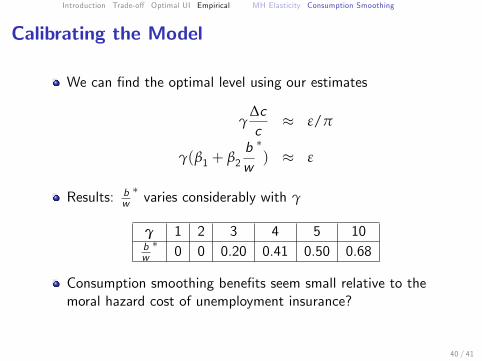
Calibrating the Model
We can find the optimal level using our estimates
γ∆cc≈ ε/π
γ(β1 + β2bw
∗) ≈ ε
Results: bw∗varies considerably with γ
γ 1 2 3 4 5 10bw∗
0 0 0.20 0.41 0.50 0.68
Consumption smoothing benefits seem small relative to themoral hazard cost of unemployment insurance?
40 / 41
Introduction Trade-off Optimal UI Empirical MH Elasticity Consumption Smoothing
SummaryPolicy maker faces trade-off between the provision ofinsurance and the provision of incentives.
Simple model with search efforts can capture this trade-off.Model generalizes for other behavioral responses like saving,moral hazard on the job, quality of job matches,...
if behavior is optimal, change in behavior has second-ordereffect on welfareonly the effect on the government’s budget constraint isimportant and this is captured by the unemploymentprobability
Empirical evidence suggests that job seekers are quiteresponsive to monetary incentives, implying that consumptionbenefits need to be large to justify generous unemploymentbenefits
41 / 41