Lecture 6 Consumer Choice - Lakehead Universityflash.lakeheadu.ca/~kyu/B5017/B6.pdf · (inferior goods), or vertical (table ... Normal, and Inferior Goods Observations during the

Lecture 6 Consumer ChoiceBusiness 5017 Managerial Economics

Kam Yu

Fall 2013

Outline

1 Rational ChoiceConsumption DecisionsMarket Demand

2 Consumers’ ResponsivenessPriceApplicationsIncomeSubstitutes and Complements

3 Lagged Demands, Network Effects, and Rational Addiction

Kam Yu (LU) Lecture 6 Consumer Choice Fall 2013 2 / 28

Rational Choice Consumption Decisions

Recap of Rational Behaviours

In Lecture 2, we assume that a rational consumer behaves according tosome rules:

1 Completeness: Given two choices, a consumer is able to decide sheprefers one or the other, or she is indifferent between them.

2 Transitivity: If a consumer prefers A to B and B to C , then she mustprefer A to C .

3 More is Better: There is always something that a consumer wantsmore. That is, we are never totally satisfied with what we have.

From these assumptions, economists use a mathematical trick to representa consumer’s welfare by a utility function.



Utility Functions

A utility function relates a consumption bundle to a number. Example:

Assume that Anna buys only two goods, Coke (c) and hot dog (h).

A consumption bundle is a list of the quantities of the goods, (c , h).

The utility function f isf (c , h) = u,

where u is a number indicating the utility level.

Suppose that f (2, 1) = 49, that is, two Cokes and one hot dog givethe utility level of 49. On the other hand, f (1, 2) = 55.

Since 55 > 49, hungry Anna prefers one Coke and two hot dogs (1, 2)to two Cokes and one hot dog (2, 1).



Marginal Utility

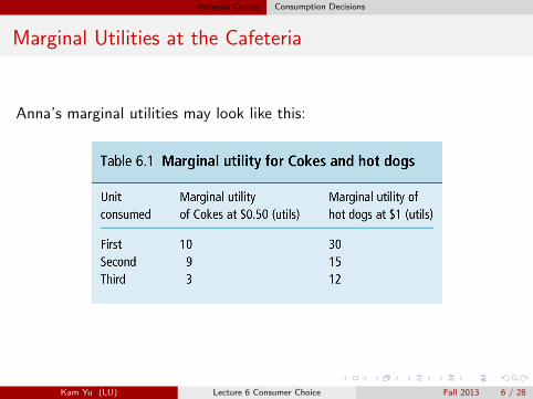
Suppose Anna has one Coke and two hot dogs, with utilityf (1, 2) = 55.

What if we buy her one more Coke?

Her utility will increase, say, to f (2, 2) = 64.

Given that she’s already had (c, h) = (1, 2), the extra utility of onemore Coke is 64− 55 = 9.

We call this the marginal utility of Coke when she has consumed onealready.

As Anna buys more Cokes or hot dogs, utility from the additionalconsumption becomes smaller and smaller. This is called diminishingmarginal utility.



Marginal Utilities at the Cafeteria

Anna’s marginal utilities may look like this:



Optimal Consumption Bundle

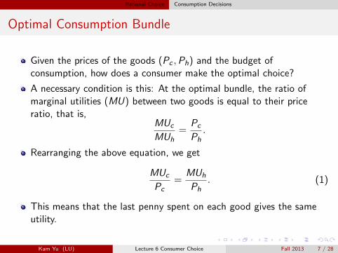
Given the prices of the goods (Pc ,Ph) and the budget ofconsumption, how does a consumer make the optimal choice?

A necessary condition is this: At the optimal bundle, the ratio ofmarginal utilities (MU) between two goods is equal to their priceratio, that is,

MUc

MUh=

Pc

Ph.

Rearranging the above equation, we get

MUc

Pc=

MUh

Ph. (1)

This means that the last penny spent on each good gives the sameutility.



Two Hot Dogs with a Medium Diet Coke Please

Why does Equation (1) have to hold at the optimal bundle?

Imagine it does not, say

MUc

Pc>

MUh

Ph.

This means that the last penny spent on Coke gives a higher marginalutility than that of hot dog.

The consumer can be better off by shifting the last penny spent onhot dog to Coke.

The opposite is true if the inequality goes in the other direction.

Conclusion: utility is maximized when equality holds.



Law of Demand

What if on the next day the Cafeteria increase the price of Coke?

Since Pc is now higher, at theold optimal bundle,

MUc

Pc<

MUh

Ph.

Now Anna is better off byspending less on Coke and moreon hot dog.

In other words, quantitydemanded for Coke will goesdown.

We have proven the law ofdemand for one consumer.


Rational Choice Market Demand

What About the Market Demand Curve?

At any given price, we need to add up the quantity demanded from all theconsumers:


Consumers’ Responsiveness Price

Price Elasticity of Demand

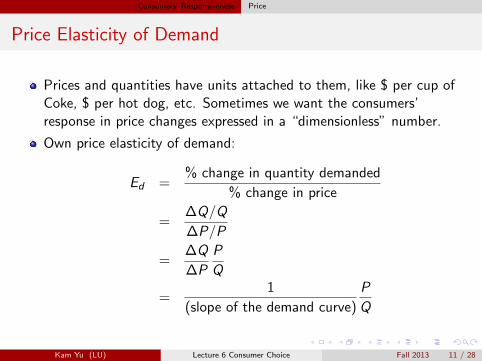
Prices and quantities have units attached to them, like $ per cup ofCoke, $ per hot dog, etc. Sometimes we want the consumers’response in price changes expressed in a “dimensionless” number.

Own price elasticity of demand:

Ed =% change in quantity demanded

% change in price

=∆Q/Q

∆P/P

=∆Q

∆P

P

Q

=1

(slope of the demand curve)

P

Q



Some Elasticities

Technically, Ed is always negative because of the law of demand.Thus a lot of economists only care about the absolute value, |Ed |,that is, the value without the negative sign.

Some results from empirical studies:

Good or Service ElasticityCigarettes 0.42Salmon 2.47Gasoline 0.50Chicken 1.67Peak hour bus services 0.23



Some Definitions

The elasticity of demand measures the degree the responsiveness of theconsumers. Three distinct cases:

1 inelastic: 0 ≤ Ed < 1

2 unitary elastic: Ed = 1

3 elastic: Ed > 1

Some extreme cases:

When a good or service is needed at a certain quantity no matterwhat the price is, the demand curve is vertical and Ed = 0.

In a perfect competitive market, each producer faces a horizontaldemand curve. That is, demand is perfectly elastic, Ed →∞.



Straight-Line Demand Curve

Elasticity along a straight-line demand curve:

Although the demand curve has the same slope everywhere, P and Qare different at different points.

Elastic range: The upper part has high prices and small quantities,therefore demand is elastic (Ed > 1).

Inelastic range: The lower part has low prices and large quantities,therefore demand is inelastic (Ed < 1).

Unitary elasticity: The two parts are separated by a point withEd = 1.



Straight-Line Demand Curve


Consumers’ Responsiveness Applications

Maximizing Revenue

Question: A firm facing a downward sloping demand curve wants to paydown debt and need cash, the business managers wants to maximize salesrevenues (R = PQ). What price should she set?

At one extreme, price is set too high and quantity demanded is zero.

At the other extreme a zero price will sell a lot of goods but norevenue as well.

Answer: The manager should set the price at the level such thatEd = 1.

Why? At a point in the elastic range, Ed > 1 so that a 1% price cutwill trigger a more than 1% increase in sales. Revenue increases.

At a point in the inelastic range, Ed < 1 so that a 1% price hike willtrigger a less than 1% decrease in sales. Revenue increases.



Need Cash?



Fat Tax

Some U.S. state governments are consider a “fat tax” on fatty foodand sugary drink as a tool to reduce the obesity rate.

The effectiveness of the tax critically depends on the elasticity ofdemand on those food.

Empirical studies have found that the estimated Ed for sodabeverages ranges from 0.78 to 1.22.

Other studies suggest that a fat tax has small impacts on the averageweight of Americans.



Easy Ways to Lose Weight? Stay in School

Economists Jay Bhattacharya and Neeraj Sood find that obesity hassomething to do with studying.


Consumers’ Responsiveness Income

Income and Demand

Instead of price, we can find the relation between income and quantitydemanded for a good or service, assuming that price remains the same.



Engel Curve

The Engel curve can slope upward (normal goods), downward(inferior goods), or vertical (table salt).

they can even change direction: a good can be normal at low incomelevel but becomes inferior at high income level, can you give anexample?



Income Elasticity of Demand

Ei =% change in quantity demanded

% change in income

=∆Q/Q

∆M/M

=∆Q

∆M

M

Q

=1

(slope of the Engel curve)

M

Q

Classification of goods:

inferior goods: Ei < 0

necessities: 0 ≤ Ei ≤ 1

luxuries: Ei > 1



Luxury, Normal, and Inferior Goods

Observations during the 2008 recession:


Consumers’ Responsiveness Substitutes and Complements

Substitutes and Complements

Two goods are substitutes if the price of one good goes up result in anincrease in demand for the other good. Examples:

Zippers and buttons

Butter and margarine

Natural gas and fuel oil

Pork and chicken

Two goods are complements if the price of one good goes up result in andecrease in demand for the other good. Examples:

Movie tickets and restaurant meals

Lettuce and salad dressing

Blue-ray players and HDTV


Consumers’ Responsiveness Substitutes and Complements

Cross-Price Elasticity of Demand

The cross-price elasticity of two goods X and Y is defined as

EXY =% change in quantity demanded for X

% change in price of Y

=∆QX/QX

∆PY /PY

=∆QX

∆PY

PY

QX


Lagged Demands, Network Effects, and Rational Addiction

Lagged Demands

Definition: Consumption is intertemporal in nature. Demand of agood in the future depends on the current demand.

This applies to products that are addictive or habitual.

Firms have different pricing strategies in selling these product. Theyoften offer a very low price for new customers and charge the“normal” price after a kick-in period.

Examples:Tobacco companies tried to often free cigarettes to new smokers.Cable, digital phone, and Internet services providers offer low pricepackages for the first six months.Subprime mortgage lenders offered low teaser rates for the first twoyears.

In business, this leads to the problem of asset specificity. For example,utility companies usually sign long-term contracts with miningcompanies before building a coal-fired power plant near a mine.



Network Effects

Definition: The value of a product depends on the total number ofusers.

The effect occurs most commonly in IT products which rely onnetworking: telephone, telex, fax, the Internet, Skype, Facebook.

Firms face the critical mass problem in product development. Thevalue of a smartphone depends on the number of apps available. Butsoftware developers do not want to write apps for systems with fewusers.

Economist Edward Glaeser suggests that people want to live in bigcities because of the positive network externality of knowledge andidea exchanges.



World Mobile Phone Market


Documents

Lecture 6 Consumer Choice - Lakehead Universityflash.lakeheadu.ca/~kyu/B5017/B6.pdf · (inferior goods), or vertical (table ... Normal, and Inferior Goods Observations during the