Embed Size (px)
Citation preview
VelocityRate of ChangeThe Derivative
Lecture 7: Velocity, Rate of Change, and the Derivative
VelocityAverage VelocityInstantaneous VelocityExample 25 – Computing Velocities from a GraphEstimating Slope by Averaging – Straddling
Rate of ChangeAverage Rate of ChangeInstantaneous Rate of ChangeExample 26 – Rate of Change of Area
The DerivativeThe Derivative at a PointExamples of DerivativesExample 27 – Calculating a Derivative at a Point
Clint Lee Math 112 Lecture 7: Velocity and Rate of Change 1/26
VelocityRate of ChangeThe Derivative
Average VelocityInstantaneous VelocityExample 25 – Computing Velocities from a GraphEstimating Slope by Averaging – Straddling
Representing Motion
Consider an object moving along astraight line. Suppose that the position ofthe object along the line relative to someorigin is given by s = f (t), where s is a realnumber representing the distance,positive to the right and negative to theleft, from the origin. The function f is theposition function of the object. Themotion of the object can be represented ina diagram like this.
Clint Lee Math 112 Lecture 7: Velocity and Rate of Change 2/26
VelocityRate of ChangeThe Derivative
Average VelocityInstantaneous VelocityExample 25 – Computing Velocities from a GraphEstimating Slope by Averaging – Straddling
Representing Motion
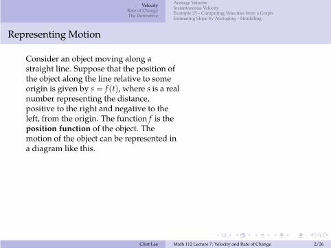
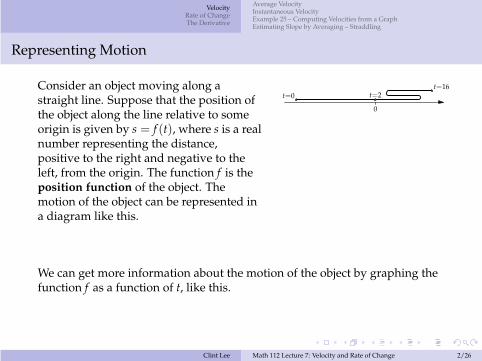
Consider an object moving along astraight line. Suppose that the position ofthe object along the line relative to someorigin is given by s = f (t), where s is a realnumber representing the distance,positive to the right and negative to theleft, from the origin. The function f is theposition function of the object. Themotion of the object can be represented ina diagram like this.
0
t=0t=16
t=2
Clint Lee Math 112 Lecture 7: Velocity and Rate of Change 2/26
VelocityRate of ChangeThe Derivative
Average VelocityInstantaneous VelocityExample 25 – Computing Velocities from a GraphEstimating Slope by Averaging – Straddling
Representing Motion
Consider an object moving along astraight line. Suppose that the position ofthe object along the line relative to someorigin is given by s = f (t), where s is a realnumber representing the distance,positive to the right and negative to theleft, from the origin. The function f is theposition function of the object. Themotion of the object can be represented ina diagram like this.
0
t=0t=16
t=2
We can get more information about the motion of the object by graphing thefunction f as a function of t, like this.
Clint Lee Math 112 Lecture 7: Velocity and Rate of Change 2/26
VelocityRate of ChangeThe Derivative
Average VelocityInstantaneous VelocityExample 25 – Computing Velocities from a GraphEstimating Slope by Averaging – Straddling
Representing Motion
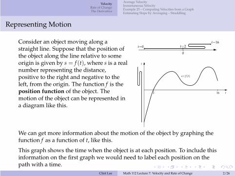
Consider an object moving along astraight line. Suppose that the position ofthe object along the line relative to someorigin is given by s = f (t), where s is a realnumber representing the distance,positive to the right and negative to theleft, from the origin. The function f is theposition function of the object. Themotion of the object can be represented ina diagram like this.
0
t=0t=16
t=2
t
s
s= f (t)
2 16
We can get more information about the motion of the object by graphing thefunction f as a function of t, like this.
This graph shows the time when the object is at each position. To include thisinformation on the first graph we would need to label each position on thepath with a time.
Clint Lee Math 112 Lecture 7: Velocity and Rate of Change 2/26
VelocityRate of ChangeThe Derivative
Average VelocityInstantaneous VelocityExample 25 – Computing Velocities from a GraphEstimating Slope by Averaging – Straddling
Average Velocity
The velocity of a moving object is the displacement or change in positionper unit time. Velocity can be positive, negative, or zero (even if the body ismoving). The speed of the object is the total distance traveled per unit time,which can be different than the velocity and is always positive.
Clint Lee Math 112 Lecture 7: Velocity and Rate of Change 3/26
VelocityRate of ChangeThe Derivative
Average VelocityInstantaneous VelocityExample 25 – Computing Velocities from a GraphEstimating Slope by Averaging – Straddling
Average Velocity
The velocity of a moving object is the displacement or change in positionper unit time. Velocity can be positive, negative, or zero (even if the body ismoving). The speed of the object is the total distance traveled per unit time,which can be different than the velocity and is always positive.
The average velocity of the object whose position is given by s = f (t) overthe time interval between t = t1 and t = t2 is
vave
Clint Lee Math 112 Lecture 7: Velocity and Rate of Change 3/26
VelocityRate of ChangeThe Derivative
Average VelocityInstantaneous VelocityExample 25 – Computing Velocities from a GraphEstimating Slope by Averaging – Straddling
Average Velocity
The velocity of a moving object is the displacement or change in positionper unit time. Velocity can be positive, negative, or zero (even if the body ismoving). The speed of the object is the total distance traveled per unit time,which can be different than the velocity and is always positive.
The average velocity of the object whose position is given by s = f (t) overthe time interval between t = t1 and t = t2 is
vave =f (t2) − f (t1)
t2 − t1
Clint Lee Math 112 Lecture 7: Velocity and Rate of Change 3/26
VelocityRate of ChangeThe Derivative
Average VelocityInstantaneous VelocityExample 25 – Computing Velocities from a GraphEstimating Slope by Averaging – Straddling
Average Velocity
The velocity of a moving object is the displacement or change in positionper unit time. Velocity can be positive, negative, or zero (even if the body ismoving). The speed of the object is the total distance traveled per unit time,which can be different than the velocity and is always positive.
The average velocity of the object whose position is given by s = f (t) overthe time interval between t = t1 and t = t2 is
vave =f (t2) − f (t1)
t2 − t1=
f (t1) − f (t2)
t1 − t2
The value (and sign) of the average velocity does not depend on which orderwe take for the times.
Clint Lee Math 112 Lecture 7: Velocity and Rate of Change 3/26
VelocityRate of ChangeThe Derivative
Average VelocityInstantaneous VelocityExample 25 – Computing Velocities from a GraphEstimating Slope by Averaging – Straddling
Average Velocity as a Slope
The formula for the average velocity shouldlook familiar. It just represents the slope of theline joining the two points (t1, f (t1)) and(t2, f (t2)) on the graph of the positionfunction.
Clint Lee Math 112 Lecture 7: Velocity and Rate of Change 4/26
VelocityRate of ChangeThe Derivative
Average VelocityInstantaneous VelocityExample 25 – Computing Velocities from a GraphEstimating Slope by Averaging – Straddling
Average Velocity as a Slope
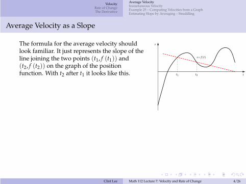
The formula for the average velocity shouldlook familiar. It just represents the slope of theline joining the two points (t1, f (t1)) and(t2, f (t2)) on the graph of the positionfunction. With t2 after t1 it looks like this. t
s
t1 t2
s= f (t)
Clint Lee Math 112 Lecture 7: Velocity and Rate of Change 4/26
VelocityRate of ChangeThe Derivative
Average VelocityInstantaneous VelocityExample 25 – Computing Velocities from a GraphEstimating Slope by Averaging – Straddling
Average Velocity as a Slope
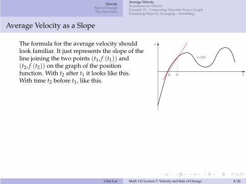
The formula for the average velocity shouldlook familiar. It just represents the slope of theline joining the two points (t1, f (t1)) and(t2, f (t2)) on the graph of the positionfunction. With t2 after t1 it looks like this.With time t2 before t1, like this.
t
s
t1t2
s= f (t)
Clint Lee Math 112 Lecture 7: Velocity and Rate of Change 4/26

VelocityRate of ChangeThe Derivative
Average VelocityInstantaneous VelocityExample 25 – Computing Velocities from a GraphEstimating Slope by Averaging – Straddling
Average Velocity as a Slope
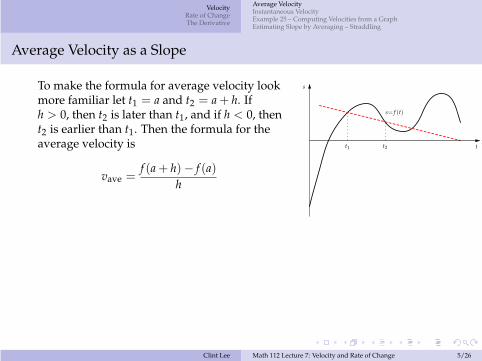
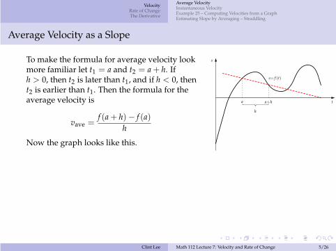
To make the formula for average velocity lookmore familiar let t1 = a and t2 = a + h. Ifh > 0, then t2 is later than t1, and if h < 0, thent2 is earlier than t1. Then the formula for theaverage velocity is t
s
t1 t2
s= f (t)
Clint Lee Math 112 Lecture 7: Velocity and Rate of Change 5/26
VelocityRate of ChangeThe Derivative
Average VelocityInstantaneous VelocityExample 25 – Computing Velocities from a GraphEstimating Slope by Averaging – Straddling
Average Velocity as a Slope
To make the formula for average velocity lookmore familiar let t1 = a and t2 = a + h. Ifh > 0, then t2 is later than t1, and if h < 0, thent2 is earlier than t1. Then the formula for theaverage velocity is
vave =f (a + h) − f (a)
h
t
s
t1 t2
s= f (t)
Clint Lee Math 112 Lecture 7: Velocity and Rate of Change 5/26
VelocityRate of ChangeThe Derivative
Average VelocityInstantaneous VelocityExample 25 – Computing Velocities from a GraphEstimating Slope by Averaging – Straddling
Average Velocity as a Slope
To make the formula for average velocity lookmore familiar let t1 = a and t2 = a + h. Ifh > 0, then t2 is later than t1, and if h < 0, thent2 is earlier than t1. Then the formula for theaverage velocity is
vave =f (a + h) − f (a)
h
Now the graph looks like this.
t
s
a a+h
h
s= f (t)
Clint Lee Math 112 Lecture 7: Velocity and Rate of Change 5/26
VelocityRate of ChangeThe Derivative
Average VelocityInstantaneous VelocityExample 25 – Computing Velocities from a GraphEstimating Slope by Averaging – Straddling
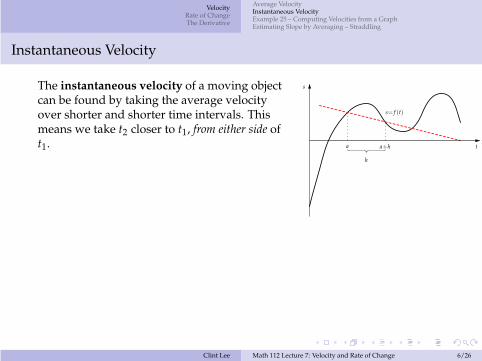
Instantaneous Velocity
The instantaneous velocity of a moving objectcan be found by taking the average velocityover shorter and shorter time intervals. Thismeans we take t2 closer to t1, from either side oft1. t
s
a a+h
h
s= f (t)
Clint Lee Math 112 Lecture 7: Velocity and Rate of Change 6/26
VelocityRate of ChangeThe Derivative
Average VelocityInstantaneous VelocityExample 25 – Computing Velocities from a GraphEstimating Slope by Averaging – Straddling
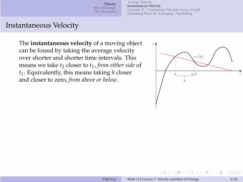
Instantaneous Velocity
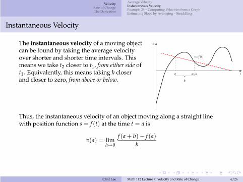
The instantaneous velocity of a moving objectcan be found by taking the average velocityover shorter and shorter time intervals. Thismeans we take t2 closer to t1, from either side oft1. Equivalently, this means taking h closerand closer to zero, from above or below.
t
s
a a+h
h
s= f (t)
Clint Lee Math 112 Lecture 7: Velocity and Rate of Change 6/26
VelocityRate of ChangeThe Derivative
Average VelocityInstantaneous VelocityExample 25 – Computing Velocities from a GraphEstimating Slope by Averaging – Straddling
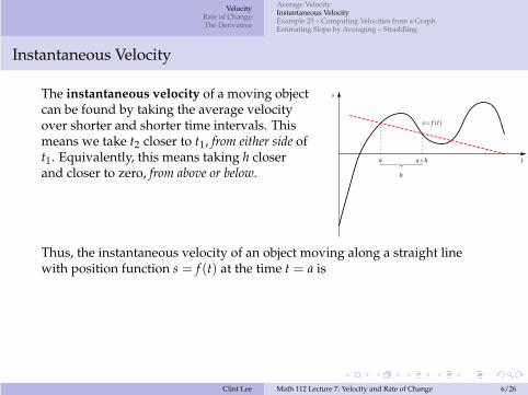
Instantaneous Velocity
The instantaneous velocity of a moving objectcan be found by taking the average velocityover shorter and shorter time intervals. Thismeans we take t2 closer to t1, from either side oft1. Equivalently, this means taking h closerand closer to zero, from above or below.
t
s
a a+h
h
s= f (t)
Thus, the instantaneous velocity of an object moving along a straight linewith position function s = f (t) at the time t = a is
Clint Lee Math 112 Lecture 7: Velocity and Rate of Change 6/26
VelocityRate of ChangeThe Derivative
Average VelocityInstantaneous VelocityExample 25 – Computing Velocities from a GraphEstimating Slope by Averaging – Straddling
Instantaneous Velocity
The instantaneous velocity of a moving objectcan be found by taking the average velocityover shorter and shorter time intervals. Thismeans we take t2 closer to t1, from either side oft1. Equivalently, this means taking h closerand closer to zero, from above or below.
t
s
a a+h
h
s= f (t)
Thus, the instantaneous velocity of an object moving along a straight linewith position function s = f (t) at the time t = a is
v(a) = limh→0
f (a + h) − f (a)h
Clint Lee Math 112 Lecture 7: Velocity and Rate of Change 6/26
VelocityRate of ChangeThe Derivative
Average VelocityInstantaneous VelocityExample 25 – Computing Velocities from a GraphEstimating Slope by Averaging – Straddling
Instantaneous Velocity
The instantaneous velocity of a moving objectcan be found by taking the average velocityover shorter and shorter time intervals. Thismeans we take t2 closer to t1, from either side oft1. Equivalently, this means taking h closerand closer to zero, from above or below.
t
s
a
s= f (t)
Thus, the instantaneous velocity of an object moving along a straight linewith position function s = f (t) at the time t = a is
v(a) = limh→0
f (a + h) − f (a)h
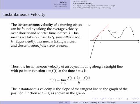
The instantaneous velocity is the slope of the tangent line to the graph of theposition function at t = a, as shown in the graph.
Clint Lee Math 112 Lecture 7: Velocity and Rate of Change 6/26
VelocityRate of ChangeThe Derivative
Average VelocityInstantaneous VelocityExample 25 – Computing Velocities from a GraphEstimating Slope by Averaging – Straddling
Example 25 – Computing Velocities from a Graph
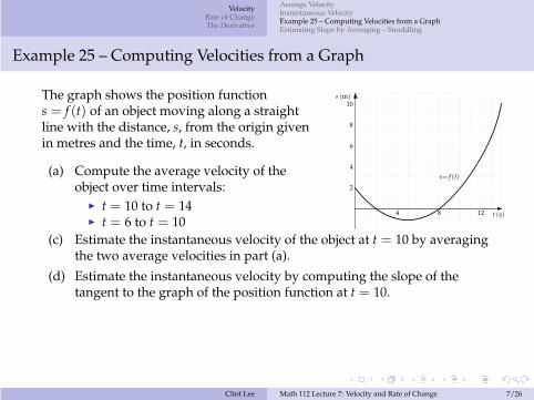
The graph shows the position functions = f (t) of an object moving along a straightline with the distance, s, from the origin givenin metres and the time, t, in seconds.
(a) Compute the average velocity of theobject over time intervals:
I t = 10 to t = 14I t = 6 to t = 10
2
4
6
8
10
4 8 12 t (s)
s (m)
s= f (t)
(c) Estimate the instantaneous velocity of the object at t = 10 by averagingthe two average velocities in part (a).
(d) Estimate the instantaneous velocity by computing the slope of thetangent to the graph of the position function at t = 10.
Clint Lee Math 112 Lecture 7: Velocity and Rate of Change 7/26
VelocityRate of ChangeThe Derivative
Average VelocityInstantaneous VelocityExample 25 – Computing Velocities from a GraphEstimating Slope by Averaging – Straddling
Solution: Example 25(a) & (b)
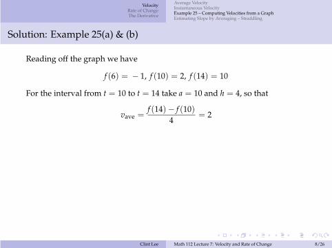
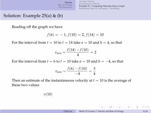
Reading off the graph we have
Clint Lee Math 112 Lecture 7: Velocity and Rate of Change 8/26
VelocityRate of ChangeThe Derivative
Average VelocityInstantaneous VelocityExample 25 – Computing Velocities from a GraphEstimating Slope by Averaging – Straddling
Solution: Example 25(a) & (b)
Reading off the graph we have
f (6) = − 1
Clint Lee Math 112 Lecture 7: Velocity and Rate of Change 8/26
VelocityRate of ChangeThe Derivative
Average VelocityInstantaneous VelocityExample 25 – Computing Velocities from a GraphEstimating Slope by Averaging – Straddling
Solution: Example 25(a) & (b)
Reading off the graph we have
f (6) = − 1, f (10) = 2
Clint Lee Math 112 Lecture 7: Velocity and Rate of Change 8/26
VelocityRate of ChangeThe Derivative
Average VelocityInstantaneous VelocityExample 25 – Computing Velocities from a GraphEstimating Slope by Averaging – Straddling
Solution: Example 25(a) & (b)
Reading off the graph we have
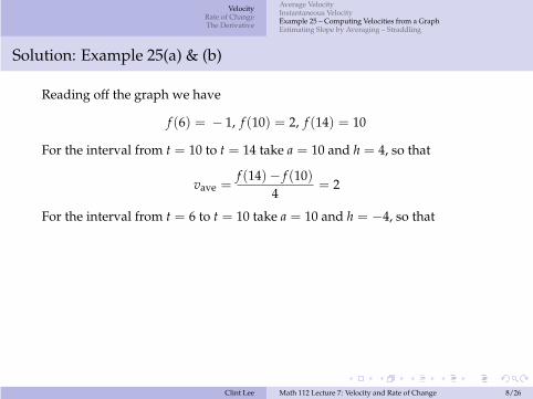
f (6) = − 1, f (10) = 2, f (14) = 10
Clint Lee Math 112 Lecture 7: Velocity and Rate of Change 8/26
VelocityRate of ChangeThe Derivative
Average VelocityInstantaneous VelocityExample 25 – Computing Velocities from a GraphEstimating Slope by Averaging – Straddling
Solution: Example 25(a) & (b)
Reading off the graph we have
f (6) = − 1, f (10) = 2, f (14) = 10
For the interval from t = 10 to t = 14 take a = 10 and h = 4, so that
vave =f (14) − f (10)
4= 2
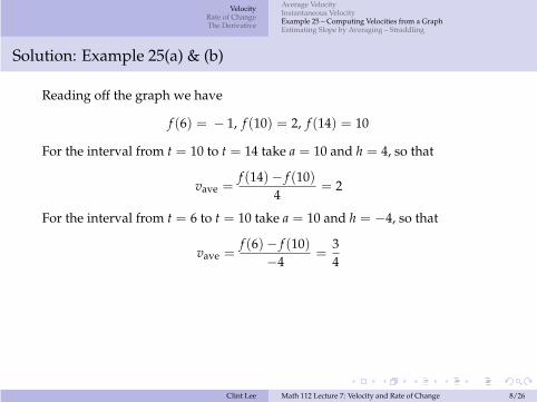
For the interval from t = 6 to t = 10 take a = 10 and h = −4, so that
Clint Lee Math 112 Lecture 7: Velocity and Rate of Change 8/26
VelocityRate of ChangeThe Derivative
Average VelocityInstantaneous VelocityExample 25 – Computing Velocities from a GraphEstimating Slope by Averaging – Straddling
Solution: Example 25(a) & (b)
Reading off the graph we have
f (6) = − 1, f (10) = 2, f (14) = 10
For the interval from t = 10 to t = 14 take a = 10 and h = 4, so that
vave =f (14) − f (10)
4= 2
For the interval from t = 6 to t = 10 take a = 10 and h = −4, so that
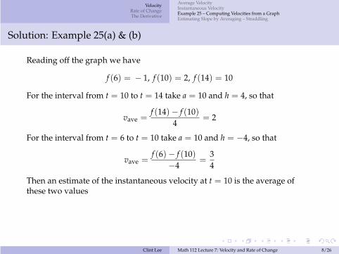
vave =f (6) − f (10)
−4=
34
Clint Lee Math 112 Lecture 7: Velocity and Rate of Change 8/26
VelocityRate of ChangeThe Derivative
Average VelocityInstantaneous VelocityExample 25 – Computing Velocities from a GraphEstimating Slope by Averaging – Straddling
Solution: Example 25(a) & (b)
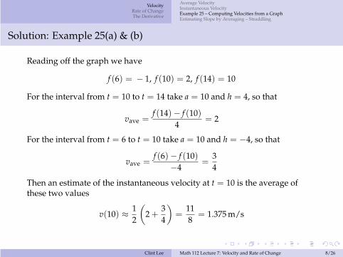
Reading off the graph we have
f (6) = − 1, f (10) = 2, f (14) = 10
For the interval from t = 10 to t = 14 take a = 10 and h = 4, so that
vave =f (14) − f (10)
4= 2
For the interval from t = 6 to t = 10 take a = 10 and h = −4, so that
vave =f (6) − f (10)
−4=
34
Then an estimate of the instantaneous velocity at t = 10 is the average ofthese two values
Clint Lee Math 112 Lecture 7: Velocity and Rate of Change 8/26
VelocityRate of ChangeThe Derivative
Average VelocityInstantaneous VelocityExample 25 – Computing Velocities from a GraphEstimating Slope by Averaging – Straddling
Solution: Example 25(a) & (b)
Reading off the graph we have
f (6) = − 1, f (10) = 2, f (14) = 10
For the interval from t = 10 to t = 14 take a = 10 and h = 4, so that
vave =f (14) − f (10)
4= 2
For the interval from t = 6 to t = 10 take a = 10 and h = −4, so that
vave =f (6) − f (10)
−4=
34
Then an estimate of the instantaneous velocity at t = 10 is the average ofthese two values
v(10)
Clint Lee Math 112 Lecture 7: Velocity and Rate of Change 8/26
VelocityRate of ChangeThe Derivative
Average VelocityInstantaneous VelocityExample 25 – Computing Velocities from a GraphEstimating Slope by Averaging – Straddling
Solution: Example 25(a) & (b)
Reading off the graph we have
f (6) = − 1, f (10) = 2, f (14) = 10
For the interval from t = 10 to t = 14 take a = 10 and h = 4, so that
vave =f (14) − f (10)
4= 2
For the interval from t = 6 to t = 10 take a = 10 and h = −4, so that
vave =f (6) − f (10)
−4=
34
Then an estimate of the instantaneous velocity at t = 10 is the average ofthese two values
v(10) ≈12
(
2 +34
)
=118
= 1.375 m/s
Clint Lee Math 112 Lecture 7: Velocity and Rate of Change 8/26
VelocityRate of ChangeThe Derivative
Average VelocityInstantaneous VelocityExample 25 – Computing Velocities from a GraphEstimating Slope by Averaging – Straddling
Solution: Example 25(c)
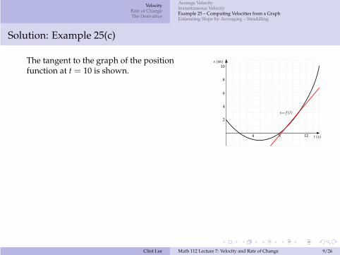
The tangent to the graph of the positionfunction at t = 10 is shown.
2
4
6
8
10
4 8 12 t (s)
s (m)
s= f (t)
Clint Lee Math 112 Lecture 7: Velocity and Rate of Change 9/26

VelocityRate of ChangeThe Derivative
Average VelocityInstantaneous VelocityExample 25 – Computing Velocities from a GraphEstimating Slope by Averaging – Straddling
Solution: Example 25(c)
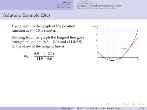
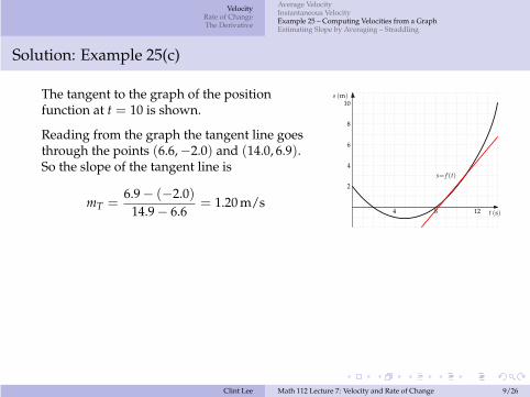
The tangent to the graph of the positionfunction at t = 10 is shown.
Reading from the graph the tangent line goesthrough the points (6.6,−2.0) and (14.0, 6.9).
2
4
6
8
10
4 8 12 t (s)
s (m)
s= f (t)
Clint Lee Math 112 Lecture 7: Velocity and Rate of Change 9/26
VelocityRate of ChangeThe Derivative
Average VelocityInstantaneous VelocityExample 25 – Computing Velocities from a GraphEstimating Slope by Averaging – Straddling
Solution: Example 25(c)
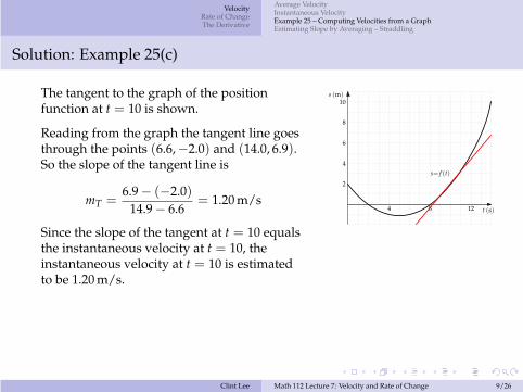
The tangent to the graph of the positionfunction at t = 10 is shown.
Reading from the graph the tangent line goesthrough the points (6.6,−2.0) and (14.0, 6.9).So the slope of the tangent line is
mT =6.9 − (−2.0)
14.9 − 6.6
2
4
6
8
10
4 8 12 t (s)
s (m)
s= f (t)
Clint Lee Math 112 Lecture 7: Velocity and Rate of Change 9/26
VelocityRate of ChangeThe Derivative
Average VelocityInstantaneous VelocityExample 25 – Computing Velocities from a GraphEstimating Slope by Averaging – Straddling
Solution: Example 25(c)
The tangent to the graph of the positionfunction at t = 10 is shown.
Reading from the graph the tangent line goesthrough the points (6.6,−2.0) and (14.0, 6.9).So the slope of the tangent line is
mT =6.9 − (−2.0)
14.9 − 6.6= 1.20 m/s
Since the slope of the tangent at t = 10 equalsthe instantaneous velocity at t = 10, theinstantaneous velocity at t = 10 is estimatedto be 1.20 m/s.
2
4
6
8
10
4 8 12 t (s)
s (m)
s= f (t)
Clint Lee Math 112 Lecture 7: Velocity and Rate of Change 9/26
VelocityRate of ChangeThe Derivative
Average VelocityInstantaneous VelocityExample 25 – Computing Velocities from a GraphEstimating Slope by Averaging – Straddling
Estimating Slope by Averaging – Straddling
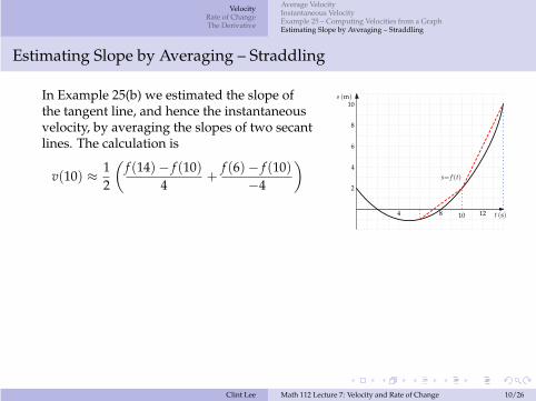
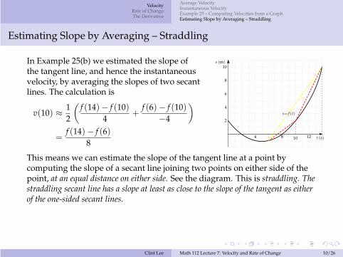
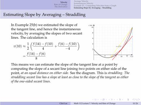
In Example 25(b) we estimated the slope ofthe tangent line, and hence the instantaneousvelocity, by averaging the slopes of two secantlines. The calculation is
v(10) ≈12
(
f (14) − f (10)
4+
f (6) − f (10)
−4
)
2
4
6
8
10
4 8 12 t (s)
s (m)
10
s= f (t)
Clint Lee Math 112 Lecture 7: Velocity and Rate of Change 10/26

VelocityRate of ChangeThe Derivative
Average VelocityInstantaneous VelocityExample 25 – Computing Velocities from a GraphEstimating Slope by Averaging – Straddling
Estimating Slope by Averaging – Straddling
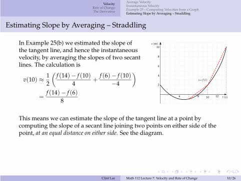
In Example 25(b) we estimated the slope ofthe tangent line, and hence the instantaneousvelocity, by averaging the slopes of two secantlines. The calculation is
v(10) ≈12
(
f (14) − f (10)
4+
f (6) − f (10)
−4
)
=f (14) − f (6)
8
2
4
6
8
10
4 8 12 t (s)
s (m)
10
s= f (t)
Clint Lee Math 112 Lecture 7: Velocity and Rate of Change 10/26
VelocityRate of ChangeThe Derivative
Average VelocityInstantaneous VelocityExample 25 – Computing Velocities from a GraphEstimating Slope by Averaging – Straddling
Estimating Slope by Averaging – Straddling
In Example 25(b) we estimated the slope ofthe tangent line, and hence the instantaneousvelocity, by averaging the slopes of two secantlines. The calculation is
v(10) ≈12
(
f (14) − f (10)
4+
f (6) − f (10)
−4
)
=f (14) − f (6)
8
2
4
6
8
10
4 8 12 t (s)
s (m)
10
s= f (t)
This means we can estimate the slope of the tangent line at a point bycomputing the slope of a secant line joining two points on either side of thepoint, at an equal distance on either side. See the diagram.
Clint Lee Math 112 Lecture 7: Velocity and Rate of Change 10/26
VelocityRate of ChangeThe Derivative
Average VelocityInstantaneous VelocityExample 25 – Computing Velocities from a GraphEstimating Slope by Averaging – Straddling
Estimating Slope by Averaging – Straddling
In Example 25(b) we estimated the slope ofthe tangent line, and hence the instantaneousvelocity, by averaging the slopes of two secantlines. The calculation is
v(10) ≈12
(
f (14) − f (10)
4+
f (6) − f (10)
−4
)
=f (14) − f (6)
8
2
4
6
8
10
4 8 12 t (s)
s (m)
10
s= f (t)
This means we can estimate the slope of the tangent line at a point bycomputing the slope of a secant line joining two points on either side of thepoint, at an equal distance on either side. See the diagram. This is straddling. Thestraddling secant line has a slope at least as close to the slope of the tangent as eitherof the one-sided secant lines.
Clint Lee Math 112 Lecture 7: Velocity and Rate of Change 10/26
VelocityRate of ChangeThe Derivative
Average Rate of ChangeInstantaneous Rate of ChangeExample 26 – Rate of Change of Area
Increments and Average Rate of Change
Suppose that quantity y is a function of another quantity x, y = f (x).
Clint Lee Math 112 Lecture 7: Velocity and Rate of Change 11/26
VelocityRate of ChangeThe Derivative
Average Rate of ChangeInstantaneous Rate of ChangeExample 26 – Rate of Change of Area
Increments and Average Rate of Change
Suppose that quantity y is a function of another quantity x, y = f (x). If xchanges from x1 to x2, the increment in x is
∆x = x2 − x1
and y changes from f (x1) to f (x2) for an increment of
∆y = f (x2) − f (x1)
The average rate of change of y with respect to x when x changes from x1 tox2 is
average rate of change =f (x2) − f (x1)
x2 − x1
Clint Lee Math 112 Lecture 7: Velocity and Rate of Change 11/26
VelocityRate of ChangeThe Derivative
Average Rate of ChangeInstantaneous Rate of ChangeExample 26 – Rate of Change of Area
Increments and Average Rate of Change
Suppose that quantity y is a function of another quantity x, y = f (x). If xchanges from x1 to x2, the increment in x is
∆x = x2 − x1
and y changes from f (x1) to f (x2) for an increment of
∆y = f (x2) − f (x1)
The average rate of change of y with respect to x when x changes from x1 tox2 is
average rate of change =f (x2) − f (x1)
x2 − x1=
∆y∆x
This rate of change can also be described as the change in y per unit change inx.
Clint Lee Math 112 Lecture 7: Velocity and Rate of Change 11/26
VelocityRate of ChangeThe Derivative
Average Rate of ChangeInstantaneous Rate of ChangeExample 26 – Rate of Change of Area
Slope and Velocity as Rates of Change
The slope of a line is the rate of change of the y-coordinate of points on theline with respect to the x-coordinate.
The velocity of a moving object is the rate of change of the position of theobject with respect to time.
Clint Lee Math 112 Lecture 7: Velocity and Rate of Change 12/26
VelocityRate of ChangeThe Derivative
Average Rate of ChangeInstantaneous Rate of ChangeExample 26 – Rate of Change of Area
Instantaneous Rate of Change
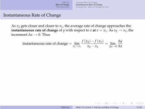
As x2 gets closer and closer to x1, the average rate of change approaches theinstantaneous rate of change of y with respect to x at x = x1.
Clint Lee Math 112 Lecture 7: Velocity and Rate of Change 13/26
VelocityRate of ChangeThe Derivative
Average Rate of ChangeInstantaneous Rate of ChangeExample 26 – Rate of Change of Area
Instantaneous Rate of Change
As x2 gets closer and closer to x1, the average rate of change approaches theinstantaneous rate of change of y with respect to x at x = x1. As x2 → x1, theincrement ∆x → 0. Thus
instantaneous rate of change
Clint Lee Math 112 Lecture 7: Velocity and Rate of Change 13/26
VelocityRate of ChangeThe Derivative
Average Rate of ChangeInstantaneous Rate of ChangeExample 26 – Rate of Change of Area
Instantaneous Rate of Change
As x2 gets closer and closer to x1, the average rate of change approaches theinstantaneous rate of change of y with respect to x at x = x1. As x2 → x1, theincrement ∆x → 0. Thus
instantaneous rate of change = limx2→x1
f (x2) − f (x1)
x2 − x1
Clint Lee Math 112 Lecture 7: Velocity and Rate of Change 13/26
VelocityRate of ChangeThe Derivative
Average Rate of ChangeInstantaneous Rate of ChangeExample 26 – Rate of Change of Area
Instantaneous Rate of Change
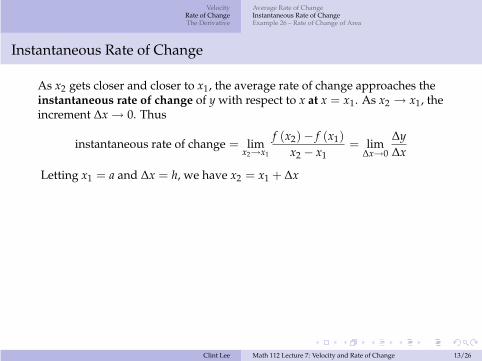
As x2 gets closer and closer to x1, the average rate of change approaches theinstantaneous rate of change of y with respect to x at x = x1. As x2 → x1, theincrement ∆x → 0. Thus
instantaneous rate of change = limx2→x1
f (x2) − f (x1)
x2 − x1= lim
∆x→0
∆y∆x
Clint Lee Math 112 Lecture 7: Velocity and Rate of Change 13/26
VelocityRate of ChangeThe Derivative
Average Rate of ChangeInstantaneous Rate of ChangeExample 26 – Rate of Change of Area
Instantaneous Rate of Change
As x2 gets closer and closer to x1, the average rate of change approaches theinstantaneous rate of change of y with respect to x at x = x1. As x2 → x1, theincrement ∆x → 0. Thus
instantaneous rate of change = limx2→x1
f (x2) − f (x1)
x2 − x1= lim
∆x→0
∆y∆x
Letting x1 = a and ∆x = h, we have x2 = x1 + ∆x
Clint Lee Math 112 Lecture 7: Velocity and Rate of Change 13/26
VelocityRate of ChangeThe Derivative
Average Rate of ChangeInstantaneous Rate of ChangeExample 26 – Rate of Change of Area
Instantaneous Rate of Change
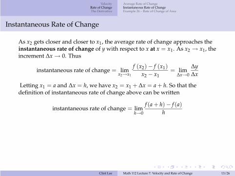
As x2 gets closer and closer to x1, the average rate of change approaches theinstantaneous rate of change of y with respect to x at x = x1. As x2 → x1, theincrement ∆x → 0. Thus
instantaneous rate of change = limx2→x1
f (x2) − f (x1)
x2 − x1= lim
∆x→0
∆y∆x
Letting x1 = a and ∆x = h, we have x2 = x1 + ∆x = a + h. So that thedefinition of instantaneous rate of change above can be written
instantaneous rate of change = limh→0
f (a + h) − f (a)h
Clint Lee Math 112 Lecture 7: Velocity and Rate of Change 13/26
VelocityRate of ChangeThe Derivative
Average Rate of ChangeInstantaneous Rate of ChangeExample 26 – Rate of Change of Area
Example 26 – Rate of Change of Area
The area A of a square with side length s is A = f (s) = s2.
(a) Determine the average rate of change of the area of a square when theside length changes from
I s = 5 m to s = 6 mI s = 5 m to s = 5.5 mI s = 5 m to s = 5.1 m
Give the units of the rate of change.
(b) Determine the instantaneous rate of change of the area of the squarewith respect to its side length when the side length is s = 5 m.
Clint Lee Math 112 Lecture 7: Velocity and Rate of Change 14/26
VelocityRate of ChangeThe Derivative
Average Rate of ChangeInstantaneous Rate of ChangeExample 26 – Rate of Change of Area
Solution: Example 26(a)
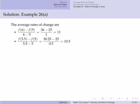
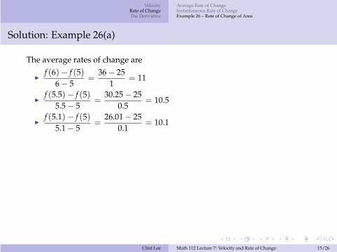
The average rates of change are
Clint Lee Math 112 Lecture 7: Velocity and Rate of Change 15/26

VelocityRate of ChangeThe Derivative
Average Rate of ChangeInstantaneous Rate of ChangeExample 26 – Rate of Change of Area
Solution: Example 26(a)
The average rates of change are
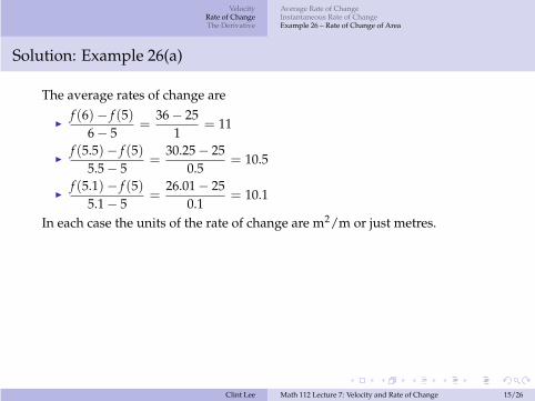
I
f (6) − f (5)
6 − 5=
36 − 251
= 11
Clint Lee Math 112 Lecture 7: Velocity and Rate of Change 15/26
VelocityRate of ChangeThe Derivative
Average Rate of ChangeInstantaneous Rate of ChangeExample 26 – Rate of Change of Area
Solution: Example 26(a)
The average rates of change are
I
f (6) − f (5)
6 − 5=
36 − 251
= 11
I
f (5.5) − f (5)
5.5 − 5=
30.25 − 250.5
= 10.5
I
f (5.1) − f (5)
5.1 − 5=
26.01 − 250.1
= 10.1
In each case the units of the rate of change are m2/m or just metres.
Clint Lee Math 112 Lecture 7: Velocity and Rate of Change 15/26
VelocityRate of ChangeThe Derivative
Average Rate of ChangeInstantaneous Rate of ChangeExample 26 – Rate of Change of Area
Solution: Example 26(b)
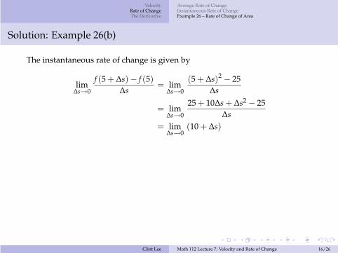
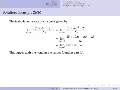
The instantaneous rate of change is given by
Clint Lee Math 112 Lecture 7: Velocity and Rate of Change 16/26
VelocityRate of ChangeThe Derivative
Average Rate of ChangeInstantaneous Rate of ChangeExample 26 – Rate of Change of Area
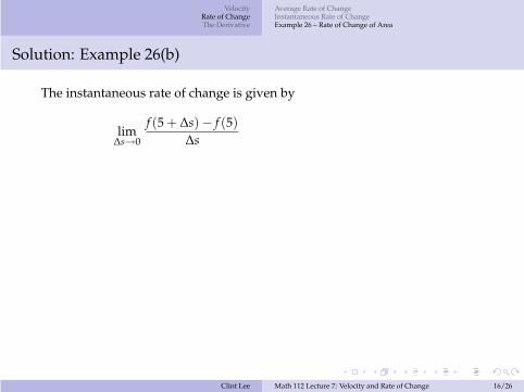
Solution: Example 26(b)
The instantaneous rate of change is given by
lim∆s→0
f (5 + ∆s) − f (5)
∆s
Clint Lee Math 112 Lecture 7: Velocity and Rate of Change 16/26
VelocityRate of ChangeThe Derivative
Average Rate of ChangeInstantaneous Rate of ChangeExample 26 – Rate of Change of Area
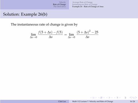
Solution: Example 26(b)
The instantaneous rate of change is given by
lim∆s→0
f (5 + ∆s) − f (5)
∆s= lim
∆s→0
(5 + ∆s)2− 25
∆s
Clint Lee Math 112 Lecture 7: Velocity and Rate of Change 16/26
VelocityRate of ChangeThe Derivative
Average Rate of ChangeInstantaneous Rate of ChangeExample 26 – Rate of Change of Area
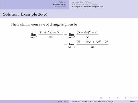
Solution: Example 26(b)
The instantaneous rate of change is given by
lim∆s→0
f (5 + ∆s) − f (5)
∆s= lim
∆s→0
(5 + ∆s)2− 25
∆s
= lim∆s→0
25 + 10∆s + ∆s2− 25
∆s
Clint Lee Math 112 Lecture 7: Velocity and Rate of Change 16/26
VelocityRate of ChangeThe Derivative
Average Rate of ChangeInstantaneous Rate of ChangeExample 26 – Rate of Change of Area
Solution: Example 26(b)
The instantaneous rate of change is given by
lim∆s→0
f (5 + ∆s) − f (5)
∆s= lim
∆s→0
(5 + ∆s)2− 25
∆s
= lim∆s→0
25 + 10∆s + ∆s2− 25
∆s= lim
∆s→0(10 + ∆s)
Clint Lee Math 112 Lecture 7: Velocity and Rate of Change 16/26

VelocityRate of ChangeThe Derivative
Average Rate of ChangeInstantaneous Rate of ChangeExample 26 – Rate of Change of Area
Solution: Example 26(b)
The instantaneous rate of change is given by
lim∆s→0
f (5 + ∆s) − f (5)
∆s= lim
∆s→0
(5 + ∆s)2− 25
∆s
= lim∆s→0
25 + 10∆s + ∆s2− 25
∆s= lim
∆s→0(10 + ∆s) = 10
Clint Lee Math 112 Lecture 7: Velocity and Rate of Change 16/26
VelocityRate of ChangeThe Derivative
Average Rate of ChangeInstantaneous Rate of ChangeExample 26 – Rate of Change of Area
Solution: Example 26(b)
The instantaneous rate of change is given by
lim∆s→0
f (5 + ∆s) − f (5)
∆s= lim
∆s→0
(5 + ∆s)2− 25
∆s
= lim∆s→0
25 + 10∆s + ∆s2− 25
∆s= lim
∆s→0(10 + ∆s) = 10
This agrees with the trend in the values found in part (a).
Clint Lee Math 112 Lecture 7: Velocity and Rate of Change 16/26
VelocityRate of ChangeThe Derivative
Average Rate of ChangeInstantaneous Rate of ChangeExample 26 – Rate of Change of Area
Solution: Example 26 Comment
Consider the change in the area of the squarewhen the side length increases from s = 5 m tos = 6 m. This is shown in the diagram, wherethe the shaded portions represent the change inarea.
Clint Lee Math 112 Lecture 7: Velocity and Rate of Change 17/26
VelocityRate of ChangeThe Derivative
Average Rate of ChangeInstantaneous Rate of ChangeExample 26 – Rate of Change of Area
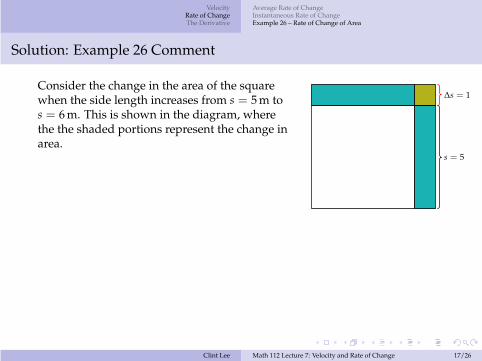
Solution: Example 26 Comment
Consider the change in the area of the squarewhen the side length increases from s = 5 m tos = 6 m. This is shown in the diagram, wherethe the shaded portions represent the change inarea.
s = 5
∆s = 1
Clint Lee Math 112 Lecture 7: Velocity and Rate of Change 17/26
VelocityRate of ChangeThe Derivative
Average Rate of ChangeInstantaneous Rate of ChangeExample 26 – Rate of Change of Area
Solution: Example 26 Comment
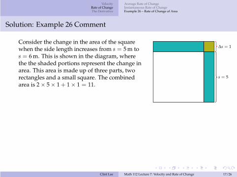
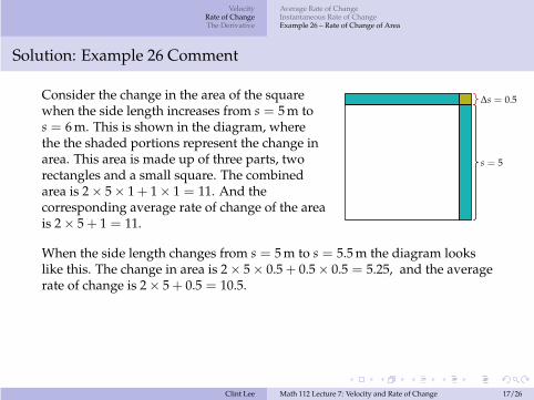
Consider the change in the area of the squarewhen the side length increases from s = 5 m tos = 6 m. This is shown in the diagram, wherethe the shaded portions represent the change inarea. This area is made up of three parts, tworectangles and a small square. The combinedarea is 2 × 5 × 1 + 1 × 1 = 11.
s = 5
∆s = 1
Clint Lee Math 112 Lecture 7: Velocity and Rate of Change 17/26
VelocityRate of ChangeThe Derivative
Average Rate of ChangeInstantaneous Rate of ChangeExample 26 – Rate of Change of Area
Solution: Example 26 Comment
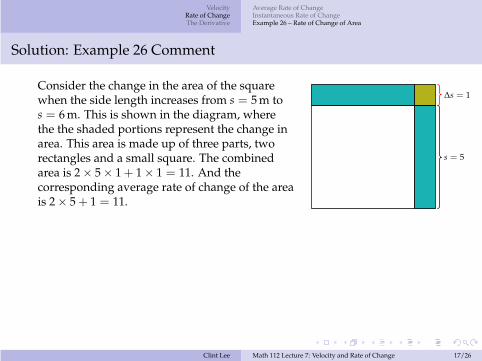
Consider the change in the area of the squarewhen the side length increases from s = 5 m tos = 6 m. This is shown in the diagram, wherethe the shaded portions represent the change inarea. This area is made up of three parts, tworectangles and a small square. The combinedarea is 2 × 5 × 1 + 1 × 1 = 11. And thecorresponding average rate of change of the areais 2 × 5 + 1 = 11.
s = 5
∆s = 1
Clint Lee Math 112 Lecture 7: Velocity and Rate of Change 17/26
VelocityRate of ChangeThe Derivative
Average Rate of ChangeInstantaneous Rate of ChangeExample 26 – Rate of Change of Area
Solution: Example 26 Comment
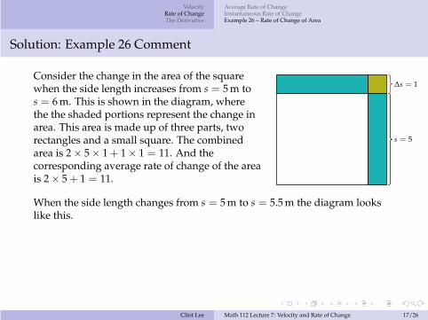
Consider the change in the area of the squarewhen the side length increases from s = 5 m tos = 6 m. This is shown in the diagram, wherethe the shaded portions represent the change inarea. This area is made up of three parts, tworectangles and a small square. The combinedarea is 2 × 5 × 1 + 1 × 1 = 11. And thecorresponding average rate of change of the areais 2 × 5 + 1 = 11.
s = 5
∆s = 1
When the side length changes from s = 5 m to s = 5.5 m the diagram lookslike this.
Clint Lee Math 112 Lecture 7: Velocity and Rate of Change 17/26
VelocityRate of ChangeThe Derivative
Average Rate of ChangeInstantaneous Rate of ChangeExample 26 – Rate of Change of Area
Solution: Example 26 Comment
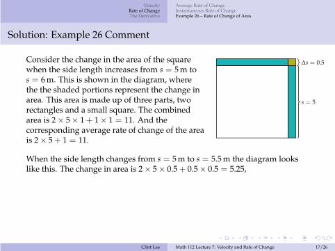
Consider the change in the area of the squarewhen the side length increases from s = 5 m tos = 6 m. This is shown in the diagram, wherethe the shaded portions represent the change inarea. This area is made up of three parts, tworectangles and a small square. The combinedarea is 2 × 5 × 1 + 1 × 1 = 11. And thecorresponding average rate of change of the areais 2 × 5 + 1 = 11.
s = 5
∆s = 0.5
When the side length changes from s = 5 m to s = 5.5 m the diagram lookslike this. The change in area is 2 × 5 × 0.5 + 0.5 × 0.5 = 5.25,
Clint Lee Math 112 Lecture 7: Velocity and Rate of Change 17/26
VelocityRate of ChangeThe Derivative
Average Rate of ChangeInstantaneous Rate of ChangeExample 26 – Rate of Change of Area
Solution: Example 26 Comment
Consider the change in the area of the squarewhen the side length increases from s = 5 m tos = 6 m. This is shown in the diagram, wherethe the shaded portions represent the change inarea. This area is made up of three parts, tworectangles and a small square. The combinedarea is 2 × 5 × 1 + 1 × 1 = 11. And thecorresponding average rate of change of the areais 2 × 5 + 1 = 11.
s = 5
∆s = 0.5
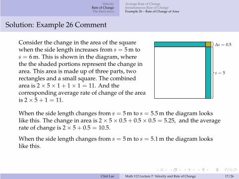
When the side length changes from s = 5 m to s = 5.5 m the diagram lookslike this. The change in area is 2 × 5 × 0.5 + 0.5 × 0.5 = 5.25, and the averagerate of change is 2 × 5 + 0.5 = 10.5.
Clint Lee Math 112 Lecture 7: Velocity and Rate of Change 17/26
VelocityRate of ChangeThe Derivative
Average Rate of ChangeInstantaneous Rate of ChangeExample 26 – Rate of Change of Area
Solution: Example 26 Comment
Consider the change in the area of the squarewhen the side length increases from s = 5 m tos = 6 m. This is shown in the diagram, wherethe the shaded portions represent the change inarea. This area is made up of three parts, tworectangles and a small square. The combinedarea is 2 × 5 × 1 + 1 × 1 = 11. And thecorresponding average rate of change of the areais 2 × 5 + 1 = 11.
s = 5
∆s = 0.5
When the side length changes from s = 5 m to s = 5.5 m the diagram lookslike this. The change in area is 2 × 5 × 0.5 + 0.5 × 0.5 = 5.25, and the averagerate of change is 2 × 5 + 0.5 = 10.5.
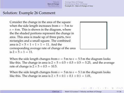
When the side length changes from s = 5 m to s = 5.1 m the diagram lookslike this.
Clint Lee Math 112 Lecture 7: Velocity and Rate of Change 17/26
VelocityRate of ChangeThe Derivative
Average Rate of ChangeInstantaneous Rate of ChangeExample 26 – Rate of Change of Area
Solution: Example 26 Comment
Consider the change in the area of the squarewhen the side length increases from s = 5 m tos = 6 m. This is shown in the diagram, wherethe the shaded portions represent the change inarea. This area is made up of three parts, tworectangles and a small square. The combinedarea is 2 × 5 × 1 + 1 × 1 = 11. And thecorresponding average rate of change of the areais 2 × 5 + 1 = 11.
When the side length changes from s = 5 m to s = 5.5 m the diagram lookslike this. The change in area is 2 × 5 × 0.5 + 0.5 × 0.5 = 5.25, and the averagerate of change is 2 × 5 + 0.5 = 10.5.
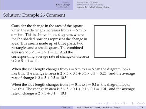
When the side length changes from s = 5 m to s = 5.1 m the diagram lookslike this. The change in area is 2 × 5 × 0.1 + 0.1 × 0.1 = 1.01,
Clint Lee Math 112 Lecture 7: Velocity and Rate of Change 17/26
VelocityRate of ChangeThe Derivative
Average Rate of ChangeInstantaneous Rate of ChangeExample 26 – Rate of Change of Area
Solution: Example 26 Comment
Consider the change in the area of the squarewhen the side length increases from s = 5 m tos = 6 m. This is shown in the diagram, wherethe the shaded portions represent the change inarea. This area is made up of three parts, tworectangles and a small square. The combinedarea is 2 × 5 × 1 + 1 × 1 = 11. And thecorresponding average rate of change of the areais 2 × 5 + 1 = 11.
When the side length changes from s = 5 m to s = 5.5 m the diagram lookslike this. The change in area is 2 × 5 × 0.5 + 0.5 × 0.5 = 5.25, and the averagerate of change is 2 × 5 + 0.5 = 10.5.
When the side length changes from s = 5 m to s = 5.1 m the diagram lookslike this. The change in area is 2 × 5 × 0.1 + 0.1 × 0.1 = 1.01, and the averagerate of change is 2 × 5 + 0.1 = 10.1.
Clint Lee Math 112 Lecture 7: Velocity and Rate of Change 17/26
VelocityRate of ChangeThe Derivative
Average Rate of ChangeInstantaneous Rate of ChangeExample 26 – Rate of Change of Area
Solution: Example 26 Comment continued
In general, the average rate of change of the area of the square when the sidelength changes from s = 5 to s = 5 + ∆s is
Clint Lee Math 112 Lecture 7: Velocity and Rate of Change 18/26
VelocityRate of ChangeThe Derivative
Average Rate of ChangeInstantaneous Rate of ChangeExample 26 – Rate of Change of Area
Solution: Example 26 Comment continued
In general, the average rate of change of the area of the square when the sidelength changes from s = 5 to s = 5 + ∆s is
average rate of change of area = 2 × 5 + ∆s
Clint Lee Math 112 Lecture 7: Velocity and Rate of Change 18/26
VelocityRate of ChangeThe Derivative
Average Rate of ChangeInstantaneous Rate of ChangeExample 26 – Rate of Change of Area
Solution: Example 26 Comment continued
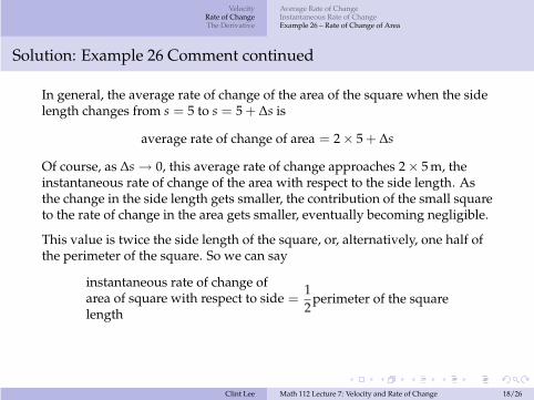
In general, the average rate of change of the area of the square when the sidelength changes from s = 5 to s = 5 + ∆s is
average rate of change of area = 2 × 5 + ∆s
Of course, as ∆s → 0, this average rate of change approaches 2 × 5 m, theinstantaneous rate of change of the area with respect to the side length. Asthe change in the side length gets smaller, the contribution of the small squareto the rate of change in the area gets smaller, eventually becoming negligible.
Clint Lee Math 112 Lecture 7: Velocity and Rate of Change 18/26
VelocityRate of ChangeThe Derivative
Average Rate of ChangeInstantaneous Rate of ChangeExample 26 – Rate of Change of Area
Solution: Example 26 Comment continued
In general, the average rate of change of the area of the square when the sidelength changes from s = 5 to s = 5 + ∆s is
average rate of change of area = 2 × 5 + ∆s
Of course, as ∆s → 0, this average rate of change approaches 2 × 5 m, theinstantaneous rate of change of the area with respect to the side length. Asthe change in the side length gets smaller, the contribution of the small squareto the rate of change in the area gets smaller, eventually becoming negligible.
This value is twice the side length of the square, or, alternatively, one half ofthe perimeter of the square. So we can say
instantaneous rate of change ofarea of square with respect to sidelength
=12
perimeter of the square
Clint Lee Math 112 Lecture 7: Velocity and Rate of Change 18/26
VelocityRate of ChangeThe Derivative
Average Rate of ChangeInstantaneous Rate of ChangeExample 26 – Rate of Change of Area
Solution: Example 26 Comment continued
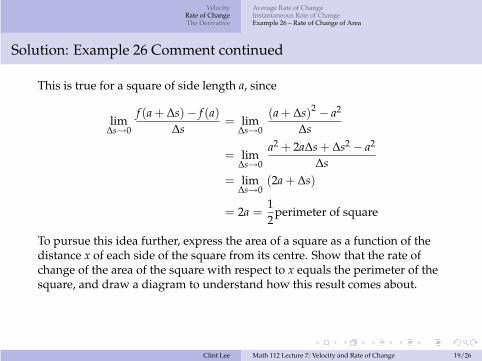
This is true for a square of side length a, since
Clint Lee Math 112 Lecture 7: Velocity and Rate of Change 19/26
VelocityRate of ChangeThe Derivative
Average Rate of ChangeInstantaneous Rate of ChangeExample 26 – Rate of Change of Area
Solution: Example 26 Comment continued
This is true for a square of side length a, since
lim∆s→0
f (a + ∆s) − f (a)∆s
= lim∆s→0
(a + ∆s)2− a2
∆s
= lim∆s→0
a2 + 2a∆s + ∆s2− a2
∆s
Clint Lee Math 112 Lecture 7: Velocity and Rate of Change 19/26
VelocityRate of ChangeThe Derivative
Average Rate of ChangeInstantaneous Rate of ChangeExample 26 – Rate of Change of Area
Solution: Example 26 Comment continued
This is true for a square of side length a, since
lim∆s→0
f (a + ∆s) − f (a)∆s
= lim∆s→0
(a + ∆s)2− a2
∆s
= lim∆s→0
a2 + 2a∆s + ∆s2− a2
∆s= lim
∆s→0(2a + ∆s)
= 2a
Clint Lee Math 112 Lecture 7: Velocity and Rate of Change 19/26
VelocityRate of ChangeThe Derivative
Average Rate of ChangeInstantaneous Rate of ChangeExample 26 – Rate of Change of Area
Solution: Example 26 Comment continued
This is true for a square of side length a, since
lim∆s→0
f (a + ∆s) − f (a)∆s
= lim∆s→0
(a + ∆s)2− a2
∆s
= lim∆s→0
a2 + 2a∆s + ∆s2− a2
∆s= lim
∆s→0(2a + ∆s)
= 2a =12
perimeter of square
To pursue this idea further, express the area of a square as a function of thedistance x of each side of the square from its centre. Show that the rate ofchange of the area of the square with respect to x equals the perimeter of thesquare, and draw a diagram to understand how this result comes about.
Clint Lee Math 112 Lecture 7: Velocity and Rate of Change 19/26

VelocityRate of ChangeThe Derivative
The Derivative at a PointExamples of DerivativesExample 27 – Calculating a Derivative at a Point
The Derivative at a Point
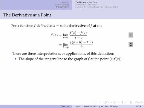
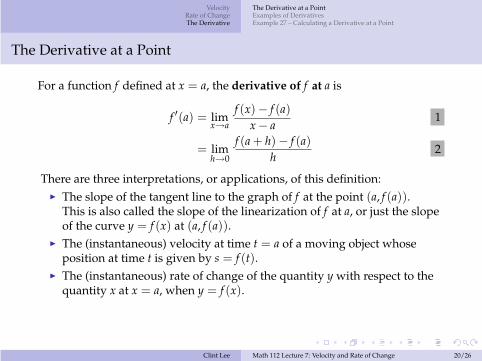
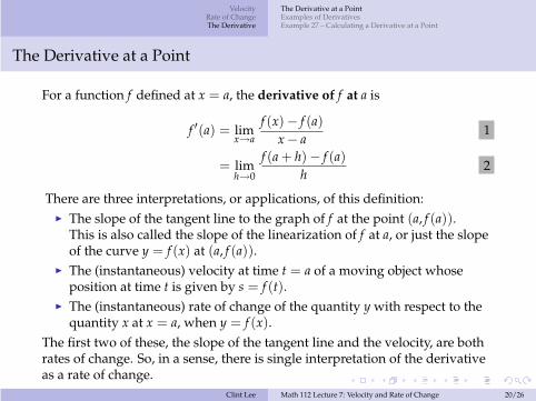
For a function f defined at x = a, the derivative of f at a is
f ′(a) = limx→a
f (x) − f (a)x − a
1
= limh→0
f (a + h) − f (a)h
2
Clint Lee Math 112 Lecture 7: Velocity and Rate of Change 20/26
VelocityRate of ChangeThe Derivative
The Derivative at a PointExamples of DerivativesExample 27 – Calculating a Derivative at a Point
The Derivative at a Point
For a function f defined at x = a, the derivative of f at a is
f ′(a) = limx→a
f (x) − f (a)x − a
1
= limh→0
f (a + h) − f (a)h
2
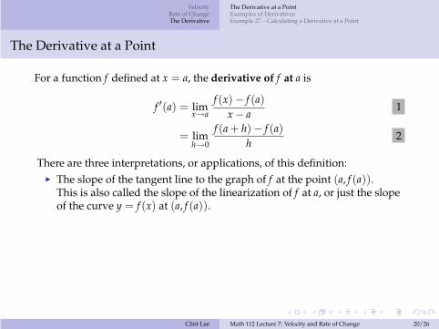
There are three interpretations, or applications, of this definition:I The slope of the tangent line to the graph of f at the point (a, f (a)).
Clint Lee Math 112 Lecture 7: Velocity and Rate of Change 20/26
VelocityRate of ChangeThe Derivative
The Derivative at a PointExamples of DerivativesExample 27 – Calculating a Derivative at a Point
The Derivative at a Point
For a function f defined at x = a, the derivative of f at a is
f ′(a) = limx→a
f (x) − f (a)x − a
1
= limh→0
f (a + h) − f (a)h
2
There are three interpretations, or applications, of this definition:I The slope of the tangent line to the graph of f at the point (a, f (a)).
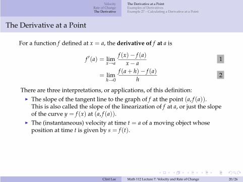
This is also called the slope of the linearization of f at a, or just the slopeof the curve y = f (x) at (a, f (a)).
Clint Lee Math 112 Lecture 7: Velocity and Rate of Change 20/26
VelocityRate of ChangeThe Derivative
The Derivative at a PointExamples of DerivativesExample 27 – Calculating a Derivative at a Point
The Derivative at a Point
For a function f defined at x = a, the derivative of f at a is
f ′(a) = limx→a
f (x) − f (a)x − a
1
= limh→0
f (a + h) − f (a)h
2
There are three interpretations, or applications, of this definition:I The slope of the tangent line to the graph of f at the point (a, f (a)).
This is also called the slope of the linearization of f at a, or just the slopeof the curve y = f (x) at (a, f (a)).
I The (instantaneous) velocity at time t = a of a moving object whoseposition at time t is given by s = f (t).
I The (instantaneous) rate of change of the quantity y with respect to thequantity x at x = a, when y = f (x).
The first two of these, the slope of the tangent line and the velocity, are bothrates of change. So, in a sense, there is single interpretation of the derivativeas a rate of change.
Clint Lee Math 112 Lecture 7: Velocity and Rate of Change 20/26
VelocityRate of ChangeThe Derivative
The Derivative at a PointExamples of DerivativesExample 27 – Calculating a Derivative at a Point
Examples of Derivatives
We have already computed or estimated derivatives.
Clint Lee Math 112 Lecture 7: Velocity and Rate of Change 21/26
VelocityRate of ChangeThe Derivative
The Derivative at a PointExamples of DerivativesExample 27 – Calculating a Derivative at a Point
Examples of Derivatives
We have already computed or estimated derivatives.
In Example 22 for the function f (x) = x3 we found that f ′(1) = 3. In thisexample the derivative gave us the slope, and so the equation of the linetangent to y = x3 at the point (1, 1).
In Example 25 we estimated f ′(10) to give the instantaneous velocity of amoving object whose position is given by s = f (t). The estimate was basedon the graph of the function f .
In Example 26 for the function A = f (s) = s2 we found that f ′(5) = 10, and,more generally, that f ′(a) = 2a. In this example the derivative gave us therate of change of the area A of a square with respect to its side length s.
Clint Lee Math 112 Lecture 7: Velocity and Rate of Change 21/26
VelocityRate of ChangeThe Derivative
The Derivative at a PointExamples of DerivativesExample 27 – Calculating a Derivative at a Point
Example 27 – Calculating a Derivative at a Point
Letf (x) =
xx − 1
(a) Calculate f ′(3) using Formula 1 .
(b) Calculate f ′(3) using Formula 2 .
(c) Calculate f ′(a) for any number a in the domain of f using Formula 2 .
Clint Lee Math 112 Lecture 7: Velocity and Rate of Change 22/26
VelocityRate of ChangeThe Derivative
The Derivative at a PointExamples of DerivativesExample 27 – Calculating a Derivative at a Point
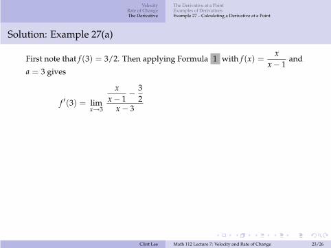
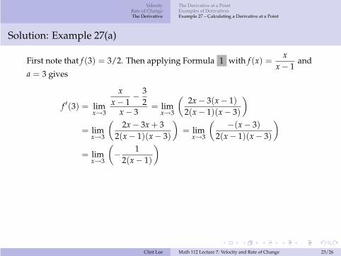
Solution: Example 27(a)
First note that f (3) = 3/2. Then applying Formula 1 with f (x) =x
x − 1and
a = 3 gives
f ′(3) =
Clint Lee Math 112 Lecture 7: Velocity and Rate of Change 23/26
VelocityRate of ChangeThe Derivative
The Derivative at a PointExamples of DerivativesExample 27 – Calculating a Derivative at a Point
Solution: Example 27(a)
First note that f (3) = 3/2. Then applying Formula 1 with f (x) =x
x − 1and
a = 3 gives
f ′(3) = limx→3
xx − 1
−32
x − 3
Clint Lee Math 112 Lecture 7: Velocity and Rate of Change 23/26
VelocityRate of ChangeThe Derivative
The Derivative at a PointExamples of DerivativesExample 27 – Calculating a Derivative at a Point
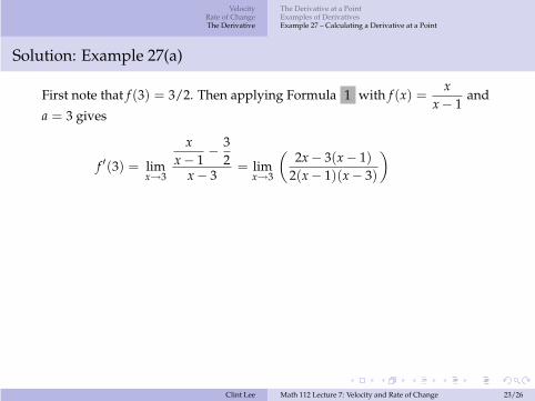
Solution: Example 27(a)
First note that f (3) = 3/2. Then applying Formula 1 with f (x) =x
x − 1and
a = 3 gives
f ′(3) = limx→3
xx − 1
−32
x − 3= lim
x→3
(
2x − 3(x − 1)
2(x − 1)(x − 3)
)
Clint Lee Math 112 Lecture 7: Velocity and Rate of Change 23/26
VelocityRate of ChangeThe Derivative
The Derivative at a PointExamples of DerivativesExample 27 – Calculating a Derivative at a Point
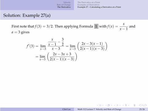
Solution: Example 27(a)
First note that f (3) = 3/2. Then applying Formula 1 with f (x) =x
x − 1and
a = 3 gives
f ′(3) = limx→3
xx − 1
−32
x − 3= lim
x→3
(
2x − 3(x − 1)
2(x − 1)(x − 3)
)
= limx→3
(
2x − 3x + 32(x − 1)(x − 3)
)
Clint Lee Math 112 Lecture 7: Velocity and Rate of Change 23/26
VelocityRate of ChangeThe Derivative
The Derivative at a PointExamples of DerivativesExample 27 – Calculating a Derivative at a Point
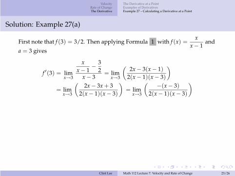
Solution: Example 27(a)
First note that f (3) = 3/2. Then applying Formula 1 with f (x) =x
x − 1and
a = 3 gives
f ′(3) = limx→3
xx − 1
−32
x − 3= lim
x→3
(
2x − 3(x − 1)
2(x − 1)(x − 3)
)
= limx→3
(
2x − 3x + 32(x − 1)(x − 3)
)
= limx→3
(
−(x − 3)
2(x − 1)(x − 3)
)
Clint Lee Math 112 Lecture 7: Velocity and Rate of Change 23/26
VelocityRate of ChangeThe Derivative
The Derivative at a PointExamples of DerivativesExample 27 – Calculating a Derivative at a Point
Solution: Example 27(a)
First note that f (3) = 3/2. Then applying Formula 1 with f (x) =x
x − 1and
a = 3 gives
f ′(3) = limx→3
xx − 1
−32
x − 3= lim
x→3
(
2x − 3(x − 1)
2(x − 1)(x − 3)
)
= limx→3
(
2x − 3x + 32(x − 1)(x − 3)
)
= limx→3
(
−(x − 3)
2(x − 1)(x − 3)
)
= limx→3
(
−1
2(x − 1)
)
Clint Lee Math 112 Lecture 7: Velocity and Rate of Change 23/26

VelocityRate of ChangeThe Derivative
The Derivative at a PointExamples of DerivativesExample 27 – Calculating a Derivative at a Point
Solution: Example 27(a)
First note that f (3) = 3/2. Then applying Formula 1 with f (x) =x
x − 1and
a = 3 gives
f ′(3) = limx→3
xx − 1
−32
x − 3= lim
x→3
(
2x − 3(x − 1)
2(x − 1)(x − 3)
)
= limx→3
(
2x − 3x + 32(x − 1)(x − 3)
)
= limx→3
(
−(x − 3)
2(x − 1)(x − 3)
)
= limx→3
(
−1
2(x − 1)
)
= −14
Clint Lee Math 112 Lecture 7: Velocity and Rate of Change 23/26
VelocityRate of ChangeThe Derivative
The Derivative at a PointExamples of DerivativesExample 27 – Calculating a Derivative at a Point
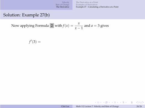
Solution: Example 27(b)
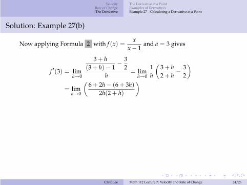
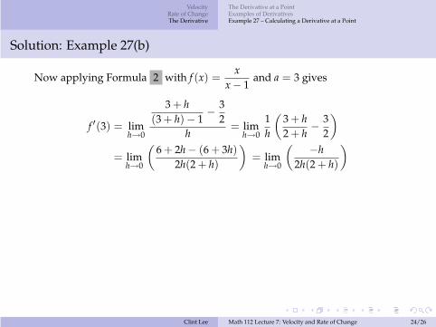
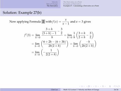
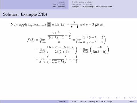
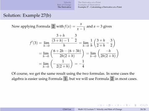
Now applying Formula 2 with f (x) =x
x − 1and a = 3 gives
f ′(3) =
Clint Lee Math 112 Lecture 7: Velocity and Rate of Change 24/26
VelocityRate of ChangeThe Derivative
The Derivative at a PointExamples of DerivativesExample 27 – Calculating a Derivative at a Point
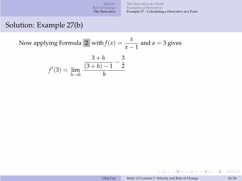
Solution: Example 27(b)
Now applying Formula 2 with f (x) =x
x − 1and a = 3 gives
f ′(3) = limh→0
3 + h(3 + h) − 1
−32
h
Clint Lee Math 112 Lecture 7: Velocity and Rate of Change 24/26
VelocityRate of ChangeThe Derivative
The Derivative at a PointExamples of DerivativesExample 27 – Calculating a Derivative at a Point
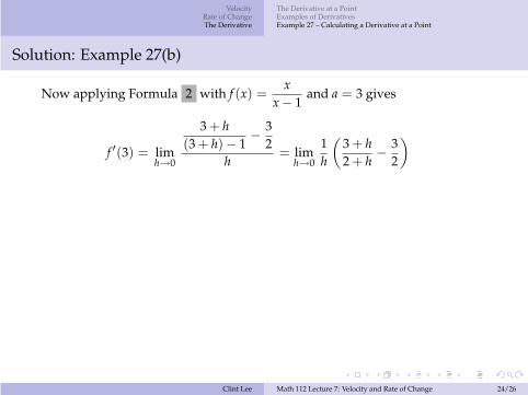
Solution: Example 27(b)
Now applying Formula 2 with f (x) =x
x − 1and a = 3 gives
f ′(3) = limh→0
3 + h(3 + h) − 1
−32
h= lim
h→0
1h
(
3 + h2 + h
−32
)
Clint Lee Math 112 Lecture 7: Velocity and Rate of Change 24/26
VelocityRate of ChangeThe Derivative
The Derivative at a PointExamples of DerivativesExample 27 – Calculating a Derivative at a Point
Solution: Example 27(b)
Now applying Formula 2 with f (x) =x
x − 1and a = 3 gives
f ′(3) = limh→0
3 + h(3 + h) − 1
−32
h= lim
h→0
1h
(
3 + h2 + h
−32
)
= limh→0
(
6 + 2h − (6 + 3h)
2h(2 + h)
)
= limh→0
(
−h2h(2 + h)
)
= limh→0
(
−1
2(2 + h)
)
= −14
Of course, we get the same result using the two formulas. In some cases thealgebra is easier using Formula 1 , but we will use Formula 2 in most cases.
Clint Lee Math 112 Lecture 7: Velocity and Rate of Change 24/26

VelocityRate of ChangeThe Derivative
The Derivative at a PointExamples of DerivativesExample 27 – Calculating a Derivative at a Point
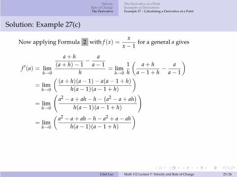
Solution: Example 27(c)
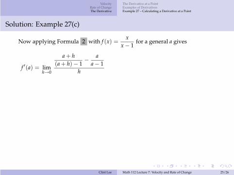
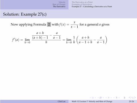
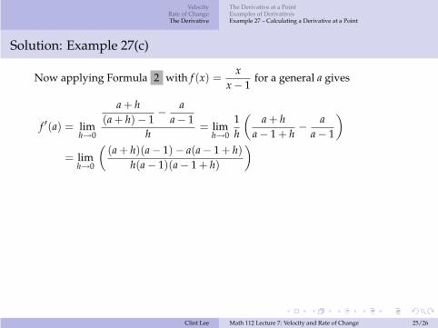
Now applying Formula 2 with f (x) =x
x − 1for a general a gives
f ′(a) =
Clint Lee Math 112 Lecture 7: Velocity and Rate of Change 25/26
VelocityRate of ChangeThe Derivative
The Derivative at a PointExamples of DerivativesExample 27 – Calculating a Derivative at a Point
Solution: Example 27(c)
Now applying Formula 2 with f (x) =x
x − 1for a general a gives
f ′(a) = limh→0
a + h(a + h) − 1
−a
a − 1h
= limh→0
1h
(
a + ha − 1 + h
−a
a − 1
)
= limh→0
(
(a + h)(a − 1) − a(a − 1 + h)
h(a − 1)(a − 1 + h)
)
Clint Lee Math 112 Lecture 7: Velocity and Rate of Change 25/26

VelocityRate of ChangeThe Derivative
The Derivative at a PointExamples of DerivativesExample 27 – Calculating a Derivative at a Point
Solution: Example 27(c)
Now applying Formula 2 with f (x) =x
x − 1for a general a gives
f ′(a) = limh→0
a + h(a + h) − 1
−a
a − 1h
= limh→0
1h
(
a + ha − 1 + h
−a
a − 1
)
= limh→0
(
(a + h)(a − 1) − a(a − 1 + h)
h(a − 1)(a − 1 + h)
)
= limh→0
(
a2− a + ah − h −
(
a2− a + ah
)
h(a − 1)(a − 1 + h)
)
Clint Lee Math 112 Lecture 7: Velocity and Rate of Change 25/26
VelocityRate of ChangeThe Derivative
The Derivative at a PointExamples of DerivativesExample 27 – Calculating a Derivative at a Point
Solution: Example 27(c)
Now applying Formula 2 with f (x) =x
x − 1for a general a gives
f ′(a) = limh→0
a + h(a + h) − 1
−a
a − 1h
= limh→0
1h
(
a + ha − 1 + h
−a
a − 1
)
= limh→0
(
(a + h)(a − 1) − a(a − 1 + h)
h(a − 1)(a − 1 + h)
)
= limh→0
(
a2− a + ah − h −
(
a2− a + ah
)
h(a − 1)(a − 1 + h)
)
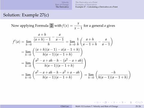
= limh→0
(
a2− a + ah − h − a2 + a − ah
h(a − 1)(a − 1 + h)
)
Clint Lee Math 112 Lecture 7: Velocity and Rate of Change 25/26
VelocityRate of ChangeThe Derivative
The Derivative at a PointExamples of DerivativesExample 27 – Calculating a Derivative at a Point
Solution: Example 27(c)
Now applying Formula 2 with f (x) =x
x − 1for a general a gives
f ′(a) = limh→0
a + h(a + h) − 1
−a
a − 1h
= limh→0
1h
(
a + ha − 1 + h
−a
a − 1
)
= limh→0
(
(a + h)(a − 1) − a(a − 1 + h)
h(a − 1)(a − 1 + h)
)
= limh→0
(
a2− a + ah − h −
(
a2− a + ah
)
h(a − 1)(a − 1 + h)
)
= limh→0
(
a2− a + ah − h − a2 + a − ah
h(a − 1)(a − 1 + h)
)
= limh→0
(
−hh(a − 1)(a − 1 + h)
)
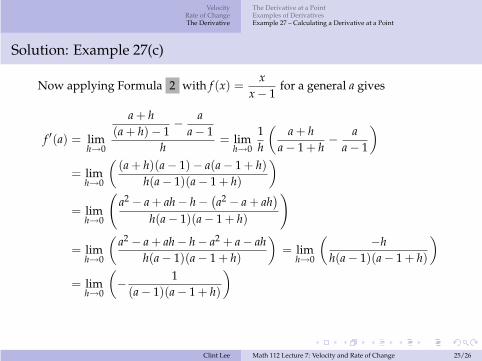
= limh→0
(
−1
(a − 1)(a − 1 + h)
)
Clint Lee Math 112 Lecture 7: Velocity and Rate of Change 25/26
VelocityRate of ChangeThe Derivative
The Derivative at a PointExamples of DerivativesExample 27 – Calculating a Derivative at a Point
Solution: Example 27(c)
Now applying Formula 2 with f (x) =x
x − 1for a general a gives
f ′(a) = limh→0
a + h(a + h) − 1
−a
a − 1h
= limh→0
1h
(
a + ha − 1 + h
−a
a − 1
)
= limh→0
(
(a + h)(a − 1) − a(a − 1 + h)
h(a − 1)(a − 1 + h)
)
= limh→0
(
a2− a + ah − h −
(
a2− a + ah
)
h(a − 1)(a − 1 + h)
)
= limh→0
(
a2− a + ah − h − a2 + a − ah
h(a − 1)(a − 1 + h)
)
= limh→0
(
−hh(a − 1)(a − 1 + h)
)
= limh→0
(
−1
(a − 1)(a − 1 + h)
)
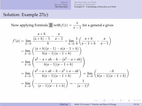
= −1
(a − 1)2
Clint Lee Math 112 Lecture 7: Velocity and Rate of Change 25/26
VelocityRate of ChangeThe Derivative
The Derivative at a PointExamples of DerivativesExample 27 – Calculating a Derivative at a Point
Solution: Example 27(c) – Continued
Substituting a = 3 into the formula for the derivative just derived gives
Clint Lee Math 112 Lecture 7: Velocity and Rate of Change 26/26
VelocityRate of ChangeThe Derivative
The Derivative at a PointExamples of DerivativesExample 27 – Calculating a Derivative at a Point
Solution: Example 27(c) – Continued
Substituting a = 3 into the formula for the derivative just derived gives
f ′(3) = −122 = −
14
which agrees with our calculations in parts (a) and (b).
Clint Lee Math 112 Lecture 7: Velocity and Rate of Change 26/26