Embed Size (px)
Citation preview
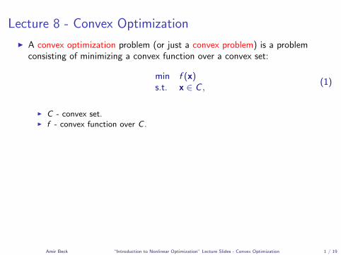
Lecture 8 - Convex Optimization
I A convex optimization problem (or just a convex problem) is a problemconsisting of minimizing a convex function over a convex set:
min f (x)s.t. x ∈ C ,
(1)
I C - convex set.I f - convex function over C .
I A functional form of a convex problem can written as
min f (x)s.t. gi (x) ≤ 0, i = 1, 2, . . . ,m
hj(x) = 0, j = 1, 2, . . . , p,
f , g1, . . . , gm : Rn → R are convex functions and h1, h2, . . . , hp : Rm → R areaffine functions.
I Note that the functional form does fit into the general formulation (1).
Amir Beck “Introduction to Nonlinear Optimization” Lecture Slides - Convex Optimization 1 / 19
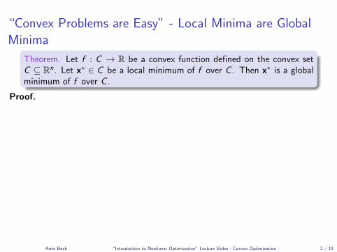
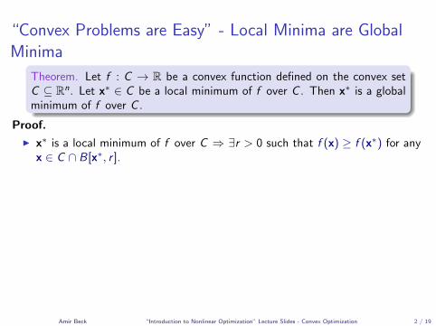
“Convex Problems are Easy” - Local Minima are GlobalMinima
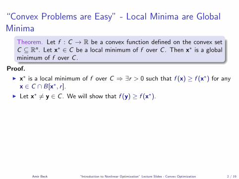
Theorem. Let f : C → R be a convex function defined on the convex setC ⊆ Rn. Let x∗ ∈ C be a local minimum of f over C . Then x∗ is a globalminimum of f over C .
Proof.
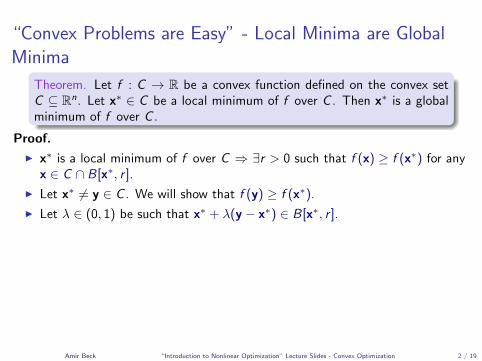
I x∗ is a local minimum of f over C ⇒ ∃r > 0 such that f (x) ≥ f (x∗) for anyx ∈ C ∩ B[x∗, r ].
I Let x∗ 6= y ∈ C . We will show that f (y) ≥ f (x∗).
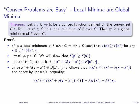
I Let λ ∈ (0, 1) be such that x∗ + λ(y − x∗) ∈ B[x∗, r ].
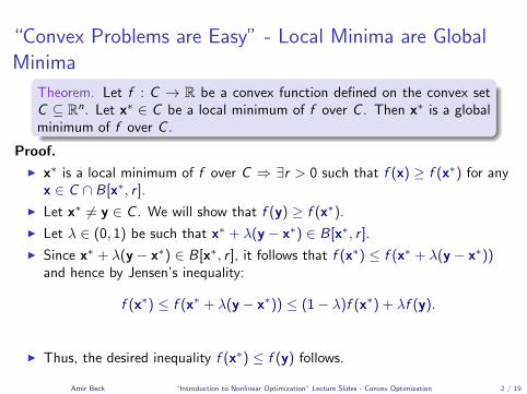
I Since x∗ + λ(y − x∗) ∈ B[x∗, r ], it follows that f (x∗) ≤ f (x∗ + λ(y − x∗))and hence by Jensen’s inequality:
f (x∗) ≤ f (x∗ + λ(y − x∗)) ≤ (1− λ)f (x∗) + λf (y).
I Thus, the desired inequality f (x∗) ≤ f (y) follows.
Amir Beck “Introduction to Nonlinear Optimization” Lecture Slides - Convex Optimization 2 / 19
“Convex Problems are Easy” - Local Minima are GlobalMinima
Theorem. Let f : C → R be a convex function defined on the convex setC ⊆ Rn. Let x∗ ∈ C be a local minimum of f over C . Then x∗ is a globalminimum of f over C .
Proof.
I x∗ is a local minimum of f over C ⇒ ∃r > 0 such that f (x) ≥ f (x∗) for anyx ∈ C ∩ B[x∗, r ].
I Let x∗ 6= y ∈ C . We will show that f (y) ≥ f (x∗).
I Let λ ∈ (0, 1) be such that x∗ + λ(y − x∗) ∈ B[x∗, r ].
I Since x∗ + λ(y − x∗) ∈ B[x∗, r ], it follows that f (x∗) ≤ f (x∗ + λ(y − x∗))and hence by Jensen’s inequality:
f (x∗) ≤ f (x∗ + λ(y − x∗)) ≤ (1− λ)f (x∗) + λf (y).
I Thus, the desired inequality f (x∗) ≤ f (y) follows.
Amir Beck “Introduction to Nonlinear Optimization” Lecture Slides - Convex Optimization 2 / 19
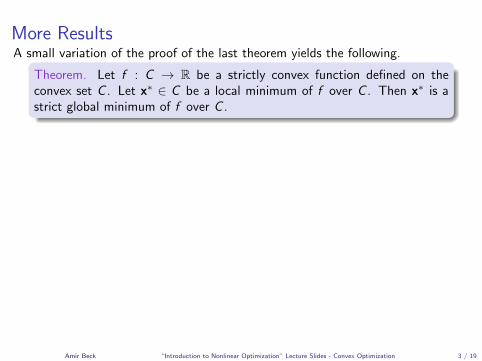
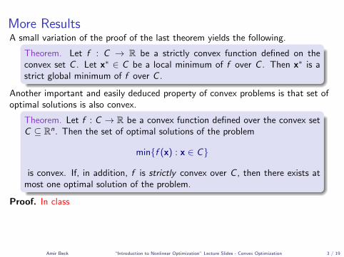
More ResultsA small variation of the proof of the last theorem yields the following.
Theorem. Let f : C → R be a strictly convex function defined on theconvex set C . Let x∗ ∈ C be a local minimum of f over C . Then x∗ is astrict global minimum of f over C .
Another important and easily deduced property of convex problems is that set ofoptimal solutions is also convex.
Theorem. Let f : C → R be a convex function defined over the convex setC ⊆ Rn. Then the set of optimal solutions of the problem
min{f (x) : x ∈ C}
is convex. If, in addition, f is strictly convex over C , then there exists atmost one optimal solution of the problem.
Proof. In class
Amir Beck “Introduction to Nonlinear Optimization” Lecture Slides - Convex Optimization 3 / 19
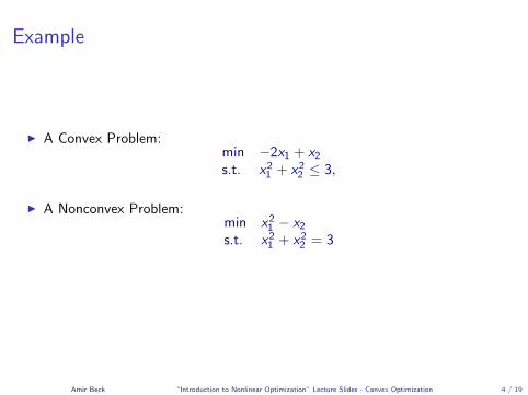
Example
I A Convex Problem:min −2x1 + x2s.t. x21 + x22 ≤ 3,
I A Nonconvex Problem:min x21 − x2s.t. x21 + x22 = 3
Amir Beck “Introduction to Nonlinear Optimization” Lecture Slides - Convex Optimization 4 / 19
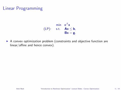
Linear Programming
(LP):min cTxs.t. Ax ≤ b,
Bx = g.
I A convex optimization problem (constraints and objective function arelinear/affine and hence convex).
I It is also equivalent to a problem of maximizing a convex (linear) functionsubject to a convex constraints set. Hence, if the feasible set is compact ansnonempty, then there exists at least one optimal solution which is an extremepoint=basic feasible solution.
I A more general result drops the compactness assumption and is often calledthe fundamental theorem of linear programming.
Amir Beck “Introduction to Nonlinear Optimization” Lecture Slides - Convex Optimization 5 / 19
Convex Quadratic Problems
I Convex quadratic problems are problems consisting of minimizing a convexquadratic function subject to affine constraints.
I The general form ismin xTQx + 2bTxs.t. Ax ≤ c,
Q ∈ Rn×n is positive semidefinite, b ∈ Rn,A ∈ Rm×n, c ∈ Rm.
Amir Beck “Introduction to Nonlinear Optimization” Lecture Slides - Convex Optimization 6 / 19
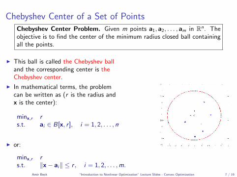
Chebyshev Center of a Set of PointsChebyshev Center Problem. Given m points a1, a2, . . . , am in Rn. Theobjective is to find the center of the minimum radius closed ball containingall the points.
I This ball is called the Chebyshev balland the corresponding center is theChebyshev center.
I In mathematical terms, the problemcan be written as (r is the radius andx is the center):
minx,r rs.t. ai ∈ B[x, r ], i = 1, 2, . . . ,m.
I or:
minx,r rs.t. ‖x− ai‖ ≤ r , i = 1, 2, . . . ,m.
Amir Beck “Introduction to Nonlinear Optimization” Lecture Slides - Convex Optimization 7 / 19
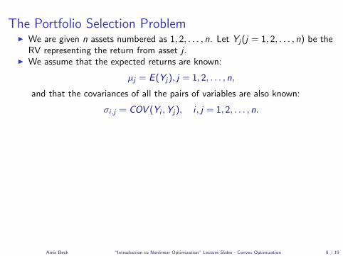
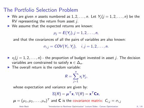
The Portfolio Selection ProblemI We are given n assets numbered as 1, 2, . . . , n. Let Yj(j = 1, 2, . . . , n) be the
RV representing the return from asset j .I We assume that the expected returns are known:
µj = E (Yj), j = 1, 2, . . . , n,
and that the covariances of all the pairs of variables are also known:
σi,j = COV (Yi ,Yj), i , j = 1, 2, . . . , n.
I xj(j = 1, 2, . . . , n) - the proportion of budget invested in asset j . The decisionvariables are constrained to satisfy x ∈ ∆n.
I The overall return is the random variable:
R =n∑
j=1
xjYj ,
whose expectation and variance are given by:
E(R) = µTx,V(R) = xTCx,
µ = (µ1, µ2, . . . , µn)T and C is the covariance matrix: Ci,j = σi,j
Amir Beck “Introduction to Nonlinear Optimization” Lecture Slides - Convex Optimization 8 / 19
The Portfolio Selection ProblemI We are given n assets numbered as 1, 2, . . . , n. Let Yj(j = 1, 2, . . . , n) be the
RV representing the return from asset j .I We assume that the expected returns are known:
µj = E (Yj), j = 1, 2, . . . , n,
and that the covariances of all the pairs of variables are also known:
σi,j = COV (Yi ,Yj), i , j = 1, 2, . . . , n.
I xj(j = 1, 2, . . . , n) - the proportion of budget invested in asset j . The decisionvariables are constrained to satisfy x ∈ ∆n.
I The overall return is the random variable:
R =n∑
j=1
xjYj ,
whose expectation and variance are given by:
E(R) = µTx,V(R) = xTCx,
µ = (µ1, µ2, . . . , µn)T and C is the covariance matrix: Ci,j = σi,jAmir Beck “Introduction to Nonlinear Optimization” Lecture Slides - Convex Optimization 8 / 19
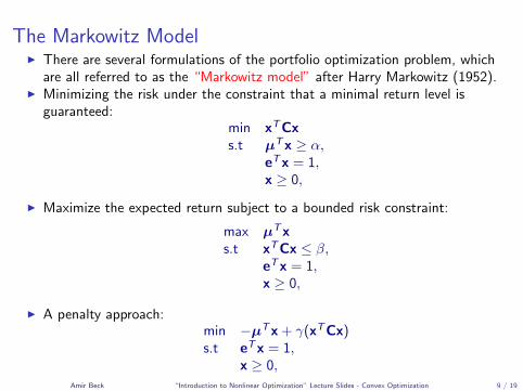
The Markowitz ModelI There are several formulations of the portfolio optimization problem, which
are all referred to as the “Markowitz model” after Harry Markowitz (1952).I Minimizing the risk under the constraint that a minimal return level is
guaranteed:min xTCxs.t µTx ≥ α,
eTx = 1,x ≥ 0,
I Maximize the expected return subject to a bounded risk constraint:
max µTxs.t xTCx ≤ β,
eTx = 1,x ≥ 0,
I A penalty approach:min −µTx + γ(xTCx)s.t eTx = 1,
x ≥ 0,
Amir Beck “Introduction to Nonlinear Optimization” Lecture Slides - Convex Optimization 9 / 19
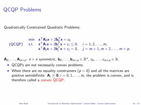
QCQP Problems
Quadratically Constrained Quadratic Problems:
(QCQP)min xTA0x + 2bT
0 x + c0s.t. xTAix + 2bT
i x + ci ≤ 0, i = 1, 2, . . . ,m,xTAjx + 2bT
j x + cj = 0, j = m + 1,m + 2, . . . ,m + p.
A0, . . . ,Am+p- n × n symmetric, b0, . . . ,bm+p ∈ Rn, c0, . . . , cm+p ∈ R.
I QCQPs are not necessarily convex problems.
I When there are no equality constrainers (p = 0) and all the matrices arepositive semidefinite: Ai � 0, i = 0, 1, . . . ,m, the problem is convex, and istherefore called a convex QCQP.
Amir Beck “Introduction to Nonlinear Optimization” Lecture Slides - Convex Optimization 10 / 19
The Orthogonal Projection OperatorI Definition. Given a nonempty closed convex set C , the orthogonal projection
operator PC : Rn → C is defined by
PC (x) = argmin{‖y − x‖2 : y ∈ C}.
The first important result is that the orthogonal projection exists and is unique.
The First Projection Theorem. Let C ⊆ Rn be a nonempty closed andconvex set. Then for any x ∈ Rn, the orthogonal projection PC (x) existsand is unique.
Proof. In class
Amir Beck “Introduction to Nonlinear Optimization” Lecture Slides - Convex Optimization 11 / 19

Examples
I C = Rn+.
PRn+
(x) = [x]+,
where [v]+ = (max{v1, 0}; max{v2, 0}; . . . ; max{vn, 0}).
I A box is a subset of Rn of the form
B = [`1, u1]× [`2, u2]× · · · × [`n, un] = {x ∈ Rn : `i ≤ xi ≤ ui},
where `i ≤ ui for all i = 1, 2, . . . , n.
[PB(x)]i =
ui xi ≥ uixi `i < xi < ui ,`i xi ≤ `i .
I C = B[0, r ].
PB[0,r ] =
{x ‖x‖ ≤ r ,r x‖x‖ ‖x‖ > r .
Amir Beck “Introduction to Nonlinear Optimization” Lecture Slides - Convex Optimization 12 / 19
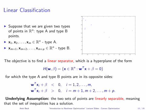
Linear Classification
I Suppose that we are given two typesof points in Rn: type A and type Bpoints.
I x1, x2, . . . , xm ∈ Rn - type A.
I xm+1, xm+2, . . . , xm+p ∈ Rn - type B.
0 0.5 1 1.5 2 2.5 3 3.5 4 4.5 50
0.5
1
1.5
2
2.5
3
3.5
4
4.5
The objective is to find a linear separator, which is a hyperplane of the form
H(w, β) = {x ∈ Rn : wTx + β = 0}
for which the type A and type B points are in its opposite sides:
wTxi + β < 0, i = 1, 2, . . . ,m,
wTxi + β > 0, i = m + 1,m + 2, . . . ,m + p.
Underlying Assumption: the two sets of points are linearly separable, meaningthat the set of inequalities has a solution.
Amir Beck “Introduction to Nonlinear Optimization” Lecture Slides - Convex Optimization 13 / 19
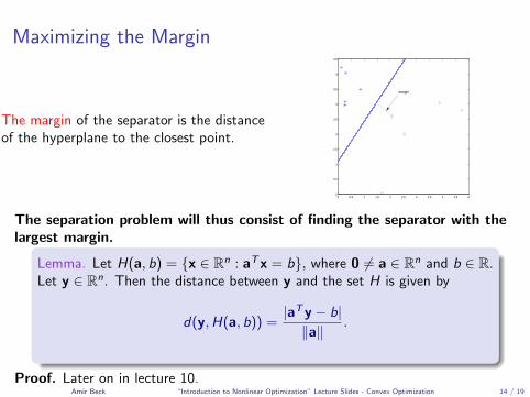
Maximizing the Margin
The margin of the separator is the distanceof the hyperplane to the closest point.
0 0.5 1 1.5 2 2.5 3 3.5 4 4.5 50
0.5
1
1.5
2
2.5
3
3.5
4
4.5
margin
The separation problem will thus consist of finding the separator with thelargest margin.
Lemma. Let H(a, b) = {x ∈ Rn : aTx = b}, where 0 6= a ∈ Rn and b ∈ R.Let y ∈ Rn. Then the distance between y and the set H is given by
d(y,H(a, b)) =|aTy − b|‖a‖
.
Proof. Later on in lecture 10.Amir Beck “Introduction to Nonlinear Optimization” Lecture Slides - Convex Optimization 14 / 19
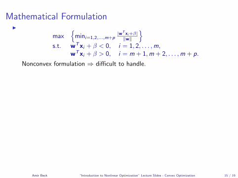
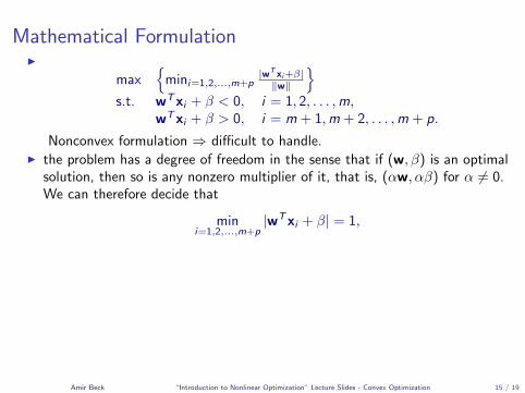
Mathematical FormulationI
max{
mini=1,2,...,m+p|wT xi+β|‖w‖
}s.t. wTxi + β < 0, i = 1, 2, . . . ,m,
wTxi + β > 0, i = m + 1,m + 2, . . . ,m + p.
Nonconvex formulation ⇒ difficult to handle.
I the problem has a degree of freedom in the sense that if (w, β) is an optimalsolution, then so is any nonzero multiplier of it, that is, (αw, αβ) for α 6= 0.We can therefore decide that
mini=1,2,...,m+p
|wTxi + β| = 1,
I Thus, the problem can be written as
max{
1‖w‖
}s.t. mini=1,2,...,m+p |wTxi + β| = 1,
wTxi + β < 0, i = 1, 2, . . . ,m,wTxi + β > 0, i = m + 1, 2, . . . ,m + p.
Amir Beck “Introduction to Nonlinear Optimization” Lecture Slides - Convex Optimization 15 / 19
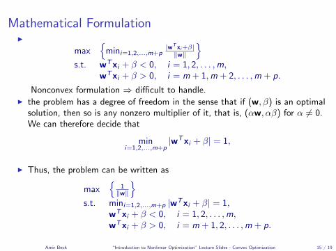
Mathematical FormulationI
max{
mini=1,2,...,m+p|wT xi+β|‖w‖
}s.t. wTxi + β < 0, i = 1, 2, . . . ,m,
wTxi + β > 0, i = m + 1,m + 2, . . . ,m + p.
Nonconvex formulation ⇒ difficult to handle.I the problem has a degree of freedom in the sense that if (w, β) is an optimal
solution, then so is any nonzero multiplier of it, that is, (αw, αβ) for α 6= 0.We can therefore decide that
mini=1,2,...,m+p
|wTxi + β| = 1,
I Thus, the problem can be written as
max{
1‖w‖
}s.t. mini=1,2,...,m+p |wTxi + β| = 1,
wTxi + β < 0, i = 1, 2, . . . ,m,wTxi + β > 0, i = m + 1, 2, . . . ,m + p.
Amir Beck “Introduction to Nonlinear Optimization” Lecture Slides - Convex Optimization 15 / 19

Mathematical Formulation Contd.
I
min 12‖w‖
2
s.t. mini=1,2,...,m+p |wTxi + β| = 1,wTxi + β ≤ −1, i = 1, 2, . . . ,m,wTxi + β ≥ 1, i = m + 1, 2, . . . ,m + p,
I The first constraint can be dropped (why?)
min 12‖w‖
2
s.t. wTxi + β ≤ −1, i = 1, 2, . . . ,m,wTxi + β ≥ 1, i = m + 1,m + 2, . . . ,m + p.
Convex Formulation.
Amir Beck “Introduction to Nonlinear Optimization” Lecture Slides - Convex Optimization 16 / 19
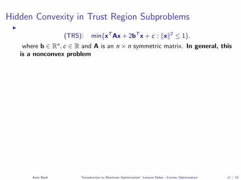
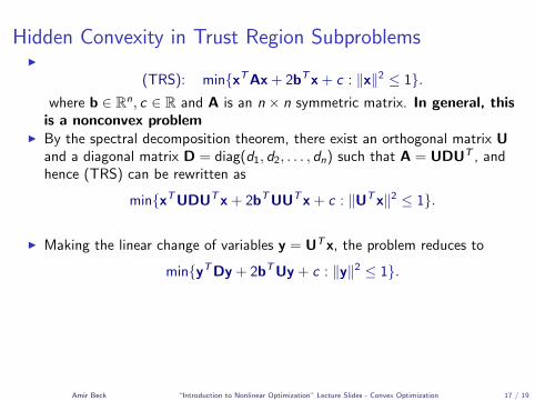
Hidden Convexity in Trust Region SubproblemsI
(TRS): min{xTAx + 2bTx + c : ‖x‖2 ≤ 1}.where b ∈ Rn, c ∈ R and A is an n × n symmetric matrix. In general, this
is a nonconvex problem
I By the spectral decomposition theorem, there exist an orthogonal matrix Uand a diagonal matrix D = diag(d1, d2, . . . , dn) such that A = UDUT , andhence (TRS) can be rewritten as
min{xTUDUTx + 2bTUUTx + c : ‖UTx‖2 ≤ 1}.
I Making the linear change of variables y = UTx, the problem reduces to
min{yTDy + 2bTUy + c : ‖y‖2 ≤ 1}.
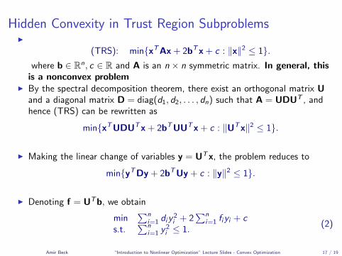
I Denoting f = UTb, we obtain
min∑n
i=1 diy2i + 2
∑ni=1 fiyi + c
s.t.∑n
i=1 y2i ≤ 1.
(2)
Amir Beck “Introduction to Nonlinear Optimization” Lecture Slides - Convex Optimization 17 / 19
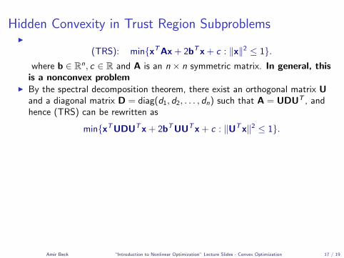
Hidden Convexity in Trust Region SubproblemsI
(TRS): min{xTAx + 2bTx + c : ‖x‖2 ≤ 1}.where b ∈ Rn, c ∈ R and A is an n × n symmetric matrix. In general, this
is a nonconvex problemI By the spectral decomposition theorem, there exist an orthogonal matrix U
and a diagonal matrix D = diag(d1, d2, . . . , dn) such that A = UDUT , andhence (TRS) can be rewritten as
min{xTUDUTx + 2bTUUTx + c : ‖UTx‖2 ≤ 1}.
I Making the linear change of variables y = UTx, the problem reduces to
min{yTDy + 2bTUy + c : ‖y‖2 ≤ 1}.
I Denoting f = UTb, we obtain
min∑n
i=1 diy2i + 2
∑ni=1 fiyi + c
s.t.∑n
i=1 y2i ≤ 1.
(2)
Amir Beck “Introduction to Nonlinear Optimization” Lecture Slides - Convex Optimization 17 / 19
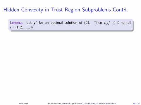
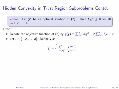
Hidden Convexity in Trust Region Subproblems Contd.
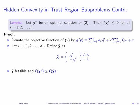
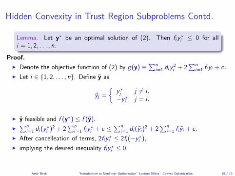
Lemma. Let y∗ be an optimal solution of (2). Then fiy∗i ≤ 0 for all
i = 1, 2, . . . , n.
Proof.
I Denote the objective function of (2) by g(y) ≡∑n
i=1 diy2i + 2
∑ni=1 fiyi + c .
I Let i ∈ {1, 2, . . . , n}. Define y as
yj =
{y∗j j 6= i ,−y∗i j = i .
I y feasible and f (y∗) ≤ f (y).
I∑n
i=1 di (y∗i )2 + 2
∑ni=1 fiy
∗i + c ≤
∑ni=1 di (yi )
2 + 2∑n
i=1 fi yi + c .
I After cancelleation of terms, 2fiy∗i ≤ 2fi (−y∗i ),
I implying the desired inequality fiy∗i ≤ 0.
Amir Beck “Introduction to Nonlinear Optimization” Lecture Slides - Convex Optimization 18 / 19

Hidden Convexity in Trust Region Subproblems Contd.
Lemma. Let y∗ be an optimal solution of (2). Then fiy∗i ≤ 0 for all
i = 1, 2, . . . , n.
Proof.
I Denote the objective function of (2) by g(y) ≡∑n
i=1 diy2i + 2
∑ni=1 fiyi + c .
I Let i ∈ {1, 2, . . . , n}. Define y as
yj =
{y∗j j 6= i ,−y∗i j = i .
I y feasible and f (y∗) ≤ f (y).
I∑n
i=1 di (y∗i )2 + 2
∑ni=1 fiy
∗i + c ≤
∑ni=1 di (yi )
2 + 2∑n
i=1 fi yi + c .
I After cancelleation of terms, 2fiy∗i ≤ 2fi (−y∗i ),
I implying the desired inequality fiy∗i ≤ 0.
Amir Beck “Introduction to Nonlinear Optimization” Lecture Slides - Convex Optimization 18 / 19
Hidden Convexity in Trust Region Subproblems Contd.
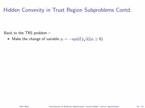
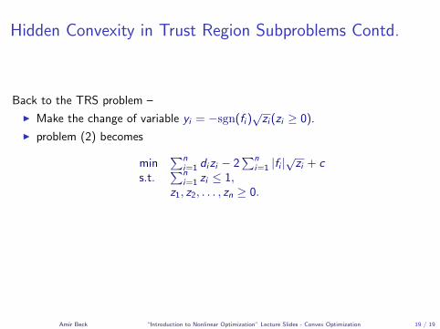
Back to the TRS problem –
I Make the change of variable yi = −sgn(fi )√zi (zi ≥ 0).
I problem (2) becomes
min∑n
i=1 dizi − 2∑n
i=1 |fi |√zi + c
s.t.∑n
i=1 zi ≤ 1,z1, z2, . . . , zn ≥ 0.
I convex optimization problem.
Amir Beck “Introduction to Nonlinear Optimization” Lecture Slides - Convex Optimization 19 / 19
Hidden Convexity in Trust Region Subproblems Contd.
Back to the TRS problem –
I Make the change of variable yi = −sgn(fi )√zi (zi ≥ 0).
I problem (2) becomes
min∑n
i=1 dizi − 2∑n
i=1 |fi |√zi + c
s.t.∑n
i=1 zi ≤ 1,z1, z2, . . . , zn ≥ 0.
I convex optimization problem.
Amir Beck “Introduction to Nonlinear Optimization” Lecture Slides - Convex Optimization 19 / 19