Embed Size (px)
Citation preview

Preprint typeset in JHEP style - HYPER VERSION
Lecture 8: Lie Algebras from Lie Groups
Gregory W. Moore
Abstract: Not updated since November 2009. March 27, 2018

Contents-TOC-
1. Introduction 2
2. Geometrical approach to the Lie algebra associated to a Lie group 2
2.1 Lie’s approach 2
2.2 Left-invariant vector fields and the Lie algebra 4
2.2.1 Review of some definitions from differential geometry 4
2.2.2 The geometrical definition of a Lie algebra 5
3. The exponential map 8
4. Baker-Campbell-Hausdorff formula 11
4.1 Statement and derivation 11
4.2 Two Important Special Cases 17
4.2.1 The Heisenberg algebra 17
4.2.2 All orders in B, first order in A 18
4.3 Region of convergence 19
5. Abstract Lie Algebras 19
5.1 Basic Definitions 19
5.2 Examples: Lie algebras of dimensions 1, 2, 3 23
5.3 Structure constants 25
5.4 Representations of Lie algebras and Ado’s Theorem 26
6. Lie’s theorem 28
7. Lie Algebras for the Classical Groups 34
7.1 A useful identity 35
7.2 GL(n, k) and SL(n, k) 35
7.3 O(n, k) 38
7.4 More general orthogonal groups 38
7.4.1 Lie algebra of SO∗(2n) 39
7.5 U(n) 39
7.5.1 U(p, q) 42
7.5.2 Lie algebra of SU∗(2n) 42
7.6 Sp(2n) 42
8. Central extensions of Lie algebras and Lie algebra cohomology 46
8.1 Example: The Heisenberg Lie algebra and the Lie group associated to a
symplectic vector space 47
8.2 Lie algebra cohomology 48
– 1 –

9. Left-invariant differential forms 50
10. The Maurer-Cartan equation 51
11. Examples 53
11.1 SU(2) 53
11.1.1 The Heisenberg group 55
12. Metrics on Lie groups 56
12.1 Simple Lie groups and the index of a representation 58
12.2 Metrics on abelian groups 60
12.3 Geodesics 60
12.4 Compact and noncompact real forms: The signature of the CK metric 60
12.5 Example: SL(2, R) 61
13. Some Remarks on Infinite Dimensional Lie Algebras 62
13.1 Generalities 62
13.2 Groups of operators on Hilbert space 62
13.3 Gauge Groups 62
13.3.1 Loop algebras 62
13.4 Diffeomorphism Groups 63
13.4.1 Gravity in 1+1 dimensions 64
13.4.2 The exponential map for Diff(S1) 66
1. Introduction
Quite generally, when one is confronted with a nonlinear object or phenomenon it is often
useful to reduce the problem to a linear problem, at the cost of restricting the domain of
applicability.
Lie groups are not linear – they are curved manifolds. If one chooses coordinates then
the group multiplication law is, in general, given by a complicated power series in the
coordinates.
Nevertheless, Lie’s theorem reduces many questions about Lie groups to questions
about Lie algebras. Questions about curved manifolds turn out to be equivalent to questions
about linear algebra. This is a profound simplification, and it leads to a very rich theory.
2. Geometrical approach to the Lie algebra associated to a Lie group
2.1 Lie’s approach
A good way to approach the subject is the way Sophus Lie did himself. A Lie group is a
group with continuous (or smooth) parameters. We convert the associativity of the group
law into a differential equation, and study the integrability of that differential equation.
– 2 –

Suppose x1, . . . , xn are coordinates in a neighborhood U of 1G, where n = dimG. We
take x = 0 to correspond to 1G. Thus, we have a smooth parametrization of group elements
g(x). The product of two group elements near the identity will be another group element
near the identity. Thus, there is a neighborhood U ′ ⊂ U so that if g(x), g(y) ∈ U ′ then we
can write the group law as:
g(x)g(y) = g(φ(x, y)) (2.1) eq:grplaw
for some smooth functions φi(x, y), i = 1, . . . n.
The group laws can be expressed in terms of φ:
1. Associativity:
φ(x, φ(y, z)) = φ(φ(x, y), z) (2.2) eq:associa
2. Identity: φ(0, x) = φ(x, 0) = x
3. Inverse: φ(x, x0) = φ(x0, x) = 0 is solvable for a unique x in terms of x0.
Now, let us differentiate the associativity condition (2.2) with respect to the zk:
∂φi(x, φ(y, z))
∂φj(y, z)
∂φj(y, z)
∂zk=∂φi
∂zk(φ(x, y), z) (2.3) eq:slieone
where repeated indices are summed.
Now define an n× n matrix function of one variable:
uik(x) :=∂φi(x, y)
∂yk
∣∣∣∣y=0
(2.4) eq:defnsu
Then, setting z = 0 in (2.3) gives
∂φi(x, y)
∂yjujk(y) = uik(φ(x, y)) (2.5) eq:lieseq
Note that (2.5) is equivalent to the equality of first order differential operators:
ujk(y)∂
∂yj= uik(φ(x, y))
∂
∂φi(2.6) eq:livfone
Here we are holding x fixed and viewing yi → φi(x, y) as a nonlinear change of coor-
dinates. Nevertheless the equation is true for any x and hence we can write (2.6) as
ujk(y)∂
∂yj= uik(φ)
∂
∂φi(2.7) eq:livfonep
Now, (2.7) is a remarkable equation because the LHS depends only on y and the RHS
depends only on φ. We will apply this observation in one moment.
A second observation is that if we denote
Ik(y) := ujk(y)∂
∂yj(2.8) eq:invtvf
then we can compute
– 3 –

[Ik(y), Im(y)] =(ujk∂ju
lm − ujm∂jul k
) ∂∂yl
=(ujk∂ju
lm − ujm∂jul k
)(utr,−1) p
l Ip(y)
:= fpkm(y)Ip(y)
(2.9) eq:commis
Now, by (2.7) Ik(y) = Ik(φ) so it follows that fpmk(y) = fpmk(φ), and since φ = φ(x, y)
with arbitrary x, it follows that fpmk(y) is constant ! Let us consider the finite-dimensional
vector space spanned by the first order differential operators) Ik(y) in (2.8). That is,
we consider the linear combinations of the Ik(y) with constant (real) coefficients. Note
that this vector space is closed under commutator. We denote this vector space L(G) or
sometimes g. Note that
dimG = dimL(G) (2.10)
On the LHS we have the dimension of a manifold, and on the RHS the dimension of a
vector space. Moreover, it follows from general properties of differential operators that if
X1, X2, X3 are any three vector fields in L(G) then
[[X1, X2], X3] + [[X3, X1], X2] + [[X2, X3], X1] = 0 (2.11) eq:jacobi
This crucial identity is known as the Jacobi identity.
These are the crucial properties which are abstracted into the general definition:
Definition : An abstract Lie algebra g over a field k is a vector space over k together
with a product (v1, v2)→ [v1, v2] ∈ g, such that for all v1, v2, v3,∈ g α, β ∈ k.
1.) [v1, v2] = −[v2, v1]
2.) [αv1 + βv2, v3] = α[v1, v3] + β[v2, v3]
3.) [[v1, v2], v3] + [[v3, v1], v2] + [[v2, v3], v1] = 0.
2.2 Left-invariant vector fields and the Lie algebra
We will now rephrase Lie’s argument in the language of modern differential geometry.
2.2.1 Review of some definitions from differential geometry
Tangent vectors are directional derivatives along paths. If we imagine M ⊂ RN then we
literally take a tangent plane. In general if p ∈ M let C1(p) be the functions defined in
some neighborhood of p ∈M , which are differentiable at p. A directional derivative along
a curve γ(t) such that γ(0) = p is a linear functional on this space defined by
γ(f) :=d
dt|t=0f(γ(t)) (2.12)
Then the space of tangent vectors at p, TpM , is the linear span of these linear functionals
C1(p)→ R. A vector field is a continuous system of tangent vectors.
– 4 –

Now suppose that φ : M1 → M2 is a map between manifolds. Let us study how
geometric objects behave with respect to such maps.
First of all, functions are contravariant. That is we define the pullback on functions
φ∗ : Fun(M2)→ Fun(M1) (2.13)
by φ∗(f) = f φ. Here Fun(M) is the space of all (say, continuous) functions from M to
(say) the real numbers.
By contrast, vectorfields push forward :
φ∗ : TpM1 → Tφ(p)M2 (2.14)
the definition is that φ∗(γ) is the directional derivative along the curve φ(γ(t)).
Two facts we will need below are:
• The commutator of two first-order differential operators is a first order differential
operator. This defines the commutator of two vector fields:
[ξ1, ξ2] (2.15)
Thus, V ect(M) is a Lie algebra, for any manifold M . It is infinite-dimensional. It is not
difficult to show that
φ∗[ξ1, ξ2] = [φ∗(ξ1), φ∗(ξ2)] (2.16)
•Vector fields act on functions to produce new functions. From the above definitions it
follows that:
φ∗(V )(f) = V (φ∗(f)) (2.17)
Exercise
In general, functions do not push forward. They only pull back. However, if φ is an
invertible map between manifolds show that it makes sense to define φ∗(f) = f φ−1. This
is used when pushing forward the product of a function and a vector field, fV in the next
section.
2.2.2 The geometrical definition of a Lie algebra
Definition. A left translation, or right translation by an element g ∈ G is the diffeomor-
phism:
Lg : G→ G h 7→ g · hRg : G→ G h 7→ h · g−1
(2.18) eq:leftrighttrns
– 5 –

Exercise
Show that Lg, Rg define injections of groups G → Diff(G).
Now we introduce the important idea of left and right invariance: A left-invariant
function satisfies:
L∗g(f) = f (2.19) eq:lftinvfun
for all g ∈ G. Of course, this just means that f is constant, because if we evaluate
(2.19) at g = 1 then
L∗g(f)|h=1 = f |h=1 ⇒ f(g · 1) = f(1) (2.20) eq:lftinvfunp
However, the notion of left- or right- invariant tensors still leaves room for very inter-
esting examples.
Definition. A vector field ξ ∈ V ect(G) is left (or right) invariant if
(Lg0)∗(ξg) = ξg0·g
(Rg0)∗(ξg) = ξgg−10
(2.21) eq:livr
is satisfied for all g, g0 ∈ G, respectively.
The picture is: For a general vector field ξg is the directional derivative at g to some
curve γg(t) going through g, while ξg0g is the directional derivative of some -a priori unre-
lated - curve γg0g(t) going through g0g. Then the condition of left-invariance:
(Lg)∗(ξg) = ξg0g (2.22)
means γg0g(t) has the same directional derivative at t = 0 as the curve g0 · γg(t).We now recognize our first order operators Ik(y) defined in (2.8) as vector fields on the
group G. The equation (2.7) is the statement that these are left-invariant vector fields.
Now, let us return to the general situation. Note that if ξ1, ξ2 are two LIVF’s then
(Lg)∗[ξ1, ξ2] = [(Lg)∗(ξ1), (Lg)∗(ξ2)] = [ξ1, ξ2] (2.23)
This leads to the
Geometric definition of the Lie algebra: We define the Lie algebra L(G) of a Lie
group G to be the Lie algebra of left invariant vector fields on G.
Examples
• G = U(1). The general vector field on U(1) is
ξ = f(θ)d
dθ(2.24)
– 6 –

Left invariant (and right-invariant) vector fields satisfy f(θ + θ0) = f(θ) for all θ0. That
is, f(θ) must be constant.
• G = GL(n, k), k = R,C. We can choose as global coordinates on the manifold
the matrix elements gij of g ∈ G. Introduce an n × n matrix of vector fields ∂∂g whose
components are: ( ∂∂g
)ij
:=∂
∂gij(2.25)
( ∂∂gij
)g0 is the directional derivative along the curve g0 + teij where eij is a matrix unit.
Note that if g0 is invertible then this curve is indeed in GL(n, k) for sufficiently small |t|.One computes
(Lg0)∗(∂
∂g) = gtr0 ·
∂
∂g(2.26)
where matrix multiplication on the RHS is understood. To do this, let fkl(g) = gkl be the
function which picks out a matrix element. Then
(Lg0)∗(∂
∂gij)(fkl) =
∂
∂gijfkl Lg0 =
∂
∂gij
∑s
(g0)ksfsl = (g0)kiδj,l (2.27)
Therefore,
(Lg0)∗(∂
∂gij|g) =
∑k
(g0)ki∂
∂gkj|g0g (2.28)
Therefore
ξij := (gtr∂
∂g)ij =
∑k
gki( ∂∂g
)kj
(2.29)
is a matrix of left-invariant vector fields on GL(n). Proof:
(Lg0)∗(gtr ∂
∂g) = (g−1
0 g)trgtr0 ·∂
∂g
= gtr · ∂∂g
(2.30)
The n2 vector fields ξij are linearly independent (simply consider their values at g0 = 1)
and form a basis for all LIVF’s on GL(n), by an argument given below. Finally, note that
by direct computation we find
[ξij , ξkl] = δjkξil − δliξkj (2.31) eq:glsc
and the structure constants are indeed constant.
Returning to the general case, let us now suppose ξ is a LIVF. Then ξg = (Lg)∗(ξ1),
so a LIVF is completely determined by its value at g = 1, and hence we can identify L(G)
with the tangent space at g = 1: L(G) ∼= T1(G), at least, as a vector space. Conversely,
given a tangent vector X ∈ T1(G). Then to X ∈ T1(G) we can associate a curve γX(t)
through g = 1 whose tangent vector at g = 1 is X. (As we will see below for a matrix group
we can take γX(t) to be the curve exp[tX] where we literally exponentiate the matrix. ) If
– 7 –

G is a Lie group, then the right action of G on itself defines a global system of left-invariant
vector fields on G as follows: If X ∈ T1(G) is the directional derivative along a curve γX(t)
passing through g = 1 then then the curves γX,g(t) := gγX(t) through g have directional
derivatives defining a vector field ξ(X) ∈ TgG. This vector field is left-invariant, and in
this way we define the map from T1G to the left-invariant vector fields on G.
The left-invariant vector fields ξ(X) are called the fundamental vector fields on G.
Every LIVF of G is of the form ξ(X) for some unique X (indeed X = ξ1) so we can define
[X,Y ] ∈ T1G by
[ξ(X), ξ(Y )] = ξ([X,Y ]) (2.32) eq:LieTone
This defines T1G as a Lie algebra, and then ξ defines a homomorphism of Lie algebras
T1(G)→ V ect(G).
To get a better feel for these vector fields consider again the example of G = GL(n,F).
The Lie algebra is g = Matn(F). Let eij be the matrix unit with a 1 in the ith row and jth
column, and zero in all other matrix elements. Then one easily computes the vector field
by considering the curve gexp[teij ]:
ξ(eij) =n∑k=1
gki∂
∂gkj(2.33) eq:vertcli
where we are regarding the matrix elements gij as coordinates on the group. Thus the
fundamental vector fields on G are just the vector fields ξij we examined above.
Then, combining (2.31) and (2.32) we have
ξ([eij , ei′j′ ]
)= [ξ(eij), ξ(ei′j′)] = δji′ξ(eij′)− δij′ξ(ei′j) (2.34)
and we conclude that [eij , ei′j′ ] coincides with matrix commutator, as it should.
If G ⊂ GL(n,F) is a subgroup of a matrix group then the matrix elements gij are not
all independent, so some vectors ∂∂gkj
will be expressed in terms of others. Put differently,
a path such at 1 + teij will not be a path within the matrix subgroup in general. These
linear dependences are most easily computed using the dual cotangent space T ∗1G and the
Maurer-Cartan form, as discussed below.
Exercise
Write out the right-invariant vector fields on GL(n,F).
3. The exponential map
We have discussed in chapter 2 how to exponentiate matrices. We would now like to
generalize this notion to define a map
exp : L(G)→ G (3.1)
– 8 –

Since not all Lie groups are matrix groups it will be a little more abstract.
Consider a homomorphism f : R→ GL(n,R). Such a map must satisfy
d
dtf(t) = lim
h→0h−1[f(t+ h)− f(t)]
= limh→0
h−1[f(h)− 1]f(t)
= Af(t)
(3.2)
so f(t) is the unique solution to this differential equation with f(0) = 1. We write
f(t) = etA (3.3)
Recall that for A ∈Mn(k) k = R or C, we defined
expA :=∑j≥0
Aj
j!∈Mn(k) (3.4)
defines the exponential of a matrix. In general any function defined by a power series can
be evaluated for matrix arguments, as above.
In a sufficiently small neighborhood U of 0 the map exp : Mn(R) → GL(n,R) is
invertible with
logg = −∞∑k=1
(1− g)k/k (3.5)
as its unique inverse.
As we have said, not all Lie groups are matrix groups. So we define exp more generally
(and more intrinisically) as follows:
Theorem: If G is a Lie group there is a 1-1 correspondence between the tangent space
T1G and group homomorphisms f : R→ G (aka “1-parameter subgroups”).
Proof : A homomorphism clearly determines a tangent vector X ∈ T1G. Conversely,
given a tangent vector X ∈ T1G we consider the left-invariant vector field ξ(X). We study
the tangent curves to ξ(X): these are curves γX(t) such that
γX(t) = ξ(X)|γX(t). (3.6) eq:tangentcurve
We would like to show that the tangent curve through g = 1 defines a group homo-
morphism of R into G.
We can take the tangent curve to satisfy γX(0) = 1G. Equation (3.6) is just an
ODE. By the theory of ODE’s we know that we can find γX(t) on a sufficiently small
neighborhood t ∈ (−ε, ε). Now consider a t0 in this interval. Similarly, we can study this
differential equation near γX(t0). Now γX(t+ t0) and γX(t0)γX(t) are both solutions, since
ξ(X) is left-invariant. By the uniqueness of solutions to ODE’s
γX(t+ t0) = γX(t0)γX(t) (3.7)
– 9 –

for t, t0, t+ t0 in the interval, so γX(t) is a local homomorphism. To extend the definition
of γX(t) to large values of t we take
γX(t) := (γX(t/n))n (3.8) eq:largetee
for sufficiently large n. (Exercise: Show that it doesn’t matter what n you pick.) ♠Evaluation of γX(t) at t = 1 defines the map
exp : T1G→ G (3.9)
whose derivative at 1G is the identity. In this way we define exp, even if G is not a matrix
group.
Remarks:
• exp : R→ U(1) given by x→ e2πix shows that exp is in general not 1-1.
•A Lie group can be given the structure of a Riemannian manifold in a canonical
way. The geodesics through 1G are precisely the 1-parameter subgroups. For a compact
Lie group, we get a complete Riemannian manifold, and a general theorem of differential
geometry shows that any two points on a complete Riemannian manifold can be joined by
a geodesic. Therefore, for a compact Lie group, exp is onto.
• For a noncompact Lie group exp need not be onto. We will give counterexamples
when we survey the Lie algebras of matrix groups below.
• As we will see, finite dimensional Lie algebras can be exponentiated to form Lie
groups. However, there exist examples of Lie algebras which cannot be “exponentiated”
to form Lie groups.
Exercise
Show that the choice of n does not matter in (3.8).
Exercise Exponentials and inverses
a.) Show that for the abstract exp map we have:
eAe−A = 1 (3.10)
for any A ∈ g.
b.) Define Ad(G) on g ..... *** NEED SOME DETAILS *** Show that
exp[BAB−1] = Bexp(A)B−1 (3.11)
– 10 –

4. Baker-Campbell-Hausdorff formulasec:sBCH
The exponential map is neither one-one nor onto in general. However, for a finite dimen-
sional Lie group, in a sufficiently small neighborhood of the identity 1G ∈ U2 ⊂ G and
0 ∈ U1 ⊂ T1G, exp : U1 → U2 is 1-1 and onto.
It is therefore natural to ask what the full group law looks like in terms of the linear
space g := T1G. Thus we would like to express
C(A,B) = logeAeB (4.1)
in terms of A,B.
If we imagine A,B are sufficiently small (we will say they are “order one”) then we
can expand in Taylor series
C(A,B) = A+B +1
2b(A,B) + · · · (4.2)
where b(A,B) ∈ g are the terms of order 2 and · · · are the terms of order ≥ 3. The factor
of 12 is for later convenience. 1
Since C(A, 0) = A and C(0, B) = B, b(A,B) has no terms of order A2 or B2 and hence
is a bilinear map:
b : g× g→ g (4.3)
Moreover, since exp(−A) = (exp(A))−1 we have C(−B,−A) = −C(A,B) and therefore
b(A,B) = −b(B,A), that is, b is skew-symmetric. Thus, working infinitesimally, we derive
the Lie product on T1G.
Now, the amazing thing about Lie groups is that
the entire Taylor series C(A,B) can be expressed solely in terms of b.
The formula that does this is known as the BCH formula, and we will now derive it
for the case of matrix groups in the next section.
4.1 Statement and derivation
The BCH formula allows us to understand the Lie group operation in terms of the matrices
in the exponential. It also provides a convenient way to understand the relationship between
Lie groups and Lie algebras. 2
The problem we want to solve in this section is:
Let A,B be n× n matrices. Find a matrix C such that eC = eAeB where C is expressed as a (possibly infinite) series in A,B.
1To be more precise, we can introduce parameters t1, t2 which are real and small and consider the
multiplication of exp[t1A]exp[t2B]. The “degree” is the total degree of t1 and t2 in the Taylor expansion.2The proof in this section follows Miller, Symmetry Groups and their applications.
– 11 –

The series we will obtain is convergent for “small” matrices. We can make this precise
by, for example defining ‖ A ‖= max|aij | and demanding that ‖ A ‖, ‖ B ‖ be sufficiently
small. We comment on the radius of convergence below.
Lemma 1: Let A be a constant matrix in t. Then
d
dtetA = AetA = etAA (4.4)
Proof: Series expansion. ♠To state the next lemma we introduce some notation:
Definition 4.1: For A ∈ Mn(k) we denote by Ad(A) the linear transformation Mn(k)→Mn(k) defined by
Ad(A) : B 7→ [A,B] (4.5)
We also denote:
(Ad(A))mB =
m times︷ ︸︸ ︷[A, [A, · · · [A,B] · · · ] (4.6)
where there are m commutators on the RHS.
Lemma 2:
eABe−A = eAdA(B) = Σ(AdA)j
j!B
= B + [A,B] +1
2[A, [A,B]] + · · ·
(4.7)
Proof : Let B(t) = etABe−tA.
Note B(0) = B
B(t) = AetABe−tA − etABe−tAA = (AdA)(B(t))
Now, by induction
(d
dt)jB(t) = (AdA)jB(t) (4.8)
B(t) is analytic in t, so we can write the Taylor series around zero. ♠
Now we come to the much more nontrivial: Lemma 3: Let
f(z) =ez − 1
z= 1 +
z
2!+z2
3!+ · · · (4.9)
Then
−( ddteA(t)
)e−A(t) = eA(t) d
dte−A(t) = −f(Ad(A(t))) · A(t) (4.10)
where A(t) is any differentiable matrix function of t.
– 12 –

Proof :
This is nontrivial because A(t) does not commute with A(t) in general!
B(s, t) ≡ esA(t) d
dte−sA(t)
∂B
∂s= A(t)esA(t) d
dte−sA(t) − esA(t) d
dt
[e−sA(t)A(t)
]= Ad(A(t))B(s, t)− A(t)
∂jB
∂sj= (Ad(A(t)))jB(s, t)− (AdA(t))j−1A(t)
(4.11)
B(0, t) = 0 therefore again by Taylor:
1
j!
∂j
∂sjB(s, t) |s=0= −Ad(A(t))j−1A(t) j ≥ 1 (4.12)
So
esA(t) d
dt(e−sA(t)) = −
∞∑j=1
sj(Ad(A(t)))j−1
j!A(t) (4.13)
Now set s=1. ♠Note: you can rewrite this lemma as the statement:
d
dte−A(t) = −
∫ 1
0e−(1−s)A(t)A(t)e−sA(t)ds (4.14) eq:intfrm
because:
d
dte−A(t) = −
∫ 1
0e−(1−s)A(t)A(t)e−sA(t)ds
= −e−A(t)
∫ 1
0esAd(A(t))dsA(t)
= −e−A(t)
(eAd(A(t)) − 1
Ad(A(t))
)A(t)
(4.15) eq:intfrmi
Note that (4.14) is an intuitively appealing formula. For a finite product we have:
d
dt
[M1(t)M2(t)M3(t) · · ·Mn(t)
]= (
d
dtM1(t))M2(t)M3(t) · · ·
+ (M1(t))(d
dtM2(t))M3(t) · · ·
+ (M1(t))(M2(t))(d
dtM3(t)) · · ·
+ · · ·+M1(t)M2(t) · · · ( ddtMn(t))
(4.16)
– 13 –

Now regard
eA(t) =N∏i=1
[eA(t)∆s] (4.17)
where ∆s = 1/N . Now take N →∞.
Now we are finally ready to state the main theorem:
Theorem: (Baker-Campbell-Hausdorff formula)
Let:
g(z) =logz
z − 1=∞∑j=0
(1− z)j
j + 1(4.18)
be a power series about 1. Then when A,B are n×n matrices with ‖ A ‖, ‖ B ‖ sufficiently
small, the matrix C given by the expansion:
C = B +
∫ 1
0g(etAdAeAdB)(A)dt (4.19)
satisfies C = log(eAeB).
Explicitly the first few terms are: 3
C = A+B +1
2[A,B] +
1
12[A, [A,B]] +
1
12[B, [B,A]] +
1
24[A, [B, [A,B]]] + · · · (4.20)
where the next terms are order ε5 if we scale A,B by ε.4
Proof :
Introduce:
eC(t) = etAeB (4.21) eq:defcee
C(0) = B, and C(1) is the matrix we want. We derive a differential equation for C(t).
By Lemma 4 we have:
eC(t) d
dte−C(t) = −f(AdC(t))C(t) (4.22)
with
f(z) =ez − 1
z(4.23)
On the other hand, plugging in the definition (4.21),
eC(t) d
dte−C(t) = etA
d
dte−tA = −A (4.24)
3It is useful to note that [A, [B, [A,B]]] = −[B, [A, [B,A]]] = B2A2 −A2B2
4One can find an algorithm for generating the higher order terms in Varadarajan’s book on group theory.
– 14 –

by using Lemma 2. Therefore:
f(AdC(t))C(t) = A (4.25)
Now, f is a power series about 1 so it immediately follows that
C(t) = f(Ad(C(t)))−1A (4.26) eq:invtser
Let us make this more explicit.
Introduce the power series about 1
g(w) =logw
w − 1=∞∑j=0
(1− w)j
j + 1(4.27)
which satisfies the equation:
f(z)g(ez) =ez − 1
z· z
ez − 1= 1 (4.28)
regarded as an identity of power series in z. Now we can substitute for z any operator O,
and use
g(eO) = f(O)−1, (4.29) eq:invrl
and therefore we can solve for C:
C(t) = f(Ad(C(t)))−1 ·A= g(exp(Ad(C(t))) ·A
(4.30) eq:first
where we applied (4.29) with O = (Ad(C(t)). This hardly seems useful, since we still
don’t know C(t), but now since we have power series we can say
eO = eAd(C(t)) = eAd(tA)eAd(B) (4.31) eq:formeff
Proof of claim:
Note that for all H:
eAdC(t)H = eC(t)He−C(t) by lemma 2
= etAeBHe−Be−tA def.ofC
= eAd(tA)eAd(B)H by lemma 2
⇒ eAd(C(t)) = eAd(tA)eAd(B)
(4.32)
Therefore:
C(t) = g(eAd(tA)eAd(B)) ·A (4.33) eq:dffq
– 15 –

Now we integrate equation (4.33)
C(t) = C(0) +
∫ t
0g(eAd(sA)eAd(B))Ads (4.34)
but C(0) = B, so
C = C(1) = log(eAeB) = B +
∫ 1
0g(eAd(s A)eAd(B))A ds (4.35)
which is what we wanted to show. ♠.
Remarks For suitable operators A,B on Hilbert space the BCH formula continues to
hold.
Exercise
Use the BCH theorem to show that if
g1 = et1A1 , g2 = et2A2 (4.36)
the group commutator, g1g2g−11 g−1
2 corresponds to the Lie algebra commutator:
g1 · g2 · g−11 · g
−12 = 1 + t1t2[A1, A2] +O(t21, t
22) (4.37)
Thus we say a Lie algebra is “abelian” if [A1, A2] = 0 for all A1, A2 ∈ g. Otherwise it
is “nonabelian.”
Moreover, if Ai = ddt |0gi(t) then [A1, A2] is the Lie algebra element associated to the
curve
g12(t) = g1(√t) · g2(
√t) · g−1
1 (√t) · g−1
2 (√t) (4.38)
Exercise
Work out the BCH series to order 5 in A,B.
Exercise
Show that we can also write:
C = log(eAeB) = A+
∫ 1
0g(e−Ad(s B)e−Ad(A))B ds (4.39)
– 16 –

4.2 Two Important Special Cases
4.2.1 The Heisenberg algebra
Suppose [A,B] = z · 1 where z is a scalar. Then all higher commutators vanish and
eAeB = eA+B+ 12z·1 (4.40)
hence:
eAeB = ez · eB · eA (4.41)
One very common application of this formua is in quantum mechanics. For example,
if we consider the quantum mechanics of a single particle on a line then A,B can be scalar
multiples of q, p, respectively where
[p, q] = −i~1 (4.42)
The above formula says:
eαpeβq = e−i~αβeβqeαp (4.43) eq:heisgroup
More generally,
eα1p+β1qeα2p+β2q = e−i2
(α1β2−α2β1)e(α1+α2)p+(β1+β2)q (4.44) eq:heisgroupi
Exercise The magnetic translation group
Consider the problem of an electron confined to a two-dimensional plane x1, x2 Usually
in quantum mechanics translations in x1, x2 by a1, a2 are represented by
U1 = eia1p1 U2 = eia
2p2 (4.45) eq:transl
with U1U2 = U2U1, because [p1, p2] = 0.
Now suppose that there is a constant magnetic field B perpendicular to the x1, x2
space, as in the quantum Hall effect.
The Hamiltonian for a free electron in the presence of the magnetic field is:
H =1
2m
((p1 − eA1)2 + (p2 − eA2)2
)(4.46) eq:hamil
In a uniform magnetic field we can choose a gauge so that this can be put in the form:
H =1
2m
((p1 −
eBx2
2)2 + (p2 +
eBx1
2)2
)(4.47) eq:hamila
Now p1, p2 do not commute with H. This is hardly surprising since H is no longer transla-
tion invariant. Moreover the gauge invariant momenta pi := pi− eAi also do not commute
with the Hamiltonian.
– 17 –

a.) Show that [pi, H] 6= 0.
b.) Show that if we define the magnetic translation operators:
π1 := p1 +eBx2
2π2 := p2 −
eBx1
2(4.48) eq:pies
then these satisfy [πi, H] = 0. In fact, [πi, pj ] = 0.
c.) The price we pay is that:
[π1, π2] = i~eB (4.49) eq:picomm
The “magnetic translation group” is the obtained from the operators
U1 = exp[ia1π1]
U2 = exp[ia2π2](4.50)
d.) Show that U1, U2 satisfy the relations:
U1U2 = exp[−i~eBa1a2]U2U1 (4.51) eq:heisgrp
***************
Comment on the “noncommutative plane”
****************
4.2.2 All orders in B, first order in A
Consider the following problem: Find eAeB = eC , when A = ε is infinitesimal, to all orders
in B but to first order in ε.
BCH ⇒ C = B +
∫ 1
0g(etAdεeAdB)(ε)dt
= B +
∫ 1
0g(eAdB
)(ε)dt+O(ε2)
= B +AdB
eAdB − 1(ε)
= B + ε− 1
2[B, ε] +
1
12[B, [B, ε]]
− 1
720[B, [B, [B, [B, ε]]]] + · · ·
(4.52)
Note:
x
ex − 1= 1− 1
2x+
1
12x2 − x4
720+
x6
30240− x8
1209600+
x10
47900160
− 691
1307674368000x12 + · · ·
≡∞∑n=0
Bnxn
n!
(4.53) eq:bernnum
– 18 –

is an important expansion in classical function theory -the numbers Bn are known as
the Bernoulli numbers
There are many applications of this formula. One in particle physics is to spontaneous
symmetry breaking where the formula above gives the chiral transformation law of the pion
field. Here B = π(x) is the pion field and ε is the chiral transformation parameter.
Exercise
Show that eC = eAeε is given to first order in ε by
C = A− Ad(A)
e−Ad(A) − 1ε (4.54)
4.3 Region of convergence
The BCH formula has a finite radius of convergence. This is clear from the finite radius
of convergence of the series expansion for logz around z = 1. Therefore it suffices to check
that etAdAeAdB has characteristic values sufficiently close to 1.
In general, if A is diagonalizable with eigenvalues λi, then the eigenvalues of AdA are
λi − λj .
Exercise
a.) Let B be an n × n matrix with distinct eigenvalues λ1, . . . , λn. Show that Ad(B)
acting on the space of all n×n complex matrices has the n2 eigenvalues λi−λj 1 ≤ i, j ≤ n.
b.) Show that the Baker-Campbell-Hausdorff series can fail to converge if the eigen-
values of A differ by 2πiZ.
5. Abstract Lie Algebras
5.1 Basic Definitionssubsec:ssGenDef
Our discussion of vector fields on Lie groups led to the general notion of a Lie algebra. We
repeat the definition:
Definition 5.1.1: An abstract Lie algebra g over k is a vector space over k together with
a product (v1, v2)→ [v1, v2] ∈ g, such that for all v1, v2, v3,∈ g α, β ∈ k.
1.) [v1, v2] = −[v2, v1]
2.) [αv1 + βv2, v3] = α[v1, v3] + β[v2, v3]
3.) [[v1, v2], v3] + [[v3, v1], v2] + [[v2, v3], v1] = 0.
Remarks
– 19 –

• You might be tempted to write
[v1, v2]?=v1 · v2 − v2 · v1 (5.1) eq:tempted
but in the abstract definition (and in some examples) there is no sense in which we
have defined a second product v1 ·v2 on g. Of course, this is true in some examples as in the
Lie algebra Mn(R) of all n× n matrices, but is certainly not true in general. For example,
as we will see, the Lie algebra of U(n) is the real vector space of n × n antihermitian
matrcies. However, the product of antihermitian matrices is not antihermitian. Mn(R) has
more structure. Another example is the Lie algebra of vector fields. The product of vector
fields is a second order differential operator, and is certainly not a vector field.
•Any set of matrices that is closed under commutator satisfies the Jacobi identity:
[[X1, X2], X3] + [[X3, X1], X2] + [[X2, X3], X1] = 0 (5.2)
Simply because the product X1X2 is defined for matrices. More generally, any associative
algebra has a Lie algebra product by [a1, a2] = a1a2 − a2a1. Note that associativity is
crucial. Moreover, if A is an associative algebra then the matrix commutator defines a Lie
algebra structure on Mn(A).
Exercise
Verify the statement of Remark 2.
Exercise
Considering Lie algebras from the viewpoint of algebras in general show that
a.) Lie algebras are nonassociative. Indeed, show that the associator is
[x1, x2, x3] = [x2, [x3, x1]] (5.3)
b.) If a Lie algebra has a unit then it is trivial (over a field of characteristic 6= 2).
Just as for groups we can define a notion of homomorphism or isomorphism of Lie
algebras, etc.
Definition 1 A homomorphism of two Lie algebras µ : g1→ g
2is
1.) a linear transformation (remember the gi
are vector spaces)
2.) which preserves the Lie bracket:
µ([X,Y ]) = [µ(X), µ(Y )] (5.4)
– 20 –

A one-one onto homomorphism is an isomorphism.
Some of the operations of linear algebra generalize nicely to Lie algebras. For example,
a sub-Lie algebra h ⊂ g is a vector subspace such that
[X,Y ] ∈ h (5.5)
for all X,Y ∈ h. Furthermore, a direct sum of two Lie algebras g1 and g2, written g1 ⊕ g2,
is the direct sum as a vector space, but also has the property that
[X1, X2] = 0 (5.6) eq:dirctsum
for all X1 ∈ g1 and X2 ∈ g2.
We can also make a semidirect sum of Lie algebras, analogous to the semidirect product
of Lie groups. In the exercise below we introduce the notion of a derivation of an algebra.
If there is a homomorphism of Lie algebras from g to the Lie algebra of derivations of h,
say Y ∈ g → DY ∈ Der(h), (note that DY need not be an inner derivation), then we can
define a Lie bracket on h⊕ g by:
[(X1, Y1), (X2, Y2)] = ([X1, X2] +DY1(X2)−DY2(X1), [Y1, Y2]) (5.7) eq:semidrctsum
In the exercises you check that this indeed defines a Lie algebra structure.
In general, if h ⊂ g is a sub-Lie algebra it is not true that the vector space quotient
g/h is another Lie algebra. However, if h is an ideal, then g/h can be given the structure
of a Lie algebra.
Definition 2 An ideal, or, invariant subalgebra in g is a sub Lie algebra h such that for
all X ∈ h, and all Y ∈ g,
[X,Y ] ∈ h (5.8)
Note that there is no distinction between left- and right-ideals in a Lie algebra.
Some of the operations of linear algebra do not generalize to Lie algebras. For example,
the tensor product of Lie algebras g1⊗g2 makes sense as a vector space, but does not have
any natural Lie bracket.
Finally, suppose µ : g1 → g2 is a Lie-algebra homomorphism. Then it is easy to show
that kerµ ⊂ g1 is not only a Lie subalgebra but an ideal and, just as for groups, if µ is
surjective then
g1/kerµ ∼= g2 (5.9)
Exercise Ideals
Show that if h ⊂ g is an ideal then g/h is a well-defined Lie algebra.
Give a counterexample when h is not an ideal.
– 21 –

Exercise Tensor products
Is the tensor product of two Lie algebras a Lie algebra?
Exercise Derivations
A derivation of an algebra A over a field k is a k-linear map D : A → A which satisfies
the “Leibniz rule”
D(ab) = D(a)b+ aD(b) (5.10) eq:leibniz
a.) Show that if D1, D2 are two derivations of A then
[D1, D2] = D1D2 −D2D1 (5.11)
is a derivation (although D1D2 is not a derivation). Conclude that the set of derivations
Der(A) itself forms a Lie algebra.
b.) If a ∈ A and A is associative, then the inner derivation Da defined by
Da(b) := ab− ba (5.12)
is indeed a derivation, and that
[Da1 , Da2 ] = D[a1,a2] (5.13)
c.) If A is a Lie algebra then show that the inner derivation
Dy(x) := [y, x] (5.14)
is indeed a derivation:
Dy([x1, x2]) = [Dy(x1), x2] + [x1, Dy(x2)] (5.15)
and moreover
[Dy1 , Dy2 ] = D[y1,y2] (5.16)
d.) Show that if D is any derivation then
[D,Da] = DD(a) (5.17)
and conclude that the inner derivations form an ideal in the Lie algebra of derivations.
Exercise Semidirect sums
– 22 –

a.) Show that (5.7) is a valid Lie bracket: It is antisymmetric and satisfies the Jacobi
relation.
b.) Going back to chapter one, let us consider the semidirect product H n G of Lie
groups where α : G → Aut(H) is a continuous homomorphism. Show that if we write
α1+εY+··· = 1 + εDY + · · · then the Lie algebra of H nG is indeed the semidirect sum
h⊕g (5.18)
5.2 Examples: Lie algebras of dimensions 1, 2, 3
1.) One dimensional real Lie algebras = R. Let ~e1 be the a basis vector. Then [~e1, ~e1] = 0.
The corresponding Lie group is (R∗,×) ∼= (R,+).
2.) Two dimensional real Lie algebras are g = R2, as vector spaces. Let ~e1, ~e2 be basis
vectors. We can define:
a.) The abelian Lie algebra:
[~e1, ~e2] = 0. (5.19)
The corresponding Lie group is R∗ × R∗.b.) The nonabelian Lie algebra:
[~e1, ~e2] = ~e1 (5.20)
Proposition. Any 2-dimensional Lie algebra is isomorphic to (a) or (b), and these
are not isomorphic.
Proof : (We follow Talman and Wigner):
Suppose g = 2-dimensional nonabelian Lie algebra. Let ~a,~b ∈ g be linearly independent
vectors. Then [~a,~b] = ~e1 6= 0. Any two vectors in g can be written
~w1 = α1~a+ β1~b (5.21)
~w2 = α2~a+ β2~b (5.22)
[~w1, ~w2] = (α1β2 − β1α2)~e1. (5.23)
Choose a new basis ~e1,~k where ~k is linearly independent of ~e1.
[~e1,~k] = c~e1 c 6= 0 (5.24)
put ~k = c~e2 then [~e1, ~e2] = ~e1. ♠
Exercise
– 23 –
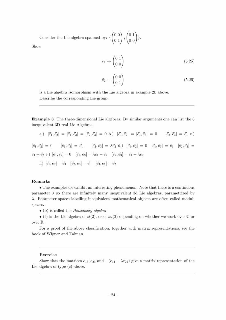
Consider the Lie algebra spanned by:
(0 0
0 1
),
(0 1
0 0
).
Show
~e1 7→
(0 1
0 0
)(5.25)
~e2 7→
(0 0
0 1
)(5.26)
is a Lie algebra isomorphism with the Lie algebra in example 2b above.
Describe the corresponding Lie group.
Example 3 The three-dimensional Lie algebras. By similar arguments one can list the 6
inequivalent 3D real Lie Algebras.
a.) [~e1, ~e2] = [~e1, ~e3] = [~e2, ~e3] = 0 b.) [~e1, ~e2] = [~e1, ~e3] = 0 [~e2, ~e3] = ~e1 c.)
[~e1, ~e2] = 0 [~e1, ~e3] = ~e1 [~e2, ~e3] = λ~e2 d.) [~e1, ~e2] = 0 [~e1, ~e3] = ~e1 [~e2, ~e3] =
~e1 + ~e2 e.) [~e1, ~e2] = 0 [~e1, ~e3] = λ~e1 − ~e2 [~e2, ~e3] = ~e1 + λ~e2
f.) [~e1, ~e2] = ~e3 [~e2, ~e3] = ~e1 [~e3, ~e1] = ~e2
Remarks
• The examples c,e exhibit an interesting phenomenon. Note that there is a continuous
parameter λ so there are infinitely many inequivalent 3d Lie algebras, parametrized by
λ. Parameter spaces labelling inequivalent mathematical objects are often called moduli
spaces.
• (b) is called the Heisenberg algebra
• (f) is the Lie algebra of sl(2), or of su(2) depending on whether we work over C or
over R.
For a proof of the above classification, together with matrix representations, see the
book of Wigner and Talman.
Exercise
Show that the matrices e13, e23 and −(e11 + λe22) give a matrix representation of the
Lie algebra of type (c) above.
– 24 –

5.3 Structure constants
Suppose we choose a basis ~ei for g as a vector space. Then there exist constants
[~ei, ~ej ] =∑k
fkij~ek (5.27) eq:structureconst
Definition fkij are called the structure constants of g wrt the basis ~ei.
Remark: It sometimes happens that Lie algebras are defined in terms of a special basis
together with relations (5.27). One must always be sure to check that such a presentation
in fact satisfies the Jacobi identity. There have been cases where someone proposes a new
Lie algebra, but the Jacobi identity fails (and hence no such Lie algebra exists).
Exercise Properties of structure constants
Show that
(a) f ijk = −f ikj(b) ∑
`
[f `ijf
m`k + f `jkf
m`i + f `kif
m`j
]= 0 ∀i, j, k,m (5.28)
In (a) there is in general no symmetry property relating i to j, k. (b) is equivalent to
the “Jacobi identity.”
Exercise
A symmetric bilinear form h : g× g→ k is said to be an invariant form if
h(Ad(X)Y, Z) + h(Y,Ad(X)Z) = 0 (5.29)
for all X,Y, Z.
Choosing a basis ei for g let hij = h(ei, ej) and define
fijk := hi`f`jk (5.30)
Show that if h is an invariant form then fijk is totally antisymmetric on all three
indices.
– 25 –

5.4 Representations of Lie algebras and Ado’s Theorem
In order to discuss the main theorem of this chapter, Lie’s theorem, we need a few definitions
and an auxiliary result, Ado’s theorem.
The space End(V ) of endomorphisms of a vector space V is a Lie algebra. Thus we
can define:
Definition: A representation of a Lie algebra g with representation space V is a Lie
algebra homomorphism
T : g→ End(V ) (5.31)
where End(V ) is the space of all linear transformations on V . We also say V is a g-module.
A matrix representation is a homomorphism T : g→Mn(k) for some n.
Put differently, we have a vector space V together with a multiplication
g× V → V
(X, v)→ X · v(5.32)
which is bilinear in X, v and such that
[X,Y ] · v = X · (Y · v)− Y · (X · v) (5.33)
Upon choosing a basis for V a g-module provides a matrix representation of g.
Two representations
Ti : g→ End(Vi) (5.34)
are said to be equivalent if there is an isomorphism S : V1 → V2 such that S−1T2(X)S =
T1(X) for all X ∈ g. If the representation defines an isomorphism of g with its image, i.e.
if kerT = 0, then the representation is said to be faithful.
Remarks
• Given any matrix representation of a Lie group G we automatically get a matrix
representation of the Lie algebra L(G): If X = ddtg(t)|0 ∈ g then
T (X) :=d
dtT (g(t))|0 (5.35) eq:diffgrp
Exercise
Show that (5.35) defines a Lie algebra representation T ([X,Y ]) = [T (X), T (Y )] by
using the BCH formula.
• Any Lie algebra has a canonical representation: V = g,
X ∈ g→ T (X) = Ad(X) ∈ End(g) (5.36)
where
Ad(X) : g→ g (5.37)
– 26 –

is the linear operator:
Ad(X)(Y ) := [X,Y ] (5.38) eq:adrep
This is called the adjoint representation.
Exercise The adjoint representation
a.) Show that (5.38) is a representation. To do this you must show:
[Ad(X), Ad(Y )] = Ad([X,Y ]) (5.39) eq:adrepii
b.) Show that the matrix elements of the adjoint representation wrt a basis Xi for g
are the given by the structure constants relative to that basis:
(Ad(Xi))kj = fkij (5.40) eq:strccnt
c.) Show that the kernel of the homomorphism X → Ad(X) is the center of the Lie
algebra:
Z(g) := X|Ad(X)Y = 0 ∀Y ∈ g (5.41)
Thus the adjoint representation is in general not a faithful representation of g.
d.) Suppose g is abelian. Describe the adjoint representation.
e.) Define the symmetric bilinear form
h(X,Y ) = TrgAd(X)Ad(Y ) (5.42)
Show that h(X,Y ) is an invariant bilinear form. This is known as the Cartan-Killing
metric, and is very important in determining the structure of semisimple Lie algebras.
Evidently, although every Lie algebra has a canonical representation - the adjoint
representation - this need not be a faithful representation.
Theorem[Ado’s Theorem]. Every finite dimensional Lie algebra has a faithful matrix
representation.
Proof : The proof is somewhat involved. See Jacobsen, Lie Algebras, p. 202. The main
idea is this: The kernel of the adjoint representation is the center Z(g). Therefore, if one
can find some representation V of g which is faithful on Z(g) then we can take a direct
sum with the adjoint representation: V ⊕ g to produce a faithful representation of g.
One begins by constructing a faithful representation of Z(g). If it is c-dimensional then
in a c + 1-dimensional vector space we choose a nilpotent operator N such that N c 6= 0.
Then Z(g) is represented by the commutative Lie algebra generated by N,N2, . . . , N c.
Indeed, we can choose any basis for Z(g) and map the basis elements to the powers of N .
Such a representation is faithful.
– 27 –

Thus we have produced a faithful representation, V ⊕ g , of Z(g) ⊕ (g/Z(g)). Next,
one needs to upgrade this into a representation of g itself. For the details, see Jacobsen. ♠************ should there be a discussion of irreps and schur’s lemma here? *************
6. Lie’s theorem
We have now seen how Lie algebras emerge from Lie groups. What about going the other
way, i.e. from Lie algebras to Lie groups?
Consider the case of matrix Lie algebras. If commutators are closed under some
property then exponentiating matrices will (locally) form a group, by the BCH formula.
For example, if A is anti-hermitian, A = −A†, then U = exp(A) is unitary:
UU † = (eA)(eA†) = eAe−A = 1 (6.1)
Conversely, consider the collection of unitary matrices of the form
U(N) = eA : A† = −A (6.2)
Claim: U(N) is locally closed under multiplication, i.e., it is closed as long as the BCH
formula converges. The main thing we must check is that if we write
eAeB = eC (6.3)
with C given by the BCH formula then C is antihermitian. Suppose A,B antihermitian
A† = −A,B† = −B. Then
[A,B]† = −[A,B] (6.4)
is antihermitian. Now, for the same reason, all the terms in the BCH series are antihermi-
tian since the expansion coefficients in the Taylor series expansion are real. Thus, just using
BCH we would be tempted to conclude that U(N) forms a group. However, we should
worry about three problems: The BCH series does not always converge, the exponential
map can fail to be surjective, and the exponential map is generally not 1-1. In fact, it turns
out that the exponential map for U(N) is actually surjective, and hence U(N) above is a
group after all, but we need extra information to reach this conclusion, and our discussion
would also fail for certain noncompact groups.
Thus, for the general case we are going to have to work harder.
The central theorem of the subject, Lie’s theorem, is the following: 5
Theorem:
a.) Every finite dimensional Lie algebra g arises from a unique (up to isomorphism)
connected and simply connected Lie group G.
b.) Under this correspondence, Lie group homomorphisms f : G1 → G2 are in 1 − 1
correspondence with Lie algebra homomorphisms µ : T1G1 → T1G2.
5We follow closely G. Segal’s elegant exposition in Lectures on Lie Groups and Lie Algebras, by R.
Carter, G. Segal, and I. MacDonald.
– 28 –

Remarks
• Locally isomorphic groups have the same Lie algebra, so we need to use the simply
connected cover to get a 1-1 correspondence.
•Warning: It follows from the theorem that if h is a sub Lie algebra of g = T1G then
there is a Lie group H such that h ∼= T1H, and moreover there is a group homomorphism
H → G. However, H need not be homomorphic to any topological subgroup of G. For
example, take G = SU(n), n > 2 and consider a U(1)× U(1) subgroup K of the maximal
torus, say
Diagλ, µ, (λµ)−1, 1, . . . , 1 λ, µ ∈ U(1) (6.5) eq:embedding
The group K has as Lie algebra the abelian Lie algebra R⊕R. The corresponding Lie
algebra homomorphism is
ν : (x, y)→ Diag2πix, 2πiy,−2πi(x+ y), 0, . . . , 0 (6.6)
Now, for h take the abelian Lie algebra R. Its corresponding connected and simply con-
nected Lie group is (R,+). Choose the homomorphism µ to be obtained by embedding Rinto R ⊕ R via 1 → (1, α) ∈ R ⊕ R. Considering R ⊕ R to be a subalgebra of L(SU(n))
using ν we have
µ : x→ Diag2πix, 2πiαx,−2πi(1 + α)x, 0, . . . , 0 (6.7)
The corresponding Lie group homomorphism (R,+)→ SU(n) guaranteed by the theorem
takes
x→ Diage2πix, e2πiαx, e−2πi(1+α)x, 1, . . . , 1 (6.8)
If α is rational, the image is a topological subgroup of SU(n). Now consider the case where
α is irrational. The image is a copy of the Lie group R embedded in SU(n), but this image
is not a topological subgroup of SU(n) since it is not a submanifold. Indeed, it densely
fills the U(1)× U(1) subgroup K.
• Lie’s theorem has an elegant and concise statement in the mathematical language
of categories. There is a category C1 whose objects are finite dimensional connected and
simply connected Lie groups, and whose morphisms are group homomorphisms. There is a
category C2 whose objects are finite dimensional Lie algebras, and whose morphisms are Lie
algebra homomorphisms. In categorical language, Lie’s theorem is simply the statement
that the functor G→ L(G) is an equivalence of the categories C1 and C2. Indeed, the point
of the theorem is to construct the functor L(G)→ G such that the composition of the two
functors is the identity. 6
Proof: Let us now sketch the proof of Lie’s theorem.
The hard part is showing that you can always exponentiate a finite dimensional Lie
algebra to form a Lie group.
6In general to prove an equivalence of categories one only needs a natural transformation of FG and GF
to the identity.
– 29 –

We use Ado’s theorem to assume that g ⊂ Mn(R) is a sub Lie-algebra of Mn(R) for
some n. 7
Our Lie group will be built by thinking about the (infinite dimensional!) space of
smooth paths
γ : [0, 1]→ g (6.9)
with γ(0) = γ(1) = 0. To such a path we can associate a group element gγ ∈ GL(n,R) by
the “holonomy”
gγ = P exp
∫ 1
0γ(t′)dt′ (6.10)
This can be defined using the path ordered product or as the solution gγ(1) to the first
order ODE:
d
dtgγ(t) = γ(t)gγ(t) (6.11) eq:dffqa
For bounded paths the path ordered exponential always converges, so gγ(1) is well-
defined.
Figure 1: A closed loop in the Lie algebra maps to an open path in GL(n,R). fig:looplie
We would like the set of elements gγ to form a subgroup. To do this we can add the
technical condition that all derivatives dn
dtnγ, n ≥ 1, vanish at t = 0, 1.
Define concatenation of paths:
γ1 ∗ γ2 =
2γ2(2t), 0 ≤ t ≤ 1
2
2γ1(2t− 1), 12 ≤ t ≤ 1
(6.12) eq:compone
The solution of (4.33) for this concatenation is
gγ1∗γ2(t) =
gγ2(2t), 0 ≤ t ≤ 1
2
gγ1(2t− 1)gγ2(1), 12 ≤ t ≤ 1
(6.13) eq:componea
and hence:
gγ1∗γ2 = gγ1gγ2 (6.14) eq:comptwo
7This can be dispensed with, but the proof is harder. See below.
– 30 –

Thus, group elements of the form gγ are closed under multiplication. Define G′ ⊂GL(n,R) to be the set of matrices gγ corresponding to paths of the above type. From
(6.14) we see that G′ is closed under group multiplication. Moreover, running γ backwards
gives the inverse element, so G′ is indeed a subgroup of GL(n,R). Unfortunately, G′ is not
quite the group we are after, because it might not be a topological subgroup of GL(n,R),
as the above example with irrational α shows. Therefore, we cannot conclude it is a Lie
group.
To take care of this we define P to be the space of all closed paths γ : [0, 1]→ g with
all derivatives vanishing at t = 0, 1:
P = γ : [0, 1]→ g|(d
dt
)nγ|t=0,1 = 0, n ≥ 0 (6.15) eq:curlype
This is an infinite-dimensional manifold. To compute the tangent space consider a
path of elements in P going through some γ∗(t). That is, a path of paths γ(s, t) with
γ(0, t) = γ∗(t). Differentiating a path of such paths gives
Tγ∗(t)P ∼= P (6.16) eq:curlypea
Moreover P has a multiplication γ1 ∗ γ2. But it is not quite an infinite-dimensional
Lie group - there is no identity or inverse. The natural identity would be the zero path
γ0(t) = 0, but γ0∗γ is only homotopic to γ. (P is in fact an infinite-dimensional homotopy-
Lie group.)
Now, equation (6.14) shows that P has a map to G′ preserving multiplication. The
group we are after is obtained from P by imposing an equivalence relation:
γ1 ∼ γ2 ⇔ gγ1 = gγ2 (6.17) eq:equivrel
We claim that G := P/ ∼ is a finite dimensional manifold, locally modeled on g, and
moreover it is a Lie group. We will compute its tangent space and Lie algebra in a moment.
Note that the quotient relation allows us to show that G really is a group. Moreover, it is
clearly connected and simply-connected, because we can shrink paths.
Thus, G will be a nice smooth Lie group, although its image G′ ⊂ GL(n,R) might be
very bad.
Now we would like to compute the tangent space to G, that is, the Lie algebra of G.
We work in the neighborhood of the zero path γ0(t) = 0 in P.
Recall that there is a neighborhood U of the identity in GL(n,R) so that log is well-
defined. By definition of the topology of P, there is an open neighborhood U of the zero
path in P obtained by considering those paths so that gγ(t) lies in U for all t and hence
loggγ(t) is well-defined. Define ηγ(t) for such a path by
gγ(t) = eηγ(t). (6.18) eq:defeta
At this point we only know that ηγ : [0, 1] → Mn(R). Note that although γ(t) are
closed paths in g, ηγ(t) in general will be an open path. We can take ηγ(0) = 0, but in
general gγ 6= 1 and in this case ηγ(1) cannot vanish.
– 31 –

Now we show that ηγ(t) is in fact valued in g, not just Mn(R). To do this, note that
γ(t) = (d
dtgγ(t))gγ(t)−1 =
eAd(ηγ(t)) − 1
Ad(ηγ(t))(ηγ(t)) (6.19) eq:diffleta
Now suppose γ(t) is scaled by ε. Then there a solution to (6.19) given by a power series in
ε: ηεγ(t) = εη1(t) + ε2η2(t) + · · · where we solve
η1 = γ(t)
η2 +1
2[η1, η1] = 0
η3 +1
2[η1, η2] +
1
2[η2, η1] +
1
6[η1, [η1, η1]] = 0
· · · = 0
(6.20)
By induction we see that ηγ(t) ∈ g for all t.
Now we remark that by (6.18) and the fact that exp is 1 − 1 in our neighborhood,
the equivalence relation (6.17) is the same as ηγ1(1) = ηγ2(1). The local neighborhood
K = π(U) of the identity in G is precisely
K ∼= η : [0, 1]→ g|η(0) = 0/ ∼ (6.21) eq:newlocnb
where
η1 ∼ η2 ⇔ η1(1) = η2(1) (6.22)
But this means that an equivalence class is uniquely parametrized by the element of g
given by the endpoint of the path. Moreover, the space P is trivially a Lie algebra: The
Lie bracket is just
[η1, η2](t) := [η1(t), η2(t)] (6.23) eq:liebrckt
and this Lie bracket descends to the equivalence relation. Thus, the space (6.21) is
isomorphic to g as a Lie algebra.
This establishes part (a) of the theorem.
To show part (b), first note that a homomorphism of Lie groups easily determines a
homomorphism of Lie algebras by considering one-parameter subgroups through 1. Now for
the converse, suppose we are given µ : g1 → g2. Using part (a) we can identify g1∼= T1G1
and g2∼= T1G2 where G1, G2 are connected and simply connected.
We would like to define f(g) by writing g = eX and taking
f(eX) := eµ(X) (6.24) eq:triy
Certainly, by BCH, if (6.24) makes sense then given that µ is a homomorphism of Lie
algebras, f is a homomorphism of Lie groups. The problem is that X need not exist, and
even if it does, it need not be unique. So, if eX = eX′
then it might not be true that
µ(X) = µ(X ′) and hence the attempt to define f by (6.24) in fact fails.
– 32 –

Instead we define f(g) as follows. To begin, we choose a path g(t), now in G1, not g1,
with g(0) = 1 and g(1) = g. We get a corresponding path in g1:
γ(t) := g(t)g−1(t). (6.25)
Let γ(t) := µ(γ(t)) be the corresponding path in g2. We can solve
d
dtg(t) = γ(t)g(t) (6.26)
with boundary condition g(0) = 1G2 , and attempt to define
f(g) := g(1). (6.27) eq:trydefii
Note that if we have two group elements g1, g2 then, as we have seen g1 ·g2 corresponds
to γ1 ∗ γ2, hence to γ1 ∗ γ2 hence to g1g2, so we do get a homomorphism.
The problem is, we need to show that f(g) in (6.27) is well-defined since we made a
choice of path g(t) to define it. It is exactly at this point we make use of the fact that G1
is simply connected. Suppose that g0(t), g1(t) are two paths with g0(1) = g1(1). Since G1
is simply connected we can write a homotopy g(s, t) between these two paths.
That is, there is a smooth map g(s, t) mapping I × I → G such that g(0, t) = g0(t),
g(1, t) = g1(t), g(s, 0) = 1 and g(s, 1) = g:
Then we define:
γ(s, t) :=∂
∂tg(s, t)g(s, t)−1
η(s, t) :=∂
∂sg(s, t)g(s, t)−1
(6.28) eq:twodervs
Note that these satisfy the Maurer-Cartan equation
∂
∂sγ − ∂
∂tη = [η, γ] (6.29) eq:mceq
An important point is that the converse also holds. Namely, (6.29) is the integrability
condition for the existence of a solution g(s, t) to (6.28) for a given γ, η.
Therefore, we apply the Lie algebra homomorphism µ to (6.29) to get
∂
∂sγ − ∂
∂tη = [η, γ] (6.30) eq:mceqa
– 33 –

and, using the converse result, this is the integrability condition for the existence of a
solution g(s, t) to
∂
∂tg(s, t) := γ(s, t)g(s, t)
∂
∂sg(s, t) := η(s, t)g(s, t)
(6.31) eq:twodervsa
Now, g(s, 1) = g is independent of s. Therefore η(s, 1) = 0. Therefore η(s, 1) = 0.
Therefore ∂∂s g(s, 1) = 0, so (6.27) is well-defined. ♠
Remarks
• As we mentioned, it is possible to avoid Ado’s theorem, and proceed directly from
g to the definition of the simply connected Lie group. To do this, we return to P, but
now we introduce a more subtle equivalence relation. Now we say that γ0 ∼ γ1 if there
exists a homotopy γ(s, t) of paths in P such that there is a partner η(s, t) satisfying the
Maurer-Cartan equation:∂
∂sγ − ∂
∂tη = [η, γ] (6.32)
for some η(s, t) ∈ g. Then we claim that P/ ∼:= G is the desired Lie group. The hard
part is to show that the Lie algebra of G is indeed g. To do this we solve
f(Adηγ(t))ηγ(t) = γ(t) (6.33)
and show that γ1 ∼ γ2 iff ηγ1(1) = ηγ2(1). Then
L(G) = η : [0, 1]→ g/ ∼ (6.34)
is isomorphic to g.
•We are really using here the theory of flat connections. The Maurer-Cartan equation
is the statement that the gauge field A = γdt+ ηds is a flat gauge field: F = dA+A2 = 0.
• One of the advantages of the above presentation is that it can be generalized to
infinite-dimensional Lie groups. See
J. Milnor, “Remarks On Infinite Dimensional Lie Groups,” In *Les Houches 1983,
Proceedings, Relativity, Groups and Topology, Ii*, 1007-1057
7. Lie Algebras for the Classical Groups
Now we can review the Lie algebras of some matrix groups, including the classical groups.
As we have seen, if G is a matrix group, that is, a Lie subgroup of GL(n, k) then the Lie
algebra associated to the Lie group G is:
L(G) ≡ A =d
dt
∣∣∣∣0
g(t) : g(t) = any curve g(t) with g(0) = 1 (7.1)
One way to think about Lie algebras related to the classical groups is as “infinitesimal
group elements.” Since Lie groups are manifolds we can consider a neighborhood of the
– 34 –

identity element 1G. In this neighborhood the manifold looks like a linear space, namely,
the tangent space T1G. We now want to get a better understanding of how the structure
of the group translates into an algebraic structure on T1G in the classical matrix groups.
For example, if G is a matrix group then matrices g ∈ G close to the identity can be
written as
g ∼= 1 + εA (7.2)
where ε is small. Thus infinitesimal group elements defines a matrix A in the Lie algebra.
Thus, for example, if A is anti-hermitian then 1 + εA is unitary to order ε2:
(1 + εA)(1 + εA)† = 1 +O(ε2) (7.3)
We will now list the relevant properties for the classical matrix groups. Our discussion
will parallel the survey we did of the matrix groups:
1. Definition and dimension.
2. Properties of the exponential map.
3. A natural choice of a Cartan subalgebra t ⊂ g. By definition, a Cartan subalgebra is
a maximal abelian subalgebra of g. It is of supreme importance in the theory of roots and
weights and representations. A Cartan subalgebra is the Lie algebra of a corresponding
Cartan torus.
7.1 A useful identity
The following identity is extremely useful: Given any n × n matrix A ∈ Mn(k), the
determinant and the trace may be related as follows:
det(exp(A)) = exp(TrA) (7.4) eq:trcelog
This is sometimes written
logdetC = TrlogC (7.5)
but the latter identity only makes sense when the log is well-defined.
We have already proven (7.4) above as an application of Jordan canonical form.
7.2 GL(n, k) and SL(n, k)
The Lie algebra of GL(n, k) is just the Lie algebra of all n× n matrices:
gl(n, k) ≡ L(GL(n, k)) = Mn(k) (7.6)
Let us check this by producing a one-parameter family. Let A ∈ Mn(k) and consider
g(t) := exp(tA). These matrices are all invertible, and
d
dt|t=0g(t) = A (7.7)
Thus we get the full Lie algebra of n× n matrices.
Again by deteA = exp(Tr(A)) we get
sl(n, k) ≡ L(SL(n, k)) = A ∈Mn(k) | trA = 0 (7.8)
– 35 –

We have a direct sum of Lie algebras:
gl(n, k) = k ⊕ sl(n, k) (7.9)
A natural choice of Cartan subalgebra is the subalgebra of diagonal matrices.
Remarks
• The exponential map is not onto for SL(n,R). Let us consider SL(2,R). If g = eA
then g lies on some one-parameter subgroup g(t) = etA. Any such can be conjugated into
a maximal abelian subgroup. From our classification of the conjugacy classes of SL(2,R)
it follows from hgh−1 = ehAh−1
that A can be conjugated to one of three possible forms:
A = x
(1 0
0 −1
)(7.10) eq:hyperbol
A = x
(0 −1
1 0
)(7.11) eq:elliptic
A = x
(0 1
0 0
)(7.12) eq:parabol
It is easy to check that the trace of eA for A conjugate to (7.10)(7.11)(7.12) is ≥ −2,
and the trace is = −2 only for g = −1 = exp[iπσ2]. In particular The parabolic conjugacy
classes with Tr(g) = −2 and the hyperbolic conjugacy classes with Tr(g) < −2 are not in
the image of the exponential map.
Exercise Structure constants for GL(n, k).
The Lie algebra has a natural basis given by the matrix units: ekj = The matrix with
zero entries except = 1 at (kj)th matrix element.
Calculate the structure constants
[eij , ekl] = δjkeil − δilekj (7.13)
Exercise Structure constants for sl(2,C) and sl(2,R)
Show that we may choose a basis
H =
(1 0
0 −1
)E+ =
(0 1
0 0
)E− =
(0 0
1 0
)(7.14) eq:spc
with structure constants
– 36 –

[E+, E−] = H
[H,E±] = ±2E±(7.15) eq:sltwo
We will see a lot more of this later.
Exercise The exponential map is onto for GL(n,C)
Show that
exp : gl(n,C)→ GL(n,C) (7.16) eq:expmapon
is surjective.
Answer : It suffices to check this statement for Jordan form. Therefore, try to write
λ+N , where N = e12 + e23 + · · · is a d× d Jordan block in the image of the exponential
map. Recall Nd = 0 but Nd−1 6= 0. Note that
exp[x1 + α1N + α2N2 + · · ·+ αd−1N
d−1] = (7.17)
= ex
(1 + α1N + (α2 +
1
2α2
1)N2 + · · ·+ (αd−1 + · · ·+ αd−11
(d− 1)!Nd−1
)(7.18)
and note that we can set ex = λ and then solve the upper-triangular system of equations
for the αi.
Exercise
a.) Show that matrices of the form(−x 0
0 −1/x
)(7.19)
for x > 0 are in SL(2,R), are in the image of the exponential map for SL(2,C), but not
in the image of the exponential map for SL(2,R).
b.) Show that (−1 1
0 −1
)(7.20)
is in SL(2,C), is in the image of the exponential map for GL(2,C), but not for SL(2,C).
– 37 –

7.3 O(n, k)
Suppose g(t) = etA is a family of orthogonal matrices. Then
g(t)g(t)tr = 1 (7.21) eq:orthone
since they are orthogonal for each t. Differentiate (7.21) wrt t to get:
d
dt|t=0e
tAetAtr
= A+Atr = 0 (7.22) eq:orthlie
and we can conclude from (7.22) that the Lie algebra of O(n, k) is the Lie algebra of
n× n skew matrices:
o(n, k) ≡ L(O(n, k)) = A ∈Mn(k) | Atr = −A (7.23)
Note that o(n, k) = so(n, k) because the groups O(n, k) and SO(n, k) have the same
neighborhood of the identity. In general locally isomorphic Lie groups have the same Lie
algebra.
Note that the exponential map is not one to one. For example:
exp[2π
(0 1
−1 0
)] = 1 (7.24)
Let us give a basis for the Lie algebra. Introduce the matrices:
Tij := eij − eji (7.25)
so that Tij = −Tji. Then Tij for 1 ≤ i < j ≤ n form a basis for o(n, k). We compute the
structure constants:
[Tij , Tkl] = δjkTil − δliTkj − δikTjl + δljTki (7.26) eq:soscs
N.B. Tij are elements of a Lie algebra - they are NOT matrix elements!
For o(2r, k), or o(2r + 1, k), a natural basis for a Cartan subalgebra is
T1,2, T3,4, . . . , T2r−1,2r. (7.27)
7.4 More general orthogonal groups
Recall that for any symmetric bilinear form D we can define an orthogonal group O(D).
If we choose a basis and represent D as a symmetric matrix Dij then O(D) becomes the
set of matrices with
gDgtr = D (7.28)
Following the procedure above we find the Lie algebra is the set of matrices A such that
AD +DAtr = 0. (7.29)
– 38 –

In particular, specializing to D = η = ((+1)p, (−1)q) we can rewrite this condition as:
(ηA)tr = −(ηA) (7.30)
Thus, the matrices are skew-symmetric after multiplication by η. Thus we could choose
a basis Tij ≡ ηTij , for o(p, q) where Tij are a basis for o(p + q). Thus a basis for the Lie
algebra is:
Tij = ηiieij − ηjjeji, 1 ≤ i < j ≤ n (7.31)
We can read off immediately the structure constants for o(p, q):
[Tij , Tkl] = ηjkTil − ηliTkj − ηikTjl + ηljTki (7.32) eq:soscsp
Again, we caution that the subcripts do not label matrix elements but elements in a
basis for the Lie algebra. In particular it is always true that:
Tij = −Tji. (7.33)
However, note that if ηii = ηjj then Tij is an antisymmetric matrix, but if ηii = −ηjj then
Tij is a symmetric matrix.
Exercise
Compute the structure constants for the Lorentz group
7.4.1 Lie algebra of SO∗(2n)
There is one other “real form” of SO(2n,C) given by matrices of the type:(A+ + iA− B+ + iB−−B+ + iB− A+ − iA−
)(7.34)
where A±, B± are real n× n matrices with
(A±)tr = −A± (B±)tr = ±B± (7.35)
For more discussion about this consult Gilmore, p.343.
7.5 U(n)
Proceeding to unitary matrices g(t) = etA is unitary if:
etA†etA = 1 (7.36)
Differentiating at t = 0 we conclude that:
A† = −A (7.37)
– 39 –

So:
u(n) = L(U(n)) = A ∈Mn(C) | A† = −Asu(n) = L(SU(n)) = A ∈ L(U(n)) : trA = 0
u(n) = R⊕ su(n)
(7.38)
A Cartan subalgebra is generated by matrices ieaa, a = 1, . . . n for u(n), but for su(n)
we need to have traceless matrices. One choice of basis is i(eaa − ea+1,a+1), 1 ≤ a ≤ n− 1.
Remarks
• Physicists usually separate out a factor of i =√−1 and write
U = eiH (7.39)
where H is hermitian.
•Note that the condition A† = −A is only preserved by multiplication of A by real
numbers so we must consider these as Lie algebras over R.
Exercise
Let us consider SU(2) in particular. Show that the Lie algebra can be thought of as
the real span of three anti-hermitian matrices (iJk), k = 1, 2, 3, with Jk Hermitian, such
that
[Ji, Jj ] = iεijkJk (7.40)
where εijk is the antisymmetric tensor on three indices. Take Ji = +12σi.
Note that the structure constants −εijk of this Lie algebra are real if we use the real
basis i2σ
i.
Exercise Relating o(4) and su(2)
We saw in the previous lecture that at the level of groups:
SO(4) =SU(2)× SU(2)
Z2(7.41) eq:sutwotwo
This must be reflected in the structure of the Lie algebras.
The Lie algebra version of (7.41) is that
o(4) ∼= su(2)⊕ su(2) (7.42)
Do this by defining
Aµν :=1
2εµνλρAλρ (7.43)
– 40 –

for any antisymmetric tensor Aµν = −Aνµ. In particular, for the generators of so(4) we
can define:
Tµν ≡1
2εµνλρTλρ (7.44)
Now form the “self-dual” and “anti-self-dual” combinations of generators:
A±µν =1
2[Tµν ± Tµν ] (7.45)
a.) Show that
A±µν = ±A±µν (7.46)
b.) Show that [A+, A−] = 0 and that
J1 → J+1 := A+
23 = A+14 =
1
2(T23 + T14)
J2 → J+2 := A+
31 = A+24 =
1
2(T31 + T24)
J3 → J+3 := A+
12 = −A+34 =
1
2(T12 + T34)
(7.47)
defines an isomorphism of the Lie subalgebra of the A+µν and su(2). Show that the corre-
sponding statement for the A−µν is
J1 → J−1 :=1
2(T23 − T14)
J2 → J−2 :=1
2(T31 − T24)
J3 → J−3 :=1
2(T12 − T34)
(7.48)
Exercise The ’t Hooft symbols
When working in Euclidean 4-dimensional physics the ’t Hooft symbol is often of great
use. This is defined by
α±,iµν :=1
2(±δiµδν4 ∓ δiνδµ4 + εiµν) (7.49) eq:thooft
where 1 ≤ µ, ν ≤ 4, 1 ≤ i ≤ 3 and it is understood that εiµν is zero unless 1 ≤ µ, ν ≤ 3.
a.) Show that in the previous exercise we can take:
J±,i =1
2α±,iµν Tµν (7.50)
b.) Show that if we regard α±,i as 4× 4 matrices with matrix elements α±,iµν then
[α±,i, α±,j ] = −εijkα±,k (7.51) eq:tfhti
– 41 –

[α±,i, α∓,j ] = 0 (7.52) eq:tfhtii
α±,i, α±,j = −1
2δij (7.53) eq:tfhtiia
See Belitsky, VanDoren, VanNieuwenhuizen, hep-th/0004186, for many more identities
of this nature. A closely related tensor are the so-called “’t Hooft symbols” ηaµν . Definitions
differ, but roughly η = 2α.
Exercise Spinor indices and ’t Hooft symbols
7.5.1 U(p, q)
The discussion here parallels that for O(p, q). Introduce η as before. Now a one-parameter
subgroup through 1 in U(p, q) satisfies
etA†ηetA = η (7.54)
for A ∈ u(p, q). Thus,
(ηA)† = −(ηA) (7.55)
and ηA is antihermitian.
Etc.
7.5.2 Lie algebra of SU∗(2n)
7.6 Sp(2n)
Following the same procedure as before we take a family of symplectic matrices g(t) = etA.
They must satisfy:
etAtrJetA = J (7.56)
Differentiating at t = 0 gives:
AtrJ + JA = 0 (7.57) eq:sympcond
Conversely, (7.57) and J2 = −1 imply:
−JeAtrJ = e−JAtrJ = e−A ⇒ eA
trJ = Je−A ⇒ eA ∈ Sp(2n, k) (7.58)
by pulling J to left and using (7.57) successively. so:
sp(2n, k) ≡ L(Sp(2n, k)) = A ∈M2n(k) | (JA)tr = +(JA) (7.59)
Now we can easily count the dimension of Sp(2n,R). We need only take a real sym-
metric 2n× 2n matrix and identify it with JA. Thus the dimension is:
– 42 –
dimRSp(2n,R) =1
22n(2n+ 1) (7.60) eq:dimen
in accord with a direct analysis at the group level.
Recall that the Cartan torus of USp(2n) is given by diagonal matrices of the form(Λ 0
0 Λ−1
)(7.61)
where Λ is a diagonal matrix of phases. The corresponding Cartan subalgebra is spanned
by
i(eaa − ea+n,a+n) a = 1, . . . , n (7.62)
Exercise
Define a basis mαβ for the Lie algebra from
Jmαβ = −(eαβ + eβα) (7.63)
i.e.
mαβ = J(eαβ + eβα) (7.64)
Show that
[mαβ,mγδ] = Jβγmαδ + Jαγmβδ + Jβδmαγ + Jαδmβγ (7.65)
One way to remember this is that the result must be symmetric on (α, β) as well as (γ, δ)
and antisymmetric on (α, β)↔ (γ, δ).
Exercise
It is also worthwhile to examine the condition (7.57) in terms of the block decomposi-
tion. Represent the matrix A in block form:
A =
(A11 A12
A21 A22
)(7.66)
Show that (7.57) implies:
Atr11 = −A22 (7.67)
Atr12 = A12 Atr21 = A21 (7.68)
Recall that if g ∈ Sp(2n) then gtr ∈ Sp(2n). Prove this using the Lie algebra.
– 43 –

Exercise su(1, 1) ∼= sl(2,R) ∼= sp(2,R)
a.) Show that a basis for the real Lie algebra su(1, 1) can be taken to be
E± =1
2(σ1 ∓ iσ3) (7.69)
H = σ2 (7.70)
and these satisfy the above standard commutation relations of sl(2,R).
b.) Note that sl(2,R) ∼= sp(2,R) trivially from the above characterization of block
diagonal form.
Exercise su(2) ∼= usp(2,R)
Exercise Solving the general quadratic Hamiltonian in quantum mechanics
Show that symplectic transformations allow us to solve the general quadratic Hamil-
tonian in quantum mechanics for a finite number of degrees of freedom:
Consider the general quadratic Hamiltonian for N degrees of freedom r = 1, . . . , N .
H = MrsPrPs +ArsPrXs +A∗rsXsPr +GrsXrXs (7.71) eq:ghen
where, after quantization [Pi, Qj ] = −iδij~, [Pi, Pj ] = [Xr, Xs] = 0. We restrict to
Hermitian Hamiltonians so that Mrs and Grs are real symmetric. Ars is an arbitrary
complex matrix.
a.) By adding a c-number we can assume that Ars is real.
b.) Write the Hamiltonian as
H =(Xr Pr
)J
(−Ars −Mrs
Grs Atrrs
)(Xs
Ps
)(7.72) eq:symphamil
and observe that it is of the form
H =(Xr Pr
)Jh
(Xs
Ps
)(7.73) eq:sntne
where h ∈ sp(2N,R).
– 44 –

Conclude that by a complex symplectic transformation(Xs
Ps
)→ g
(Xs
Ps
)(7.74)
we can bring h→ g−1hg into the Lie algebra of the Cartan torus. That is, we can bring it
to the form (iω 0
0 −iω
)(7.75)
where ω is diagonal and real. In this basis the Hamiltonian takes the form
H =
N∑i=1
ωiA†i , Ai (7.76)
c.) Finding the relevant transformation explicitly can be hard. The Hamiltonian can
be simplified and the problem can be reduced to the diagonalization of an N×N Hermitian
matrix as follows:
By a symplectic transformation X → TX,P → T tr,−1P we can bring Mrs to the form
δrs. Then, by conjugating with exp[i12SnmXnXm] we can make Ars antisymmetric. Thus
we can bring H to the form
H = PrPr +Ars(PrXs +XsPr) +GrsXrXs = (Pr +ArsXs)2 + (G+AtA)rsXrXs (7.77) eq:ghens
with Ars real antisymmetric. (This may be interpreted as charged particles in a con-
stant magnetic field in a quadratic potential.)
The Heisenberg equations of motion
−i~ ∂∂tO(t) = [H,O] (7.78)
become:
−i∂t
(Xr
Pr
)= K
(Xs
Ps
)(7.79) eq:heisenb
where
K = −2i
(A 1
−G A
)(7.80) eq:kay
1. K is in the symplectic Lie algebra sp(2N) and hence by a symplectic transformation
can be brought to the Cartan subalgebra:
U−1KU =
(ω 0
0 −ω
)(7.81) eq:cartfrm
– 45 –

where ω is N ×N diagonal. This is the transformation to creation/annihilation oper-
ators.
To find U note that eigenvectors of K are of the form(v1
v2
)(7.82)
with
L(E)v1 =E2
4v1 v2 = −(A− i
2E)v1 (7.83)
where L(E) = G + A2 − iEA. This is an Hermitian matrix and can be diagonalized with
eigenvalues fi(E). We then solve the quadratic equations fi(E) = E2/4.
8. Central extensions of Lie algebras and Lie algebra cohomology
The ideas here parallel those for central extensions of groups:
A central extension of a Lie algebra g by an abelian Lie algebra z is a Lie algebra g
such that we have an exact sequence of Lie algebras:
0→ z→ g→ g→ 0 (8.1)
with z mapping into the center of g. As a vector space (but not necessarily as a Lie algebra)
g = z⊕ g so we can denote elements by (z,X) and the Lie bracket has the form
[(z1, X1), (z2, X2)] = (c(X1, X2), [X1, X2]) (8.2)
where c : Λ2g→ z is known as a two-cocycle on the Lie algebra. That is c(X,Y ) is bilinear,
it satisfies
c(X,Y ) = −c(Y,X) (8.3) eq:twococyci
and the Jacobi relation requires
c([X1, X2], X3) + c([X3, X1], X2) + c([X2, X3], X1) = 0. (8.4) eq:twococycia
Two different cocycles can define isomorphic Lie algebras. If there is a linear function
f : g→ z such that
c(X,Y ) = bf (X,Y ) = f([X,Y ]) (8.5) eq:cobodn
then the cocycle is said to be trivial, and the central extension is isomorphic to z⊕ g
as a Lie algebra. Indeed,
X → (f(X), X) (8.6)
is an explicit Lie algebra homomorphism splitting the sequence. (Check!)
– 46 –

More generally, if two cocycles differ by a cocycle of the form bf then they define
isomorphic Lie algebras. Thus, again, classifying isomorphism classes of central extensions
is a cohomology problem, in this case, Lie algebra cohomology.
Remark: Suppose that G is a Lie group central extension of a Lie group G. Then
a 2-cochain c(X,Y ) defines a left-invariant 2-form on G, and a 2-cocycle defines a closed
left-invariant two-form ω on G. A central extension of the Lie group, defined by the group
cocycle f(g1, g2), also defines a corresponding 2-cocycle on the Lie algebra by
c(X1, X2) =1
2πi
d
dt1|0d
dt2|0log
[f(et1X1 , et2X2)
f(et2X2 , et1X1)
](8.7) eq:twoconscy
8.1 Example: The Heisenberg Lie algebra and the Lie group associated to a
symplectic vector space
In general, given any real vector space V and a skew bilinear form ω : V × V → R we can
view V as an abelian Lie algebra and use ω to define a central extension
0→ R→ heis(V, ω)→ V → 0 (8.8) eq:heisliealg
We simply use the cocycle c(v1, v2) = ω(v1, v2).
When ω is a symplectic form, i.e. ω is nondegenerate, then the corresponding Lie
algebra is called a Heisenberg Lie algebra.
The corresponding Lie group Heis(V, ω) is U(1)× V as a set with multiplication
(λ1, v1)(λ2, v2) = (λ1λ2eiω(v1,v2), v1 + v2) (8.9)
Let us return to the corollary (4.44) of the BCH formula:
eα1p+β1qeα2p+β2q = e−i2
(α1β2−α2β1)e(α1+α2)p+(β1+β2)q (8.10) eq:heisgroupiii
We can take V = R2 = (α, β) and we recognize
ω((α1, β1), (α2, β2)) = −1
2(α1β2 − α2β1) (8.11)
as the symplectic form in this case.
(Of course, we could take V = C2 and consider it as a 4-dimensional real vector space.
If we take α, β pure imaginary then the operators are unitary in the usual representation
on L2(R).)
Exercise
Check that eiω(v1,v2) is a 2-cocycle on the abelian group V .
– 47 –

Exercise
Referring to the exercise in section **** on the magnetic translation group
Show that the magnetic translation group generated by the Ui for all ai ∈ R is a
Heisenberg group, extending the abelian group of translations in the plane. Show that the
skew bilinear form is
ω(~a,~b) = −eB(~a×~b) (8.12) eq:skewfrm
8.2 Lie algebra cohomology
The notion of a two-cocycle above fits into a more general theory of Lie algebra cohomology.
So to put it into proper context let us briefly consider the topic more generally.
We consider the simplest case of central extensions by a one-dimensional abelian Lie
algebra k, z = k.
We define a complex
d : Λkg∗ → Λk+1g∗ (8.13) eq:lacoh
by taking as differential:
dω(X1, . . . , Xk+1) :=∑i<j
(−1)i+jω([Xi, Xj ], . . . Xi, . . . , Xj . . . ) (8.14) eq:extderi
The resulting differential (8.13) may also be expressed by identifying Λ∗g∗ = Λ∗[θa]
where θa are of degree 1 and a runs over a basis for the Lie algebra. We then define the
differential to be:
dθa := −1
2f abc θ
bθc (8.15) eq:lacohii
Exercise
Check that this is a differential, that is, that d2 = 0.
The cohomology of the complex (Λ∗g∗, d) is known as Lie algebra cohomology and
denoted H∗(g). Note that it can be formulated purely algebraically. The differential defined
by (8.14) or, equivalently, (8.15) is sometimes called the Chevalley-Eilenberg differential.
It is useful to translate this into the physicist’s language:
Suppose we have a Lie algebra g with basis Ta, a is an index running over the generators.
Let us introduce the Clifford algebra:
ca, ca′ = 0
ba, ba′ = 0
ca, ba′ = δaa′
(8.16) eq:ghosti
– 48 –

where ca, ba′ are referred to as ghosts and antighosts, respectively.
We can quantize the Clifford algebra by choosing a Clifford vacuum
ba′ |0〉 = 0 (8.17) eq:ghostii
and the resulting Hilbert space is spanned by |0〉, ca|0〉, ....The Hilbert space is graded by the “ghost number operator” N =
∑a c
aba, and we
have an isomorphism of the vector space of states of ghost number k with Λkg∗:
ω ↔ 1
k!ωa1···akc
a1 · · · cak |0〉 (8.18) eq:ghostiii
Under the isomorphism (8.18) the Chevalley-Eilenberg differential becomes what is
known as the BRST operator :
Q := −1
2f a1a2a3
ca2ca3ba1 (8.19) eq:ghostiv
The BRST cohomology is the cohomology of Q, and is graded by ghost number.
BRST cohomology enters physics in the quantization of theories with local gauge sym-
metry. For the moment let us note a very natural generalization. Suppose we have a
representation ρ of the Lie algebra g. We can then consider the complex
Λ∗g∗ ⊗ V (8.20)
and introduce a differential
Q = cata −1
2f a1a2a3
ca2ca3ba1 (8.21) eq:ghostv
where ta = ρ(Ta) are the representation matrices of the rep. V .
Geometrically, the cohomology H∗Q(Λ∗g∗ ⊗ V ) can be identified, for G compact and
connected, with the cohomology H∗DR(G;V) of a homogeneous vector bundle over the group
G.
Exercise
Check that Q2 = 0
Exercise
Compute the degree 2 Lie algebra cohomology of su(2) and show that it is trivial.
– 49 –

9. Left-invariant differential forms
We introduced the Lie algebra of a Lie group by thinking about the left-invariant vector
fields on the group. It is quite useful to think about the dual picture of left-invariant
differential forms:
Definition: A differential form ω ∈ Ω∗(G) is left invariant if
(Lg)∗(ω) = ω (9.1)
for all g ∈ G.
Suppose first that G = GL(n,F). Then we can construct an explicit basis of left-
invariant 1-forms as follows. The basis of one-forms dual to ξ(eij) is
Θi′j′ = (g−1)i′kdgkj′ (9.2) eq:dualbasis
One can check explicitly that Θi′j′ is a dual basis to ξ(eij) by computing the contrac-
tion:
ι(ξ(eij))(Θi′j′) = 〈Θi′j′ , ξ(eij)〉 = δii′δjj′ (9.3) eq:contraction
It is convenient to assemble the 1-forms Θij into a matrix of one-forms
Θ := Θijeij = g−1dg. (9.4) eq:maurercartan
Let us check the left-invariance directly in matrix notation:
(Lg0)∗(g−1dg) = (g0g)−1d(g0g) = g−1g−10 g0dg = g−1dg (9.5)
The matrix of 1-forms (9.4) is known as the Maurer-Cartan form. Note that, if X ∈gl(n,F) then we have
ι(ξ(X))(Θ) = X (9.6) eq:contr
Suppose now that G ⊂ GL(n,F) is a Lie subgroup. Under restriction to G the matrix
elements gij are not all independent, but satisfy polynomial relations. Nevertheless, we
can pull back the expression Θ = g−1dg to G. Formally, we should introduce the inclusion
map j : G → GL(n,F) and speak of ΘG = j∗(Θ). But to avoid cluttered notation we drop
this.
Now, for g ∈ G, the matrix of 1-forms will be valued in the lie algebra g of G considered
as a subalgebra of Matn(F). Indeed, if
γX(t) = g0etX (9.7)
is a curve through g0 whose directional derivative is ξ(X) then
γ∗X(g−1dg) = e−tXg−10 d(g0e
tX) = Xdt. (9.8)
– 50 –

This shows that
〈ξ(X),Θ〉 = X ∈ g (9.9)
In this way Θ = g−1dg defines the Maurer-Cartan forms on any Lie subgroup of a matrix
group.
Example G = SO(2) If
g =
(cos θ sin θ
− sin θ cos θ
)(9.10)
so
g−1dg =
(0 1
−1 0
)dθ (9.11)
so
〈 ∂∂θ, g−1dg〉 =
(0 1
−1 0
)(9.12)
10. The Maurer-Cartan equation
A very important property of the left-invariant 1-forms is the Maurer-Cartan equation.
Differentiating, using d2 = 0 and the Leibniz rule gives:
dΘ = −g−1dg ∧ g−1dg = −Θ ∧Θ (10.1) eq:derivmc
We thus have the Maurer-Cartan equation:
dΘ + Θ ∧Θ = 0 (10.2) eq:mcequations
Since in general the matrix product of two Lie algebra elements is not in the Lie
algebra, it might not be immediately obvious to the reader that Θ ∧ Θ is valued in g. To
make this obvious we proceed as follows:
It is often useful to choose a basis Ta for g. Then we can define structure constants:
[Ta, Tb] = f cab Tc (10.3)
Now, since g−1dg is valued in the Lie algebra g we can expand:
g−1dg = eaTa (10.4)
and this defines a system of 1-forms ea on G which span T ∗g (G) at any point g. Then we
compute
0 = deaTa + eaTa ∧ ebTb
= deaTa +1
2ea ∧ eb[Ta, Tb]
(10.5)
In terms of the structure constants we have:
dea +1
2f abc e
b ∧ ec = 0 (10.6) eq:structure
– 51 –

If follows from the above that the dual basis of vectorfields ea is precisely the system of
fundamental vector fields described above
ea = ξ(Ta) (10.7) eq:funda
Remarks:
• Although we have taken a rather concrete approach. The equations (10.6) and (10.7)
hold for all Lie groups. (Not all finite dimensional Lie groups are matrix groups. Heisenberg
groups give a counterexample. However, by the Peter-Weyl theorem, all compact Lie groups
are subgroups of some unitary group, and hence are matrix groups.)
• Later on, we will interpret this as a zero-fieldstrength condition for a pure gauge
field.
• Note that we can write:
Θ ∧Θ =1
2[Θ,Θ] (10.8)
where it is useful to introduce the notation
[α, β] := α ∧ β − (−1)pqβ ∧ α (10.9) eq:gradcomm
when α is a matrix-valued p-form and β is a matrix-valued q-form. Thus, the ordinary
commutator would read ΘΘ−ΘΘ = 0, but since we are discussing matrices whose elements
are in a graded algebra the natural notion of commutator is the “graded commutative”
(10.9).
• For future use in our discussion of connections on principal bundles, note that (10.2)
implies
Lξ(X)Θ = (dι(X) + ι(X)d)Θ = −ι(X)Θ2 = −Ad(X)(Θ) (10.10) eq:liederv
where in the last equality we consider Θ to be a Lie-algebra valued one-form, valued
in the adjoint representation.
Exercise
One way of defining the exterior derivative of a differential k-form field is via the
formula:
dω(X1, . . . , Xk+1) :=k+1∑i=1
(−1)i+1Xi
(ω(. . . , Xi, . . . )
)+∑i<j
(−1)i+jω([Xi, Xj ], . . . Xi, . . . , Xj . . . )
(10.11) eq:extderiv
where X means that entry is deleted.
a.) Using this formula, show that the Maurer-Cartan equation is equivalent to the fact
that the left-invariant vector fields form a closed Lie algebra.
– 52 –

b.) In particular, show that (10.6) is compatible with
[ea, eb] = +f cabec (10.12)
c.) Since left invariant forms are determined by their value at g = 1 we can identify
ΩkL(G) ∼= Λkg∗, as vector spaces. This gives us a new perspective on Lie algebra cohomology
defined above.
(Hint: If ω is left-invariant andXi are left-invariant then ω(X1, . . . , Xk) is left-invariant,
and hence constant.)
Exercise Right-invariance
a.) Show that
Θ = dgg−1 (10.13)
is a matrix of right-invariant 1-forms.
b.) Show that
dΘ− Θ ∧ Θ = 0 (10.14)
c.) Show that if we expand
Θ = ωaLTa (10.15)
Θ = ωaRTa (10.16)
then
ωaL = (Ad(g))abωbR (10.17)
so the bases of left- and right-invariant forms are related by the adjoint representation.
11. Examples
11.1 SU(2)
Introduce angular coordinates:
g = ei2σ3φe
i2σ2θe
i2σ3ψ
= ei12φσ3
(cos θ/2 sin θ/2
− sin θ/2 cos θ/2
)ei
12ψσ3
0 ≤ θ ≤ π, φ ∼ φ+ 2π ψ ∼ ψ + 4π
(11.1) eq:angl
Then
Θ = g−1dg =i
2σaea (11.2)
– 53 –
e1 = cosψ sin θdφ− sinψdθ
e2 = sinψ sin θdφ+ cosψdθ
e3 = dψ + cos θdφ
(11.3) eq:leftforms
which is conveniently written as
g−1dg =i
2σ3(dψ + cos θdφ) +
1
2
(0 1
0 0
)e−iψ(dθ + i sin θdφ)− 1
2
(0 0
1 0
)eiψ(dθ − i sin θdφ)
(11.4)
With the basis T a = i2σ
a the structure constants are f cab = −εabc, and one easily verifies
the Maurer-Cartan equations directly:
de3 = e1 ∧ e2 + cyclic (11.5) eq:sutmc
The dual basis of vector fields is
e3 =∂
∂ψ
e2 = cosψ∂
∂θ+
sinψ
sin θ
∂
∂φ− sinψcotθ
∂
∂ψ
e1 = − sinψ∂
∂θ+
cosψ
sin θ
∂
∂φ− cosψcotθ
∂
∂ψ
(11.6) eq:leftvfs
and one checks with an explicit computation that
[ea, eb] = −εabcec (11.7) eq:explicit
Remark: Note that dψ is not a globally well-defined form on SU(2), nor is cos θdφ.
However, the ea are globally well-defined. Similarly, the ea are globally well-defined vector
fields.
Exercise
It is often useful to introduce coordinates on C2:
z1 = rei(ψ+φ)/2 cos θ/2
z2 = rei(ψ−φ)/2 sin θ/2(11.8)
which satisfy |z1|2 + |z2|2 = r2. Setting r = 1 gives a coordinate system the covers SU(2)
(but degenerates at the poles).
Write out the forms in terms of these variables.
– 54 –

Exercise
Show that under g → g−1 we have
eaL(g) = −eaR(g−1) (11.9)
and that in coordinates this is φ↔ −ψ, θ → −θDeduce that
e1R = − cosφ sin θdψ + sinφdθ
e2R = sinφ sin θdψ + cosφdθ
e3R = dφ+ cos θdψ
(11.10) eq:rightforms
with dual basis of vector fields
eR3 =∂
∂φ
eR2 = cosφ∂
∂θ+
sinφ
sin θ
∂
∂ψ− sinφcotθ
∂
∂φ
eR1 = − sinφ∂
∂θ− cosφ
sin θ
∂
∂ψ+ cosφcotθ
∂
∂φ
(11.11) eq:leftvfsa
11.1.1 The Heisenberg group
An interesting example which is not a compact Lie group are the Heisenberg groups.
The three-dimensional Heisenberg group is the group of matrices
g =
1 x z
0 1 y
0 0 1
(11.12)
with x, y, z ∈ R. The multiplication law is
(x, y, z) · (x′, y′z′) = (x+ x′, y + y′, z + z′ + xy′) (11.13)
(note it is not abelian.)
An easy computation shows that
g−1dg =
0 dx dz − xdy0 0 dy
0 0 0
(11.14)
– 55 –

12. Metrics on Lie groups
A very natural class of metrics on Lie groups are those which are left or right invariant.
As with forms and vector fields (and indeed all tensors), invariant metrics are uniquely
determined by their value at g = 1, where they are bilinear forms on the Lie algebra. A
natural way to make such a metric is to choose a representation ρ of the Lie group and
define:
ds2 = Trρ(g−1dg)⊗ (g−1dg)
= Trρ(dgg−1)⊗ (dgg−1)
(12.1) eq:natmetric
Using equation (4.4)(??) above we see that this corresponds to the metric
(X1, X2) = Trρ(ρ(X1)ρ(X2)) (12.2) eq:natmetricii
on the Lie algebra.
Warning: While it is natural, the left-right invariant metric (12.1) might be zero. For
example, consider the group of upper triangular matrices with 1 on the diagonal. Similarly,
consider the Heisenberg group above. Also, for infinite-dimensional groups, the cyclicity of
the trace used in (12.1) might be invalid.
Metrics which are simultaneously left- and right- invariant correspond to Ad-invariant
metrics on the Lie algebra. Every Lie algebra has a canonical representation, namely, the
Adjoint representation. This defines the Ad-invariant Cartan-Killing metric:
gCK(X1, X2) := Trg(Ad(X1)Ad(X2)) (12.3) eq:cartkill
Example 1: O(n) has a basis for the Lie algebra Tij = eij − eji, 1 ≤ i, j ≤ n. Then
gCK(Tij , Tkl) = −2(n− 2)δi,kδj,l (12.4) eq:onck
Example 2: For SU(2), if we regard SU(2) = S3 as the unit sphere in Euclidean R4
then the metric is expressed in terms of the left-invariant forms is 1/2 of the metric in the
2-dimensional representation:
dΩ23 =
1
4
3∑a=1
ea ⊗ ea
=1
4
[(dψ + cos θdφ)2 + (dθ)2 + sin2 θ(dφ)2
]=
1
4
[(dψ)2 + (dθ)2 + (dφ)2 + 2 cos θdψdφ
] (12.5) eq:sumtrc
– 56 –

Exercise
Using the round metric of SU(2) compute the inner products of the left and right
invariant vector fields and show that
g(eLa , eLb ) = g(eRa , e
Rb ) = δab
g(eLa , eRb ) = Rab(ψ, θ, φ)
(12.6) eq:lrips
where Rab is the SO(3) rotation matrix associated with the Euler angles.
Exercise
Show that if we write the metric on a Lie algebra as
(Ta, Tb) := Iab (12.7)
then Ad-invariance is equivalent to:
f dac Idb = Iadf
dcb (12.8)
Exercise
Show that if we choose a basis Ta for g then the metric components of gCK are given
by
(gCK)ab = f dac f
cbd (12.9) eq:carkillii
Exercise
Compute the CK form for U(n), SU(n), USp(2n).
Exercise
Show that the volume of SU(N) in the metric
ds2 = −TrN [(g−1dg)⊗ (g−1dg)] (12.10) eq:metric
– 57 –

is
vol (SU(N)) =
√N
2π(2π)
12N(N+1) 1
1!2!3! · · · (N − 1)!(12.11)
Hint:
Consider SU(N)/SU(N − 1) = S2N−1 and relate the local coordinates of S2N−1 and
SU(N) via
g = 1 + iyNDiagε, . . . , ε, 1+∑i
(zieiN − zieNi) + · · · (12.12) eq:localcoord
at g = 1. (Here ε = −1/(N − 1). ). Here we are thinking of S2N−1 as the solutions to∑Ni=1 |zi|2 = 1 and zN = xN + iyN . In these coordinates, the group metric (12.10) becomes
ds2 = 2N−1∑i=1
[(dxi)2 + (dyi)2] +N
N − 1(dy)2 (12.13) eq:metrspher
Volumes of G and G/K for compact symmetric spaces (in the Killing metric) were
computed in A. Kojun and Y. Ichiro, “Volumes of compact symmetric spaces,” Tokyo J.
Math. 20 1997)p.87.
12.1 Simple Lie groups and the index of a representation
If we define a simple Lie algebra as one which has no nontrivial invariant subalgebras then
we have the following key result:
Exercise Uniqueness of the Cartan-Killing form
a.) Show that the Ad-invariant bilinear forms on a finite-dimensional simple Lie algebra
are unique up to a constant.
b.) Show that if Ta is an ON basis in the CK form, then the most general invariant
metric on a simple Lie group is
ds2 = Ω2dimG∑a=1
ea ⊗ ea (12.14)
where Ω2 is a constant.
Given the uniqueness of the CK form up to scale, for any representation ρ of g set
gρ(X1, X2) = Trρ(ρ(X1)ρ(X2)) = `(ρ)gCK(X1, X2) (12.15) eq:liemetric
where `(ρ) is a constant called the index of the representation. This is often useful to
have handy when working with instanton effects in gauge theory.
– 58 –
Example 1: For SU(2) we can easily compute the index of the irreducible represen-
tations by simply computing the norm-squared of J3. For the adjoint representation (spin
=1 ) we have
gCK(J3, J3) = 12 + 02 + (−1)2 = 2 (12.16) eq:cksut
and for spin j we have
gj(J3, J3) =
+j∑m=−j
m2 =
2j∑`=0
(−j + `)2 =1
3j(j + 1)(2j + 1) (12.17) eq:cksutii
and therefore,
f(j) =1
6j(j + 1)(2j + 1) (12.18)
Example 2 For SU(N), g = su(N) is the algebra of N ×N traceless antihermitian
matrices.
Tradj = 2NTrN (12.19) eq:indxemb
Remarks
• Tables of in the indexes of representations are given in books by Patera.
Exercise
Show that`(ρ1)
`(ρ2)=
dimρ1 · C2(ρ1)
dimρ2 · C2(ρ2)(12.20)
where C2(ρ) is the value of the Casimir in the representation ρ.
Exercise
Suppose that the decomposition of a tensor product of representations is given by
ρ1 ⊗ ρ2 =∑λ
Nλρλ (12.21)
Show that
`(ρ1)D(ρ2) + `(ρ2)D(ρ1) =∑λ
Nλ`(ρλ) (12.22) eq:relateindx
where D(ρ) is the dimension of ρ.
– 59 –

Exercise
Show that for a semisimple Lie algebra the degree two Lie algebra cohomology vanishes:
There are no nontrivial central extensions.
12.2 Metrics on abelian groups
In contrast to the simple groups, where the invariant metrics are unique up to an overall
constant, the metrics on abelian groups are far from unique. Indeed, the torus U(1)n has
a moduli space of invariant metrics GL(n,R)/O(n).
12.3 Geodesics
Geodesics through the origin are of the form γ(t) = exp[tX] for X ∈ g.
********** EXPLAIN WHY **************
12.4 Compact and noncompact real forms: The signature of the CK metric
For a good discussion on this topic see Gilmore’s book.
By the KAN decomposition (Gram-Schmidt decomposition) we see that every con-
nected Lie group is (topologically) a product of its maximal compact subgroup and a
Euclidean space.
A general result identifies the compact subalgebra with the negative definite generators
and the noncompact generators with the positive definite subspace.
Key example: Compact generator
X =
(0 1
−1 0
)⊕ 0⊕ 0⊕ · · · (12.23)
This is compact in the sense that its 1-parameter subgroup forms a compact orbit:
exp[tX] =
(cos t sin t
− sin t cos t
)⊕ 1⊕ 1⊕ · · · (12.24)
Note that:
Tr(X)2 = −2 (12.25)
while a noncompact generator
X =
(0 1
1 0
)⊕ 0⊕ 0⊕ · · · (12.26)
has
exp[tX] =
(cosh t sinh t
sinh t cosh t
)⊕ 1⊕ 1⊕ · · · (12.27)
and
Tr(X)2 = +2 (12.28)
– 60 –

12.5 Example: SL(2, R)
The Lie algebra sl(2,R) is the Lie algebra of traces 2× 2 real matrices.
One natural basis of the Lie algebra has commutation relations:
[K0,K±] = ±K±, [K+,K−] = −2K0 . (12.29) eq:sucom
In the 2-dimensional representation we could take, for example:
K0 =1
2
(1 0
0 −1
)K+ =
(0 1
0 0
)K− =
(0 0
−1 0
)(12.30)
Maurer-Cartan forms:
U := eC+K+eC0K0eC−K−
dUU−1 = e−C0dC−K− + (dC0 − 2e−C0C+dC−)K0 + (dC+ + e−C0C2+dC− − C+dC0)K+
U−1dU = dC+e−C0K+ + (dC0 − 2C−e
−C0dC+)K0 + (dC− − C−dC0 + C2−e−C0dC+)K−
(12.31) eq:mcforms
The Killing metric is:
(aK0 + bK+ + cK−, aK0 + bK+ + cK−) = 2(a2 − 4bc) (12.32)
Note that this is a Lorentzian signature metric.
Casimir:
4K20 − 2(K+K− +K−K+) (12.33)
The compact generator is K+ +K− and the KAN decomposition is:
SO(2)
(λ
λ−1
)(1 x
0 1
)(12.34)
Exercise
a.) Compute the Maurer-Cartan forms in the global coordinates of the KAN decom-
position.
b.) Suppose we write the Gauss decomposition:
g =
(1 0
χ 0
)(eφ 0
0 e−φ
)(1 ψ
0 1
)(12.35)
(warning: These are not globally valid coordinates on SL(2,R).) Show that
Tr(g−1dg)3 = 2e2φdφ ∧ dψ ∧ dχ (12.36)
– 61 –
References:
1. A comprehensive reference on the geometry (but not the topology) of Lie groups
is Helgason, Differential Geometry, Lie Groups, and Symmetric Spaces, Academic Press,
1978.
2. A less systematic, but more readable account for physicists is R. Gilmore, Lie
Groups, Lie Algebras, and Some of Their Applications, John Wiley, 1974.
13. Some Remarks on Infinite Dimensional Lie Algebras
13.1 Generalities
The study of infinite dimensional Lie algebras and their representations is an active subject
in modern mathematical physics. Infinite dimensional Lie algebras arise in conformal
field theory, string theory, gauge theory of elementary particles, and gravitational theory
classical and quantum mechanical. They have also play a role in some field theoretical
applications of condensed matter physics such as the quantum Hall effect, and the Kondo
problem.
***************
Banach Lie groups. Comments from Milnor.
***************
13.2 Groups of operators on Hilbert space
A very important infinite-dimensional group is the group U(H) of unitary operators on
Hilbert space. The topology of this group depends strongly on how we define the group
precisely. The inductive limit limn→∞ U(n) has lots of topology (it is a classifying space
for K1).
On the other hand, there is a very deep and remarkable theorem, known as Kuiper’s
theorem U(H) which states that in the norm topology U(H) is contractible!
13.3 Gauge Groups
For another set of examples, consider a Lie group G, and a manifold M . The space of all
smooth maps M → G forms an infinite-dimensional group with Lie algebra the space of
all maps M → g. Except for the case where M is one-dimensional, very little is known
about these groups. The one-dimensional case is of central importance in string theory
and low-dimensional field theory.
13.3.1 Loop algebras
Suppose g is a finite dimensional simple Lie algebra. We can associate to it an infinite
dimensional Lie algebra whose elements are maps
f : S1 → g (13.1)
We will be vague about the precise class of maps - it should be some completion of the
space of Laurent polynomials in z = eiθ. The set of all such maps is itself a Lie algebra for
– 62 –

we can define
[f1, f2](z) := [f1(z), f2(z)] (13.2)
This infinite dimensional Lie algebra is known as the loop algebra Lg.
It is often useful to choose a basis T a for g, for this induces an obvious basis for Lg:
T an := T azn (13.3)
with commutation relations
[T an , Tbm] = fabc T
cn+m (13.4)
Loop algebras admit a very interesting central extension: 8
0→ R→ Lg→ Lg→ 0 (13.5)
Elements of Lg are pairs (f, ξ) where f is a map, and ξ ∈ C. The bracket of the central
extension is
[(f1, ξ1), (f2, ξ2)] := ([f1, f2], ω(f1, f2)) (13.6)
where
ω(f1, f2) :=1
2πi
∮(f ′1(z), f2(z))gdz (13.7)
where in the integral we use an ad-invariant bilinear form (·, ·)g, such as the Cartan-Killing
form on g. (Recall that for G simple all such forms are the same up to scale, consistent
with the uniqueness of the central extension.)
Again, it is useful to write this out in terms of a basis. Using the bilinear form on g
we define
(T a, T b)g = gab (13.8)
and we define K := (0, 1) ∈ Lg. Then
[T an , Tbm] = fabc T
cn+m + ngabδn+m,0K
[K,T an ] = 0(13.9) eq:kmalg
This is the way the algebras are often written in the physics literature.
13.4 Diffeomorphism Groups
A nice example is given by the space of vector fields on a manifold and the related group
of diffeomorphisms of a manifold.
Already, the simplest special case is highly nontrivial. Consider the group diffeomor-
phisms of the circle.
A natural basis of vector fields on the circle is given by Fourier decomposition:
`n = ieinθd
dθ(13.10)
8It is an easy result that, up to isomorphism, this is the unique nontrivial central extension when g is
simple.
– 63 –

They satisfy the Lie algebra:
[`n, `m] = (n−m)`n+m (13.11)
One can show that there is a one-dimensional cohomology space and a representative
cocycle is
ω(`n, `m) = δn+m,0n3 (13.12) eq:repcocycl
Note this is cohomologous to
ω(`n, `m) = δn+m,0(n3 − n) (13.13) eq:repcocycla
The unique central extension of the Lie algebra of vector fields on S1 is known as the
Virasoro algebra.
The Virasoro algebra can be defined in terms of a basis Ln, n ∈ Z and a central element
c, with structure constants:
[c, c] = 0
[c, Ln] = 0
[Ln, Lm] = (n−m)Ln+m +c
12(n3 − n)δn+m,0
(13.14) eq:virasoro
The normalization of the central element c is convenient in physical applications. The
choice of cocycle is made so that the Lie algebra generated by L±1, L0 forms a copy of sl(2)
and is not extended.
Exercise
a.) Check the Jacobi relations of the Virasoro algebra.
b.) Show that ω(`n, `m) = nδn+m,0 is a coboundary.
c.) Show that the Lie algebra cohomology of the conformal group is one-dimensional
and hence show that the above is the most general central extension.
13.4.1 Gravity in 1+1 dimensions
Consider quantum gravity in 1 + 1 dimensions. If space is compact and connected it must
be S1, we are therefore interested in invariant states under G = Diff+(S1). A natural
basis for the corresponding (complexified) Lie algebra is given by `n = einθ ddθ , n ∈ Z.
Actually, because this is an infinite-dimensional group we should allow for anomalies and
work with a central extension. The corresponding Lie algebra is the Virasoro algebra given
above. Let us see how the central extension comes about physically.
Let us consider the BRST operator. We introduce (diffeomorphism) ghosts and antighosts
cn, bn, n ∈ Z with cn, bm = δn+m,0.
– 64 –

Because we are working with an infinite-dimensional Clifford algebra there are many
inequivalent quantizations. The one relevant to radial quantization in the complex plane
of string theory is 9
cn|0〉 = 0 n > 1
bn|0〉 = 0 n > −2(13.15) eq:ghostvac
The idea here is that the “Dirac sea” is filled by c2 ∧ c3 ∧ c4 ∧ · · · . For this reason,
elements of the ghost Hilbert space are referred to as “semi-infinite differential forms” in
the math literature.
Following the formula (8.19) above we have in this case:
Qghost = −1
2
∑m,n∈Z
(m− n) : c−mc−nbm+n : (13.16) eq:virq
The normal ordering is necessary so that Q has a well-defined action on the ghost
Hilbert space.
Now one finds a big surprise: Q2 6= 0 due to the need to regularize the infinite sums!
Using ζ-function regularization one computes
Q2ghost =
∑m,n
(m− 13m3)
12δm+n,0cmcn (13.17) eq:virqiii
If we consider the Lie algebra cohomology in a nontrivial Virasoro module with central
charge ρ(c) then the BRST operator is:
Q =∑
cnρ(Ln)− 1
2
∑m,n∈Z
(m− n) : c−mc−nbm+n : −ac0 (13.18) eq:virqiv
where we have allowed for a normal-ordering shift ρ(L0)→ ρ(L0)− a. Then
Q2 =1
2
∑m,n∈Z
[[ρ(Ln), ρ(Lm)]− (n−m)ρ(Ln+m) +
((1 + 12a)m− 13m3)
6δm+n,0
]cmcn
(13.19) eq:virqiiia
so we get Q2 = 0 for a = 1 and ρ(c) = 26.
In the worldsheet approach to string theory we work with 1 + 1 dimensional quantum
gravity coupled to matter and this is one way of understanding the restriction to matter
with c = 26. Only in this case is there a well-defined spectrum of string states from BRST
cohomology.
9In general, a primary field of dimension ∆ has an expansion Φ =∑n Φnz
−n−∆ and hence Φn|0〉 = 0
for n > −∆, so that limz→0 Φ(z)|0〉 is well-defined. The ghost field c(z) has ∆ = −1 and the antighost b(z)
has dimension ∆ = +2.
– 65 –

13.4.2 The exponential map for Diff(S1)
• For Diff(S1) the Exp map is neither 1-1 nor onto, even in an arbitrarily small neigh-
borhood of the origin!
• For V irC there is no corresponding Lie group.
For a discussion of (1) above see Pressley+Segal, Loop Groups, Sections 3.3.1 and the
article by Milnor. Briefly, to show exp is not 1− 1 consider rotation R2π/n. Consider the
centralizer Z(R2π/n). This consists of diffeomorhisms which are periodic in the sense that
φ(θ + 2π/n) = φ(θ) + 2π/nmod2π. Now for any φ in the centralizer, φSO(2)φ−1 is a one
parameter subgroup of Diff(S1) consisting of elements φRθφ−1|θ ∈ R. However, R2π/n
lies on all these one-parameter subgroups! Thus, the exponential map is not 1-1. Note
that we can make n arbitrarily large, so this failure of injectivity holds arbitrarily close to
the identity.
Regarding (2) consider the following diffeomorphism
f(θ) = θ + π/n+ ε sin2(nθ) (13.20)
where 0 < ε < 1/n. One can prove that this diffeomorphism has precisely one periodic
orbit of length 2n: 0 → π/n → 2π/n → · · · → 2π(n − 1)/n → 0. Indeed, if 0 < θ0 < π/n
then defining θj+1 = f(θj) one can check with a little calculus that
θ0 < θ1 − π/n < θ2 − 2π/n < · · · < π/n (13.21)
so no θj is ever equal to θ0 modulo 2π. Thus, our diffeomorphism has precisely one periodic
orbit, and it is of length 2n. It is remarkable that it has only one orbit with an even number
of elements in the orbit. Why?
Consider a diffeomorphism F of any manifold. It is useful to compare the periodic
orbits of F with those of F F . If F has an odd periodic orbit then, F F has the same
odd periodic orbit, essentially because the order of the orbit and 2 are relatively prime.
(Draw the case of n = 3, 5.) On the other hand, if F has an even periodic orbit of order
n = 2m, then the periodic orbits of F F split up into two distinct periodic orbits of length
m. (Check the cases n = 4, 6.)
Now, we apply this remark to note that f(θ) above cannot be of the form F F for any
diffeomorphism F , since the number of periodic orbits of even period must be even, but
f(θ) has a single periodic orbit of even period. But this in turn means that f(θ) cannot
be on any one-parameter subgroup Ft(θ) since if we had Ft∗(θ) = f(θ) then we would have
had f = F F with F = F 12t∗
.
For a discussion of point (2) above see section 3.3.2 of Pressley-Segal. ♣Need to explain
why. Helpful
remarks in
Graeme’s email
from November 19,
2009 on this. ♣
– 66 –


![Chapter 7 Lie Groups, Lie Algebras and the Exponential Mapcis610/cis61005sl8.pdf · Lie Groups, Lie Algebras and the Exponential Map 7.1 Lie Groups and Lie Algebras In Gallier [?],](https://img.pdfslide.net/doc/110x75/5f0c1a337e708231d433c07b/chapter-7-lie-groups-lie-algebras-and-the-exponential-map-cis610-lie-groups.jpg)