Lecture 8Lecture 8

Numerical Analysis

Numerical Analysis

Solution of Non-Linear Equations

Solution of Non-Linear Equations

Chapter 2Chapter 2

IntroductionBisection MethodRegula-Falsi MethodMethod of iterationNewton - Raphson MethodSecant MethodMuller’s MethodGraeffe’s Root Squaring Method

IntroductionBisection MethodRegula-Falsi MethodMethod of iterationNewton - Raphson MethodSecant MethodMuller’s MethodGraeffe’s Root Squaring Method

Muller’s MethodMuller’s Method

Suppose, Suppose,

be any three distinct be any three distinct approximations to a root approximations to a root

of of ff ( (xx) = 0. ) = 0.

2 1, ,i i ix x x

2 2 1 1( ) , ( )i i i if x f f x f

( ) .i if x f

Noting that any three distinct Noting that any three distinct points in the (points in the (xx, , yy)-plane )-plane uniquely, determine a uniquely, determine a polynomial of second degree. polynomial of second degree.

A general polynomial of A general polynomial of second degree is given by second degree is given by

2( )f x ax bx c

Suppose, it passes through the pointsSuppose, it passes through the points

2 2 1 1( , ), ( , ), ( , )i i i i i ix f x f x f

22 2 2i i iax bx c f

21 1 1i i iax bx c f

2i i iax bx c f

then the following equations will then the following equations will be satisfiedbe satisfied

Fig: Quadratic polynomial.

Eliminating Eliminating a, b, ca, b, c, we obtain, we obtain

2

22 2 2

21 1 1

2

1

10

1

1

i i i

i i i

i i i

x x f

x x f

x x f

x x f

which can be written aswhich can be written as1

22 1

21

1 2 1

( )( )

( )

( )( )

( )( )

i ii

i i

i ii

i i i i

x x x xf f

x x

x x x xf

x x x x

2 1

2 1

( )( )

( )( )i i

ii i i i

x x x xf

x x x x

The above equation can be written asThe above equation can be written as

1

1 1 2

,

,i

i i i

i i i

h x x

h x x

h x x

That was a second degree That was a second degree polynomial. polynomial.

Now, introducing the notationNow, introducing the notation

The above equation can be written asThe above equation can be written as

21 1

11

1

( )

( )

( )

( )( )

ii

i i i

i ii

i i

h h hf f

h h h

h h h hf

h h

1

1

( )( )

( )i i i

ii i i

h h h h hf

h h h

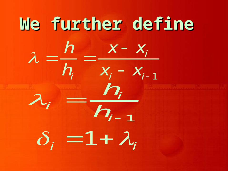
We further defineWe further define

1

i

i i i

x xh

h x x

1

ii

i

h

h

1i i

With these substitution we With these substitution we get a simplified Equation asget a simplified Equation as

22

11

1

1[ ( 1)

( 1 )

( 1 ) ]

i ii

i i i i

i i i

f f

f

f

Or

2 2 12 1

2 22 1

1

( )

[

( )]

i i i i i i i i

i i i i

i i i i i

f f f f

f f

f f

To compute set To compute set ff = 0 = 0, we obtain, we obtain

wherewhere

A direct solution will lead to loss of A direct solution will lead to loss of accuracy and therefore to obtain accuracy and therefore to obtain max accuracy we rewrite as:max accuracy we rewrite as:

,2

2 1( ) 0i i i i i i i i if f f g f

2 22 1 ( )i i i i i i i ig f f f

2 12( ) 0i i ii i i i i i

f gf f f

so that, so that,

oror

Here, the positive sign must be so Here, the positive sign must be so chosen that the denominator becomes chosen that the denominator becomes largest in magnitude.largest in magnitude.

2 1/ 22 1[ 4 ( )]1

2i i i i i i i i i i

i i

g g f f f f

f

2 1/ 22 1

2

[ 4 ( )]i i

i i i i i i i i i i

f

g g f f f f

we can get a better approximation to the root, by using

1i i ix x h

ExampleExampleDo two iterations of Muller’s Do two iterations of Muller’s method to solve method to solve

starting withstarting with

0 2 10.5, 0, 1x x x

3 3 1 0x x

SolutionSolution3

0 0( ) (0.5) 3(0.5) 1 0.375f x f 3

1 1( ) (1) 3(1) 1 1f x f

2 2( ) 0 3 0 1 1f x f

0 0.375c f 1 1 0 0.5h x x

2 0 2 0.5h x x

2 1 1 2 0 1 2

1 2 1 2

( )

( )

h f h h f h fa

h h h h

(0.5)( 1) ( 0.375) (0.5)

1.50.25

21 0 1

1

2f f ah

bh

0 2

2

4

cx x

b b ac

2( 0.375)

0.52 4 4(1.5)(0.375)

0.750.5 0.33333 0.5

2 4 2.25

2 0 10, 0.33333, 0.5x x x 1 1 0 2 0 20.16667, 0.33333h x x h x x

0

30 0

(0.33333)

3 1 0.037046

c f f

x x

Take

= 0.8333

31 1 13 1 0.375f x x

32 2 23 1 1f x x

2 1 1 2 0 1 2

1 2 1 2

( ) 0.023148

( ) 0.027778

h f h h f h fa

h h h h

21 0 1

1

2.6f f ah

bh

0 2

0

2

40.074092

0.3333335.2236

0.3475 0.33333

cx x

b b ac

x

For third iteration take,

2 0 10.333333, 0.3475, 0.5x x x

Graeffe’s Root Squaring Method

Graeffe’s Root Squaring Method

GRAEFFE’S ROOT SQUARING GRAEFFE’S ROOT SQUARING METHOD is particularly METHOD is particularly attractive for finding all the roots attractive for finding all the roots of a polynomial equation. of a polynomial equation.

Consider a polynomial of third Consider a polynomial of third degreedegree

2 30 1 2 3( )f x a a x a x a x

2 30 1 2 3( )f x a a x a x a x

2 3 2 23 2 1 3

2 21 0 2 0

( ) ( ) ( 2 )

( 2 )

f x f x a t a a a t

a a a t a

2 30 1 2 3( )f x a a x a x a x

2 6 2 43 2 1 3

2 2 21 0 2 0

( ) ( ) ( 2 )

( 2 )

f x f x a x a a a x

a a a x a

The roots of this equation are The roots of this equation are squares or 2squares or 2ii ((ii = 1), powers of the = 1), powers of the original roots. Here original roots. Here ii = 1 indicates = 1 indicates that squaring is done once.that squaring is done once.

The same equation can again be The same equation can again be squared and this squaring process squared and this squaring process is repeated as many times as is repeated as many times as required. After each squaring, the required. After each squaring, the coefficients become large and coefficients become large and overflow is possible as overflow is possible as ii increases. increases.

Suppose, we have squared the Suppose, we have squared the given polynomial ‘given polynomial ‘i’i’ times, then times, then we can estimate the value of the we can estimate the value of the roots by evaluating roots by evaluating 22ii root of root of

where where nn is the degree of the is the degree of the given polynomial. given polynomial.

1

, 1, 2, ,i

i

ai n

a

The proper sign of each The proper sign of each root can be determined root can be determined by recalling the original by recalling the original equation. This method equation. This method fails, when the roots of fails, when the roots of the given polynomial are the given polynomial are repeated. repeated.

Example Example Using Graeffe root Using Graeffe root squaring method, find all squaring method, find all the roots of the equationthe roots of the equation

3 26 11 6 0x x x

SolutionSolution

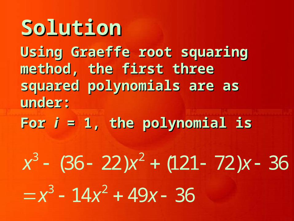
Using Graeffe root squaring Using Graeffe root squaring method, the first three squared method, the first three squared polynomials are as under:polynomials are as under:

For For ii = 1, the polynomial is = 1, the polynomial is

3 2

3 2

(36 22) (121 72) 36

14 49 36

x x x

x x x

For i = 2, the polynomial is

3 2

3 2

(196 98) (2401 1008) 1296

98 1393 1296

x x x

x x x

For i = 3, the polynomial is3 2

3 2

(9604 2786) (1940449 254016) 1679616

6818 16864333 1679616

x x x

x x x

The roots of polynomial are

Similarly, the roots of polynomial (2) are

36 49 140.85714, 1.8708, 3.7417

49 14 1

44 41296 1393 98

0.9821, 1.9417, 3.14641393 98 1

Still better estimates of the roots Still better estimates of the roots obtained from polynomial (3) areobtained from polynomial (3) are

The exact values of the The exact values of the roots of the given roots of the given polynomial are 1, 2 and 3.polynomial are 1, 2 and 3.

88 81679616 1686433 6818

0.99949, 1.99143, 3.01441686433 6818 1

Lecture 8Lecture 8

Numerical Analysis

Numerical Analysis

Revision ExampleRevision ExampleObtain the Newton-Raphson Obtain the Newton-Raphson extended formulaextended formula

for finding the root of the for finding the root of the equation equation ff ( (xx) = 0. ) = 0.

20 0

1 0 030 0

( ) [ ( )]1( )

( ) 2 [ ( )]

f x f xx x f x

f x f x

Solution Solution Expanding Expanding ff ( (xx) by Taylor’s series, in the ) by Taylor’s series, in the neighborhood of neighborhood of xx00, we obtain after , we obtain after retaining the first order term onlyretaining the first order term only

Which givesWhich gives

This is the first approximation to the root. This is the first approximation to the root. Therefore,Therefore,

0 0 00 ( ) ( ) ( ) ( )f x f x x x f x

00

0

( )

( )

f xx x

f x

01 0

0

( )

( )

f xx x

f x

Expanding Expanding ff ( (xx) by Taylor’s ) by Taylor’s series and retaining up to series and retaining up to second order term,second order term,

Therefore,Therefore,

0 0 0

20

0

0 ( ) ( ) ( ) ( )

( )( )

2

f x f x x x f x

x xf x

1 0 1 0 0

21 0

0

( ) ( ) ( ) ( )

( )( ) 0

2

f x f x x x f x

x xf x

This can also be written as This can also be written as

Thus, the Newton-Raphson extended Thus, the Newton-Raphson extended formula is given byformula is given by

This is also known as Chebyshev’s formula This is also known as Chebyshev’s formula of third orderof third order

20

0 1 0 0 020

[ ( )]1( ) ( ) ( ) ( ) 0

2 [ ( )]

f xf x x x f x f x

f x

20 0

1 0 030 0

( ) [ ( )]1( )

( ) 2 [ ( )]

f x f xx x f x

f x f x

Lecture 8Lecture 8

Numerical Analysis

Numerical Analysis