Embed Size (px)
Citation preview
Systemplanering 2014 Lecture 9, L9: Short-time planning of systems with hydro power and thermal power
Systemplanering 2014
• Chapters • 5.2.5, • 5.3.4, • 5.4, • Appendix B
• Content: • Planning problems • Dual variables • Home Assignment III
Dual Variables (1/4)
• Repetition • LP, standard form
• min𝑥 𝑐𝑇𝑥subject to 𝐴𝑥 = 𝑏 𝑥 ≥ 0
• Each solution (for most solvers) results in dual variables – One dual variable for each constraint – Interpretation: objective’s sensitivity against RHS
alterations
Dual Variables (2/4) x 2
x 1
1
2
3
4
1 2 3 4
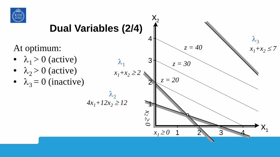
x1+x2 ≥ 2
x2 ≥ 0
4x1+12x2 ≥ 12
x1 ≥ 0
z = 20
z = 30
z = 40
λ1
λ2
x1+x2 ≤ 7 λ3
At optimum: • λ1 > 0 (active) • λ2 > 0 (active) • λ3 = 0 (inactive)
Dual Variables (3/4)
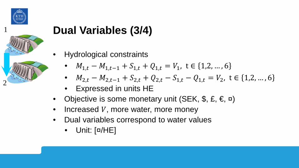
• Hydrological constraints • 𝑀1,𝑡 − 𝑀1,𝑡−1 + 𝑆1,𝑡 + 𝑄1,𝑡 = 𝑉1, t ∈ 1,2, … , 6 • 𝑀2,𝑡 − 𝑀2,𝑡−1 + 𝑆2,𝑡 + 𝑄2,𝑡 − 𝑆1,𝑡 − 𝑄1,𝑡 = 𝑉2, t ∈ 1,2, … , 6 • Expressed in units HE
• Objective is some monetary unit (SEK, $, £, €, ¤) • Increased 𝑉, more water, more money • Dual variables correspond to water values
• Unit: [¤/HE]
1
2
Dual Variables (4/4)
• Constraint for contracted load
• � 𝜇𝑖𝑖𝑄𝑖𝑖𝑡𝑖,𝑖
= 𝐷𝑡 , 𝑡 ∈ 1,2, . . . , 6
• Unit MWh • Objective still in monetary units • Increased 𝐷,
• Increased production cost, or • Less water left • Objective decreases
• Dual variables reflects marginal production costs • Unit: [¤/MWh]
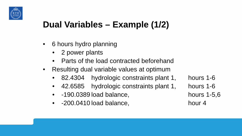
Dual Variables – Example (1/2)
• 6 hours hydro planning • 2 power plants • Parts of the load contracted beforehand
• Resulting dual variable values at optimum • 82.4304 hydrologic constraints plant 1, hours 1-6 • 42.6585 hydrologic constraints plant 1, hours 1-6 • -190.0389 load balance, hours 1-5,6 • -200.0410 load balance, hour 4
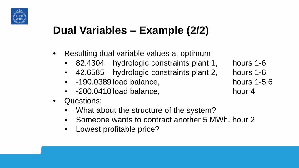
Dual Variables – Example (2/2)
• Resulting dual variable values at optimum • 82.4304 hydrologic constraints plant 1, hours 1-6 • 42.6585 hydrologic constraints plant 2, hours 1-6 • -190.0389 load balance, hours 1-5,6 • -200.0410 load balance, hour 4
• Questions: • What about the structure of the system? • Someone wants to contract another 5 MWh, hour 2 • Lowest profitable price?
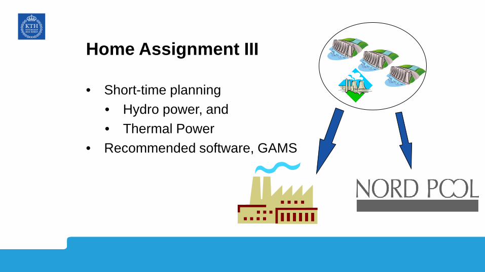
Home Assignment III
• Short-time planning • Hydro power, and • Thermal Power
• Recommended software, GAMS

GAMS (1/5)
• Algebraic modelling software • Solving optimization problems, mainly • Also CNS, and various KKT things
• Typical structure of a GAMS-model • Define sets • Define parameters • Define variables • Continues …
GAMS (2/5)
• Typical structure of a GAMS-model • Continued …
– Variable types • Free (default) • Positive (i.e. nonnegative) • Negative (i.e. nonpositive) • Continues …
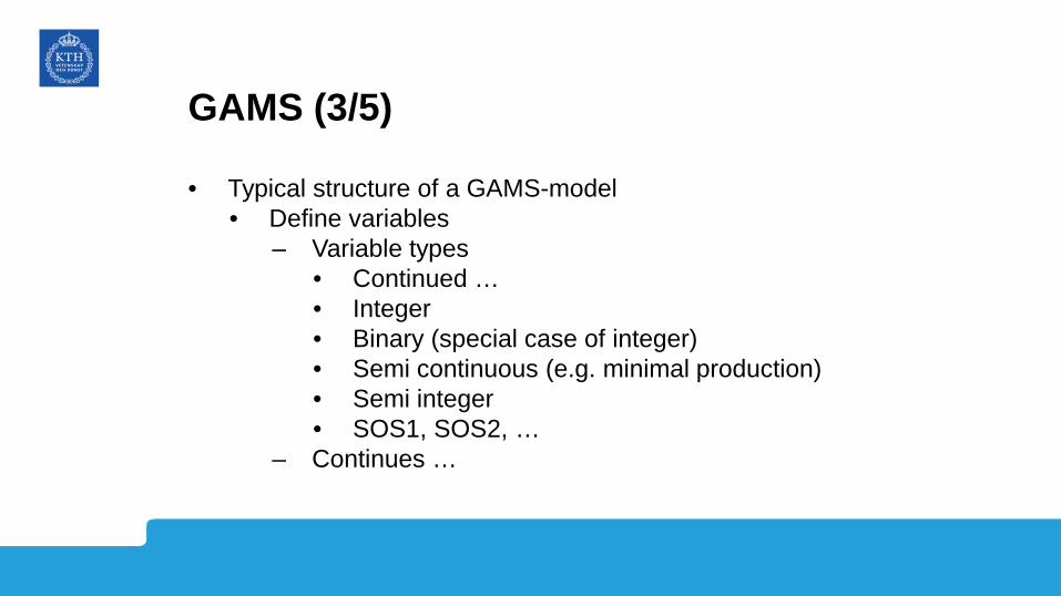
GAMS (3/5)
• Typical structure of a GAMS-model • Define variables
– Variable types • Continued … • Integer • Binary (special case of integer) • Semi continuous (e.g. minimal production) • Semi integer • SOS1, SOS2, …
– Continues …
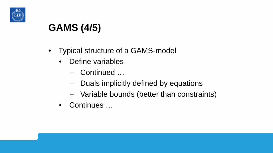
GAMS (4/5)
• Typical structure of a GAMS-model • Define variables
– Continued … – Duals implicitly defined by equations – Variable bounds (better than constraints)
• Continues …
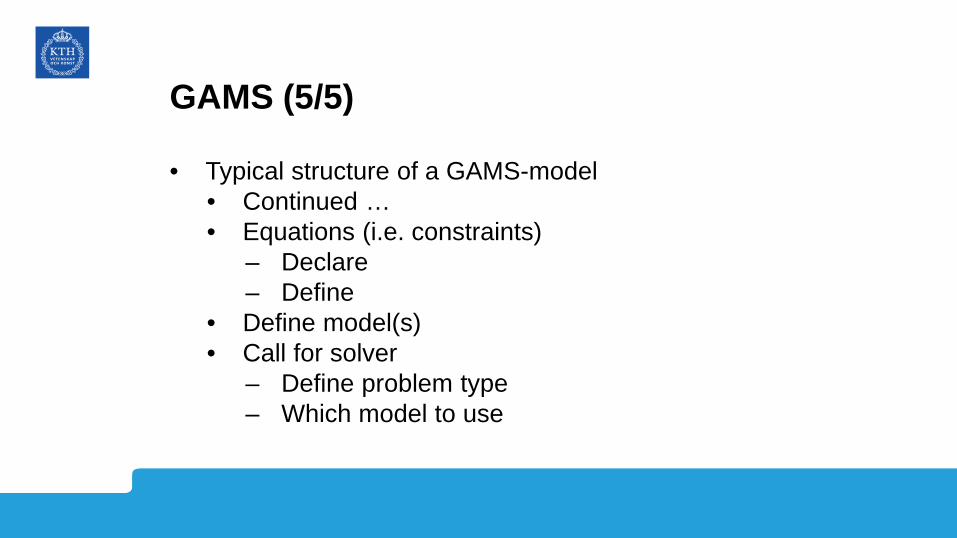
GAMS (5/5)
• Typical structure of a GAMS-model • Continued … • Equations (i.e. constraints)
– Declare – Define
• Define model(s) • Call for solver
– Define problem type – Which model to use

Example 5.6 (1/8)
• Given • Two hydro power plants • Contracted load the 6 following hours
– 90, 98, 104, 112, 100, 80 MWh – During this period, no further production!
• Reservoirs 50% filled before first hour • Water saved after planning period
– Used for most efficient production – Sold for 185 SEK/MWh
• Water transport times neglected
1
2
1
2
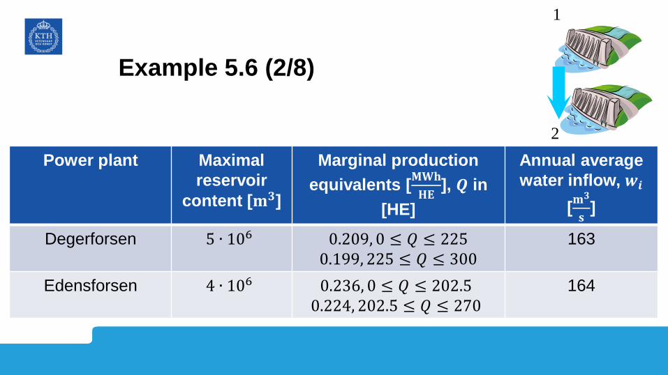
Example 5.6 (2/8)
1
2 Power plant Maximal
reservoir content [𝐦𝟑]
Marginal production equivalents [𝐌𝐌𝐌
𝐇𝐇], 𝑸 in
[HE]
Annual average water inflow, 𝒘𝒊
[𝐦𝟑
𝐬]
Degerforsen 5 ∙ 106 0.209, 0 ≤ 𝑄 ≤ 225 0.199, 225 ≤ 𝑄 ≤ 300
163
Edensforsen 4 ∙ 106 0.236, 0 ≤ 𝑄 ≤ 202.5 0.224, 202.5 ≤ 𝑄 ≤ 270
164
Example 5.6 (3/8)
• Model creation • Indices
– Power Plants, 𝑖 ∈ 1,2 – Segments, 𝑗 ∈ 1,2 – Hours, 𝑡 ∈ 1,2, … , 6
• Continued …
1
2
1
2
Example 5.6 (4/8)
• Model creation • Continues … • Parameters
– 𝜇𝑖,𝑗, 𝑄�𝑖,𝑗, 𝑀�𝑖, 𝜆𝑓, 𝑤𝑖, 𝐷𝑡, 𝑀𝑖,0
– 𝑉1 = 𝑤1 – 𝑉2 = 𝑤2 − 𝑤1
• Continued …
1
2
1
2
Example 5.6 (5/8)
• Model creation • Continues … • Variables
– Discharge, 𝑄𝑖,𝑗,𝑡, plant 𝑖, segment 𝑗, hour 𝑡.
– Spillage, 𝑆𝑖,𝑡, plant 𝑖, hour 𝑡 – Reservoir content, 𝑀𝑖,𝑡, plant 𝑖, end of hour 𝑡
• Continued …
1
2
1
2
Example 5.6 (6/8)
• Model creation • Variables • Continues …
– Variable limits – 0 ≤ 𝑄𝑖,𝑖,𝑡 ≤ 𝑄�𝑖,𝑖 – 0 ≤ 𝑆𝑖,𝑡 – 0 ≤ 𝑀𝑖,𝑡 ≤ 𝑀�𝑖
• Continued …
1
2
1
2
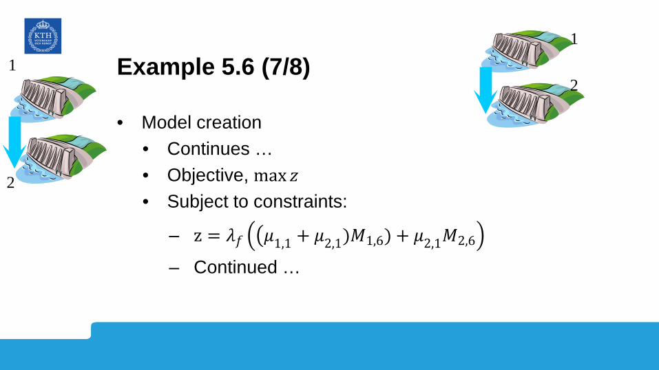
Example 5.6 (7/8)
• Model creation • Continues … • Objective, max 𝑧 • Subject to constraints:
– z = 𝜆𝑓 �𝜇1,1 + 𝜇2,1)𝑀1,6) + 𝜇2,1𝑀2,6
– Continued …
1
2
1
2
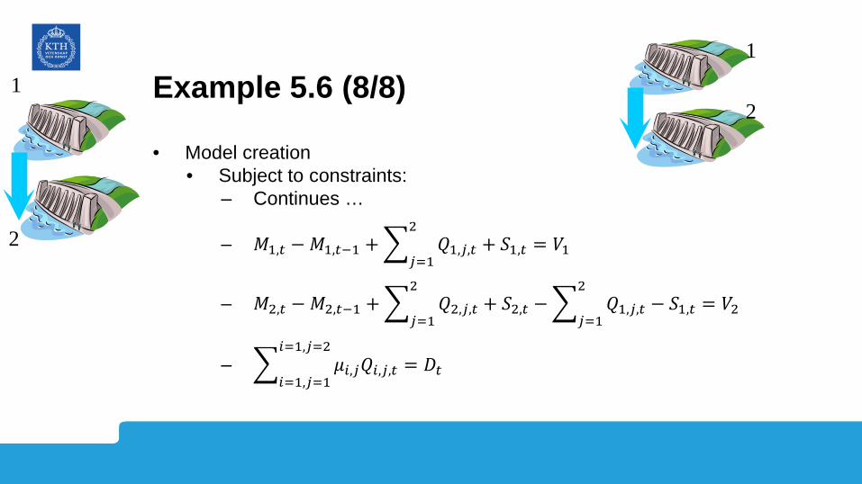
Example 5.6 (8/8)
• Model creation • Subject to constraints:
– Continues …
– 𝑀1,𝑡 − 𝑀1,𝑡−1 + � 𝑄1,𝑖,𝑡
2
𝑖=1+ 𝑆1,𝑡 = 𝑉1
– 𝑀2,𝑡 − 𝑀2,𝑡−1 + � 𝑄2,𝑖,𝑡
2
𝑖=1+ 𝑆2,𝑡 −� 𝑄1,𝑖,𝑡
2
𝑖=1− 𝑆1,𝑡 = 𝑉2
– � 𝜇𝑖,𝑖𝑄𝑖,𝑖,𝑡 = 𝐷𝑡𝑖=1,𝑖=2
𝑖=1,𝑖=1
1
2
1
2
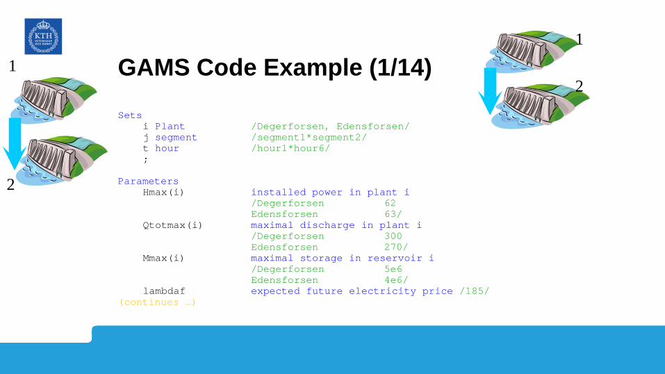
GAMS Code Example (1/14)
Sets i Plant /Degerforsen, Edensforsen/ j segment /segment1*segment2/ t hour /hour1*hour6/ ; Parameters Hmax(i) installed power in plant i /Degerforsen 62 Edensforsen 63/ Qtotmax(i) maximal discharge in plant i /Degerforsen 300 Edensforsen 270/ Mmax(i) maximal storage in reservoir i /Degerforsen 5e6 Edensforsen 4e6/ lambdaf expected future electricity price /185/ (continues …)
1
2
1
2
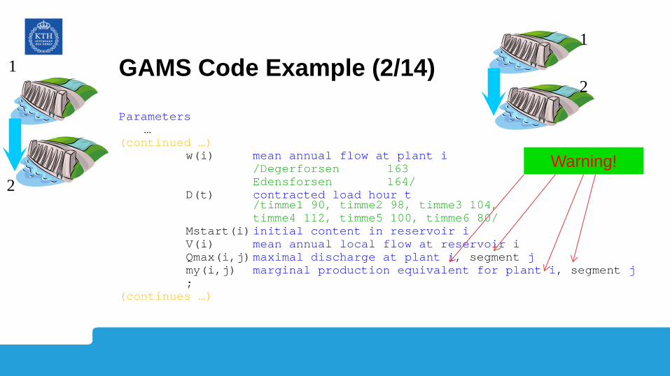
GAMS Code Example (2/14)
Parameters … (continued …) w(i) mean annual flow at plant i /Degerforsen 163 Edensforsen 164/ D(t) contracted load hour t /timme1 90, timme2 98, timme3 104, timme4 112, timme5 100, timme6 80/ Mstart(i) initial content in reservoir i V(i) mean annual local flow at reservoir i Qmax(i,j) maximal discharge at plant i, segment j my(i,j) marginal production equivalent for plant i, segment j ; (continues …)
1
2
1
2
Warning!
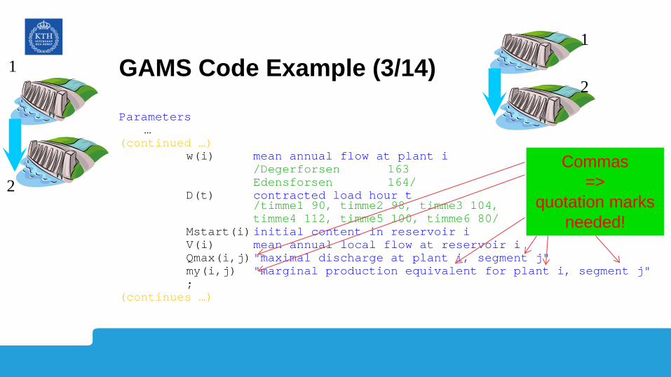
GAMS Code Example (3/14)
Parameters … (continued …) w(i) mean annual flow at plant i /Degerforsen 163 Edensforsen 164/ D(t) contracted load hour t /timme1 90, timme2 98, timme3 104, timme4 112, timme5 100, timme6 80/ Mstart(i) initial content in reservoir i V(i) mean annual local flow at reservoir i Qmax(i,j) "maximal discharge at plant i, segment j" my(i,j) "marginal production equivalent for plant i, segment j" ; (continues …)
1
2
1
2
Commas =>
quotation marks needed!
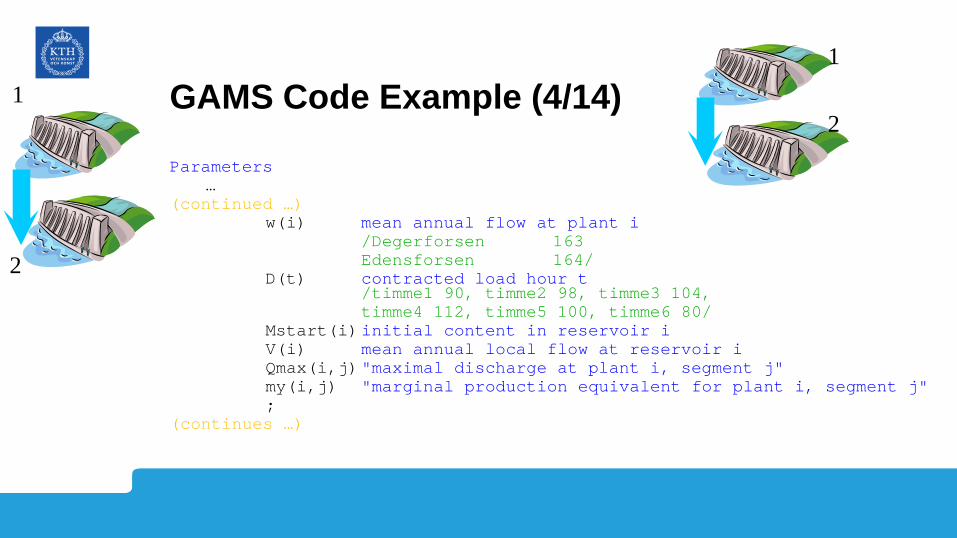
GAMS Code Example (4/14)
Parameters … (continued …) w(i) mean annual flow at plant i /Degerforsen 163 Edensforsen 164/ D(t) contracted load hour t /timme1 90, timme2 98, timme3 104, timme4 112, timme5 100, timme6 80/ Mstart(i) initial content in reservoir i V(i) mean annual local flow at reservoir i Qmax(i,j) "maximal discharge at plant i, segment j" my(i,j) "marginal production equivalent for plant i, segment j" ; (continues …)
1
2
1
2
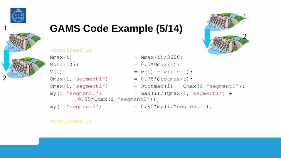
GAMS Code Example (5/14)
(continued …) Mmax(i) = Mmax(i)/3600; Mstart(i) = 0.5*Mmax(i); V(i) = w(i) - w(i - 1); Qmax(i,"segment1") = 0.75*Qtotmax(i); Qmax(i,"segment2") = Qtotmax(i) - Qmax(i,"segment1"); my(i,"segment1") = max(i)/(Qmax(i,"segment1") + 0.95*Qmax(i,"segment2")); my(i,"segment2") = 0.95*my(i,"segment1"); (continues …)
1
2
1
2
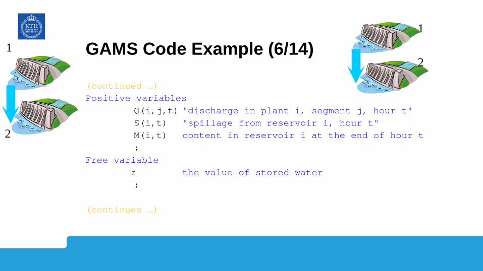
GAMS Code Example (6/14)
(continued …) Positive variables Q(i,j,t) "discharge in plant i, segment j, hour t" S(i,t) "spillage from reservoir i, hour t" M(i,t) content in reservoir i at the end of hour t ; Free variable z the value of stored water ; (continues …)
1
2
1
2
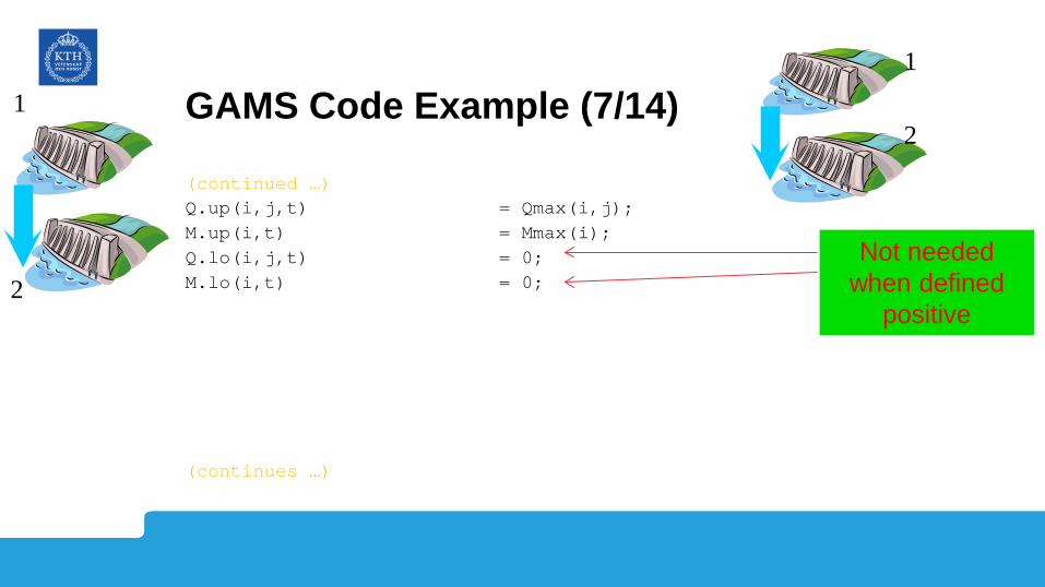
GAMS Code Example (7/14)
(continued …) Q.up(i,j,t) = Qmax(i,j); M.up(i,t) = Mmax(i); Q.lo(i,j,t) = 0; M.lo(i,t) = 0; (continues …)
1
2
1
2
Not needed when defined
positive
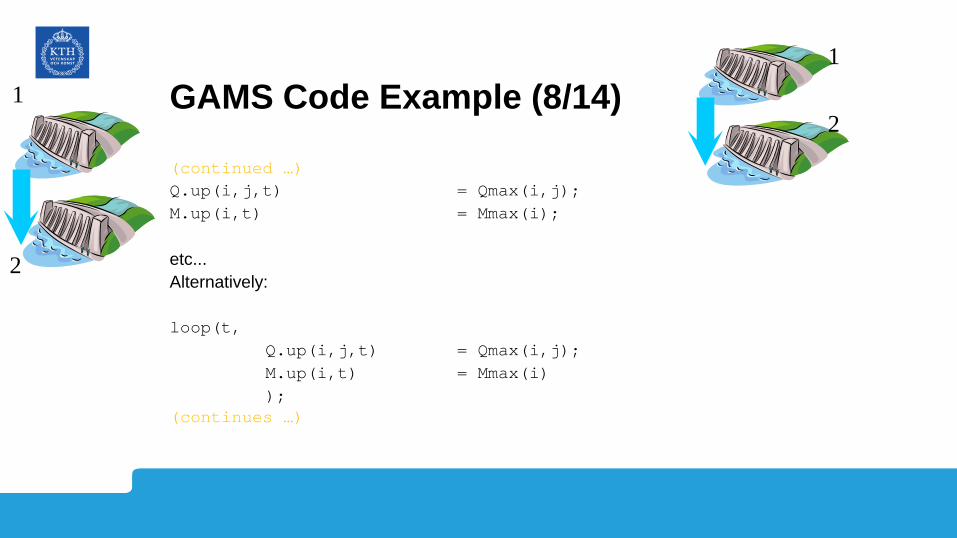
GAMS Code Example (8/14)
(continued …) Q.up(i,j,t) = Qmax(i,j); M.up(i,t) = Mmax(i); etc... Alternatively: loop(t, Q.up(i,j,t) = Qmax(i,j); M.up(i,t) = Mmax(i) ); (continues …)
1
2
1
2
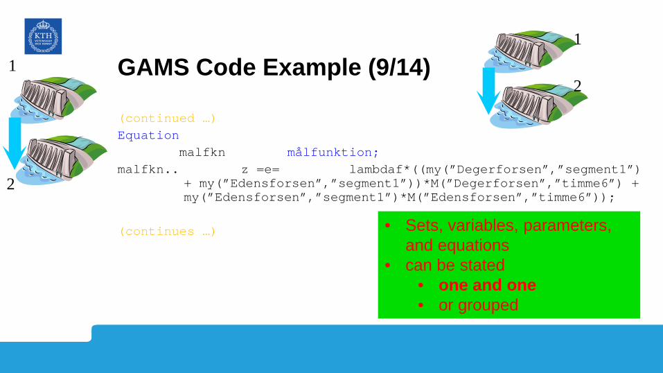
GAMS Code Example (9/14)
(continued …) Equation malfkn målfunktion; malfkn.. z =e= lambdaf*((my(”Degerforsen”,”segment1”) + my(”Edensforsen”,”segment1”))*M(”Degerforsen”,”timme6”) + my(”Edensforsen”,”segment1”)*M(”Edensforsen”,”timme6”)); (continues …)
1
2
1
2
• Sets, variables, parameters, and equations
• can be stated • one and one • or grouped

GAMS Code Example (10/14)
(continued …) Equations hydbal(i,t) "hydrological balance for plant i, hour t" loadbal(t) load balance for hour t ; hydbal(i,t) .. M(i,t) =e= M(i,t - 1) + Mstart(i)$(ord(t) = 1) – sum(j,Q(i,j,t)) – S(i,t) + sum(j,Q(i - 1,j,t)) + S(i - 1,t) - V(i); loadbal(t) .. sum((i,j),my(i,j)*Q(i,j,t)) =e= D(t) ; (continues …)
1
2
1
2
• Sets, variables, parameters, and equations
• can be stated • one and one • or grouped
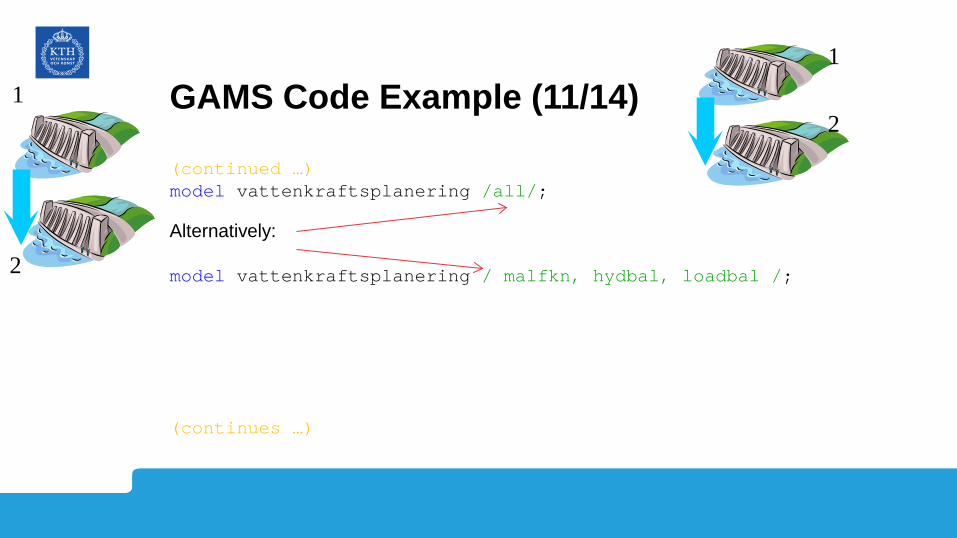
GAMS Code Example (11/14)
(continued …) model vattenkraftsplanering /all/; Alternatively: model vattenkraftsplanering / malfkn, hydbal, loadbal /; (continues …)
1
2
1
2
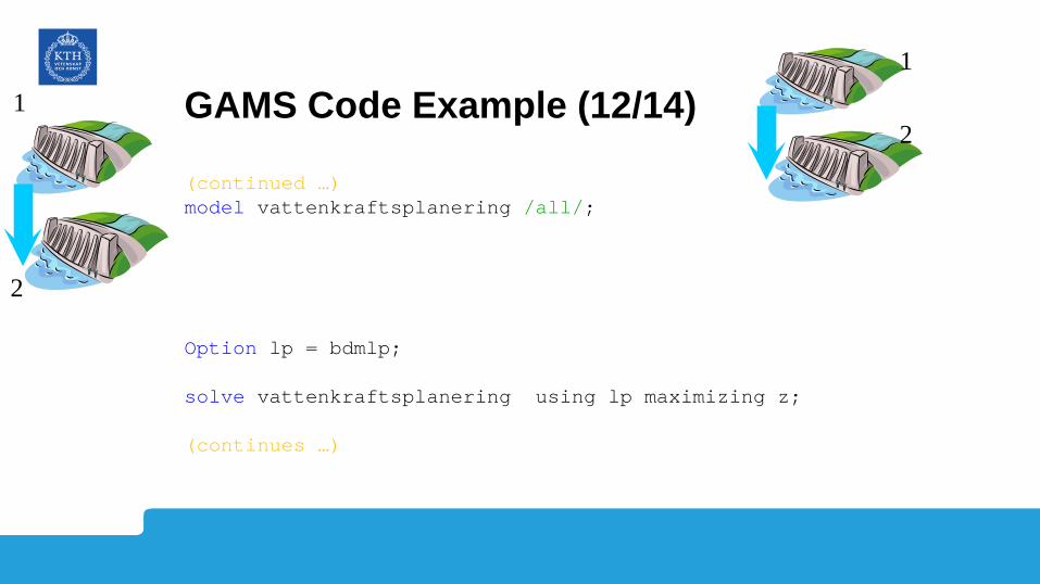
GAMS Code Example (12/14)
(continued …) model vattenkraftsplanering /all/; Option lp = bdmlp; solve vattenkraftsplanering using lp maximizing z; (continues …)
1
2
1
2
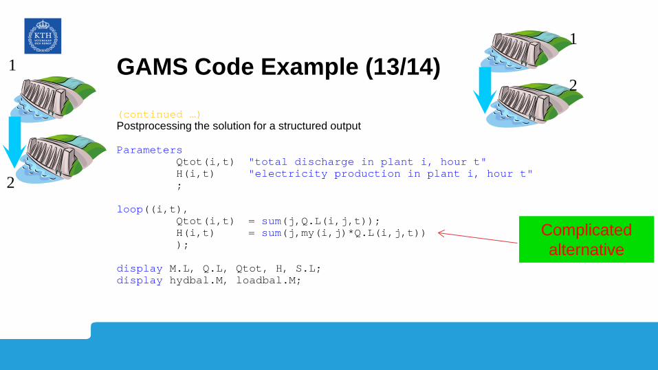
GAMS Code Example (13/14)
(continued …) Postprocessing the solution for a structured output Parameters Qtot(i,t) "total discharge in plant i, hour t" H(i,t) "electricity production in plant i, hour t" ; loop((i,t), Qtot(i,t) = sum(j,Q.L(i,j,t)); H(i,t) = sum(j,my(i,j)*Q.L(i,j,t)) ); display M.L, Q.L, Qtot, H, S.L; display hydbal.M, loadbal.M;
1
2
1
2
Complicated alternative
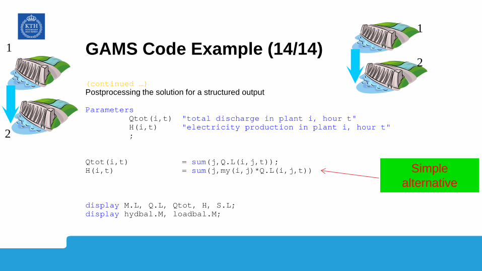
GAMS Code Example (14/14)
(continued …) Postprocessing the solution for a structured output Parameters Qtot(i,t) "total discharge in plant i, hour t" H(i,t) "electricity production in plant i, hour t" ; Qtot(i,t) = sum(j,Q.L(i,j,t)); H(i,t) = sum(j,my(i,j)*Q.L(i,j,t)) display M.L, Q.L, Qtot, H, S.L; display hydbal.M, loadbal.M;
1
2
1
2
Simple alternative

Go Home
• The show is over!


![Modelling Minimum Pressure Height in Short-term … · SHOP (Short-term Hydro Operation Planning) [1] ... Research’s state-of-the-art models for hydropower and hydro thermal scheduling](https://img.pdfslide.net/doc/110x75/5addf3457f8b9ae1408daa13/modelling-minimum-pressure-height-in-short-term-short-term-hydro-operation.jpg)