Embed Size (px)
Citation preview

Lecture 9: Linear Quadratic Control
Dynamic Programming
Riccati equation
Optimal State Feedback
Stability and Robustness
The sections 9.1-9.4 + 5.7 in the book treat essentially the same
material as we cover in lecture 9-11. However, the main derivation of
the LQG controller in appendix 9A is different.
Automatic Control LTH FRTN10 Multivariable Control, Lecture 9
Course outline
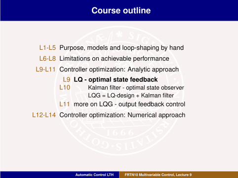
L1-L5 Purpose, models and loop-shaping by hand
L6-L8 Limitations on achievable performance
L9-L11 Controller optimization: Analytic approach
L9 LQ - optimal state feedback
L10 Kalman filter - optimal state observer
LQG = LQ-design + Kalman filter
L11 more on LQG - output feedback control
L12-L14 Controller optimization: Numerical approach
Automatic Control LTH FRTN10 Multivariable Control, Lecture 9
Math Repetition
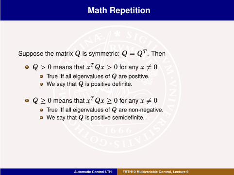
Suppose the matrix Q is symmetric: Q = QT . Then
Q > 0 means that xTQx > 0 for any x ,= 0True iff all eigenvalues of Q are positive.
We say that Q is positive definite.
Q ≥ 0 means that xTQx ≥ 0 for any x ,= 0True iff all eigenvalues of Q are non-negative.
We say that Q is positive semidefinite.
Automatic Control LTH FRTN10 Multivariable Control, Lecture 9
Math Repetition
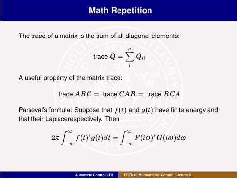
The trace of a matrix is the sum of all diagonal elements:
trace Q =n∑
i
Qii
A useful property of the matrix trace:
trace ABC = trace CAB = trace BCA
Parseval’s formula: Suppose that f (t) and �(t) have finite energy and
that their Laplacerespectively. Then
2π
∫ ∞
−∞f (t)∗�(t)dt =
∫ ∞
−∞F(iω )∗G(iω )dω
Automatic Control LTH FRTN10 Multivariable Control, Lecture 9
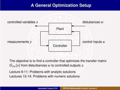
A General Optimization Setup
Plant
Controller
✛ ✛
✛
✲
control inputs u
controlled variables z
measurements y
distubances w
The objective is to find a controller that optimizes the transfer matrix
Gzw(s) from disturbances w to controlled outputs z.
Lecture 9-11: Problems with analytic solutions
Lectures 12-14: Problems with numeric solutions
Automatic Control LTH FRTN10 Multivariable Control, Lecture 9
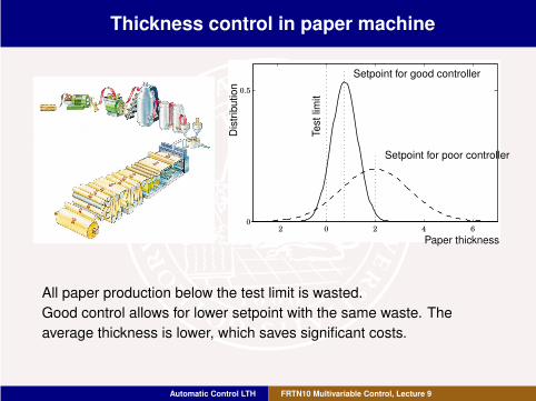
Thickness control in paper machine
-2 0 2 4 6
0
0.5
Dis
trib
ution
Setpoint for good controller
Setpoint for poor controller
Testlim
it
Paper thickness
All paper production below the test limit is wasted.
Good control allows for lower setpoint with the same waste. The
average thickness is lower, which saves significant costs.
Automatic Control LTH FRTN10 Multivariable Control, Lecture 9
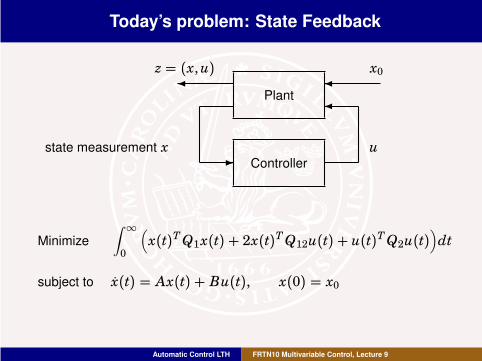
Today’s problem: State Feedback
Plant
Controller
✛ ✛
✛
✲
u
z = (x,u) x0
state measurement x
Minimize
∫ ∞
0
(
x(t)TQ1x(t) + 2x(t)TQ12u(t) + u(t)TQ2u(t))
dt
subject to x(t) = Ax(t) + Bu(t), x(0) = x0
Automatic Control LTH FRTN10 Multivariable Control, Lecture 9
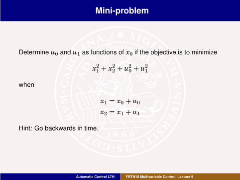
Mini-problem
Determine u0 and u1 as functions of x0 if the objective is to minimize
x21 + x22 + u20 + u21
when
x1 = x0 + u0x2 = x1 + u1
Hint: Go backwards in time.
Automatic Control LTH FRTN10 Multivariable Control, Lecture 9
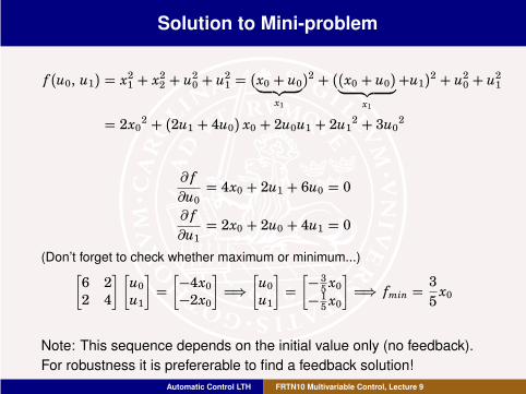
Solution to Mini-problem
f (u0, u1) = x21 + x22 + u20 + u21 = (x0 + u0︸ ︷︷ ︸
x1
)2 + ((x0 + u0)︸ ︷︷ ︸
x1
+u1)2 + u20 + u21
= 2x02 + (2u1 + 4u0) x0 + 2u0u1 + 2u12 + 3u02
� f�u0
= 4x0 + 2u1 + 6u0 = 0
� f�u1
= 2x0 + 2u0 + 4u1 = 0
(Don’t forget to check whether maximum or minimum...)[6 2
2 4
] [u0u1
]
=[−4x0−2x0
]
=[[u0u1
]
=[− 35x0
− 15x0
]
=[ fmin =3
5x0
Note: This sequence depends on the initial value only (no feedback).
For robustness it is prefererable to find a feedback solution!
Automatic Control LTH FRTN10 Multivariable Control, Lecture 9

Quadratic Optimal Cost
The optimal cost on the time interval [T1,∞] is quadratic:
xTSx = minu
∫ ∞
T1
x
u
T
Q1 Q12QT12 Q2
x
u
dt
when
{
x = Ax+ Bux(T1) = x
Automatic Control LTH FRTN10 Multivariable Control, Lecture 9

Dynamic programming, Richard E. Bellman 1957
T1 T1 + ǫ T
An optimal trajectory on the time in-
terval [T1,T ] must be optimal also on
each of the subintervals [T1,T1 + ǫ]and [T1 + ǫ,T ].
Automatic Control LTH FRTN10 Multivariable Control, Lecture 9

Dynamic programming in linear quadratic control
x(T1) = x, x(T1 + ǫ) = x + (Ax + Bu)ǫ
xTSx = minu
∫ ∞
T1
x
u
T
Q1 Q12QT12 Q2
x
u
dt
= minu
{
x
u
T
Q1 Q12QT12 Q2
x
u
ǫ+∫ ∞
T1+ǫ
x
u
T
Q1 Q12QT12 Q2
x
u
dt
}
= minu
{
x
u
T
Q1 Q12QT12 Q2
x
u
ǫ+[
x + (Ax + Bu)ǫ]T
S
[
x + (Ax + Bu)ǫ]}
by definition of S. Neglecting ǫ2 gives Bellman’s equation:
0 = minu
[(
xTQ1x + 2xTQ12u+ uTQ2u)
+ 2xTS(Ax + Bu
)]
Automatic Control LTH FRTN10 Multivariable Control, Lecture 9
Lecture 9: Linear Quadratic Control
Dynamic Programming
Riccati equation
Optimal State Feedback
Stability and Robustness
Automatic Control LTH FRTN10 Multivariable Control, Lecture 9

Completion of squares
The scalar case: Suppose c > 0.
ax2 + 2bxu+ cu2 = x(
a− b2
c
)
x +(
u+ bcx
)
c
(
u+ bcx
)
is minimized by u = − bcx. The minimum is
(
a− b2/c)
x2.
The matrix case: Suppose Qu > 0. Then
xTQxx + 2xTQxuu+ uTQuu= (u+ Q−1u QTxux)TQu(u+ Q−1u QTxux) + xT(Qx − QxuQ−1u QTxu)x
is minimized by u = −Q−1u QTxux. The minimum is
xT(Qx − QxuQ−1u QTxu)x.
Automatic Control LTH FRTN10 Multivariable Control, Lecture 9
The Riccati Equation
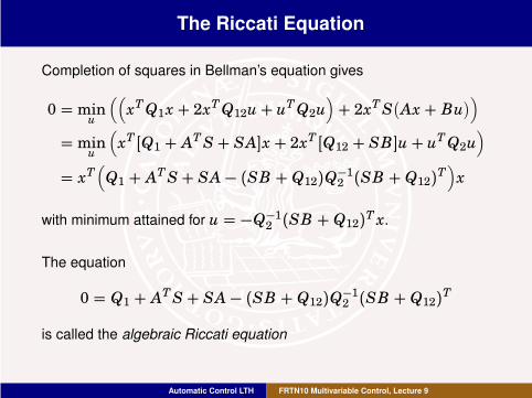
Completion of squares in Bellman’s equation gives
0 = minu
((
xTQ1x + 2xTQ12u+ uTQ2u)
+ 2xTS(Ax + Bu
))
= minu
(
xT [Q1 + ATS+ SA]x + 2xT [Q12 + SB]u+ uTQ2u)
= xT(
Q1 + ATS+ SA− (SB + Q12)Q−12 (SB + Q12)T)
x
with minimum attained for u = −Q−12 (SB + Q12)T x.
The equation
0 = Q1 + ATS+ SA− (SB + Q12)Q−12 (SB + Q12)T
is called the algebraic Riccati equation
Automatic Control LTH FRTN10 Multivariable Control, Lecture 9

Jocopo Francesco Riccati, 1676–1754
Automatic Control LTH FRTN10 Multivariable Control, Lecture 9
Lecture 9: Linear Quadratic Control
Dynamic Programming
Riccati equation
Optimal State Feedback
Stability and Robustness
Automatic Control LTH FRTN10 Multivariable Control, Lecture 9
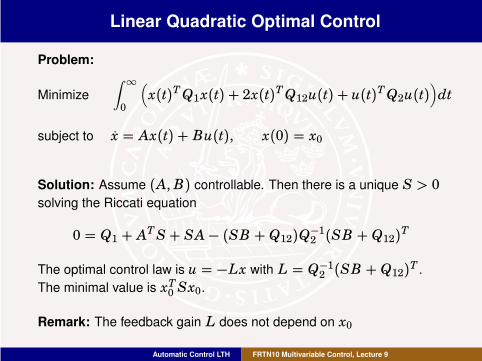
Linear Quadratic Optimal Control
Problem:
Minimize
∫ ∞
0
(
x(t)TQ1x(t) + 2x(t)TQ12u(t) + u(t)TQ2u(t))
dt
subject to x = Ax(t) + Bu(t), x(0) = x0
Solution: Assume (A, B) controllable. Then there is a unique S > 0solving the Riccati equation
0 = Q1 + ATS+ SA− (SB + Q12)Q−12 (SB + Q12)T
The optimal control law is u = −Lx with L = Q−12 (SB + Q12)T .
The minimal value is xT0 Sx0.
Remark: The feedback gain L does not depend on x0
Automatic Control LTH FRTN10 Multivariable Control, Lecture 9
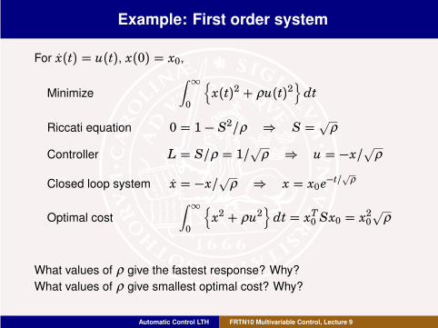
Example: First order system
For x(t) = u(t), x(0) = x0,
Minimize
∫ ∞
0
{
x(t)2 + ρu(t)2}
dt
Riccati equation 0 = 1− S2/ρ [ S = √ρ
Controller L = S/ρ = 1/√ρ [ u = −x/√ρ
Closed loop system x = −x/√ρ [ x = x0e−t/√
ρ
Optimal cost
∫ ∞
0
{
x2 + ρu2}
dt = xT0 Sx0 = x20√
ρ
What values of ρ give the fastest response? Why?
What values of ρ give smallest optimal cost? Why?
Automatic Control LTH FRTN10 Multivariable Control, Lecture 9
Lecture 9: Linear Quadratic Control
Dynamic Programming
Riccati equation
Optimal State Feedback
Stability and Robustness
Automatic Control LTH FRTN10 Multivariable Control, Lecture 9
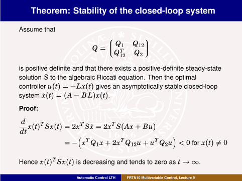
Theorem: Stability of the closed-loop system
Assume that
Q =
Q1 Q12QT12 Q2
is positive definite and that there exists a positive-definite steady-state
solution S to the algebraic Riccati equation. Then the optimal
controller u(t) = −Lx(t) gives an asymptotically stable closed-loop
system x(t) = (A− BL)x(t).Proof:
d
dtx(t)TSx(t) = 2xTSx = 2xTS(Ax + Bu)
= −(
xTQ1x + 2xTQ12u+ uTQ2u)
< 0 for x(t) ,= 0
Hence x(t)TSx(t) is decreasing and tends to zero as t→∞.
Automatic Control LTH FRTN10 Multivariable Control, Lecture 9
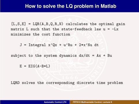
How to solve the LQ problem in Matlab
[L,S,E] = LQR(A,B,Q,R,N) calculates the optimal gain
matrix L such that the state-feedback law u = -Lx
minimizes the cost function
J = Integral x’Qx + u’Ru + 2*x’Nu dt
subject to the system dynamics dx/dt = Ax + Bu
E = EIG(A-B*L)
LQRD solves the corresponding discrete time problem
Automatic Control LTH FRTN10 Multivariable Control, Lecture 9
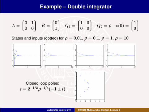
Example – Double integrator
A =
0 1
0 0
B =
0
1
Q1 =
1 0
0 0
Q2 = ρ x(0) =
1
0
States and inputs (dotted) for ρ = 0.01, ρ = 0.1, ρ = 1, ρ = 10
0 5 10-4
-2
0
2
4
0 5 10-4
-2
0
2
4
0 5 10-4
-2
0
2
4
0 5 10-4
-2
0
2
4
Closed loop poles:
s = 2−1/2ρ−1/4(−1± i)
-3 -2 -1 0 1 2 3-3
-2
-1
0
1
2
3
Automatic Control LTH FRTN10 Multivariable Control, Lecture 9
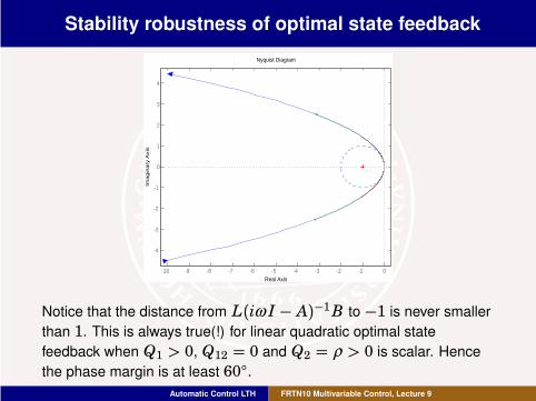
Stability robustness of optimal state feedback
-10 -9 -8 -7 -6 -5 -4 -3 -2 -1 0
-4
-3
-2
-1
0
1
2
3
4
Nyquist Diagram
Real Axis
Imagin
ary
Axi
s
Notice that the distance from L(iω I − A)−1B to −1 is never smaller
than 1. This is always true(!) for linear quadratic optimal state
feedback when Q1 > 0, Q12 = 0 and Q2 = ρ > 0 is scalar. Hence
the phase margin is at least 60○.Automatic Control LTH FRTN10 Multivariable Control, Lecture 9
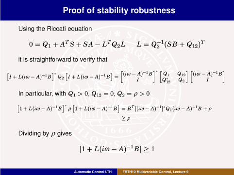
Proof of stability robustness
Using the Riccati equation
0 = Q1 + ATS+ SA− LTQ2L L = Q−12 (SB + Q12)T
it is straightforward to verify that
[I + L(iω − A)−1B
]∗Q2[I + L(iω − A)−1B
]=[(iω − A)−1B
I
]∗ [Q1 Q12Q∗12
Q2
][(iω − A)−1BI
]
In particular, with Q1 > 0, Q12 = 0, Q2 = ρ > 0[1+ L(iω − A)−1B
]∗
ρ[1+ L(iω − A)−1B
]= BT [(iω − A)−1]∗Q1(iω − A)−1B + ρ
≥ ρ
Dividing by ρ gives
p1+ L(iω − A)−1Bp ≥ 1
Automatic Control LTH FRTN10 Multivariable Control, Lecture 9
Lecture 9: Summary
Dynamic Programming
Riccati equation
Optimal State Feedback
Stability and Robustness
Automatic Control LTH FRTN10 Multivariable Control, Lecture 9

Next Lecture: Linear Quadratic Gaussian Control
Plant
Controller
✛ ✛
✛
✲
control inputs u
controlled variables z
measurements y
distubances w
For a linear plant, minimize a quadratic function of the map from
disturbance w to controlled variable z
Automatic Control LTH FRTN10 Multivariable Control, Lecture 9