Lecture: Demand

Demand

Uncompensated Demand

By de�nition demand tells us how much a consumer is willing to buyat a given price, holding constant other factors (such as tastes andpreferences, income, and prices of complements and substitutes).

Take the utility maximization problem analyzed earlier.

We solved for the optimal quantities as functions of prices and income.That is, we have found the consumer�s uncompensated demandfunctions for these goods:

q1 = Z(p1, p2, Y)q2 = B(p1, p2, Y).

In the Cobb-Douglas example, the uncompensated demands were

q1 = αY/p1, q2 = (1� α)Y/p2.

The two goods are neither complements nor substitutes: the demanddepends only on the good�s own price.

Demand

Uncompensated Demand (Continued)

Suppose that we double all prices and income. What will happen touncompensated demand?

The utility maximization problem becomes

maxq1,q2

U(q1, q2)

s.t. 2p1q1 + 2p2q2 = 2Y.

Note that the new budget constraint is equivalent to the original one.So the two problems will have identical solutions.

If we multiply all prices and income by some number, uncompensateddemand will not change!

Consider our Cobb-Douglas example:

q1 =α2Y2p1

=αYp1, q2 =

(1� α)2Y2p2

=(1� α)Y

p2.

Demand

Constructing the Uncompensated Demand Curve

Now we use a graphical approach to construct the uncompensateddemand curve.

If we increase a good�s price while holding other prices, tastes andincome constant, the budget constraint will rotate.

Thus, the optimal consumption bundle will change as the budgetconstraint rotates.

If we connect all optimal bundles in this graph, we will get the priceconsumption curve.From the price consumption curve we can obtain the demand curve.

Demand

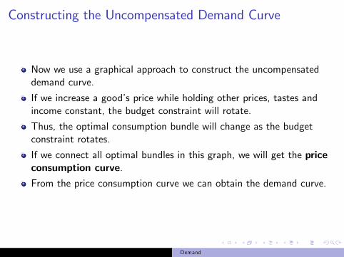
Constructing the Uncompensated Demand Curve (Cont.)On the graph below, we vary the price of good 1 (beer)

Connecting the equilibrium bundles e1, e2, e3 yields the priceconsumption curve.

Demand

Constructing the Uncompensated Demand Curve (Cont.)

We can translate the price consumption curve from a (q1, q2)-diagramto a (q1, p1)-diagram. This gives us the demand for beer!

Demand

Constructing the Uncompensated Demand Curve (Cont.)

For some preferences the demand curve can be upward sloping!

Such goods are called Gi¤en goods.

xDemand curve

U1

U2

U3

1x2x3x

P2

P1

P3

Pric

e of

x

Price consumptioncurveG

ood

y

Good x1xP

I

2xPI

3xPI

Px falls

Demand

How Income Changes Shift Uncompensated Demand

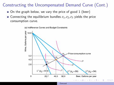
In an earlier lecture, we argued that a change in income causes a shiftof the (uncompensated) demand curve.

Now we examine how consumer behavior changes when incomechanges, while keeping prices and tastes constant.

A rise in income leads to a parallel outward shift of the budget line.

Thus, as income changes, the optimal bundle will change.

If we connect the optimal bundles for all income levels, we get theincome-consumption curve.

Demand

How Income Changes Shift Demand (Continued)

On the graph below, we vary the consumer�s income.

Connecting the equilibrium bundles e1, e2, e3 gives us theincome-consumption curve.

Demand

How Income Changes Shift Demand (Continued)We can plot the optimal quantity of beer in (q1, p1)-space.The change in income shifts the demand curve.

Demand

How Income Changes Shift Demand (Continued)We can plot the income-consumption curve in a (q1, Y)-diagram.This will give us the Engel curve.

Demand

How Income Changes Shift Demand (Continued)

It is possible that the income-consumption curve is downward-sloping,and hence the Engel curve could be downward-sloping.

x

Wee

kly 

inco

me

I

A”B”

C”

I1

I2

I3

I4

Engel Curve

D”

x

Incomeconsumption

curve

U1

U2

U3

U4

y

BL1

BL2BL3

BL4A

B

C

D

Demand

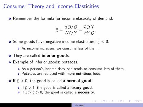
Consumer Theory and Income Elasticities

Remember the formula for income elasticity of demand:

ξ =∆Q/Q∆Y/Y

=∂Q∂Y

YQ.

Some goods have negative income elasticities: ξ < 0.

As income increases, we consume less of them.

They are called inferior goods.Example of inferior goods: potatoes.

As a person�s income rises, she tends to consume less of them.Potatoes are replaced with more nutritious food.

If ξ > 0, the good is called a normal good.

If ξ > 1, the good is called a luxury good.If 1 > ξ > 0, the good is called a necessity.

Demand

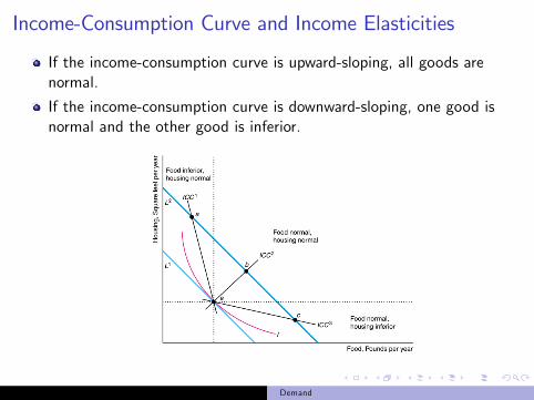
Income-Consumption Curve and Income Elasticities

If the income-consumption curve is upward-sloping, all goods arenormal.

If the income-consumption curve is downward-sloping, one good isnormal and the other good is inferior.

Demand

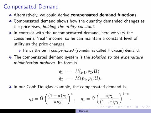
Compensated DemandAlternatively, we could derive compensated demand functions.Compensated demand shows how the quantity demanded changes asthe price rises, holding the utility constant.In contrast with the uncompensated demand, here we vary theconsumer�s "real" income, so he can maintain a constant level ofutility as the price changes.

Hence the term compensated (sometimes called Hicksian) demand.

The compensated demand system is the solution to the expenditureminimization problem. Its form is

q1 = H(p1, p2, U)q2 = M(p1, p2, U).

In our Cobb-Douglas example, the compensated demand is

q2 = U�(1� α)p1

αp2

�α

, q1 = U�

αp2

(1� α)p1

�1�α

.

Demand

Deriving Compensated Demand GraphicallySuppose that we vary px.To maintain the same level of utility, we must also vary Y accordingly!Plot the curve in a (x, px)-diagram to get compensated demand.

x

B

A

x1

CompensatedDemand

x2

px

px

px’

Demand

E¤ects of a Price Increase

Consider an increase in the price of good 1.

This has two e¤ects on the uncompensated demand of good 1.

substitution e¤ect: the change in the quantity of a good that aconsumer demands when the good�s price rises, holding other pricesand the consumer�s utility constant.

income e¤ect: the change in the quantity of a good that a consumerdemands due to the change in his "real" income, holding prices �xed.

The total e¤ect on uncompensated demand is the sum of the incomeand the substitution e¤ects.

The substitution e¤ect always goes in one direction: buy more of thegood that becomes cheaper.

The income e¤ect can go either way, depending on whether the goodis normal or inferior.

Demand

Decomposing the E¤ects Graphically

Suppose that the price of good 1 has increased.

Thus, the budget constraint rotates inward around the vertical axis.

We decompose the total e¤ect as follows.

1 Find the optimal bundle before the price change.2 Find the optimal bundle after the price change.3 Now draw an "imaginary" budget line which is parallel to the newbudget line, but tangent to the old indi¤erence curve.

The change between the two parallel lines is the income e¤ect.

The change due to rotating the budget line around the oldindi¤erence curve is the substitution e¤ect.

Demand

Decomposing the E¤ects Graphically (Continued)The e¤ects are illustrated on the graph below:

Demand

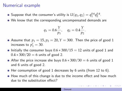
Numerical example

Suppose that the consumer�s utility is U(q1, q2) = q0.61 q0.4

2 .

We know that the corresponding uncompensated demands are

q1 = 0.6Yp1, q2 = 0.4

Yp2.

Assume that p1 = 15, p2 = 20, Y = 300. Then the price of good 1increases to p01 = 30.Initially the consumer buys 0.6 � 300/15 = 12 units of good 1 and0.4 � 300/20 = 6 units of good 2.After the price increase she buys 0.6 � 300/30 = 6 units of good 1and 6 units of good 2.

Her consumption of good 1 decreases by 6 units (from 12 to 6).

How much of this change is due to the income e¤ect and how muchdue to the substitution e¤ect?

Demand

Numerical example

Before the price increase, the consumer�s utility was U = 120.6 � 60.4.

After the price increase, how much income Y� does the consumerneed to have to attain the old level of utility U?This income would solve the equation�

0.6Y30

��0.6 �0.4Y�

20

�0.4

= 120.6 � 60.4

Solving for Y� yields Y� = 450.If the consumer had income Y� = 450, at the new price p01 he wouldbuy 0.6 � 450/30 = 9 units of good 1.The decrease from 12 to 9 is due to the substitution e¤ect.

We have maintained the "real" income constant, so the consumer�slevel of utility is unchanged.

The remaining change is due to the income e¤ect.

Demand

Price Changes and Normal Goods

Suppose the price of a normal good increases (as in slide 19).

This good would become relatively more expensive.

Thus, the substitution e¤ect says that we should consume less of it.

Furthermore, the consumer�s real income decreases (the oldconsumption bundle becomes una¤ordable).

Since the good is normal, the income e¤ects says that we shouldconsume less of it.

Thus, both e¤ects work in one direction: consume less.

The demand curve of a normal good is necessarily downward-sloping!

Demand

Price Changes and Inferior Goods

Next suppose that the price of an inferior good increases.

Then this good would become relatively more expensive.

Thus, the substitution e¤ect says that we should consume less of it.

Furthermore, the consumer�s real income decreases (the oldconsumption bundle becomes una¤ordable).

Since the good is inferior, the income e¤ects says that we shouldconsume more of it.

The two e¤ects work in di¤erent direction!

The overall e¤ect depends on which e¤ect is stronger.

Demand

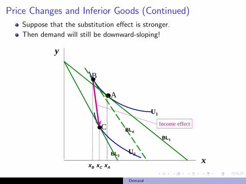
Price Changes and Inferior Goods (Continued)Suppose that the substitution e¤ect is stronger.Then demand will still be downward-sloping!

x

B

BLd

A

C

xAxC

BL1

BL2

U1

U2

xB

y

Income effect

Demand

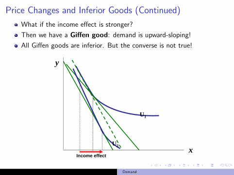
Price Changes and Inferior Goods (Continued)

What if the income e¤ect is stronger?

Then we have a Gi¤en good: demand is upward-sloping!All Gi¤en goods are inferior. But the converse is not true!

y

x

U1

U2

Income effect

Demand

Changes in Compensated versus Uncompensated Demands

Note that the substitution e¤ect is actually the change incompensated demand we get if we �x the utility at the old level!

If we set the consumer�s income to be equal to the minimizedexpenditure, the compensated demand will be the same as theuncompensated demand.

Next consider a decrease in the price of good 1.

If the good is normal, the income e¤ect will increase consumption.

Therefore, the compensated demand will increase by less than theuncompensated (will be steeper).

If the good is inferior, the income e¤ect will decrease consumption.

The compensated demand will increase by more than theuncompensated (will be �atter).

Demand

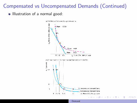
Compensated vs Uncompensated Demands (Continued)Illustration of a normal good:

Demand

The Slutsky EquationThe relationship between the total change in demand, the income andthe substitution e¤ects can be demonstrated mathematically.This relationship is known as the Slutsky equation:

∂D∂p1

=∂H∂p1

� ∂D∂Y

q1.

∂D∂p1

is the change in the uncompensated demand (the total change).∂H∂p1

is the change in the compensated demand (the substitution e¤ect)

� ∂D∂Y q1 is the income e¤ect.

We can rewrite the Slutsky equation as

ε = ε� � θξ,

where ε is the price elasticity of demand, ε� is the elasticity ofcompensated demand, ξ is the income elasticity of demand, andθ = p1q1/Y is the expenditure share.

Demand

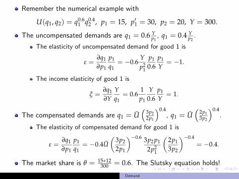
Remember the numerical example with

U(q1, q2) = q0.61 q0.4

2 , p1 = 15, p01 = 30, p2 = 20, Y = 300.

The uncompensated demands are q1 = 0.6 Yp1, q1 = 0.4 Y

p2.

The elasticity of uncompensated demand for good 1 is

ε =∂q1

∂p1

p1

q1= �0.6

Yp2

1

p1

0.6p1

Y= �1.

The income elasticity of good 1 is

ξ =∂q1

∂YYq1= 0.6

1p1

Y0.6

p1

Y= 1.

The compensated demands are q1 = U�

3p22p1

�0.4, q1 = U

�2p13p2

�0.4.

The elasticity of compensated demand for good 1 is

ε =∂q1

∂p1

p1

q1= �0.4U

�3p2

2p1

��0.6 3p2 p1

2p21

�2p1

3p2

��0.4= �0.4.

The market share is θ = 15�12300 = 0.6. The Slutsky equation holds!

Demand