Lecture Note: Social (Non-Market) Interactions

David AutorMIT 14.663 Spring 2009

May 12, 2009

1

1 Non-Market Interactions

Non-market interactions are interactions among individuals that are not regulated by the price

mechanism. They are a particular form of externality. Schelling is the intellectual father of this

branch of research. It has come some ways since Schelling, but perhaps not as far as one would

have anticipated.

1.1 The �social multiplier�

The social multiplier is a well-worn term, so you should be familiar with it. Let S equal the

level of social capital. We don�t need to de�ne what social capital is for now; we are only

concerned with what it does. Assume for the moment that everyone takes S as given (S = S0).

Individuals have the utility function:

U = U (x; y;S) :

Let y be the numeraire good and I be income. Agents maximize utility subject to

I = pxx+ y;

leading to the standard condition:UxUy= px:

How does a rise in S a¤ect demand for x? It depends on the relative complementarity of S

to y and x: UxS; UyS: So, rewriting the above condition:

Ux = pxUy:

If UxS > pxUyS, then consumption of x will increase and consumption of y will fall with a rise

in S: So,

Sign�dx

dS

�= Sign hUxS � pxUySi :

Notice that this model does not assume that an increase in �social capital�increases utility;

it�s possible that US < 0. What matters is how social capital changes the relative value of

other economic choices. For example if S is drug consumption by one�s peers, x is own drug

2

consumption, and y is all other goods, it�s plausible that a rise in S would raise own consumption

of x and lower utility.

Let�s assume that social capital of the peer group is simply equal to the average x of its

members:

S = X =1

N

Pj

xj:

Assume that N is large so no individual signi�cantly a¤ects S: Each member of the group

maximizes utility by choosing x taking S as a given.

The demand function for each individual is:

xj = dj�ej; p; S = X

�; where j = 1; 2; :::; N:

ej is an idiosyncratic taste variable and X is the level of social capital assumed by j when

choosing xj: So,

X =

Pdj (ej; p;X)

N=

Pxj

N; or X = F

�e1; e2; :::; en; p

�:

If S and x are strong complements, then person-level idiosyncratic taste shocks have little

e¤ect on person level-demand because S cannot be adjusted simultaneously by the individual.

Thus, each individual is heavily in�uenced by social capital.

However, if a shock hits all participants simultaneously, the cumulative e¤ect of individual

choices on social capital may matter greatly. One such shock is a change in p:

dS

dp=dX

dp=

Pdxj=dp

N=

P@xj=@p

N+

P(@xj=@S)� (dS=dp)

N:

Rearranging:

dS

dp

�1� 1

N

P�@xj=@S

��=

1

N

P@xj=@p;

dS

dp=

1N

P@xj=@p

1�m ; where m = (1=N)P@xj=@S:

Here m is the famed social multiplier. The larger is m; the more a common shock to individual

demands raises aggregate demand by more than could be predicted exclusively by summing

individual demand functions.

3

This is kind of a nice insight: an equilibrium that is locally stable, with well-behaved demand

curves at the individual level, can behave in a very non-standard fashion if a shock (such as

a price drop) causes a simultaneous change in demands of many participants at once. Even

though each participant has standard preferences holding other participants�behavior constant,

the spillover from the consumption of each consumer to the preference of others can make the

system highly reactive to common shocks.

1.2 Becker-Murphy fad model (see also Becker restaurant paper, 1991)

Write the aggregate demand for a good as:

Q = D (p; Z;Q) , with Dp < 0 and DQ > 0;

and Z are other demand shifters. Holding all else constant, demand is decreasing in price. But

the assumption that DQ > 0 means that demand for the good increases when its popularity

rises (i.e., more people are consuming it).

Using the notation above,dQ

dp=

Dp

1�m:

The sign of this is ambiguous. Assume there exists a Q� where m = 1 for Q = Q�, m > 1 for

Q > Q� and m < 1 for Q > Q�: This gives rise an unstable demand curve. Demand is upward

sloping below Q�; downward sloping above Q�; and reaches an in�ection point at Q�:

See Figure 9.1 of Becker-Murphy. If the �market-clearing�price is on the upward sloping

section of the demand curve (Q < Q�), the �rm can raise p further without incurring a loss

in demand (in fact, just the opposite). If output is capped, then it will clearly make sense

to raise p to increase quantity towards Q�. This will create excess demand, but the pro�t

earned per each unit sold will be higher (assuming that the rationing process is not costly).

If the monopolist raises the price all the way to where Q = Q�, demand becomes extremely

unstable. A tiny shock in either direction could cause demand to fall precipitously. Thus, it

might be pro�t-maximizing to a choose p so that Q is slightly less than Q�: (This is one possible

explanation for why fads� like popular restaurants� are so �eeting.)

4

In interpreting cases where m > 1, it is important to observe that the positive slope of the

demand function does not mean that individual level demand rises as the price of the good

increases. Rather that each agent�s willingness to pay for the good increases as other agents

also consume the good (or express the desire to do so).

2 Evidence: Duflo and Saez (2003)

There is precious little credible work on social interactions. Du�o and Saez is an excellent

example of a randomized experiment that is able to identify social interactions� though as they

point out, the experiment is still under-identi�ed in that only half of the behavioral parameters

of interest can be estimated.

� Every employee can contribute to a Tax Deferred Account (TDA) up to $10,500.

� Bene�ts fair annually. Noti�cation one month before.

� Participation rate is 34%, which is low relative to other universities.

� Encouragement design: o¤ering a randomly chosen subset of employees a small amount

of money for attending the fair.

� Randomization is at two levels: at level of department and at level of individuals in the

department.

� Thus, two treatments: receiving a letter; being in a department where someone receives a

letter. The treatment groups are: 11 equals receiving a letter and being in a department

that someone received a letter (these have to go together); 10 not receiving a letter but

being in a treated department; 00 no letter in department.

� Outcomes are: fair attendance, TDA participation after 4.5 months, TDA participation

after 11 months.

� Table I makes it clear that something happened as a result of treatment. Fair attendance

was 5 times as high among those who received the letter (group 11) as those who did

not, and it was 3 times as high among those in departments where someone else received

5

a letter (group 11). Eleven months after the intervention, participation in the TDA was

somewhat higher for both group 10 and group 11, though they do not appear di¤erent

from one another.

� Table II presents reduced form estimates:

fij = �1 + �1Dj + "ij;

Yij = �2 + �2Dj + !ij;

where D is a dummy variable for being a member of a treated department.

� Notice the puzzle here. The D treatment clearly raises the probability of fair attendance

and TDA enrollment. Those who received letters were more likely to attend the fair but

less likely to enroll than coworkers in their departments who did not receive a letter.

2.1 Interpretation

There is no entirely unambiguous way to interpret theses results. Assumptions are needed.

� Consider the following equation for TDA participation:

yij = �+ ifij + �Dj + uij;

where Dj is a dummy indicating that the department was treated and f is an indicator

equal to one if the i attended the fair. The fact that is indexed by i means that this is

a random coe¢ cients model.

� There are three treatment groups, corresponding to the combination of D and L received:

fD;Lg 2 f00; 10; 11g. Note that there is no 01 group since if an individual received the

letter, his department is also treated by de�nition.

� De�ne potential outcomes for fair attendance as f (11) ; f (10) ; f (00)

� Consider the following identi�cation assumptions for fair attendance:

6

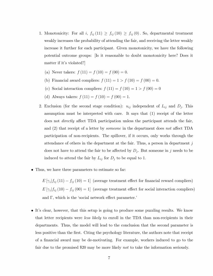
1. Monotonicity: For all i, fij (11) � fij (10) � fij (0) : So, departmental treatment

weakly increases the probability of attending the fair, and receiving the letter weakly

increase it further for each participant. Given monotonicity, we have the following

potential outcome groups: [Is it reasonable to doubt monotonicity here? Does it

matter if it�s violated?]

(a) Never takers: f (11) = f (10) = f (00) = 0.

(b) Financial award compliers: f (11) = 1 > f (10) = f (00) = 0.

(c) Social interaction compliers: f (11) = f (10) = 1 > f (00) = 0

(d) Always takers: f (11) = f (10) = f (00) = 1.

2. Exclusion (for the second stage condition): uij independent of Lij and Dj: This

assumption must be interpreted with care. It says that (1) receipt of the letter

does not directly a¤ect TDA participation unless the participant attends the fair,

and (2) that receipt of a letter by someone in the department does not a¤ect TDA

participation of non-recipients. The spillover, if it occurs, only works through the

attendance of others in the department at the fair. Thus, a person in department j

does not have to attend the fair to be a¤ected by Dj. But someone in j needs to be

induced to attend the fair by Lij for Dj to be equal to 1:

� Thus, we have three parameters to estimate so far:

E [ ijfij (11)� fij (10) = 1] (average treatment e¤ect for �nancial reward compliers)

E [ ijfij (10)� fij (00) = 1] (average treatment e¤ect for social interaction compliers)

and �, which is the �social network e¤ect parameter.�

� It�s clear, however, that this setup is going to produce some puzzling results. We know

that letter recipients were less likely to enroll in the TDA than non-recipients in their

departments. Thus, the model will lead to the conclusion that the second parameter is

less positive than the �rst. Citing the psychology literature, the authors note that receipt

of a �nancial award may be de-motivating. For example, workers induced to go to the

fair due to the promised $20 may be more likely not to take the information seriously.

7

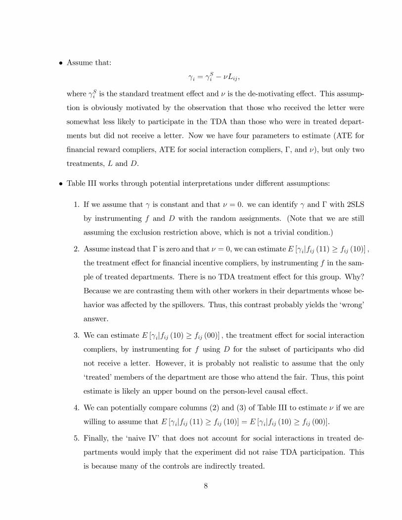
� Assume that:

i = Si � �Lij,

where Si is the standard treatment e¤ect and � is the de-motivating e¤ect. This assump-

tion is obviously motivated by the observation that those who received the letter were

somewhat less likely to participate in the TDA than those who were in treated depart-

ments but did not receive a letter. Now we have four parameters to estimate (ATE for

�nancial reward compliers, ATE for social interaction compliers, �, and �), but only two

treatments, L and D.

� Table III works through potential interpretations under di¤erent assumptions:

1. If we assume that is constant and that � = 0. we can identify and � with 2SLS

by instrumenting f and D with the random assignments. (Note that we are still

assuming the exclusion restriction above, which is not a trivial condition.)

2. Assume instead that � is zero and that � = 0, we can estimateE [ ijfij (11) � fij (10)] ;

the treatment e¤ect for �nancial incentive compliers, by instrumenting f in the sam-

ple of treated departments. There is no TDA treatment e¤ect for this group. Why?

Because we are contrasting them with other workers in their departments whose be-

havior was a¤ected by the spillovers. Thus, this contrast probably yields the �wrong�

answer.

3. We can estimate E [ ijfij (10) � fij (00)] ; the treatment e¤ect for social interaction

compliers, by instrumenting for f using D for the subset of participants who did

not receive a letter. However, it is probably not realistic to assume that the only

�treated�members of the department are those who attend the fair. Thus, this point

estimate is likely an upper bound on the person-level causal e¤ect.

4. We can potentially compare columns (2) and (3) of Table III to estimate � if we are

willing to assume that E [ ijfij (11) � fij (10)] = E [ ijfij (10) � fij (00)].

5. Finally, the �naive IV�that does not account for social interactions in treated de-

partments would imply that the experiment did not raise TDA participation. This

is because many of the controls are indirectly treated.

8

Conclusions: (1) It�s hard to do this type of exercise well; (2) This is a successful e¤ort.

3 Montgomery, 1991: Social Networks and Labor Market Outcomes

Most people �nd jobs through social networks. Many employers believe that employee referrals

are a useful device for screening job applicants. The 1991 Montgomery paper o¤ers an explana-

tion for why well-connected workers may fare better than poorly connected workers, and why

�rms hiring through referral might earn higher pro�ts. This is widely considered a seminal

paper. I am not aware of empirical research that directly builds from this model, however.

3.1 Workers

� There are two periods.

� Each worker lives for one period.

� There are two types of workers, both equally populous: H and L:

� High ability workers produce 1 and low ability workers produce 0:

� Employers cannot observe worker ability prior to hiring.

� There are no output-contingent contracts. (As Montgomery notes, if such contracts were

readily feasible, the entire issue of screening and the considerable e¤ort that employers

spend on worker selection would seemingly be pointless.)

3.2 Firms

� Each �rm may employ up to 1 worker.

� Pro�t equals productivity minus the wage.

� Product price of 1 is exogenous determined.

� Firms must set wages prior to learning the productivity of their workers.

� They do observe their own worker�s type prior to the start of the second period (of course,

that worker is about to die).

9

� There is free entry

3.3 Social structure

� Each period 1 worker knows (is �tied�to) at most one period 2 worker. Speci�cally, the

probability of such a tie is � 2 [0; 1]. So, if there are 2N workers in period 1, there will

be 2�N ties.

� Ties are drawn with replacement. Thus, although a period 1 worker can only have one

tie, a period 2 worker can have any non-negative number of ties. Hence, the distribution

of ties in period 2 is binomial with mean � and variance � (1� �).

3.4 Two observations

1. Hiring a worker in period 1 has an associated option value. This arises from the fact that

the period 1 worker may be type H and may have a tie to another type H worker (the

joint probability being 12��).

2. Intuition should suggest that this network mechanism could give rise to adverse selection.

� An employer who observes that she has hired a type H worker in period 1 who has

a network tie (joint probability 12�) faces probability � > 1=2 of receiving a referral

to another type H worker.

� This conditional probability of � is better than the employer could do by chance in

period 1 (the unconditional probability being 1=2).

� This conditional probability is better still than the employer could obtain by chance

in period 2. This is because, as will be shown, type H period 2 workers will be more

likely than type L workers to receive o¤ers via referrals (and to accept those o¤ers).

� Consequently, the pool of workers on the open market (i.e., those not hired through

referrals) will be adversely selected. The workers available on the period 2 open

market will have Pr (H) < 12< �.

10

3.5 Main proposition

The solution to the model is non-trivial and enlightening. Montgomery starts with the following

proposition, which is initially assumed and subsequently proved:

Proposition 1 A �rm makes a referral o¤er i¤ it employs a type H worker in period 1.

Referral wage o¤ers are dispersed over the interval [wM2; �wR].

In this proposition, wM2 is the market wage in period 2.

3.6 Structure of the proof

The structure of the proof is complex and features many twists and turns. Here�s the roadmap:

1. We �rst solve the worker�s problem

(a) Calculate the structure of ties (i.e., how many ties a worker can expect to have)

(b) Calculate the probability that an o¤er is accepted by a period two H worker

2. Calculate the market wage for workers who receive no referral.

3. Given the market wage and the expected productivity of referrals, calculate �rms�referral

wage o¤ers (i.e., the o¤ers that they make if they hire an H worker in period 1 and that

worker has a network tie). Given the proposition above:

(a) Show that o¤ering WM2 is one feasible strategy

(b) Calculate �WR and show that o¤ering a higher wage than �WR is not an equilibrium

strategy

(c) Argue that wage o¤ers on the interval�WM2; �WR

�must all be equally good

4. Prove that �rms who have hired L workers hire on the open market (i.e., not through

referrals)

5. Calculate period one wages by backward induction

6. Re�ect on our accomplishment

11

3.7 The worker�s problem

3.7.1 The structure of ties

� The distribution of ties in period 2 is binomial with mean � and variance � (1� �). The

way to think about the problem is that there are a total of 2N draws with replacement

from the urn of period 2 workers, where each draw selects one period 2 worker with

probability � .

� The likelihood that a given period 2 worker receives exactly k ties is:

Pr [ki = k] =�2Nk

�� �2N

�k �1� �

2N

�2N�k;

where �2Nk

�=

2N !

k! (2N � k)! :

� Now assume that ties exhibit homophily. Conditional on a tie existing, the probability

that the period 2 worker is of the same type as the period 1 worker to which he is tied is

� > 1=2.

� Thus, if a �rm observes that its period 1 worker is type H (which occurs in N cases),

there is a probability � that this worker has a tie, and a probability �� that the worker

has a tie to a period 2 worker of type H.

� The probability that a given period 2 worker of type H has k ties to period 1 workers

of type H is:

Pr [ki = k] =(N � k)!k! (N � k)!

���N

�k �1� ��

N

�N�k:

Note that the 2N term has become an N term because there are only N type H workers

in the total population of 2N workers.

3.7.2 The probability that a period two H worker accepts a wage offer

� Consider a given typeH worker in period 2: Assuming the proposition holds, so all referral

o¤ers exceed the market wage. The probability that H accepts a given referral wage o¤er

12

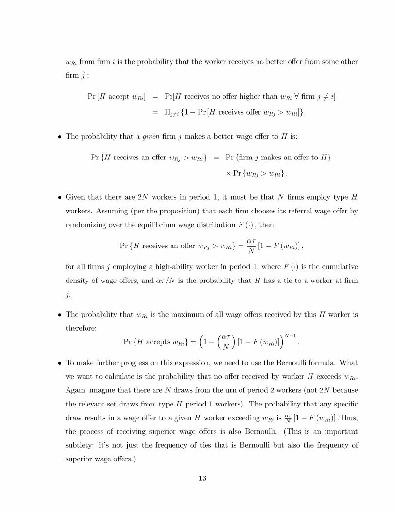
wRi from �rm i is the probability that the worker receives no better o¤er from some other

�rm _j :

Pr [H accept wRi] = Pr[H receives no o¤er higher than wRi 8 �rm j 6= i]

= �j 6=i f1� Pr [H receives o¤er wRj > wRi]g :

� The probability that a given �rm j makes a better wage o¤er to H is:

Pr fH receives an o¤er wRj > wRig = Pr f�rm j makes an o¤er to Hg

�Pr fwRj > wRig :

� Given that there are 2N workers in period 1; it must be that N �rms employ type H

workers. Assuming (per the proposition) that each �rm chooses its referral wage o¤er by

randomizing over the equilibrium wage distribution F (�) ; then

Pr fH receives an o¤er wRj > wRig =��

N[1� F (wRi)] ;

for all �rms j employing a high-ability worker in period 1, where F (�) is the cumulative

density of wage o¤ers, and ��=N is the probability that H has a tie to a worker at �rm

j.

� The probability that wRi is the maximum of all wage o¤ers received by this H worker is

therefore:

Pr fH accepts wRig =�1�

���N

�[1� F (wRi)]

�N�1:

� To make further progress on this expression, we need to use the Bernoulli formula. What

we want to calculate is the probability that no o¤er received by worker H exceeds wRi.

Again, imagine that there are N draws from the urn of period 2 workers (not 2N because

the relevant set draws from type H period 1 workers). The probability that any speci�c

draw results in a wage o¤er to a given H worker exceeding wRi is ��N [1� F (wRi)] :Thus,

the process of receiving superior wage o¤ers is also Bernoulli. (This is an important

subtlety: it�s not just the frequency of ties that is Bernoulli but also the frequency of

superior wage o¤ers.)

13

� The probability that a period two H worker receives exactly k superior wage o¤ers given

wRi is (we use N � 1 because one o¤er is already in hand):

Pr [ki = kjwRi] =(N � 1� k)!k! (N � 1� k)!

��� [1� F (wRi)]

N

�k �1� �� [1� F (wRi)]

N

�N�1�k:

� We need to calculate the probability that an H worker receives zero superior wage o¤ers.

Why? Because a worker who receives zero superior o¤ers will take the o¤er that is in

hand

Pr [ki = 0jwRi] =�1� �� [1� F (wRi)]

N

�N�1:

3.7.3 The tricky part

� This expression is very close to the following limit:

limn!1

�1� �� [1� F (wRi)]

n

�n=

1

e�� [1�F (wRi)]= e��� [1�F (wRi)]:

� More familiar:

limn!1

�1� 1

n

�n=1

e;

and

limn!1

�1 +

1

n

�n= e:

� So, putting pieces together. The probability that H accepts �rm i0s o¤er is:

Pr [H accepts wRi] = e��� [1�F (wRi)];

and similarly, the probability that L accepts �rm i0s o¤er (remember, period 2 workers

are also tied to period 1 H workers with probability (1� �) �) is:

Pr [L accepts wRi] = e�(1��)� [1�F (wRi)]:

3.8 The firm�s problem

3.8.1 Period 2 market (non-referral) wages

� What should a �rm o¤er to a period two worker who is in the open market (i.e., not hired

by through a referral)?

14

� Since referral wage o¤ers always dominate market wage o¤ers, the probability that a type

H worker enters the market in period 2 is equal to the probability of receiving no wage

o¤ers:

Pr fMarket jHg = e��� :

and for type L workers, this probability is:

Pr fMarketjLg = e�(1��)� :

� This brings us to the adverse selection problem. The o¤er wage (equal to expected

productivity) of period 2 workers on the market is:

wM2 = Pr fHjMarketg =e���

e��� + e�(1��)�<1

2:

Period 2 market workers are therefore adversely selected.

� Moreover:@wM2

@�< 0;

@wM2

@�< 0:

The adverse selection problem becomes more severe the denser are social networks (�+)

and the greater is the degree of homophily (�+).

3.8.2 Period 2 referral wages

� Consider the expected period 2 pro�t of a �rm employing a type H worker in period 1

and setting a referral wage of wR:

E�H(wR) = Pr [Type H referral hiredjwR] � (1� wR)

+Pr [Type L referral hiredjwR] � (�wR)

+Pr [No referral hiredjwR] � 0;

where in this expression we use the fact that hiring in the outside market must have

expected pro�t of zero (i.e., it�s a competitive situation� unlike referrals where markets

are �thin�).

15

� Conditional on hiring a type H worker in period 1, the probability of hiring a period two

H worker with o¤er wage wR is:

Pr [Type H referral hiredjwR] = ��e��� [1�F (wR)]:

Similarly,

Pr [Type L referral hiredjwR] = (1� �) �e�(1��)� [1�F (wR)]:

So,

E�H(wR) = ��e��� [1�F (wR)] � (1� wR) + (1� �) �e�(1��)� [1�F (wR)] � (�wR) :

� In equilibrium, this pro�t level must be robust to deviations.

3.8.3 The lower-bound wage

� A �rm could simply o¤er the market wage wM2 (or wM2 + ") to a referral (a �low-ball�

strategy), and that referral will be accepted if the worker has received no other o¤ers�

which will occur with positive probability, even in an in�nitely large workforce, given that

there are fewer than half as many referral o¤ers as workers.

� Given that H worker is receiving a referral o¤er, what is the probability that he receives

no other?

Pr [ki = 1jH; ki � 1] =(N � 1� k)!k! (N � 1� k)!

���N

�k �1� ��

N

�N�k�1=

�1� ��

N

�N�1� e���

� Similarly, for an L worker:

Pr ki = 1jL; ki � 1 � e�(1��)�

16

� So, the pro�tability of the low-ball strategy is:

E�H(wM2) = ��e��� (1� wM2) + (1� �) �e�(1��)� (�wM2)

= ��e����1� e���

e��� + e�(1��)�

�+ (1� �) �e�(1��)�

�� e���

e��� + e�(1��)�

�=

���e��� � ��e�2��

e��� + e�(1��)�

�+ (�� 1)

��e�(1��)����

e��� + e�(1��)�

�=

��e����e��� + e�(1��)�

�� ��e�2��

e��� + e�(1��)�+

(�� 1) �e��e��� + e�(1��)�

=��e��

e��� + e�(1��)�+

(�� 1) �e��e��� + e�(1��)�

=(2�� 1) �

e���+� + e�(1��)�+�

=(2�� 1) �e�� + e(1��)�

:

� Call this pro�t level c:

c (�; �) � (2�� 1) �e�� + e(1��)�

> 0;

which is positive since � > 1=2. By implication, �rms who hire a type H worker in period

1 earn a positive expected pro�t in period 2: Moreover,

c� > 0; c� > 0:

3.8.4 The upper-bound wage

� Clearly, in equilibrium, �rms with a type H worker must receive c (�; �) from either

making an o¤er of wR or making an o¤er of wM2: So, it must be the case that for all wR :

c (�; �) = ��e��� [1�F (wR)] � (1� wR)

+ (1� �) �e�(1��)� [1�F (wR)] � (�wR)

8wR 2 [wM2; �wR]

Montgomery o¤ers the interpretation that either �rms randomize their o¤ers over the

entire distribution or else a fraction f (wR) of �rms o¤ers each wage for sure. Montgomery

claims (and I, for one, believe him) that this expression does not have a closed form

solution.

17

� However, we know that if a �rm o¤ers �wR; it hires the referred worker for sure (conditional

on having a H worker with a tie). Thus, we can solve for �wR

(2�� 1) �e�� + e(1��)�

= �� (1� �wR) + (1� �) � (� �wR)

(2�� 1) �e�� + e(1��)�

= �� � �wR � �wR + � �wR

�wR = �� (2�� 1) =�e�� + e(1��)�

��wR (�; �) = �� c (�; �) =� :

� One can easily show that @ �wR=@� > 0; @ �wR=@� > 0: That is, the maximum referral wage

o¤er is also increasing in network density and homophily.

� Summing up, the expected period 2 pro�t from hiring a type H worker is:

E�H = (�� �wR) � ;

which is also increasing in � and � :

3.9 Do firms who have hired L workers hire only on the open market?

� We have established that �rms holding type H workers who have ties make o¤ers on the

interval [wM2; �wR] : Lower o¤ers are not accepted and higher o¤ers do not increase the

probability of attracting a worker.

� We now need to prove that �rms hiring type L workers in period 1 will hire through the

market.

� Imagine a �rm deviated from the equilibrium by making a referral o¤er wM2 < wR < �wR

via its type L worker:

E�L (wR) = (1� �) �e��� [1�F (wR)] � (1� wR) + ��e�(1��)� [1�F (wR)] � (�wR) :

� It is immediately apparent that

E�L (wR)

@wR<E�H (wR)

@wR:

18

This follows because any action that increases the chance of the o¤er being accepted

increases the winner�s curse (since odds are better than 50% that the worker will be type

L). And we know by construction that

@E�H (wR) =@wR = 0 8 wR 2 [wM2; �wR] :

Thus,@E�L (wR)

@wR< 0

.

� By implication, E�L (wR) is maximized at wR = wM2: But we can show that this expec-

tation is negative using the formula derived above for wM2:

E�L (wM2) = (1� �) �e��� [1�F (wR)] � (1� wM2) + ��e�(1��)� [1�F (wR)] � (�wM2)

= (1� �) �e��� [1�F (wR)] ��1� e���

e��� + e�(1��)�

�+��e�(1��)� [1�F (wR)] �

�� e���

e��� + e�(1��)�

�=

(1� 2�) e��e��� + e�(1��)�

:

This expression is negative since � > 1=2: Thus, a �rm employing a L worker in period

1 will o¤er the market wage in period 2: It will not use referrals.

3.10 Calculating period 1 wage

� Finally, consider the period 1 wage (where types are not known). This wage incorporates

both the expectation of period 1 productivity and the option value of a period 2 referral:

wM1 (�; �) =1

2+1

2c (�; �) =

1

2[1 + c (�; �)] :

Given prior results on c (�) ; this implies that wM1 is increasing in � and � : That�s an

interesting result in that low-ability workers bene�t from the uncertainty in period 1 but

are harmed by the adverse selection in period 2:

19

3.11 Main results: Summary (AKA, reflect on our accomplishment)

The key results of the model are:

1. In equilibrium, each worker�s wage is determined not by his actual skill but by the number

and types of social ties he holds (though of course these are not independent of worker

skill). Period 2 workers with more ties to high-ability Period 1 workers receive more

referrals and thus higher expected wages. Workers with no ties to high ability workers

�nd employment on the open market, which is a­ icted with adverse selection. (Thus,

It�s who you know, not what you do.)

2. In equilibrium, workers obtained through referrals are of higher quality. So, it is rational

for �rms to prefer referrals, and these referrals to generate rents (which are dissipated

into the labor market in period 1 in the form of option value payments).

3. Both � and � have similar e¤ects in the model (and it�s not really clear that these

parameters need to be conceptually distinct). An increase in either raises the top wage

( �wR) and lowers the bottom wage (wM2) and also raises the period 1 wage (wM1).

4. One model extension in which � and � might di¤er is in a setting where there are di¤erent

groups that are intrinsically of equal ability and have similar homophily along the lines

of ability but one group has a better network (�+) than the other. So, take the case of

Blacks and Whites. If Whites have a better network, even with equal ability, the option

value of hiring Whites is greater than that of hiring Blacks in period 1, even if the White

network advantage stems from their connection to type H Blacks. Thus, network density

redistributes income from the those who are referred to those doing the referring. Of

course, referred workers also bene�t. The more o¤ers a period 2 worker receives, the

higher his wage. (Remember that the accepted wage is the highest wage o¤ered, and each

o¤er is a random variable. So a larger number of o¤ers increases the expected accepted

wage):

5. If there is a complementarity between ability and the production technology (such that

�rms would use one technology if they could be reasonably con�dent of getting type H

20

workers and another if they could not), then an increase in � might improve productive

e¢ ciency but also increase inequality. This idea is the essence of the model in Acemoglu

1999 in the AER.

This is a path-breaking paper that continues to be widely cited. What is most thought-

provoking about it is: (a) it suggests a non-market mechanism that could a¤ect economic

outcomes in a competitive environment (assumption: there is not a market for social ties); (b)

it provides the insight that the option value of networks accrues (at least in part) to those at

the top of the network (referring) rather than exclusively those being referred.

4 The effect of Social Networks on Employment and Inequality:Calvo-Armengol and Jackson (2004)

The 2004 paper by Calvo-Armengol and Jackson presents a distinctly di¤erent way of modeling

social networks and their potential impact on employment. In their model, there are no prices,

no wages, no adverse selection and no individual heterogeneity� so the market mechanism is

quite impoverished relative to Montgomery (1991). However, the network structure is richer.

In particular, it has a topological aspect wherein which workers are connected to one another

via multiple nodes. The model appears to capture the seemingly important phenomenon that

individuals are tied to one another both directly (as in � in Montgomery) and indirectly through

other acquaintances. This extremely sparse model gives rise to surprisingly rich interactions.

4.1 Model basics

� There are n agents.

� Time involves in discrete periods indexed by t

� The vector st describes the employment status of all agents at time t:

� If agent i is employed at the end of period t, then sit = 1; and if unemployed, sit = 0.

� A period t begins with some agents employed and others not, described by the status st�1from the last period.

21

� Next, information about jobs opening arrives.

� In each period, any given agent hears about a new job opening with probability a 2 (0; 1).

� If the agent is unemployed, she takes the job.

� If the agent is employed, she passes the information to someone in her immediate network

who is unemployed.

4.2 Network structure

� Any two agents either know one another or not.

� Information only �ows between agents who know each other.

� A graph g summarizes the links of all agents, where gij = 1 indicates that i and j have a

link.

� Links are re�exive: gij = gji:

� If an agent hears about a job and is employed, she passes the information to another

randomly chosen linked agent who is unemployed.

� If all of her linked agents are employed, the information is lost.

� Thus, the probability that agent i learns about a job and that this job is taken by agent

j is described by pis (s) :

pis (s) =

8>><>>:a if si = 0 and i = j

a

Pk:sk=0

gik

!�1if si = 1, sj = 0, and gij = 1

0 otherwise

:

� At the end of a period, each employed worker loses her job with probability b:

Some notes:

22

1. If there were no network structure, this setup be a simple Markov process with transition

probabilities Pr (U ! E) = a, Pr (E ! U) = b, and steady state employment probability

of a= (a+ b). [In steady state E�b = U�a: So, EU= a

b; and the employment to population

rate is E= (E + U) = a= (a+ b).

2. There is no communication beyond one node in the graph. That is, a job referral does

not pass from agent i to j to k:This means that any network e¤ects beyond immediate

acquaintances are indirect.

3. If we think about two agents each linked to a third agent, these two agents are competitors

for job information in the short run. But in the longer run, they help to keep one

another employed indirectly. In particular, if the shared friend becomes unemployed,

then each acquaintance potentially helps to re-employ the shared friend. This bene�ts

the other acquaintance because if the shared friend is re-employed, he potentially helps

the acquaintances should they become unemployed.

4.3 Some basics

The paper is chock-full of thought-provoking examples.

� Figure 2 shows that although agents are competitors for the job info possessed by a mutual

friend, there will still tend to be a positive correlation in employment rates between agents

with a mutual friend.

� A formal proposition shows that under �ne enough time subdivisions (where a and b are

divided by some common T , so the periods become extremely short), the unique steady-

state long-run distribution on employment is such that the employment statuses of any

path-connected agents are positively correlated (where path-connectedness can mean a

direct or indirect connection).

� Moreover, the positive correlation holds across any arbitrary time span. That is, agent

i0s employment status at time t is correlated with agent j0s status at time t0 for all t and

t0:

23

4.4 Duration dependence

� Suppose that a = 0:1 and b = 0:015: Given that a person has been unemployed for at

least each of the last X periods. What is the probability that she will �nd employment

this period?

� Figure 6 illustrates. Notice the negative duration dependence of re-employment. The

longer an agent is unemployed, the lower his re-employment probability. Yet we know

there is no heterogeneity among agents, and there is no change in aggregate labor market

conditions. What�s going on?

� The longer that i has been unemployed, the higher the expectation that i0s connections

and path connections are themselves unemployed. This makes it more likely that i0s

connections will take jobs that arrive rather than passing them down.

� To clarify, this is not a causal e¤ect of i being unemployed. Rather, i having remained

unemployed for some time provides information about the poor employment status of his

connections. Thus, our expectation of his exit hazard falls.

� This observation interesting because it suggests that individuals may experience time-

varying serially correlated reemployment probabilities that are explained by network sta-

tus but not otherwise due to either person-level characteristics or the aggregate state of

the economy. So, if my friends lose a job due a plant closing, I may be less likely to �nd

re-employment conditional on job loss not because fewer jobs are available but because

I�m less likely to hear about them.

4.5 Dynamics

� Given the network externalities in the model, it should be clear that the state of aggregate

employment can cycle. If the network gets close to full employment, unemployed agents

become ever more likely to �nd jobs. If employment falls due to a set of chance events,

each newly unemployed worker also becomes less likely to �nd reemployment. This leads

to booms and busts.

24

� Nevertheless, the sharing of information about jobs means that more o¤ers get used (fewer

get lost) than in a network with no connections. So, aggregate employment is likely to

remain higher in a networked than non-networked market. See Figure 7.

4.6 Dropping out and contagion

Perhaps the most interesting part of the article in my mind is the section on labor market

dropouts. As constructed so far, the steady states of a network does not depend on initial

conditions. That is, whether all nodes are initially employed or unemployed, the model will

move towards the same average level of employment. If the model is expanded to allow labor

market drop-out, however, the dynamics get richer.

In particular, CJ add a �drop out�option as an absorbing state of the model. Agents face a

present value of costs ci � 0 of remaining in the market. The outside option is zero. So an agent

will only remain in the LF if the discounted expected value of wages exceeds ci: The per-period

wage will be �xed at 1: A key assumption is that once an agent drops out, he no longer passes

along job referrals to linked agents and yet remains in the network. Thus, his a signals are

e¤ectively lost. Moreover, it is assumed for simplicity that the dropout�s connected agents still

send referrals to him (and thus they are squandered). [Without this assumption, the network

structure would e¤ectively change when an agent dropped out, which would complicate things

greatly.]

Clearly, dropout probabilities will be rising in costs and declining in wages. More inter-

estingly, an agent�s dropout probability will depend on her network. The better a person�s

network, the greater the re-employment hazard following job loss, and thus the greater the

discounted expected future value of earnings.

Most interestingly, agents dropout decisions can have contagion e¤ects because one agent�s

exit weakens the network for each of her path-dependent agents. Accordingly, decisions to

remain in the labor force are strategic complements� the more participants remain in, the more

advantageous it is for a given agent to remain. The dropout game is therefore supermodular (in

calculus terms, positive cross-partials for all components). This means the game has a maximal

equilibrium in pure strategies where the set of agents staying in the game is maximized (though

25

the speci�c identities of the agents could change across equilibria or points in time). Drop-

outs can have negative contagion e¤ects due to the strategic complementarities among agents�

actions.

To simulate this setting, CJ set the cost ci uniformly on [0:8; 1] and �x the wage at 1: They

assume a complete network� every agent is linked. The discount factor is 0:9 and the transition

probabilities are a = 0:1 and b = 0:015:

To calculate contagion, they �rst calculate drop out rates that would occur if every agent

assumed that every other agent were staying in the market. Then they calculate how many

agents drop out in equilibrium (calculated by simulation). The di¤erence between these two is

the estimated contagion e¤ect.

See Tables 2 and 3. Several things are interesting about these results:

� Contagion e¤ects are substantial in some cases.

� With a very large number of nodes in a fully connected network, the contagion e¤ect

becomes negligible. This is because any one person�s dropout decision is inconsequential

for all other agents.

� Contagion e¤ects are more important when workers start unemployed than employed�

presumably because more workers drop out immediately, leading to further dropout.

Thus, the network is state dependent in that the starting state in�uences the long-run

equilibrium. A proposition demonstrates this observation formally. If the starting state

in two identical networks is person-by-person (weakly) higher in one network than the

other, then the network that starts initially higher has higher steady-state employment,

and this is true for all agents in any component of the network for which equilibrium

drop-out decisions di¤er across the two groups.

� A �nal observation is that holding the equilibrium unemployment rate constant U =

a= (a+ b), a higher rate of turnover (higher b) induces a greater level of dropout. The

reason is that the likelihood that an agent and his linked agents are simultaneously un-

employed is higher in the setting where job destruction is more frequent. Thus, they are

more likely to be in competition for job arrivals, which leads to an increase in dropout.

26

4.7 Substantive conclusions from CJ

I personally �nd it di¢ cult to know how much stock to place in this thought-provoking paper.

The stylized takeaway for me is that there could be important externalities in job awareness,

leading to a dropout behavior that is contagious not due to peer imitation but simply due to

adverse information externalities. The concern for me is that the model is so stripped-down

that it�s hard to call it an economic model:

� There are no wages (or they are parametric).

� Labor demand is independent of supply� so, if fewer agents work, this does not increase

the arrival rate of o¤ers or reduce the job destruction rate of remaining workers.

� Network structure is exogenous and �xed.

� Agents are not maximizing anything in particular� except when calculating drop-out.

Thus, this model is very much in the style of a Sante Fe Institute computerized-automata

model: agents with a very limited repertoire of behavior are set loose in a simulated economic

environment and then we study the emergent properties of that environment. When you read

the Becker-Murphy (2000) volume on Social Economics, you will see that Becker-Murphy take

issue with this type of modeling (though obviously not with this paper). This type of model

will have to evolve considerably to make contact with more general economic models.

27