Embed Size (px)
Citation preview
Lecture Notes 1: Matrix AlgebraPart D: Similar Matrices and Diagonalization
Peter J. Hammond
minor revision 2019 September 16th
University of Warwick, EC9A0 Maths for Economists Peter J. Hammond 1 of 64
OutlineEigenvalues and Eigenvectors
Real CaseThe Complex CaseLinear Independence of Eigenvectors
Diagonalizing a General MatrixSimilar Matrices
Properties of Adjoint and Symmetric MatricesAn Adjoint Matrix has only Real EigenvaluesThe Spectrum of a Self-Adjoint Matrix
Diagonalizing a Symmetric MatrixOrthogonal MatricesOrthogonal ProjectionsRayleigh QuotientThe Spectral Theorem
Quadratic Forms and Their DefinitenessQuadratic FormsThe Eigenvalue Test of Definiteness
University of Warwick, EC9A0 Maths for Economists Peter J. Hammond 2 of 64
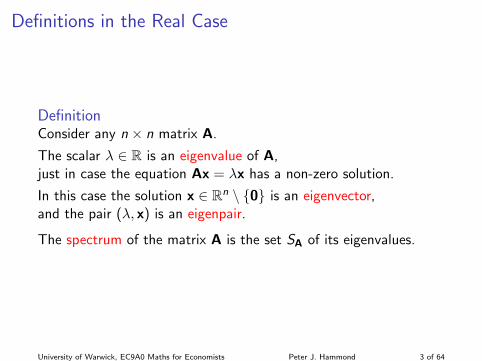
Definitions in the Real Case
DefinitionConsider any n × n matrix A.
The scalar λ ∈ R is an eigenvalue of A,just in case the equation Ax = λx has a non-zero solution.
In this case the solution x ∈ Rn \ {0} is an eigenvector,and the pair (λ, x) is an eigenpair.
The spectrum of the matrix A is the set SA of its eigenvalues.
University of Warwick, EC9A0 Maths for Economists Peter J. Hammond 3 of 64
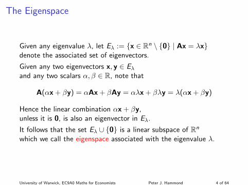
The Eigenspace
Given any eigenvalue λ, let Eλ := {x ∈ Rn \ {0} | Ax = λx}denote the associated set of eigenvectors.
Given any two eigenvectors x, y ∈ Eλ
and any two scalars α, β ∈ R, note that
A(αx + βy) = αAx + βAy = αλx + βλy = λ(αx + βy)
Hence the linear combination αx + βy,unless it is 0, is also an eigenvector in Eλ.
It follows that the set Eλ ∪ {0} is a linear subspace of Rn
which we call the eigenspace associated with the eigenvalue λ.
University of Warwick, EC9A0 Maths for Economists Peter J. Hammond 4 of 64
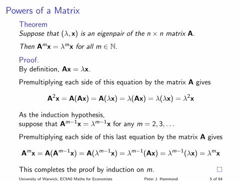
Powers of a Matrix
TheoremSuppose that (λ, x) is an eigenpair of the n × n matrix A.
Then Amx = λmx for all m ∈ N.
Proof.By definition, Ax = λx.
Premultiplying each side of this equation by the matrix A gives
A2x = A(Ax) = A(λx) = λ(Ax) = λ(λx) = λ2x
As the induction hypothesis,suppose that Am−1x = λm−1x for any m = 2, 3, . . .
Premultiplying each side of this last equation by the matrix A gives
Amx = A(Am−1x) = A(λm−1x) = λm−1(Ax) = λm−1(λx) = λmx
This completes the proof by induction on m.University of Warwick, EC9A0 Maths for Economists Peter J. Hammond 5 of 64
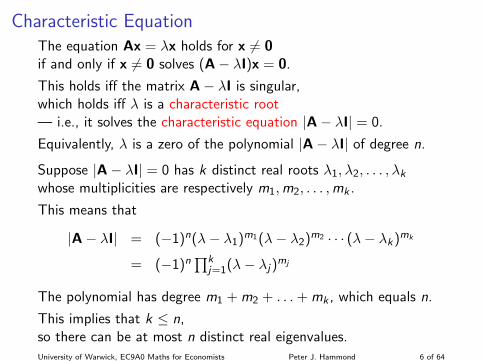
Characteristic EquationThe equation Ax = λx holds for x 6= 0if and only if x 6= 0 solves (A− λI)x = 0.
This holds iff the matrix A− λI is singular,which holds iff λ is a characteristic root— i.e., it solves the characteristic equation |A− λI| = 0.
Equivalently, λ is a zero of the polynomial |A− λI| of degree n.
Suppose |A− λI| = 0 has k distinct real roots λ1, λ2, . . . , λkwhose multiplicities are respectively m1,m2, . . . ,mk .
This means that
|A− λI| = (−1)n(λ− λ1)m1(λ− λ2)m2 · · · (λ− λk)mk
= (−1)n∏k
j=1(λ− λj)mj
The polynomial has degree m1 + m2 + . . .+ mk , which equals n.
This implies that k ≤ n,so there can be at most n distinct real eigenvalues.University of Warwick, EC9A0 Maths for Economists Peter J. Hammond 6 of 64
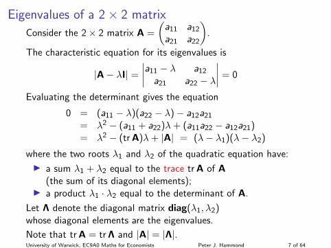
Eigenvalues of a 2× 2 matrix
Consider the 2× 2 matrix A =
(a11 a12a21 a22
).
The characteristic equation for its eigenvalues is
|A− λI| =
∣∣∣∣a11 − λ a12a21 a22 − λ
∣∣∣∣ = 0
Evaluating the determinant gives the equation
0 = (a11 − λ)(a22 − λ)− a12a21= λ2 − (a11 + a22)λ+ (a11a22 − a12a21)= λ2 − (tr A)λ+ |A| = (λ− λ1)(λ− λ2)
where the two roots λ1 and λ2 of the quadratic equation have:
I a sum λ1 + λ2 equal to the trace tr A of A(the sum of its diagonal elements);
I a product λ1 · λ2 equal to the determinant of A.
Let Λ denote the diagonal matrix diag(λ1, λ2)whose diagonal elements are the eigenvalues.
Note that tr A = tr Λ and |A| = |Λ|.University of Warwick, EC9A0 Maths for Economists Peter J. Hammond 7 of 64
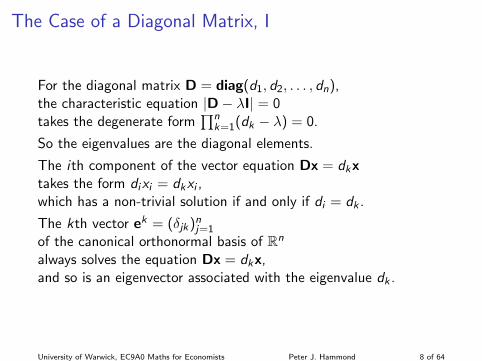
The Case of a Diagonal Matrix, I
For the diagonal matrix D = diag(d1, d2, . . . , dn),the characteristic equation |D− λI| = 0takes the degenerate form
∏nk=1(dk − λ) = 0.
So the eigenvalues are the diagonal elements.
The ith component of the vector equation Dx = dkxtakes the form dixi = dkxi ,which has a non-trivial solution if and only if di = dk .
The kth vector ek = (δjk)nj=1
of the canonical orthonormal basis of Rn
always solves the equation Dx = dkx,and so is an eigenvector associated with the eigenvalue dk .
University of Warwick, EC9A0 Maths for Economists Peter J. Hammond 8 of 64
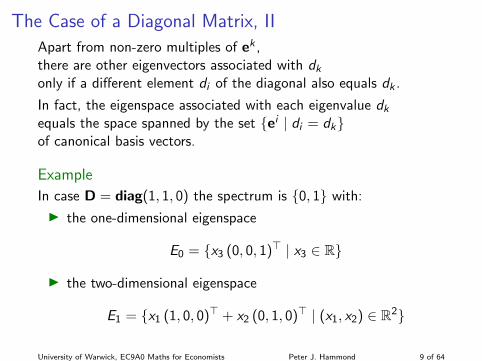
The Case of a Diagonal Matrix, II
Apart from non-zero multiples of ek ,there are other eigenvectors associated with dkonly if a different element di of the diagonal also equals dk .
In fact, the eigenspace associated with each eigenvalue dkequals the space spanned by the set {ei | di = dk}of canonical basis vectors.
Example
In case D = diag(1, 1, 0) the spectrum is {0, 1} with:
I the one-dimensional eigenspace
E0 = {x3 (0, 0, 1)> | x3 ∈ R}
I the two-dimensional eigenspace
E1 = {x1 (1, 0, 0)> + x2 (0, 1, 0)> | (x1, x2) ∈ R2}
University of Warwick, EC9A0 Maths for Economists Peter J. Hammond 9 of 64
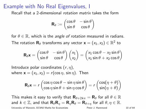
Example with No Real Eigenvalues, IRecall that a 2-dimensional rotation matrix takes the form
Rθ :=
(cos θ − sin θsin θ cos θ
)for θ ∈ R, which is the angle of rotation measured in radians.
The rotation Rθ transforms any vector x = (x1, x2) ∈ R2 to
Rθx =
(cos θ − sin θsin θ cos θ
)(x1x2
)=
(x1 cos θ − x2 sin θx1 sin θ + x2 cos θ
)Introduce polar coordinates (r , η),where x = (x1, x2) = r(cos η, sin η). Then
Rθx = r
(cos η cos θ − sin η sin θcos η sin θ + sin η cos θ
)= r
(cos(η + θ)sin(η + θ)
)This makes it easy to verify that Rθ+2kπ = Rθ for all θ ∈ Rand k ∈ Z, and that RθRη = RηRθ = Rθ+η for all θ, η ∈ R.University of Warwick, EC9A0 Maths for Economists Peter J. Hammond 10 of 64
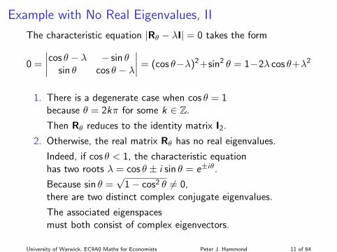
Example with No Real Eigenvalues, II
The characteristic equation |Rθ − λI| = 0 takes the form
0 =
∣∣∣∣cos θ − λ − sin θsin θ cos θ − λ
∣∣∣∣ = (cos θ−λ)2+sin2 θ = 1−2λ cos θ+λ2
1. There is a degenerate case when cos θ = 1because θ = 2kπ for some k ∈ Z.
Then Rθ reduces to the identity matrix I2.
2. Otherwise, the real matrix Rθ has no real eigenvalues.
Indeed, if cos θ < 1, the characteristic equationhas two roots λ = cos θ ± i sin θ = e±iθ.
Because sin θ =√
1− cos2 θ 6= 0,there are two distinct complex conjugate eigenvalues.
The associated eigenspacesmust both consist of complex eigenvectors.
University of Warwick, EC9A0 Maths for Economists Peter J. Hammond 11 of 64
OutlineEigenvalues and Eigenvectors
Real CaseThe Complex CaseLinear Independence of Eigenvectors
Diagonalizing a General MatrixSimilar Matrices
Properties of Adjoint and Symmetric MatricesAn Adjoint Matrix has only Real EigenvaluesThe Spectrum of a Self-Adjoint Matrix
Diagonalizing a Symmetric MatrixOrthogonal MatricesOrthogonal ProjectionsRayleigh QuotientThe Spectral Theorem
Quadratic Forms and Their DefinitenessQuadratic FormsThe Eigenvalue Test of Definiteness
University of Warwick, EC9A0 Maths for Economists Peter J. Hammond 12 of 64
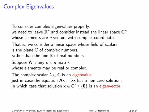
Complex Eigenvalues
To consider complex eigenvalues properly,we need to leave Rn and consider instead the linear space Cn
whose elements are n-vectors with complex coordinates.
That is, we consider a linear space whose field of scalarsis the plane C of complex numbers,rather than the line R of real numbers.
Suppose A is any n × n matrixwhose elements may be real or complex.
The complex scalar λ ∈ C is an eigenvaluejust in case the equation Ax = λx has a non-zero solution,in which case that solution x ∈ Cn \ {0} is an eigenvector.
University of Warwick, EC9A0 Maths for Economists Peter J. Hammond 13 of 64
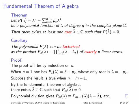
Fundamental Theorem of Algebra
TheoremLet P(λ) = λn +
∑n−1k=0 pkλ
k
be a polynomial function of λ of degree n in the complex plane C.
Then there exists at least one root λ ∈ C such that P(λ) = 0.
Corollary
The polynomial P(λ) can be factorizedas the product Pn(λ) ≡
∏nr=1(λ− λr ) of exactly n linear terms.
Proof.The proof will be by induction on n.
When n = 1 one has P1(λ) = λ+ p0, whose only root is λ = −p0.
Suppose the result is true when n = m − 1.
By the fundamental theorem of algebra,there exists λ ∈ C such that Pm(λ) = 0.
Polynomial division gives Pm(λ) ≡ Pm−1(λ)(λ− λ), etc.
University of Warwick, EC9A0 Maths for Economists Peter J. Hammond 14 of 64
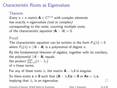
Characteristic Roots as Eigenvalues
TheoremEvery n × n matrix A ∈ Cn×n with complex elementshas exactly n eigenvalues (real or complex)corresponding to the roots, counting multiple roots,of the characteristic equation |A− λI| = 0.
Proof.The characteristic equation can be written in the form Pn(λ) = 0where Pn(λ) ≡ |λI− A| is a polynomial of degree n.
By the fundamental theorem of algebra, together with its corollary,the polynomial |λI− A| equalsthe product
∏nr=1(λ− λr )
of n linear terms.
For any of these roots λr the matrix A− λr I is singular.
So there exists x 6= 0 such that (A− λr I)x = 0 or Ax = λrx,implying that λr is an eigenvalue.
University of Warwick, EC9A0 Maths for Economists Peter J. Hammond 15 of 64
OutlineEigenvalues and Eigenvectors
Real CaseThe Complex CaseLinear Independence of Eigenvectors
Diagonalizing a General MatrixSimilar Matrices
Properties of Adjoint and Symmetric MatricesAn Adjoint Matrix has only Real EigenvaluesThe Spectrum of a Self-Adjoint Matrix
Diagonalizing a Symmetric MatrixOrthogonal MatricesOrthogonal ProjectionsRayleigh QuotientThe Spectral Theorem
Quadratic Forms and Their DefinitenessQuadratic FormsThe Eigenvalue Test of Definiteness
University of Warwick, EC9A0 Maths for Economists Peter J. Hammond 16 of 64
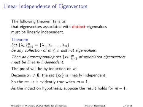
Linear Independence of Eigenvectors
The following theorem tells usthat eigenvectors associated with distinct eigenvaluesmust be linearly independent.
TheoremLet {λk}mk=1 = {λ1, λ2, . . . , λm}be any collection of m ≤ n distinct eigenvalues.
Then any corresponding set {xk}mk=1 of associated eigenvectorsmust be linearly independent.
The proof will be by induction on m.
Because x1 6= 0, the set {x1} is linearly independent.
So the result is evidently true when m = 1.
As the induction hypothesis, suppose the result holds for m − 1.
University of Warwick, EC9A0 Maths for Economists Peter J. Hammond 17 of 64
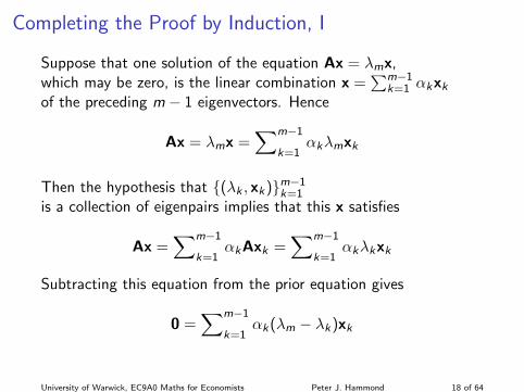
Completing the Proof by Induction, I
Suppose that one solution of the equation Ax = λmx,which may be zero, is the linear combination x =
∑m−1k=1 αkxk
of the preceding m − 1 eigenvectors. Hence
Ax = λmx =∑m−1
k=1αkλmxk
Then the hypothesis that {(λk , xk)}m−1k=1is a collection of eigenpairs implies that this x satisfies
Ax =∑m−1
k=1αkAxk =
∑m−1
k=1αkλkxk
Subtracting this equation from the prior equation gives
0 =∑m−1
k=1αk(λm − λk)xk
University of Warwick, EC9A0 Maths for Economists Peter J. Hammond 18 of 64
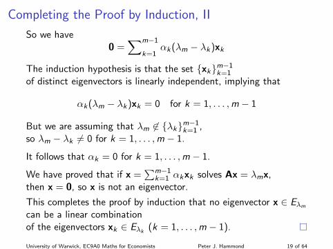
Completing the Proof by Induction, II
So we have0 =
∑m−1
k=1αk(λm − λk)xk
The induction hypothesis is that the set {xk}m−1k=1of distinct eigenvectors is linearly independent, implying that
αk(λm − λk)xk = 0 for k = 1, . . . ,m − 1
But we are assuming that λm 6∈ {λk}m−1k=1 ,so λm − λk 6= 0 for k = 1, . . . ,m − 1.
It follows that αk = 0 for k = 1, . . . ,m − 1.
We have proved that if x =∑m−1
k=1 αkxk solves Ax = λmx,then x = 0, so x is not an eigenvector.
This completes the proof by induction that no eigenvector x ∈ Eλm
can be a linear combinationof the eigenvectors xk ∈ Eλk
(k = 1, . . . ,m − 1).
University of Warwick, EC9A0 Maths for Economists Peter J. Hammond 19 of 64
OutlineEigenvalues and Eigenvectors
Real CaseThe Complex CaseLinear Independence of Eigenvectors
Diagonalizing a General MatrixSimilar Matrices
Properties of Adjoint and Symmetric MatricesAn Adjoint Matrix has only Real EigenvaluesThe Spectrum of a Self-Adjoint Matrix
Diagonalizing a Symmetric MatrixOrthogonal MatricesOrthogonal ProjectionsRayleigh QuotientThe Spectral Theorem
Quadratic Forms and Their DefinitenessQuadratic FormsThe Eigenvalue Test of Definiteness
University of Warwick, EC9A0 Maths for Economists Peter J. Hammond 20 of 64
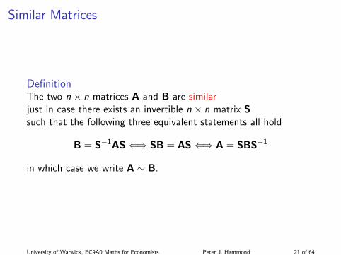
Similar Matrices
DefinitionThe two n × n matrices A and B are similarjust in case there exists an invertible n × n matrix Ssuch that the following three equivalent statements all hold
B = S−1AS⇐⇒ SB = AS⇐⇒ A = SBS−1
in which case we write A ∼ B.
University of Warwick, EC9A0 Maths for Economists Peter J. Hammond 21 of 64
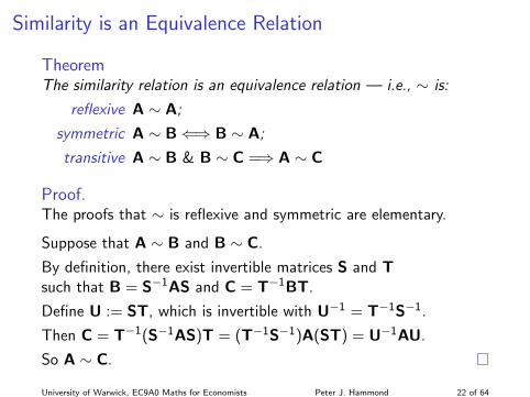
Similarity is an Equivalence Relation
TheoremThe similarity relation is an equivalence relation — i.e., ∼ is:
reflexive A ∼ A;
symmetric A ∼ B⇐⇒ B ∼ A;
transitive A ∼ B & B ∼ C =⇒ A ∼ C
Proof.The proofs that ∼ is reflexive and symmetric are elementary.
Suppose that A ∼ B and B ∼ C.
By definition, there exist invertible matrices S and Tsuch that B = S−1AS and C = T−1BT.
Define U := ST, which is invertible with U−1 = T−1S−1.
Then C = T−1(S−1AS)T = (T−1S−1)A(ST) = U−1AU.
So A ∼ C.
University of Warwick, EC9A0 Maths for Economists Peter J. Hammond 22 of 64
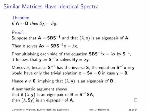
Similar Matrices Have Identical Spectra
TheoremIf A ∼ B then SA = SB.
Proof.Suppose that A = SBS−1 and that (λ, x) is an eigenpair of A.
Then x solves Ax = SBS−1x = λx.
Premultiplying each side of the equation SBS−1x = λx by S−1,it follows that y := S−1x solves By = λy.
Moreover, because S−1 has the inverse S, the equation S−1x = ywould have only the trivial solution x = Sy = 0 in case y = 0.
Hence y 6= 0, implying that (λ, y) is an eigenpair of B.
A symmetric argument showsthat if (λ, y) is an eigenpair of B = S−1SA,then (λ,Sy) is an eigenpair of A.
University of Warwick, EC9A0 Maths for Economists Peter J. Hammond 23 of 64
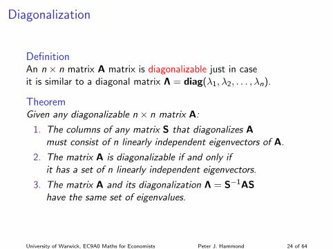
Diagonalization
DefinitionAn n × n matrix A matrix is diagonalizable just in caseit is similar to a diagonal matrix Λ = diag(λ1, λ2, . . . , λn).
TheoremGiven any diagonalizable n × n matrix A:
1. The columns of any matrix S that diagonalizes Amust consist of n linearly independent eigenvectors of A.
2. The matrix A is diagonalizable if and only ifit has a set of n linearly independent eigenvectors.
3. The matrix A and its diagonalization Λ = S−1AShave the same set of eigenvalues.
University of Warwick, EC9A0 Maths for Economists Peter J. Hammond 24 of 64
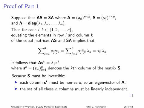
Proof of Part 1
Suppose that AS = SΛ where A = (aij)n×n, S = (sij)
n×n,and Λ = diag(λ1, λ2, . . . , λn).
Then for each i , k ∈ {1, 2, . . . , n},equating the elements in row i and column kof the equal matrices AS and SΛ implies that∑n
j=1aijsjk =
∑n
j=1sijδjkλk = sikλk
It follows that Ask = λksk
where sk = (sik)ni=1 denotes the kth column of the matrix S.
Because S must be invertible:
I each column sk must be non-zero, so an eigenvector of A;
I the set of all these n columns must be linearly independent.
University of Warwick, EC9A0 Maths for Economists Peter J. Hammond 25 of 64
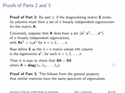
Proofs of Parts 2 and 3
Proof of Part 2: By part 1, if the diagonalizing matrix S exists,its columns must form a set of n linearly independent eigenvectorsfor the matrix A.
Conversely, suppose that A does have a set {x1, x2, . . . , xn}of n linearly independent eigenvectors,with Axk = λkxk for k = 1, 2, . . . , n.
Now define S as the n × n matrix whose kth columnis the eigenvector xk , for each k = 1, 2, . . . , n.
Then it is easy to check that AS = SΛwhere Λ = diag(λ1, λ2, . . . , λn).
Proof of Part 3: This follows from the general propertythat similar matrices have the same spectrum of eigenvalues.
University of Warwick, EC9A0 Maths for Economists Peter J. Hammond 26 of 64
OutlineEigenvalues and Eigenvectors
Real CaseThe Complex CaseLinear Independence of Eigenvectors
Diagonalizing a General MatrixSimilar Matrices
Properties of Adjoint and Symmetric MatricesAn Adjoint Matrix has only Real EigenvaluesThe Spectrum of a Self-Adjoint Matrix
Diagonalizing a Symmetric MatrixOrthogonal MatricesOrthogonal ProjectionsRayleigh QuotientThe Spectral Theorem
Quadratic Forms and Their DefinitenessQuadratic FormsThe Eigenvalue Test of Definiteness
University of Warwick, EC9A0 Maths for Economists Peter J. Hammond 27 of 64
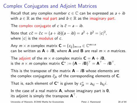
Complex Conjugates and Adjoint MatricesRecall that any complex number c ∈ C can be expressed as a + ibwith a ∈ R as the real part and b ∈ R as the imaginary part.
The complex conjugate of c is c = a− ib.
Note that cc = cc = (a + ib)(a− ib) = a2 + b2 = |c|2,where |c | is the modulus of c.
Any m × n complex matrix C = (cij)m×n ∈ Cm×n
can be written as A + iB, where A and B are real m × n matrices.
The adjoint of the m × n complex matrix C = A + iB,is the n ×m complex matrix C∗ := (A− iB)> = A> − iB>.
This is the transpose of the matrix A− iB whose elements arethe complex conjugates cjk of the corresponding elements of C.
That is, each element of C∗ is given by c∗jk = akj − bkj i .
In the case of a real matrix A, whose imaginary part is 0,its adjoint is simply the transpose A>.
University of Warwick, EC9A0 Maths for Economists Peter J. Hammond 28 of 64
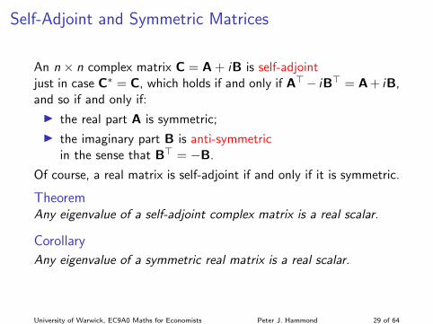
Self-Adjoint and Symmetric Matrices
An n × n complex matrix C = A + iB is self-adjointjust in case C∗ = C, which holds if and only if A>− iB> = A + iB,and so if and only if:
I the real part A is symmetric;
I the imaginary part B is anti-symmetricin the sense that B> = −B.
Of course, a real matrix is self-adjoint if and only if it is symmetric.
TheoremAny eigenvalue of a self-adjoint complex matrix is a real scalar.
Corollary
Any eigenvalue of a symmetric real matrix is a real scalar.
University of Warwick, EC9A0 Maths for Economists Peter J. Hammond 29 of 64
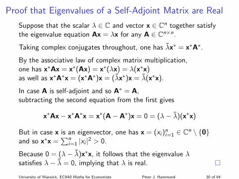
Proof that Eigenvalues of a Self-Adjoint Matrix are Real
Suppose that the scalar λ ∈ C and vector x ∈ Cn together satisfythe eigenvalue equation Ax = λx for any A ∈ Cn×n.
Taking complex conjugates throughout, one has λx∗ = x∗A∗.
By the associative law of complex matrix multiplication,one has x∗Ax = x∗(Ax) = x∗(λx) = λ(x∗x)as well as x∗A∗x = (x∗A∗)x = (λx∗)x = λ(x∗x).
In case A is self-adjoint and so A∗ = A,subtracting the second equation from the first gives
x∗Ax− x∗A∗x = x∗(A− A∗)x = 0 = (λ− λ)(x∗x)
But in case x is an eigenvector, one has x = (xi )ni=1 ∈ Cn \ {0}
and so x∗x =∑n
i=1 |xi |2 > 0.
Because 0 = (λ− λ)x∗x, it follows that the eigenvalue λsatisfies λ− λ = 0, implying that λ is real.
University of Warwick, EC9A0 Maths for Economists Peter J. Hammond 30 of 64
OutlineEigenvalues and Eigenvectors
Real CaseThe Complex CaseLinear Independence of Eigenvectors
Diagonalizing a General MatrixSimilar Matrices
Properties of Adjoint and Symmetric MatricesAn Adjoint Matrix has only Real EigenvaluesThe Spectrum of a Self-Adjoint Matrix
Diagonalizing a Symmetric MatrixOrthogonal MatricesOrthogonal ProjectionsRayleigh QuotientThe Spectral Theorem
Quadratic Forms and Their DefinitenessQuadratic FormsThe Eigenvalue Test of Definiteness
University of Warwick, EC9A0 Maths for Economists Peter J. Hammond 31 of 64

Art Transcends Physics?
University of Warwick, EC9A0 Maths for Economists Peter J. Hammond 32 of 64
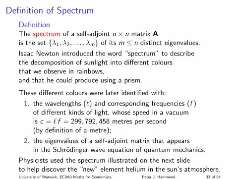
Definition of Spectrum
DefinitionThe spectrum of a self-adjoint n × n matrix Ais the set {λ1, λ2, . . . , λm} of its m ≤ n distinct eigenvalues.
Isaac Newton introduced the word “spectrum” to describethe decomposition of sunlight into different coloursthat we observe in rainbows,and that he could produce using a prism.
These different colours were later identified with:
1. the wavelengths (`) and corresponding frequencies (f )of different kinds of light, whose speed in a vacuumis c = ` f = 299, 792, 458 metres per second(by definition of a metre);
2. the eigenvalues of a self-adjoint matrix that appearsin the Schrodinger wave equation of quantum mechanics.
Physicists used the spectrum illustrated on the next slideto help discover the “new” element helium in the sun’s atmosphere.University of Warwick, EC9A0 Maths for Economists Peter J. Hammond 33 of 64
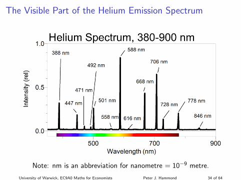
The Visible Part of the Helium Emission Spectrum
Note: nm is an abbreviation for nanometre = 10−9 metre.
University of Warwick, EC9A0 Maths for Economists Peter J. Hammond 34 of 64
OutlineEigenvalues and Eigenvectors
Real CaseThe Complex CaseLinear Independence of Eigenvectors
Diagonalizing a General MatrixSimilar Matrices
Properties of Adjoint and Symmetric MatricesAn Adjoint Matrix has only Real EigenvaluesThe Spectrum of a Self-Adjoint Matrix
Diagonalizing a Symmetric MatrixOrthogonal MatricesOrthogonal ProjectionsRayleigh QuotientThe Spectral Theorem
Quadratic Forms and Their DefinitenessQuadratic FormsThe Eigenvalue Test of Definiteness
University of Warwick, EC9A0 Maths for Economists Peter J. Hammond 35 of 64
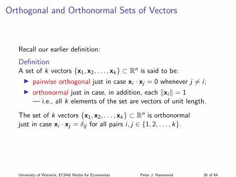
Orthogonal and Orthonormal Sets of Vectors
Recall our earlier definition:
DefinitionA set of k vectors {x1, x2, . . . , xk} ⊂ Rn is said to be:
I pairwise orthogonal just in case xi · xj = 0 whenever j 6= i ;
I orthonormal just in case, in addition, each ‖xi‖ = 1— i.e., all k elements of the set are vectors of unit length.
The set of k vectors {x1, x2, . . . , xk} ⊂ Rn is orthonormaljust in case xi · xj = δij for all pairs i , j ∈ {1, 2, . . . , k}.
University of Warwick, EC9A0 Maths for Economists Peter J. Hammond 36 of 64
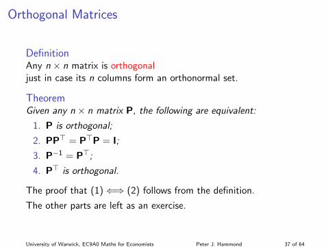
Orthogonal Matrices
DefinitionAny n × n matrix is orthogonaljust in case its n columns form an orthonormal set.
TheoremGiven any n × n matrix P, the following are equivalent:
1. P is orthogonal;
2. PP> = P>P = I;
3. P−1 = P>;
4. P> is orthogonal.
The proof that (1)⇐⇒ (2) follows from the definition.
The other parts are left as an exercise.
University of Warwick, EC9A0 Maths for Economists Peter J. Hammond 37 of 64
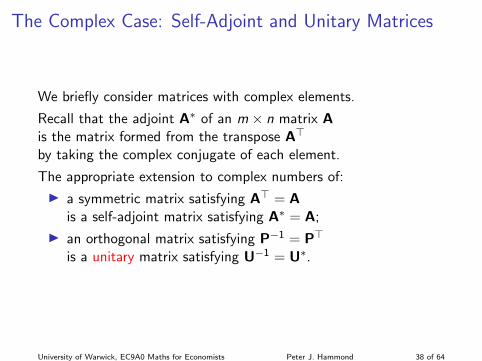
The Complex Case: Self-Adjoint and Unitary Matrices
We briefly consider matrices with complex elements.
Recall that the adjoint A∗ of an m × n matrix Ais the matrix formed from the transpose A>
by taking the complex conjugate of each element.
The appropriate extension to complex numbers of:
I a symmetric matrix satisfying A> = Ais a self-adjoint matrix satisfying A∗ = A;
I an orthogonal matrix satisfying P−1 = P>
is a unitary matrix satisfying U−1 = U∗.
University of Warwick, EC9A0 Maths for Economists Peter J. Hammond 38 of 64
OutlineEigenvalues and Eigenvectors
Real CaseThe Complex CaseLinear Independence of Eigenvectors
Diagonalizing a General MatrixSimilar Matrices
Properties of Adjoint and Symmetric MatricesAn Adjoint Matrix has only Real EigenvaluesThe Spectrum of a Self-Adjoint Matrix
Diagonalizing a Symmetric MatrixOrthogonal MatricesOrthogonal ProjectionsRayleigh QuotientThe Spectral Theorem
Quadratic Forms and Their DefinitenessQuadratic FormsThe Eigenvalue Test of Definiteness
University of Warwick, EC9A0 Maths for Economists Peter J. Hammond 39 of 64
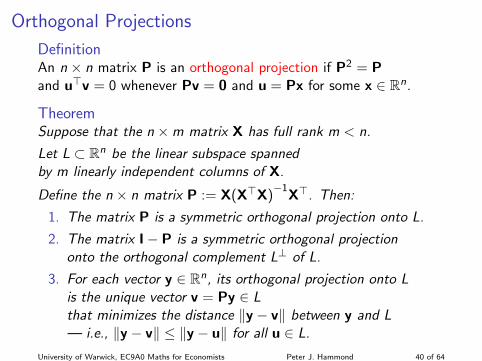
Orthogonal Projections
DefinitionAn n × n matrix P is an orthogonal projection if P2 = Pand u>v = 0 whenever Pv = 0 and u = Px for some x ∈ Rn.
TheoremSuppose that the n ×m matrix X has full rank m < n.
Let L ⊂ Rn be the linear subspace spannedby m linearly independent columns of X.
Define the n × n matrix P := X(X>X)−1
X>. Then:
1. The matrix P is a symmetric orthogonal projection onto L.
2. The matrix I− P is a symmetric orthogonal projectiononto the orthogonal complement L⊥ of L.
3. For each vector y ∈ Rn, its orthogonal projection onto Lis the unique vector v = Py ∈ Lthat minimizes the distance ‖y − v‖ between y and L— i.e., ‖y − v‖ ≤ ‖y − u‖ for all u ∈ L.
University of Warwick, EC9A0 Maths for Economists Peter J. Hammond 40 of 64
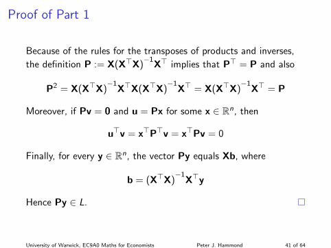
Proof of Part 1
Because of the rules for the transposes of products and inverses,
the definition P := X(X>X)−1
X> implies that P> = P and also
P2 = X(X>X)−1
X>X(X>X)−1
X> = X(X>X)−1
X> = P
Moreover, if Pv = 0 and u = Px for some x ∈ Rn, then
u>v = x>P>v = x>Pv = 0
Finally, for every y ∈ Rn, the vector Py equals Xb, where
b = (X>X)−1
X>y
Hence Py ∈ L.
University of Warwick, EC9A0 Maths for Economists Peter J. Hammond 41 of 64
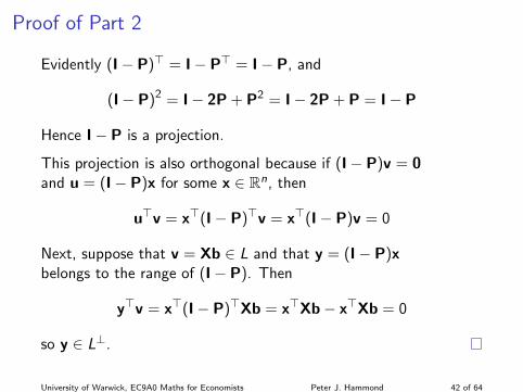
Proof of Part 2
Evidently (I− P)> = I− P> = I− P, and
(I− P)2 = I− 2P + P2 = I− 2P + P = I− P
Hence I− P is a projection.
This projection is also orthogonal because if (I− P)v = 0and u = (I− P)x for some x ∈ Rn, then
u>v = x>(I− P)>v = x>(I− P)v = 0
Next, suppose that v = Xb ∈ L and that y = (I− P)xbelongs to the range of (I− P). Then
y>v = x>(I− P)>Xb = x>Xb− x>Xb = 0
so y ∈ L⊥.
University of Warwick, EC9A0 Maths for Economists Peter J. Hammond 42 of 64
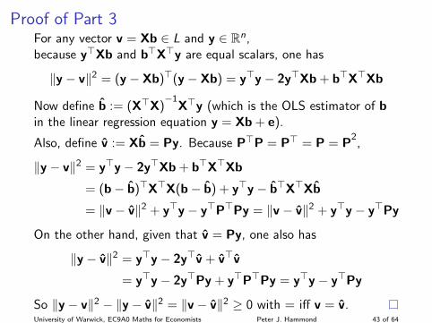
Proof of Part 3For any vector v = Xb ∈ L and y ∈ Rn,because y>Xb and b>X>y are equal scalars, one has
‖y − v‖2 = (y − Xb)>(y − Xb) = y>y − 2y>Xb + b>X>Xb
Now define b := (X>X)−1
X>y (which is the OLS estimator of bin the linear regression equation y = Xb + e).
Also, define v := Xb = Py. Because P>P = P> = P = P2,
‖y − v‖2 = y>y − 2y>Xb + b>X>Xb
= (b− b)>X>X(b− b) + y>y − b>X>Xb
= ‖v − v‖2 + y>y − y>P>Py = ‖v − v‖2 + y>y − y>Py
On the other hand, given that v = Py, one also has
‖y − v‖2 = y>y − 2y>v + v>v
= y>y − 2y>Py + y>P>Py = y>y − y>Py
So ‖y − v‖2 − ‖y − v‖2 = ‖v − v‖2 ≥ 0 with = iff v = v.University of Warwick, EC9A0 Maths for Economists Peter J. Hammond 43 of 64
OutlineEigenvalues and Eigenvectors
Real CaseThe Complex CaseLinear Independence of Eigenvectors
Diagonalizing a General MatrixSimilar Matrices
Properties of Adjoint and Symmetric MatricesAn Adjoint Matrix has only Real EigenvaluesThe Spectrum of a Self-Adjoint Matrix
Diagonalizing a Symmetric MatrixOrthogonal MatricesOrthogonal ProjectionsRayleigh QuotientThe Spectral Theorem
Quadratic Forms and Their DefinitenessQuadratic FormsThe Eigenvalue Test of Definiteness
University of Warwick, EC9A0 Maths for Economists Peter J. Hammond 44 of 64
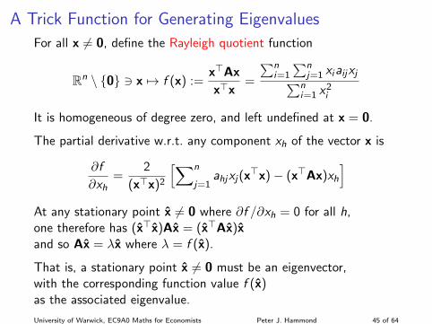
A Trick Function for Generating Eigenvalues
For all x 6= 0, define the Rayleigh quotient function
Rn \ {0} 3 x 7→ f (x) :=x>Ax
x>x=
∑ni=1
∑nj=1 xiaijxj∑n
i=1 x2i
It is homogeneous of degree zero, and left undefined at x = 0.
The partial derivative w.r.t. any component xh of the vector x is
∂f
∂xh=
2
(x>x)2
[∑n
j=1ahjxj(x>x)− (x>Ax)xh
]At any stationary point x 6= 0 where ∂f /∂xh = 0 for all h,one therefore has (x>x)Ax = (x>Ax)xand so Ax = λx where λ = f (x).
That is, a stationary point x 6= 0 must be an eigenvector,with the corresponding function value f (x)as the associated eigenvalue.
University of Warwick, EC9A0 Maths for Economists Peter J. Hammond 45 of 64
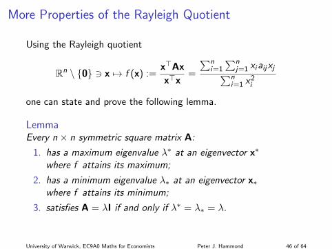
More Properties of the Rayleigh Quotient
Using the Rayleigh quotient
Rn \ {0} 3 x 7→ f (x) :=x>Ax
x>x=
∑ni=1
∑nj=1 xiaijxj∑n
i=1 x2i
one can state and prove the following lemma.
LemmaEvery n × n symmetric square matrix A:
1. has a maximum eigenvalue λ∗ at an eigenvector x∗
where f attains its maximum;
2. has a minimum eigenvalue λ∗ at an eigenvector x∗where f attains its minimum;
3. satisfies A = λI if and only if λ∗ = λ∗ = λ.
University of Warwick, EC9A0 Maths for Economists Peter J. Hammond 46 of 64
Proof of Parts 1 and 2
The unit sphere Sn−1 is a compact subset of Rn,and the Rayleigh quotient function f restricted to Sn−1
is continuous.
By the extreme value theorem, f restricted to Sn−1 must have:
I a maximum value λ∗ attained at some point x∗;
I a minimum value λ∗ attained at some point x∗.
Because f is homogeneous of degree zero,these are the maximum and minimum values of fover the whole domain Rn \ {0}.
In particular, f must be stationary at any maximum point x∗,as well as at any minimum point x∗.
But stationary points must be eigenvectors.
This proves parts 1 and 2 of the lemma.
University of Warwick, EC9A0 Maths for Economists Peter J. Hammond 47 of 64
OutlineEigenvalues and Eigenvectors
Real CaseThe Complex CaseLinear Independence of Eigenvectors
Diagonalizing a General MatrixSimilar Matrices
Properties of Adjoint and Symmetric MatricesAn Adjoint Matrix has only Real EigenvaluesThe Spectrum of a Self-Adjoint Matrix
Diagonalizing a Symmetric MatrixOrthogonal MatricesOrthogonal ProjectionsRayleigh QuotientThe Spectral Theorem
Quadratic Forms and Their DefinitenessQuadratic FormsThe Eigenvalue Test of Definiteness
University of Warwick, EC9A0 Maths for Economists Peter J. Hammond 48 of 64
A Useful Lemma
LemmaLet A be a symmetric n × n matrix.
Suppose that there are m < n eigenvectors {uk}mk=1
which form an orthonormal set of vectors,as well as the columns of an n ×m matrix U.
Then there is at least one more eigenvector xthat satisfies U>x = 0— i.e., it is orthogonal to each of the m eigenvectors uk .
University of Warwick, EC9A0 Maths for Economists Peter J. Hammond 49 of 64
Constructive Proof, Part 1
For each eigenvector uk , let λk be the associated eigenvalue,so that Auk = λkuk for k = 1, 2, . . . ,m.
Then AU = UΛ where Λ := diag(λk)nk=1.
Also, because the eigenvectors {uk}mk=1 form an orthonormal set,one has U>U = Im.
Hence U>AU = U>UΛ = Λ.
Also, transposing AU = UΛ gives U>A = ΛU>.
University of Warwick, EC9A0 Maths for Economists Peter J. Hammond 50 of 64
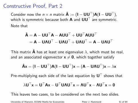
Constructive Proof, Part 2
Consider now the n × n matrix A := (I−UU>)A(I−UU>),which is symmetric because both A and UU> are symmetric.
Note that
A = A−UU>A− AUU> + UU>AUU>
= A−UΛU> −UΛU> + UΛU> = A−UΛU>
This matrix A has at least one eigenvalue λ, which must be real,and an associated eigenvector x 6= 0, which together satisfy
Ax = (I−UU>)A(I−UU>)x = (A−UΛU>)x = λx
Pre-multiplying each side of the last equation by U> shows that
λU>x = U>Ax−U>UΛU>x = ΛU>x− ΛU>x = 0
This leaves two cases, to be considered on the next two slides.
University of Warwick, EC9A0 Maths for Economists Peter J. Hammond 51 of 64
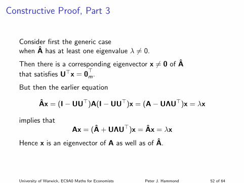
Constructive Proof, Part 3
Consider first the generic casewhen A has at least one eigenvalue λ 6= 0.
Then there is a corresponding eigenvector x 6= 0 of A
that satisfies U>x = 0>m.
But then the earlier equation
Ax = (I−UU>)A(I−UU>)x = (A−UΛU>)x = λx
implies thatAx = (A + UΛU>)x = Ax = λx
Hence x is an eigenvector of A as well as of A.
University of Warwick, EC9A0 Maths for Economists Peter J. Hammond 52 of 64
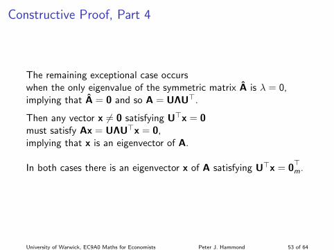
Constructive Proof, Part 4
The remaining exceptional case occurswhen the only eigenvalue of the symmetric matrix A is λ = 0,implying that A = 0 and so A = UΛU>.
Then any vector x 6= 0 satisfying U>x = 0must satisfy Ax = UΛU>x = 0,implying that x is an eigenvector of A.
In both cases there is an eigenvector x of A satisfying U>x = 0>m.
University of Warwick, EC9A0 Maths for Economists Peter J. Hammond 53 of 64
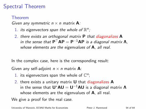
Spectral Theorem
TheoremGiven any symmetric n × n matrix A:
1. its eigenvectors span the whole of Rn;
2. there exists an orthogonal matrix P that diagonalizes Ain the sense that P>AP = P−1AP is a diagonal matrix Λ,whose elements are the eigenvalues of A, all real.
In the complex case, here is the corresponding result:
Given any self-adjoint n × n matrix A:
1. its eigenvectors span the whole of Cn;
2. there exists a unitary matrix U that diagonalizes Ain the sense that U∗AU = U−1AU is a diagonal matrix Λwhose elements are the eigenvalues of A, all real.
We give a proof for the real case.
University of Warwick, EC9A0 Maths for Economists Peter J. Hammond 54 of 64
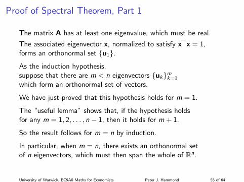
Proof of Spectral Theorem, Part 1
The matrix A has at least one eigenvalue, which must be real.
The associated eigenvector x, normalized to satisfy x>x = 1,forms an orthonormal set {u1}.
As the induction hypothesis,suppose that there are m < n eigenvectors {uk}mk=1
which form an orthonormal set of vectors.
We have just proved that this hypothesis holds for m = 1.
The “useful lemma” shows that, if the hypothesis holdsfor any m = 1, 2, . . . , n − 1, then it holds for m + 1.
So the result follows for m = n by induction.
In particular, when m = n, there exists an orthonormal setof n eigenvectors, which must then span the whole of Rn.
University of Warwick, EC9A0 Maths for Economists Peter J. Hammond 55 of 64
Proof of Spectral Theorem, Part 2
Also, by the previous result, taking P as an orthogonal matrixwhose columns are an orthonormal set of n eigenvectors,we obtain P>AP = P−1AP = Λ.
University of Warwick, EC9A0 Maths for Economists Peter J. Hammond 56 of 64
OutlineEigenvalues and Eigenvectors
Real CaseThe Complex CaseLinear Independence of Eigenvectors
Diagonalizing a General MatrixSimilar Matrices
Properties of Adjoint and Symmetric MatricesAn Adjoint Matrix has only Real EigenvaluesThe Spectrum of a Self-Adjoint Matrix
Diagonalizing a Symmetric MatrixOrthogonal MatricesOrthogonal ProjectionsRayleigh QuotientThe Spectral Theorem
Quadratic Forms and Their DefinitenessQuadratic FormsThe Eigenvalue Test of Definiteness
University of Warwick, EC9A0 Maths for Economists Peter J. Hammond 57 of 64
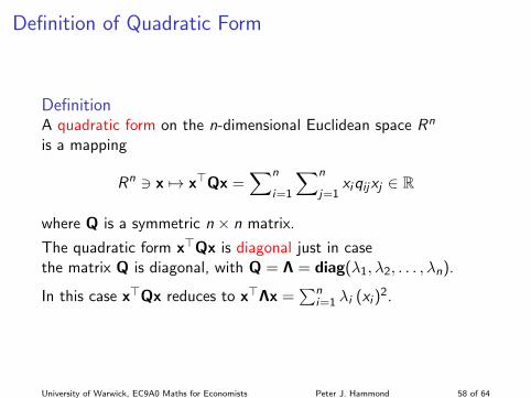
Definition of Quadratic Form
DefinitionA quadratic form on the n-dimensional Euclidean space Rn
is a mapping
Rn 3 x 7→ x>Qx =∑n
i=1
∑n
j=1xiqijxj ∈ R
where Q is a symmetric n × n matrix.
The quadratic form x>Qx is diagonal just in casethe matrix Q is diagonal, with Q = Λ = diag(λ1, λ2, . . . , λn).
In this case x>Qx reduces to x>Λx =∑n
i=1 λi (xi )2.
University of Warwick, EC9A0 Maths for Economists Peter J. Hammond 58 of 64
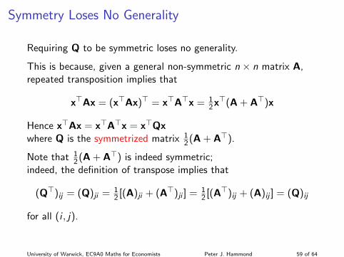
Symmetry Loses No Generality
Requiring Q to be symmetric loses no generality.
This is because, given a general non-symmetric n × n matrix A,repeated transposition implies that
x>Ax = (x>Ax)> = x>A>x = 12x>(A + A>)x
Hence x>Ax = x>A>x = x>Qxwhere Q is the symmetrized matrix 1
2(A + A>).
Note that 12(A + A>) is indeed symmetric;
indeed, the definition of transpose implies that
(Q>)ij = (Q)ji = 12 [(A)ji + (A>)ji ] = 1
2 [(A>)ij + (A)ij ] = (Q)ij
for all (i , j).
University of Warwick, EC9A0 Maths for Economists Peter J. Hammond 59 of 64
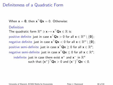
Definiteness of a Quadratic Form
When x = 0, then x>Qx = 0. Otherwise:
DefinitionThe quadratic form Rn 3 x 7→ x>Qx ∈ R is:
positive definite just in case x>Qx > 0 for all x ∈ Rn \ {0};negative definite just in case x>Qx < 0 for all x ∈ Rn \ {0};positive semi-definite just in case x>Qx ≥ 0 for all x ∈ Rn;
negative semi-definite just in case x>Qx ≤ 0 for all x ∈ Rn;
indefinite just in case there exist x+ and x− in Rn
such that (x+)>Qx > 0 and (x−)>Qx < 0.
University of Warwick, EC9A0 Maths for Economists Peter J. Hammond 60 of 64
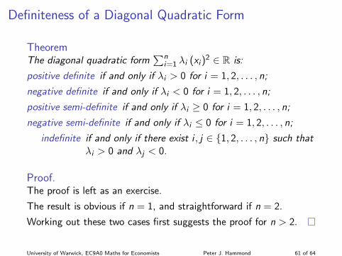
Definiteness of a Diagonal Quadratic Form
TheoremThe diagonal quadratic form
∑ni=1 λi (xi )
2 ∈ R is:
positive definite if and only if λi > 0 for i = 1, 2, . . . , n;
negative definite if and only if λi < 0 for i = 1, 2, . . . , n;
positive semi-definite if and only if λi ≥ 0 for i = 1, 2, . . . , n;
negative semi-definite if and only if λi ≤ 0 for i = 1, 2, . . . , n;
indefinite if and only if there exist i , j ∈ {1, 2, . . . , n} such thatλi > 0 and λj < 0.
Proof.The proof is left as an exercise.
The result is obvious if n = 1, and straightforward if n = 2.
Working out these two cases first suggests the proof for n > 2.
University of Warwick, EC9A0 Maths for Economists Peter J. Hammond 61 of 64
OutlineEigenvalues and Eigenvectors
Real CaseThe Complex CaseLinear Independence of Eigenvectors
Diagonalizing a General MatrixSimilar Matrices
Properties of Adjoint and Symmetric MatricesAn Adjoint Matrix has only Real EigenvaluesThe Spectrum of a Self-Adjoint Matrix
Diagonalizing a Symmetric MatrixOrthogonal MatricesOrthogonal ProjectionsRayleigh QuotientThe Spectral Theorem
Quadratic Forms and Their DefinitenessQuadratic FormsThe Eigenvalue Test of Definiteness
University of Warwick, EC9A0 Maths for Economists Peter J. Hammond 62 of 64
Diagonalizing Quadratic Forms
Consider a quadratic form Rn 3 x 7→ x>Qx ∈ R where,without losing generality,we assume that the n × n matrix Q is symmetric.
By the spectral theorem for symmetric matrices,there exists a matrix P that diagonalizes Q,meaning that P−1QP is a diagonal matrix that we denote by Λ.
Moreover P can be made orthogonal, meaning that P−1 = P>.
Given any x 6= 0, because P−1 exists, we can define y = P−1x.
This implies that x = Py, where y 6= 0 because (P−1)−1 = P.
Then x>Qx = y>P>QPy = y>Λy,so the diagonalization leads to a diagonal quadratic form.
University of Warwick, EC9A0 Maths for Economists Peter J. Hammond 63 of 64
The Eigenvalue Test
A standard result says that Qand its diagonalization P−1QP have the same set of eigenvalues.
From the theorem on the definiteness of a diagonal quadratic form,it follows that:
TheoremThe quadratic form x>Qx is:
positive definite if and only if all its eigenvalues are positive;
negative definite if and only if all its eigenvalues are negative;
positive semi-definite if and only ifall its eigenvalues are non-negative;
negative semi-definite if and only ifall its eigenvalues are non-positive;
indefinite if and only ifit has both positive and negative eigenvalues.
University of Warwick, EC9A0 Maths for Economists Peter J. Hammond 64 of 64