Lecture Notes 4: Colligative Properties  The previous lecture was about solutions and whether they would form or not.  Again, we tackled things in very general terms and really only dealt with extremes.  For mixtures in which ΔGsolution > 0, we said things didn’t dissolve (in reality they will dissolve but only a little bit) for ΔGsolution < 0 we said that they would dissolve (but of course there is always a limit).    Now we want to focus on the properties of solutions.  That is, we will now be looking at the typical situations for the substances that did actually dissolve.  If you remember, we developed some insight into what situations these would be.  For the solution to form, we used the criteria that  ΔGsolution < 0.    We broke this down into how the entropy and enthalpy affect the free energy:  

ΔGsolution = ΔHsolution  ‐ TΔSsolution     

Generally, we said that ΔHsolution > 0, and the ΔSsolution > 0  This meant that for ΔGsolution to be negative we needed  

| TΔSsolution |  > | ΔHsolution|  

One way to try to ensure this was to minimize the enthalpy change.  That is, we wanted the enthalpy of the solution to be the same as the enthalpy of separated solute and solvent.  This meant we need there to be little or no change in the intermolecular forces.  Thus we came up with the idea of “like dissolves like”.  When the intermolecular forces for the solute and the solvent are nearly identical, ΔHsolution is small.  Now we will take that to its ultimate limit and treat the solutions that we are making as ideal.  In an ideal solution we assume that ΔHsolution is so small that it is essentially zero.  That is, the IMF in the solution are not just similar but identical.  This means that all the solution properties arise only from a difference in entropy between the pure substances and the mixture.  The enthalpy (and thus the IMF) is not important.  This has a big consequence.  It means that solutions with different solutes (different IMF) will all be treated essentially the same.    This will be the idea of colligative properties of solutions. 

•  By definition, a colligative property is a property of a solution (an ideal solution) which depends on the amount of the solute in the solution but is not related to the nature of the solute (its IMF don’t matter).  •  The nature of the solvent matters as different solvents are different from one another.  But the nature of the solute does not since we are assuming the solutes are all like the particular solvent we are looking at (like dissolve like).  •  What matters is the entropy of the solution compared to the pure solvent.  This is affected by how much of the solute there is.  In particular, how many particles there are.  Thus 1 mole of sugar = 1 mole of Na+ ions = 1 mole of SO42‐ ions….  There are four properties that we will look at.  All are simply related to the concentration of the solutions.  However, for historical reasons the units for the concentration are different for the different phenomena   They are  

The lowering of Vapor Pressure (Raoult’s Law).   The vapor pressure of a solution will be lower than the pure substance 

The basis of understanding distillation.  A key property of how antifreeze works in your car.   

Boiling Point Elevation.   The boiling point of a solution will be higher than the pure substance. 

This is the same as the lowering of the vapor pressure.  We have handy formula for the boiling point.  

Freezing Point Depression.   The freezing point of a solution will be lower than the pure substance. 

This is why you salt the sidewalk to melt ice.  How you use ice and salt to make ice cream.  

Osmosis.   Explains the movement of solvent between solutions of different concentrations separated by a membrane. 

A critical concept for cell biology.  An important means to purify water. 

Why does the boiling point go up? Why does the freezing point go down? 

Why doesn’t the nature of the solute matter?  

IT IS ALL THE ENTROPY!  

Remember we have assumed the solutions are ideal.   Thus the difference is the entropy, not the enthalpy.  What is different?  The solution has a higher entropy than the pure solvent.  Thus if the enthalpy is the same (we have assumed it is with ideal solution), the free energy of the solution will be lower. G = H –TS.  S is larger.  G must be lower.  Lower free energy = more stable.  We have now created a situation in which the solution is more stable than the pure solvent. Let’s look at the melting temperature of the pure compound; this is the temperature at which the solid and the liquid have the same free energy.  But now, at this same temperature and pressure the solution has a lower free energy.  Now the liquid solution is lower in free energy than the pure solid.  What happens?  It melts spontaneously.  If we want to re‐establish equilibrium between the pure solid and the liquid solution, we need to lower the temperature.  How much?  It depends on how much we have increased the entropy of the solution (how much stuff we have put in it).    

Boiling is the same concept, but we are instead comparing pure vapor to the “mixed‐up” solution.  The means we have effectively increased the stable region of the liquid on the phase diagram.  The diagram on the left shows the phase diagram for a pure substance (pink) compared to a solution (blue).  (for some reason this plot notes the freezing point depression at the triple point.  But the same is true for the freezing point at any pressure) 

The colligative properties all depend on the concentration of the solute.  Again, for historical reason the tabulated constants all utilize different measures for concentration.  The lowering of the Vapor Pressure effect follows Raoult’s Law.  This is like Henry’s Law.  The pressure is proportional to the mole fraction (concentration).  Here it is the mole fraction of solvent.  But we can also write the formula for the mole fraction of solute (see later)  

Psolvent = XsolventP*solvent   P* is the vapor pressure of the pure solvent.  P is the partial pressure of the solvent in the mixture.  And X is the mole fraction (concentration).   Boiling Point Elevation/Freezing Point Depression.  Both of these formulas assume a linear dependence of the change in the phase transition temperature on the molality (concentration) of the solution.  

ΔTf =‐mKf           ΔTb =+mKb           m is the molality of the solution  and Kf  and Kb are constants that depend on the solvent.   The effect of osmosis is quantified by an osmotic pressure  

Π =MRT  Where M is the molarity of the solution, Π is the osmotic pressure, R is the ideal gas constant and T is the temperature. 

Quick review on concentrations.  Let’s have a quick review of these three measures of concentration.  Mole Fraction, molality , and molarity. For each example let’s look at the same solution that contains 50g of sugar (sucrose) as the solute in 117 grams (117 mL) of water as the solvent.  Note: this is a very concentrated solution.  Sucrose has a molecular weight of 342 g mol‐1 , so 50 g is 0.146 moles.   Water has a molecular weight of 18 g mol‐1 so 117 g is 6.5 moles The density of this solution would be 1.34 g cm‐3  Mole Fraction Mole fraction is defined as the moles of one compound compared to the total number of moles.  If we want the mole fraction of the solute it would be  

€

χ solute =moles solutemoles total

=0.146sugar

0.146sugar + 6.5water= 0.022 mole fraction sugar

  Molality Molality is the moles of solute divided by the kilograms of solvent note the density of water is 1 g cm‐3 so 1L of water is 1kg of water   

€

m =moles solutekg solvent

=0.146sugar

0.117kg water=1.25molal  

 Molarity Molarity is the moles of solute divided by the volume of the solution in liters.  To find the volume of the solution we need to know its density.    

€

Vsolution = (mass) /(density) = (167g) /(1.35g mL) =125mL = 0.125L   

€

M =moles soluteL solution

=0.146sugar

0.125L=1.17M  

Another interruption to introduce the “van’t Hoff factor”  What matters for all the colligative properties is the number of solute particles (not what they are).  We need to be careful when dealing with ionic compounds in polar solvents (essentially salts in water), as these compounds break apart into ions and make more particles.    For example, let’s compare the concentration of particles in the following solutions.  1M NaCl 1M Na2SO4 1M MgSO4 1M sucrose  They all have 1 mole solute in 1L of solution.  But the number of particles is different.  How many solute “particles” are there in 1 L of each of these solutions?   1L of 1M NaCl   has  1 mole Na+ ion  and 1 mole of Cl‐ ions    that is 2 moles of “stuff” in the solution  1L of 1M Na2SO4 has  2 mole Na+ ion  and 1 mole of SO42‐ ions    that is 3 moles of “stuff” in the solution  1L of 1M MgSO4   has 1 mole Mg2+ ion  and 1 mole of SO42‐ ions    that is 2 moles of “stuff” in the solution  1L of 1M sucrose   has 1 mole sucrose molecules        that is 1 moles of “stuff” in the solution   To take care of this we introduce a scaling factor to relate the number of particles that result per mole of the compound.  This is the van’t Hoff factor (named after Jacobus Henricus van 't Hoff, a Dutch chemist who was the winner of the first Nobel Prize in Chemistry).  It gets the symbol i.  Our previous formulas for boiling point elevation, freezing point depression, and osmotic pressure can all be modified by multiplying the concentration by i. 

Back to the properties of the solutions.  First we’ll deal with the one that appears a bit different.  Vapor pressure reduction.  Raoult’s Law states   

Psolvent = XsolventP*solvent   Thus, as you add solute to the solution, the mole fraction of the solvent goes down and the partial pressure of the solvent goes down.  This is a bit of an oddball of our properties because it is not written in terms of the concentration of the solute.  We can change that by looking at the change in the vapor pressure.  Let’s write the mole fraction of the solvent in term of the mole fraction of the solute.  What isn’t solvent has to be solute.  Thus the mole fraction of the solvent = 1 – mole fraction of the solute   

€

χ solvent = (1− χ solute )  

€

Psolvent = χ solventPsolvent* = (1− χ solute )Psolvent

* = Psolvent* − χ solutePsolvent

*

ΔP = Psolvent* −Psolvent= χ solutePsolvent

*  

 This last term is the decrease in the vapor pressure of the solvent in the mixture compared to the pure solvent.   This is linearly related to the mole fraction of the solute.  How much does the vapor pressure of our example sugar solution decrease at 25°C where the vapor pressure of pure water is 23.8 Torr?     ΔP = XP* = (.022)(23.8 Torr) = 0.524 Torr  Note: we need to remember this is a decrease.  The vapor pressure of the solution will be 23.8 ‐ .524 Torr = 23.3 Torr 

Important Note About Vapor Pressure  For most colligative properties we are looking at a mixture of a non‐volatile solute (something with a vapor pressure of approximately zero) and a liquid.   For example, NaCl in water, or anthracene in toluene, or a protein in water….  However, we can make mixtures of two volatile liquids in which case both of them have a non‐zero vapor pressure.  

For these cases, if we assume ideality, then Raoult’s Law gives us the partial pressure of each component.  The total vapor pressure will be the sum of the pressure for each liquid.  For example, if we make a mixture of octane and hexane, they both contribute to the total vapor pressure.  However it is easy to figure out the total pressure since it is just the sum of the two partial pressures.    The plot on the left that shows the vapor pressure as function of the mole fraction of octane in the solution.  When the mole fraction is 0, the solution is all hexane.  When the mole fraction is one, then the solution is all octane.  In between, the pressure of each is simply the mole fraction times the vapor pressure of the pure compound. 

 EXAMPLE Imagine that at this temperature the pure vapor pressure of octane was 100 Torr and the pure vapor pressure of hexane was 300 Torr.  What is the total vapor pressure of a solution that contains 2 moles of octane and 8 moles of hexane at this temperature?  First let’s look at the mole fractions and the partial pressure of each. There are 2 moles of octane and 10 total moles for the mole fraction of octane, Xoctane = (2)/(10)=0.2 The mole fraction of hexane is simply 1 – Xoctane = 0.8  (or you can see it is 8/10 = 0.8)  Poctane = XoctaneP*octane = (0.2)(100 Torr) = 20 TorrP Phexane =XhexaneP*hexane =(0.8)(300 Torr) = 240 Torr  Ptotal = Poctane + Phexane = 20 + 240 = 260 Torr 

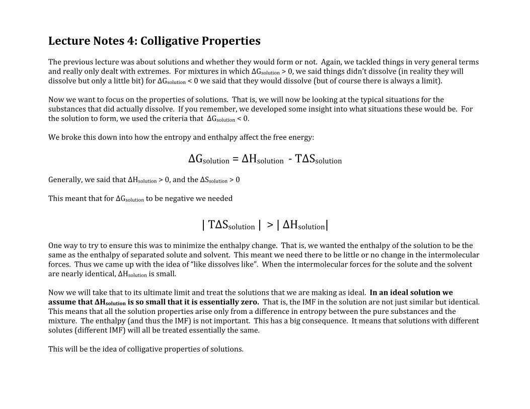
Freezing Point Depression             For water Kf is 1.86 °C molal‐1. So the freezing point change for our sugar solution is  ΔT =‐iKfm= ‐(1)(1.86 °C m‐1)(1.25m)= ‐2.32 °C  The new freezing point is 0°C – 2.32°C = ‐2.32°C 

  Boiling Point Elevation              For water Kb is 0.512 °C molal‐1. So the freezing point change for our sugar solution is  ΔT =iKbm= (1)(0.512 °C m‐1)(1.25m)= 0.64 °C  The new freezing point is 100°C + 0.64°C = 100.64°C 

 Osmotic pressure  

Π =iMRT   Π is the osmotic pressure i is the van’t Hoff factor M is the molarity of the solution R is the ideal gas constant (in the correct units) T is the temperature in Kelvin   What is the osmotic pressure of our sugar solution?  Π = iMRT=(1)(1.17 M)(0.08208 L‐atm K‐1 mol‐1)(298K)=28.6 atm    Note:  If we write molarity as moles/volume    M=n/V  Then our equation becomes  Π=MRT=(n/V)RT    or ΠV=nRT   This is just like the ideal gas law, except we have the osmotic pressure, the volume of the solution, and the number of moles is the moles of solute.  This seems like a surprise, but it has to work out this way because of the units.  

Putting things into perspective.  Let’s compare all four of these effects:   For our highly concentrated sugar solution   ΔT =iKbm= (1)(0.512 °C m‐1)(1.25m)= 0.64 °C ΔT =‐iKfm= ‐(1)(1.86 °C m‐1)(1.25m)= ‐2.32 °C ΔP = XP* = (.022)(23.8 Torr) = 0.524 Torr Π = iMRT=(1)(1.17 M)(0.08208 L‐atm K‐1 mol‐1)(298K)=28.6 atm  The vapor pressure changes by 0.5 Torr (out of 24) or about 2% The boiling point changed by 0.6 °C The freezing point changes by 2.3 °C  But the osmotic pressure is huge!   More than 28 atm!  All of these effects are really quite small.  With the exception of OSMOSIS.  It is important even at low concentrations!  Why do we care if these effects are so small?  Because they can still be important.    Salting the roads can lower the melting temperature by many degrees Celsius to keep the roads from getting icy. Changes in boiling point for mixtures are critical for understanding distillation of mixtures of liquids  Also, these are the changes for ideal solutions.  Non‐ideal solutions can exhibit even bigger effects! 

More on Osmosis  It is really important to understand what osmosis is.  Up to now, I’ve just said there is a thing called osmotic pressure and we can calculate it.  What is osmosis?  What is osmotic pressure?  Osmosis is related to the property of two solutions that are separated by a semi‐permeable membrane.  This membrane has the important property that the solvent can pass through it but the solute can’t.  Yes, one can make such a membrane.  In fact, this is a reasonable first model for cell membranes.   Here is a picture that shows this idea.  On the left hand side of the membrane is a pure solvent.  On the right 

is a solution.  Initially, the free energy will be lower in the solution compared to the pure solvent.  This is what we have been talking about for all the colligative properties.  Given that the free energy in the solution is lower, the solvent will move to the side with the lower free energy.  This will cause the solution to rise.  The difference in the heights between the two sides gives the osmotic pressure.  We can calculated it as  P = ρgh  Where ρ is the density of the solution (in kg m‐3), g is the acceleration due to gravity, and h is height in meters.  This will give a pressure in Pa.  

If you don’t like thinking about gravity and pressure you can imagine reverse osmosis.  This is the amount of pressure that has to be applied to the solution side to stop the solvent from moving across the membrane. 

  In both this picture and the final picture on the right in the previous page, the solution and the pure solvent have the same free energy.  This is the point where the solvent stops moving across the membrane.  More correctly, it is when the amount going each way is the same.    Here the pressure is shown from a piston.  In the other case, the pressure results from gravity.    “Why should I care?” you are asking.  This is a means by which water can be purified.  You take nasty water full of “stuff” and force it with high pressure back through the semi‐permeable membrane resulting in pure water.  This is “reverse‐osmosis”.  You should note that when purifying water this way, as the pure water crosses the membrane the solution become more concentrated.  Therefore you need to add more 

pressure.  This causes more water the leave and the solution to get even more concentrated.  Etc… eventually you get to a point where you have to apply so much pressure that the membrane will burst.  Thus you have to stop and dump the concentrated stuff you have left over.  This is a big issue if you are purifying sea water for people to drink.  What do you do with that really really salty stuff you are left with?  You might spend some time searching about online to see what solutions people are coming up with.    Lastly, this is a critical concept for cells in biology.  Cells are complicated.  For the sake of our chemistry class however, they are trivial to understand and we will think of them as semipermeable membranes with stuff inside them.  Nonsense, you say that is a simple approximation!  So is the ideal solution approximation, but has allowed us to understand multiple concepts.  

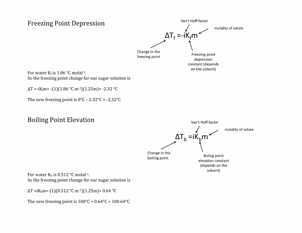
Thinking of cells as semipermeable membranes with stuff inside, the question becomes how much stuff is outside.  What matters for osmosis is not only the comparison only of solution to pure, but solutions of different concentrations to each other.  The free energy two solutions will be the same if they have the same concentration.  If not, the solvent will move to the solution with the higher concentration because it will have the lower free energy.  This gives rise to three situations.  First the concentration of stuff (salt, protein, small molecules…) outside the cell and inside the cell is the same.  Then the free energy is the same.  And the water going in is the same as the water going out.  This is the nice equilibrium case.   For cells we call this isotonic.  Next, is the case where the concentration outside is higher than inside the cell.  Now water leaves the cell to move to the higher concentration outside.  This is hypertonic and leads to dehydration (drying out) of the cells.  Finally, the outside is lower in concentration than inside.  This is hypotonic.  Now water moves into the cell.  Unless the cells can withstand very high pressures, they will burst.  Remember our solution before had an osmotic pressure of 28 atm!   Pressure can be high at even low concentrations.  Therefore putting cells in pure water will nearly always cause them to burst.