Lecture Notes

EE301 Signals and Systems I

Department of Electrical and Electronics Engineering

Middle East Technical University (METU)

Preface

These lecture notes were prepared with the purpose of helping the students to follow the lectures

more easily and efficiently. This course is a fast-paced course with a significant amount of material,

and to cover all of this material at a reasonable pace in the lectures, we intend to benefit from these

partially-complete lecture notes. In particular, we included important results, properties, comments

and examples, but left out most of the mathematics, derivations and solutions of examples, which

we do on the board and expect the students to write into the provided empty spaces in the notes.

We hope that this approach will reduce the note-taking burden on the students and will enable

more time to stress important concepts and discuss more examples.

These lecture notes were prepared using mainly our textbook titled ”Signals and Systems” by Alan

V. Oppenheim, Alan S. Willsky and S. Hamid Nawab, but also from handwritten notes of Fatih

Kamisli and A. Ozgur Yilmaz. Most figures and tables in the notes are also taken from the textbook.

This is the first version of the notes. Therefore the notes may contain errors and we also believe

there is room for improving the notes in many aspects. In this regard, we are open to feedback and

comments, especially from the students taking the course.

Fatih KamisliDecember 2nd, 2016.

1

Contents

1 Fundamental Concepts 6

1.1 Signals . . . . . . . . . . . . . . . . . . . . . . . . . . . . . . . . . . . . . . . . . . . . . . . . . . . . . . 7

1.1.1 Transformations of the independent variable of signals . . . . . . . . . . . . . . . . . . . . . . . 8

1.1.2 Periodic signals . . . . . . . . . . . . . . . . . . . . . . . . . . . . . . . . . . . . . . . . . . . . . 10

1.1.3 Even and Odd Signals . . . . . . . . . . . . . . . . . . . . . . . . . . . . . . . . . . . . . . . . . 10

1.1.4 DT Unit Impulse and Unit Step Sequences . . . . . . . . . . . . . . . . . . . . . . . . . . . . . 11

1.1.5 CT Unit Impulse and Unit Step Signals . . . . . . . . . . . . . . . . . . . . . . . . . . . . . . . 11

1.1.6 Brief review of complex algebra and arithmetic . . . . . . . . . . . . . . . . . . . . . . . . . . . 13

1.1.7 CT Complex Exponential Signals . . . . . . . . . . . . . . . . . . . . . . . . . . . . . . . . . . . 14

1.1.8 DT Complex Exponential Signals . . . . . . . . . . . . . . . . . . . . . . . . . . . . . . . . . . . 16

1.2 Systems and Basic System Properties . . . . . . . . . . . . . . . . . . . . . . . . . . . . . . . . . . . . 18

1.2.1 Memory Property . . . . . . . . . . . . . . . . . . . . . . . . . . . . . . . . . . . . . . . . . . . 19

1.2.2 Causality Property . . . . . . . . . . . . . . . . . . . . . . . . . . . . . . . . . . . . . . . . . . . 19

1.2.3 Invertibility . . . . . . . . . . . . . . . . . . . . . . . . . . . . . . . . . . . . . . . . . . . . . . . 20

1.2.4 Stability . . . . . . . . . . . . . . . . . . . . . . . . . . . . . . . . . . . . . . . . . . . . . . . . . 20

1.2.5 Time Invariance . . . . . . . . . . . . . . . . . . . . . . . . . . . . . . . . . . . . . . . . . . . . 21

1.2.6 Linearity . . . . . . . . . . . . . . . . . . . . . . . . . . . . . . . . . . . . . . . . . . . . . . . . 21

2 Linear Time-Invariant Systems 23

2.1 DT LTI Systems : The convolution sum . . . . . . . . . . . . . . . . . . . . . . . . . . . . . . . . . . . 24

2.1.1 Representation of DT Signals in terms of Impulses . . . . . . . . . . . . . . . . . . . . . . . . . 24

2.1.2 DT Unit Impulse Response and the Convolution Sum . . . . . . . . . . . . . . . . . . . . . . . 24

2.2 CT LTI Systems : The convolution integral . . . . . . . . . . . . . . . . . . . . . . . . . . . . . . . . . 26

2.2.1 Representation of CT Signals in terms of Impulses . . . . . . . . . . . . . . . . . . . . . . . . . 26

2.2.2 CT Unit Impulse Response and the Convolution Integral . . . . . . . . . . . . . . . . . . . . . 27

2.3 Properties of Convolution and LTI Systems . . . . . . . . . . . . . . . . . . . . . . . . . . . . . . . . . 29

2.3.1 Commutative property of convolution . . . . . . . . . . . . . . . . . . . . . . . . . . . . . . . . 30

2.3.2 Associative property of convolution . . . . . . . . . . . . . . . . . . . . . . . . . . . . . . . . . . 30

2.3.3 Distributive property of convolution . . . . . . . . . . . . . . . . . . . . . . . . . . . . . . . . . 30

2.3.4 Memory property in LTI systems . . . . . . . . . . . . . . . . . . . . . . . . . . . . . . . . . . . 31

2.3.5 Causality property in LTI systems . . . . . . . . . . . . . . . . . . . . . . . . . . . . . . . . . . 31

2.3.6 Stability property in LTI systems . . . . . . . . . . . . . . . . . . . . . . . . . . . . . . . . . . . 31

2.3.7 Invertibility property in LTI systems . . . . . . . . . . . . . . . . . . . . . . . . . . . . . . . . . 32

2.3.8 Unit Step Response of LTI systems . . . . . . . . . . . . . . . . . . . . . . . . . . . . . . . . . . 32

2.4 Systems Described by Differential and Difference Equations and Determining Their Impulse Responses 32

2.4.1 Determining The Impulse Response Using Initial Rest Conditions . . . . . . . . . . . . . . . . . 33

2.4.2 A Method for Differential Equations . . . . . . . . . . . . . . . . . . . . . . . . . . . . . . . . . 34

2.4.3 A Method for Difference Equations . . . . . . . . . . . . . . . . . . . . . . . . . . . . . . . . . . 35

2

2.4.4 Block Diagram Representations of First-Order Systems Described By Differential and Differ-

ence Equations . . . . . . . . . . . . . . . . . . . . . . . . . . . . . . . . . . . . . . . . . . . . . 36

3 Continuous-time Fourier Series 37

3.1 Response of LTI Systems to Complex Exponentials . . . . . . . . . . . . . . . . . . . . . . . . . . . . . 38

3.1.1 Eigenfunctions of LTI system . . . . . . . . . . . . . . . . . . . . . . . . . . . . . . . . . . . . . 38

3.2 Fourier series : Linear Combinations of Harmonically Related Complex Exponentials . . . . . . . . . . 39

3.3 Determination of CT Fourier Series Representation . . . . . . . . . . . . . . . . . . . . . . . . . . . . . 40

3.3.1 Coefficient matching approach . . . . . . . . . . . . . . . . . . . . . . . . . . . . . . . . . . . . 41

3.3.2 General approach . . . . . . . . . . . . . . . . . . . . . . . . . . . . . . . . . . . . . . . . . . . . 41

3.4 Existence and convergence of Fourier series . . . . . . . . . . . . . . . . . . . . . . . . . . . . . . . . . 42

3.5 Properties of Fourier Series . . . . . . . . . . . . . . . . . . . . . . . . . . . . . . . . . . . . . . . . . . 44

3.5.1 Linearity property . . . . . . . . . . . . . . . . . . . . . . . . . . . . . . . . . . . . . . . . . . . 44

3.5.2 Symmetry with real signals . . . . . . . . . . . . . . . . . . . . . . . . . . . . . . . . . . . . . . 44

3.5.3 Alternative forms of FS representation for real signals . . . . . . . . . . . . . . . . . . . . . . . 44

3.5.4 Even and odd signals . . . . . . . . . . . . . . . . . . . . . . . . . . . . . . . . . . . . . . . . . . 45

3.5.5 FS coefficients of manipulated CT periodic signals . . . . . . . . . . . . . . . . . . . . . . . . . 45

3.5.6 Response of LTI systems to signals with FS representation . . . . . . . . . . . . . . . . . . . . 46

3.5.7 Other properties of CTFS representation . . . . . . . . . . . . . . . . . . . . . . . . . . . . . . 47

4 Continuous-time Fourier Transform 48

4.1 The Fourier Transform Representation of CT Aperiodic Signals . . . . . . . . . . . . . . . . . . . . . . 49

4.1.1 Intuition behind Fourier transform . . . . . . . . . . . . . . . . . . . . . . . . . . . . . . . . . . 49

4.1.2 Formal development of Fourier transform . . . . . . . . . . . . . . . . . . . . . . . . . . . . . . 49

4.2 Convergence of Fourier Transform . . . . . . . . . . . . . . . . . . . . . . . . . . . . . . . . . . . . . . 51

4.3 Examples of CT Fourier transforms . . . . . . . . . . . . . . . . . . . . . . . . . . . . . . . . . . . . . . 51

4.4 Response of LTI systems to complex exponentials (revisited) . . . . . . . . . . . . . . . . . . . . . . . 53

4.5 Fourier transform of periodic signals . . . . . . . . . . . . . . . . . . . . . . . . . . . . . . . . . . . . . 54

4.6 Properties of the Fourier Transform . . . . . . . . . . . . . . . . . . . . . . . . . . . . . . . . . . . . . 56

4.6.1 Linearity . . . . . . . . . . . . . . . . . . . . . . . . . . . . . . . . . . . . . . . . . . . . . . . . 56

4.6.2 Time Shift . . . . . . . . . . . . . . . . . . . . . . . . . . . . . . . . . . . . . . . . . . . . . . . 56

4.6.3 Time and Frequency Scaling . . . . . . . . . . . . . . . . . . . . . . . . . . . . . . . . . . . . . 57

4.6.4 Conjugation and Conjugate Symmetry . . . . . . . . . . . . . . . . . . . . . . . . . . . . . . . . 57

4.6.5 Differentiation and Integration . . . . . . . . . . . . . . . . . . . . . . . . . . . . . . . . . . . . 59

4.6.6 Duality . . . . . . . . . . . . . . . . . . . . . . . . . . . . . . . . . . . . . . . . . . . . . . . . . 60

4.6.7 Parseval’s Relation . . . . . . . . . . . . . . . . . . . . . . . . . . . . . . . . . . . . . . . . . . . 60

4.6.8 Convolution Property . . . . . . . . . . . . . . . . . . . . . . . . . . . . . . . . . . . . . . . . . 61

4.6.9 Modulation (Multiplication) property . . . . . . . . . . . . . . . . . . . . . . . . . . . . . . . . 63

4.6.10 Table of properties of CT FT . . . . . . . . . . . . . . . . . . . . . . . . . . . . . . . . . . . . . 64

4.6.11 Table of basic signals and their CT FT and FS . . . . . . . . . . . . . . . . . . . . . . . . . . . 65

4.7 Some applications of Fourier transform . . . . . . . . . . . . . . . . . . . . . . . . . . . . . . . . . . . . 66

4.7.1 Amplitude Modulation (AM) . . . . . . . . . . . . . . . . . . . . . . . . . . . . . . . . . . . . . 66

4.7.2 Frequency Division Multiplexing (FDM) . . . . . . . . . . . . . . . . . . . . . . . . . . . . . . . 68

4.7.3 Single Sideband Modulation (SSB) . . . . . . . . . . . . . . . . . . . . . . . . . . . . . . . . . . 69

5 Discrete-time Fourier Series and Transform 70

5.1 DT Fourier Series . . . . . . . . . . . . . . . . . . . . . . . . . . . . . . . . . . . . . . . . . . . . . . . . 71

5.1.1 Response of DT LTI Systems to Complex Exponentials . . . . . . . . . . . . . . . . . . . . . . 71

5.1.2 DT Fourier series representation of periodic DT signals . . . . . . . . . . . . . . . . . . . . . . 72

3

5.2 DT Fourier Transform . . . . . . . . . . . . . . . . . . . . . . . . . . . . . . . . . . . . . . . . . . . . . 75

5.2.1 Intuition and formal development of DT Fourier transform . . . . . . . . . . . . . . . . . . . . 75

5.2.2 Convergence of DT Fourier transform . . . . . . . . . . . . . . . . . . . . . . . . . . . . . . . . 76

5.2.3 Examples of DT Fourier transform . . . . . . . . . . . . . . . . . . . . . . . . . . . . . . . . . . 76

5.2.4 Response of LTI systems to complex exponentials (revisited) . . . . . . . . . . . . . . . . . . . 77

5.2.5 DT Fourier transform of periodic signals . . . . . . . . . . . . . . . . . . . . . . . . . . . . . . . 78

5.3 Properties of DT Fourier series and transform . . . . . . . . . . . . . . . . . . . . . . . . . . . . . . . . 80

5.3.1 Periodicity . . . . . . . . . . . . . . . . . . . . . . . . . . . . . . . . . . . . . . . . . . . . . . . 80

5.3.2 Linearity . . . . . . . . . . . . . . . . . . . . . . . . . . . . . . . . . . . . . . . . . . . . . . . . 80

5.3.3 Time Shifting and Frequency Shifting . . . . . . . . . . . . . . . . . . . . . . . . . . . . . . . . 80

5.3.4 Conjugation and Conjugate Symmetry . . . . . . . . . . . . . . . . . . . . . . . . . . . . . . . . 81

5.3.5 Differencing and Accumulation . . . . . . . . . . . . . . . . . . . . . . . . . . . . . . . . . . . . 82

5.3.6 Time Reversal . . . . . . . . . . . . . . . . . . . . . . . . . . . . . . . . . . . . . . . . . . . . . 82

5.3.7 Differentiation in Frequency . . . . . . . . . . . . . . . . . . . . . . . . . . . . . . . . . . . . . . 82

5.3.8 Time Expansion . . . . . . . . . . . . . . . . . . . . . . . . . . . . . . . . . . . . . . . . . . . . 82

5.3.9 Parseval’s Relation . . . . . . . . . . . . . . . . . . . . . . . . . . . . . . . . . . . . . . . . . . . 84

5.3.10 Convolution Property . . . . . . . . . . . . . . . . . . . . . . . . . . . . . . . . . . . . . . . . . 85

5.3.11 Multiplication property . . . . . . . . . . . . . . . . . . . . . . . . . . . . . . . . . . . . . . . . 86

5.3.12 Table of properties of DT FT and FS . . . . . . . . . . . . . . . . . . . . . . . . . . . . . . . . 87

5.3.13 Table of basic signals and their DT FT and FS . . . . . . . . . . . . . . . . . . . . . . . . . . . 87

6 Sampling 90

6.1 Representation of CT signals by its samples : the sampling theorem . . . . . . . . . . . . . . . . . . . 91

6.1.1 Impulse-train sampling . . . . . . . . . . . . . . . . . . . . . . . . . . . . . . . . . . . . . . . . . 91

6.1.2 Sampling with a zero-order hold . . . . . . . . . . . . . . . . . . . . . . . . . . . . . . . . . . . 94

6.2 Effect of undersampling . . . . . . . . . . . . . . . . . . . . . . . . . . . . . . . . . . . . . . . . . . . . 95

6.3 DT processing of CT signals . . . . . . . . . . . . . . . . . . . . . . . . . . . . . . . . . . . . . . . . . . 95

6.3.1 C/D conversion . . . . . . . . . . . . . . . . . . . . . . . . . . . . . . . . . . . . . . . . . . . . . 96

6.3.2 D/C conversion . . . . . . . . . . . . . . . . . . . . . . . . . . . . . . . . . . . . . . . . . . . . . 96

7 The Z-transform 98

7.1 The Z transform and its region of convergence (ROC) . . . . . . . . . . . . . . . . . . . . . . . . . . . 99

7.2 Properties of ROC . . . . . . . . . . . . . . . . . . . . . . . . . . . . . . . . . . . . . . . . . . . . . . . 102

7.3 Inversion of Z transforms . . . . . . . . . . . . . . . . . . . . . . . . . . . . . . . . . . . . . . . . . . . 105

7.4 Properties of Z transform . . . . . . . . . . . . . . . . . . . . . . . . . . . . . . . . . . . . . . . . . . . 106

7.4.1 Linearity . . . . . . . . . . . . . . . . . . . . . . . . . . . . . . . . . . . . . . . . . . . . . . . . 106

7.4.2 Time Shift . . . . . . . . . . . . . . . . . . . . . . . . . . . . . . . . . . . . . . . . . . . . . . . 107

7.4.3 Scaling in z domain (Frequency shifting) . . . . . . . . . . . . . . . . . . . . . . . . . . . . . . . 107

7.4.4 Time Reversal . . . . . . . . . . . . . . . . . . . . . . . . . . . . . . . . . . . . . . . . . . . . . 107

7.4.5 Conjugation . . . . . . . . . . . . . . . . . . . . . . . . . . . . . . . . . . . . . . . . . . . . . . . 107

7.4.6 Convolution . . . . . . . . . . . . . . . . . . . . . . . . . . . . . . . . . . . . . . . . . . . . . . . 108

7.4.7 Differentiation . . . . . . . . . . . . . . . . . . . . . . . . . . . . . . . . . . . . . . . . . . . . . 108

7.4.8 The initial value theorem . . . . . . . . . . . . . . . . . . . . . . . . . . . . . . . . . . . . . . . 108

7.4.9 Table of Z transform properties and some common z transform pairs . . . . . . . . . . . . . . . 109

7.5 LTI Systems and the Z transform . . . . . . . . . . . . . . . . . . . . . . . . . . . . . . . . . . . . . . . 110

7.5.1 Causality . . . . . . . . . . . . . . . . . . . . . . . . . . . . . . . . . . . . . . . . . . . . . . . . 110

7.5.2 Stability . . . . . . . . . . . . . . . . . . . . . . . . . . . . . . . . . . . . . . . . . . . . . . . . . 111

4

8 The Laplace transform 113

8.1 The Laplace transform and its region of convergence (ROC) . . . . . . . . . . . . . . . . . . . . . . . . 113

8.2 Properties of ROC . . . . . . . . . . . . . . . . . . . . . . . . . . . . . . . . . . . . . . . . . . . . . . . 117

8.3 Inversion of Laplace transforms . . . . . . . . . . . . . . . . . . . . . . . . . . . . . . . . . . . . . . . . 119

8.4 Properties of Laplace transform . . . . . . . . . . . . . . . . . . . . . . . . . . . . . . . . . . . . . . . . 120

8.4.1 Linearity . . . . . . . . . . . . . . . . . . . . . . . . . . . . . . . . . . . . . . . . . . . . . . . . 120

8.4.2 Time Shift . . . . . . . . . . . . . . . . . . . . . . . . . . . . . . . . . . . . . . . . . . . . . . . 120

8.4.3 Frequency Shift . . . . . . . . . . . . . . . . . . . . . . . . . . . . . . . . . . . . . . . . . . . . . 121

8.4.4 Time Scaling . . . . . . . . . . . . . . . . . . . . . . . . . . . . . . . . . . . . . . . . . . . . . . 121

8.4.5 Conjugation . . . . . . . . . . . . . . . . . . . . . . . . . . . . . . . . . . . . . . . . . . . . . . . 121

8.4.6 Convolution . . . . . . . . . . . . . . . . . . . . . . . . . . . . . . . . . . . . . . . . . . . . . . . 121

8.4.7 Differentiation in s domain . . . . . . . . . . . . . . . . . . . . . . . . . . . . . . . . . . . . . . 121

8.4.8 Differentiation in time domain . . . . . . . . . . . . . . . . . . . . . . . . . . . . . . . . . . . . 122

8.4.9 Integration in time domain . . . . . . . . . . . . . . . . . . . . . . . . . . . . . . . . . . . . . . 122

8.4.10 Initial and Final Value Theorem . . . . . . . . . . . . . . . . . . . . . . . . . . . . . . . . . . . 122

8.4.11 Table of Laplace transform properties and common Laplace transform pairs . . . . . . . . . . . 123

8.5 LTI Systems and the Laplace transform . . . . . . . . . . . . . . . . . . . . . . . . . . . . . . . . . . . 124

8.5.1 Causality . . . . . . . . . . . . . . . . . . . . . . . . . . . . . . . . . . . . . . . . . . . . . . . . 124

8.5.2 Stability . . . . . . . . . . . . . . . . . . . . . . . . . . . . . . . . . . . . . . . . . . . . . . . . . 125

5

Chapter 1

Fundamental Concepts

Contents

1.1 Signals . . . . . . . . . . . . . . . . . . . . . . . . . . . . . . . . . . . . . . . . . . . . . . . . 7

1.1.1 Transformations of the independent variable of signals . . . . . . . . . . . . . . . . . . . . . 8

1.1.2 Periodic signals . . . . . . . . . . . . . . . . . . . . . . . . . . . . . . . . . . . . . . . . . . . 10

1.1.3 Even and Odd Signals . . . . . . . . . . . . . . . . . . . . . . . . . . . . . . . . . . . . . . . 10

1.1.4 DT Unit Impulse and Unit Step Sequences . . . . . . . . . . . . . . . . . . . . . . . . . . . 11

1.1.5 CT Unit Impulse and Unit Step Signals . . . . . . . . . . . . . . . . . . . . . . . . . . . . . 11

1.1.6 Brief review of complex algebra and arithmetic . . . . . . . . . . . . . . . . . . . . . . . . . 13

1.1.7 CT Complex Exponential Signals . . . . . . . . . . . . . . . . . . . . . . . . . . . . . . . . . 14

1.1.8 DT Complex Exponential Signals . . . . . . . . . . . . . . . . . . . . . . . . . . . . . . . . . 16

1.2 Systems and Basic System Properties . . . . . . . . . . . . . . . . . . . . . . . . . . . . . 18

1.2.1 Memory Property . . . . . . . . . . . . . . . . . . . . . . . . . . . . . . . . . . . . . . . . . 19

1.2.2 Causality Property . . . . . . . . . . . . . . . . . . . . . . . . . . . . . . . . . . . . . . . . . 19

1.2.3 Invertibility . . . . . . . . . . . . . . . . . . . . . . . . . . . . . . . . . . . . . . . . . . . . . 20

1.2.4 Stability . . . . . . . . . . . . . . . . . . . . . . . . . . . . . . . . . . . . . . . . . . . . . . . 20

1.2.5 Time Invariance . . . . . . . . . . . . . . . . . . . . . . . . . . . . . . . . . . . . . . . . . . 21

1.2.6 Linearity . . . . . . . . . . . . . . . . . . . . . . . . . . . . . . . . . . . . . . . . . . . . . . 21

What is signal processing ? Watch the following videos for a great description of signal processing

and some great examples of its applications :

• https://www.youtube.com/watch?v=EErkgr1MWw0

(Search youtube for : What is Signal Processing?)

• https://www.youtube.com/watch?v=mexN6d8QF9o

(Search youtube for : Signal Processing and Machine Learning)

This chapter introduces basic signals, systems and their properties.

6

1.1 Signals

Definition 1 A signal is the variation of a physical, or non-physical, quantity with respect to one

or more independent variable(s). Signals typically carry information that is somehow relevant for

some purpose.

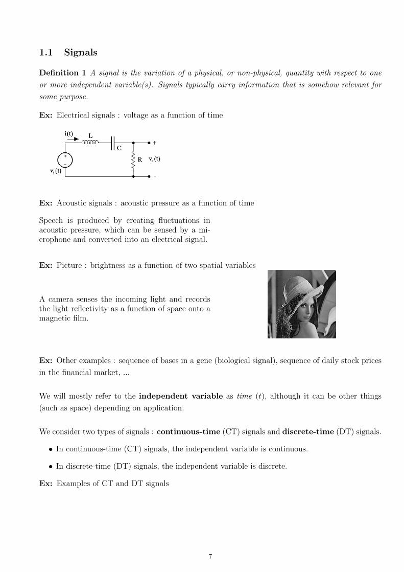
Ex: Electrical signals : voltage as a function of time

Ex: Acoustic signals : acoustic pressure as a function of time

Speech is produced by creating fluctuations inacoustic pressure, which can be sensed by a mi-crophone and converted into an electrical signal.

Ex: Picture : brightness as a function of two spatial variables

A camera senses the incoming light and recordsthe light reflectivity as a function of space onto amagnetic film.

Ex: Other examples : sequence of bases in a gene (biological signal), sequence of daily stock prices

in the financial market, ...

We will mostly refer to the independent variable as time (t), although it can be other things

(such as space) depending on application.

We consider two types of signals : continuous-time (CT) signals and discrete-time (DT) signals.

• In continuous-time (CT) signals, the independent variable is continuous.

• In discrete-time (DT) signals, the independent variable is discrete.

Ex: Examples of CT and DT signals

7

Note : DT signals are undefined at values other than the specified discrete values.

Independent variables can be 1-D, 2-D, 3-D,...

Ex:

Speech signal :

Image signal :

Video signal :

Throughout the course, following notation is used to represent CT and DT signals :

CT signals :

DT signals :

Most physical signals are CT, but not all. A DT signal may be obtained from phenomena

• that is inherently discrete (as in the ’people attending lecture’ example)

• that is obtained by taking samples from a CT signal (as in the ’blood pressure’ example).

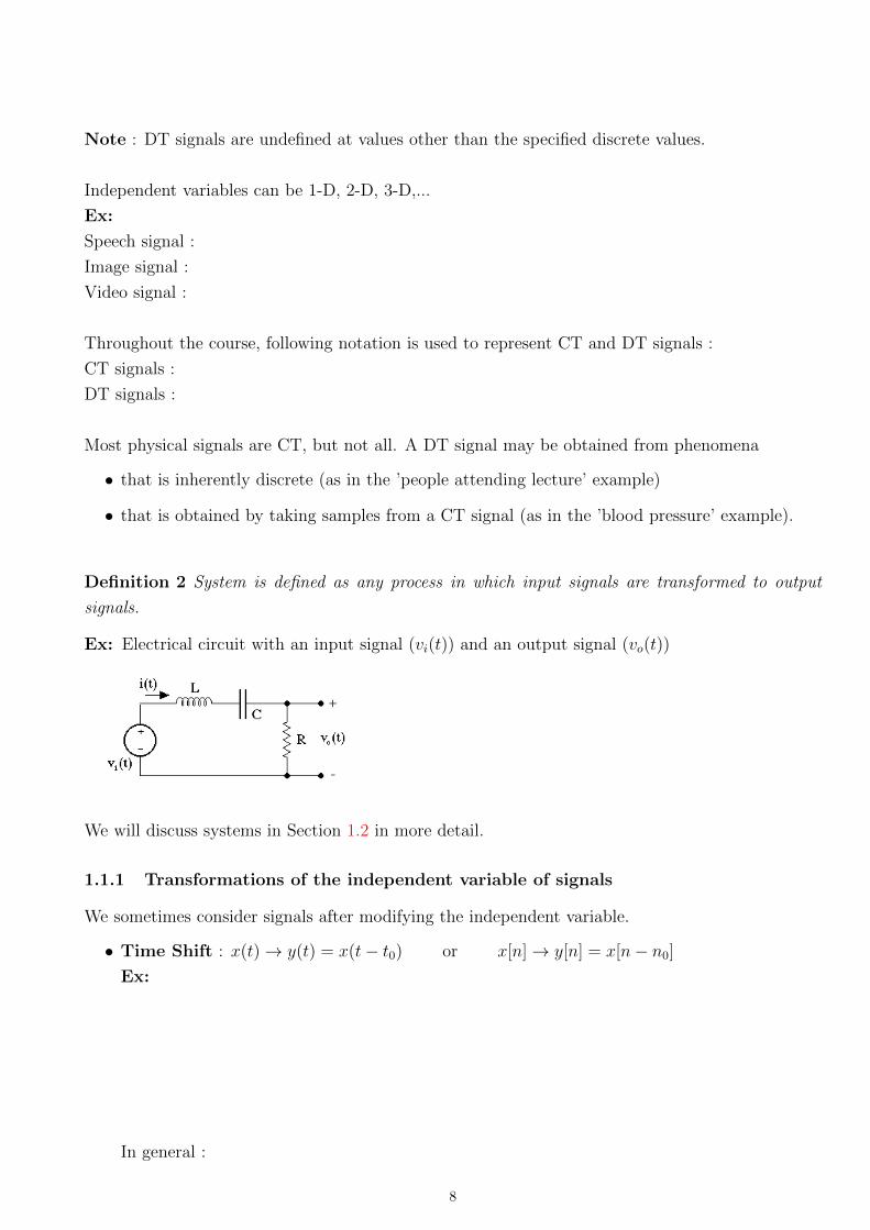
Definition 2 System is defined as any process in which input signals are transformed to output

signals.

Ex: Electrical circuit with an input signal (vi(t)) and an output signal (vo(t))

We will discuss systems in Section 1.2 in more detail.

1.1.1 Transformations of the independent variable of signals

We sometimes consider signals after modifying the independent variable.

• Time Shift : x(t)→ y(t) = x(t− t0) or x[n]→ y[n] = x[n− n0]

Ex:

In general :

8

• Time Reversal (Reflection) : x(t)→ y(t) = x(−t) or x[n]→ y[n] = x[−n]

Ex:

• Time Scaling : x(t)→ y(t) = x(at), a ∈ R or x[n]→ y[n] = x[bn], b ∈ ZEx:

In general :

Note : x(at) is always defined for a ε R. The same is not true for x[bn], unless b ∈ Z, i.e. b is an

integer.

Ex: For x[n] : x[2n] x[√

2n] x[n2]

Ex: Find and plot y(t) = x(−t+ 1) for

9

Ex: Find and plot y[n] = x[−2n+ 1] for

1.1.2 Periodic signals

A periodic CT signal x(t) has the property that there is a period T ∈ R+ for which

x(t) =

It is said that x(t) is periodic with T .

Periodicity is defined similarly for DT signals :

Ex:

Note : If x(t) is periodic with T then it is also periodic with 2T, 3T, 4T, ..., i.e. k ·T, k ∈ Z+.(Same

holds for DT signals.)

Fundamental period T0 of x(t) (N0 of x[n]) is the smallest positive T (N) for which x(t) (x[n])

is periodic, i.e. the above equalities hold.

1.1.3 Even and Odd Signals

A CT signal is even if x(t) = x(−t) ∀t. (In DT: x[−n] = x[n] ∀n)

A CT signal is odd if x(t) = −x(−t) ∀t. (In DT: x[n] = −x[−n] ∀n)

Ex:

Any signal x(t) (x[n]) can be written uniquely as a sum of its even and odd part :

10

In the next subsections, we will discuss some basic CT and DT signals, in particular,

• DT and CT unit impulse and step signals and

• CT and DT complex exponential signals.

1.1.4 DT Unit Impulse and Unit Step Sequences

DT Unit Impulse signal

δ[n] =

1, n = 0

0, n 6= 0.

DT Unit Step signal

u[n] =

1, n ≥ 0

0, n < 0.

Relations between δ[n] and u[n] and some properties

• δ[n] =

• u[n] =

•∑k2

k=k1δ[k] =

• x[n]δ[n− n0] =

•∑k2

k=k1x[k]δ[k − n0] =

Ex: : Compute the following expressions∑k2

i=k1x[i]δ[i]

u[n] =∑n

i=−∞ δ[i] (show it)

1.1.5 CT Unit Impulse and Unit Step Signals

To study the CT unit step (u(t)) and impulse (δ(t)) signals, let us first examine their approximations

u∆(t) and δ∆(t) :

Note that u∆(t) and δ∆(t) are related by :

11

As ∆→ 0, u(t) and δ(t) are obtained, which still satisfy the above relations :

CT Unit Step signal u(t)

u(t) =

0, t < 0

1, t > 0.

CT Unit Impulse signal δ(t)

δ(t) is not defined directly as in many other functions, but by its properties :

• δ(t) = ddtu(t)

• δ(t) = 0, t 6= 0 and

•∫ t2τ=t1

δ(τ)dτ =

• u(t) =∫ t−∞ δ(τ)dτ (Running Sum Interpretation)

• x(t)δ(t− t0) =

•∫ t2τ=t1

x(τ)δ(τ − t0)dτ =

Ex: : Compute the following expressions∫∞σ=0

δ(t− σ)dσ =∫ tτ=−∞ x(τ)δ(τ)dτ =

Ex: (Square type signal)

12

1.1.6 Brief review of complex algebra and arithmetic

Rectangular (cartesian) form z = x+ j · y

Euler’s relation : ejθ =

Polar form : z = r · ejθ

Components of rectangular and polar form are related :

Complex conjugate of a complex number z is represented with z∗ :

Complex arithmetic :

13

1.1.7 CT Complex Exponential Signals

The CT complex exponential signal is of the form

x(t) = Ceat

where C and a are in general complex numbers.

Real Exponential Signals

If C and a are real numbers, real exponential signals are obtained.

• a > 0, growing exponential:

• a < 0, decaying exponential:

Periodic Complex Exponential and Sinusoidal Signals

If a is purely imaginary, periodic complex exponentials are obtained.

Notes:

• Fundamental period of x(t) = ejω0t is T0 =2π

ω0

• ejw0t and e−jw0t have the same fundamental period → T0 =2π

|ω0|

• The sinusoidal signals xa(t) = A cos(ω0t) and xb(t) = A sin(ω0t) are closely related to ejω0t :

• Let’s define fundamental frequency as |ω0| =2π

T0

(|ω0| represents rate of oscillation)

14

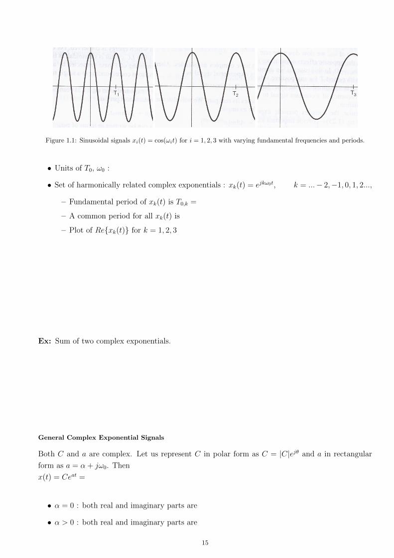
Figure 1.1: Sinusoidal signals xi(t) = cos(ωit) for i = 1, 2, 3 with varying fundamental frequencies and periods.

• Units of T0, ω0 :

• Set of harmonically related complex exponentials : xk(t) = ejkω0t, k = ...− 2,−1, 0, 1, 2...,

– Fundamental period of xk(t) is T0,k =

– A common period for all xk(t) is

– Plot of Rexk(t) for k = 1, 2, 3

Ex: Sum of two complex exponentials.

General Complex Exponential Signals

Both C and a are complex. Let us represent C in polar form as C = |C|ejθ and a in rectangular

form as a = α + jω0. Then

x(t) = Ceat =

• α = 0 : both real and imaginary parts are

• α > 0 : both real and imaginary parts are

15

• α < 0 : both real and imaginary parts are

Ex: x(t) = 2e(2+jω0)t

Ex: x(t) = 2e(−1+jω0)t

1.1.8 DT Complex Exponential Signals

The DT complex exponential signal is of the form

x[n] = Cαn or x[n] = Ceβn (where α = eβ)

where C and α are in general complex numbers.

Real Exponential Signals

If C and a are real numbers, real exponential signals are obtained with various behavior.

Ex:

Sinusoidal Signals

If β is purely imaginary (i.e. |α| = 1), DT sinusoidals are obtained. Consider x[n] = CejΩ0n.

16

General Complex Exponential Signals

If β = α + j · Ω, then damped sinusoidals (decaying or growing) are obtained (see textbook for

details.)

Periodicity Properties of DT Complex Exponential Signals

Although there are many similarities between CT and DT signals, there are also important dif-

ferences. One of these is the different properties of complex exponential signals x(t) = ejω0t and

x[n] = ejΩ0n.

We discussed x(t) = ejω0t previously and we can identify two important properties of it :

• it is periodic for any value of ω0 and its fundamental period is T0 =2π

ω0

• the larger the magnitude of ω0, the higher the rate of oscillation (i.e. frequency) in the signals.

Both of the above properties are different for x[n] = ejΩ0n:

• x[n] = ejω0n is periodic only if Ω0 can be written in the form Ω0 = 2πmN

for some integers

N > 0, and m.

• x[n] = ejΩ0n does not have a continually increasing rate of oscillation as we increase the

magnitude of Ω0. In particular, x1[n] = ejΩ0n is equal to x2[n] = ej(Ω0+k2π)n, k ∈ Z.

Ex: Which of the following are periodic ? For each, find fundamental period if periodic.

x(t) = ej2t x[n] = ej2n x[n] = ejπn x[n] = cos(πn)

17

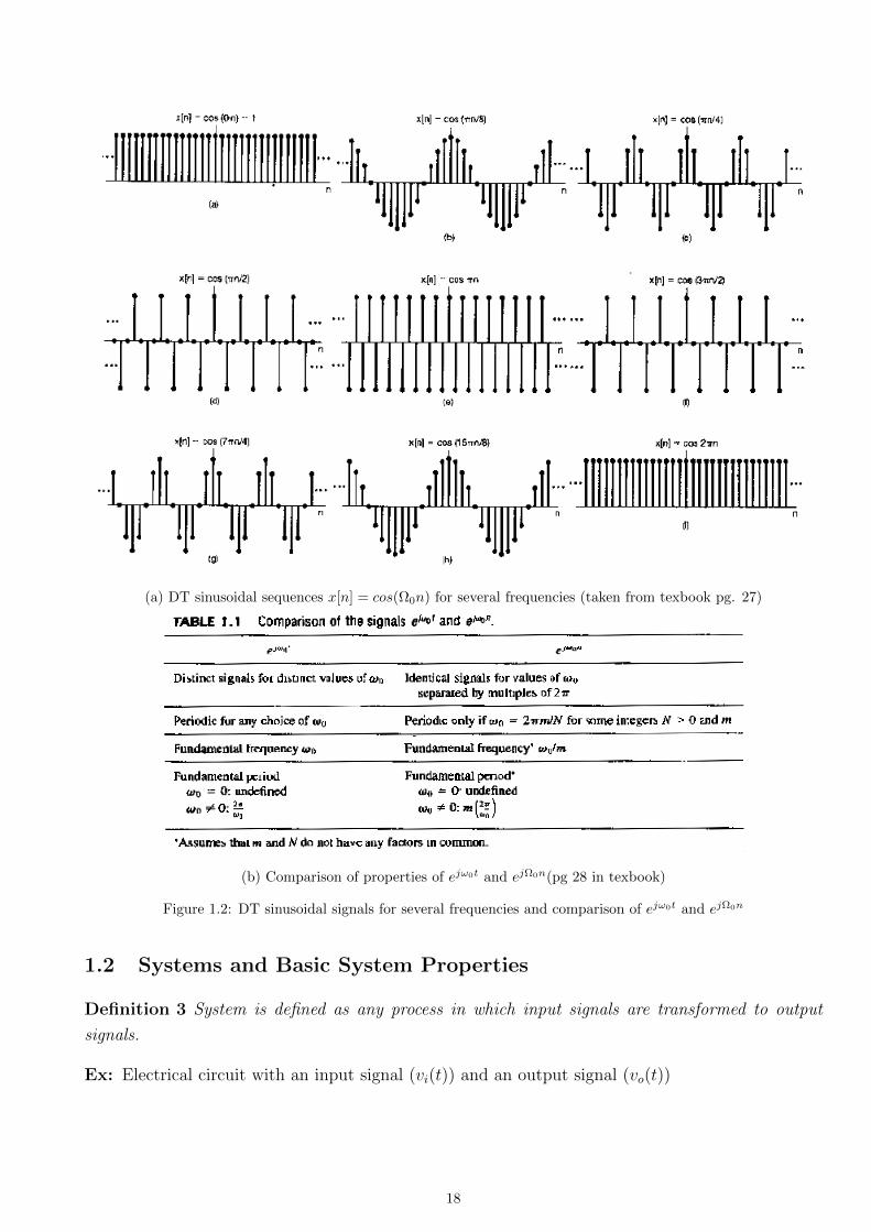
(a) DT sinusoidal sequences x[n] = cos(Ω0n) for several frequencies (taken from texbook pg. 27)

(b) Comparison of properties of ejω0t and ejΩ0n(pg 28 in texbook)

Figure 1.2: DT sinusoidal signals for several frequencies and comparison of ejω0t and ejΩ0n

1.2 Systems and Basic System Properties

Definition 3 System is defined as any process in which input signals are transformed to output

signals.

Ex: Electrical circuit with an input signal (vi(t)) and an output signal (vo(t))

18

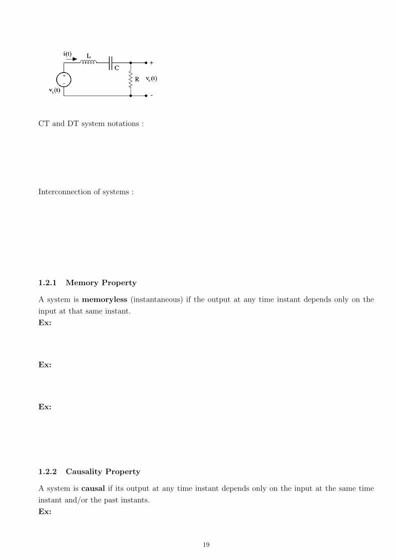
CT and DT system notations :

Interconnection of systems :

1.2.1 Memory Property

A system is memoryless (instantaneous) if the output at any time instant depends only on the

input at that same instant.

Ex:

Ex:

Ex:

1.2.2 Causality Property

A system is causal if its output at any time instant depends only on the input at the same time

instant and/or the past instants.

Ex:

19

Ex:

Ex:

1.2.3 Invertibility

A system is invertible if distinct inputs lead to distinct outputs. If a system is invertible, then a

corresponding inverse system exists such that

Ex:

Ex:

(You are not responsible from this property as other sections do not discuss it, but see textbook for

details and examples if interested.)

1.2.4 Stability

A system is stable if it produces bounded output signal for any bounded input signal.

Bounded signal : Its value at any time is bounded by two finite values.

Ex:

Ex:

Ex:

20

Ex:

1.2.5 Time Invariance

A system is time-invariant if a time shift of the input causes a time shift at the output by the

same amount for any input. In other words,

Ex:

Ex:

Ex:

Ex:

1.2.6 Linearity

A linear system must satisfy the superposition property, which is as follows :

21

Ex:

Ex:

Ex:

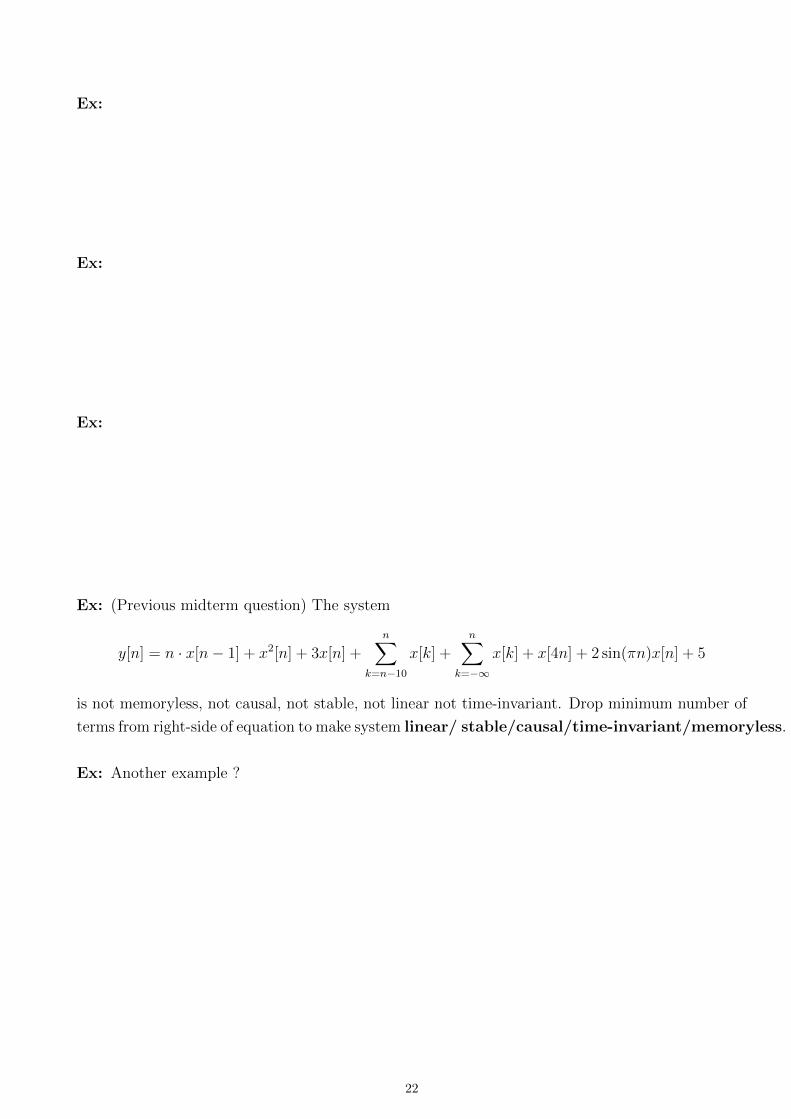
Ex: (Previous midterm question) The system

y[n] = n · x[n− 1] + x2[n] + 3x[n] +n∑

k=n−10

x[k] +n∑

k=−∞

x[k] + x[4n] + 2 sin(πn)x[n] + 5

is not memoryless, not causal, not stable, not linear not time-invariant. Drop minimum number of

terms from right-side of equation to make system linear/ stable/causal/time-invariant/memoryless.

Ex: Another example ?

22

Chapter 2

Linear Time-Invariant Systems

Contents

2.1 DT LTI Systems : The convolution sum . . . . . . . . . . . . . . . . . . . . . . . . . . . . 24

2.1.1 Representation of DT Signals in terms of Impulses . . . . . . . . . . . . . . . . . . . . . . . 24

2.1.2 DT Unit Impulse Response and the Convolution Sum . . . . . . . . . . . . . . . . . . . . . 24

2.2 CT LTI Systems : The convolution integral . . . . . . . . . . . . . . . . . . . . . . . . . 26

2.2.1 Representation of CT Signals in terms of Impulses . . . . . . . . . . . . . . . . . . . . . . . 26

2.2.2 CT Unit Impulse Response and the Convolution Integral . . . . . . . . . . . . . . . . . . . 27

2.3 Properties of Convolution and LTI Systems . . . . . . . . . . . . . . . . . . . . . . . . . 29

2.3.1 Commutative property of convolution . . . . . . . . . . . . . . . . . . . . . . . . . . . . . . 30

2.3.2 Associative property of convolution . . . . . . . . . . . . . . . . . . . . . . . . . . . . . . . . 30

2.3.3 Distributive property of convolution . . . . . . . . . . . . . . . . . . . . . . . . . . . . . . . 30

2.3.4 Memory property in LTI systems . . . . . . . . . . . . . . . . . . . . . . . . . . . . . . . . . 31

2.3.5 Causality property in LTI systems . . . . . . . . . . . . . . . . . . . . . . . . . . . . . . . . 31

2.3.6 Stability property in LTI systems . . . . . . . . . . . . . . . . . . . . . . . . . . . . . . . . . 31

2.3.7 Invertibility property in LTI systems . . . . . . . . . . . . . . . . . . . . . . . . . . . . . . . 32

2.3.8 Unit Step Response of LTI systems . . . . . . . . . . . . . . . . . . . . . . . . . . . . . . . . 32

2.4 Systems Described by Differential and Difference Equations and Determining Their

Impulse Responses . . . . . . . . . . . . . . . . . . . . . . . . . . . . . . . . . . . . . . . . . 32

2.4.1 Determining The Impulse Response Using Initial Rest Conditions . . . . . . . . . . . . . . . 33

2.4.2 A Method for Differential Equations . . . . . . . . . . . . . . . . . . . . . . . . . . . . . . . 34

2.4.3 A Method for Difference Equations . . . . . . . . . . . . . . . . . . . . . . . . . . . . . . . . 35

2.4.4 Block Diagram Representations of First-Order Systems Described By Differential and Dif-

ference Equations . . . . . . . . . . . . . . . . . . . . . . . . . . . . . . . . . . . . . . . . . . 36

Two of the important system properties discussed in the previous chapter are linearity and time-

invariance. Systems possessing these two properties are called Linear Time-Invariant (LTI) systems

and LTI systems are very important for system and signal analysis for two reasons:

• many physical systems are LTI, and

• powerful mathematical tools have been developed to study/analyze/design LTI systems.

This chapter discusses LTI systems in detail.

23

2.1 DT LTI Systems : The convolution sum

2.1.1 Representation of DT Signals in terms of Impulses

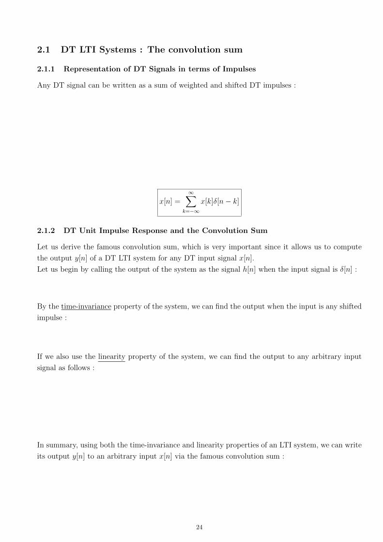
Any DT signal can be written as a sum of weighted and shifted DT impulses :

x[n] =∞∑

k=−∞

x[k]δ[n− k]

2.1.2 DT Unit Impulse Response and the Convolution Sum

Let us derive the famous convolution sum, which is very important since it allows us to compute

the output y[n] of a DT LTI system for any DT input signal x[n].

Let us begin by calling the output of the system as the signal h[n] when the input signal is δ[n] :

By the time-invariance property of the system, we can find the output when the input is any shifted

impulse :

If we also use the linearity property of the system, we can find the output to any arbitrary input

signal as follows :

In summary, using both the time-invariance and linearity properties of an LTI system, we can write

its output y[n] to an arbitrary input x[n] via the famous convolution sum :

24

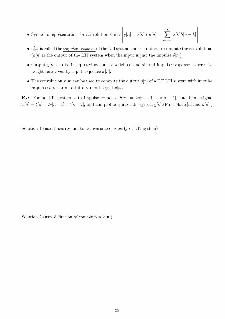
• Symbolic representation for convolution sum : y[n] = x[n] ∗ h[n] =∞∑

k=−∞

x[k]h[n− k]

• h[n] is called the impulse response of the LTI system and is required to compute the convolution.

(h[n] is the output of the LTI system when the input is just the impulse δ[n])

• Output y[n] can be interpreted as sum of weighted and shifted impulse responses where the

weights are given by input sequence x[n].

• The convolution sum can be used to compute the output y[n] of a DT LTI system with impulse

response h[n] for an arbitrary input signal x[n].

Ex: For an LTI system with impulse response h[n] = 2δ[n + 1] + δ[n − 1], and input signal

x[n] = δ[n] + 2δ[n− 1] + δ[n− 2], find and plot output of the system y[n].(First plot x[n] and h[n].)

Solution 1 (uses linearity and time-invariance property of LTI system)

Solution 2 (uses definition of convolution sum)

25

.

Ex: Let x[n] = αnu[n] (0 < α < 1) and h[n] = u[n]. Find y[n] = x[n] ∗ h[n].

2.2 CT LTI Systems : The convolution integral

2.2.1 Representation of CT Signals in terms of Impulses

Consider a staircase approximation to a CT signal x(t) :

26

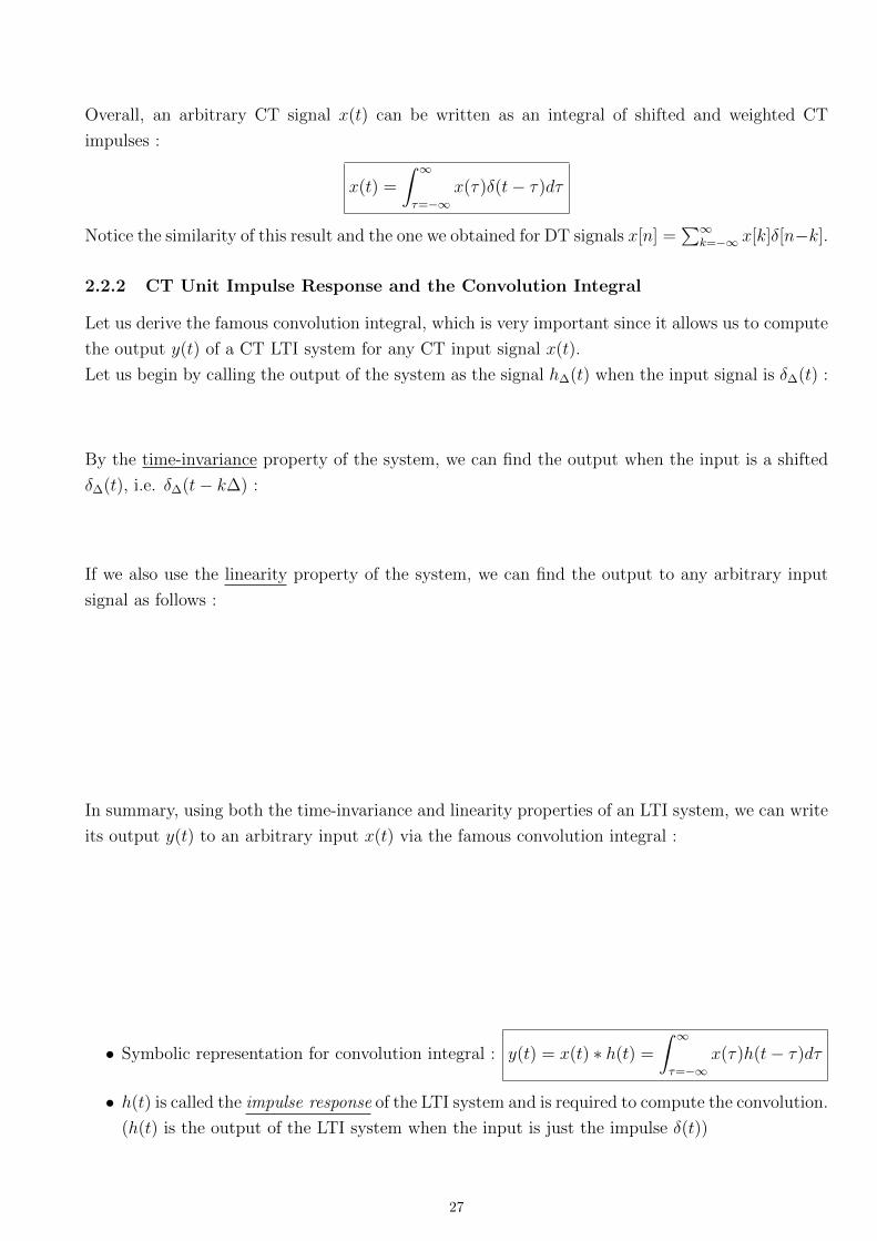
Overall, an arbitrary CT signal x(t) can be written as an integral of shifted and weighted CT

impulses :

x(t) =

∫ ∞τ=−∞

x(τ)δ(t− τ)dτ

Notice the similarity of this result and the one we obtained for DT signals x[n] =∑∞

k=−∞ x[k]δ[n−k].

2.2.2 CT Unit Impulse Response and the Convolution Integral

Let us derive the famous convolution integral, which is very important since it allows us to compute

the output y(t) of a CT LTI system for any CT input signal x(t).

Let us begin by calling the output of the system as the signal h∆(t) when the input signal is δ∆(t) :

By the time-invariance property of the system, we can find the output when the input is a shifted

δ∆(t), i.e. δ∆(t− k∆) :

If we also use the linearity property of the system, we can find the output to any arbitrary input

signal as follows :

In summary, using both the time-invariance and linearity properties of an LTI system, we can write

its output y(t) to an arbitrary input x(t) via the famous convolution integral :

• Symbolic representation for convolution integral : y(t) = x(t) ∗ h(t) =

∫ ∞τ=−∞

x(τ)h(t− τ)dτ

• h(t) is called the impulse response of the LTI system and is required to compute the convolution.

(h(t) is the output of the LTI system when the input is just the impulse δ(t))

27

• Output y(t) can be interpreted as the integral of weighted and shifted impulse responses where

the weights are given by input sequence x(t).

• The convolution integral can be used to compute the output y(t) of a CT LTI system with

impulse response h(t) for an arbitrary CT input signal x(t).

Ex: x(t) = u(t)− u(t− 2) and h(t) = u(t). Find y(t) = x(t) ∗ h(t)

Ex: x(t) = 2u(t)− 2u(t− 2) and h(t) = u(t+ 2)− u(t− 1). Find y(t) = x(t) ∗ h(t) (Exercise

for you.)

Ex: x(t) = u(t)− u(t− 1) and h(t) = (−2t+ 2)(u(t)− u(t− 1)). Find y(t) = x(t) ∗ h(t)

28

Ex: x(t) = 3δ(t− t0) and h(t) = u(t)− u(t− 1). Find y(t) = x(t) ∗ h(t)

2.3 Properties of Convolution and LTI Systems

An LTI system is completely determined by its impulse response (or step response).

29

Note that the above statement is not true for systems that are not LTI, i.e. for non-LTI systems

the response of the system to an impulse does not completely determine the system.

Ex: Consider the following two non-LTI systems :

y1[n] = (x[n] + x[n− 1])2

y2[n] = max(x[n], x[n− 1]).

2.3.1 Commutative property of convolution

x[n] ∗ h[n] = h[n] ∗ x[n] (same for CT convolution)

2.3.2 Associative property of convolution

x[n] ∗ (h1[n] ∗ h2[n]) = (x[n] ∗ h1[n]) ∗ h2[n] (same for CT convolution)

2.3.3 Distributive property of convolution

x[n] ∗ (h1[n] + h2[n]) = x[n] ∗ h1[n] + x[n] ∗ h2[n] (same for CT convolution)

Ex: x(t) = u(t)−u(t−1) and g(t) = (−2t+2)(u(t)−u(t−1))+3δ(t−2). Find y(t) = x(t)∗g(t).

(Hint : Remember the two final examples of Section 2.2.2 and use distributive property.)

30

2.3.4 Memory property in LTI systems

An LTI system is memoryless if and only if h[n] = A · δ[n] ( h(t) = A · δ(t). )

2.3.5 Causality property in LTI systems

An LTI system is causal if and only if h[n] = 0, n < 0 ( h(t) = 0, t < 0. )

2.3.6 Stability property in LTI systems

An LTI system is stable if and only if its impulse response is absolutely summable (integrable)∑∞n=−∞ |h[n]| <∞ (

∫∞t=−∞ |h(t)|dt <∞. )

Note that we have only shown that absolute summability of h[n] is sufficient for stability. Absolute

summability is also a necessary condition, but we will not show it. You can see Problem 2.49 in the

textbook for the necessary condition.

Ex: Time Shift y[n] = x[n− 2] Ex: Integrator y(t) =∫ tτ=−∞ x(t)dτ

31

2.3.7 Invertibility property in LTI systems

If an LTI system is invertible then it has an LTI inverse system, which if connected in cascade with

the first system produces an overall identity system.

Note : Since LTI systems are completely determined by their impulse responses h[n] or h(t),

properties of LTI system can be inferred from the impulse responses, as can be seen from the above

discussed properties.

2.3.8 Unit Step Response of LTI systems

Impulse response :

Step response :

We have seen that its impulse response h[n] completely determines an LTI system. Same is true

for step response s[n] since h[n] can be obtained from s[n] or vice versa.

2.4 Systems Described by Differential and Difference Equations and

Determining Their Impulse Responses

Many systems are described by differential or difference equations.

We will consider only Linear Constant Coefficient Differential (Difference) equations (LCCDE).

Ex: y(t) = x(t) + 3 · ddty(t) → Differential equation

y[n] = x[n] + 5x[n− 1] + 3y[n− 1] → Difference equation

32

Consider a simple differential equation : ddty(t) + a · y(t) = x(t)

• The solution contains a particular and a homogeneous part :

• The differential equation by itself does not specify a unique solution.

• An auxiliary (boundary) condition is required to find a unique solution.

• Different auxiliary conditions can lead to different solutions.

• Not all auxiliary conditions lead to LTI systems.

• In this course,

– we mostly focus on differential/difference equations that describe causal and LTI systems

– and finding their impulse responses h(t) or h[n],

– because given the impulse response h(t) or h[n], output y(t) or y[n] can be computed for

any input x(t) or x[n] via convolution : y(t) = x(t) ∗ h(t).

• In this course, to obtain causal and LTI systems from differential/difference equitations, the

initial rest conditions will be used. (Using the initial rest conditions, auxiliary conditions that

lead to causal and LTI systems can be obtained.)

2.4.1 Determining The Impulse Response Using Initial Rest Conditions

We first discuss the approach using an example. Then we give general methods for differential and

difference equations.

Ex: Find impulse response h(t) using initial rest conditions for the system described by the follow-

ing differential equation.d2

dt2y(t) + 3 · d

dty(t) + 2 · y(t) = x(t).

33

2.4.2 A Method for Differential Equations

To find impulse response h(t) using initial rest conditions for a LCCDE of the form

N∑k=0

akdk

dtky(t) = x(t)

1. Determine general homogeneous solution :

2. Use following auxiliary conditions for h(t) :

(Note that these auxiliary conditions are obtained using the initial rest conditions and inte-

grating the above LCCDE from t = 0− to t = 0+.)

h(0+) =d

dth(0+) =

d2

dt2h(0+) = ... =

dN−2

dtN−2h(0+) = 0 and

dN−1

dtN−1h(0+) =

1

aN

3. Solve for h(t) using Steps 1 & 2.

To find impulse response h(t) using initial rest conditions for a general LCCDE of the form

N∑k=0

akdk

dtky(t) =

M∑k=0

bkdk

dtkx(t)

34

1. Assume right-side of equation is only x(t) and apply Steps 1-3 above.

2. Use linearity of the system to find impulse response :

Ex: Find h(t) using initial rest conditions for

Part 1 :

Part 2 :

2.4.3 A Method for Difference Equations

To find impulse response h[n] using initial rest conditions for a LCCDE of the form

N∑k=0

aky[n− k] = x[n]

1. Determine general homogeneous solution :

2. Determine auxiliary conditions for h[n] (i.e. values of h[0], h[1], ...h[N − 1]) using initial rest

conditions (ie. h[−1] = h[−2] = ... = 0) and recursively applying the above LCCDE :

h[n] =1

a0

−

N∑k=1

akh[n− k] + δ[n]

3. Solve for h[n] using Steps 1 & 2.

To find impulse response h[n] using initial rest conditions for a general LCCDE of the form

N∑k=0

aky[n− k] =M∑k=0

bkx[n− k]

1. Assume right-side of equation is only x[n] and apply Steps 1-3 above.

35

2. Use linearity and time-invariance of the system to find impulse response :

Ex: Find h[n] using initial rest conditions for

Part 1 :

Part 2 :

Important exercises that you should go through from the textbook on differential/difference equa-

tions : Problems 2.30, 2.55, 2.56.

Note : In the upcoming chapters, we will learn transform methods, in particular Laplace and z

transforms, which provide more convenient and powerful methods to obtain impulse responses

of LTI systems described by differential or difference equations.

2.4.4 Block Diagram Representations of First-Order Systems Described By Differen-

tial and Difference Equations

Block diagram representations are pictorial representations which can be useful to understand be-

havior and properties of such system, or implementing such systems.

Ex: y[n] + a · y[n− 1] = b · x[n]

Let’s start by rearranging the equation into a form as follows : y[n] =

Ex: Similar block diagrams are possible for differential equations. See textbook for details.

36

Chapter 3

Continuous-time Fourier Series

Contents

3.1 Response of LTI Systems to Complex Exponentials . . . . . . . . . . . . . . . . . . . . . 38

3.1.1 Eigenfunctions of LTI system . . . . . . . . . . . . . . . . . . . . . . . . . . . . . . . . . . . 38

3.2 Fourier series : Linear Combinations of Harmonically Related Complex Exponentials 39

3.3 Determination of CT Fourier Series Representation . . . . . . . . . . . . . . . . . . . . 40

3.3.1 Coefficient matching approach . . . . . . . . . . . . . . . . . . . . . . . . . . . . . . . . . . 41

3.3.2 General approach . . . . . . . . . . . . . . . . . . . . . . . . . . . . . . . . . . . . . . . . . . 41

3.4 Existence and convergence of Fourier series . . . . . . . . . . . . . . . . . . . . . . . . . 42

3.5 Properties of Fourier Series . . . . . . . . . . . . . . . . . . . . . . . . . . . . . . . . . . . 44

3.5.1 Linearity property . . . . . . . . . . . . . . . . . . . . . . . . . . . . . . . . . . . . . . . . . 44

3.5.2 Symmetry with real signals . . . . . . . . . . . . . . . . . . . . . . . . . . . . . . . . . . . . 44

3.5.3 Alternative forms of FS representation for real signals . . . . . . . . . . . . . . . . . . . . . 44

3.5.4 Even and odd signals . . . . . . . . . . . . . . . . . . . . . . . . . . . . . . . . . . . . . . . . 45

3.5.5 FS coefficients of manipulated CT periodic signals . . . . . . . . . . . . . . . . . . . . . . . 45

3.5.6 Response of LTI systems to signals with FS representation . . . . . . . . . . . . . . . . . . 46

3.5.7 Other properties of CTFS representation . . . . . . . . . . . . . . . . . . . . . . . . . . . . 47

The convolution sum/integral developed in the previous chapter for LTI systems is based on repre-

senting signals as linear combinations of shifted impulses.

In this chapter and the following chapters, our discussions are based again on a representation

of signals as a linear combination of a set of basic signals, complex exponentials. The resulting

representations are known as Fourier series or transform representations, which have very useful

properties in signal and system analysis and design.

In this chapter, we discuss the CT Fourier series representation of periodic CT signals. The next

chapter extends the representation to aperiodic CT signals, as the Fourier transform. The follow-

ing chapter discusses similar representations for DT signals, known as the DT Fourier series and

transform representations.

37

3.1 Response of LTI Systems to Complex Exponentials

In the study of LTI systems, it is very useful to represent signals as a linear combination of basic

signals that have following two properties:

1. The response of an LTI systems to the basic signals should be simple.

2. The set of signals can be used to construct a broad and useful class of signals.

Both of these properties are satisfied by complex exponential signals, est in CT and zn in DT, where

s and z are general complex numbers :

1. The response of an LTI systems to a complex exponential is itself with only a change in

amplitude :

2. Linear combinations of sets of complex exponentials can provide broad and useful classes of

signals (more on this later.)

3.1.1 Eigenfunctions of LTI system

In general, an eigenfunction of a system is a function (signal) such that the response of the

system to such a function (signal) is itself multiplied by a constant :

For LTI systems, complex exponential signals are eigenfunctions :

For LTI systems, representation of signals as a linear combination of complex exponentials is very

useful since the response of the LTI system to a signal with such representation can be determined

easily :

38

Ex: Let a system be described by

y(t) = x(t− 3).

Is this system LTI ? If so, determine first its impulse response h(t). Then, determine the output of

this system to inputs x1(t) = e2jt, and x2(t) = cos(4t) + cos(7t).

3.2 Fourier series : Linear Combinations of Harmonically Related Com-

plex Exponentials

Remember properties of a periodic CT signal x(t) periodic with T, i.e. x(t) = x(t+ T ) ∀t.

• Fundamental period T0 (seconds) :

• Fundamental frequency ω0 (radians/sec):

• Two basic periodic CT signals periodic with ω0 are :

Consider now the set of harmonically related complex exponentials :

φk(t) = ejkω0t, k = 0,∓1,∓2, ...

• The fundamental frequency and period of φk(t) are ω0,k= T0,k =

• The common period of this set of signals is

• Then a linear combination of φk(t) as in x(t) =∑

k akejkω0t is periodic with

Let us now introduce the CT Fourier series representation :

x(t) =∞∑

k=−∞

akejkω0t.

• A representation of this form is called the Fourier series representation of periodic CT signal

x(t) with fundamental period T0 = 2πω0

.

• Coefficients ak are called the Fourier series (FS) coefficients (or spectral coefficients).

• Fundamental component of FS representation :

39

• N th harmonic component of FS representation :

• DC (constant) component FS representation :

Remarks :

• Note that we did not show that any CT periodic signal can be written in the form above.

• We only argued that if a periodic CT signal can be written in the form above, then it is periodic

with T0 = 2π|ω0| and this representation is called the FS representation.

• Later we will discuss whether all CT periodic signals can be written in this form. (It turns

out that almost all practical signals of interest to engineers can be actually written in the FS

representation. More on that in Section 3.4.)

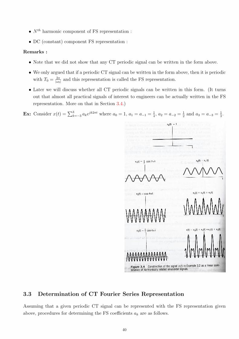
Ex: Consider x(t) =∑3

k=−3 akejk2πt where a0 = 1, a1 = a−1 = 1

4, a2 = a−2 = 1

2and a3 = a−3 = 1

3.

3.3 Determination of CT Fourier Series Representation

Assuming that a given periodic CT signal can be represented with the FS representation given

above, procedures for determining the FS coefficients ak are as follows.

40

3.3.1 Coefficient matching approach

Some signals are inherently expressed as a linear combination of complex exponentials. For such

signals, the FS coefficients ak can be identified by inspection.

Ex: x(t) = sin(ω0t)

Ex: x(t) = 1 + sin(ω0t) + 2 cos(ω0t) + cos(2ω0t+ π4)

3.3.2 General approach

The general approach is given by this integral : ak =1

T0

∫ T0x(t)e−jkω0tdt.

To derive this result, consider a periodic signal with FS representation : x(t) =∑∞

k=−∞ akejkω0t

(fund. period is T0 = 2π|ω0|)

41

Hence, this pair of equations defines the Fourier series of a periodic CT signal :

x(t) =∞∑

k=−∞

akejkω0t ak =

1

T0

∫<T0>

x(t)e−jkω0tdt

Note : The boundaries of the integral can be over an arbitrary interval of one period T0, i.e. from

an arbitrary starting point t0 to t0 +T0, and a typical notation for that is∫<T0>

. The interval should

be chosen according to the signal considered. Typical choices are 0 to T , or −T2

to T2.

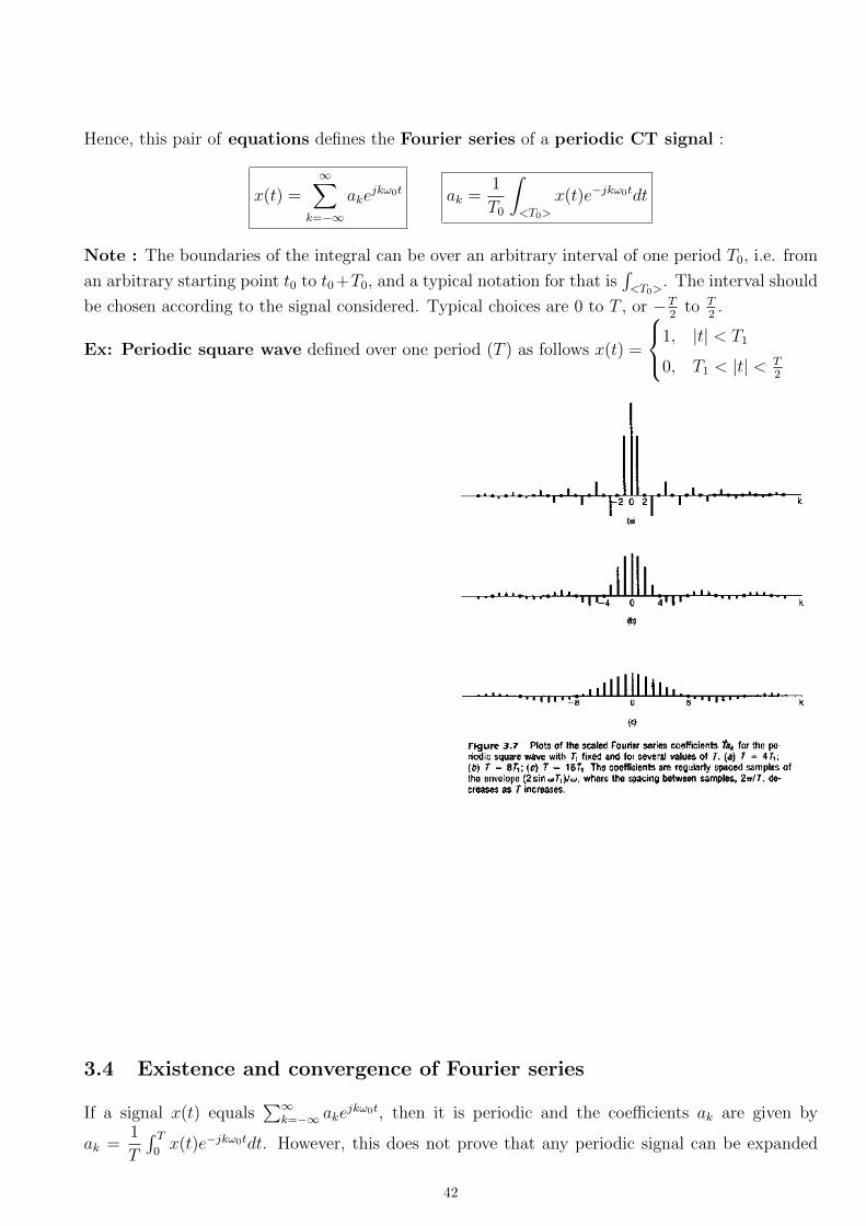
Ex: Periodic square wave defined over one period (T ) as follows x(t) =

1, |t| < T1

0, T1 < |t| < T2

3.4 Existence and convergence of Fourier series

If a signal x(t) equals∑∞

k=−∞ akejkω0t, then it is periodic and the coefficients ak are given by

ak =1

T

∫ T0x(t)e−jkω0tdt. However, this does not prove that any periodic signal can be expanded

42

into∑∞

k=−∞ akejkω0t (i.e. FS representation may not exist.)

In fact, the FS representation exists (i.e. x(t) equals∑∞

k=−∞ akejkω0t) if either

• x(t) has finite energy over one period, i.e.∫T|x(t)|2dt <∞ or

• x(t) satisfies the Dirichlet conditions :

– x(t) is absolutely integrable over any period∫ T

0|x(t)|dt <∞

– x(t) has a finite number of maxima and minima within a period

– x(t) has a finite number of discontinuities within a period.

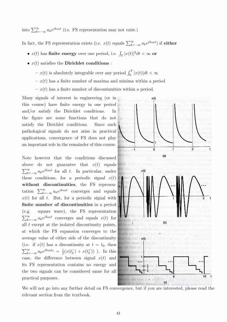
Many signals of interest in engineering (or in

this course) have finite energy in one period

and/or satisfy the Dirichlet conditions. In

the figure are some functions that do not

satisfy the Dirichlet conditions. Since such

pathological signals do not arise in practical

applications, convergence of FS does not play

an important role in the remainder of this course.

Note however that the conditions discussed

above do not guarantee that x(t) equals∑∞k=−∞ ake

jkω0t for all t. In particular, under

these conditions, for a periodic signal x(t)

without discontinuities, the FS represen-

tation∑∞

k=−∞ akejkω0t converges and equals

x(t) for all t. But, for a periodic signal with

finite number of discontinuities in a period

(e.g. square wave), the FS representation∑∞k=−∞ ake

jkω0t converges and equals x(t) for

all t except at the isolated discontinuity points,

at which the FS expansion converges to the

average value of either side of the discontinuity

(i.e. if x(t) has a discontinuity at t = t0, then∑∞k=−∞ ake

jkω0t0 = 12(x(t−0 ) + x(t+0 )) ). In this

case, the difference between signal x(t) and

its FS representation contains no energy and

the two signals can be considered same for all

practical purposes.

We will not go into any further detail on FS convergence, but if you are interested, please read the

relevant section from the textbook.

43

3.5 Properties of Fourier Series

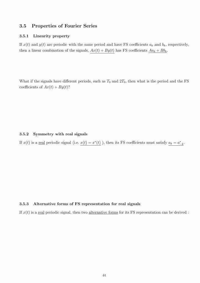
3.5.1 Linearity property

If x(t) and y(t) are periodic with the same period and have FS coefficients ak and bk, respectively,

then a linear combination of the signals, Ax(t) +By(t) has FS coefficients Aak +Bbk.

What if the signals have different periods, such as T0 and 2T0, then what is the period and the FS

coefficients of Ax(t) +By(t)?

3.5.2 Symmetry with real signals

If x(t) is a real periodic signal (i.e. x(t) = x∗(t) ), then its FS coefficients must satisfy ak = a∗−k.

3.5.3 Alternative forms of FS representation for real signals

If x(t) is a real periodic signal, then two alternative forms for its FS representation can be derived :

44

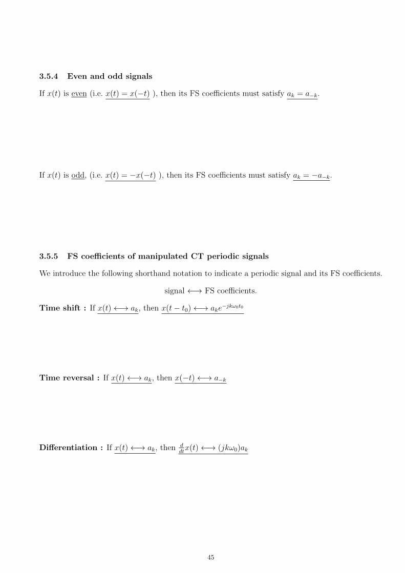
3.5.4 Even and odd signals

If x(t) is even (i.e. x(t) = x(−t) ), then its FS coefficients must satisfy ak = a−k.

If x(t) is odd, (i.e. x(t) = −x(−t) ), then its FS coefficients must satisfy ak = −a−k.

3.5.5 FS coefficients of manipulated CT periodic signals

We introduce the following shorthand notation to indicate a periodic signal and its FS coefficients.

signal ←→ FS coefficients.

Time shift : If x(t)←→ ak, then x(t− t0)←→ ake−jkω0t0

Time reversal : If x(t)←→ ak, then x(−t)←→ a−k

Differentiation : If x(t)←→ ak, then ddtx(t)←→ (jkω0)ak

45

3.5.6 Response of LTI systems to signals with FS representation

In an LTI system, if the input’s FS representation is known, then the output’s FS representation

can be easily obtained from it. (Note that the output will also be periodic with the same period.)

x(t) =∞∑

k=−∞

akejkω0t −→ y(t) =

∞∑k=−∞

akH(jkω0)ejkω0t

Pf:

1. Remember that est is an eigenfunction of LTI systems and the eigenvalue was given by

H(s) =∫∞−∞ e

−sth(t)dt, where s is a general complex number :

2. The system is linear :

Ex: Let input to an LTI system with impulse response h(t) = u(t+ T1

2)− u(t− T1

2) be the periodic

impulse train signal x(t) =∑∞

k=−∞ δ(t − kT ). Find FS coefficients of x(t), and the output y(t).

Also plot y(t). (Assume T > T1.)

Ex: One can find the FS coefficients of a periodic square wave from the FS coefficients of a periodic

impulse train using FS properties. Let us start by finding a relationship between the periodic square

wave and the impulse train signal.

46

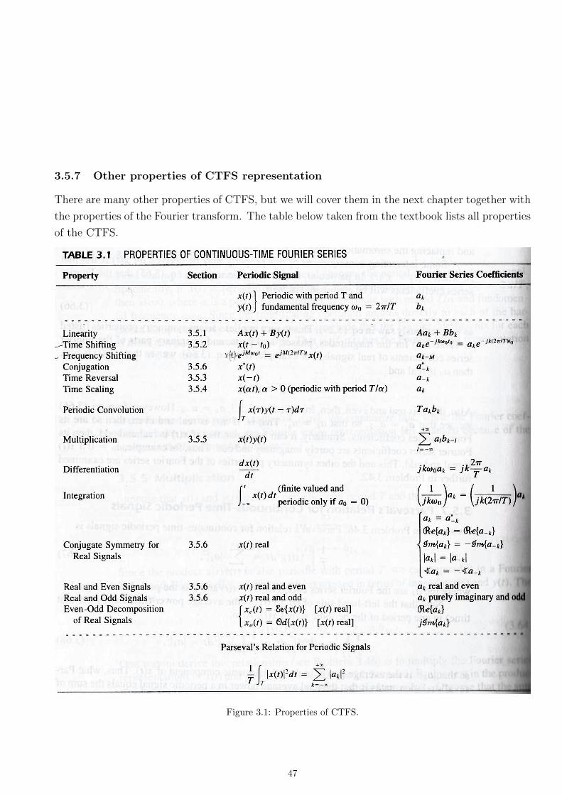
3.5.7 Other properties of CTFS representation

There are many other properties of CTFS, but we will cover them in the next chapter together with

the properties of the Fourier transform. The table below taken from the textbook lists all properties

of the CTFS.

Figure 3.1: Properties of CTFS.

47

Chapter 4

Continuous-time Fourier Transform

Contents

4.1 The Fourier Transform Representation of CT Aperiodic Signals . . . . . . . . . . . . . 49

4.1.1 Intuition behind Fourier transform . . . . . . . . . . . . . . . . . . . . . . . . . . . . . . . . 49

4.1.2 Formal development of Fourier transform . . . . . . . . . . . . . . . . . . . . . . . . . . . . 49

4.2 Convergence of Fourier Transform . . . . . . . . . . . . . . . . . . . . . . . . . . . . . . . 51

4.3 Examples of CT Fourier transforms . . . . . . . . . . . . . . . . . . . . . . . . . . . . . . 51

4.4 Response of LTI systems to complex exponentials (revisited) . . . . . . . . . . . . . . . 53

4.5 Fourier transform of periodic signals . . . . . . . . . . . . . . . . . . . . . . . . . . . . . . 54

4.6 Properties of the Fourier Transform . . . . . . . . . . . . . . . . . . . . . . . . . . . . . . 56

4.6.1 Linearity . . . . . . . . . . . . . . . . . . . . . . . . . . . . . . . . . . . . . . . . . . . . . . 56

4.6.2 Time Shift . . . . . . . . . . . . . . . . . . . . . . . . . . . . . . . . . . . . . . . . . . . . . 56

4.6.3 Time and Frequency Scaling . . . . . . . . . . . . . . . . . . . . . . . . . . . . . . . . . . . 57

4.6.4 Conjugation and Conjugate Symmetry . . . . . . . . . . . . . . . . . . . . . . . . . . . . . . 57

4.6.5 Differentiation and Integration . . . . . . . . . . . . . . . . . . . . . . . . . . . . . . . . . . 59

4.6.6 Duality . . . . . . . . . . . . . . . . . . . . . . . . . . . . . . . . . . . . . . . . . . . . . . . 60

4.6.7 Parseval’s Relation . . . . . . . . . . . . . . . . . . . . . . . . . . . . . . . . . . . . . . . . . 60

4.6.8 Convolution Property . . . . . . . . . . . . . . . . . . . . . . . . . . . . . . . . . . . . . . . 61

4.6.9 Modulation (Multiplication) property . . . . . . . . . . . . . . . . . . . . . . . . . . . . . . 63

4.6.10 Table of properties of CT FT . . . . . . . . . . . . . . . . . . . . . . . . . . . . . . . . . . . 64

4.6.11 Table of basic signals and their CT FT and FS . . . . . . . . . . . . . . . . . . . . . . . . . 65

4.7 Some applications of Fourier transform . . . . . . . . . . . . . . . . . . . . . . . . . . . . 66

4.7.1 Amplitude Modulation (AM) . . . . . . . . . . . . . . . . . . . . . . . . . . . . . . . . . . . 66

4.7.2 Frequency Division Multiplexing (FDM) . . . . . . . . . . . . . . . . . . . . . . . . . . . . . 68

4.7.3 Single Sideband Modulation (SSB) . . . . . . . . . . . . . . . . . . . . . . . . . . . . . . . . 69

In the previous chapter, a representation of CT periodic signals as linear combinations of harmoni-

cally related complex exponentials, i.e. Fourier series, was developed. This representation was also

used to analyze effects of LTI systems on signals with such representation. This chapter extends

these concepts to aperiodic signals.

48

4.1 The Fourier Transform Representation of CT Aperiodic Signals

4.1.1 Intuition behind Fourier transform

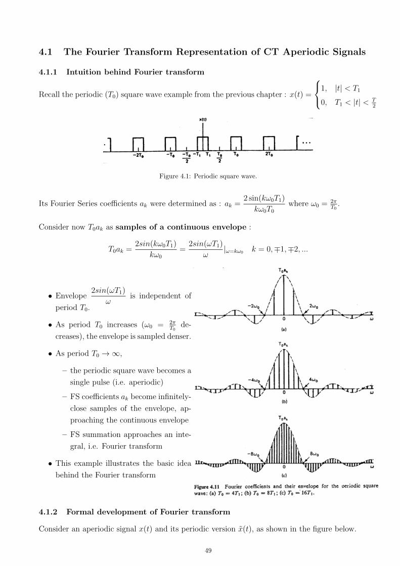
Recall the periodic (T0) square wave example from the previous chapter : x(t) =

1, |t| < T1

0, T1 < |t| < T2

Figure 4.1: Periodic square wave.

Its Fourier Series coefficients ak were determined as : ak =2 sin(kω0T1)

kω0T0

where ω0 = 2πT0

.

Consider now T0ak as samples of a continuous envelope :

T0ak =2sin(kω0T1)

kω0

=2sin(ωT1)

ω|ω=kω0 k = 0,∓1,∓2, ...

• Envelope2sin(ωT1)

ωis independent of

period T0.

• As period T0 increases (ω0 = 2πT0

de-

creases), the envelope is sampled denser.

• As period T0 →∞,

– the periodic square wave becomes a

single pulse (i.e. aperiodic)

– FS coefficients ak become infinitely-

close samples of the envelope, ap-

proaching the continuous envelope

– FS summation approaches an inte-

gral, i.e. Fourier transform

• This example illustrates the basic idea

behind the Fourier transform

4.1.2 Formal development of Fourier transform

Consider an aperiodic signal x(t) and its periodic version x(t), as shown in the figure below.

49

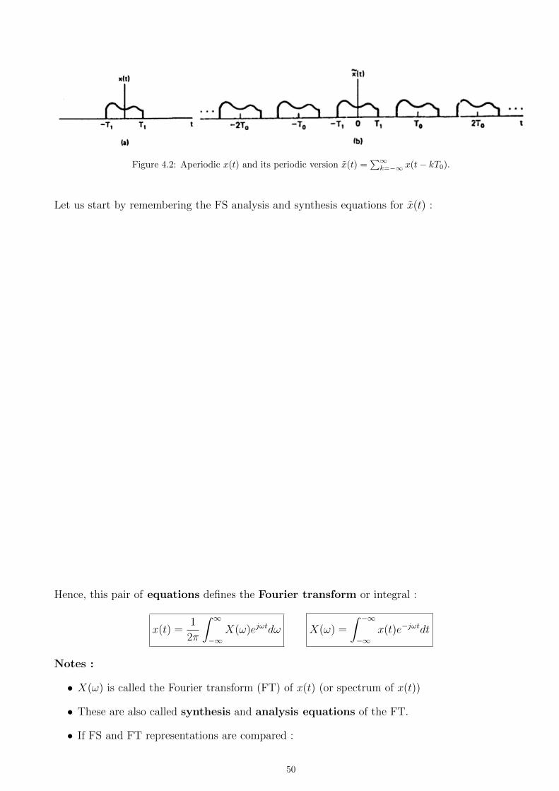
Figure 4.2: Aperiodic x(t) and its periodic version x(t) =∑∞

k=−∞ x(t− kT0).

Let us start by remembering the FS analysis and synthesis equations for x(t) :

Hence, this pair of equations defines the Fourier transform or integral :

x(t) =1

2π

∫ ∞−∞

X(ω)ejωtdω X(ω) =

∫ −∞−∞

x(t)e−jωtdt

Notes :

• X(ω) is called the Fourier transform (FT) of x(t) (or spectrum of x(t))

• These are also called synthesis and analysis equations of the FT.

• If FS and FT representations are compared :

50

– Both represent signals as a linear combination of complex exponentials.

– FS : complex exponentials occur at a discrete set of harmonically related frequencies

kω0 and have amplitudes ak

– FT : complex exponentials occur at a continuum of frequencies and have amplitudesX(ω)

2π– From the development of FT, the FS coefficients ak of x(t) are equally spaced samples of

the FT of x(t) : ak = 1T0X(ω)|ω=kω0

4.2 Convergence of Fourier Transform

Similar to convergence of FS representation, FT representation of a signal x(t) exists (i.e. x(t)

equals1

2π

∫∞−∞X(ω)ejωtdω) if either

• x(t) has finite energy, i.e.∫∞−∞ |x(t)|2dt <∞ or

• x(t) satisfies the Dirichlet conditions :

– x(t) is absolutely integrable , i.e.∫∞−∞ |x(t)|dt <∞

– x(t) has a finite number of maxima and minima within any finite interval

– x(t) has a finite number of discontinuities within any finite interval, and each of these

discontinuities are finite.

Although the above conditions are sufficient to guarantee that a signal has FT, we will see in the

next section that periodic signals, which neither have finite energy nor are absolutely

integrable, can be considered to have FT if impulse functions are permitted in the transform.

This has the advantage that FS and FT representations can be combined into a single framework,

which can be very convenient.

4.3 Examples of CT Fourier transforms

Ex: x(t) = e−atu(t) a > 0.

51

Ex: x(t) = e−a|t| a > 0.

Ex: x(t) = δ(t).

Let us introduce and plot two signals which are convenient to in the following examples and through-

out the course :

1. rect(t) =

1, |t| < 12

0, otherwise

2. sinc(t) =sin(πt)

πt

Ex: Rectangular pulse x(t) =

1, |t| < T1

0, |t| > T1

52

Ex: X(ω) =

1, |ω| < W

0, |ω| > W

Notes :

• rect(t) has FT sinc( ω2π

) and sinc(t) has FT rect( ω2π

)

• A rect() in time domain corresponds to a sinc() in frequency domain and vice versa. (Duality

property of FT)

• As rect() has a shorter (longer) duration, sinc() has a longer (shorter) side lobe. (Scaling prop.

of FT)

4.4 Response of LTI systems to complex exponentials (revisited)

Remember that est is an eigenfunction of LTI systems and the eigenvalue was given by

H(s) =∫∞−∞ e

−sth(t)dt, where s is a general complex number of the form s = α + jω :

Note that if s is purely imaginary (i.e. s = jω), then the complex exponential est = ejωt and its

eigenvalue reduces to the FT of h(t), i.e. we have H(s)|s=jω = Fh(t) = H(ω).

Ex: Let x1(t) = cos(π4t) and x2(t) = cos(3π

4t) be inputs to an LTI system with Fh(t) = H(ω) =

rect(ωπ

). Find outputs y1(t) and y2(t).

53

4.5 Fourier transform of periodic signals

We developed the Fourier transform representation for aperiodic signals. But the FT representation

can also be extended to periodic signals by allowing impulses in the transform X(ω). Hence, the

FT representation can provide a unified framework for representing both periodic and aperiodic

signals, which can be very convenient.

Consider a signal x(t) with Fourier transform X(ω) that is a single impulse of strength 2π at ω = ω0:

More generally, consider a linear combination of impulses equally spaced in frequency :

In summary, to determine the FT of a periodic signal,

1. determine its FS coefficients ak

2. then write its FT as X(ω) =∑∞

k=−∞ 2πakδ(ω − kω0).

Ex: x(t) = cos(ω0t)

54

Ex: x(t) = sin(ω0t)

Ex: The periodic square wave (again!)

Ex: Periodic impulse train x(t) =∑∞

k=−∞ δ(t− kT )

55

4.6 Properties of the Fourier Transform

To discuss Fourier transform properties, it is convenient to use the following shorthand notation to

indicate the pairing of a signal and its transform :

• signal ←→ FT ( e.g. x(t)←→ X(ω) )

We sometimes also refer to a FT and inverse FT with the following notation :

• Fsignal and F−1FT ( e.g. X(ω) = Fx(t) and x(t) = F−1X(ω))

For the following properties, let us assume that we have two signals x(t) and y(t) with corresponding

FT X(ω) and Y (ω), i.e.

x(t)←→ X(ω) and y(t)←→ Y (ω).

We will also discuss some FS properties along with the corresponding FT properties since we omitted

many FS properties in the previous chapter. Hence, we will use the same notation to indicate the

pairing of a periodic signal and its FS coefficients. We will also use a tilde on top of periodic signals

to differentiate them from aperiodic signals. To discuss FS properties, let us again assume that

we have two periodic signals x(t) and y(t) with the same period T0 and have corresponding FS

coefficients ak and bk, i.e.

x(t)←→ ak and y(t)←→ bk.

4.6.1 Linearity

ax(t) + by(t)←→ aX(ω) + bY (ω)

(FS: Ax(t) +By(t)←→ Aak +Bbk What if x(t) and y(t) do not have the same period ?)

4.6.2 Time Shift

x(t− t0)←→ e−jωt0X(ω)

(FS: x(t− t0)←→ e−jkω0t0ak )

56

4.6.3 Time and Frequency Scaling

x(at)←→ 1

|a|X(

ω

a)

Note that this property indicates that time and frequency parameters scale inversely proportional.

When one expands, the other contracts.

(FS: x(at) becomes periodic with and x(at)←→ ak )

Let us write down and compare the FS expansions of x(t) and x(at):

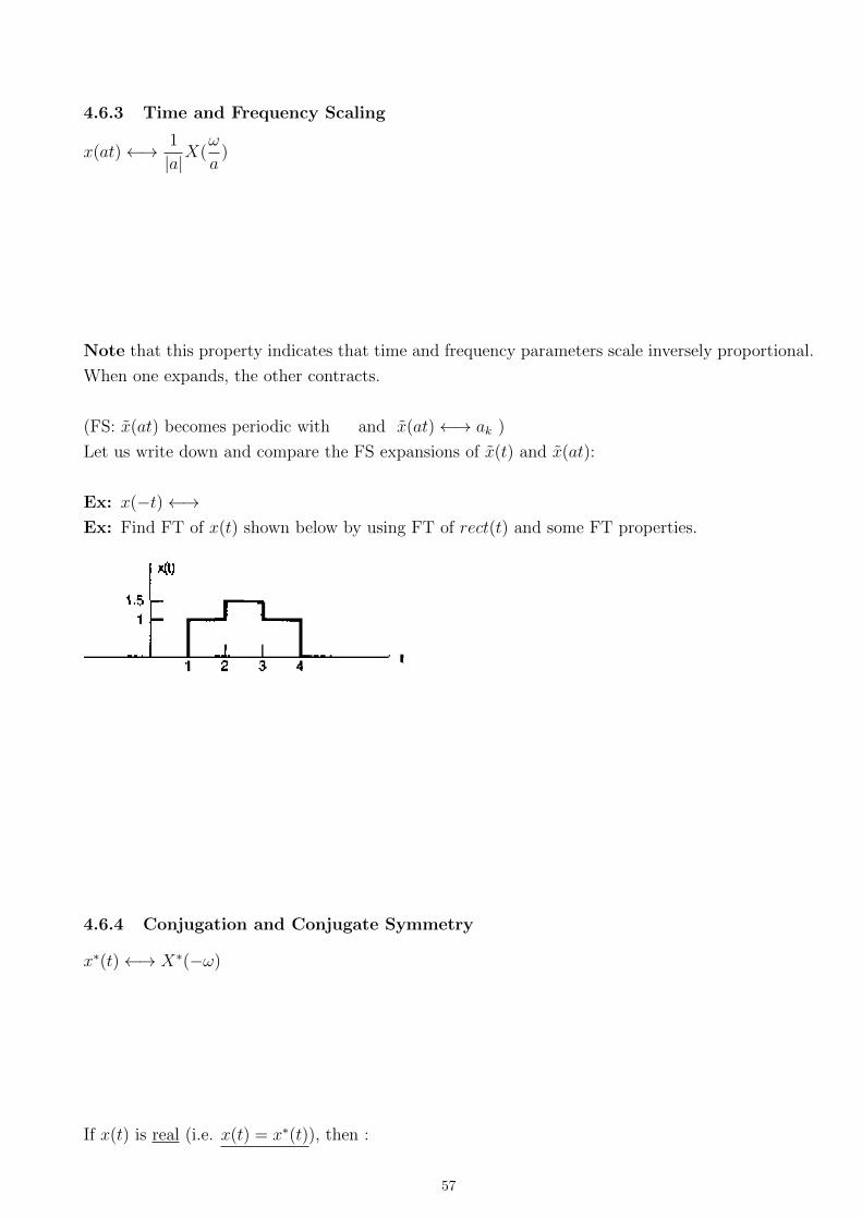
Ex: x(−t)←→Ex: Find FT of x(t) shown below by using FT of rect(t) and some FT properties.

4.6.4 Conjugation and Conjugate Symmetry

x∗(t)←→ X∗(−ω)

If x(t) is real (i.e. x(t) = x∗(t)), then :

57

• X(ω) = or X∗(ω) =

• ReX(ω) = ReX(−ω) and ImX(ω) = −ImX(−ω)

• |X(ω)| = |X(−ω)| and ∠X(ω) = −∠X(−ω)

If x(t) is both real and even (i.e. x(t) = x∗(t) = x(−t)), then

• X(ω) is also both real and even.

If x(t) is both real and odd (i.e. x(t) = x∗(t) = −x(−t)), then

• X(ω) is purely imaginary and odd.

Remember that any real signal x(t) can be uniquely written as a sum of its even and odd parts:

x(t) = xe(t) + xo(t). Using some of the above properties it can be shown that :

• xe(t)←→ ReX(ω)

• xo(t)←→ j · ImX(ω)

Showing these properties is left as an exercise.

(FS : x∗(t) ←→ a∗−k ) Similar properties exist in case x(t) is real, real and even, etc. See the

CTFS properties table in the previous chapter in Section 3.5.7

Ex: x(t) = e−|a|t , a > 0.

58

4.6.5 Differentiation and Integration

d

dtx(t)←→ jω ·X(ω) and

∫ t−∞ x(τ)dτ ←→ 1

jωX(ω) + πX(0)δ(ω)

(FS:d

dtx(t)←→ jkω0 · ak and

∫ t=∞ x(τ)dτ ←→ 1

jkω0

ak)

Note that∫ t

=∞ x(τ)dτ is finite and periodic only if a0 = 0.

Ex: Find impulse response of LTI system described by ddty(t) + αy(t) = x(t)

Ex: Find FT of linear ramp signal

Ex: Find FT of unit step signal u(t)

59

4.6.6 Duality

X(t)←→ 2πx(−ω) ( Or alternatively if g(t)←→ f(ω) then, f(t)←→ 2πg(−ω))

Ex: x(t) =1

1 + t2

Ex: Rectangular pulse and sinc functions. rect(t)←→ sinc( ω2π

) implies

Duality principle can be applied to derive additional properties :

• Frequency shift :

• Frequency differentiation :

• Frequency integration :

4.6.7 Parseval’s Relation∫ ∞−∞|x(t)|2dt =

1

2π

∫ ∞−∞|X(ω)|2dω

• The term on left side is the total energy in the signal x(t).

• Parseval’s relation indicates that the total signal energy can be computed either

– from x(t) by integrating its energy per unit time (|x(t)|2) over all time

– or from X(ω) by integrating its energy per unit frequency (|X(ω)|2

2π) over all frequencies.

• |X(ω)|2 is called the energy-density spectrum of signal x(t).

60

(FS:1

T0

∫T0

|x(t)|2dt =∞∑

k=−∞

|ak|2 Left side of equation is the average power of the periodic

signal x(t), and equals to the sum of squared magnitudes of FS coefficients.)

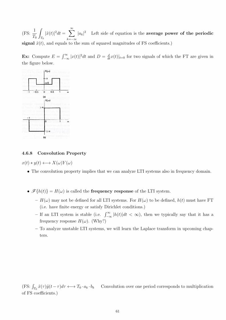
Ex: Compute E =∫∞−∞ |x(t)|2dt and D = d

dtx(t)|t=0 for two signals of which the FT are given in

the figure below.

4.6.8 Convolution Property

x(t) ∗ y(t)←→ X(ω)Y (ω)

• The convolution property implies that we can analyze LTI systems also in frequency domain.

• Fh(t) = H(ω) is called the frequency response of the LTI system.

– H(ω) may not be defined for all LTI systems. For H(ω) to be defined, h(t) must have FT

(i.e. have finite energy or satisfy Dirichlet conditions.)

– If an LTI system is stable (i.e.∫∞−∞ |h(t)|dt < ∞), then we typically say that it has a

frequency response H(ω). (Why?)

– To analyze unstable LTI systems, we will learn the Laplace transform in upcoming chap-

ters.

(FS:∫T0x(τ)y(t− τ)dτ ←→ T0 ·ak · bk Convolution over one period corresponds to multiplication

of FS coefficients.)

61

Ex: An LTI system with h(t) = δ(t − t0). Find its frequency response H(ω) and the outputs FT

in terms of the input’s FT.

Ex: The differentiator is an LTI system. Find its frequency response.

Ex: Consider an LTI system with h(t) = e−atu(t) and an input x(t) = e−btu(t) where a > 0 and

b > 0. While the output can be computed in time domain via convolution, let us find the output

in frequency domain first and then in time-domain.

Ex: Frequency selective filtering is accomplished with an LTI system whose frequency response

H(ω) passes desired range of frequencies and significantly attenuates frequencies outside that range.

Consider the ideal low-pass filter with H(ω) =

1, |ω| < ωc

0, otherwise.

62

Ex: Consider an ideal LPF with cut-off frequency wc and an input signal x(t) =sin(ωit)

πt. Calculate

the output.

4.6.9 Modulation (Multiplication) property

x(t) · y(t)←→ 1

2πX(ω) ∗ Y (ω)

• Multiplication of one signal by another can be thought of using one signal to scale or modulate

the amplitude of the other.

• Considering also the convolution property, it can be stated that convolution in one domain

corresponds to multiplication in the other domain (Duality property.)

(FS: x(t) · y(t)←→ ak ∗ bk =∑∞

l=−∞ albk−l)

Ex: x(t) = m(t)ejω0t. Find X(ω) in terms of spectrum of m(t).

Ex: Let signal s(t) have spectrum S(ω) as below and also consider signal p(t) = cos(ω0t). Determine

the spectrum of r(t) = s(t) · p(t).

63

Ex: Find FT of x(t) =sin(t) sin( t

2)

πt2.

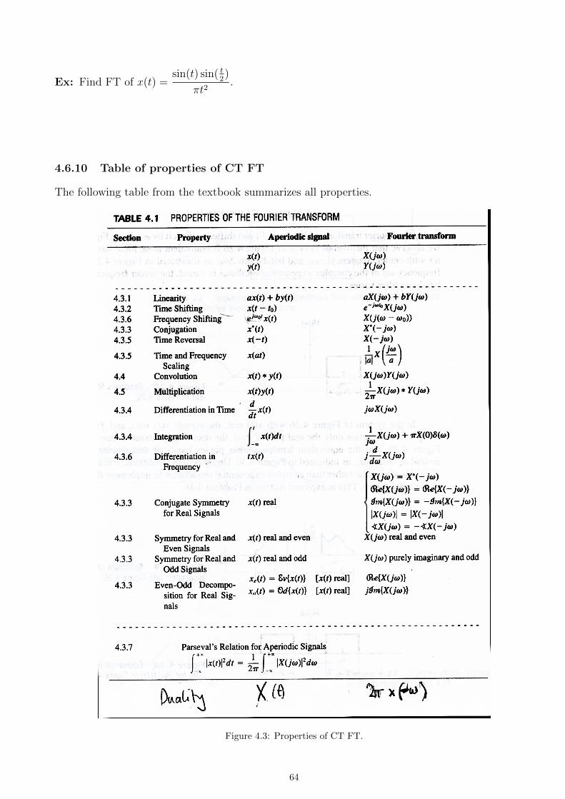
4.6.10 Table of properties of CT FT

The following table from the textbook summarizes all properties.

Figure 4.3: Properties of CT FT.

64

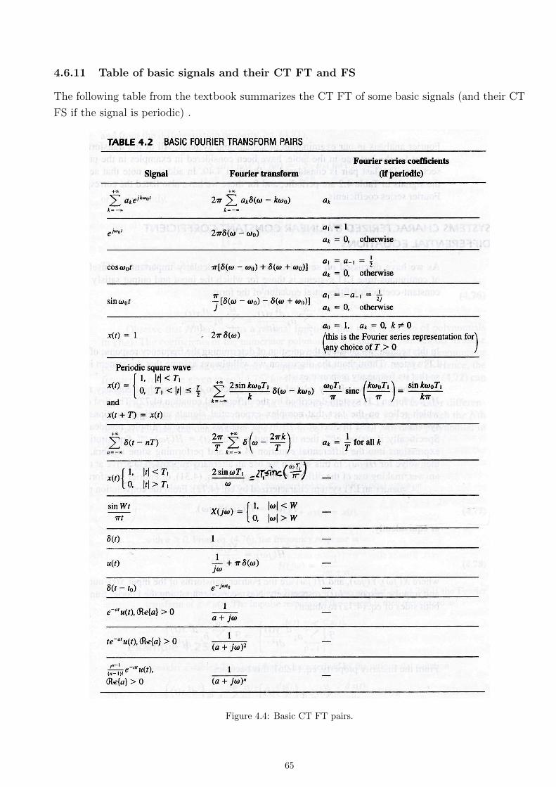
4.6.11 Table of basic signals and their CT FT and FS

The following table from the textbook summarizes the CT FT of some basic signals (and their CT

FS if the signal is periodic) .

Figure 4.4: Basic CT FT pairs.

65

4.7 Some applications of Fourier transform

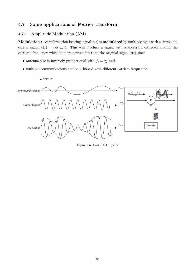
4.7.1 Amplitude Modulation (AM)

Modulation : An information bearing signal x(t) is modulated by multiplying it with a sinusoidal

carrier signal c(t) = cos(ωct). This will produce a signal with a spectrum centered around the

carrier’s frequency which is more convenient than the original signal x(t) since

• antenna size is inversely proportional with fc = ωc2π

and

• multiple communications can be achieved with different carriers frequencies.

Figure 4.5: Basic CTFT pairs.

66

Demodulation : Recovery of the original information bearing signal x(t) from the modulated

signal. We will discuss synchronous demodulation, where the frequency and phase of the carrier

is assumed to be known perfectly at the receiver.

Synchronous demodulation is achieved in two steps :

1. modulate with the same carrier and

2. low-pass filter

In summary,

• Modulation :

• Demodulation :

67

4.7.2 Frequency Division Multiplexing (FDM)

If multiple information bearing signals need to be transmitted at the same time, each can be

modulated to different carrier frequencies.

How about demodulation in FDM ?

68

4.7.3 Single Sideband Modulation (SSB)

Consider a real signal x(t).

69

Chapter 5

Discrete-time Fourier Series and

Transform

Contents

5.1 DT Fourier Series . . . . . . . . . . . . . . . . . . . . . . . . . . . . . . . . . . . . . . . . . 71

5.1.1 Response of DT LTI Systems to Complex Exponentials . . . . . . . . . . . . . . . . . . . . 71

5.1.2 DT Fourier series representation of periodic DT signals . . . . . . . . . . . . . . . . . . . . 72

5.2 DT Fourier Transform . . . . . . . . . . . . . . . . . . . . . . . . . . . . . . . . . . . . . . 75

5.2.1 Intuition and formal development of DT Fourier transform . . . . . . . . . . . . . . . . . . 75

5.2.2 Convergence of DT Fourier transform . . . . . . . . . . . . . . . . . . . . . . . . . . . . . . 76

5.2.3 Examples of DT Fourier transform . . . . . . . . . . . . . . . . . . . . . . . . . . . . . . . . 76

5.2.4 Response of LTI systems to complex exponentials (revisited) . . . . . . . . . . . . . . . . . 77

5.2.5 DT Fourier transform of periodic signals . . . . . . . . . . . . . . . . . . . . . . . . . . . . . 78

5.3 Properties of DT Fourier series and transform . . . . . . . . . . . . . . . . . . . . . . . . 80

5.3.1 Periodicity . . . . . . . . . . . . . . . . . . . . . . . . . . . . . . . . . . . . . . . . . . . . . 80

5.3.2 Linearity . . . . . . . . . . . . . . . . . . . . . . . . . . . . . . . . . . . . . . . . . . . . . . 80

5.3.3 Time Shifting and Frequency Shifting . . . . . . . . . . . . . . . . . . . . . . . . . . . . . . 80

5.3.4 Conjugation and Conjugate Symmetry . . . . . . . . . . . . . . . . . . . . . . . . . . . . . . 81

5.3.5 Differencing and Accumulation . . . . . . . . . . . . . . . . . . . . . . . . . . . . . . . . . . 82

5.3.6 Time Reversal . . . . . . . . . . . . . . . . . . . . . . . . . . . . . . . . . . . . . . . . . . . 82

5.3.7 Differentiation in Frequency . . . . . . . . . . . . . . . . . . . . . . . . . . . . . . . . . . . . 82

5.3.8 Time Expansion . . . . . . . . . . . . . . . . . . . . . . . . . . . . . . . . . . . . . . . . . . 82

5.3.9 Parseval’s Relation . . . . . . . . . . . . . . . . . . . . . . . . . . . . . . . . . . . . . . . . . 84

5.3.10 Convolution Property . . . . . . . . . . . . . . . . . . . . . . . . . . . . . . . . . . . . . . . 85

5.3.11 Multiplication property . . . . . . . . . . . . . . . . . . . . . . . . . . . . . . . . . . . . . . 86

5.3.12 Table of properties of DT FT and FS . . . . . . . . . . . . . . . . . . . . . . . . . . . . . . 87

5.3.13 Table of basic signals and their DT FT and FS . . . . . . . . . . . . . . . . . . . . . . . . . 87

This chapter discusses Fourier series and transform representations for discrete-time signals. Similar

to the CT representations, the DT Fourier series represents DT periodic signals as a linear combina-

tion of harmonically related DT complex exponentials and the DT Fourier transform representation

extends this approach to aperiodic DT signals.

70

5.1 DT Fourier Series

5.1.1 Response of DT LTI Systems to Complex Exponentials

Similar to the CT case, DT complex exponentials x[n] = zn = (rejΩ0)n are eigenfunctions of DT

LTI systems.

Again, representation of DT signals as a linear combination of DT complex exponentials is very

useful since

• such a representation can form a broad and useful class of signals and

• the response of the LTI system to a signal with such representation is easily determined:

Ex: Let an LTI system have impulse response h[n] = 12δ[n+ 1] + δ[n] + 1

2δ[n− 1]. Find outputs of

system for inputs x1[n] = cos(π2n) and x2[n] = sin(πn).

71

5.1.2 DT Fourier series representation of periodic DT signals

Remember that for CT complex exponentials,

• x(t) = ejω0t is always periodic with period T0 = 2π|ω0|

• the set of all complex exponentials that have a common period T0 = 2π|ω0| are given by

φk(t) = ejk 2πT0t, k = 0,±1,±2, ...

For DT complex exponentials,

• x[n] = ejΩ0n is periodic only if Ω0 is in the form

• the period of x[n] = ej2πNn is N

• the set of all complex exponentials that have a common period N are given by

φk[n] = ejk2πNn, k = 0,±1,±2, ...

Another important difference between CT and DT complex exponentials is that while

• ejkω0t are always distinct for different k,

• there are only N distinct ejk2πNn, in particular, ejk

2πNn = ej(k+rN) 2π

Nn where r ∈ Z

Hence, a linear combination of DT complex exponentials of the form∑k

akejk 2π

Nn

• is periodic with N

• and the summation needs to go over only N successive values of k.

Let us now introduce the DT Fourier series representation :

x[n] =

k0+N−1∑k=k0

akejk 2π

Nn.

• A representation of this form is called the Fourier series representation of periodic DT signal

x[n] with fundamental period N .

72

• Coefficients ak are called the Fourier series (FS) coefficients (or spectral coefficients).

• Fundamental, N th harmonic, and DC (constant) components of the FS representation are

defined in the same way as in the CT FS representation.

• Note that the summation goes over N consecutive values of k starting at an arbitrary value

k0, which is commonly shown with the notation∑

k=<N>.

Existence of DT FS

Unlike the existence of CT FS, the existence of DT FS is worry-free. The DT FS representation

always exist for any finite periodic DT signal x[n].

To see this, consider the set of N linearly independent equations for coefficients ak obtainable from

the DT FS representation :

x[0] =

k0+N−1∑k=k0

ak

x[1] =

k0+N−1∑k=k0

akejk 2π

N

......

x[N − 1] =

k0+N−1∑k=k0

akejk 2π

N(N−1)

It can be shown that these N equations are linearly independent (see Problem 3.32 in textbook)

and thus FS coefficients ak exist uniquely.

Determination of DT Fourier series representation

For a given DT periodic sequence x[n], one way to determine the DT FS coefficients ak, is to solve

the above set of linear equations. However, similar to the CT FS, it is also possible to obtain a

closed form solution for the coefficients ak :

73

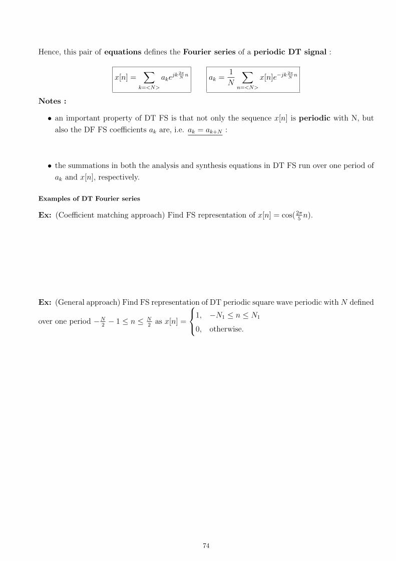
Hence, this pair of equations defines the Fourier series of a periodic DT signal :

x[n] =∑

k=<N>

akejk 2π

Nn ak =

1

N

∑n=<N>

x[n]e−jk2πNn

Notes :

• an important property of DT FS is that not only the sequence x[n] is periodic with N, but

also the DF FS coefficients ak are, i.e. ak = ak+N :

• the summations in both the analysis and synthesis equations in DT FS run over one period of

ak and x[n], respectively.

Examples of DT Fourier series

Ex: (Coefficient matching approach) Find FS representation of x[n] = cos(2π5n).

Ex: (General approach) Find FS representation of DT periodic square wave periodic with N defined

over one period −N2− 1 ≤ n ≤ N

2as x[n] =

1, −N1 ≤ n ≤ N1

0, otherwise.

74

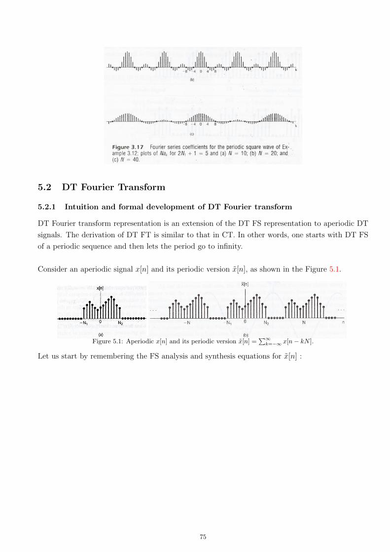
5.2 DT Fourier Transform

5.2.1 Intuition and formal development of DT Fourier transform

DT Fourier transform representation is an extension of the DT FS representation to aperiodic DT

signals. The derivation of DT FT is similar to that in CT. In other words, one starts with DT FS

of a periodic sequence and then lets the period go to infinity.

Consider an aperiodic signal x[n] and its periodic version x[n], as shown in the Figure 5.1.

Figure 5.1: Aperiodic x[n] and its periodic version x[n] =∑∞

k=−∞ x[n− kN ].

Let us start by remembering the FS analysis and synthesis equations for x[n] :

75

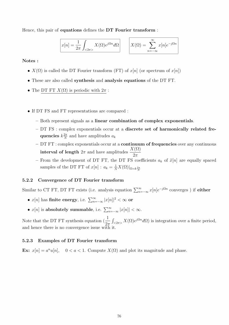
Hence, this pair of equations defines the DT Fourier transform :

x[n] =1

2π

∫<2π>

X(Ω)ejΩndΩ X(Ω) =∞∑

n=−∞

x[n]e−jΩn

Notes :

• X(Ω) is called the DT Fourier transform (FT) of x[n] (or spectrum of x[n])

• These are also called synthesis and analysis equations of the DT FT.

• The DT FT X(Ω) is periodic with 2π :

• If DT FS and FT representations are compared :

– Both represent signals as a linear combination of complex exponentials.

– DT FS : complex exponentials occur at a discrete set of harmonically related fre-

quencies k 2πN

and have amplitudes ak

– DT FT : complex exponentials occur at a continuum of frequencies over any continuous

interval of length 2π and have amplitudesX(Ω)

2π– From the development of DT FT, the DT FS coefficients ak of x[n] are equally spaced

samples of the DT FT of x[n] : ak = 1NX(Ω)|Ω=k 2π

N

5.2.2 Convergence of DT Fourier transform

Similar to CT FT, DT FT exists (i.e. analysis equation∑∞

n=−∞ x[n]e−jΩn converges ) if either

• x[n] has finite energy, i.e.∑∞

n=−∞ |x[n]|2 <∞ or

• x[n] is absolutely summable, i.e.∑∞

n=−∞ |x[n]| <∞.

Note that the DT FT synthesis equation (1

2π

∫<2π>

X(Ω)ejΩndΩ) is integration over a finite period,

and hence there is no convergence issue with it.

5.2.3 Examples of DT Fourier transform

Ex: x[n] = anu[n], 0 < a < 1. Compute X(Ω) and plot its magnitude and phase.

76

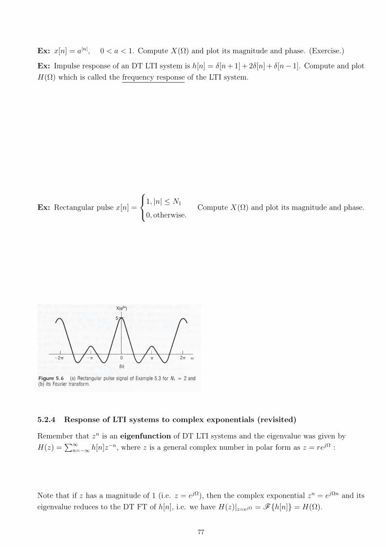
Ex: x[n] = a|n|, 0 < a < 1. Compute X(Ω) and plot its magnitude and phase. (Exercise.)

Ex: Impulse response of an DT LTI system is h[n] = δ[n+ 1] + 2δ[n] + δ[n− 1]. Compute and plot

H(Ω) which is called the frequency response of the LTI system.

Ex: Rectangular pulse x[n] =

1, |n| ≤ N1

0, otherwise.Compute X(Ω) and plot its magnitude and phase.

5.2.4 Response of LTI systems to complex exponentials (revisited)

Remember that zn is an eigenfunction of DT LTI systems and the eigenvalue was given by

H(z) =∑∞

n=−∞ h[n]z−n, where z is a general complex number in polar form as z = rejΩ :

Note that if z has a magnitude of 1 (i.e. z = ejΩ), then the complex exponential zn = ejΩn and its

eigenvalue reduces to the DT FT of h[n], i.e. we have H(z)|z=ejΩ = Fh[n] = H(Ω).

77

Ex: Let x1[n] = cos(π4n) and x2[n] = cos(3π

4n) be inputs to an LTI system with Fh[n] = H(Ω) =

rect(Ωπ

) , |Ω| < π2

and 0 otherwise in |Ω| < π. Find outputs y1[n] and y2[n].

5.2.5 DT Fourier transform of periodic signals

As in the CT case, periodic DT signals can also be represented with the DT FT by allowing impulses

in the transform. Hence, as in CT, the DT FT can serve as a common framework for representing

both periodic and aperiodic DT signals.

Let us start with the result : the expression for the DT FT of a periodic DT signal x[n] is very

similar to the expression we obtained previously for the CT FT of a periodic CT signal x(t).

Remember, in CT, we could obtain the CT FT of a periodic signal x(t) with FS coefficients ak and

fundamental frequency ω0 via an impulse train :

x(t) =∞∑

k=−∞

akejkω0t ←→ X(ω) =

∞∑k=−∞

2πakδ(ω − kω0)

In DT, the DT FT of a periodic sequence x[n] with periodic DT FS coefficients ak and fundamental

frequency Ω0 =2π

Ncan be obtained via a very similar impulse train :

x[n] =∑

k=<N>

akejk 2π

Nn ←→ X(Ω) =

∞∑k=−∞

2πakδ(Ω− kΩ0) where Ω0 =2π

N.

Let us derive this expression, by first considering the DT FT of ejΩ0n :

• In CT, remember that the FT of ejω0t was : ejω0t ←→ 2πδ(ω − ω0)

• In DT, the FT must be periodic with 2π, so let us try for the DT FT of ejΩ0n a periodic

impulse train

ejΩ0n ←→∞∑l=∞

2πδ(Ω− Ω0 − 2πl)

78

Now, consider the DT FS of a periodic DT signals x[n] and use the above result :

In summary, to determine the DT FT of a periodic signal, (as we did in CT)

1. determine its periodic DT FS coefficients ak

2. then write its DT FT as X(Ω) =∑∞

k=−∞ 2πakδ(Ω− kΩ0) where Ω0 = 2πN

.

Ex: cos(2π5n). Find its DT FT.

Ex: Find DT FT of DT periodic impulse train x[n] =∑∞

k=−∞ δ[n− kN ].

79

5.3 Properties of DT Fourier series and transform

To discuss the DT Fourier transform and series properties, we use the same convenient shorthand

notation we used in CT FS and FT properties. In other words, to indicate the pairing of a signal

and its transform, we use :

• signal ←→ FT ( e.g. x[n]←→ X(Ω) )

We sometimes also refer to a FT and inverse FT with the following notation :

• Fsignal and F−1FT ( e.g. X(Ω) = Fx[n] and x[n] = F−1X(Ω))

For the following properties, let us assume that we have two signals x[n] and y[n] with corresponding

DT FT X(Ω) and Y (Ω), i.e.

x[n]←→ X(Ω) and y[n]←→ Y (Ω).

Let us also assume we have two periodic signals x[n] and y[n], periodic with the same period N ,

with corresponding DT FS coefficients ak and bk, i.e.

x[n]←→ ak and y[n]←→ bk.

5.3.1 Periodicity

X(Ω) = X(Ω + 2π)

(FS: ak = ak+N)

5.3.2 Linearity

ax[n] + by[n]←→ aX(Ω) + bY (Ω)

(FS: Ax[n] +By[n]←→ Aak +Bbk What if x[n] and y[n] do not have the same period ?)

5.3.3 Time Shifting and Frequency Shifting

x[n− n0]←→ e−jΩn0X(Ω) and ejΩ0nx[n]←→ X(Ω− Ω0)

80

(FS: x[n− n0]←→ e−jk2πNn0ak and ejk0

2πNnx[n]←→ ak−k0 )

Ex: Consider the frequency response HILP (Ω) of the ideal DT low-pass filter with cut-off frequency

Ωc, plotted below. Plot and discuss HIHP (Ω) = HILP (Ω − π). Also obtain hIHP [n] in terms of

hILP [n].

5.3.4 Conjugation and Conjugate Symmetry

x∗[n]←→ X∗(−Ω)

Properties similar to the CT case can be obtained if x[n] is real (i.e. x[n] = x∗[n]) :

• X(Ω) = or X∗(Ω) =

• ReX(Ω) = ReX(−Ω) and ImX(Ω) = −ImX(−Ω)

• |X(Ω)| = |X(−Ω)| and ∠X(Ω) = −∠X(−Ω)

Similar to the CT case, again,

• if x[n] is both real and even (i.e. x[n] = x∗[n] = x[−n]), then X(Ω) is also both real and even

• if x[n] is both real and odd (i.e. x[n] = x∗[n] = −x[−n]), thenX(Ω) is purely imaginary and odd.

(FS : x∗[n]←→ a∗−k ) Similar properties exist in case x[n] is real, real and even, etc.

For a summary of all conjugate symmetry properties of DT FT and FS, see the properties tables

in the upcoming Section 5.3.12.

81

5.3.5 Differencing and Accumulation

x[n]− x[n− 1]←→ (1− ejΩ)X(Ω) andn∑

m=−∞

x[m]←→ 1

1− ejΩX(Ω) + πX(0)

∞∑k=−∞

δ(Ω− 2πk)

(FS: x[n]− x[n− 1]←→ (1− ejk 2πN )ak and

∑nm=−∞ x[m]←→ 1

1− ejk 2πN

ak )

Note that∑n

m=−∞ x[m] is finite and period only if a0 = 0.

Ex: Find Fu[n].

5.3.6 Time Reversal

x[−n]←→ X(−Ω)

(FS: x[−n]←→ a−k)

5.3.7 Differentiation in Frequency

nx[n]←→ jd

dΩX(Ω)

5.3.8 Time Expansion

Remember the CT FT result for time expansion (scaling) : x(at)←→ 1

|a|X(

ω

a).

If we try to define similarly the signal x[an], we run into difficulties if a is not an integer.

In CT, if a > 1, then this speeds up the signal (i.e. compresses signal wrt origin.) Let’s similarly,

consider x[an] for an integer a such that a > 1. This not only speeds up the signal but also discards

some samples of x[n] :

82

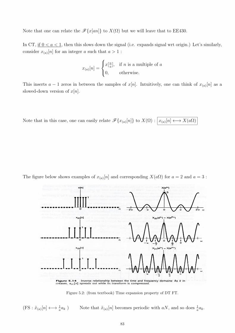
Note that one can relate the Fx[an] to X(Ω) but we will leave that to EE430.

In CT, if 0 < a < 1, then this slows down the signal (i.e. expands signal wrt origin.) Let’s similarly,

consider x(a)[n] for an integer a such that a > 1 :

x(a)[n] =

x[na], if n is a multiple of a

0, otherwise.

This inserts a − 1 zeros in between the samples of x[n]. Intuitively, one can think of x(a)[n] as a

slowed-down version of x[n].

Note that in this case, one can easily relate Fx(a)[n] to X(Ω) : x(a)[n]←→ X(aΩ)

The figure below shows examples of x(a)[n] and corresponding X(aΩ) for a = 2 and a = 3 :

Figure 5.2: (from textbook) Time expansion property of DT FT.

(FS : x(a)[n]←→ 1aak ) Note that x(a)[n] becomes periodic with aN , and so does 1

aak.

83

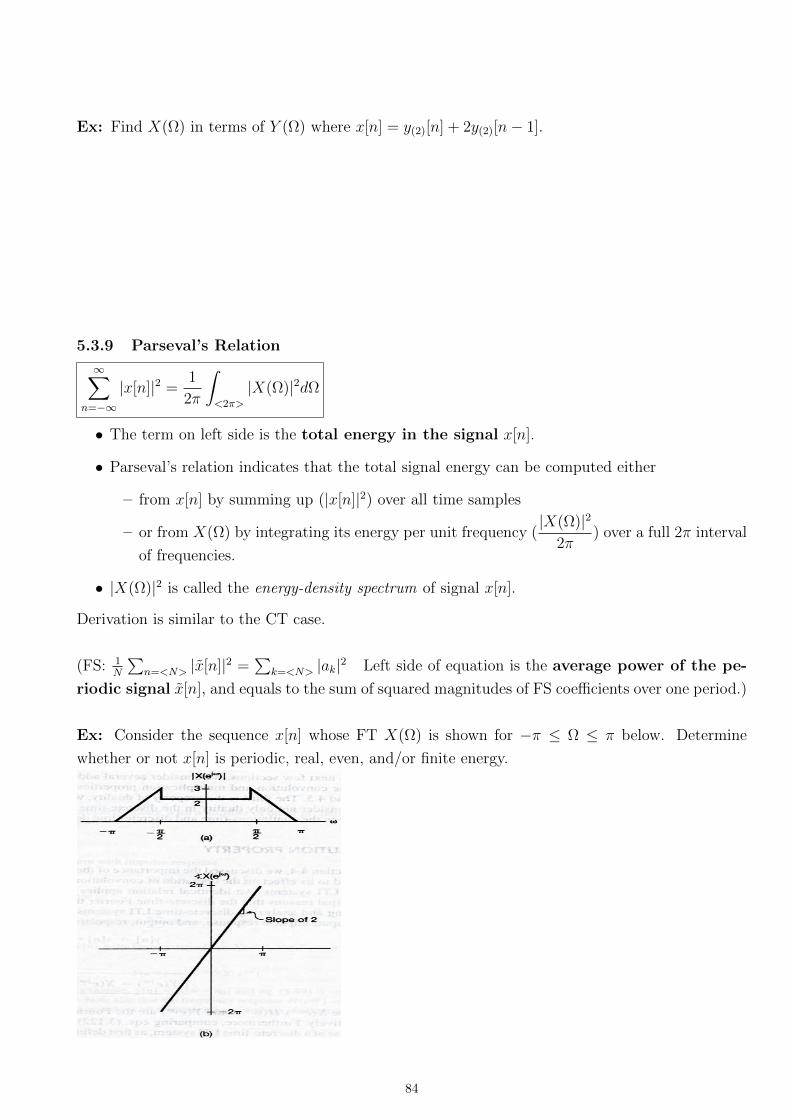
Ex: Find X(Ω) in terms of Y (Ω) where x[n] = y(2)[n] + 2y(2)[n− 1].

5.3.9 Parseval’s Relation

∞∑n=−∞

|x[n]|2 =1

2π

∫<2π>

|X(Ω)|2dΩ

• The term on left side is the total energy in the signal x[n].

• Parseval’s relation indicates that the total signal energy can be computed either

– from x[n] by summing up (|x[n]|2) over all time samples

– or from X(Ω) by integrating its energy per unit frequency (|X(Ω)|2

2π) over a full 2π interval

of frequencies.

• |X(Ω)|2 is called the energy-density spectrum of signal x[n].

Derivation is similar to the CT case.

(FS: 1N

∑n=<N> |x[n]|2 =

∑k=<N> |ak|2 Left side of equation is the average power of the pe-

riodic signal x[n], and equals to the sum of squared magnitudes of FS coefficients over one period.)

Ex: Consider the sequence x[n] whose FT X(Ω) is shown for −π ≤ Ω ≤ π below. Determine

whether or not x[n] is periodic, real, even, and/or finite energy.

84

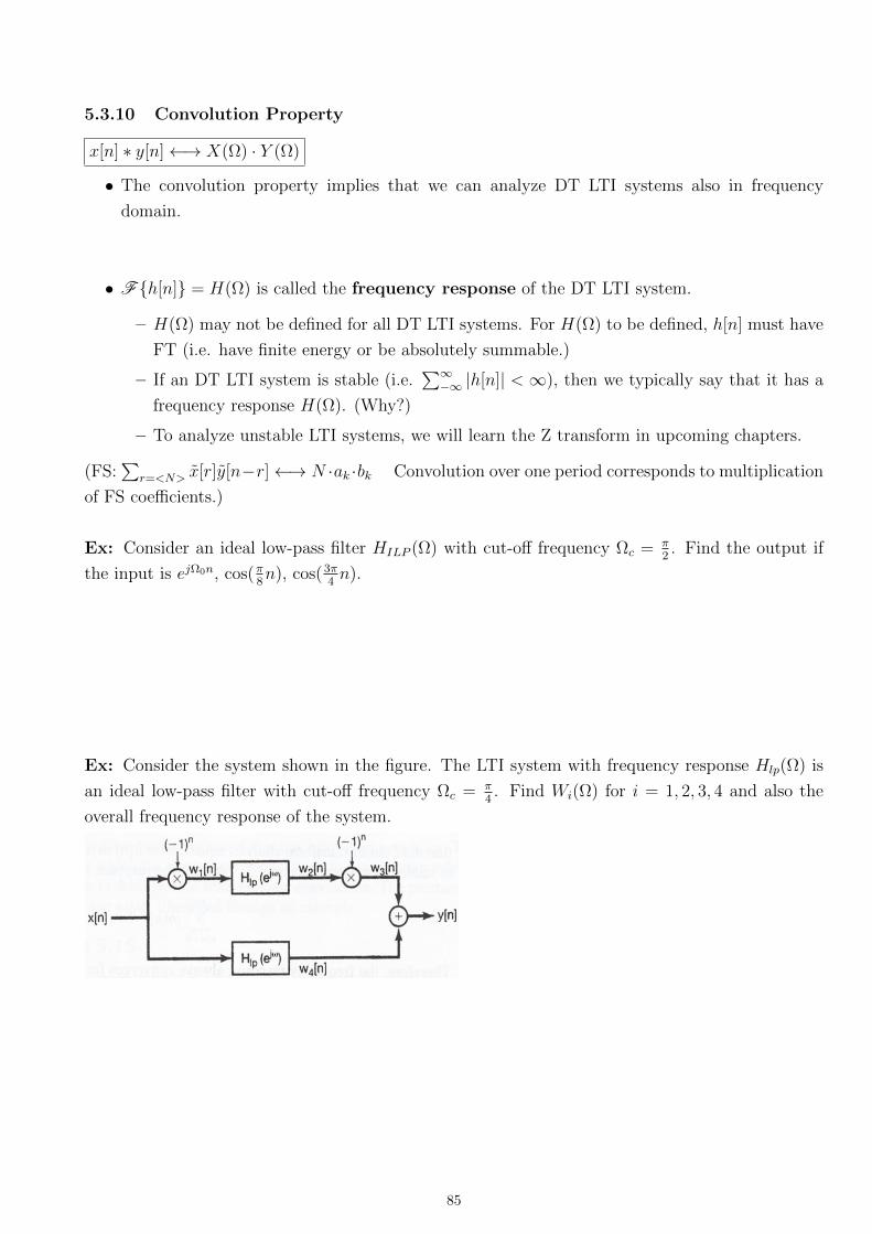
5.3.10 Convolution Property

x[n] ∗ y[n]←→ X(Ω) · Y (Ω)

• The convolution property implies that we can analyze DT LTI systems also in frequency

domain.

• Fh[n] = H(Ω) is called the frequency response of the DT LTI system.

– H(Ω) may not be defined for all DT LTI systems. For H(Ω) to be defined, h[n] must have

FT (i.e. have finite energy or be absolutely summable.)

– If an DT LTI system is stable (i.e.∑∞−∞ |h[n]| < ∞), then we typically say that it has a

frequency response H(Ω). (Why?)

– To analyze unstable LTI systems, we will learn the Z transform in upcoming chapters.

(FS:∑

r=<N> x[r]y[n−r]←→ N ·ak ·bk Convolution over one period corresponds to multiplication

of FS coefficients.)

Ex: Consider an ideal low-pass filter HILP (Ω) with cut-off frequency Ωc = π2. Find the output if

the input is ejΩ0n, cos(π8n), cos(3π

4n).

Ex: Consider the system shown in the figure. The LTI system with frequency response Hlp(Ω) is

an ideal low-pass filter with cut-off frequency Ωc = π4. Find Wi(Ω) for i = 1, 2, 3, 4 and also the

overall frequency response of the system.

85

5.3.11 Multiplication property

x[n] · y[n]←→ 1

2π

∫<2π>

X(θ)Y (Ω− θ)dθ (convolution over one period, i.e. 2π)

(FS: x[n] · y[n]←→∑

l=<N> albk−l convolution over one period )

Ex: Consider x1[n] =sin(3πn/4)

πn, x2[n] =

sin(πn/2)

πnand x[n] = x1[n] · x2[n]. Find X(Ω).

86

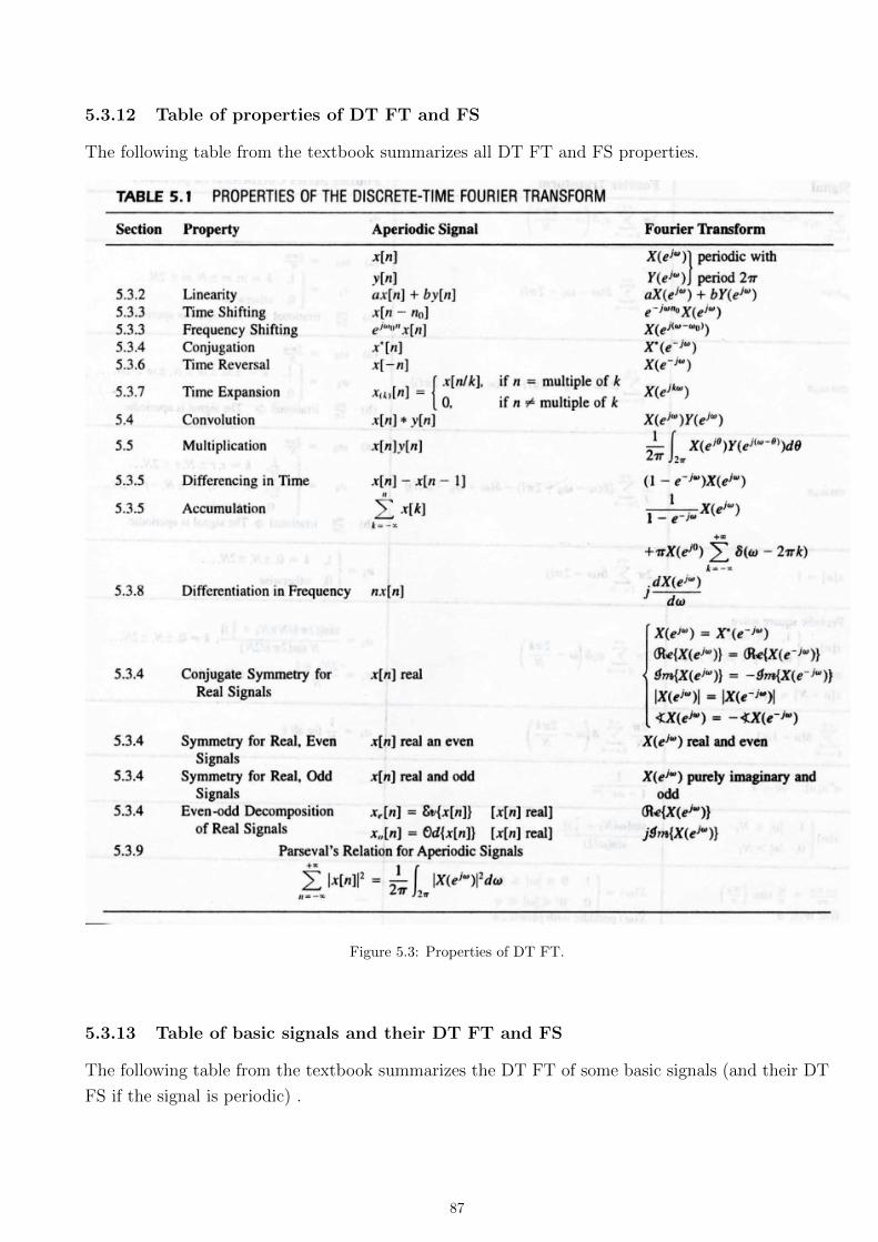
5.3.12 Table of properties of DT FT and FS

The following table from the textbook summarizes all DT FT and FS properties.

Figure 5.3: Properties of DT FT.

5.3.13 Table of basic signals and their DT FT and FS

The following table from the textbook summarizes the DT FT of some basic signals (and their DT

FS if the signal is periodic) .

87

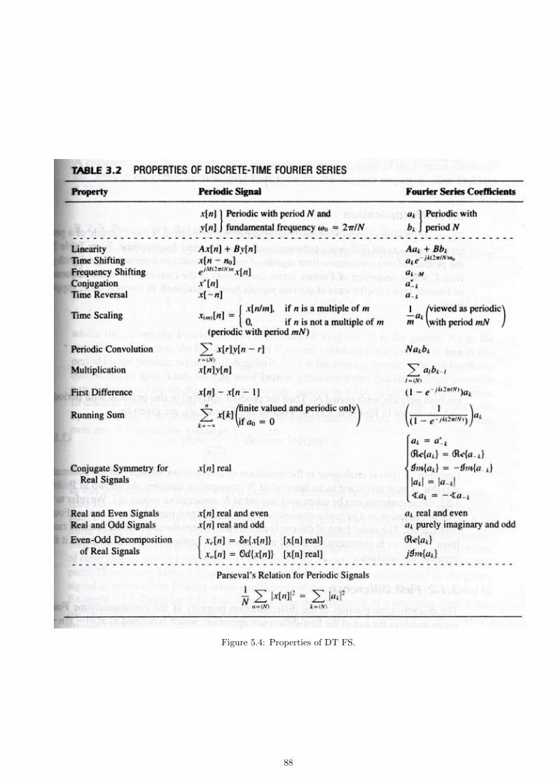
Figure 5.4: Properties of DT FS.

88

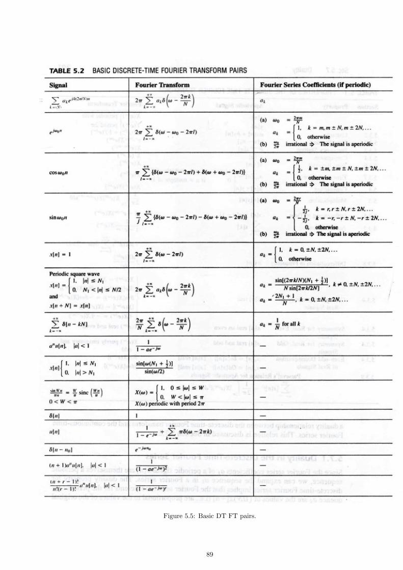
Figure 5.5: Basic DT FT pairs.

89

Chapter 6

Sampling

Contents

6.1 Representation of CT signals by its samples : the sampling theorem . . . . . . . . . . 91

6.1.1 Impulse-train sampling . . . . . . . . . . . . . . . . . . . . . . . . . . . . . . . . . . . . . . . 91

6.1.2 Sampling with a zero-order hold . . . . . . . . . . . . . . . . . . . . . . . . . . . . . . . . . 94

6.2 Effect of undersampling . . . . . . . . . . . . . . . . . . . . . . . . . . . . . . . . . . . . . . 95

6.3 DT processing of CT signals . . . . . . . . . . . . . . . . . . . . . . . . . . . . . . . . . . . 95

6.3.1 C/D conversion . . . . . . . . . . . . . . . . . . . . . . . . . . . . . . . . . . . . . . . . . . . 96

6.3.2 D/C conversion . . . . . . . . . . . . . . . . . . . . . . . . . . . . . . . . . . . . . . . . . . . 96

This chapter discusses sampling, the process in which samples from a CT signal xc(t) are taken to

generate a sequences of numbers ...,xc(0), xc(T ), xc(2T ), ..., called samples of the signal.

The samples can be seen as a DT signal (xd[n] = xc(nT )) and thus sampling can be seen as

converting a CT signal to a DT signal. Much of the importance of sampling comes from this role

as a bridge between CT and DT signals. In particular,

• nowadays, digital systems are preferred in many signal processing applications since they are

more flexible, cheaper and easily re-programmable, and

• signal processing of CT signals is done with digital systems by first sampling the CT signal,

then processing these samples as a DT signal, and then converting the processed DT signal

back to a CT signal.

90

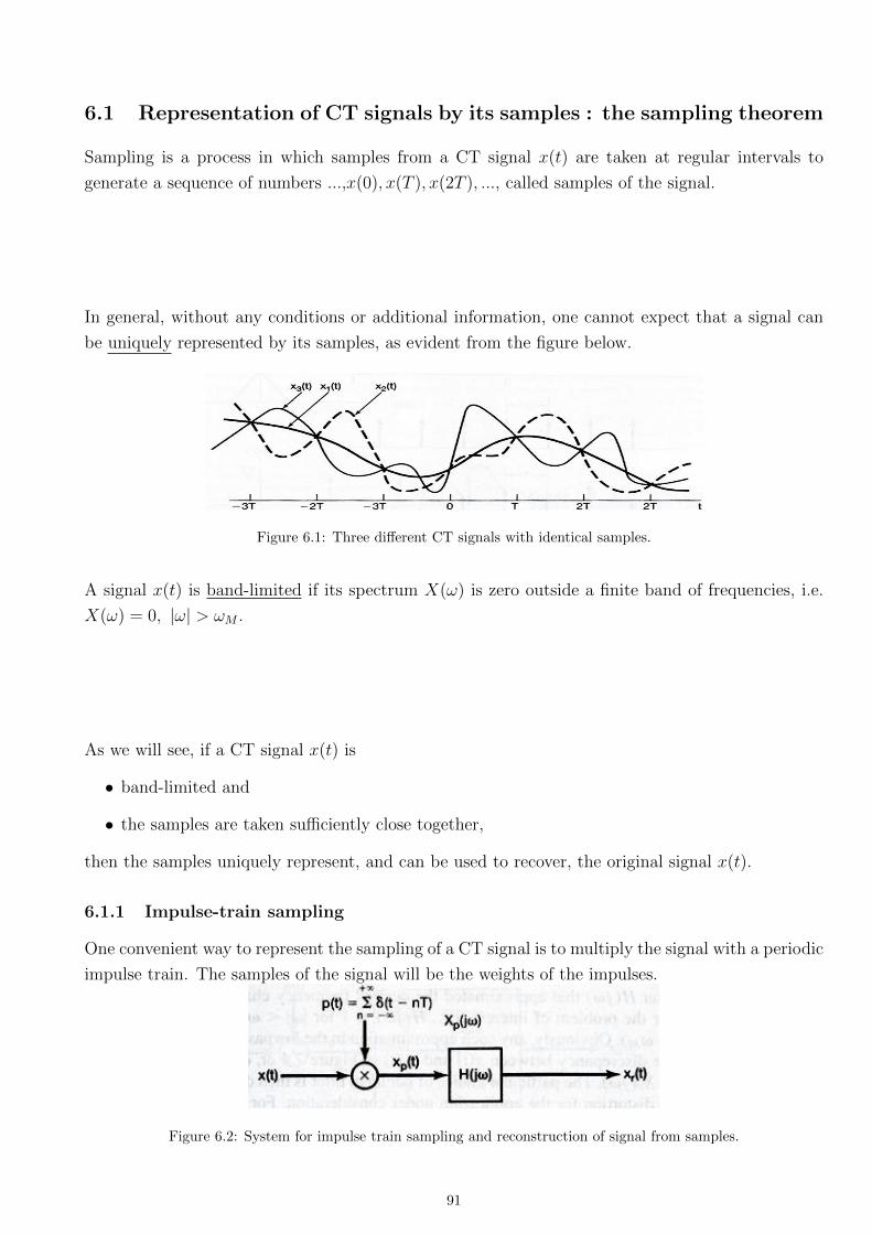
6.1 Representation of CT signals by its samples : the sampling theorem

Sampling is a process in which samples from a CT signal x(t) are taken at regular intervals to

generate a sequence of numbers ...,x(0), x(T ), x(2T ), ..., called samples of the signal.

In general, without any conditions or additional information, one cannot expect that a signal can

be uniquely represented by its samples, as evident from the figure below.

Figure 6.1: Three different CT signals with identical samples.

A signal x(t) is band-limited if its spectrum X(ω) is zero outside a finite band of frequencies, i.e.

X(ω) = 0, |ω| > ωM .

As we will see, if a CT signal x(t) is

• band-limited and

• the samples are taken sufficiently close together,

then the samples uniquely represent, and can be used to recover, the original signal x(t).

6.1.1 Impulse-train sampling

One convenient way to represent the sampling of a CT signal is to multiply the signal with a periodic

impulse train. The samples of the signal will be the weights of the impulses.

Figure 6.2: System for impulse train sampling and reconstruction of signal from samples.

91

Sampling in time domain :

Sampling in frequency domain :

Hence, when sampling frequency is sufficiently high, i.e. ωs > 2ωM , the original signal x(t) can

be perfectly recovered from xp(t) by an ideal low-pass filter with gain T and cut-off frequency ωc

chosen from the range ωM < ωc < ωs − ωM .

92

Sampling theorem :

Let x(t) be a band-limited signal with spectrum X(ω) = 0 for |ω| > ωM . Then x(t) is uniquely

determined by its samples x(nT ), n = 0,±1,±2, ... if

ωs > 2ωM

where ωs =2π

T. (The frequency 2ωM , which the sampling frequency ωs must exceed, is called

Nyquist sampling frequency.)

Given these samples, x(t) can be recovered by

• generating a periodic impulse train in which successive impulses have amplitudes that are

successive sample values,

• and processing this impulse train with an idea low-pass filter with gain T and cut-off frequency

ωc chosen from the range ωM < ωc < ωs − ωM .

Note that reconstructing the original CT signal x(t) from its samples requires an ideal low-pass

filter, which corresponds in time domain to convolving with a sinc() :

(Watch the demo on reconstruction by A.V. Oppenheim : https://youtu.be/_WV4JlBOQro?t=569)

In practical applications, since the sinc() signal is difficult to implement, a simpler low-pass filter

may be used, which can give a reconstructed signal xr(t) not exactly equal to original x(t) but the

error may be tolerated in some applications.

(Demo on linear reconstruction by A.V. Oppenheim : https://youtu.be/_WV4JlBOQro?t=1301)

93

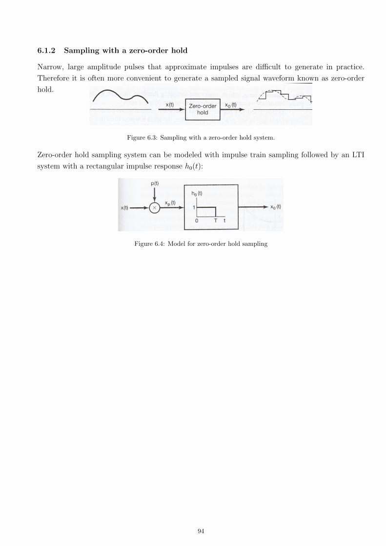
6.1.2 Sampling with a zero-order hold

Narrow, large amplitude pulses that approximate impulses are difficult to generate in practice.

Therefore it is often more convenient to generate a sampled signal waveform known as zero-order

hold.

Figure 6.3: Sampling with a zero-order hold system.

Zero-order hold sampling system can be modeled with impulse train sampling followed by an LTI

system with a rectangular impulse response h0(t):

Figure 6.4: Model for zero-order hold sampling

94

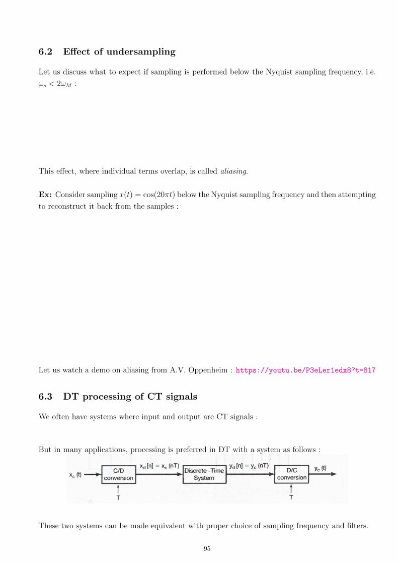
6.2 Effect of undersampling

Let us discuss what to expect if sampling is performed below the Nyquist sampling frequency, i.e.

ωs < 2ωM :

This effect, where individual terms overlap, is called aliasing.

Ex: Consider sampling x(t) = cos(20πt) below the Nyquist sampling frequency and then attempting

to reconstruct it back from the samples :

Let us watch a demo on aliasing from A.V. Oppenheim : https://youtu.be/P3eLer1edx8?t=817

6.3 DT processing of CT signals

We often have systems where input and output are CT signals :

But in many applications, processing is preferred in DT with a system as follows :

These two systems can be made equivalent with proper choice of sampling frequency and filters.

95

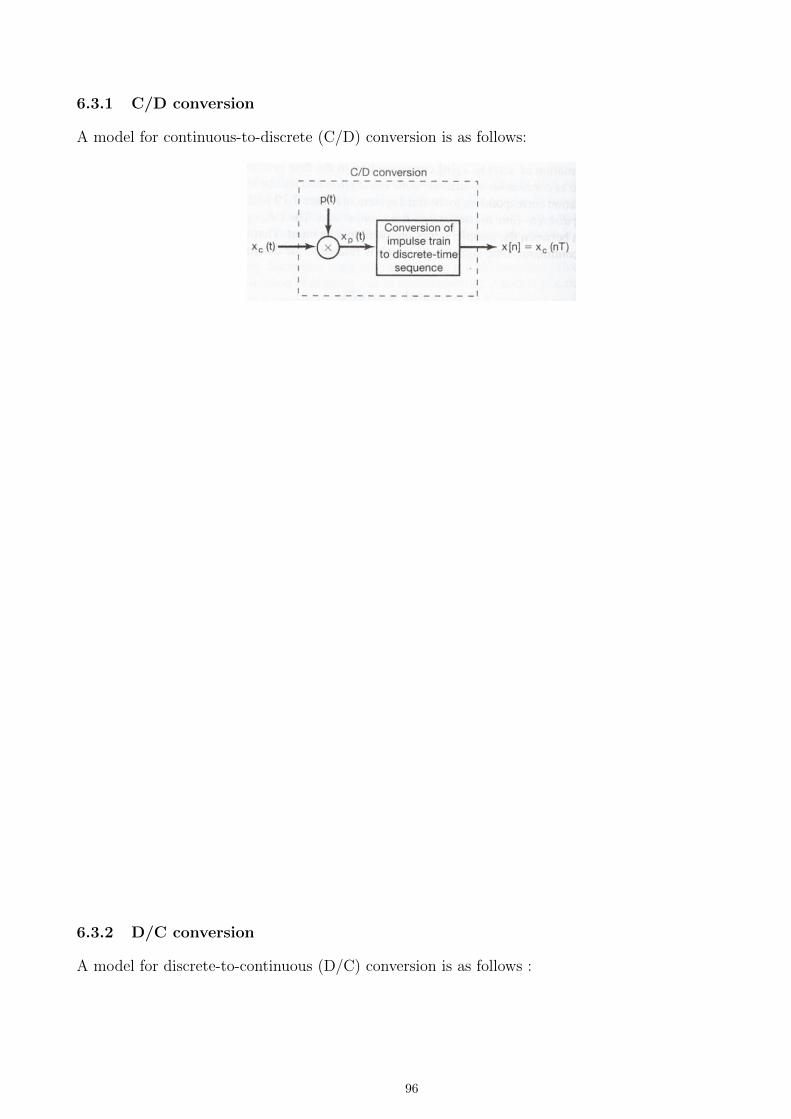
6.3.1 C/D conversion

A model for continuous-to-discrete (C/D) conversion is as follows:

6.3.2 D/C conversion

A model for discrete-to-continuous (D/C) conversion is as follows :

96

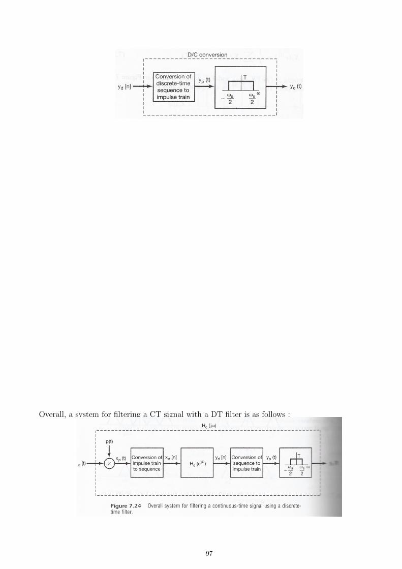
Overall, a system for filtering a CT signal with a DT filter is as follows :

97

Chapter 7

The Z-transform

Contents

7.1 The Z transform and its region of convergence (ROC) . . . . . . . . . . . . . . . . . . . 99

7.2 Properties of ROC . . . . . . . . . . . . . . . . . . . . . . . . . . . . . . . . . . . . . . . . . 102

7.3 Inversion of Z transforms . . . . . . . . . . . . . . . . . . . . . . . . . . . . . . . . . . . . . 105

7.4 Properties of Z transform . . . . . . . . . . . . . . . . . . . . . . . . . . . . . . . . . . . . 106

7.4.1 Linearity . . . . . . . . . . . . . . . . . . . . . . . . . . . . . . . . . . . . . . . . . . . . . . 106

7.4.2 Time Shift . . . . . . . . . . . . . . . . . . . . . . . . . . . . . . . . . . . . . . . . . . . . . 107

7.4.3 Scaling in z domain (Frequency shifting) . . . . . . . . . . . . . . . . . . . . . . . . . . . . . 107

7.4.4 Time Reversal . . . . . . . . . . . . . . . . . . . . . . . . . . . . . . . . . . . . . . . . . . . 107

7.4.5 Conjugation . . . . . . . . . . . . . . . . . . . . . . . . . . . . . . . . . . . . . . . . . . . . . 107

7.4.6 Convolution . . . . . . . . . . . . . . . . . . . . . . . . . . . . . . . . . . . . . . . . . . . . . 108

7.4.7 Differentiation . . . . . . . . . . . . . . . . . . . . . . . . . . . . . . . . . . . . . . . . . . . 108

7.4.8 The initial value theorem . . . . . . . . . . . . . . . . . . . . . . . . . . . . . . . . . . . . . 108

7.4.9 Table of Z transform properties and some common z transform pairs . . . . . . . . . . . . . 109

7.5 LTI Systems and the Z transform . . . . . . . . . . . . . . . . . . . . . . . . . . . . . . . . 110

7.5.1 Causality . . . . . . . . . . . . . . . . . . . . . . . . . . . . . . . . . . . . . . . . . . . . . . 110

7.5.2 Stability . . . . . . . . . . . . . . . . . . . . . . . . . . . . . . . . . . . . . . . . . . . . . . . 111

In the preceding chapters, we have seen that Fourier series and transform representations are very

useful in the study of many problems involving signals and LTI systems. This is mainly due to the

facts that Fourier tools represent signals as a linear combination of complex exponentials of the

form ejωt in CT and ejΩn in DT, which are eigenfunctions of LTI systems.

However, the eigenfunction property also applies to more general complex exponentials of the form

est with s = α + jω in CT and zn with z = rejΩ in DT. This observation leads to generalization

of the CT and DT Fourier transforms known as the Laplace transform in CT and z transform in DT.

As we will see, the Laplace and z transform have many of the beautiful properties of the Fourier

transform but also provide additional tools and insights. In particular, for signals for which the

98

Fourier transforms do not exist, the Laplace or z transform may converge/exist, and thus they can

be very useful in the stability analysis of systems.

This chapter discusses the z transform and the next chapter will discuss the Laplace transform.

7.1 The Z transform and its region of convergence (ROC)

Remember that DT complex exponentials of the general form zn = (rejΩ)n are eigenfunctions of DT

LTI systems with eigenvalues given by H(z) =∑∞

k=−∞ h[k]z−k where h[n] is the impulse response

of the system:

The eigenvalue expression provides the definition of the z transform of a signal x[n] where z is a

complex number :

X(z) =∞∑

n=−∞

x[n]z−n

We again will use shorthand notations for the z transform of a signal x[n]:

• Z x[n]

• x[n]←→ X(z)

The z transform is a generalization of the Fourier transform and they are related as follows :

• X(z)|z=rejΩ = Fx[n]r−n

• X(z)|z=ejΩ = Fx[n] (i.e. z transform reduces to FT for values of z on the unit circle of the

z-plane)

The above relation indicates that the convergence/existence of z transform, requires the conver-

gence/existence Fx[n]r−n,

99

• which happens when x[n]r−n is absolutely summable, i.e.∑∞−∞ |x[n]r−n| <∞

• and thus z transform X(z) converges/exists for some values of r and does not for others.

Region of Convergence (ROC) : A range of r (note that |z| = r) values for which z transform X(z)

converges.

Ex: x[n] = αnu[n]. Find X(z) and its ROC.

Note that the above relation between z transform and Fourier transform are valid if |z| = r is

contained in the ROC of X(z) :

In particular, if the ROC of X(z) contains the unit circle |z| = r = 1, then the DT FT X(Ω) exists

and is given by X(z)|z=ejΩ :

Ex: Previous example with α = 12

and α = 32.

100

Ex: x[n] = −αnu[−n− 1]. Find X(z) and its ROC.

Notes :

• It is helpful to remember the following frequently used signal and z transform pairs :

αnu[n] ←→ z

z − α, ROC : |z| > |α|

−αnu[−n− 1] ←→ z

z − α, ROC : |z| < |α|

• The specification of the z transform requires both

– the algebraic expression for X(z)

– and the associated ROC.

(Without the ROC, X(z) by itself does not uniquely specify a signal x[n].)

Ex: x[n] = (12)nu[n] + (1

3)nu[n]. Find X(z) and its ROC.

101

Ex: x[n] = −(12)nu[−n− 1] + (1

3)nu[n]. Find X(z) and its ROC.

7.2 Properties of ROC

Property 1 : The ROC of X(z) depends only on |z| = r and therefore consists of a ring in the

z-plane centered at the origin.

Reason :

• The relation X(z)|z=rejΩ = Fx[n]r−n indicates that the convergence/existence of z trans-

form X(z), requires the convergence/existence Fx[n]r−n, which happens when x[n]r−n is

absolutely summable, i.e.∑∞−∞ |x[n]r−n| =

∑∞−∞ |x[n]|r−n <∞.

• Thus, ROC of X(z) depends only on r = |z| and is independent of Ω.

Property 2 : For rational X(z), the ROC does not contain any poles.

Reason :

• Rational X(z) means X(z) is a ratio of polynomials of z.

• A pole of X(z) is a root of the denominator and a zero of X(z) is a root of the numerator.

• X(z) is infinite at a pole and hence does not converge at a pole.

Property 3 : If x[n] is of finite duration, then the ROC is the entire z-plane except possibly z = 0

and/or z =∞.

102

Reason :

• A finite duration sequence has only a finite number of nonzero samples, e.g.

• For finite z, X(z) is a finite sum of ...

• If N1 < 0 and N2 > 0, then ...

• If 0 < N1 < N2, then ...

• If N1 < N2 < 0, then ...

Property 4 : If x[n] is a right-sided sequence, then the ROC is the outside of a circle centered at

the origin (excluding possibly z =∞).

Reason :

• A sight-sided sequence is of the form ...

• Some r is in ROC of X(z) if X(z) = Fx[n]r−n converges which happens if∑∞−∞ |x[n]|r−n <

∞.

• If some r0 is in the ROC of X(z), i.e.∑∞

N1|x[n]r−n0 | <∞, then for N1 > 0 and some r1 > r0,

we have∑∞

N1|x[n]r−n1 | <∞ since ...

– Hence, Fx[n]r−n1 converges and thus |z| = r1 is also in the ...

– Thus the ROC must be the outside of a circle.

– Note that ifN1 < 0, there is a finite sum of terms coming from negative n (i.e.∑0

N1|x[n]r−n1 |),

which will not cause a problem for convergence except possibly at for z =∞.

Property 5 : If x[n] is a left-sided sequence, then the ROC is the inside of a circle centered at the

origin (excluding possibly z = 0).

Reason is similar to the previous property’s.

Property 6 : If x[n] is a two-sided sequence, then the ROC consists of a ring or is empty.

Reason :

• A two-sided sequence can be considered as the sum of ...

• The ROC of X(z) of the sum of sequences is the intersection of the ROCs of the z transforms

of each sequence.

103

Ex: x[n] =

2n, n < 0

(13)n, n = 0, 2, 4, ..

0, n = 1, 3, 5, ...

. Find X(z) and its ROC.

Property 7 : If X(z) is rational, then its ROC is bounded by the poles or extends to infinity.

Reason :

• A signal x[n] with rational X(z) consist of a linear combination of exponentials αnu[n] or

−αnu[−n− 1] which have ROCs bounded by their poles.

• The ROC of X(z) of the linear combination of exponentials thus is the intersection of ROCs

bounded by poles.

Property 8 : If X(z) is rational and x[n] is right-sided, then its ROC is the outside of the outer-

most pole. (Furthermore, if x[n] is also causal, then the ROC also includes z =∞.)

Reason : ...

Property 9 : If X(z) is rational and x[n] is left-sided, then its ROC is the inside of the innermost

pole. (Furthermore, if x[n] is also anti-causal (i.e. x[n] = 0 for n > 0), then the ROC also includes

z = 0.)

Reason : ...

104

7.3 Inversion of Z transforms

The inverse z transform expression contains integration around a circular contour on the z-plane

and is typically difficult to compute and will not be applied in this course. However, there are a

number of alternative procedures for obtaining a sequence from its z transform and associated ROC.

One useful procedure for rational X(z) is to expand X(z) into a partial-fraction expansion, and

then to recognize the sequence associated with each term in the expansion.

Ex: X(z) =3z

(2− z)(2z − 1), ROC:1

2< |z| < 2. Find x[n].

Another procedure is to use the power series expansion of z transform and determine x[n] by

inspection.

Ex: X(z) = 4z2 + 2 + 3z−1, ROC:0 < |z| <∞. Find x[n].

105

Power series expansion can be very useful for some non-rational X(z).

Ex: X(z) = log(1 + z−1), ROC:|z| > 1. Find x[n].

7.4 Properties of Z transform

To discuss the z transform properties, we use the same convenient shorthand notation we used for

Fourier transform properties. In other words, to indicate the pairing of a signal and its z transform,

we use :

• signal ←→ z transform ( e.g. x[n]←→ X(z) )

We sometimes also refer to a z transform with the following notation :

• Z signal ( e.g. X(z) = Z x[n], ROC : |z| > a)

For the following properties, let us assume that we have two signals x[n] and y[n] with corresponding

z transforms X(z) and Y (z), and ROCs Rx and Ry, respectively, i.e.

x[n]←→ X(z), ROC : Rx and y[n]←→ Y (z), ROC : Ry.

7.4.1 Linearity

ax[n] + by[n]←→ aX(z) + bY (z), ROC : Rx ∩Ry

106

7.4.2 Time Shift

x[n− n0]←→ z−n0X(z), ROC : Rx except for possible inclusion or deletion of origin or infinity.

Ex: x1[n] = −δ[n+ 1] + δ[n] and x2[n] = x1[n− 1]. Find the z transforms and associated ROCs.

7.4.3 Scaling in z domain (Frequency shifting)

zn0x[n]←→ X( zz0

), ROC : |z0|Rx = z : zz0∈ Rx

Important special case for z0 = 1 · ejω0n:

ejω0nx[n]←→

Ex: Rx : 12< |z| < 5 and |z0| = 3. Find |z0|Rx.

7.4.4 Time Reversal

x[−n]←→ X(1z), ROC : 1

Rx= z : 1

z∈ Rx

Ex: Rx : 12< |z| < 5. Find 1

Rx.

7.4.5 Conjugation

x∗[n]←→ X∗(z∗), ROC : Rx

If x[n] is real, (i.e. x[n] = x∗[n])

• X(z) = X∗(z∗)

• thus, if X(z) has a pole (zero) at z = z0, then it must also have a pole (zero) at the complex

conjugate point z = z∗0 .

107

Ex: Consider X(z) = A(z)z − bz − a

. Find X∗(z∗) and its poles. Show that if X(z) = X∗(z∗), then

the poles and zeros must appear in complex conjugate pairs.

7.4.6 Convolution

x[n] ∗ y[n]←→ X(z) · Y (z), ROC : at least Rx ∩Ry (pole zero cancellations may occur)

Ex: Consider x1[n] and x2[n] plotted below and find z transform of x1[n] ∗ x2[n].

7.4.7 Differentiation

nx[n]←→ −z ddzX(z), ROC : Rxwith possible inclusion ofz = 0.

Ex: X(z) =az−1

(1− az−1)2, |z| > a. Determine x[n].

7.4.8 The initial value theorem

x[0] = limz→∞X(z) if x[n] is causal, i.e. x[n] = 0 for n < 0.

108

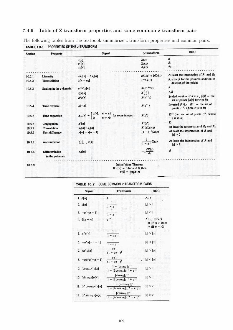
7.4.9 Table of Z transform properties and some common z transform pairs

The following tables from the textbook summarize z transform properties and common pairs.

109

7.5 LTI Systems and the Z transform

The z transform plays an important role in the analysis and representation of DT LTI systems :

• From the convolution property, we have : Y (z) = H(z) ·X(z)

• Z h[n] = H(z) is called the system function or transfer function of the LTI system.

• If ROC of H(z) includes the unit circle, then for z on the unit circle (i.e. |z| = r = 1), H(z)

reduces to frequency response H(Ω) = Fh[n] of the system,

– i.e. |z| = 1 ∈ ROC −→ H(z)|z=1·ejΩ = H(Ω)

• DT complex exponentials zn are eigenfunctions of DT LTI systems and the eigenvalues are

given by the system function H(z).

Many properties of and LTI system can be tied directly to characteristics of the poles, zeros and

ROC of H(z), as we discus below.

7.5.1 Causality

Property 1 : A DT LTI system is causal if and only if the ROC of H(z) is the outside of a circle,

including infinity.

Reason :

• Impulse response h[n] of a causal system is right-sided, which implies that ROC of H(z) must

be ...

• H(z) =∑∞

n=0 h[n]z−n = h[0] + h[1]z−1 + h[2]z−2 + ... implies that ROC includes ...

Property 2 : A DT LTI system with rational H(z) is causal if and only if

• the ROC of H(z) is the outside of the outermost pole

• order(a(z))≤ order(b(z)) where H(z) =a(z)

b(z).

Reason :

• Property 8 of ROC properties

• If order(a(z))> order(b(z)), consider for example H(z) =2z2 + 1

z − 1=...

110

7.5.2 Stability

Property 1 : A DT LTI system is stable if and only if the ROC of H(z) includes the unit circle,

|z| = 1.

Reason :

• A DT LTI system is stable ⇐⇒

•∑∞

n=−∞ |h[n]| <∞ ⇐⇒ Fh[n] = H(Ω) converges (1st Dirichlet condition)

• H(Ω) = H(z)|z=1·ejΩ

Property 2 : A causal DT LTI system with rational H(z) is stable if and only if all poles of

H(z) lie inside the unit circle (i.e. all poles have magnitudes smaller than 1.)

Reason :

• For a causal system with rational H(z), ROC is ...

• For this ROC to include unit circle, ...

Ex: An LTI system satisfies the following difference equation :

y[n]− 1

2y[n− 1] = x[n] +

1

3x[n− 1].

Find the system function H(z). Find all possible ROCs for this H(z). For each possible ROC, find

the corresponding h[n].

111

Ex: Consider a stable and causal system with impulse response h[n] and rational system function

H(z). It is known that H(z) contains a pole at z = 12

and a zero somewhere on the unit circle. The

precise number and locations of other poles and zeros are unknown. Find if each of the following is

True, False or cannot be surely determined.

• F(12)nh[n] converges

• H(Ω) = 0 for some Ω

• h[n] has finite duration

• h[n] is real

• g[n] = n(h[n] ∗ h[n]) is the impulse response of a stable system.

112

Chapter 8

The Laplace transform

Contents

8.1 The Laplace transform and its region of convergence (ROC) . . . . . . . . . . . . . . . 113

8.2 Properties of ROC . . . . . . . . . . . . . . . . . . . . . . . . . . . . . . . . . . . . . . . . . 117

8.3 Inversion of Laplace transforms . . . . . . . . . . . . . . . . . . . . . . . . . . . . . . . . . 119

8.4 Properties of Laplace transform . . . . . . . . . . . . . . . . . . . . . . . . . . . . . . . . . 120

8.4.1 Linearity . . . . . . . . . . . . . . . . . . . . . . . . . . . . . . . . . . . . . . . . . . . . . . 120

8.4.2 Time Shift . . . . . . . . . . . . . . . . . . . . . . . . . . . . . . . . . . . . . . . . . . . . . 120

8.4.3 Frequency Shift . . . . . . . . . . . . . . . . . . . . . . . . . . . . . . . . . . . . . . . . . . . 121

8.4.4 Time Scaling . . . . . . . . . . . . . . . . . . . . . . . . . . . . . . . . . . . . . . . . . . . . 121

8.4.5 Conjugation . . . . . . . . . . . . . . . . . . . . . . . . . . . . . . . . . . . . . . . . . . . . . 121

8.4.6 Convolution . . . . . . . . . . . . . . . . . . . . . . . . . . . . . . . . . . . . . . . . . . . . . 121

8.4.7 Differentiation in s domain . . . . . . . . . . . . . . . . . . . . . . . . . . . . . . . . . . . . 121

8.4.8 Differentiation in time domain . . . . . . . . . . . . . . . . . . . . . . . . . . . . . . . . . . 122

8.4.9 Integration in time domain . . . . . . . . . . . . . . . . . . . . . . . . . . . . . . . . . . . . 122

8.4.10 Initial and Final Value Theorem . . . . . . . . . . . . . . . . . . . . . . . . . . . . . . . . . 122

8.4.11 Table of Laplace transform properties and common Laplace transform pairs . . . . . . . . . 123

8.5 LTI Systems and the Laplace transform . . . . . . . . . . . . . . . . . . . . . . . . . . . . 124

8.5.1 Causality . . . . . . . . . . . . . . . . . . . . . . . . . . . . . . . . . . . . . . . . . . . . . . 124

8.5.2 Stability . . . . . . . . . . . . . . . . . . . . . . . . . . . . . . . . . . . . . . . . . . . . . . . 125

This chapter discusses the Laplace transform, which plays a role for CT signals that is similar to

the role of z transform for DT signals.

8.1 The Laplace transform and its region of convergence (ROC)

Remember that CT complex exponentials of the general form est = e(σ+jω)t are eigenfunctions of CT

LTI systems with eigenvalues given by H(s) =∫∞t=−∞ h(t)e−stdt where h(t) is the impulse response

of the system:

113

The eigenvalue expression provides the definition of the Laplace transform of a signal x(t) where s

is a complex number :

X(s) =

∫ ∞t=−∞

x(t)e−stdt

We again will use shorthand notations for the Laplace transform of a signal x(t):

• L x(t)

• x(t)←→ X(s)

The Laplace transform is a generalization of the Fourier transform and they are related as follows :

• X(s)|s=σ+jω = Fx(t)e−σt

• X(s)|s=jω = Fx(t) (i.e. Laplace transform reduces to FT for values of s on the imaginary

axis of the s-plane)

The above relation indicates that the convergence/existence of Laplace transform, requires the

convergence/existence Fx(t)e−σt,

• which happens when x(t)e−σt is absolutely integrable, i.e.∫∞−∞ |x(t)e−σt| <∞

• and thus Laplace transform X(s) converges/exists for some values of σ and does not for others.

Region of Convergence (ROC) : A range of σ (note that σ = Res) values for which Laplace

transform X(s) converges.

Ex: x(t) = e−αtu(t). Find X(s) and its ROC.

114

Note that the above relation between Laplace transform and Fourier transform are valid ifRes = σ

is contained in the ROC of X(s) :

In particular, if the ROC of X(s) contains the jω-axis (Res = 0), then the CT FT X(ω) exists

and is given by X(s)|s=jω :

Ex: Previous example with α = 2 and α = −2.

Ex: x(t) = −e−αtu(−t). Find X(s) and its ROC.

115

Notes :

• It is helpful to remember the following frequently used signal and Laplace transform pairs :

e−αtu(t) ←→ 1

s+ α, ROC : Res > α

−e−αtu(−t) ←→ 1

s+ α, ROC : Res < α

• The specification of the Laplace transform requires both

– the algebraic expression for X(s)

– and the associated ROC.

(Without the ROC, X(s) by itself does not uniquely specify a signal x(t).)

Ex: x(t) = 3e−2tu(t)− 2e−tu(t). Find X(s) and its ROC.

Ex: x(t) = e−2tu(t) + e−t cos(3t)u(t). Find X(s) and its ROC.

116

8.2 Properties of ROC

Property 1 : The ROC of X(s) depends only on Res and therefore consists of strips parallel

to the jω-axis in the s-plane.

Reason :

• The relation X(s)|s=σ+jω = Fx(t)e−σt indicates that the convergence/existence of Laplace

transformX(s), requires the convergence/existence Fx(t)e−σt, which happens when x(t)e−σt

is absolutely integrable, i.e.∫∞−∞ |x(t)e−σt|dt =

∫∞−∞ |x(t)|e−σtdt <∞.

• Thus, ROC of X(s) depends only on σ = Res and is independent of ω.

Property 2 : For rational X(s), the ROC does not contain any poles.

Reason :

• Rational X(s) means X(s) is a ratio of polynomials of s.

• A pole of X(s) is a root of the denominator and a zero of X(s) is a root of the numerator.

• X(s) is infinite at a pole and hence does not converge at a pole.

Property 3 : If x(t) is of finite duration, then the ROC is either empty or the entire s-plane.

Reason :

• A finite duration signal x(t) is nonzero only a finite interval, e.g.

• Let us assume that X(s) converges for one σ0 = Res, then ...

• Then the ROC must also include any arbitrary vertical line at any σ1, since

–∫ T2

T1|x(t)|e−σ1tdt = ...

– and therefore ...

Property 4 : If x(t) is a right-sided sequence, then the ROC is either empty or to the right of a

vertical line.

Reason :

• A right-sided signal is such that x(t) = 0, t < T1 e.g.

117

• Let us assume that X(s) converges for one σ0 = Res, then ...

• Then the ROC must also include the vertical line at any σ1 > σ0, since

–∫∞T1|x(t)|e−σ1tdt = ...

– and therefore ...

Property 5 : If x(t) is a left-sided sequence, then the ROC is either empty or to the left of a

vertical line.

Reason is similar to the previous property’s.

Property 6 : If x(t) is a two-sided signal, then the ROC is either empty or consists of a strip

bounded from right and left.

Reason :

• A two-sided signal can be considered as the sum of ...

• The ROC of X(s) of the sum of sequences is the intersection of the ROCs of the Laplace

transforms of each sequence.

Ex: x(t) = e−bt. Find X(s) and the ROC if b > 0 and b < 0.

Property 7 : If X(s) is rational, then its ROC is bounded by the poles or extends to infinity.

Reason :

118

• A signal x(t) with rational X(s) consist of a linear combination of exponentials e−αtu(t) or

−e−αtu(−t) which have ROCs bounded by their poles.

• The ROC of X(s) of the linear combination of exponentials thus is the intersection of ROCs

bounded by poles.

Property 8 : If X(s) is rational and x(t) is right-sided, then its ROC is the right side of the right-

most pole. If X(s) is rational and x(t) is left-sided, then its ROC is the left side of the left-most pole.

Reason : ...

8.3 Inversion of Laplace transforms

The inverse Laplace transform expression contains integration around a contour on the s-plane and

is typically difficult to compute and will not be applied in this course.

However, one useful alternative procedure for obtaining a signal from its Laplace transform and

associated ROC is to expand X(s) into a partial-fraction expansion, and then to recognize the

signal associated with each term in the expansion.

Ex: X(s) =2

s2 − 4, ROC:Res > 2. Find x(t).

Ex: X(s) =1

(s+ 1)(s+ 2). Find all possible ROCs for this X(s). For each possible ROC, find the

corresponding x(t).

119

8.4 Properties of Laplace transform

To discuss the Laplace transform properties, we use the same convenient shorthand notation we

used for Fourier transform properties. In other words, to indicate the pairing of a signal and its

Laplace transform, we use :

• signal ←→ Laplace transform ( e.g. x(t)←→ X(s) )

We sometimes also refer to a Laplace transform with the following notation :

• L signal ( e.g. X(s) = L x(t), ROC : Res > a)

For the following properties, let us assume that we have two signals x(t) and y(t) with corresponding

Laplace transforms X(s) and Y (s), and ROCs Rx and Rx, respectively, i.e.

x(t)←→ X(s), ROC : Rx and y(t)←→ Y (s), ROC : Ry.

8.4.1 Linearity

ax(t) + by(t)←→ aX(s) + bY (s), ROC : Rx ∩Ry

8.4.2 Time Shift

x(t− t0)←→ e−st0X(s), ROC : Rx

120

8.4.3 Frequency Shift

es0tx(t)←→ X(s− s0), ROC : Res+Rx = s : s− s0 ∈ Rx

Ex: ROC of X(s) is Res > 2. Find L x(t− 1) and the associated ROC.

8.4.4 Time Scaling

x(at)←→ 1

|a|X( s

a), ROC :

Rx

a= s : s

a∈ Rx

Ex: ROC of X(s) is −3 < Res < 2. Find L x(2t) and the associated ROC.

8.4.5 Conjugation

x∗(t)←→ X∗(s∗), ROC : Rx

If x(t) is real, (i.e. x(t) = x∗(t))

• X(s) = X∗(s∗)

• thus, if X(s) has a pole (zero) at s = s0, then it must also have a pole (zero) at the complex

conjugate point s = s∗0.

8.4.6 Convolution

x(t) ∗ y(t)←→ X(s) · Y (s), ROC : at least Rx ∩Ry (pole zero cancellations may occur)

8.4.7 Differentiation in s domain

−tx(t)←→ d

dsX(s), ROC : Rx

121

Ex: x(t) = te−atu(t). Find X(s) and ROC.

8.4.8 Differentiation in time domain

d

dtx(t)←→ sX(s), ROC : Rxwith possible pole zero cancellation ats = 0.

8.4.9 Integration in time domain∫ t−∞ x(τ)dτ ←→ 1

sX(s), ROC : At leatst Rx ∩Res > 0.

8.4.10 Initial and Final Value Theorem

Under the conditions that x(t) = 0 for t < 0 and x(t) contains no impulses or higher order singu-

larities at the origin :

IVT : x(0+) = lims→∞ sX(s) FVT : limt→∞ x(t) = lims→0 sX(s)

IVT and FVT can be useful in checking correctness of Laplace transform calculations for a signal.

Ex: In a previous example we found that X(s) =2s2 + 5s+ 12

(s2 + 2s+ 10)(s+ 2)for x(t) = e−2tu(t) +

e−t cos(3t)u(t). We can check if the calculated X(s) is correct by IVT :

122

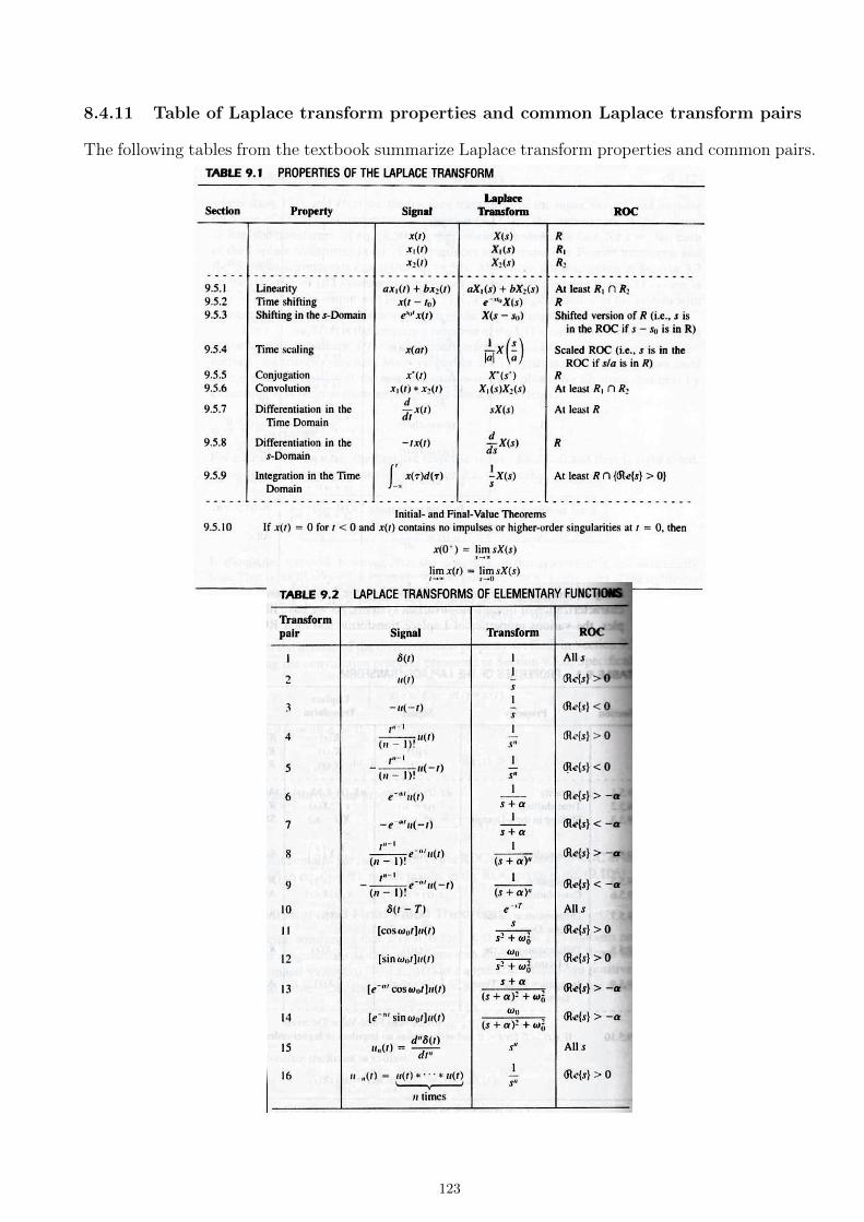
8.4.11 Table of Laplace transform properties and common Laplace transform pairs

The following tables from the textbook summarize Laplace transform properties and common pairs.

123

8.5 LTI Systems and the Laplace transform

The Laplace transform plays an important role in the analysis and representation of CT LTI systems:

• From the convolution property, we have : Y (s) = H(s) ·X(s)

• L h(t) = H(s) is called the system function or transfer function of the LTI system.

• If ROC of H(s) includes the jω-axis (i.e. Res = 0), H(s) reduces to frequency response

H(ω) = Fh(t) of the system,

– i.e. Res = 0 ∈ ROC −→ H(s)|s=0+jω = H(ω)

• CT complex exponentials est are eigenfunctions of CT LTI systems and the eigenvalues are

given by the system function H(s).

Many properties of and LTI system can be tied directly to characteristics of the poles, zeros and

ROC of H(s), as we discus below.

8.5.1 Causality

Property 1 : The ROC associated with H(s) of a causal CT LTI system is a right-half plane. (The

converse is not necessarily true!)

Reason :

• Impulse response h(t) of a causal system is right-sided, which implies that ROC of H(s) must

be ...

Ex: Consider causal LTI system with h(t) = e−tu(t). Find H(s) and the associated ROC.

Next, consider H(s) =es

s+ 1, with ROC:Res > −1. Find h(t).

Property 2 : A CT LTI system with rational H(s) is causal if and only if the ROC of H(s) is

the right side of the right most pole.

124

8.5.2 Stability

Property 1 : A CT LTI system is stable if and only if the ROC of H(s) includes the entire

jω-axis (i.e. Res = 0 line).

Reason :

• A CT LTI system is stable ⇐⇒

•∫∞t=−∞ |h(t)| <∞ ⇐⇒ Fh(t) = H(ω) converges (1st Dirichlet condition)

• H(ω) = H(s)|s=0+jω

Property 2 : A causal CT LTI system with rational H(s) is stable if and only if all poles of

H(s) lie on the left half of the s-plane (i.e. all poles have negative real parts Res < 0.)

Reason :

• For a causal system with rational H(s), ROC is ...

• For this ROC to include the jω-axis, ...

Ex: For LTI system with H(s) =s− 1

(s+ 1)(s− 2− j)(s− 2 + j), determine all possible ROCs. For

each possible ROC, discuss if the system causal and/or stable.

Ex: For an input x(t) = e3tu(t), the output of an LTI system is y(t) = [e−t − e−2t]u(t). Determine

system function H(s).

• Can you also find the ROC of H(s) and then h(t) ?

• Is the system causal and/or stable ?

125

• Find the differential equation that can represent this LTI system.

Ex: Consider a stable and causal system with impulse response h(t) and rational system function

H(s). It is known that H(s) contains a pole at s = −2 and does not have a zero at the origin. The

precise number and locations of other poles and zeros are unknown. Find if each of the following is

True, False or cannot be surely determined.

• Fe3th(t) converges

•∫∞−∞ h(t)dt = 0

• th(t) is the impulse response of a causal and stable system

• ddth(t) contains at least one pole in its Laplace transform

• h(t) has finite duration

• H(s) = H(−s)

• lims→∞H(s) = 2.

126