Embed Size (px)
Citation preview

Copyright c©2009 by Benjamin E. Hermalin. All rights reserved.
Contents
List of Tables v
List of Figures vii
List of Examples ix
List of Propositions, Results, Rules, & Theorems xi
Preface xiii
I Pricing 1
Purpose 3
1 Buyers and Demand 5
1.1 Consumer Demand . . . . . . . . . . . . . . . . . . . . . . . . . . 5
1.2 Firm Demand . . . . . . . . . . . . . . . . . . . . . . . . . . . . . 8
1.3 Demand Aggregation . . . . . . . . . . . . . . . . . . . . . . . . . 9
1.4 Additional Topics . . . . . . . . . . . . . . . . . . . . . . . . . . . 9
2 Linear Pricing 17
2.1 Elasticity and the Lerner Markup Rule . . . . . . . . . . . . . . . 19
2.2 Welfare Analysis . . . . . . . . . . . . . . . . . . . . . . . . . . . 21
2.3 An Application . . . . . . . . . . . . . . . . . . . . . . . . . . . . 23
3 First-degree Price Discrimination 25
3.1 Two-Part Tariffs . . . . . . . . . . . . . . . . . . . . . . . . . . . 26
4 Third-degree Price Discrimination 31
4.1 The Notion of Type . . . . . . . . . . . . . . . . . . . . . . . . . 31
4.2 Characteristic-based Discrimination . . . . . . . . . . . . . . . . 32
4.3 Welfare Considerations . . . . . . . . . . . . . . . . . . . . . . . . 33
4.4 Arbitrage . . . . . . . . . . . . . . . . . . . . . . . . . . . . . . . 35
4.5 Capacity Constraints . . . . . . . . . . . . . . . . . . . . . . . . . 35
i
ii CONTENTS
5 Second-degree Price Discrimination 395.1 Quality Distortions . . . . . . . . . . . . . . . . . . . . . . . . . . 405.2 Quantity Discounts . . . . . . . . . . . . . . . . . . . . . . . . . . 435.3 A Graphical Approach to Quantity Discounts . . . . . . . . . . . 465.4 A General Analysis . . . . . . . . . . . . . . . . . . . . . . . . . . 52
II Mechanism Design 59
Purpose 61
6 The Basics of Contractual Screening 63
7 The Two-type Screening Model 657.1 A simple two-type screening situation . . . . . . . . . . . . . . . 657.2 Contracts under Incomplete Information . . . . . . . . . . . . . . 66
8 General Screening Framework 75
9 The Standard Framework 819.1 The Spence-Mirrlees Assumption . . . . . . . . . . . . . . . . . . 859.2 Characterizing the Incentive-Compatible Contracts . . . . . . . . 889.3 Optimization in the Standard Framework . . . . . . . . . . . . . 919.4 The Retailer-Supplier Example Revisited . . . . . . . . . . . . . 95
10 The Hidden-Knowledge Model 99
11 Multiple Agents and Implementation 10311.1 Public Choice Problems . . . . . . . . . . . . . . . . . . . . . . . 10311.2 Mechanisms . . . . . . . . . . . . . . . . . . . . . . . . . . . . . . 10411.3 Dominant-Strategy Mechanisms . . . . . . . . . . . . . . . . . . . 10511.4 The Revelation Principle . . . . . . . . . . . . . . . . . . . . . . . 10511.5 Groves-Clarke Mechanisms . . . . . . . . . . . . . . . . . . . . . 10711.6 Budget Balancing . . . . . . . . . . . . . . . . . . . . . . . . . . . 11011.7 Bayesian Mechanisms . . . . . . . . . . . . . . . . . . . . . . . . 111
III Hidden Action and Incentives 115
Purpose 117
12 The Moral-Hazard Setting 119
13 Basic Two-Action Model 12313.1 The Two-action Model . . . . . . . . . . . . . . . . . . . . . . . . 12313.2 The Optimal Incentive Contract . . . . . . . . . . . . . . . . . . 12613.3 Two-outcome Model . . . . . . . . . . . . . . . . . . . . . . . . . 128
CONTENTS iii
13.4 Multiple-outcomes Model . . . . . . . . . . . . . . . . . . . . . . 13513.5 Monotonicity of the Optimal Contract . . . . . . . . . . . . . . . 13913.6 Informativeness of the Performance Measure . . . . . . . . . . . . 14113.7 Conclusions from the Two-action Model . . . . . . . . . . . . . . 142
14 General Framework 145
15 The Finite Model 15115.1 The “Two-step” Approach . . . . . . . . . . . . . . . . . . . . . . 15215.2 Properties of the Optimal Contract . . . . . . . . . . . . . . . . . 16115.3 A Continuous Performance Measure . . . . . . . . . . . . . . . . 165
16 Continuous Action Space 16716.1 The First-order Approach with a Spanning Condition . . . . . . 168
Bibliography 173
Index 176

iv CONTENTS

List of Tables
1 Notation . . . . . . . . . . . . . . . . . . . . . . . . . . . . . . . . xiv
8.1 The Retailer-Supplier Example in our General Notation . . . . . 76
2 Examples of Moral-Hazard Problems . . . . . . . . . . . . . . . . 117
v

vi LIST OF TABLES

List of Figures
1.1 Consumer surplus . . . . . . . . . . . . . . . . . . . . . . . . . . . 7
2.1 Marginal revenue . . . . . . . . . . . . . . . . . . . . . . . . . . . 202.2 Deadweight loss . . . . . . . . . . . . . . . . . . . . . . . . . . . . 22
3.1 General analysis of 2-part tariffs . . . . . . . . . . . . . . . . . . 29
5.1 2nd-degree price discrimination via quality distortions . . . . . . 425.2 Ideal 3rd-degree price discrimination . . . . . . . . . . . . . . . . 465.3 Optimal quantity discount . . . . . . . . . . . . . . . . . . . . . . 48
7.1 Two-type screening model . . . . . . . . . . . . . . . . . . . . . . 72
9.1 The Spence-Mirrlees Assumption . . . . . . . . . . . . . . . . . . 87
13.1 Indifference curves . . . . . . . . . . . . . . . . . . . . . . . . . . 13213.2 The set of feasible contracts. . . . . . . . . . . . . . . . . . . . . 133
vii

viii LIST OF FIGURES

List of Examples
Monopoly Pricing & Welfare . . . . . . . . . . . . . . . . . . . . . . . . . . . . . . . . . . . . . . . . . . . 23Welfare under 3rd-degree Price Discrimination . . . . . . . . . . . . . . . . . . . . . . . . . 343rd-degree Price Discrimination with a Capacity Constraint . . . . . . . . . . . . 36Airline Pricing (2nd-degree Price Discrimination) . . . . . . . . . . . . . . . . . . . . . . 43Price discrimination via quantity discounts . . . . . . . . . . . . . . . . . . . . . . . . . . . . 50Retailer-supplier example (part 1) . . . . . . . . . . . . . . . . . . . . . . . . . . . . . . . . . . . . . 65Retailer-supplier example (part 2) . . . . . . . . . . . . . . . . . . . . . . . . . . . . . . . . . . . . . 95Non-monotonic compensation . . . . . . . . . . . . . . . . . . . . . . . . . . . . . . . . . . . . . . . . 137
ix

x LIST OF EXAMPLES
Propositions,Results, Rules, and
Theorems
Proposition 1: Factor demand and total net benefit . . . . . . . . . . . . . . . . . . . . . 8Proposition 2: Aggregate cs equals sum of individual cs . . . . . . . . . . . . . . . . 9Lemma 1: Integral relation between survival function and hazard rate . 12Corollary 1: Extensions of Lemma 1 . . . . . . . . . . . . . . . . . . . . . . . . . . . . . . . . . . . 12Lemma 2: Consumer surplus as an average benefit . . . . . . . . . . . . . . . . . . . . . 13Lemma 3: Concavity implies log concavity . . . . . . . . . . . . . . . . . . . . . . . . . . . . . 14Lemma 4: Log concave demand iff mhrp . . . . . . . . . . . . . . . . . . . . . . . . . . . . . . 15Lemma 5: Log concave demand implies log concave revenue . . . . . . . . . . . 15Proposition 3: Sufficiency conditions for MR = MC . . . . . . . . . . . . . . . . . . . 18Proposition 4: Sufficiency conditions for MR = MC . . . . . . . . . . . . . . . . . . . 18Proposition 5: Monopoly pricing yields too little output . . . . . . . . . . . . . . . 21Proposition 6: Single consumer two-part tariff . . . . . . . . . . . . . . . . . . . . . . . . . 26Proposition 7: Properties of a 2-part tariff . . . . . . . . . . . . . . . . . . . . . . . . . . . . . 27Proposition 10: Optimal two-type mechanism . . . . . . . . . . . . . . . . . . . . . . . . . . 70Proposition 11: The Revelation Principle . . . . . . . . . . . . . . . . . . . . . . . . . . . . . . 77Proposition 12: The Taxation Principle . . . . . . . . . . . . . . . . . . . . . . . . . . . . . . . . 78Lemma 7: Characterization of Spence-Mirrlees as cross partial . . . . . . . . . 86Proposition 13: Characterization of direct-revelation mechanisms . . . . . . 89Lemma 8: Properties of Mechanism . . . . . . . . . . . . . . . . . . . . . . . . . . . . . . . . . . . . 93Proposition 14: Solution of Standard Framework . . . . . . . . . . . . . . . . . . . . . . . 93Corollary 3: First corollary to Proposition 14 . . . . . . . . . . . . . . . . . . . . . . . . . . 94Corollary 4: Second corollary to Proposition 14 . . . . . . . . . . . . . . . . . . . . . . . . 94Proposition 16: Revelation Principle (multiple agents) . . . . . . . . . . . . . . . . 106Proposition 17: Groves-Clarke mechanism . . . . . . . . . . . . . . . . . . . . . . . . . . . . 109Proposition 18: Bayesian mechanism . . . . . . . . . . . . . . . . . . . . . . . . . . . . . . . . . 112Proposition 19: Monotonicity of compensation . . . . . . . . . . . . . . . . . . . . . . . . 139Proposition 20: Summary of the 2-action Model . . . . . . . . . . . . . . . . . . . . . . 142Proposition 21: Simple contracts are sufficient . . . . . . . . . . . . . . . . . . . . . . . . 147Proposition 22: Individual rationality constraint binds . . . . . . . . . . . . . . . . 154Proposition 23: Conditions for implementability . . . . . . . . . . . . . . . . . . . . . . 155Proposition 24: Cost of implementing least-cost action . . . . . . . . . . . . . . . . 156Proposition 25: Shifting support & implementation cost . . . . . . . . . . . . . . 157Proposition 26: Risk neutrality & cost of implementation . . . . . . . . . . . . . 158Proposition 27: Selling the store . . . . . . . . . . . . . . . . . . . . . . . . . . . . . . . . . . . . . . 158Corollary 5: corollary to Proposition 27 . . . . . . . . . . . . . . . . . . . . . . . . . . . . . . 159Proposition 28: Existence and uniqueness of optimal contract . . . . . . . . . 160Proposition 29: Hidden action costly . . . . . . . . . . . . . . . . . . . . . . . . . . . . . . . . . 162
xi

xii LIST OF PROPOSITIONS, ETC.
Proposition 30: Monotonicity of payments . . . . . . . . . . . . . . . . . . . . . . . . . . . . 163Proposition 31: The role of information . . . . . . . . . . . . . . . . . . . . . . . . . . . . . . . 164Lemma 9: mlrp implies stochastic dominance . . . . . . . . . . . . . . . . . . . . . . . . 169Corollary 6: Increasing S(·) implies global concavity . . . . . . . . . . . . . . . . . . 170

Preface
These lecture notes are intended to supplement the lectures and other materialsfor the first half of Economics b at the University of California, Berkeley.
A Word on Notation
Various typographic conventions are used to help guide you through these notes.Text that looks like this is an important definition. On the screen or printed
using a color printer, such definitions should appear blue.
Notes in margins:These denoteimportant“takeaways.”
As the author is an old Fortran programmer, variables i through n inclusivewill generally stand for integer quantities, while the rest of the Roman alphabetwill be continuous variables (i.e., real numbers). The variable t will typicallybe used for time, which can be either discrete or continuous.
The
symbol in the margin denotes a paragraph that may be hard to followand, thus, requires particularly close attention (not that you should read any ofthese notes without paying close attention).
Vectors are typically represented through bold text (e.g., x and w are vec-tors). Sometimes, when the focus is on the nth element of a vector x, I will writex = (xn,x−n). The notation −n indicates the subvector formed by removingthe nth element (i.e., all elements except the nth).
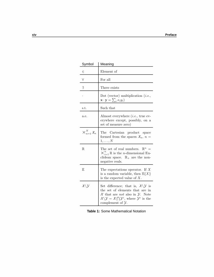
Derivatives of single-variable functions are typically denoted by primes (e.g.,f ′(x) = df(x)/dx). Table 1 summarizes some of the other mathematical nota-tion.
xiii
xiv Preface
Symbol Meaning
∈ Element of
∀ For all
∃ There exists
· Dot (vector) multiplication (i.e.,x · y =
∑i xiyi)
s.t. Such that
a.e. Almost everywhere (i.e., true ev-erywhere except, possibly, on aset of measure zero)
×N
n=1 Xn The Cartesian product spaceformed from the spaces Xn, n =1, . . . , N
R The set of real numbers. Rn =
×n
i=1 R is the n-dimensional Eu-clidean space. R+ are the non-negative reals.
E The expectations operator. If Xis a random variable, then EXis the expected value of X .
X\Y Set difference; that is, X\Y isthe set of elements that are inX that are not also in Y. NoteX\Y = X ⋂Yc, where Yc is thecomplement of Y.
Table 1: Some Mathematical Notation

Pricing
1

Purpose
If one had to distill economics down to a single-sentence description, one prob-ably couldn’t do better than describe economics as the study of how prices areand should be set. This portion of the Lecture Notes is primarily focused onthe normative half of that sentence, how prices should be set, although I hopeit also offers some positive insights as well.
Because I’m less concerned with how prices are set, these notes don’t considerprice setting by the Walrasian auctioneer or other competitive models. Nor is itconcerned with pricing in oligopoly. Our attention will be exclusively on pricingby a single seller who is not constrained by competitive or strategic pressures(e.g., a monopolist).
Now, one common way to price is to set a price, p, per unit of the good inquestion. So, for instance, I might charge $10 per coffee mug. You can buy asmany or as few coffee mugs as you wish at that price. The revenue I receive is$10 times the number of mugs you purchase. Or, more generally, at price p perunit, the revenue from selling x units is px. Because px is the formula for a linethrough the origin with slope p, such pricing is called linear pricing .
If you think about it, you’ll recognize that linear pricing is not the only typeof pricing you see. Generically, pricing in which revenue is not a linear functionof the amount sold is called nonlinear pricing .1 Examples of nonlinear pricingwould be if I gave a 10% discount if you purchased five or mugs (e.g., revenueis $10x if x < 5 and $9x if x ≥ 5). Of if I had a “buy one mug, get one free”promotion (e.g., revenue is $10 if x = 1 or 2, $20 if x = 3 or 4, etc.). Or if I gaveyou a $3-dollar gift with each purchase (e.g., revenue is $10x−3). Alternatively,the price per mug could depend on some other factor (e.g., I offer a weekenddiscount or a senior-citizen discount). Or I could let you have mugs at $5 permug, but only if you buy at least $50 worth of other merchandise from my store.Or I could pack 2 mugs in a box with a coffee maker and not allow you to buymugs separately at all.
1Remember in mathematics a function is linear if αf(x0)+βf(x1) = f(αx0 +βx1), whereα and β are scalars. Note, then, that a linear function from R to R is linear only if it has theform f(x) = Ax.
3

4 Purpose
Buyers and Demand 1A seller sets prices and buyers respond. To understand how they respond, weneed to know what their objectives are. If they are consumers, the standardassumption is that they wish to maximize utility. If they are firms, the pre-sumption is they wish to maximize profits.
Consumer Demand 1.1In the classic approach to deriving demand,1 we maximize an individual’s utilitysubject to a budget constraint; that is,
maxx
u(x)
subject to p · x ≤ I ,(1.1)
where x is an N -dimensional vector of goods, p is the N -dimensional pricevector, and I is income. Solving this problem yields the individual’s demandcurve for each good n, x∗n(pn;p−n, I) (where the subscript −n indicates that it isthe N−1-dimensional subvector of prices other than the price of the nth good).Unfortunately, while this analysis is fine for studying linear pricing, it is hardto utilize for nonlinear pricing: The literature on nonlinear pricing typicallyrequires that the inverse of individual demand also represent the consumer’smarginal benefit curve (i.e., the benefit the consumer derives from a marginalunit of the good).2 Unless there are no income effects, this is not a feature ofdemand curves.
For this reason, we will limit attention to quasi-linear utility . Assume thateach individual j purchases two goods. The amount of the one in which we’reinterested (i.e., the one whose pricing we’re studying) is denoted x. The amountof the other good is denoted y. We can (and will) normalize the price of goody to 1. We can, if we like, consider y to be the amount of consumption otherthan of good x. The utility function is assumed to have the form
u(x, y) = v(x) + y . (1.2)
1As set forth, for instance, in Mas-Colell et al. (1995) or Varian (1992).
2Recall that a demand function is a function from price to quantity; that is, for any givenprice, it tells us the amount the consumer wishes to purchase. Because demand curves slopedown—Giffen goods don’t exist—the demand function is invertible. Its inverse, which is afunction from quantity to price, tells us for any quantity the price at which the consumerwould be willing to purchase exactly that quantity (assuming linear pricing).
5
6 Lecture Note 1: Buyers and Demand
With two goods, we can maximize utility by first solving the constraint in (1.1)for y, yielding y = I − px (recall y’s price is 1), and then substituting that intothe utility function to get an unconstrained maximization problem:3
maxx
v(x) − px+ I . (1.3)
Solving, we have the first-order condition
v′(x) = p . (1.4)
Observe (1.4) also defines the inverse demand curve and, as desired, we havemarginal benefit of x equal to inverse demand. If we define P (x) to be theinverse demand curve, then we have
∫ x
0
P (t)dt =
∫ x
0
v′(t)dt
= v(x) − v(0) .
The second line is the gain in utility—benefit—the consumer obtains from ac-quiring x. Substituting this back into (1.3) we see that utility at the utility-maximizing quantity is equal to
∫ x
0
P (t)dt− xP (x) (1.5)
plus an additive constant, which we are free to ignore. In other words, utility,up to an additive constant, equals the area below the inverse demand curveand above the price of x. See Figure 1.1. You may also recall that (1.5) is theformula for consumer surplus (cs).
Summary 1 Given quasi-linear utility, the individual’s inverse demand curvefor a good is his or her marginal benefit for that good. Moreover, his or herutility at the utility-maximizing quantity equals (to an affine transformation)his or her consumer surplus (i.e., the area below inverse demand and above theprice).
Another way to think about this is to consider the first unit the individualpurchases. It provides him or her (approximate) benefit v′(1) and costs him orher p. His or her surplus or profit is, thus, v′(1) − p. For the second unit thesurplus is v′(2) − p. And so forth. Total surplus from x units, where v′(x) = p,is, therefore,
x∑
t=1
(v′(t) − p) ;
3Well, actually, we need to be careful; there is an implicit constraint that y ≥ 0. In whatfollows, we assume that this constraint doesn’t bind.

1.1 Consumer Demand 7
x
$/unit
units
P(x)
inverse demand
(P(t) = v'(t))
CS
Figure 1.1: Consumer surplus (CS) at quantity x is the area beneath inversedemand curve (P (t)) and above inverse demand at x, P (x).
or, passing to the continuum (i.e., replacing the sum with an integral),
∫ x
0
(v′(t) − p) dt =
∫ x
0
v′(t)dt− px =
∫ x
0
P (t)dt− px .
Yet another way to think about this is to recognize that the consumer wishesto maximize his or her surplus (or profit), which is total benefit, v(x), minushis or her total expenditure (or cost), px. As always, the solution is found byequating marginal benefit, v′(x), to marginal cost, p.
Bibliographic Note
One of the best treatments of the issues involved in measuring consumer surpluscan be found in Chapter 10 of Varian (1992). This is a good place to go to getfull details on the impact that income effects have on measures of consumerwelfare.
Quasi-linear utility allows us to be correct in using consumer surplus as ameasure of consumer welfare. But even if utility is not quasi-linear, the errorfrom using consumer surplus instead of the correct measures, compensating orequivalent variation (see Chapter 10 of Varian), is quite small under assumptionsthat are reasonable for most goods. See Willig (1976). Hence, as a general rule,we can use consumer surplus as a welfare measure even when there’s no reasonto assume quasi-linear utility.

8 Lecture Note 1: Buyers and Demand
Firm Demand 1.2Consider a firm that produces F (x) units of a good using inputs x. Let the factorprices be p and let R(·) be the revenue function. Then the firm maximizes
R(F (x)
)− p · x . (1.6)
The first-order condition with respect to input xn is
R′(F (x)) ∂F∂xn
− pn = 0 . (1.7)
Let x∗[p] denote the set of factor demands, which is found by solving the set ofequations (1.7). Define the profit function as
π(p) = R(F (x∗[p])
)− p · x∗[p] .
Utilizing the envelope theorem, it follows that
∂π
∂pn= −x∗n(pn;p−n) . (1.8)
Consequently, integrating (1.8) with respect to the price of the nth factor, wehave
−∫ ∞
pn
∂π(t;p−n)
∂pndt =
∫ ∞
pn
x∗n(t;p−n)dt . (1.9)
The right-hand side of (1.9) is just the area to the left of the factor demandcurve that’s above price pn. Equivalently, it’s the area below the inverse factordemand curve and above price pn. The left-hand side is π(pn;p−n)−π(∞;p−n).The term π(∞;p−n) is the firm’s profit if it doesn’t use the nth factor (whichcould be zero if production is impossible without the nth factor). Hence, theleft-hand side is the increment in profits that comes from going from beingunable to purchase the nth factor to being able to purchase it at price pn. Thisestablishes
Proposition 1 The area beneath the factor demand curve and above a givenprice for that factor is the total net benefit that a firm enjoys from being able topurchase the factor at that given price.
In other words—as we could with quasi-linear utility—we can use the “con-sumer” surplus that the firm gets from purchasing a factor at a given price asthe value the firm places on having access to that factor at the given price.
Observation 1 One might wonder why we have such a general result with fac-tor demand, but we didn’t with consumer demand. The answer is that withfactor demands there are no income effects. Income effects are what keep con-sumer surplus from capturing the consumer’s net benefit from access to a good atits prevailing price. Quasi-linear utility eliminates income effects, which allowsus to treat consumer surplus as the right measure of value or welfare.
1.3 Demand Aggregation 9
Demand Aggregation 1.3Typically, a seller sells to more than one buyer. For some forms of pricing it isuseful to know total demand as a function of price.
Consider two individuals. If, at a price of $3 per unit, individual one buys4 units and individual two buys 7 units, then total or aggregate demand at $3per unit is 11 units. More generally, if we have J buyers indexed by j, eachof whom has individual demand xj(p) as a function of price, p, then aggregate
demand is∑J
j=1 xj(p) ≡ X(p).How does aggregate consumer surplus (i.e., the area beneath aggregate de-
mand and above price) relate to individual consumer surplus? To answer this,observe that we get the same area under demand and above price whether weintegrate with respect to quantity or price. That is, if x(p) is a demand functionand p(x) is the corresponding inverse demand, then
∫ x
0
(p(t) − p(x)
)dt =
∫ ∞
p
x(t)dt .
Consequently, if CS(p) is aggregate consumer surplus and csj(p) is buyer j’sconsumer surplus, then
CS(p) =
∫ ∞
p
X(t)dt
=
∫ ∞
p
J∑
j=1
xj(t)
dt
=
J∑
j=1
(∫ ∞
p
xj(t)dt
)
=
J∑
j=1
csj(p) ;
that is, we have:
Proposition 2 Aggregate consumer surplus is the sum of individual consumersurplus.
Additional Topics 1.4A Continuum of Consumers
In many modeling situations, it is convenient to imagine a continuum of con-sumers (e.g., think of each consumer having a unique “name,” which is a real
10 Lecture Note 1: Buyers and Demand
number in the interval [0, 1]; and think of all names as being used). Ratherthan thinking of the number of consumers—which would here be uncountablyinfinite—we think about their measure; that is, being rather loose, a functionrelated to the length of the interval.
It might at first seem odd to model consumers as a continuum. One way tothink about it, however, is the following. Suppose there are J consumers. Eachconsumer has demand
x(p) =
1 , if p ≤ v0 , if p > v
, (1.10)
where v is a number, the properties of which will be considered shortly. Thedemand function given by (1.10) is sometimes referred to as L-shaped demandbecause, were one to graph it, the curve would resemble a rotated L.4 Thedemand function also corresponds to the situation in which the consumer wantsat most one unit and is willing to pay up to v for it.
Assume, for each consumer, that v is a random draw from the interval [v0, v1]according to the distribution function F : R → [0, 1]. Assume the draws areindependent. Each consumer knows the realization of his or her v prior tomaking his or her purchase decision.
In this case, each consumer’s expected demand is the probability that he orshe wants the good at the given price; that is, the probability that his or her v ≥p. That probability is 1−F (p) ≡ Σ(p). The function Σ(·) is known in probabilitytheory as the survival function.5 Aggregate expected demand is, therefore,JΣ(p) (recall the consumers’ valuations, v, are independently distributed).
Observe, mathematically, this demand function would be the equivalent ofassuming that there are a continuum of consumers living on the interval [v0, v1],each consumer corresponding to a fixed valuation, v. Assume further that themeasure of consumers on an the interval between v and v′ is JF (v′) − JF (v)or, equivalently, JΣ(v) − JΣ(v′). As before, consumers want at most one unitand they are willing to pay at most their valuation. Interpret demand at p asbeing the measure of consumers in [p, v1]; that is,
JΣ(p) − JΣ(v1) = JΣ(p) ,
where the equality follows because Σ(·) at the end of the support of the func-tion (the right-end of the interval) is zero. In other words, one can view theassumption of a continuum of consumers as being shorthand for a model witha finite number of consumers, each of whom has stochastic demand.
4Note, if one wants to get technical, the curve is really two line segments, one going from(1, 0) to (1, v) (using the usual orientation in which price is on the vertical axis), the othergoing from (0, v) to (0,∞) (the latter interval is open on both ends). If, however, one lookedat only the former interval and drew a horizontal line at the point of discontinuity, then onegets a rotated L.
5The name has an actuarial origin. If the random variable in question is age at death,then Σ(age) is the probability of surviving to at least that age. Admittedly, a more naturalmnemonic for the survival function would be S(·); S(p), however, is “reserved” in economicsfor the supply function.
1.4 Additional Topics 11
A possible objection is that assuming a continuum of consumers on, say,[v0, v1] with aggregate demand JΣ(p) is a deterministic specification, whereasJ consumers with random demand is a stochastic specification. In particular,there is variance in realized demand with the latter, but not the former.6 Inmany contexts, though, this is not important because other assumptions makethe price setter risk neutral.7
Demand as a Survival Function
If demand at zero price, X(0), is finite, and if limp→∞X(p) = 0, then anydemand function is a multiplicative scalar of a survival function; that is,
X(p) = X(0)Σ(p) , (1.11)
where Σ(p) ≡ X(p)/X(0). To see that Σ(·) is a survival function on R+, observethat Σ(0) = 1, limp→∞ Σ(p) = 0, and, because demand curves slope down, Σ(·)in non-decreasing.
Assume Σ(·) is differentiable. Let f(p) = −Σ′(p). The function f(·) is thedensity function associated with the survival function Σ(·) (or, equivalently, withthe distribution function 1 − Σ(p) ≡ F (p)). In demography or actuary science,an important concept is the death rate at a given age, which is the probabilitysomeone that age will die within the year. Treating time continuously, the deathrate can be seen as the instantaneous probability of dying at time t conditionalon having survived to t. (Why conditional? Because you can’t die at time tunless you’ve lived to time t.) The unconditional probability of dying at t isf(t), the probability of surviving to t is Σ(t), hence the death rate is f(t)/Σ(t).Outside of demographic and actuarial circles, the ratio f(t)/Σ(t) is known asthe hazard rate. Let h(t) denote the hazard rate.
In terms of demand, observe
X ′(p)
X(p)=X(0)Σ′(p)
X(0)Σ(p)= −h(p) . (1.12)
In this context, h(p) is the proportion of all units demanded at price p that willvanish if the price is increased by an arbitrarily small amount; that is, it’s thehazard (death) rate of sales that will vanish (die) if the price is increased.
You may recall that the price elasticity of demand, ǫ, is minus one times thepercentage change in demand per a one-percentage-point change in price.8 In
6For example, if, J = 2, [v0, v1] = [0, 1], and F (v) = v on [0, 1] (uniform distribution),then realized demand at p ∈ (0, 1) is 0 with positive probability p2, 1 with positive probability2p(1 − p), and 2 with positive probability (1 − p)2.
7It would be incorrect to appeal to the law of large numbers and act as if J → ∞ meansrealized demand tends to JΣ(p) according to some probability-theoretic convergence criterion.If, however, there is a continuum of consumers with identical and independently distributeddemands, then it can be shown that realized demand is almost surely mean demand (see, e.g.,
Uhlig, 1996).
8Whether one multiplies or not by −1 is a matter of taste; some authors (including thisone on occasion) choose not to.

12 Lecture Note 1: Buyers and Demand
other words
ǫ = −1 ×(
∆X
X× 100%
)÷(
∆p
p× 100%
), (1.13)
where ∆ denotes “change in.” If we pass to the continuum, we see that (1.13)can be reexpressed as
ǫ = −dX(p)
dp× p
X= ph(p) , (1.14)
where the last equality follows from (1.12). In other words, price elasticity placesa monetary value on the proportion of sales lost from a price increase.
Other Relations
For future reference, let’s consider some relations among demand, the associatedhazard rate, and price elasticity. In what follows, we continue to assume X(0)is finite and limp→∞X(p) = 0.
Lemma 1 Σ(p) = exp(−∫ p0h(z)dz
).
Proof:
d log(Σ(p)
)
dz=
−f(p)
Σ(p)
= −h(p) .
Solving the differential equation:
log(Σ(p)
)= −
∫ p
0
h(z)dz + log(Σ(0)
)︸ ︷︷ ︸
=0
.
The result follows by exponentiating both sides.
Immediate corollaries of Lemma 1 are
Corollary 1
(i) There exists a constant ξ such that
X(p) = ξ exp(−∫ p
0
h(z)dz)
= ξ exp(−∫ p
0
ǫ(z)
zdz)
(where ǫ(p) is the price elasticity of demand at price p).
(ii) Suppose X1(p) = ζX2(p) for all p, where Xi(·) are demands and ζ is apositive constant. Let ǫi(·) be the price-elasticity function associated withXi(·). Then ǫ1(p) = ǫ2(p) for all p.
(iii) Suppose ǫ(p) = pkp+p0
, where k and p0 are positive constants. Then X(p) =
ξ(p+ p0)−k. Observe limp0→0 ǫ(p) = k and limp0→0X(p) = ξp−k.
1.4 Additional Topics 13
Exercise: Prove Corollary 1.
Exercise: Why in Corollary 1(iii) was it necessary to assume p0 > 0?
Exercise: Verify by direct calculation (i.e., using the formula ǫ = pX ′(p)/X(p))that a demand function of the form X(p) = ξp−k has a constant elasticity.
Lemma 2 Consumer surplus at price p, CS(p), satisfies
CS(p) = X(0)
∫ ∞
p
(b− p)f(b)db , (1.15)
where f(·) is the density function associated with Σ(·).
Proof: Recall the definition of consumer surplus is area to the left of demandand above price:
CS(p) =
∫ ∞
p
X(b)db
= X(0)
∫ ∞
p
Σ(b)db
= X(0)
(bΣ(b)
∣∣∣∞
p−∫ ∞
p
bΣ′(b)db
)(1.16)
= X(0)
(−p(1 − F (p)
)+
∫ ∞
p
bf(b)db
)(1.17)
= X(0)
∫ ∞
p
(b− p)f(b)db .
Observe (1.16) follows by integration by parts.9 Expression (1.17) follows usingthe relations Σ(p) = 1 − F (p) and Σ′(p) = −f(p).
The integral in (1.15) is an expected value since f(·) is a density. If we thoughtof the benefit enjoyed from each unit of the good as a random variable withdistribution F (·), then the integral in (1.15) is the expected net benefit (surplus)a given unit will yield a consumer (recalling, because he or she need not purchase,that the net benefit function is maxb−p, 0). The amountX(0) can be thoughtof as the total number of units (given that at most X(0) units trade). So theoverall expression can be interpreted as expected (or average) surplus per itemtimes the total number of items.
9To get technical, I’ve slipped in the assumption that limb→∞ bΣ(b) = 0. This is innocuousbecause, otherwise, consumer surplus would be infinite, which is both unrealistic and notinteresting; the latter because, then, welfare would always be maximized (assuming finitecosts) and there would, thus, be little to study.

14 Lecture Note 1: Buyers and Demand
Exercise: Prove that if limb→∞ bX(b) > 0, then consumer surplus at anyprice p is infinite. Hints: Suppose limb→∞ bX(b) = L > 0. Fix an η ∈ (0, L).Show there is a b such that X(b) ≥ L−η
bfor all b ≥ b. Does
∫ ∞
b
L− η
bdb
converge? Show the answer implies∫∞pX(b)db does not converge (i.e., is infi-
nite).
A function, g(·), is log concave if log(g(·))
is a concave function.
Lemma 3 If g(·) is a positive concave function, then it is log concave.10
Proof: If g(·) were twice differentiable, then the result would follow triviallyusing calculus (Exercise: do such a proof). More generally, let x0 and x1 betwo points in the domain of g(·) and define xλ = λx0+(1−λ)x1. The conclusionfollows, by the definition of concavity, if we can show
log(g(xλ)
)≥ λ log
(g(x0)
)+ (1 − λ) log
(g(x1)
)(1.18)
for all λ ∈ [0, 1]. Because log(·) is order preserving, (1.18) will hold if
g(xλ) ≥ g(x0)λg(x1)
1−λ . (1.19)
Because g(·) is concave by assumption,
g(xλ) ≥ λg(x0) + (1 − λ)g(x1) .
Expression (1.19) will, therefore, hold if
λg(x0) + (1 − λ)g(x1) ≥ g(x0)λg(x1)
1−λ . (1.20)
Expression (1.20) follows from Polya’s generalization of the arithmetic mean-geometric mean inequality (see, e.g., Steele, 2004, Chapter 2),11 which states
10A stronger result can be established, namely that r`
s(·)´
is concave if both r(·) and s(·)are concave and r(·) is non-decreasing. This requires more work than is warranted given whatwe need.
11Polya’s generalization is readily proved. Define A ≡Pn
i=1 λiai. Observe that x + 1 ≤ ex
(the former is tangent to the latter at x = 0 and the latter is convex). Hence, aiA
≤ eaiA
−1.
Because both sides are positive,` ai
A
´λi ≤ eλiai
A−λi . We therefore have
Y
i=1n
“ ai
A
”λi ≤Y
i=1n
eλiai
A−λi
= ePn
i
“
λiaiA
−λi
”
.
The last term simplifies to 1, so we have
Q
i=1n aλii
AP
ni=1
λi≤ 1 .
Because the denominator on the left is just A, the result follows.

1.4 Additional Topics 15
that if a1, . . . , an ∈ R+, λ1, . . . , λn ∈ [0, 1], and∑n
i=1 λi = 1, then
n∑
i=1
λiai ≥n∏
i=1
aλi
i . (1.21)
Observe the converse of Lemma 3 need not hold. For instance, x2 is log concave(2 log(x) is clearly concave in x), but x2 is not itself concave. In other words, log-concavity is a weaker requirement than concavity. As we will see, log concavityis often all we need for our analysis, so we gain a measure of generality byassuming log-concavity rather than concavity.
The hazard rate is monotone if it is either everywhere non-increasing oreverywhere non-decreasing. The latter case is typically the more relevant (e.g.,the death rate for adults increases with age) and is a property of many familiardistributions (e.g., the uniform, the normal, the logistic, among others). Whena hazard rate is non-decreasing, we say it satisfies the monotone hazard rateproperty . This is sometimes abbreviated as mhrp.
Lemma 4 A demand function is (strictly) log concave if and only if the corre-sponding hazard rate satisfies the (strict) monotone hazard rate property.
Proof: It is sufficient for X(·) to be log concave that the first derivative oflog(X(·)
)—that is,
d log(X(p)
)
dp=X ′(p)
X(p)= −h(p)
—be non-increasing (decreasing) in p. Clearly it will be if h(·) is non-decreasing(increasing). To prove necessity, assume X(·) is (strictly) log concave, then−h(·) must be non-increasing (decreasing), which is to say that h(·) is non-decreasing (increasing).
Lemma 5 If demand is log concave, then so to is consumer expenditure underlinear pricing; that is, X(·) log concave implies pX(p) is log concave for all p.
Proof: Given that log(pX(p)
)≡ log(p) + log
(X(p)
), the first derivative of
log(pX(p)
)is
1
p+X ′(p)
X(p).
The first term is clearly decreasing in p and the second term is decreasing in pby assumption.
Exercise: Suppose the hazard rate is a constant. Prove that pX(p) is, there-fore, everywhere strictly log concave.

16 Lecture Note 1: Buyers and Demand
Exercise: Prove that linear (affine) demand (e.g., X(p) = a − bp, a and bpositive constants) is log concave.
Exercise: Prove that if demand is log concave, then elasticity is increasing inprice (i.e., ǫ(·) is an increasing function).
Exercise: Prove that if price elasticity is increasing in price, then consumerexpenditure is log concave; that is, show ǫ(·) increasing implies pX(p) is logconcave for all p.
Linear Pricing 2In this section, we consider a firm that sells all units at a constant price perunit. If p is that price and it sells x units, then its revenue is px. Such linearpricing is also called simple monopoly pricing .
Assume this firm incurs a cost of C(x) to produce x units. Suppose, too, thatthe aggregate demand for its product is X(p) and let P (x) be the correspondinginverse demand function. Hence, the maximum price at which it can sell x unitsis P (x), which generates revenue xP (x). LetR(x) denote the firm’s revenue fromselling x units; that is, R(x) = xP (x). The firm’s profit is revenue minus cost,R(x) − C(x). The profit-maximizing amount to sell maximizes this difference.
If we assume
∃x ∈ [0,∞) such that R(x) − C(x) ≤ 0 ∀x > x (lp)
and
∀x0 ∈ R+ , x→ x0 ⇒ R(x) − C(x) → R(x0) − C(x0) (continuity) , (lp)
then there must exist at least one profit-maximizing quantity.If we strengthen (lp) by assuming
R(·) and C(·) are differentiable , (lp′)
then
R′(x) − C′(x) = 0 (2.1)
if x is profit maximizing; or, as it is sometimes written,
MR(x) = MC (x)
where MR denotes marginal revenue and MC denotes marginal cost.In many applications, we would like (2.1) to be sufficient as well as necessary.
For (2.1) to be sufficient, the maximum cannot occur at a corner. To rule out acorner solution assume
∃x ∈ R+ such that R(x) − C(x) > 0 . (lp)
This expression says that positive profit is possible. Given that profit at the“corners,” 0 and x, is zero, this rules out a corner solution. That profit at x is
17

18 Lecture Note 2: Linear Pricing
zero follows by assumptions (lp) and (lp). That profit at 0 is zero followsbecause C(0) ≡ 0 (if one is not doing an activity, then one is not forgoinganything to do it) and there can be no revenue from selling nothing.
For (2.1) to be sufficient it must also be true that it does not define aminimum (or an inflection point) and that there not be more than one localmaximum. The following propositions provide conditions sufficient to ensurethose conditions are met. Both propositions make use of the fact that
MR(x) = P (x) + xP ′(x) . (2.2)
Proposition 3 Maintain assumptions lp, lp′, and lp. Assume demand,X(·), is log concave and cost, C(·), is at least weakly convex, then MR(x) =MC(x) is sufficient as well as necessary for the profit-maximizing quantity.
Proof: Because an interior maximum exists, we know that (2.1) must holdfor at least one x. If it holds for only one x, then that x must be the global
maximum. Using the fact that ǫ = − P (x)xP ′(X) and expression (2.2), we can write
(2.1) as
P (x)
(1 − 1
ǫ
)− C′(x) = 0 . (2.3)
Solving (2.3) for 1/ǫ and making the substitutions p = P(X(p)
)and x = X(p),
we have1
ǫ(p)=p− C′(X(p)
)
p. (2.4)
(For future reference, note that expression (2.4) is known as the Lerner markuprule.) We are done if we can show that only one p can solve (2.4). As noted,at least one p must solve (2.4). If the left-hand side of (2.4) is decreasing in pand the right-hand side increasing, then the p that solves (2.4) must be unique.Because X(·) is log concave, price elasticity of demand, ǫ(·), is increasing (seethe exercises following Lemma 5); hence, 1/ǫ(p) is decreasing in p. To show theright-hand side of (2.4) is increasing consider p and p′, p > p′. It is readily seenthat (2.4) is greater evaluated at p rather than p′ if
C′(X(p))
p<C′(X(p′)
)
p′.
Given p′ < p, that will be true if C′(X(p))≤ C′(X(p′)
). Because demand
curves are non-increasing, X(p) ≤ X(p′). Because C(·) weakly convex impliesC′(·) is non-decreasing, the result follows.
Proposition 4 Maintain assumptions lp, lp′, and lp. Suppose (i) demandslopes down (P ′(·) < 0); (ii) inverse demand is log concave; (iii) inverse demandand cost are at least twice differentiable; and (iv) P ′(x) < C′′(y) for all x andall y ∈ [0, x] (i.e., cost is never “too concave”). Then MR(x) = MC(x) issufficient as well as necessary for the profit-maximizing quantity.

2.1 Elasticity and the Lerner Markup Rule 19
Proof: Consider an x such that MR(x) = MC(x) (at least one exists becausethere is an interior maximum). In other words, consider an x such that
xP ′(x) + P (x) − C′(x) = 0 . (2.5)
If the derivative of (2.5) is always negative evaluated at any x that solves (2.5),then that x is a maximum. Moreover, it is the unique maximum because a func-tion cannot have multiple (local) maxima without minima; and if the derivativeof (2.5) is always negative at any x that solves (2.5), then R(x) − C(x) hasno interior minima (recall (2.5) is also a necessary condition for x to minimizeR(x) − C(x)). Differentiating (2.5) yields
2P ′(x) + xP ′′(x) − C′′(x) = xP ′′(x) + P ′(x) + P ′(x) − C′′(x)︸ ︷︷ ︸<0
.
It follows we’re done if xP ′′(x) + P ′(x) ≤ 0. Given that demand curves slopedown, we’re done if P ′′(x) ≤ 0. Suppose, therefore, that P ′′(x) > 0. Theassumption that P (·) is log concave implies
P (x)P ′′(x) −(P ′(x)
)2 ≤ 0 . (2.6)
Because cost is non-decreasing, (2.5) implies P (x) ≥ −P ′(x)x. So (2.6) implies
0 ≥ −P ′(x)xP ′′(x) −(P ′(x)
)2 ⇒ 0 ≥ xP ′′(x) + P ′(x) (2.7)
(recall −P ′(x) > 0).
Because demand curves slope down, P ′(x) < 0; hence, expression (2.2) im-plies MR(x) < P (x), except at x = 0 where MR(0) = P (0). See Figure 2.1.Why is MR(x) < P (x)? That answer is that, to sell an additional item, thefirm must lower its price (i.e., recall, P (x + ε) < P (x), ε > 0). So marginalrevenue has two components: The price received on the marginal unit, P (x),less the revenue lost on the infra-marginal units from having to lower the price,|xP ′(x)| (i.e., the firm gets |P ′(x)| less on each of the x infra-marginal units).
Elasticity and the LernerMarkup Rule 2.1
We know that the revenue from selling 0 units is 0. For “sensible” demandcurves, limx→∞ xP (x) = 0 because eventually price is driven down to zero.In between these extremes, revenue is positive. Hence, we know that revenuemust increase over some range of output and decrease over another. Revenue isincreasing if and only if
P (x) + xP ′(x) > 0 or xP ′(x) > −P (x) .

20 Lecture Note 2: Linear Pricing
$/unit
units
inverse demand
(P(x))
MR
MC
xM*
P( )xM*
Figure 2.1: Relation between inverse demand, P (x), and marginal revenue,MR, under linear pricing; and the determination of the profit-maximizing quantity, x∗M , and price, P (x∗M ).
Divide both sides by −P (x) to get
1 > −xP′(x)
P (x)=
1
ǫ. (2.8)
Multiplying both sides of (2.8) by ǫ, we have that revenue is increasing if andonly if
ǫ > 1 . (2.9)
When ǫ satisfies (2.9), we say that demand is elastic. When demand is elastic,revenue is increasing with units sold. If ǫ < 1, we say that demand is inelastic.Reversing the various inequalities, it follows that, when demand is inelastic,revenue is decreasing with units sold. The case where ǫ = 1 is called unitelasticity .
Recall that a firm produces the number of units that equates MR to MC .The latter is positive, which means that a profit-maximizing firm engaged inlinear pricing operates only on the elastic portion of its demand curve. Thismakes intuitive sense: If it were on the inelastic portion, then, were it to produceless, it would both raise revenue and lower cost; that is, increase profits. Hence,it can’t maximize profits operating on the inelastic portion of demand.
Summary 2 A profit-maximizing firm engaged in linear pricing operates onthe elastic portion of its demand curve.
2.2 Welfare Analysis 21
Rewrite the MR(x) = MC (x) condition as
P (x) − MC (x) = −xP ′(x)
and divide both sides by P (x) to obtain
P (x) − MC (x)
P (x)= −xP
′(x)
P (x)=
1
ǫ, (2.10)
Expression (2.10) is known as the Lerner markup rule.1 In English, it says thatthe price markup over marginal cost, P (x)−MC (x), as a proportion of the priceis equal to 1/ǫ. Hence, the less elastic is demand (i.e., as ǫ decreases towards 1),the greater the percentage of the price that is a markup over cost. Obviously,the portion of the price that is a markup over cost can’t be greater than theprice itself, which again shows that the firm must operate on the elastic portionof demand.
Welfare Analysis 2.2Assuming that consumer surplus is the right measure of consumer welfare (e.g.,consumers have quasi-linear utility), then total welfare is the sum of firm profitsand consumer surplus. Hence, total welfare is
xP (x) − C(x)︸ ︷︷ ︸profit
+
∫ x
0
(P (t) − P (x))dt
︸ ︷︷ ︸CS
= xP (x) − C(x) +
∫ x
0
P (t)dt− xP (x)
=
∫ x
0
P (t)dt− C(x) . (2.11)
Observe, first, that neither the firm’s revenue, xP (x), nor the consumers’ expen-diture, xP (x), appear in (2.11). This is the usual rule that monetary transfersmade among agents are irrelevant to the amount of total welfare. Welfare isdetermined by the allocation of the real good; that is, the benefit,
∫P (t)dt,
that consumers obtain and the cost, C(x), that the producer incurs.
Next observe that the derivative of (2.11) is P (x) − MC (x). From (2.5) onpage 19 (i.e., from MR(x∗M ) = MC (x∗M )), recall that P (x∗M ) > MC (x∗M ), wherex∗M is the profit-maximizing quantity produced under linear pricing. This meansthat linear pricing leads to too little output from the perspective of maximizingwelfare—if the firm produced more, welfare would increase.
Proposition 5 Under linear pricing, the monopolist produces too little outputfrom the perspective of total welfare.
1Named for the economist Abba Lerner.
22 Lecture Note 2: Linear Pricing
$/unit
units
inverse demand
(P(x))MR
MC
xM*
P( )xM*
xW*
deadweight
loss
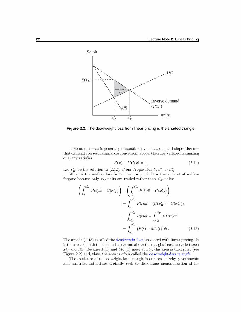
Figure 2.2: The deadweight loss from linear pricing is the shaded triangle.
If we assume—as is generally reasonable given that demand slopes down—that demand crosses marginal cost once from above, then the welfare-maximizingquantity satisfies
P (x) − MC (x) = 0 . (2.12)
Let x∗W be the solution to (2.12). From Proposition 5, x∗W > x∗M .What is the welfare loss from linear pricing? It is the amount of welfare
forgone because only x∗M units are traded rather than x∗W units:
(∫ x∗
W
0
P (t)dt− C(x∗W )
)−(∫ x∗
M
0
P (t)dt− C(x∗M )
)
=
∫ x∗
W
x∗
M
P (t)dt− (C(x∗W ) − C(x∗M ))
=
∫ x∗
W
x∗
M
P (t)dt−∫ x∗
W
x∗
M
MC (t)dt
=
∫ x∗
W
x∗
M
(P (t) − MC (t)
)dt . (2.13)
The area in (2.13) is called the deadweight loss associated with linear pricing. Itis the area beneath the demand curve and above the marginal cost curve betweenx∗M and x∗W . Because P (x) and MC (x) meet at x∗W , this area is triangular (seeFigure 2.2) and, thus, the area is often called the deadweight-loss triangle.
The existence of a deadweight-loss triangle is one reason why governmentsand antitrust authorities typically seek to discourage monopolization of in-

2.3 An Application 23
dustries and, instead, seek to encourage competition. Competition tends todrive price toward marginal cost, which causes output to approach the welfare-maximizing quantity.2
We can consider the welfare loss associated with linear pricing as a motive tochange the industry structure (i.e., encourage competition). We—or the firm—can also consider it as encouragement to change the method of pricing. Thedeadweight loss is, in a sense, money left on the table. As we will see, in somecircumstances, clever pricing by the firm will allow it to pick some, if not all, ofthis money up off the table.
An Example
To help make all this more concrete, consider the following example. A monopolyhas cost function C(x) = 2x; that is, MC = 2. It faces inverse demandP (x) = 100 − x.
Marginal revenue under linear pricing is P (x) + xP ′(x), which equals 100−x + x × (−1) = 100 − 2x.3 Equating MR with MC yields 100 − 2x = 2;hence, x∗M = 49. The profit-maximizing price is 100 − 49 = 51.4 Profit isrevenue minus cost; that is, 51 × 49 − 2 × 49 = 2401.5 Consumer surplus is∫ 49
0(100 − t− 51)dt = 1
2 × 492.6
Total welfare, however, is maximized by equating price and marginal cost:P (x) = 100 − x = 2 = MC . So x∗W = 98. Deadweight loss is, thus,
∫ 98
49
(100 − t︸ ︷︷ ︸P (x)
− 2︸︷︷︸MC
)dt = 98t− 1
2t2∣∣∣∣98
49
= 1200.5 .
As an exercise, derive the general condition for deadweight loss for affine de-mand and constant marginal cost (i.e., under the assumptions of footnote 4).
An Application 2.3We often find simple monopoly pricing in situations that don’t immediately ap-pear to be linear-pricing situations. For example, suppose that a risk-neutral
2A full welfare comparison of competition versus monopoly is beyond the scope of thesenotes. See, for instance, Chapters 13 and 14 of Varian (1992) for a more complete treatment.
3Exercise: Prove that if inverse demand is an affine function, then marginal revenue isalso affine with a slope that is twice as steep as inverse demand.
4Exercise: Prove that, if inverse demand is P (x) = a− bx and MC = c, a constant, thenx∗
M = a−c2b
and P (x∗M ) = a+c
2.
5Exercise: Prove that profit under linear pricing is 1b
`
a−c2
´2under the assumptions of
footnote 4.
6Exercise: Prove that consumer surplus under linear pricing is(a−c)2
8bunder the assump-
tions of footnote 4.
24 Lecture Note 2: Linear Pricing
seller faces a single buyer. Let the seller have single item to sell (e.g., an art-work). Let the buyer’s value for this artwork be v. The buyer knows v, butthe seller does not. All the seller knows is that v is distributed according tothe differential distribution function F (·). That is, the probability that v ≤ vis F (v). Assume F ′(·) > 0 on the support of v. Let the seller’s value for thegood—her cost—be c. Assume F (c) < 1.
Suppose that the seller wishes to maximize her expected profit. Suppose, too,that she makes a take-it-or-leave-it offer to the buyer; that is, the seller quotesa price, p, at which the buyer can purchase the good if he wishes. If he doesn’twish to purchase at that price, he walks away and there is no trade. Clearly, thebuyer buys if and only if p ≤ v; hence, the probability of a sale, x, is given by theformula x = 1 − F (p). The use of “x” is intentional—we can think of x as the(expected) quantity sold at price p. Note, too, that, because the formula x =1−F (p) relates quantity sold to price charged, it is a demand curve. Moreover,because the probability that the buyer’s value is less than p is increasing in p,this demand curve slopes down. Writing F (p) = 1 − x and inverting F (whichwe can do because it’s monotonic), we have p = F−1(1−x) ≡ P (x). The seller’s(expected) cost is cx, so marginal cost is c. The seller’s (expected) revenue isxP (x). As is clear, we have a standard linear-pricing problem. Marginal revenueis
P (x) + xP ′(x) = F−1(1 − x) + x
( −1
F ′[F−1(1 − x)]
).
For example, if c = 1/2 and v is distributed uniformly on [0, 1], then F (v) =v, F ′(v) = 1, and F−1(y) = y. So MR(x) is 1 − 2x. Hence, x∗M = 1/4 and,thus, the price the seller should ask to maximize her expected profit is 3/4.7
Note that there is a deadweight loss: Efficiency requires that the good changehands whenever v > c; that is, in this example, when v > 1/2. But given linearpricing, the good only changes hands when v > 3/4—in other words, half thetime the good should change hands it doesn’t.
7An alternative approach, which is somewhat more straightforward in this context, is tosolve maxp(p − c)
`
1 − F (p)´
.

First-degree PriceDiscrimination 3
We saw in Section 2.2 that linear pricing “leaves money on the table,” in thesense that there are gains to trade—the deadweight loss—that are not realized.There is money to be made if the number of units traded can be increased fromx∗M to x∗W .
Why has this money been left on the table? The answer is that trade benefitsboth buyer and seller. The seller profits to the extent that the revenue receivedexceeds cost and the buyer profits to the extent that the benefit enjoyed ex-ceeds the cost. The seller, however, does not consider the positive externalityshe creates for the buyer (buyers) by selling him (them) goods. The fact thathis (their) marginal benefit schedule (i.e., inverse demand) lies above his (their)marginal cost (i.e., the price the seller charges) is irrelevant to the seller insofaras she doesn’t capture any of this gain enjoyed by the buyer (buyers). Conse-quently, she underprovides the good. This is the usual problem with positiveexternalities: The decision maker doesn’t internalize the benefits others derivefrom her action, so she does too little of it from a social perspective. In contrast,were the action decided by a social planner seeking to maximize social welfare,then more of the action would be taken because the social planner does considerthe externalities created. The cure to the positive externalities problem is tochange the decision maker’s incentives so she effectively faces a decision problemthat replicates the social planner’s problem.
One way to make the seller internalize the externality is to give her thesocial benefit of each unit sold. Recall the marginal benefit of the the xth unitis P (x). So let the seller get P (1) if she sells one unit, P (1) + P (2) if she sellstwo, P (1) +P (2) +P (3) if she sells three, and so forth. Given that her revenuefrom x units is
∫ x0P (t)dt, her marginal revenue schedule is P (x). Equating
marginal revenue to marginal cost, she produces x∗W , the welfare-maximizingquantity.
In general, allowing the seller to vary price unit by unit, so as to marchdown the demand curve, is impractical. But, as we will see, there are ways forthe seller to effectively duplicate marching down the demand curve. When theseller can march down the demand curve or otherwise capture all the surplus,she’s said to be engaging in first-degree price discrimination. This is sometimescalled perfect price discrimination.
25
26 Lecture Note 3: First-degree Price Discrimination
Two-Part Tariffs 3.1Consider a seller who faces a single buyer with inverse demand p(x). Let theseller offer a two-part tariff : The buyer pays as follows:
T (x) =
0 , if x = 0px+ f if x > 0
, (3.1)
where p is price per unit and f is the entry fee, the amount the buyer mustpay to have access to any units. The scheme in (3.1) is called a two-part tariffbecause there are two parts to what the buyer pays (the tariff), the unit priceand the entry fee.
The buyer will buy only if f is not set so high that he loses all his consumersurplus. That is, he buys provided
f ≤∫ x
0
(p(t) − p(x))dt =
∫ x
0
p(t)dt− xp(x) . (3.2)
Constraints like (3.2) are known as participation constraints or individual-rationality ( ir) constraints. These constraints often arise in pricing schemesor other mechanism design. They reflect that, because participation in thescheme or mechanism is voluntary, it must be induced.
The seller’s problem is to choose x (effectively, p) and f to maximize profitsubject to (3.2); that is, maximize
f + xp(x) − C(x) (3.3)
subject to (3.2). Observe that (3.2) must bind: If it didn’t, then the seller couldraise f slightly, keeping x fixed, thereby increasing her profits without violatingthe constraint. Note this means that the entry fee is set equal to the consumersurplus that the consumer receives. Because (3.2) is binding, we can substituteit into (3.3) to obtain the unconstrained problem:
maxx
∫ x
0
p(t)dt− xp(x) + xp(x) − C(x) .
The first-order condition is p(x) = MC (x); that is, the profit-maximizing quan-tity is the welfare-maximizing quantity. The unit price is p(x∗W ) and the entry
fee is∫ x∗
W
0p(t)dt− x∗W p(x
∗W ).
Proposition 6 A seller who sells to a single buyer with known demand doesbest to offer a two-part tariff with the unit price set to equate demand andmarginal cost and the entry fee set equal to the buyer’s consumer surplus at thatunit price. Moreover, this solution maximizes welfare.
Of course, a seller rarely faces a single buyer. If, however, the buyers allhave the same demand, then a two-part tariff will also achieve efficiency and
3.1 Two-Part Tariffs 27
allow the seller to achieve the maximum possible profits. Let there be J buyersall of whom are assumed to have the same demand curve. As before, let P (·)denote aggregate inverse demand. The seller’s problem in designing the optimaltwo-part tariff is
maxf,x
Jf + xP (x) − C(x) (3.4)
subject to consumer participation,
f ≤ csj(P (x)
), (3.5)
where csj(p) denotes the jth buyer’s consumer surplus at price p. Because thebuyers are assumed to have identical demand, the subscript j is superfluousand constraint (3.5) is either satisfied for all buyers or it is satisfied for nobuyer. As before, (3.5) must bind, otherwise the seller could profitably raise f .Substituting the constraint into (3.4), we have
maxx
J × cs(P (x)
)+ xP (x) − C(x) ,
which, because aggregate consumer surplus is the sum of the individual surpluses(recall Proposition 2 on page 9), can be rewritten as
maxx
∫ x
0
P (t)dt− xP (x)
︸ ︷︷ ︸aggregate CS
+xP (x) − C(x) .
The solution is x∗W . Hence, the unit price is P (x∗W ) and the entry fee, f , is
1
J
(∫ x∗
W
0
P (t)dt− x∗WP (x∗W )
).
Proposition 7 A seller who sells to J buyers, all with identical demands, doesbest to offer a two-part tariff with the unit price set to equate demand andmarginal cost and the entry fee set equal to 1/Jth of aggregate consumer surplusat that unit price. This maximizes social welfare and allows the seller to captureall of social welfare.
We see many examples of two-part tariffs in real life. A classic example isan amusement park that charges an entry fee and a per-ride price (the latter,sometimes, being set to zero). Another example is a price for a machine (e.g.,a Polaroid instant camera or a punchcard sorting machine), which is a form ofentry fee, and a price for an essential input (e.g., instant film or punchcards),which is a form of per-unit price.1 Because, in many instances, the per-unit price
1Such schemes can also be seen as a way of providing consumer credit: The price of thecapital good (e.g., camera or machine) is set lower than the profit-maximizing price (absentliquidity constraints), with the difference being essentially a loan to the consumer that herepays by paying more than the profit-maximizing price (absent a repayment motive) for theancillary good (e.g., film or punchcards).
28 Lecture Note 3: First-degree Price Discrimination
is set to zero, some two-part tariffs might not be immediately obvious (e.g., anannual service fee that allows unlimited “free” service calls, a telephone callingplan in which the user pays so much per month for unlimited “free” phone calls,or amusement park that allows unlimited rides with paid admission).
Packaging is another way to design a two-part tariff. For instance, a groceryPackaging: Adisguised two-parttariff. story could create a two-part tariff in the following way. Suppose that, rather
than being sold in packages, sugar were kept in a large bin and customers couldpurchase as much or as little as they liked (e.g., like fruit at most groceries or asis actually done at “natural” groceries). Suppose that, under the optimal two-part tariff, each consumer would buy x pounds, which would yield him surplusof cs, which would be captured by the store using an entry fee of f = cs.Alternatively, but equivalently, the grocery could package sugar. Each bag ofsugar would have x pounds and would cost px + cs per bag. Each consumerwould face the binary decision of whether to buy 0 pounds or x pounds. Eachconsumer’s total benefit from x pounds is px+ cs, so each would just be willingto pay px+ cs for the package of sugar. Because the entry fee is paid on everyx-pound bag, the grocery has devised a (disguised) two-part tariff that is alsoarbitrage-proof. In other words, packaging—taking away consumers ability tobuy as much or as little as they wish—can represent an arbitrage-proof way ofemploying a two-part tariff.
The Two-Instruments Principle
When the seller was limited to just one price parameter, p—that is, engaged inlinear pricing—she made less money than when she controlled two parameters,p and f . One way to explain this is that a two-part tariff allows the seller toface the social planner’s problem of maximizing welfare and, moreover, captureall welfare. Because society can do no better than maximize welfare and theseller can do no better than capture all of social welfare, she can’t do betterthan a two-part tariff in this context.
But this begs the question of why she couldn’t do as well with a single priceparameter. Certainly, she could have maximized social welfare; all she neededto do was set P (x) = MC (x). But the problem with that solution is there isno way for her to capture all the surplus she generates. If she had an entry fee,then she could use this to capture the surplus; but with linear pricing we’veforbidden her that instrument.
The problem with using just the unit price is that we’re asking one instru-ment to do two jobs. One is to determine allocation. The other is to capturesurplus for the seller. Only the first has anything to do with efficiency, so thefact that the seller uses it for a second purpose is clearly going to lead to adistortion. If we give the seller a second instrument, the entry fee, then she hastwo instruments for the two jobs and she can “allocate” each job an instrument.This is a fairly general idea—efficiency is improved by giving the mechanismdesigner more instruments—call this the two-instruments principle.

3.1 Two-Part Tariffs 29
x
y
I
Y(x)
y-
f
x*
Figure 3.1: A general analysis of a two-part tariff.
Two-Part Tariffs without Apology
It might seem that the analysis of two-part tariffs is dependent on our assump-tion of quasi-linear utility. In fact, this is not the case. To see this, consider asingle consumer with utility u(x, y). Normalize the price of y to 1. Assume theindividual has income I. Define Y (x) to be the indifference curve that passesthrough the bundle (0, I); that is, the bundle in which the consumer purchasesonly the y-good. See Figure 3.1. Assume MC = c.
Consider the seller of the x good. If she imposes a two-part tariff, then she transforms the consumer’s budget constraint to be the union of the vertical linesegment (0, y)|I − f ≤ y ≤ I and the line y = (I − f) − px, x > 0. If wedefine y = I − f , then this budget constraint is the thick dark curve shownin Figure 3.1. Given that the consumer can always opt to purchase none ofthe x good, the consumer can’t be put below the indifference curve through(0, I); that is, below Y (x). For a given p, the seller increases profit by raisingf , the entry fee. Hence, the seller’s goal is to set f so that this kinked budgetconstraint is just tangent to the indifference Y (x). This condition is illustratedin Figure 3.1, where the kinked budget constraint and Y (x) are tangent at x∗.If the curves are tangent at x∗, then
−p = Y ′(x∗) . (3.6)
At x∗, the firm’s profit is(p− c)x∗ + f (3.7)
(recall we’ve assumed MC = c). As illustrated, f = I − y. In turn, y =

30 Lecture Note 3: First-degree Price Discrimination
Y (x∗) + px∗.2 We can, thus, rewrite (3.7) as
(p− c)x∗ + I − Y (x∗) − px∗ = −Y (x∗) − cx∗ + I . (3.8)
Maximizing (3.8) with respect to x∗, we find that c = −Y ′(x∗). Substituting forY ′(x∗) using (3.6), we find that c = p; that is, as before, the seller maximizesprofits by setting the unit price equal to marginal cost. The entry fee is I −(Y (x∗) + cx∗), where x∗ solves c = −Y ′(x∗). Given that MC = c, it is clearthis generalizes for multiple consumers.
Summary 3 The conclusion that the optimal two-part tariff with one consumeror homogeneous consumers entails setting the unit price equal to marginal costis not dependent on the assumption of quasi-linear utility.
As a “check” on this analysis, observe that Y ′(·) is the marginal rate ofsubstitution (mrs). With quasi-linear utility; that is, u(x, y) = v(x)+y, the mrs
is −v′(x). So x∗ satisfies c = −(−v′(x)) = v′(x) = P (x), where the last equalityfollows because, with quasi-linear utility, the consumer’s inverse demand curveis just his marginal benefit (utility) of the good in question. This, of course,corresponds to what we found above (recall Proposition 6).
Bibliographic Note
For more on two-part and multi-part tariffs, see Wilson (1993). Among othertopics, Wilson investigates optimal two-part tariffs with heterogeneous con-sumers. Varian (1989) is also a useful reference.
2Because the line segment y − px is tangent to Y (·) at x∗, we have y − px∗ = Y (x∗).

Third-degree PriceDiscrimination 1 4
In real life, consumers are rarely homogenous with respect to their preferencesand, hence, demands. We wish, therefore, to extend our analysis of price dis-crimination to accommodate heterogenous consumers.
The Notion of Type 4.1To analyze heterogeneous consumers, imagine that we can index the consumers’different utility functions, which here is equivalent to indexing their differentdemand functions. We refer to this index as the type space, a given type beinga specific index number. All consumers of the same type have the same demand.For example, suppose all consumers have demand of the form
x(p) =
1 , if p ≤ θ0 , if p > θ
;
that is, a given consumer wants at most one unit and only if price does notexceed θ. Suppose θ varies across consumers. In this context, θ is a consumer’stype (index). The set of possible values that θ can take is the type space. Forinstance, suppose that consumers come in one of two types, θ = 10 or θ = 15.In this case, the type space, Θ, can be written as Θ = 10, 15. Alternatively,we could have a continuous type space; for instance, Θ = [a, b], a and b ∈ R+.
Consider the second example. Suppose there is a continuum of consumersof measure J whose types are distributed uniformly over [a, b]. Consequently,at a uniform price of p, demand is J b−p
b−a . Suppose the firm’s cost of x units iscx; observe MC = c. As there would otherwise be no trade, assume c < b. Ifthe firm engaged in linear pricing, its profit-maximizing price would be
p∗ =
b+c2 , if b+c
2 ≥ a
a , if b+c2 < a
.
(Exercise: Verify.) Rather than deal with both cases, assume a < (b + c)/2.Given this last assumption, there is no further loss of generality in normalizingthe parameters so a = 0, b = 1, and 0 ≤ c < 1.
1What happened to second-degree price discrimination? Despite the conventional ordering,it makes more sense to cover third-degree price discrimination before second-degree pricediscrimination.
31

32 Lecture Note 4: Third-degree Price Discrimination
The firm’s profit is
πLP = J(1 − c)2
4. (4.1)
(Exercise: Verify.)Suppose, instead of linear pricing, the firm knew each consumer’s type and
could base its price to that consumer on his type. Because a consumer is willingto pay up to θ, the firm maximizes its profit by charging each consumer θ(provided θ ≥ c). Given that the firm is capturing all the surplus, this is perfectdiscrimination. The firm’s profit is
πPD = J
∫ 1
c
(θ − c)dθ = J(1 − c)2
2. (4.2)
Clearly, this exceeds the profit given in (4.1). Of course, we knew this wouldbe the case without calculating (4.2): linear pricing, because it generates adeadweight loss and leaves some surplus in consumer hands, cannot yield thefirm as great a profit as perfect discrimination.
The example illustrates that, with heterogenous consumers, the ideal fromthe firm’s perspective would be to base its prices on consumers’ types. In mostsettings, however, that is infeasible. The question then becomes how closely canthe firm approximate that ideal through its pricing.
Characteristic-basedDiscrimination 4.2
When a seller cannot observe consumers’ types, she has two choices. One, shecan essentially ask consumers their type; this, as we will see in the next chapter,is what second-degree price discrimination is all about. Two, she can baseher prices on observable characteristics of the consumers, where the observablecharacteristics are correlated in some way with the underlying types. This isthird-degree price discrimination.
Examples of third-degree price discrimination are pricing based on observ-able characteristics such as age, gender, student status, geographic location, ortemporally different markets.2 The idea is that, say, student status is correlatedwith willingness to pay; on average, students have a lower willingness to pay foran event (e.g., a movie) than do working adults.
Formally, consider a seller who can discriminate on the basis of M observabledifferences. Let m denote a particular characteristic (e.g., m = 1 is student andm = 2 = M is other adult). Based on the distribution of types conditional onm, the firm’s demand from those with characteristic m is Xm(·). Let Pm(·) bethe corresponding inverse demand. For example, suppose individual demandis the L-shaped demand of the previous section, θ|m = 1 ∼ 1 − (1 − θ)2 on[0, 1], and θ|m=2 ∼ θ2 (observe the second dominates the first in the sense of
2Although pricing differently at different times could also be part of second-degree pricediscrimination scheme.
4.3 Welfare Considerations 33
first-order stochastic dominance). In this case, if Jm is the measure or numberof consumers with characteristic m, we have
X1(p) = J1(1 − p)2 and
X2(p) = J2
(1 − p2
).
The seller’s problem is
maxx1,...,xM
M∑
m=1
xmPm(xm) − C
(M∑
m=1
xm
). (4.3)
Imposing assumptions sufficient to make the first-order condition sufficient aswell as necessary (e.g., assuming (4.3) is concave), the solution is given by
Pm + xmP′m(xm) − MC
(M∑
m=1
xm
)= 0 , for m = 1, . . . ,M . (4.4)
Some observations based on conditions (4.4):
• If marginal cost is a constant (i.e., MC = c), then third-degree pricediscrimination is nothing more than setting profit-maximizing linear pricesindependently in M different markets.
• If marginal cost is not constant, then the markets cannot be treated inde-pendently; how much the seller wishes to sell in one market is dependenton how much she sells in other markets. In particular, if marginal costis not constant and there is a shift in demand in one market, then thequantity sold in all markets can change.
• Marginal revenue across the M markets is the same at the optimum; thatis, if the seller found herself with one more unit of the good, it wouldn’tmatter in which market (to which group) she sold it.
Welfare Considerations 4.3Does allowing a seller to engage in third-degree price discrimination raise or lower welfare. That is, if she were restricted to set a single price for all markets,would welfare increase or decrease?
We will answer this question for the case in which MC = c and there are twomarkets, m = 1, 2. Let vm(x) =
∫ x0 pθ(t)dt; that is, vm(x) is the gross aggregate
benefit enjoyed in market m (by those in group m). Welfare is, therefore,
W (x1, x2) = v1(x1) + v2(x2) − (x1 + x2)c .
In what follows, let x∗m be the quantity traded in market θ under third-degreeprice discrimination and let xUm be the quantity traded in market m if the seller
34 Lecture Note 4: Third-degree Price Discrimination
must charge a uniform price across the two markets.3 Because demand curvesslope down, vm(·) is a concave function, which means
vm(x∗m) < vm(xUm) + v′m(xUm) · (x∗m − xUm)
= vm(xUm) + pm(xUm) · (x∗m − xUm) . (4.5)
Likewise,vm(xUm) < vm(x∗m) + pm(x∗m) · (xUm − x∗m) . (4.6)
If we let ∆xm = x∗m − xUm, p∗m = pm(x∗m), pU = pm(xUm) (note, by assumption,this last price is common across the markets), and ∆vm = vm(x∗m) − vm(xUm),then we can combine (4.5) and (4.6) as
pU∆xm > ∆vm > p∗m∆xm . (4.7)
Going from a uniform price across markets to different prices (i.e., to 3rd-degreeprice discrimination) changes welfare by
∆W = ∆v1 + ∆v2 − (∆x1 + ∆x2)c .
Hence, using (4.7), the change in welfare is bounded by
(pU − c)(∆x1 + ∆x2) > ∆W > (p∗1 − c)∆x1 + (p∗2 − c)∆x2 . (4.8)
Because pU − c > 0, if ∆x1 + ∆x2 ≤ 0, then switching from a single priceto third-degree price discrimination must reduce welfare. In other words, ifaggregate output falls (weakly), then welfare must be reduced. For example,suppose that c = 0 and Xm(p) = a− bθp, then x∗m = a/2.4 Aggregate demandacross the two markets is X (p) = 2a − (b1 + b2)p and xU1 + xU2 = 2a/2. Thisequals x∗1 + x∗2, so there is no increase in aggregate demand. From (4.8), wecan conclude that third-degree price discrimination results in a loss of welfarerelative to a uniform price in this case.
But third-degree price discrimination can also increase welfare. The quickestway to see this is to suppose that, at the common monopoly price, one of thetwo markets is shut out (e.g., market 1, say, has relatively little demand and nodemand at the monopoly price that the seller would set if obligated to chargethe same price in both markets). Then, if price discrimination is allowed, thealready-served market faces the same price as before—so there’s no change inits consumption or welfare, but the unserved market can now be served, whichincreases welfare in that market from zero to something positive.
3To determine xUm, let X (p) = X1(p)+X2(p) be aggregate demand across the two markets,
and let P(x) = X−1(p) be aggregate inverse demand. Solve P(x) + xP ′(x) = c for x (i.e.,solve for optimal aggregate production assuming one price). Call that solution x∗
M . Then
xUm = Xm
`
P(x∗M
)´
.
4One can quickly verify this by maximizing profits with respect to price. Alternatively,observe that inverse demand is
P (x) =a
b− x
b.
Hence, x∗ = a/2 (see footnote 4 on page 23).
4.4 Arbitrage 35
Bibliographic Note
This discussion of welfare under third-degree price discrimination draws heavilyfrom Varian (1989).
Arbitrage 4.4We have assumed, so far, in our investigation of price discrimination that arbi-trage is impossible. That is, for instance, a single buyer can’t pay the entry fee,then resell his purchases to other buyers, who, thus, escape the entry fee. Simi-larly, a good purchased in a lower-price market cannot be resold in a higher-pricemarket.
In real life, however, arbitrage can occur. This can make utilizing nonlinearpricing difficult; moreover, the possibility of arbitrage helps to explain whywe see nonlinear pricing in some contexts, but not others. For instance, it isdifficult to arbitrage amusement park rides to those who haven’t paid the entryfee. But is easy to resell supermarket products. Hence, we see two-part tariffs atamusement parks, but we typically don’t see them at supermarkets.5 Similarly,senior-citizen discounts to a show are either handled at the door (i.e., at timeof admission), or through the use of color-coded tickets, or through some othermeans to discourage seniors from reselling their tickets to their juniors.
If the seller cannot prevent arbitrage, then the separate markets collapse intoone and there is a single uniform price across the markets. The welfare con-sequences of this are, as shown in the previous section, ambiguous. Aggregatewelfare may either be increased or decreased depending on the circumstances.The seller, of course, is made worse off by arbitrage—given that she could, butdidn’t, choose a uniform price indicates that a uniform price yields lower profitsthan third-degree price discrimination.
Capacity Constraints 4.5Third-degree price discrimination often comes up in the context of discounts forcertain groups to some form of entertainment (e.g., a play, movie, or sportingevent). Typically, the venue for the event has limited capacity and it’s worthconsidering the implication that has for third-degree price discrimination.
Consider an event for which there are two audiences (e.g., students and non-students). Assume the (physical) marginal cost of a seat is essentially 0. Thenumber of seats sold if unconstrained would be x∗1 and x∗2, where x∗m solves
Pm(x) + xP ′m(x) = MC = 0 .
5Remember, however, that packaging can be a way for supermarkets to use arbitrage-prooftwo-part tariffs.
36 Lecture Note 4: Third-degree Price Discrimination
If the capacity of the venue, K, is greater than x∗1+x∗2, then there is no problem.As a convention, assume that P2(x
∗2) > P1(x
∗1) (e.g., group 1 are students and
group 2 are non-students).Suppose, however, that K < x∗1 + x∗2. Then a different solution is called
for. It might seem, given a binding capacity constraint, that the seller wouldabandon discounts (e.g., eliminate student tickets), particularly if x∗2 ≥ K (i.e.,the seller could sell out charging just the high-paying group its monopoly price).This view, however, is naıve, as we will see.
The seller’s problem can be written as
maxx1,x2
x1P1(x1) + x2P2(x2)
(recall we’re assuming no physical costs that vary with tickets sold) subject to
x1 + x2 ≤ K .
Given that we know the unconstrained problem violates the constraint, theconstraint must bind. Let λ be the Lagrange multiplier on the constraint. Thefirst-order conditions are, thus,
P1(x1) + x1P′1(x1) − λ = 0 and
P2(x2) + x2P′2(x2) − λ = 0 .
Observe that the marginal revenue from each group is set equal to λ, the shadowprice of the constraint. Note, too, that the two marginal revenues are equal.This makes intuitive sense: What is the marginal cost of selling a ticket to agroup-1 customer? It’s the opportunity cost of that ticket, which is the forgonerevenue of selling it to a group-2 customer; that is, the marginal revenue ofselling to a group-2 customer.
Now we can see why the seller might not want to sell only to the high-payinggroup. Suppose, by coincidence, that x∗2 = K; that is, the seller could sell outthe event at price P2(x
∗2). She wouldn’t, however, do so because
P1(0) > 0 = P2(x∗2) + x∗2P
′2(x
∗2) ;
(the equality follows from the definition of x∗2 given that physical marginal costis 0). The marginal revenue of the Kth seat, if sold to a group-2 customer, isclearly less than its marginal (opportunity) cost.
As an example, suppose that P1(x) = 40− x and P2(x) = 100− x. SupposeK = 50. You should readily be able to verify that x∗1 = 20 and x∗2 = 50; thatis, the seller could just sell out if she set a price of $50, which would yield salesonly to group-2 customers (no group-1 customer would pay $50 for a seat). Her(accounting) profit would be $2500. This, however, is not optimal. Equatingthe marginal revenues, we have
40 − 2x1 = 100 − 2x2 . (4.9)
4.5 Capacity Constraints 37
Substituting the constraint, x1 = 50 − x2, into (4.9) yields
40 − 2(50 − x2) = 100 − 2x2 ; or
4x2 = 160 .
So, optimally, x2 = 40 and, thus, x1 = 10. The seller’s profit is 40 × (100 −40) + 10 × (40 − 10) = 2700 dollars. As claimed, this amount exceeds her takefrom naıvely pricing only to the group-2 customers.
While the seller’s profit is greater engaging in third-degree price discrimina-tion (i.e., charging $30 for student tickets and $60 for regular tickets) than itis under uniform pricing (i.e., $50 per ticket), welfare is less under third-degreeprice discrimination. We know this, of course, from the discussion in Section4.3—output hasn’t changed (it’s constrained to be 50)—so switching from uni-form pricing to price discrimination must lower welfare. We can also see this byconsidering the last 10 tickets sold. Under uniform pricing, they go to group-2consumers, whose value for them ranges from $60 to $50 and whose aggregate
gross benefit is∫ 50
40 (100 − t)dt = 550 dollars. Under price discrimination, theyare reserved for group-1 consumers (students), whose value for them ranges
from $40 to $30 and whose aggregate gross benefit is just∫ 10
0(40 − t)dt = 350
dollars. In other words, to capture more of the total surplus, the seller distortsthe allocation from those who value the tickets more to those who value themless.

38 Lecture Note 4: Third-degree Price Discrimination

Second-degree PriceDiscrimination 5
In many contexts, a seller knows that different types or groups of consumershave different demand, but she can’t readily identify from which group anygiven buyer comes. For example, it is known that business travelers are willingto pay more for most flights than are tourists. But it is impossible to knowwhether a given flier is a business traveler or a tourist.
A well-known solution is to offer different kinds of tickets. For instance,because business travelers don’t wish to stay over the weekend or often can’tbook much in advance, the airlines charge more for round-trip tickets that don’tinvolve a Saturday-night stayover or that are purchased within a few days ofthe flight (i.e., in the latter situation, there is a discount for advance purchase).Observe an airline still can’t observe which type of traveler is which, but byoffering different kinds of service it hopes to induce revelation of which typeis which. When a firm induces different types to reveal their types for thepurpose of differential pricing, we say the firm is engaged in second-degree pricediscrimination.
Restricted tickets are one example of price discrimination. They are anexample of second-degree price discrimination via quality distortions. Otherexamples include:
• Different classes of service (e.g., first and second-class carriages on trains).The classic example here is the French railroads in the 19th century, whichremoved the roofs from second-class carriages to create third-class car-riages.
• Hobbling a product. This is popular in high-tech, where, for instance, Intelproduced two versions of a chip by “brain-damaging” the state-of-the-artchip. Another example is software, where “regular” and “pro” versions(or “home” and “office” versions) of the same product are often sold.
• Restrictions. Saturday-night stayovers and advance-ticketing requirementsare a classic example. Another example is limited versus full membershipsat health clubs.
The other common form of second-degree price discrimination is via quantitydiscounts. This is why, for instance, the liter bottle of soda is typically lessthan twice as expensive as the half-liter bottle. Quantity discounts can oftenbe operationalized through multi-part tariffs, so many multi-part tariffs areexamples of price discrimination via quantity discounts (e.g., choices in callingplans between say a low monthly fee, few “free” minutes, and a high per-minute
39
40 Lecture Note 5: Second-degree Price Discrimination
charge thereafter versus a high monthly fee, more “free” minutes, and a lowerper-minute charge thereafter).
Quality Distortions 5.1Consider an airline facing Nb business travelers and Nτ tourists on a givenround-trip route. Suppose, for convenience, that the airline’s cost of flying areessentially all fixed costs (e.g., the fuel, aircraft depreciation, wages of a fixed -size crew, etc.) and that the marginal costs per flier are effectively 0. Letthere be two possible kinds of round-trip tickets,1 restricted (e.g., requiring aSaturday-night stayover) and unrestricted (e.g., no stayover requirements); letsuperscripts r and u refer to these two kinds of tickets, respectively. Let κdenote an arbitrary kind of ticket (i.e., κ ∈ r, u).
A type-θ flier has a valuation (gross benefit or utility) of vκθ for a κ ticket.Assume, consistent with experience, that
• vuθ ≥ vrθ for both θ and strictly greater for business travelers. That is, fliersprefer unrestricted tickets ceteris paribus and business travelers strictlyprefer them.
• vκb > vκτ for both κ. That is, business travelers value travel more.
Clearly, if the airline offered only one kind of ticket, it would offer unrestrictedtickets given that they cost no more to provide and they can command greaterprices. There are, then, two possible prices with one kind of ticket (i.e., whenengaged in linear pricing): (i) sell to both types, which means p = vuτ ; or (ii)sell to business travelers only, which means p = vub . Option (i) is as good orbetter than option (ii) if and only if
Nbvub ≤ (Nb +Nτ )v
uτ or, equivalently, Nb ≤
vuτvub − vuτ
Nτ . (5.1)
Alternatively, the airline could offer both kinds of tickets (price discriminatevia quality distortion). In this case, the restricted ticket will be intended for onetype of flier and the unrestricted ticket will be intended for the other. At somelevel, which kind of ticket goes to which type of flier needs to be determined,but experience tells us, in this context, that we should target the unrestrictedticket to the business traveler and the restricted ticket to the tourist. Let pκ bethe price of a κ ticket.
The airline seeks to do the following:
maxpu,pr
Nbpu +Nτp
r . (5.2)
It, of course, faces constraints. First, fliers need to purchase. This means thatbuying the kind of ticket intended for you can’t leave you with negative consumer
1Assume all travel is round-trip.
5.1 Quality Distortions 41
surplus, because, otherwise, you would do better not to buy. Hence, we havethe participation or ir constraints:
vub − pu ≥ 0 (5.3)
vrτ − pr ≥ 0 . (5.4)
But we also have an additional set of constraints because the different typesof flier need to be induced to reveal their types by purchasing the kind of ticketintended for them. Such revelation or incentive compatibility (ic) constraintsare what distinguish second-degree price discrimination from other forms of pricediscrimination. Moreover, because such constraints are a feature of screeningmodels, they indicate that second-degree price discrimination is a form of screen-ing. The revelation constraints say that a flier type must do better (gain moreconsumer surplus) purchasing the ticket intended for him rather than purchasingthe ticket intended for the other type:
vub − pu ≥ vrb − pr (5.5)
vrτ − pr ≥ vuτ − pu . (5.6)
To summarize, the airline’s problem is to solve (5.2) subject to (5.3)–(5.6).This is a linear programming problem. To solve it, begin by noting that theconstraint set is empty if vuτ − vrτ > vub − vrb because, then, no price pair couldsatisfy (5.5) and (5.6). Hence, let’s assume:
vuτ − vrτ ≤ vub − vrb . (5.7)
Most screening problems require an assumption like (5.7) about how the marginalutilities are ordered across types. In many contexts, these are referred to assingle-crossing conditions because they are or can be interpreted as assump-tions about the relative steepness of the types’ indifference curves when theycross.
We can visualize the constraints in (pr, pu) space (i.e., the space with pr
on the horizontal axis and pu on the vertical axis). See Figure 5.1. Thereare two constraints on the maximum pu: It must lie below the horizontal linepu = vub (line ① in Figure 5.1) and it must lie below the upward-sloping linepu = pr + vub − vrb ≡ ℓ(pr) (line ③). The former condition is just (5.3) andthe latter is (5.5). From (5.4), we know we must restrict attention to pr ≤ vrτ(line ②). We also need to satisfy the tourist’s incentive-compatibility constraint(5.6); that is, prices must lie above line ④. Hence the set of feasible prices isthe gray region in Figure 5.1.
Observe we know:
pu ≤ ℓ(pr) ≤ ℓ(vrτ )
= vub − (vrb − vrτ )
< vub ,

42 Lecture Note 5: Second-degree Price Discrimination
pr
pu
vrτ
vub
vub - vr
b
vuτ - vr
τ
1
2
4
3
Figure 5.1: The set of prices satisfying the four constraints, (5.3)–(5.6), is thegray region. Line ① corresponds to constraint (5.3). Line ② corre-sponds to constraint (5.4). Line ③ corresponds to constraint (5.5).Line ④ corresponds to constraint (5.6).
where the last inequality follows because vκb > vκτ . From this, we see that (5.5)is a binding constraint, while (5.3) is slack. If (5.5) is binding, it’s clear that(5.6) is slack. Clearly, we can’t set pr = ∞, so we can conclude that (5.4) isbinding.
Summary 4 The incentive compatibility constraint (5.5) for the business trav-eler is binding, but the participation constraint (5.3) is not. The incentive com-patibility constraint (5.6) for the tourist is slack, but the participation constraint(5.4) is binding.
If you think about it intuitively, it is the business traveler who wishes tokeep his type from the airline. His knowledge, that he is a business traveler, isvaluable information because he’s the one who must be induced to reveal hisinformation; that is, he’s the one who would have incentive to pretend to be thelow-willingness-to-pay type. Hence, it is not surprising that his revelation con-straint is binding. Along the same lines, the tourist has no incentive to keep histype from the airline—he would prefer the airline know he has a low willingnessto pay. Hence, his revelation constraint is not binding, only his participationconstraint is. These are general insights: The type who wishes to conceal infor-mation (has valuable information) has a binding revelation constraint and thetype who has no need to conceal his information has just a binding participationconstraint.
As summarized above, we have just two binding constraints and two un-known parameters, pr and pu. We can, thus, solve the maximization problemby solving the two binding constraints. This yields pr∗ = vrτ and pu∗ = ℓ(pr∗) =vub −
(vrb − vrτ
). Note that the tourist gets no surplus, but the business traveler
5.2 Quantity Discounts 43
enjoys vrb − vrτ > 0 of surplus. This is a general result: The type with thevaluable information enjoys some return from having it. This is known as hisor her information rent. It is no surprise that a type whose information lacksvalue does not capture any return from it.
Summary 5 The business traveler enjoys an information rent. The touristdoes not.
Under price discrimination, the airline’s profit is
Nb(vub −
(vrb − vrτ
))+Nτv
rτ . (5.8)
It is clear that (5.8) is dominated by uniform pricing if either Nb or Nτ getssufficiently small relative to the other. But provided that’s not the case, then(5.8)—that is, second-degree price discrimination—can dominate. For instance,if vub = 500, vrb = 200, vuτ = 200, and vrτ = 100, then pr∗ = 100 and pu∗ = 400. IfNb = 60 and Nr = 70, then the two possible uniform prices, vub and vur , yieldprofits of $30,000 and $26,000, respectively; but price discrimination yields aprofit of $31,000.
Observe, too, that, in this example, going from a world of profit-maximizinguniform pricing to second-degree price discrimination raises welfare — the tour-ists would not get to fly under the profit-maximizing uniform price ($500), butwould with price discrimination. Given that tourists value even a restrictedticket more than the marginal cost of flying them ($0), getting them on boardmust increase welfare.
Quantity Discounts 5.2Consider two consumer types, 1 and 2, indexed by θ. Assume the two typesoccur equally in the population. Assume that each consumer has quasi-linearutility
v(x, θ) − T ,
where x is consumption of a good and T is the payment (transfer) from theconsumer to the seller of that good. Assume the following order condition onmarginal utility
∂
∂θ
(∂v(x, θ)
∂x
)> 0 . (5.9)
Expression (5.9) is called a Spence-Mirrlees condition; it is a single-crossingcondition. As noted in the previous section, we often impose such an orderassumption on the steepness of the indifference curves across types. Anotherway to state (5.9) is that the marginal utility of consumption is increasing intype for all levels of consumption.
Assume, as is standard, that the reservation utility if 0 units are purchasedis the same for both types:
v(0, 1) = v(0, 2) . (5.10)
44 Lecture Note 5: Second-degree Price Discrimination
For convenience assume a constant marginal cost, c. Given this, we canconsider the seller’s optimal strategy against a representative customer, who is,as previously assumed, as likely to be type 1 as type 2.
In analyzing this problem, we can view the seller’s problem as one of design-ing two “packages.” One package will have x1 units of the good and be sold forT1 and the other will have x2 units and be sold for T2. Obviously, the xθ-unitpackage is intended for the type-θ consumer. (One can think of these as beingdifferent size bottles of soda with xθ as the number of liters in the θ bottle.)Hence, the seller’s problem is
maxx1,x2,T1,T2
1
2(T1 − cx1) +
1
2(T2 − cx2) (5.11)
subject to participation (ir) constraints,
v(x1, 1) − T1 ≥ 0 and (5.12)
v(x2, 2) − T2 ≥ 0 , (5.13)
and subject to revelation (ic) constraints,
v(x1, 1) − T1 ≥ v(x2, 1) − T2 and (5.14)
v(x2, 2) − T2 ≥ v(x1, 2) − T1 . (5.15)
As is often true of mechanism-design problems, it is easier here to work withnet utility (in this case, consumer surplus) rather than payments. To that end,let
Uθ = v(xθ, θ) − Tθ .
Also define
I(x) = v(x, 2) − v(x, 1)
=
∫ 2
1
∂v(x, t)
∂θdt .
Observe then, that
I ′(x) =
∫ 2
1
∂2v(x, t)
∂θ∂xdt > 0 ,
where the inequality follows from the Spence-Mirrlees condition (5.9). Note,given condition (5.10), this also implies I(x) > 0 if x > 0. The use of theletter “I” for this function is not accidental; it is, as we will see, related to theinformation rent that the type-2 consumer enjoys.
We can rewrite the constraints (5.12)–(5.15) as
U1 ≥ 0 (5.16)
U2 ≥ 0 (5.17)
U1 ≥ U2 − I(x2) and (5.18)
U2 ≥ U1 + I(x1) . (5.19)
5.2 Quantity Discounts 45
We can also rewrite the seller’s problem (5.11) as
maxx1,x2,U1,U2
1
2(v(x1, 1) − U1 − cx1) +
1
2(v(x2, 2) − U2 − cx2) . (5.20)
We could solve this problem by assigning four Lagrange multipliers to thefour constraints and crank through the problem. This, however, would be waytedious and, moreover, not much help for developing intuition. So let’s use alittle logic first.
• Unless x1 = 0, one or both of (5.18) and (5.19) must bind. To see this,suppose neither was binding. Then, since the seller’s profits are decreasingin Uθ, she would make both U1 and U2 as small as possible, which is tosay 0. But given I(x1) > 0 if x1 > 0, this would violate (5.19).
• Observe that (5.18) and (5.19) can be combined so that I(x2) ≥ U2−U1 ≥I(x1). Ignoring the middle term for the moment, the fact that I(·) isincreasing means that x2 ≥ x1. Moreover, if x1 > 0, then U2 − U1 ≥I(x1) > 0. Hence U2 > 0, which means (5.17) is slack.
• Participation constraint (5.16), however, must bind at the seller’s opti-mum. If it didn’t, then there would exist an ε > 0 such that U1 and U2
could both be reduced by ε without violating (5.16) or (5.17). Since such achange wouldn’t change the difference in the Us, this change also wouldn’tlead to a violation of the ic constraints, (5.18) and (5.19). But from (5.20),lowering the Us by ε increases profit, so we’re not at an optimum if (5.16)isn’t binding.
• We’ve established that, if x1 > 0, then (5.16) binds, (5.17) is slack, and atleast one of (5.18) and (5.19) binds. Observe that we can rewrite the ic
constraints as I(x2) ≥ U2 ≥ I(x1). The seller’s profit is greater the smalleris U2, so it is the lower bound in this last expression that is important.That is, (5.19) binds. Given that I(x2) ≥ I(x1), as established above,we’re free to ignore (5.18).
So our reasoning tells us that, provided x1 > 0, we need only pay attentionto two constraints, (5.16) and (5.19). Using them to solve for U1 and U2, wecan turn the seller’s problem into the following unconstrained problem:
maxx1,x2
1
2(v(x1, 1) − cx1) +
1
2(v(x2, 2) − I(x1) − cx2) . (5.21)
The first-order conditions are:
∂v(x∗1, 1)
∂x− I ′(x∗1) − c = 0 (5.22)
∂v(x∗2, 2)
∂x− c = 0 . (5.23)
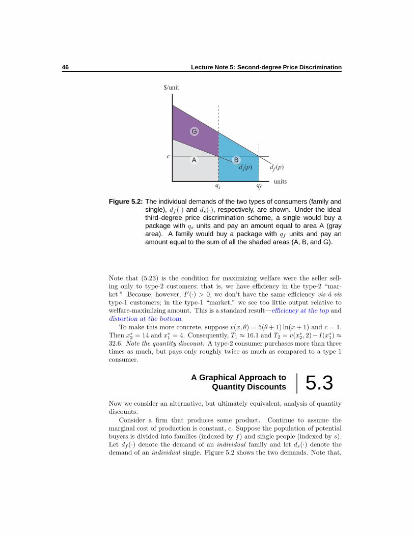
46 Lecture Note 5: Second-degree Price Discrimination
$/unit
units
df (p) ds(p)
c
qs qf
A B
G
Figure 5.2: The individual demands of the two types of consumers (family andsingle), df (·) and ds(·), respectively, are shown. Under the idealthird-degree price discrimination scheme, a single would buy apackage with qs units and pay an amount equal to area A (grayarea). A family would buy a package with qf units and pay anamount equal to the sum of all the shaded areas (A, B, and G).
Note that (5.23) is the condition for maximizing welfare were the seller sell-ing only to type-2 customers; that is, we have efficiency in the type-2 “mar-ket.” Because, however, I ′(·) > 0, we don’t have the same efficiency vis-a-vistype-1 customers; in the type-1 “market,” we see too little output relative towelfare-maximizing amount. This is a standard result—efficiency at the top anddistortion at the bottom.
To make this more concrete, suppose v(x, θ) = 5(θ+ 1) ln(x+ 1) and c = 1.Then x∗2 = 14 and x∗1 = 4. Consequently, T1 ≈ 16.1 and T2 = v(x∗2, 2)− I(x∗1) ≈32.6. Note the quantity discount: A type-2 consumer purchases more than threetimes as much, but pays only roughly twice as much as compared to a type-1consumer.
A Graphical Approach toQuantity Discounts 5.3
Now we consider an alternative, but ultimately equivalent, analysis of quantitydiscounts.
Consider a firm that produces some product. Continue to assume themarginal cost of production is constant, c. Suppose the population of potentialbuyers is divided into families (indexed by f) and single people (indexed by s).Let df (·) denote the demand of an individual family and let ds(·) denote thedemand of an individual single. Figure 5.2 shows the two demands. Note that,
5.3 A Graphical Approach to Quantity Discounts 47
at any price, a family’s demand exceeds a single’s demand.The ideal would be if the firm could engage in third -degree price discrimi-
nation by offering two different two-part tariffs to the two populations. Thatis, if the firm could freely identify singles from families, it would sell to eachmember of each group the quantity that equated that member’s relevant inversedemand to cost (i.e., qs or qf in Figure 5.2 for a single or a family, respectively).It could make the per-unit charge c and the entry fee the respective consumersurpluses. Equivalently—and more practically—the firm could use packaging.The package for singles would have qs units and sell for a single’s total benefit,bs(qs). This is the area labeled A in Figure 5.2. Similarly, the family packagewould have qf units and sell for a family’s total benefit of bf (qf ). This is thesum of the three labeled areas in Figure 5.2.
The ideal is not, however, achievable. The firm cannot freely distinguishsingles from families. It must induce revelation; that is, it must devise a second -degree scheme. Observe that the third-degree scheme won’t work as a second-degree scheme. Although a single would still purchase a package of qs unitsat bs(qs), a family would not purchase a package of qf units at bf (qf ). Why?Well, were the family to purchase the latter package it would, by design, earnno consumer surplus. Suppose, instead, it purchased the package intended forsingles. Its total benefit from doing so is the sum of areas A and G in Figure 5.2.It pays bs(qs), which is just area A, so it would enjoy a surplus equal to areaG. In other words, the family would deviate from the intended package, withqf units, which yields it no surplus, to the unintended package, with qs units,which yields it a positive surplus equal to area G.
Observe that the firm could induce revelation—that is, get the family to buythe intended package—if it cut the price of the qf -unit package. Specifically, ifit reduced the price to the sum of areas A and B, then a family would enjoy asurplus equal to area G whether it purchased the qs-unit package (at price = areaA) or it purchased the intended qf -unit package (at price = area A + area B).Area G is a family’s information rent.
Although that scheme induces revelation, it is not necessarily the profit-maximizing scheme. To see why, consider Figure 5.3. Suppose that the firmreduced the size of the package intended for singles. Specifically, suppose itreduced it to qs units, where qs = qs− h. Given that it has shrunk the package,it would need to reduce the price it charges for it. The benefit that a single wouldderive from qs units is the area beneath its inverse demand curve between 0 andqs units; that is, the area labeled A′. Note that the firm is forgoing revenuesequal to area J by doing this. But the surplus that a family could get bypurchasing a qs-unit package is also smaller; it is now the area labeled G′. Thismeans that the firm could raise the price of the qf -unit package by the arealabeled H. Regardless of which package it purchases, a family can only keepsurplus equal to area G′. In other words, by reducing the quantity sold to the“low type” (a single), the firm reduces the information rent captured by the“high type” (a family).
Is it worthwhile for the firm to trade area J for area H? Observe that the
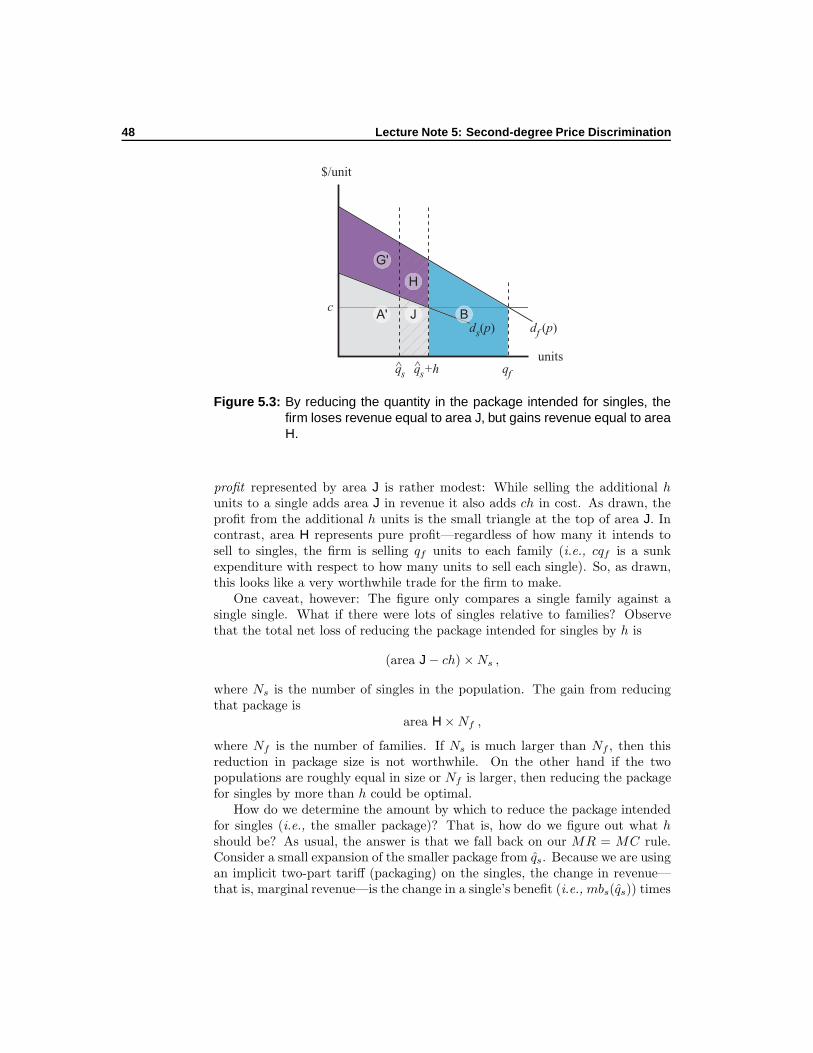
48 Lecture Note 5: Second-degree Price Discrimination
$/unit
units
df (p) ds(p)
c
qf
A' B
G'
J
H
qs+h ^qs ^
Figure 5.3: By reducing the quantity in the package intended for singles, thefirm loses revenue equal to area J, but gains revenue equal to areaH.
profit represented by area J is rather modest: While selling the additional hunits to a single adds area J in revenue it also adds ch in cost. As drawn, theprofit from the additional h units is the small triangle at the top of area J. Incontrast, area H represents pure profit—regardless of how many it intends tosell to singles, the firm is selling qf units to each family (i.e., cqf is a sunkexpenditure with respect to how many units to sell each single). So, as drawn,this looks like a very worthwhile trade for the firm to make.
One caveat, however: The figure only compares a single family against asingle single. What if there were lots of singles relative to families? Observethat the total net loss of reducing the package intended for singles by h is
(area J − ch) ×Ns ,
where Ns is the number of singles in the population. The gain from reducingthat package is
area H ×Nf ,
where Nf is the number of families. If Ns is much larger than Nf , then thisreduction in package size is not worthwhile. On the other hand if the twopopulations are roughly equal in size or Nf is larger, then reducing the packagefor singles by more than h could be optimal.
How do we determine the amount by which to reduce the package intendedfor singles (i.e., the smaller package)? That is, how do we figure out what hshould be? As usual, the answer is that we fall back on our MR = MC rule.Consider a small expansion of the smaller package from qs. Because we are usingan implicit two-part tariff (packaging) on the singles, the change in revenue—that is, marginal revenue—is the change in a single’s benefit (i.e., mbs(qs)) times

5.3 A Graphical Approach to Quantity Discounts 49
the number of singles. That is,
MR(qs) = Nsmbs(qs) .
Recall that the marginal benefit schedule is inverse demand. So if we let ρs(·)denote the inverse individual demand of a single (i.e., ρs(·) = d−1
s (·)), then wecan write
MR(qs) = Nsρs(qs) . (5.24)
What about MC ? Well, if we increase the amount in the smaller package weincur costs from two sources. First, each additional unit raises production costsby c. Second, we increase each family’s information rent (i.e., area H shrinks).Observe that area H is the area between the two demand curves (thus, betweenthe two inverse demand curves) between qs and qs + h. This means that themarginal reduction in area H is
ρf (qs) − ρs(qs) ,
where ρf (·) is the inverse demand of an individual family. Adding them together,and scaling by the appropriate population sizes, we have
MC (qs) = Nsc+Nf(ρf (qs) − ρs(qs)
). (5.25)
Some observations:
1. Observe that if we evaluate expressions (5.24) and (5.25) at the qs shownin Figure 5.2, we have
MR(qs) = Nsρs(qs) and
MC (qs) = Nsc+Nf(ρf(qs) − ρs(qs)
).
Subtract the second equation from the first:
MR(qs) − MC (qs) = Ns(ρs(qs) − c) −Nf(ρf (qs) − ρs(qs)
)
= −Nf(ρf (qs) − ρs(qs)
)
< 0 ,
where the second equality follows because, as seen in Figure 5.2, ρs(qs) = c(i.e., qs is the quantity that equates inverse demand and marginal cost).Hence, provided Nf > 0, we see that the profit-maximizing second-degreepricing scheme sells the low type (e.g., singles) less than the welfare-maximizing quantity (i.e., there is a deadweight loss of area J − ch). Inother words, as we saw previously, there is distortion at the bottom.
2. How do we know we want the family package to have qf units? Well,clearly we wouldn’t want it to have more—the marginal benefit we couldcapture would be less than our marginal cost. If we reduced the packagesize, we would be creating deadweight loss. Furthermore, because we don’t
50 Lecture Note 5: Second-degree Price Discrimination
have to worry about singles’ buying packages intended for families (thatincentive compatibility constraint is slack) we can’t gain by creating sucha deadweight loss (unlike with the smaller package, where the deadweightloss is offset by the reduction in the information rent enjoyed by families).We can summarize this as there being no distortion at the top.
3. Do we know that the profit-maximizing qs is positive? That is, do weknow that a solution to MR = MC exists in this situation? The answeris no. It is possible, especially if there are a lot of families relative tosingles, that it might be profit-maximizing to set qs = 0; that is, sell onlyone package, the qf -unit package, which only families buy. This will bethe case if MR(0) ≤ MC (0). In other words, if
Ns(ρs(0) − c) −Nf(ρf (0) − ρs(0)
)≤ 0 (5.26)
4. On the other hand, it will often be the case that the profit-maximizingqs is positive, in which case it will be determined by equating expressions(5.24) and (5.25).
Extended Example
Consider a cell-phone-service provider. It faces two types of customers, thosewho seldom have someone to talk to (indexed by s) and those who frequentlyhave someone to talked to (indexed by f). Within each population, customersare homogeneous. The marginal cost of providing connection to a cell phone is5 cents a minute (for convenience, all currency units are cents). A member ofthe s-population has demand:
ds(p) =
450 − 10p , if p ≤ 450 , if p > 45
.
A member of the f -population has demand:
df (p) =
650 − 10p , if p ≤ 650 , if p > 65
.
There are 1,000,000 f -type consumers. There are Ns s-type consumers.What is the profit-maximizing second-degree pricing scheme to use? How
many minutes are in each package? What are the prices?It is clear that the f types are the high types (like families in our previous
analysis). There is no distortion at the top, so we know we sell an f type thenumber of minutes that equates demand and marginal cost; that is,
q∗f = df (c) = 600 .
We need to find q∗s . To do this, we need to employ expressions (5.24) and(5.25). They, in turn, require us to know ρs(·) and ρf (·). Considering the

5.3 A Graphical Approach to Quantity Discounts 51
regions of positive demand, we have:
qs = 450 − 10ρs(qs) and
qf = 650 − 10ρf(qf ) ;
hence,
ρs(qs) = 45 − qs10
and
ρf (qf ) = 65 − qf10.
Using expression (5.24), marginal revenue from qs is, therefore,
MR(qs) = Nsρs(qs) = Ns ×(45 − qs
10
).
Marginal cost of qs (including forgone surplus extraction from the f type) is
MC(qs) = Nsc+Nf(ρf (qs) − ρs(qs)
)
= 5Ns + 1, 000, 000(65 − qf
10− 45 +
qf10
)
= 5Ns + 20, 000, 000 .
Do we want to shut out the s-types altogether? Employing expression (5.26),the answer is yes if
40Ns − 20, 000, 000 < 0 ;
that is, if
Ns < 500, 000 .
So, if Ns < 500, 000, then q∗s = 0 and the price for 600 minutes (i.e., q∗f ) isbf(600), which is
bf (600) = Area under ρf (·) from 0 to 600
=
∫ 600
0
ρf (z)dz
=
∫ 600
0
(65 − z
10
)dz
= 21, 000
cents or $210.Suppose that Ns ≥ 500, 000. Then, equating MR and MC, we have
Ns ×(45 − qs
10
)= 5Ns + 20, 000, 000 ;
52 Lecture Note 5: Second-degree Price Discrimination
hence,
q∗s = 400 − 200, 000, 000
Ns.
The low type retains no surplus, so the price for q∗s minutes is bs(q∗s ), which
equals the area under ρs(·) from 0 to q∗s . This can be shown (see derivation ofbf (600) above) to be
bs(q∗s ) = Area under ρs(·) from 0 to q∗s
=
∫ q∗s
0
(45 − q
10
)dq
= 45q∗s −q∗s
2
20.
The price charged the f types for their 600 minutes is bf (600) less their infor-mation rent, which is the equivalent of area G′ in Figure 5.3.
Area G′ =
∫ q∗s
0
(65 − q
45− 45 +
q
45
)dq = 20q∗s .
So the price charged for 600 minutes is 21, 000− 20q∗s cents ($210 − q∗s/5).To conclude: If Ns < 500, 000, then the firm sells only a package with 600
minutes for $210. In this case, only f types buy. If Ns ≥ 500, 000, then thefirm sells a package with 600 minutes, purchased by the f types, for 210− q∗s/5dollars; and it also sells a package with q∗s minutes for a price of bs(q
∗s) dollars.
For example, if Ns = 5, 000, 000, then the two plans are (i) 600 minutes for$138; and (ii) 360 minutes for $97.20.
A General Analysis 5.4Although presented in different ways, the various forms of second-degree pricediscrimination are all examples of mechanism design. As such, they can bemodeled in a general way.
Assume there is a measure of consumers, which we can take to be one withoutloss of generality. Each consumer has a type, θ, where θ ∈ [θ, θ]. Types are dis-tributed according to the distribution function F : [θ, θ] → [0, 1]. Assume F (·)is differentiable and denote its derivative—the associated density function—byf(·). Assume f(θ) > 0 for all θ ∈ [θ, θ] (i.e., f(·) has full support).2
A consumer’s utility is u(q, θ) + y, where y is the numeraire good and q ∈R+ is either the quantity of the other good—the good being sold by the firmengaging in second-degree price discrimination—or the quality of that good. Inthe latter case, assume the consumer buys, at most, a single unit of the good.
2A similar analysis could be carried out with a discrete type space, but not as straightfor-wardly.

5.4 A General Analysis 53
Assume that the marginal utility from more q is increasing with type (one canthink of this as the definition of type); specifically,
∂
∂θ
∂u(q, θ)
∂q=∂2u(q, θ)
∂θ∂q> 0 (5.27)
for all q and θ.3 Assume u(0, θ) is the same regardless of type; that is, u(0, θ) =u(0, θ′) for any θ and θ′. When q is quantity, this assumption is relativelyinnocuous. It could be more of an issue when q is quality—conceivably differenttypes could derive different utility from the lowest-quality product. A wayaround that is to imagine that a product of quality 0 is the same as not buyingthe product at all. It is without further loss of generality to assume u(0, θ) = 0for all θ.
The seller incurs a cost of c(q) to produce either a package with q units init or a product with quality q. Assume c′(q) > 0 for all q. For each type θ, wecan consider the seller as determining a package or product, q(θ), that it willsell for t(θ) and that only θ-type consumers will buy. Because q(θ) and t(θ)could equal zero, there is no loss of generality in assuming all consumers “buy”in equilibrium (i.e., we can consider those who don’t buy as “buying” q = 0 atprice of 0).
The firm’s problem then is to choose 〈q(·), t(·)〉 to maximize profit
∫ θ
θ
(t(θ) − c
(q(θ)
))f(θ)dθ (5.28)
subject to the constraint that consumers prefer to buy rather than not buy,
u(q(θ), θ
)− t(θ) ≥ 0 for all θ , (ir)
and subject to the constraint that each type of consumer buy the package orproduct intended for him,
u(q(θ), θ
)− t(θ) ≥ u
(q(θ), θ
)− t(θ) for all θ, θ . (ic)
As written, this is a difficult optimization program to solve because of thenature of the incentive-compatibility (revelation) constraints (ic). To makeprogress, we need to do some analysis. Consider two types θ1 and θ2 withθ1 < θ2. The ic constraints imply:
u(q(θ1), θ1
)− t(θ1) ≥ u
(q(θ2), θ1
)− t(θ2) and
u(q(θ2), θ2
)− t(θ2) ≥ u
(q(θ1), θ2
)− t(θ1) .
As is often the case in mechanism-design problems, it is easier to work withutilities than payments. To this end, define
v(θ) = u(q(θ), θ
)− t(θ) .
3Expression (5.27) is the Spence-Mirrlees or single-crossing condition for this problem.

54 Lecture Note 5: Second-degree Price Discrimination
v(θ) is the θ-type consumer’s equilibrium utility. Observe the utility a θ-type
consumer gets from buying the product or package intended for the θ-typeconsumer can be written as
v(θ) − u(q(θ), θ
)+ u(q(θ), θ
).
We can, therefore, write the pair of inequalities above as
v(θ1) ≥ v(θ2) − u(q(θ2), θ2
)+ u(q(θ2), θ1
)and
v(θ2) ≥ v(θ1) − u(q(θ1), θ1
)+ u(q(θ1), θ2
).
These inequalities can be combined as
∫ θ2
θ1
∂u(q(θ1), z
)
∂θdz ≤ v(θ2) − v(θ1) ≤
∫ θ2
θ1
∂u(q(θ2), z
)
∂θdz . (5.29)
Expression (5.29) has two consequences. First, ignoring the middle term, itimplies ∫ θ2
θ1
∫ q(θ2)
q(θ1)
∂2u(q, z)
∂q∂θdq dz ≥ 0 .
From (5.27), we know the cross-partial derivative is everywhere positive. Givenθ1 < θ2, this means the double integral can be non-negative only if q(θ1) ≤ q(θ2).Because θ1 and θ2 are arbitrary, we can conclude that the quantity/qualityfunction, q(·), is non-decreasing in type. That is, if the second-degree pricediscrimination scheme is incentive compatible, then lower types cannot get morequantity/quality than higher types.
The second consequence of (5.29) is derived as follows. By fixing one endpoint (i.e., θ1 or θ2) and letting the other converge towards it, we see that v(·) isabsolutely continuous with respect to the Lebesgue measure and is, thus, almosteverywhere differentiable. This derivative is
dv(θ)
dθ=∂u(q(θ), θ
)
∂θ
almost everywhere.4 Integration reveals that
v(θ) = v(θ) +
∫ θ
θ
∂u(q(z), z
)
∂θdz . (5.30)
The analysis to this point has established (i) a necessary condition for asecond-degree price discrimination scheme to be incentive compatible is thatthe quality/quantity function q(·) be non-decreasing; and (ii) another necessary
4Note the important distinction between∂u
`
q(θ),θ´
∂θand
du`
q(θ),θ´
dθ. The former is the
partial derivative of u with respect to to second argument evaluated at`
q(θ), θ´
, while thelatter is the total derivative of u.

5.4 A General Analysis 55
condition for incentive compatibility is that (5.30) hold. The latter is equivalent,recalling the definition of v(·), to saying the payment function must satisfy
t(θ) = tL + u(q(θ), θ
)−∫ θ
θ
∂u(q(z), z
)
∂θdz , (5.31)
where tL = −v(θ) is a constant.It turns out that (i) and (ii) are also sufficient conditions, which means,
given our initial assumptions, that we can restrict attention without loss topricing schemes in which q(·) is non-decreasing and t(·) is given by (5.31).
Proposition 8 Under the assumptions of this section, a second-degree pricediscrimination scheme 〈q(·), t(·)〉 is incentive compatible if and only if t(·) is asstated in expression (5.31) and q(·) is non-decreasing.
Proof: Necessity was established in the text. Consider a second-degree price-discrimination scheme that satisfies (5.31) (equivalently, (5.30)) and has q(·)non-decreasing. We need to establish that such a scheme induces a type-θconsumer to prefer to purchase q(θ) at t(θ) than to pursue another option. Hisutility if he purchases q(θ′) at t(θ′), θ′ > θ, is
u(q(θ′), θ
)− t(θ′)
= −tL + u(q(θ′), θ
)− u(q(θ′), θ′
)+
∫ θ
θ
∂u(q(z), z
)
∂θdz +
∫ θ′
θ
∂u(q(z), z
)
∂θdz
= u(q(θ), θ
)− t(θ) −
∫ θ′
θ
(∂u(q(θ′), z
)
∂θ− ∂u
(q(z), z
)
∂θ
)dz
= v(θ) −∫ θ′
θ
∫ q(θ′)
q(z)
∂2u(q, z)
∂q∂θdqdz ≤ v(θ) ,
where the third line follows from the second by adding and subtracting u(q(θ), θ
),
the definition of t(θ), and recognizing that
u(q(θ′), θ
)− u(q(θ′), θ′
)= −
∫ θ′
θ
∂u(q(θ′), z
)
∂θdz ;
the final inequality follows because q(·) is non-decreasing, so the direction ofintegration in the inner integral of the fourth line is the positive direction and,by (5.27), the function being integrated is positive. Because we established
u(q(θ′), θ
)− t(θ′) ≤ v(θ) ,
we have shown that the mechanism is incentive compatible insofar as a typeθ would not choose a package/product intended for a higher type. Exercise:finish the proof of sufficiency for the case θ′ < θ.

56 Lecture Note 5: Second-degree Price Discrimination
In light of Proposition 8, the firm’s problem is to choose 〈q(·), t(·)〉 to max-imize (5.28) subject to (ir) and q(·) non-decreasing with t(·) being given by(5.31). It is again easier to work with v(·) than t(·), where v(·) is given by(5.30). This makes the firm’s problem:
max〈q(·),v(·)〉
∫ θ
θ
(u(q(θ), θ
)−∫ θ
θ
∂u(q(z), z
)
∂θdz − v(θ)
︸ ︷︷ ︸−v(θ)︸ ︷︷ ︸
t(θ)
−c(q(θ)
))f(θ)dθ (5.32)
subject to
v(θ) ≥ 0 ∀θ (5.33)
and
q(·) non-decreasing (5.34)
Observe that
u(q(θ), θ
)− c(q(θ)
)≡ w
(q(θ), θ
)
is the welfare generated by trade with a type-θ consumer. Comparing thatexpression with (5.32), we see that the firm’s objective is quite different thanwelfare maximization. Consequently, as will be verified below, we should notexpect the firm’s choice of a second-degree price-discrimination scheme to max-imize welfare.
Using the above definition of w(·, ·), the firm’s objective function can berewritten as
∫ θ
θ
(w(q(θ), θ
)−∫ θ
θ
∂u(q(z), z
)
∂θdz
)f(θ)dθ − v(θ)
=
∫ θ
θ
(w(q(θ), θ
)− 1 − F (θ)
f(θ)
∂u(q(θ), θ
)
∂θ
)f(θ)dθ − v(θ) , (5.35)
where the second line follows from integration by parts. The expression
1 − F (θ)
f(θ)(5.36)
is the multiplicative inverse of the hazard rate (this inverse is sometimes calledthe Mills ratio). Many distributions have the property that their hazard rateis non-decreasing (among these distributions are the uniform, the normal, andthe exponential). If the hazard rate is non-decreasing, then expression (5.36) isnon-increasing in θ. We give a name to this property:
5.4 A General Analysis 57
Assumption 1 (MHRP) Assume the hazard rate associated with the distri-bution of types exhibits the monotone hazard rate property, which is to say it isa non-decreasing function.
We will assume, henceforth, that F (·) satisfies the mhrp; that is, that expression(5.36) is non-increasing in θ.
Lemma 6 The function u(q, ·) is increasing for q > 0.
Proof: From (5.27)∂u(q, θ′)
∂q>∂u(q, θ)
∂q
for all q whenever θ′ > θ. Hence,∫ q
0
(∂u(z, θ′)
∂q− ∂u(z, θ)
∂q
)dz > 0
for all q. Hence,
0 <(u(q, θ′) − u(q, θ)
)−(u(0, θ′) − u(0, θ)
)= u(q, θ′) − u(q, θ) ,
where the equality follows because, recall, we assumed u(0, θ) = 0 for all θ.In light of Lemma 6, we have ∂u(q, θ)/∂θ > 0 for all q > 0. Consequently, from(5.30), we have v(θ) ≥ v(θ) for all θ > θ. This means that if the ir constraint issatisfied for type θ it is satisfied for all types. Because, from (5.35), the firm’sprofits are decreasing in v(θ), the firm wants to make v(θ) as small as possible.Given the ir constraint, this means that the firm sets v(θ) = 0.
Corollary 2 Optimally, the firm sets v(θ) = 0. The ir constraint is met forall types.
Observe this portion of the analysis reveals that the lowest type keeps no con-sumer surplus; a result that is consistent with our analysis in earlier sections.
Having set v(θ) = 0, the firm’s problem boils down to maximizing (5.35)subject to the constraint that q(·) be non-decreasing. In general, this is anoptimal-control problem. Fortunately, in many contexts, the problem can besolved simply by maximizing (5.35) pointwise; that is, solve
maxqw(q, θ)− 1 − F (θ)
f(θ)
∂u(q, θ)
∂θ. (5.37)
Provided the solutions yield a non-decreasing q(·), we’re done. Observe, exceptwhen θ = θ (and, thus, 1 − F (θ) = 0), the solution to (5.37) will not maximizewelfare. In particular, from the Spence-Mirrlees condition—that is, expression(5.27)—we know that derivative of (5.37) lies below the derivative of w(·, θ) forall θ < θ; hence, the solution to (5.37) will be less than the welfare-maximizingsolution. To conclude:
Proposition 9 The quantity/quality provided the highest type is the welfare-maximizing amount (no distortion at the top). For all other types, however, thequantity/quality provided is less than the welfare-maximizing amount (downwarddistortion below the top).

58 Lecture Note 5: Second-degree Price Discrimination
A quantity-discount example
Suppose that c(q) = cq, c > 0, and u(q, θ) = θ log(q + 1). Observe the welfare-maximizing package for a type-θ consumer is (θ − c)/c. Suppose that types aredistributed uniformly from c + γ to c + γ + 1, γ ≥ 0. Observe f(θ) = 1 and1 − F (θ) = c+ γ + 1 − θ. Expression (5.37) is, thus,
θ log(q+1)−cq−(c+γ+1−θ) log(q+1) = 2θ log(q+1)−cq−(c+γ+1) log(q+1)
The maximum is
q(θ) =
0 , if θ ≤ c+ γ+1
2
2θ−2c−γ−1c
, if θ > c+ γ+12
.
Because q(·) is non-decreasing, this is indeed the optimum for the firm. From(5.31) we have
t(θ) = θ log(q(θ) + 1
)−∫ θ
c+γ
log(q(z) + 1
)dz
Some observations, if γ < 1, then some types are shut out of the market;that is, the firm does not offer a package that the lowest types wish to purchase.
If we assume c = γ = 1, then all types except θ = 2 are served; the size oftheir package is 2θ − 4. A type-θ consumer pays
θ − 2 +3
2log(2θ − 3) .
Dividing the price of each package by its quantity (i.e., calculating t(θ)/q(θ))we get
1
2+
3 log(2θ − 3)
4θ − 8. (5.38)
It is readily verified that (5.38) is a decreasing function of θ; that is, there arequantity discounts.
A quality-distortion example
Suppose that the cost of a product with quality q is q2/2. Suppose types aredistributed uniformly on [1, 2]. Finally, suppose that u(q, θ) = θq. It is readilychecked that the welfare-maximizing quality to offer a type-θ consumer is q = θ.The firm’s problem, expression (5.37), is
maxqθq − q2
2− (2 − θ)q ≡ max
q2(θ − 1)q − q2
2.
The solution is q(θ) = 2(θ−1), which is increasing in θ and, thus, a valid solution.Observe that type 1 is just shut out (i.e., q(1) = 0). Note there is downwarddistortion, except at the top: 2(θ−1) < θ for all θ < 2 and 2(θ−1) = θ if θ = 2.From (5.31),
t(θ) = θ(2(θ − 1)
)−∫ θ
1
2(z − 1)dz = θ2 − 1 .

Mechanism Design
59

Purpose
Our purpose is to consider the problem of hidden information; that is, a gamebetween two economic actors, one of whom possesses mutually relevant informa-tion that the other does not. This is a common situation: The classic example—covered in the previous part of these lecture notes—being the “game” betweena monopolist, who doesn’t know the consumer’s willingness to pay, and theconsumer, who obviously does. Within the realm of contract theory, relevantsituations include a seller who is better informed than a buyer about the costof producing a specific good; an employee who alone knows the difficulty ofcompleting a task for his employer; a divisional manager who can conceal infor-mation about his division’s investment opportunities from headquarters; and aleader with better information than her followers about the value of pursuinga given course of action. In each of these situations, having private informa-tion gives the player possessing it a potential strategic advantage in his dealingswith the other player. For example, consider a seller who has better informationabout his costs than his buyer. By behaving as if he had high costs, the sellercan seek to induce the buyer to pay him more than she would if she knew hehad low costs. That is, he has an incentive to use his superior knowledge tocapture an “information rent.” Of course, the buyer is aware of this possibility;so, if she has the right to propose the contract between them, she will proposea contract that works to reduce this information rent. Indeed, how the con-tract proposer—the principal—designs contracts to mitigate the informationaldisadvantage she faces will be a major focus of this part of the lecture notes.
Bibliographic Note
This part of the lecture notes draws heavily from a set of notes that I co-authoredwith Bernard Caillaud.
Not surprisingly, given the many applications of the screening model, thiscoverage cannot hope to be fully original. The books by Laffont and Tirole(1993) and Salanie (1997) include similar chapters. Surveys have also appearedin journals (e.g., Caillaud et al., 1988). Indeed, while there are idiosyncraticaspects to the approach pursued here, the treatment is quite standard.
61

62 Purpose

The Basics ofContractual
Screening 6Let us begin by broadly describing the situation in which we are interested. Weshall fill in the blanks as we proceed through this reading.
• Two players are involved in a strategic relationship; that is, each player’swell being depends on the play of the other player.
• One player is better informed (or will become better informed) than theother; that is, he has private information about some state of naturerelevant to the relationship. As is typical in information economics, wewill refer to the player with the private information as the informed playerand the player without the private information as the uninformed player.
• Critical to the analysis of these situations is the bargaining game thatdetermines the contract. Call the contract proposer the principal andcall the player who receives the proposal the agent. Moreover, assumecontracts are proposed on a take-it-or-leave-it (tioli) basis: The agent’sonly choices are to accept or reject the contract proposed by the principal.Rejection ends the relationship between the players. A key assumptionis that the principal is the uninformed player. Models like this, in whichthe uninformed player proposes the contract, are referred to as screeningmodels. In contrast, were the informed player the contract proposer, wewould have a type of signaling model.
• A contract can be seen as setting the rules of a secondary game to beplayed by the principal and the agent.
The asymmetry of information that exists in this game results because priorexperience or expertise, location, or other factors give the agent free access toinformation about the state of nature; while the absence of expertise, differentexperience or location, or other factors exclude the principal from this infor-mation (make it prohibitively expensive for her to acquire it). For example,past jobs may tell a seller how efficient he is—and thus what his costs will be—while ignorance of these past jobs means the buyer has a less precise estimateof what his costs will be. The reason for this asymmetry of information is takento be exogenous. In particular, the informed player is simply assumed to beendowed with his information. Here, note, only one player is better informed;that is, we are ruling out situations where each player has his or her own private
63
64 Lecture Note 6: The Basics of Contractual Screening
information.1
Given this information structure, the two parties interact according to somespecified rules that constitute the extensive form of a game. In this two-persongame, the players must contract with each other to achieve some desired out-come. In particular, there is no ability to rely on some exogenously fixed andanonymous market mechanism. My focus will be on instances of the game wherethe informed player can potentially benefit from his informational advantage(e.g., perhaps inducing a buyer to pay more for a good than necessary becauseshe fears the seller is high cost). But, because the informed player doesn’t havethe first move—the uninformed player gets to propose the contract—this infor-mational advantage is not absolute: Through her design of the contract, theuninformed player will seek to offset the informed player’s inherent advantage.
1Put formally, the uninformed player’s information partition is coarser than the informedplayer’s information partition.
The Two-typeScreening Model 7
I will begin to formalize these ideas in as simple a model as possible, namelythe two-type model. In the two-type model, the state of nature can take one oftwo possible values. As is common in this literature, I will refer to the realizedstate of nature as the agent’s type. As there are only two possible states, theagent can have one of just two types.
Before proceeding, however, it needs to be emphasized that such simplicityin modeling is not without cost. The two-type model is “treacherous,” in sofar as it may suggest conclusions that seem general, but which are not. Forexample, the conclusion that we will shortly reach with this model that theoptimal contract implies distinct outcomes for distinct states of nature—a resultcalled separation—is not as general as it may seem. Moreover, the assumptionof two types conceals, in essence, a variety of assumptions that must be madeclear. It similarly conceals the richness of the screening problem in complex,more realistic, relationships. Few economic prescriptions and predictions shouldbe reached from considering just the two-type model. Keeping this admonitionin mind, we now turn to a simple analysis of private procurement in a two-typemodel.
A simple two-type screeningsituation 7.1
A large retailer (the principal) wishes to purchase units of some good for resale.Assume its size gives it all the bargaining power in its negotiations with the onefirm capable of supplying this product (the agent). Let x ∈ R+ denote the unitsof this good and let r (x) denote the retailer’s revenues from x units.1 Assumethat r (·) is strictly concave and differentiable everywhere. Assume, too, thatr′ (0) > 0. (Because r (·) is a revenue function, r (0) = 0.)
The retailer is uncertain about the efficiency of the supplier. In particular,the retailer knows an inefficient supplier has production costs of CI (x), butan efficient supplier has production costs of CE (x). Let the retailer’s priorbelief be that the supplier is inefficient with probability f , where—reflecting itsuninformed status—0 < f < 1. The supplier, in contrast, knows its type; thatis, whether it is efficient or not.
1For convenience, assume that the retailer incurs no costs other than those associated withacquiring the x units from the supplier. Alternatively, one could simply imagine that theseother costs have been subtracted from revenues, so that r (x) is profit gross of the cost ofpurchasing the x units.
65

66 Lecture Note 7: The Two-type Screening Model
Assume Ct (·) is increasing, everywhere differentiable, and convex for bothtypes, t. (Because Ct (·) is a cost function, we know Ct (0) = 0.) Consistent withthe ideas that the two types correspond to different levels of efficiency, we assumeC′I (x) > C′
E (x) for all x > 0—the inefficient type’s marginal-cost schedule liesabove the efficient type’s. Observe, necessarily then, that CI (x) > CE (x) forall x > 0.
The retailer and the supplier have to agree on the quantity, x, of the goodto trade and on a payment, s, for this total quantity. Please note that s isnot the per-unit price, but the payment for all x units. Profits for retailer andsupplier are, then, r(x) − s and s − Ct(x) respectively. The retailer makes atake-it-or-leave-it offer, which the supplier must either accept or refuse. If thesupplier refuses the offer, there is no trade and each firm’s payoff from this“transaction” is zero. This outcome, no agreement, is equivalent to agreeing totrade 0 units for a 0 payment. Hence, it is without loss of generality to assumethat the parties must reach some agreement in equilibrium.
We begin our analysis with the benchmark case of symmetric or full infor-mation. That is, for the moment, assume the retailer knew the supplier’s type(i.e., f = 0 or f = 1). We may immediately characterize the Pareto optimalallocation: xFt units are traded, where
xFt = arg maxx≥0
r(x) − Ct(x) .
Because the problem is otherwise uninteresting if trade is never desirable, as-sume that r′(0) > C′
E(0) so that, with an efficient supplier at least, some trade isdesirable. Pareto optimality, also referred to as ex post efficiency , then reducesto
r′(xFE) = C′E(xFE) and
[r′(xFI)− C′
I
(xFI)]xFI = 0
(where we take the larger non-negative root of the second equation). As itis optimal to produce a greater amount when marginal costs are lower, ourassumptions about C′
t (·) imply 0 ≤ xFI < xFE . In making its contract offer, theretailer sets x = xFt and it offers a payment, sFt , no larger than necessary toinduce the supplier to accept; that is, sFt satisfies
sFt − Ct(xFt ) = 0.
Contracts under IncompleteInformation 7.2
This symmetric-information (benchmark) solution collapses when the retailer isuninformed about the state of nature. To see why, suppose that the retaileroffered the supplier its choice of
⟨xFE , s
FE
⟩or⟨xFI , s
FI
⟩with the expectation that
the supplier would choose the one appropriate to its type (i.e., the first contractif it were efficient and the second if it were not). Observe that the retailer isrelying on the supplier to honestly disclose its type. Suppose, moreover, thatthe true state of nature is E. By truthfully revealing that the state of nature
7.2 Contracts under Incomplete Information 67
is E, the supplier would just be compensated for its cost of supplying xFE units;that is, it would earn a profit of sFE − CE(xFE) = 0. On the other hand, if thesupplier pretends to have high costs—claims the state of nature is I—it receivescompensation sFI , while incurring cost CE(xFI ) for supplying xFI units. Thisyields the supplier a profit of
sFI − CE(xFI)
=
CI(xFI ) − CE(xFI ) > 0
(recall sFI = CI(xFI)). Clearly, then, the efficient-type supplier cannot be relied
on to disclose its type honestly.This difference or profit, CI(x
FI )−CE(xFI ), which motivates the supplier to
lie, is called an information rent. This is a loss to the retailer but a gain tothe supplier. There is, however, an additional loss suffered by the retailer thatis not recaptured by the supplier: Lying means inefficiently little is produced;that is, a real deadweight loss of
[r(xFE)− CE
(xFE)]
−[r(xFI)− CE
(xFI)]
is suffered.Given this analysis, it would be surprising if the retailer would be so naıve as
to rely on the supplier to freely reveal its type. In particular, we would expectthe retailer to seek a means of improving on this ex post inefficient outcome bydevising a more sophisticated contract. What kind of contracts can be offered?Because the retailer does not know the supplier’s level of efficiency, it may wantto delegate the choice of quantity to the supplier under a payment schedule thatimplicitly rewards the supplier for not pretending its costs are high when theyare truly low. This payment schedule, S(·), specifies what payment, s = S(x),is to be paid the supplier as a function of the units, x, it chooses to supply.Wilson (1993) provides evidence that such payment schedules are common inreal-world contracting.
If the supplier accepts such a contract, the supplier’s choice of quantity, xt,is given by
xt ∈ arg maxx≥0
S(x) − Ct(x) . (7.1)
Assume for the moment that this program has a unique solution. Let ut denotethe value of this maximization program and let st = S(xt) be the supplier’spayment under the terms of the contract. By definition,
ut = st − Ct(xt).
Observe that this means we can write the equilibrium payment, st, as
st = ut + Ct (xt) .
DefineR (·) = CI (·) − CE (·)

68 Lecture Note 7: The Two-type Screening Model
as the information-rent function. Our earlier assumptions imply that R (·) ispositive for x > 0, zero for x = 0, and strictly increasing.
Revealed preference in the choice of x necessarily implies the following aboutxI and xE :
uE = sE − CE(xE) ≥ sI − CE(xI) = uI +R(xI) (7.2)
uI = sI − CI(xI) ≥ sE − CI(xE) = uE −R(xE). (7.3)
These inequalities are referred by many names in the literature: incentive-compatibility constraints, self-selection constraints, revelation constraints, andtruth-telling constraints. Regardless of name, they simply capture the require-ment that (xI , sI) and (xE , sE) be the preferred choices for the supplier in statesI and E, respectively.
What can we conclude from expressions (7.2) and (7.3)? First, rewritingthem as
R(xI) ≤ uE − uI ≤ R(xE), (7.4)
we see thatxI ≤ xE , (7.5)
because R(·) is strictly increasing. Observe, too, that expression (7.2) impliesuE > uI (except if xI = 0, in which case we only know uE ≥ uI). Finally,expressions (7.2) and (7.5) implies sE > sI (unless xE = xI , in which case (7.2)and (7.3) imply sE = sI).
Of course the contract—payment schedule S (·)—must be acceptable to thesupplier, which means
uI ≥ 0; and (7.6)
uE ≥ 0 . (7.7)
If these did not both hold, then the contract would be rejected by one or theother or both types of supplier. The constraints (7.6) and (7.7) are referred toas the agent’s participation or individual-rationality constraints. They simplystate that, without any bargaining power, the supplier accepts a contract if andonly if accepting does not entail suffering a loss.
The retailer’s problem is to determine a price schedule S(·) that maximizesits expected profit (“expected” because, recall, it knows only the probabilitythat a give type will be realized). Specifically, the retailer seeks to maximize
f × [r(xI ) − sI ] + (1 − f) × [r(xE) − sE ] ; or, equivalently,
f × [r(xI ) − CI (xI) − uI ] + (1 − f) × [r(xE) − CE (xE) − uE ] ,
where (xt, ut) are determined by the supplier’s optimization program (7.1) inresponse to S(·).
Observe that only two points on the whole price schedule enter the retailer’sobjective function: (xI , sI) and (xE , sE); or, equivalently, (xI , uI) and (xE , uE).The maximization of the principal’s objectives can be performed with respect to

7.2 Contracts under Incomplete Information 69
just these two points provided that we can recover a general payment scheduleafterwards such that the supplier would accept this schedule and choose theappropriate point for its type given this schedule. For this to be possible, weknow that the self-selection constraints, (7.2) and (7.3), plus the participationconstraints, (7.6) and (7.7), must hold.
In fact, the self-selection constraints and the participation constraints on(xI , sI) and (xE , sE) are necessary and sufficient for there to exist a paymentschedule such that the solution to (7.1) for type t is (xt, st). To prove thisassertion, let (xI , sI) and (xE , sE) satisfy those constraints and construct therest of the payment schedule as follows:
S(x) = 0 if 0 ≤ x < xI= sI if xI ≤ x < xE= sE if xE ≤ x,
when 0 < xI < xE .2 Given that Ct(·) is increasing in x, no supplier wouldever choose an x other than 0, xI , or xE (the supplier’s marginal revenue iszero except at these three points). The participation constraints ensure that(xt, st) is (weakly) preferable to (0, 0) and the self-selection constraints ensurethat a type-t supplier prefers (xt, st) to (xt′ , st′), t 6= t′. That is, we’ve shownthat faced with this schedule, the type-I supplier’s solution to (7.1) is (xI , sI)—as required—and that the type-E supplier’s solution to (7.1) is (xE , sE)—asrequired.
The retailer’s problem can thus be stated as
maxxI ,xE ,uI ,uE
f×[r(xI ) − CI (xI) − uI ]+(1−f)×[r(xE) − CE (xE) − uE ] (7.8)
subject to (7.2), (7.3), (7.6), and (7.7). Solving this problem using the standardLagrangean method is straightforward, albeit tedious. Because, however, sucha mechanical method provides little intuition, we pursue a different, thoughequivalent, line of reasoning.
• One can check that ignoring the self-selection constraints (treating themas not binding) leads us back to the symmetric-information arrangement;and we know that at least one self-selection constraint is then violated.We can, thus, conclude that in our solution to (7.8) at least one of theself-selection constraints is binding.
• The self-selection constraint in state E implies that: uE ≥ R(xI) + uI ≥uI . Therefore, if the supplier accepts the contract in state I, it will alsoaccept it in state E. We can, thus, conclude that constraint (7.7) is slackand can be ignored.
• It is, however, the case that (7.6) must be binding at the optimum: Sup-pose not, then we could lower both utility terms uL and uH by some
2If xI = 0, then sI = 0. If xI = xE , then sI = sE .
70 Lecture Note 7: The Two-type Screening Model
ε > 0 without violating the participation constraints. Moreover, given thetwo utilities have been changed by the same amount, this can’t affect theself-selection constraints. But, from (7.8), lowering the utilities raises theprincipal’s profits—which means our “optimum” wasn’t optimal.
• Using the fact that (7.6) is binding, expression (7.4)—the pair of self-selection constraints—reduces to
R(xI) ≤ uE ≤ R(xE).
Given a pair of quality levels (xI , xE), the retailer wants to keep thesupplier’s rent as low as possible and will, therefore, choose to pay himthe smallest possible information rent; that is, we can conclude that uE =R(xI). The self-selection constraint (7.2) is, thus, slack, provided thenecessary monotonicity condition (7.5) holds.
Plugging our findings, uI = 0 and uE = R(xI), into the retailer’s objectivesyields the following reduced program:
max(xI ,xE)| xI≤xE
f × [r(xI ) − CI(xI)] + (1 − f) × [r(xE) − CE(xE) −R(xI)] .
The solution is
xE = xFE = argmaxx≥0
r(x) − CE(x) (7.9)
xI = x∗I(f) ≡ arg maxx≥0
r(x) − CI(x) −
1 − f
fR(x)
. (7.10)
The only step left is to verify that the monotonicity condition (7.5) is satisfiedfor these values. If we consider the last two terms in the maximand of (7.10)to be cost, we see that the effective marginal cost of output from the inefficienttype is
C′I (x) +
1 − f
fR′ (x) > C′
I (x) > C′E (x)
for x > 0.3 The greater the marginal-cost schedule given a fixed marginal-revenue schedule, the less is traded; that is, it must be that x∗I(f) < xFE—themonotonicity condition (7.5) is satisfied.
It is worth summarizing the nature and properties of the optimal price sched-ule for the retailer to propose:
Proposition 10 The optimal (non-linear) payment schedule for the principalinduces two possible outcomes depending upon the state of nature such that:
• the supplier trades the ex post efficient quantity, xFE, when it is an efficientproducer, but trades less than the efficient quantity when it is an inefficientproducer (i.e., x∗I(f) < xFI );
3Because xFE
> 0, this is the relevant domain of output to consider.

7.2 Contracts under Incomplete Information 71
• an inefficient supplier makes no profit (uI = 0), but an efficient supplierearns an information rent of R [x∗I(f)];
• the revelation constraint is binding in state E, slack in state I;
• the participation constraint is binding in state I, slack in state E;
• x∗I(f) and R [x∗I(f)] are non-decreasing in the probability of drawing aninefficient producer (i.e., are non-decreasing in f);
• and, finally, limf↓0 x∗I(f) = 0, limf↑1 x∗I(f) = xFI , limf↓0R [x∗I(f)] = 0,and limf↑1R [x∗I(f)] = R(xFI ).
To see that the last two points hold, note first that the effective marginal costof production from an inefficient supplier,
C′I (x) +
1 − f
fR′ (x) ,
is falling in f . By the usual comparative statics, this means that x∗I (f) is non-decreasing. Since R (·) is an increasing function, R [x∗I(f)] must be similarlynon-decreasing. As f ↓ 0, this effective marginal cost tends to +∞ for x > 0,which means the optimal level of trade falls to zero. As f ↑ 1, this effectivemarginal cost tends to the symmetric-information marginal cost, hence x∗I (f)tends to the symmetric-information level, xFI .
Intuition for these results can be gained from Figure 7.1. This figure showsone indifference curve for an inefficient (type-I) supplier and three indifferencecurves for an efficient (type-E) supplier in output-payment space. The type-Iindifference curve is that type’s zero-profit curve (hence, by necessity, it passesthrough the origin). Correspondingly, the lowest and darkest of the type-Eindifference curves is that type’s zero-profit curve. The faint dash-dot linesare iso-profit curves for the retailer (to minimize clutter in the figure, they’resketched as straight lines, but this is not critical for what follows). Observethat an iso-profit curve is tangent to type-I’s zero-profit indifference curve atpoint A. Likewise, we have similar tangency for type-E at point B. Hence—under symmetric information—points A and B would be the contracts offered.Under asymmetric information, however, contract B is not incentive compatiblefor type-E: Were it to lie and claim to be type-I (i.e., move to point A),then it would be on a higher (more profitable) indifference curve (the highestof its three curves). Under asymmetric information, an incentive compatiblepair of contracts that induce the symmetric-information levels of trade are Aand C. The problem with this solution, however, is that type-E earns a largeinformation rent, equal to the distance between B and C. The retailer can reducethis rent by distorting downward the quantity asked from a type-I supplier. Forexample, by lowering quantity to x∗I (f), the retailer significantly reduces theinformation rent (it’s now the distance between B and E). How much distortionin quantity the retailer will impose depends on the likelihood of the two types.When f is small, the expected savings in information rent is large, while the
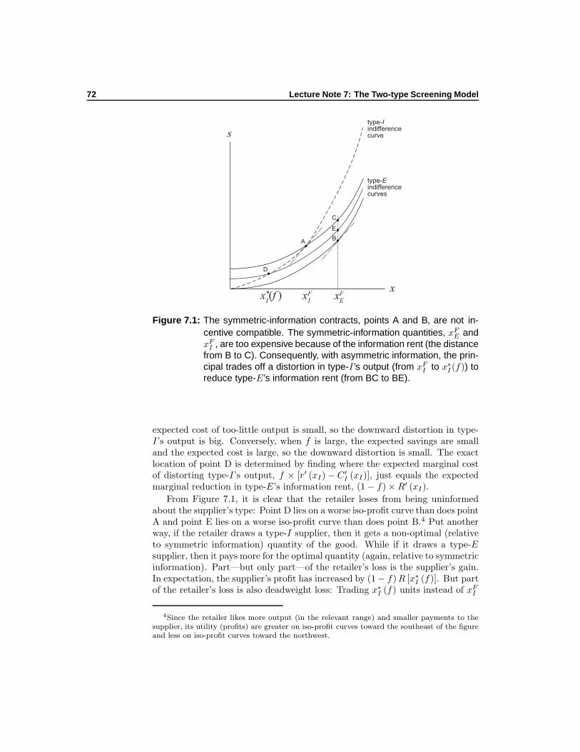
72 Lecture Note 7: The Two-type Screening Model
x
s
A
C
B
E
D
type-Iindifferencecurve
type-Eindifferencecurves
FIx xF
E*Ix (f )
Figure 7.1: The symmetric-information contracts, points A and B, are not in-centive compatible. The symmetric-information quantities, xFE andxFI , are too expensive because of the information rent (the distancefrom B to C). Consequently, with asymmetric information, the prin-cipal trades off a distortion in type-I ’s output (from xFI to x∗I(f)) toreduce type-E’s information rent (from BC to BE).
expected cost of too-little output is small, so the downward distortion in type-I’s output is big. Conversely, when f is large, the expected savings are smalland the expected cost is large, so the downward distortion is small. The exactlocation of point D is determined by finding where the expected marginal costof distorting type-I’s output, f × [r′ (xI) − C′
I (xI)], just equals the expectedmarginal reduction in type-E’s information rent, (1 − f) ×R′ (xI).
From Figure 7.1, it is clear that the retailer loses from being uninformedabout the supplier’s type: Point D lies on a worse iso-profit curve than does pointA and point E lies on a worse iso-profit curve than does point B.4 Put anotherway, if the retailer draws a type-I supplier, then it gets a non-optimal (relativeto symmetric information) quantity of the good. While if it draws a type-Esupplier, then it pays more for the optimal quantity (again, relative to symmetricinformation). Part—but only part—of the retailer’s loss is the supplier’s gain.In expectation, the supplier’s profit has increased by (1 − f)R [x∗I (f)]. But partof the retailer’s loss is also deadweight loss: Trading x∗I (f) units instead of xFI
4Since the retailer likes more output (in the relevant range) and smaller payments to thesupplier, its utility (profits) are greater on iso-profit curves toward the southeast of the figureand less on iso-profit curves toward the northwest.
7.2 Contracts under Incomplete Information 73
units is simply inefficient. In essence, our retailer is a monopsonist and, as istypical of monopsony, there is a deadweight loss.5 Moreover, the deadweightloss arises here for precisely the same reason it occurs in monopsony: Like amonopsonist, our retailer is asking the payment (price) schedule to play tworoles. First, it asking it to allocate goods and, second, it is asking it to preserveits rents from having all the bargaining power. Since only the first role hasanything to do with allocative efficiency, giving weight to the second role canonly create allocative inefficiency. As often happens in economics, a decisionmaker has one instrument—here, the payment schedule—but is asking it toserve multiple roles. Not surprisingly then, the ultimate outcome is less thanfirst best (recall our discussion of the two-instruments principle page 28).
Because the first best is not achieved, it is natural to ask whether the retailercould improve on the outcome in Proposition 10 by using some more sophisti-cated contract? The answer is no and the proof is, as we will see later, quitegeneral. Whatever sophisticated contract the retailer uses, this contract willboil down to a pair of points, (xI , sI) and (xE , sE), once it is executed; that is,a final quantity traded and a final payment for each possible state of nature.Consequently, whatever complicated play is induced by the contract, both par-ties can see through it and forecast that the equilibrium outcomes correspond tothese two points. Moreover, by mimicking the strategy it would play in state t,the supplier can generate either of the two outcomes regardless of the true state.In addition, if it can’t profit from (xt, st) in state t, it can simply not participate.Necessary equilibrium conditions are, then, that the supplier choose (xt, st) instate t rather than (xt′ , st′), t 6= t′, and that it choose to participate anticipat-ing that it will choose (xt, st) in state t. But these are precisely the revelationand participation constraints (7.2), (7.3), (7.6), and (7.7). Therefore, whateverthe contractual arrangement, the final outcome can always be generated by asimple (non-linear) payment schedule like the one derived above. We’ve, thus,established that the outcome described in Proposition 10 cannot be improvedon by using more sophisticated or alternative contracts.6
Finally, note that we don’t need an entire payment schedule, S (·). In partic-ular, there is a well-known alternative: a direct-revelation contract (mechanism).In a direct-revelation contract, the retailer commits to pay the supplier sE forxE or sI for xI depending on the supplier’s announcement of its type. Failureby the supplier to announce its type (i.e., failure to announce a t ∈ E, I) isequivalent to the supplier rejecting the contract. Finally, if, after announcingits type, the supplier produces a quantity other than xt, the supplier is pun-ished (e.g., paid nothing). It is immediate that this direct-revelation contract isequivalent to the optimal payment schedule derived above. It is also simpler, in
5Monopsony is a situation in which the buyer has all the market power (in contrast tomonopoly, in which the seller has all the market power).
6This is not to say that another contract couldn’t do as well. This is rather obvious: Forinstance, suppose S (x) = 0 for all x except xE and xI , where it equals sE or sI , respectively.We’ve merely established that no other contract can do strictly better than the S (·) derivedin the text.
74 Lecture Note 7: The Two-type Screening Model
that it only deals with the relevant part of the payment schedule. Admittedly,it is not terribly realistic,7 but as this discussion suggests we can transform adirect-revelation contract into a more realistic contract (indeed, we will formal-ize this below in Proposition 12). More importantly, as we will see, in terms ofdetermining what is the optimal feasible outcome, there is no loss of generalityin restricting attention to direct-revelation contracts.
7Although see Gonik (1978) for a real-life example of a direct-revelation mechanism.
General ScreeningFramework 8
The two-type screening model yielded strong results. But buried within it is alot of structure and some restrictive assumptions. If we are really to use thescreening model to understand economic relationships, we need to deepen ourunderstanding of the phenomena it unveils, the assumptions they require, andthe robustness of its conclusions. Our approach in this section is, thus, to startfrom a very general formalization of the problem and to motivate or discuss theassumptions necessary for making this model “work.”
A principal and an agent are involved in a relationship that can be charac-terized by an allocation x ∈ X and a real-valued monetary transfer s ∈ S ⊂ R
between the two players. A transfer-allocation pair, (x, s), is called an outcome.The space of possible allocations, X , can be quite general: Typically, as in ouranalysis of the retailer-supplier problem, it’s a subspace of R; but it could beanother space, even a multi-dimensional one. In what follows, we assume thatoutcomes are verifiable.
The agent’s information is characterized by a parameter θ ∈ Θ. As before,we’ll refer to this information as the agent’s type. The type space, Θ, canbe very general. Typically, however, it is either a discrete set (e.g., as in theretailer-supplier example where we had Θ = I, E) or a compact interval in R.Nature draws θ from Θ according to a commonly known probability distribution.While the agent learns the value of θ perfectly, the principal only knows that itwas drawn from the commonly known probability distribution.
Both players’ preferences are described by von Neumann-Morgenstern utilityfunctions, W(x, s, θ) for the principal and U(x, s, θ) for the agent, where bothare defined over X ×S×Θ. Because we interpret s as a transfer from theprincipal to the agent, we assume that U increases in s, while W decreases in s.For convenience, we assume these utility functions are smooth; more precisely,that they are three-times continuously differentiable.1
To have a fully general treatment, we need to extend this analysis to allowfor the possibility that the actual outcome is chosen randomly from X ×S. Tothis end, let σ denote a generic element of the set of probability distributions,∆(X ×S
), over the set of possible outcomes, X ×S. We extend the utility
functions to ∆(X ×S
)through the expectation operator:
W(σ, θ) ≡ Eσ [W(x, s, θ)] and U(σ, θ) ≡ Eσ [U(x, s, θ)] .
1One could relax this smoothness assumption, but the economic value of doing so is toosmall to warrant time on this issue.
75
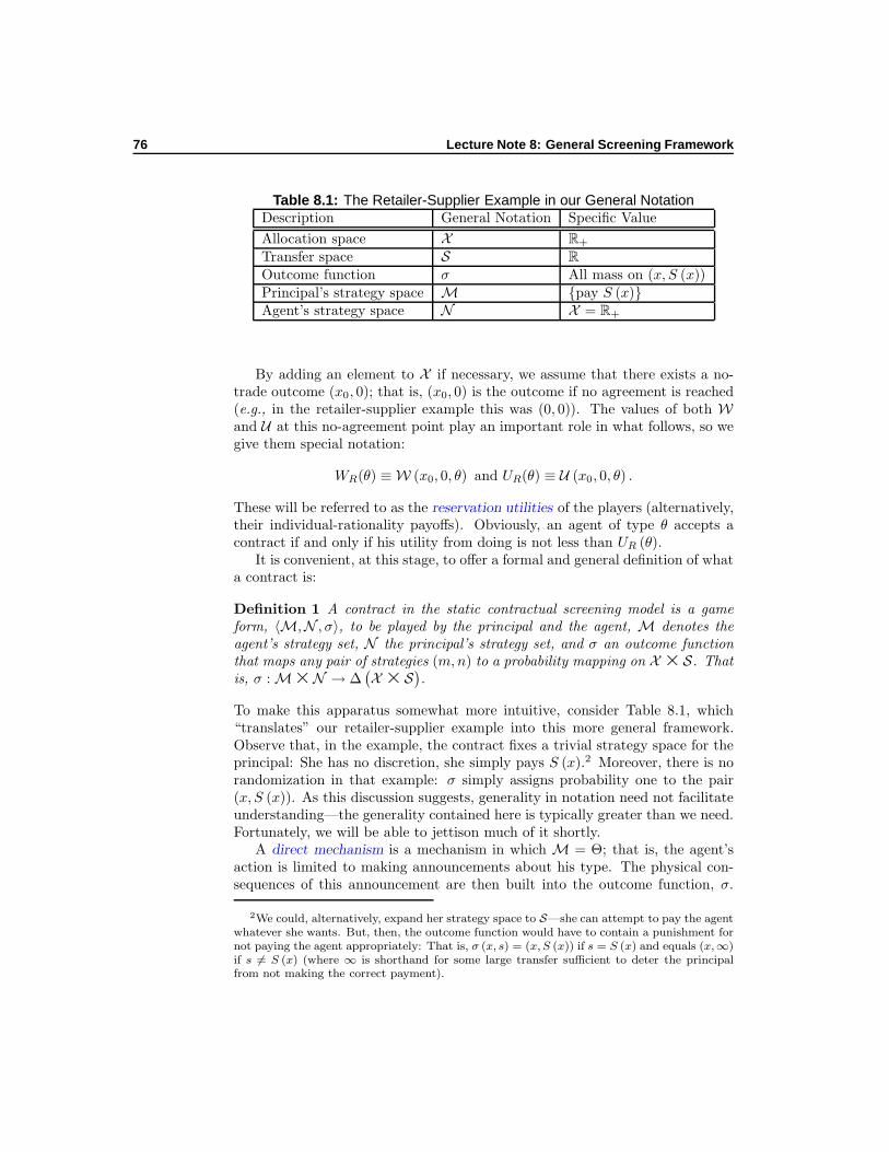
76 Lecture Note 8: General Screening Framework
Table 8.1: The Retailer-Supplier Example in our General NotationDescription General Notation Specific Value
Allocation space X R+
Transfer space S R
Outcome function σ All mass on (x, S (x))Principal’s strategy space M pay S (x)Agent’s strategy space N X = R+
By adding an element to X if necessary, we assume that there exists a no-trade outcome (x0, 0); that is, (x0, 0) is the outcome if no agreement is reached(e.g., in the retailer-supplier example this was (0, 0)). The values of both Wand U at this no-agreement point play an important role in what follows, so wegive them special notation:
WR(θ) ≡ W (x0, 0, θ) and UR(θ) ≡ U (x0, 0, θ) .
These will be referred to as the reservation utilities of the players (alternatively,their individual-rationality payoffs). Obviously, an agent of type θ accepts acontract if and only if his utility from doing is not less than UR (θ).
It is convenient, at this stage, to offer a formal and general definition of whata contract is:
Definition 1 A contract in the static contractual screening model is a gameform, 〈M,N , σ〉, to be played by the principal and the agent, M denotes theagent’s strategy set, N the principal’s strategy set, and σ an outcome functionthat maps any pair of strategies (m,n) to a probability mapping on X ×S. Thatis, σ : M×N → ∆
(X ×S
).
To make this apparatus somewhat more intuitive, consider Table 8.1, which“translates” our retailer-supplier example into this more general framework.Observe that, in the example, the contract fixes a trivial strategy space for theprincipal: She has no discretion, she simply pays S (x).2 Moreover, there is norandomization in that example: σ simply assigns probability one to the pair(x, S (x)). As this discussion suggests, generality in notation need not facilitateunderstanding—the generality contained here is typically greater than we need.Fortunately, we will be able to jettison much of it shortly.
A direct mechanism is a mechanism in which M = Θ; that is, the agent’saction is limited to making announcements about his type. The physical con-sequences of this announcement are then built into the outcome function, σ.
2We could, alternatively, expand her strategy space to S—she can attempt to pay the agentwhatever she wants. But, then, the outcome function would have to contain a punishment fornot paying the agent appropriately: That is, σ (x, s) = (x, S (x)) if s = S (x) and equals (x,∞)if s 6= S (x) (where ∞ is shorthand for some large transfer sufficient to deter the principalfrom not making the correct payment).

77
For instance, as we saw at the end of the previous section, we can translateour retailer-supplier contract into a direct mechanism: M = E, I, N is asingleton (so we can drop n as an argument of σ), and
σ (m) =
(xI , sI) = (x∗I (f) , CI [x∗I (f)]) if m = I(xE , sE) =
(xFE , R [x∗I (f)] + CE
(xFE))
if m = E.
A direct-revelation mechanism (alternatively, a direct truthful mechanism) is adirect mechanism where it is an equilibrium strategy for the agent to tell thetruth: Hence, if m (·) : Θ → Θ is the agent’s strategy, we have m(θ) = θ inequilibrium for all θ ∈ Θ. That is, for any θ and θ′ in Θ,
U(σ (m [θ]) , θ) ≥ U (σ (m [θ′]) , θ) .
Note that not every direct mechanism will be a direct-revelation mechanism.Being truthful in equilibrium is a property of a mechanism; that is, it dependson σ (·).
Observe that the design of a contract means choosing M, N , and σ. Intheory, the class of spaces and outcome functions is incomprehensibly large.How can we find the optimal contract in such a large class? Indeed, given theinherent difficulties in even characterizing such a large class, how can we everbe sure that we’ve found the optimal contract? Fortunately, two simple, yetsubtle, results—the revelation principle and the the taxation principle—allowus to avoid these difficulties.3 From the revelation principle, the search for onoptimal contract reduces without loss of generality to the search for the optimaldirect-revelation mechanism. Moreover, if the outcome in the direct-revelationmechanism is a deterministic function of the agent’s announcement, then, fromthe taxation principle, we may further restrict attention to a payment schedulethat is a function of the allocation x (as we did in the retailer-supplier example).
Proposition 11 (The Revelation Principle)4 For any general contract (M,N , σ) and associated Bayesian equilibrium, there exists a direct-revelation mech-anism such that the associated truthful Bayesian equilibrium generates the sameequilibrium outcome as the general contract.
Proof: The proof of the revelation principle is standard but informative. ABayesian equilibrium of the game (M,N , σ) is a pair of strategies (m(·), n).5
Let us consider the following direct mechanism: σ(·) = σ(m(·), n). Our claim is
3It is unfortunate that these two fundamental results are called principles, since theyare not, as their names might suggest, premises or hypotheses. They are, as we will show,deductive results.
4The revelation principle is often attributed to Myerson (1979), although Gibbard (1973)and Green and Laffont (1977) could be identified as earlier derivations. Suffice it to saythat the revelation principle has been independently derived a number of times and was awell-known result before it received its name.
5Observe that the agent’s strategy can be conditioned on θ, which he knows, while theprincipal’s cannot be (since she is ignorant of θ).
78 Lecture Note 8: General Screening Framework
that σ (·) induces truth-telling (is a direct-revelation mechanism). To see this,suppose it were not true. Then there must exist a type θ such that the agentdoes better to lie—announce some θ′ 6= θ—when he is type θ. Formally, theremust exist θ and θ′ 6= θ such that
U(σ(θ′), θ) > U(σ(θ), θ).
Using the definition of σ(·), this means that
U(σ [m(θ′), n] , θ) > U(σ [m (θ) , n] , θ);
but this means the agent prefers to play m(θ′) instead of m(θ) in the originalmechanism against the principal’s equilibrium strategy n. This, however, can’tbe since m(·) is an equilibrium best response to n in the original game. Hence,truthful revelation must be an optimal strategy for the agent under the con-structed direct mechanism. Finally, when the agent truthfully reports the stateof nature in the direct truthful mechanism, the same outcome σ(θ) = σ(m(θ), n)is implemented in equilibrium.
An intuitive way to see the revelation principle is imagine that before heplays some general mechanism, the agent could delegate his play to some trust-worthy third party. There are two equivalent ways this delegation could work.One, the agent could tell the third party to play m. Alternatively, if the thirdparty knows the agent’s equilibrium strategy—the mapping m : Θ → M—then the agent could simply reveal (announce) his type to the third party withthe understanding that the third party would choose the appropriate actions,m (θ). But, because we can build this third party into the design of our direct-revelation mechanism, this equivalence means that there is no loss of generalityin restricting attention to direct-revelation mechanisms.
The taxation principle requires a little more structure: It assumes that thereis a possibility of punishing the agent so as to deter him from violating thecontractual rules
Assumption 2 (Existence of a punishment) There exists an s ∈ R suchthat:
sup(x,θ)∈X×Θ
U(x, s, θ) ≤ inf(x,s,θ)∈X×S×Θ
U(x, s, θ).
In other words, there exists a punishment so severe that the agent would alwaysprefer not to suffer it.
With this assumption, one can construct a payment schedule that gener-ates the same outcome as any deterministic direct-revelation mechanism and is,therefore, as general as any contract in this context.
Proposition 12 (The Taxation Principle) Under Assumption 2, the equi-librium outcome under any deterministic direct-revelation mechanism, σ (·) =
79
(x(·), s (·)), is also an equilibrium outcome of the game where the principal pro-poses the payment schedule S(·) defined by
S(x) =
s(θ) , if θ ∈ x−1(x) (i.e., such that x = x(θ) for some θ ∈ Θ)s, otherwise
.
Proof: Let’s first establish that S (·) is unambiguously defined: Suppose thereexisted θ1 and θ2 such that
x = x(θ1) = x(θ2),
but s(θ1) 6= s(θ2). We’re then free to suppose that s(θ1) > s(θ2). Then, becauseU is increasing in s,
U(x(θ1), s(θ1), θ2) > U(x(θ2), s(θ2), θ2).
But this means the agent would prefer pretending that the state of natureis θ2 when it’s actually θ1; the mechanism would not be truthful. Hence, ifθ1, θ2 ∈ x−1 (x), we must have s (θ1) = s (θ2); that is, the payment scheduleS(·) is unambiguously defined.
Now, the agent’s problem when faced with the payment schedule S(·) is sim-ply to choose the allocation x that maximizes U(x, S(x), θ). Given the severityof the punishment, the agent will restrict his choice to x ∈ x(Θ). But since ouroriginal mechanism was a direct-revelation mechanism, we know
U (x (θ) , s (θ) , θ) ≥ U (x (θ′) , s (θ′) , θ)
for all θ and θ′. So no type θ can do better than to choose x = x (θ).
The economic meaning of the taxation principle is straightforward: Whendesigning a contract, the principal is effectively free to focus on “realistic” com-pensation mechanisms that pay the agent according to his achievements. Hence,as we argued above, there is no loss of generality in our solution to the retailer-supplier problem.
Although payment schedules involve no loss of generality and are realistic,they are often nonlinear, which creates difficulties in working with them.6 Inparticular, when looking for the optimal non-linear price schedule, one mustbe able to compute the functional mapping that associates to each scheduleS(·) the action choice x(θ) that maximizes U(x, S(x), θ). Even assuming S (·)is differentiable—which is not ideal because one should refrain from making as-sumptions about endogenous variables—solving this problem can be difficult.Direct-revelation mechanisms, on the other hand, allow an easier mathemati-cal treatment of the problem using standard convex analysis: The revelationconstraints simply consist of writing θ′ = θ is a maximum of U(x(θ′), s(θ′), θ)
6Admittedly, if the derived payment schedule is sufficiently nonlinear, one could begin toquestion its realism, as real-world contracts are often linear or, at worst, piecewise linear.Although see footnote 7 on page 74 for an example of where reality “matches” theory.

80 Lecture Note 8: General Screening Framework
and writing that a given point is a maximum is easier that characterizing anunknown maximum. For this reason, much of the mechanism-design literaturehas focussed on direct-revelation mechanisms over optimal-payment schedulesdespite the latter’s greater realism.
The StandardFramework 9
As we’ve already hinted, the general framework introduced in the previous sec-tion is more general than what is commonly used. In this section, we willtherefore considered a restricted framework known as the “standard” frame-work, Much of the contractual screening literature can be placed within thisstandard framework. We begin by defining this framework and contrasting it tothe more general framework introduced above. At the end of this note, I offerless conventional views on the screening model, which require departing fromthe standard framework. In order to provide a road map to the reader, I spellout each assumption in this section and suggest what consequences would arisefrom alternative assumptions.
In the standard framework, the allocation space, X , is R+.1 The type space,Θ, is [θL, θH ] ⊂ R, where both bounds, θL and θH , are finite.2 The most criticalassumptions in going from the general framework to the standard framework in-volve the utility functions. Henceforth, we assume they are additively separablein the transfer and the allocation. Moreover, we assume the marginal value ofmoney is type independent (i.e., ∂ (∂U/∂s) /∂θ = ∂ (∂W/∂s) /∂θ = 0). Theseassumptions simplify the analysis by eliminating income effects from consider-ation. Formally, the agent’s and principal’s utility functions are
U(x, s, θ) = s+ u(x, θ) and
W(x, s, θ) = w(x, θ) − s,
respectively. Essentially for convenience, we take u(·, ·) and w (·, ·) to be three-times continuously differentiable. The aggregate (full-information) surplus isdefined as:
Ω(x, θ) = w(x, θ) + u(x, θ).
We also assume, mainly for convenience, that
1. Some trade is desirable: For all θ ∈ (θL, θH ], ∂Ω (0, θ) /∂x > 0.
2. There can be too much of a good thing: For all θ ∈ [θL, θH ] ∃x (θ)such that Ω (x, θ) ≤ Ω (0, θ) for all x > x (θ).
1That the space be bounded below at 0 is not critical—any lower bound would do. Alter-natively, by appropriate changes to the utility functions, we could allow the allocation spaceto be unbounded. Zero is simply a convenience.
2This constitutes no loss of economic (as opposed to mathematical) generality, since wecan set the bounds as far apart as we need.
81
82 Lecture Note 9: The Standard Framework
Observe these two assumptions entail that Ω (x, θ) has an interior maximum forall θ ∈ (θL, θH ]. If the first assumption didn’t hold for at least some types, thentrade—contracting—would be pointless. Extending the desirability of trade toalmost all types saves from the bookkeeping headache of distinguishing betweentypes with which trade is efficient and those with which it is not. The secondassumption is just one of many ways of expressing the sensible economic ideathat, beyond some point, welfare is reduced by trading more.
Observe that the standard framework is restrictive in several potential im-portant ways:
• The type space is restricted to be one-dimensional. In many applica-tions, such as the retailer-supplier example, this is a natural assumption.One can, however, conceive of applications where it doesn’t fit: Suppose,e.g., the retailer cared about the quantity and quality of the goods re-ceived and the supplier’s type varied on both an efficiency dimension anda conscientiousness-of-employees dimension (the latter affecting the costof providing quality). Not surprisingly, restricting attention to one di-mension is done for analytic tractability: Assuming a single dimensionmake the order properties of the type space straightforward (i.e., greaterand less than are well-defined on the real line). As we will see, the orderproperties of the type space are critical to our analysis.
• The set of possible allocations is one-dimensional. Again, this is sufficientfor some applications (e.g., the quantity supplied to the retailer), but notothers (e.g., when the retailer cares about both quantity and quality).The difficulty in expanding to more than one dimension arise from diffi-culties in capturing how the agent’s willingness to make tradeoffs amongthe dimensions (including his income) varies with his type. The readerinterested in this extension should consult Rochet and Chone (1998).
• As noted, the utility functions are separable in money and allocation; themarginal utility of income is independent of the state of nature; and themarginal utility of income is constant, which means both players are riskneutral with respect to gambles over money. The gains from these as-sumptions are that we can compute the transfer function s(·) in terms ofthe allocation function x(·), which means our optimization problem is astandard optimal-control problem with a unique control, x(·). In addition,risk neutrality insulates us from problems that exogenously imposed riskmight otherwise create (e.g., the need to worry about mutual insurance).On the other hand, when the agent is risk averse, the ability to threatenhim with endogenously imposed risk (from the contract itself) can providethe principal an additional tool with which to improve the ultimate allo-cation. For a discussion of some of these issues see Edlin and Hermalin(2000). Note we still have the flexibility to endogenously impose risk overthe allocation (the x), we discuss the desirability of doing so below. Seealso Maskin (1981).

83
Continuing with our development of the standard framework, we assumethat nature chooses the agent’s type, θ, according to the distribution functionF (·) : [θL, θH ] → [0, 1]. Let f (·) be the associated density function, whichwe assume to be continuous and to have full support (i.e., f (θ) > 0 for allθ ∈ [θL, θH ]). Assuming a continuum of types and a distribution without masspoints is done largely for convenience. It also generalizes our analysis from justtwo types. Admittedly, we could have generalized beyond two types by allowingfor a finite number of types greater than two. The conclusions we would reachby doing so would be economically similar to those we’ll shortly obtain with acontinuum of types.3 The benefit of going all the way to the continuum is itallows us to employ calculus, which streamlines the analysis.
Recall that, at its most general, a direct-revelation mechanism is a mapping from the type space into a distribution over outcomes. Given the way thatmoney enters both players utility functions, we’re free to replace a distributionover payments with an expected payment, which means we’re free to assumethat the payment is fixed deterministically by the agent’s announcement.4 Whatabout random-allocation mechanisms? The answer depends on the risk proper-ties of the two players’ utilities over allocation. If we postulate that w (·, θ) andu (·, θ) are concave for all θ ∈ [θL, θH ], then, absent incentive concerns, therewould be no reason for the principal to prefer a random-allocation mechanism;indeed, if at least one is strictly concave (i.e., concave, but not affine), thenshe would strictly prefer not to employ a random-allocation mechanism absentincentive concerns: Her expected utility is greater with a deterministic mecha-nism and, since the agent’s expected utility is greater, her payment to him willbe less (a benefit to her). Hence, we would only expect to see random-allocationmechanisms if the randomness somehow relaxed the incentive concerns. Wheredoes this leave us? At this point, consistent with what is standardly done, wewill assume that both w (·, θ) and u (·, θ) are concave, with one at least beingstrictly concave, for all θ ∈ [θL, θH ] (note this entails that Ω (·, θ), the socialsurplus function, is also strictly concave). Hence, absent incentive concerns,we’d be free to ignore random-allocation mechanisms. For the time being, we’llalso ignore random-allocation mechanisms with incentive concerns. Later, we’llconsider the circumstances under which this is appropriate. Since we’re ignoringrandom mechanisms, we’ll henceforth write 〈x(·), s(·)〉 instead of σ (·) for themechanism.
Within this framework, the route that we follow consists of two steps. First,we will characterize the set of direct-revelation contracts; that is, the set of con-tracts 〈x(·), s(·)〉 from [θL, θH ] to R × R+ that satisfy truthful revelation. Thistruthful-revelation—or incentive compatibility—condition can be expressed as:
s(θ) + u(x(θ), θ
)≥ s(θ) + u
(x(θ), θ
)(9.1)
3See, e.g., Caillaud and Hermalin (1993), particular §3, for a finite-type-space analysisunder the standard framework.
4That is, the mechanism that maps θ to a distribution G (θ) over payments is equivalentto a mechanism that maps θ to the deterministic payment s (θ) = EG(θ) s.
84 Lecture Note 9: The Standard Framework
for all (θ, θ) ∈ [θL, θH ]2. After completing this first step, the second step isidentifying from within this set of incentive-compatible contracts the one thatmaximizes the principal’s expected utility subject to the agent’s participation.Whether the agent participates depends on whether his equilibrium utility ex-ceeds his reservation utility, UR(θ). Observe that the requirement that theagent accept the contract imposes an additional constraint on the principalin designing the optimal contract. As before, we refer to this constraint asthe participation or individual-rationality (ir) constraint. Recall that X is as-sumed to contain a no-trade allocation, x0, s = 0 is a feasible transfer, andUR (θ) ≡ U (x0, 0, θ). Hence there is no loss of generality in requiring the prin-cipal to offer a contract that is individually rational for all types (although the“contract” for some types might be no trade).
We assume that the agent acts in the principal’s interest when he’s otherwiseindifferent. In particular, he accepts a contract when he is indifferent betweenaccepting and rejecting it and he tells the truth when indifferent between beinghonest and lying. This is simply a necessary condition for an equilibrium toexist and, as such, should not be deemed controversial.
In our treatment of the retailer-supplier example, we assumed that bothtypes of supplier had the same reservation utility (i.e., recall, UR(θ) = U(0, 0, θ)= −Cθ(0) = 0). It is possible, however, to imagine models in which the reser-vation utility varies with θ. For instance, suppose that an efficient suppliercould, if not employed by the retailer, market its goods directly to the ultimateconsumers (although, presumably, not as well as the retailer could). Suppose,in fact, it would earn a profit of πE > 0 from direct marketing. Then wewould have UR (E) = πE and UR (I) = 0. A number of authors (see, e.g.,Lewis and Sappington, 1989, Maggi and Rodriguez-Clare, 1995, and Jullien,1996) have studied the role of such type-dependent reservation utilities in con-tractual screening models. Type dependence can, however, greatly complicatethe analysis. We will, therefore, adopt the more standard assumption of type-independent reservation utilities; that is, we assume—as we did in our retailer-supplier example—that
UR(θ) = UR and WR(θ) = WR
for all θ ∈ [θL, θH ]. As a further convenience, we will interpret x = 0 as theno-trade allocation. Observe that these last two assumptions imply
u (0, θ) = u (0, θ′) = UR and
w (0, θ) = w (0, θ′) = WR
for all θ, θ′ ∈ [θL, θH ]. Given these assumptions, we can express the agent’sparticipation constraint as
s (θ) + u(x(θ), θ
)≥ UR. (9.2)
Although our treatment of reservation utilities and no trade is standard, wehave, nevertheless added to the assumptions underlying the standard framework.

9.1 The Spence-Mirrlees Assumption 85
At last, we can state the problem that we seek to solve: Find the optimalcontract 〈x (·) , s (·)〉 that maximizes
∫ θH
θL
(w(x(θ), θ
)− s(θ)
)f(θ)dθ (9.3)
subject to (9.1) and (9.2) holding.Before solving this program, it’s valuable to consider the full (symmetric)
information benchmark: Ex post efficiency corresponds to adopting the alloca-tion
xF (θ) ∈ arg maxx∈R+
Ω(x, θ)
for each θ (recall Ω(x, θ) is the aggregate surplus from the relationship). Ourearlier assumptions ensure that Ω(·, θ) is strictly concave for each θ; so the expost efficient allocation is uniquely defined by the first-order condition:
∂Ω
∂x(xF (θ), θ) =
∂w
∂x(xF (θ), θ) +
∂u
∂x(xF (θ), θ) = 0.
Our earlier assumptions also entail that xF (·) is uniformly bounded from above.Observe that any sharing of the surplus can, then, be realized by the appropriatetransfer function.5 It follows that, if the principal knows θ—that is, the partiesare playing under full (symmetric) information—then the contracting game canbe easily solved: In equilibrium, the principal offers a contract
⟨xF (·), sF (·)
⟩
such that the agent’s utility is exactly equal to his reservation utility; that is,
sF (θ) = UR − u(xF (θ), θ).
In other words, the principal captures the entire surplus—a consequence ofendowing her with all the bargaining power—leaving the agent at his outside(non-participation) option.
The Spence-MirrleesAssumption 9.1
Before we proceed to solve (9.3), we need to introduce one more assumption.Given this assumption’s importance, it is worth devoting a short section to it.
In order to screen types, the principal must be able to exploit differencesacross the tradeoffs that different types are willing to make between money andallocation. Otherwise a strategy, for instance, of decreasing the x expected fromthe agent in exchange for slightly less pay wouldn’t work to induce one type toreveal himself to be different than another type. Recall, for instance, becausethe marginal cost of output differed between the efficient and inefficient types
5Note that this is an instance of where we’re exploiting the additive separability (lack ofincome effects) assumed of the utility functions. Were there income effects, we couldn’t definexF (·) independently of the transfers.
86 Lecture Note 9: The Standard Framework
in our retailer-supplier example, the buyer could design a contract to inducerevelation. Different willingness to make tradeoffs means we require that theindifference curves of the agent in x-s space differ with his type. In fact, wewant, for any point in x-s space, that these slopes vary monotonically withwhatever natural order applies to the type space. Or, when, no natural orderapplies, we want it to be possible to define an order, ≻, over the types so thatθ ≻ θ′ if and only if the slope of θ’s indifference curve is greater (alternativelyless) than the slope of θ′’s indifference at every point (x, s) ∈ X × S. Sucha monotonicity-of-indifference-curves condition is known as a Spence-Mirrleescondition and, correspondingly, the assumption that this condition is met isknown as the Spence-Mirrlees assumption.
The slope of the indifference curve in x-s space is equal to −∂u/∂x. Hence,we require that −∂u/∂x or, equivalently and more naturally, ∂u/∂x vary mono-tonically in θ. Specifically, we assume:
Assumption 3 (Spence-Mirrlees) For all x ∈ X ,
∂u (x, θ)
∂x>∂u (x, θ′)
∂x
if θ > θ′.
That is, if θ > θ′—θ is a higher type than θ′—then −1 times the slope of typeθ’s indifference curve is, at any point, greater than −1 times the slope of typeθ′’s indifference curve. Observe that a consequence of Assumption 3 is thata given indifference curve for one type can cross a given indifference curve ofanother type at most once. For this reason, the Spence-Mirrlees Assumption issometimes called a single-crossing condition. Figure 9.1 illustrates.
Lemma 7 Assuming (as we are) that u(·, ·) is at least twice differentiable inboth arguments, then the Spence-Mirrlees assumption (Assumption refass:S-M1)is equivalent to assuming
∂2u(x, θ)
∂θ∂x> 0 . (9.4)
Proof: As a differentiable function cannot be everywhere increasing unless itsderivative is positive, the fact that the Spence-Mirrlees assumption implies (9.4)is obvious. To go the other way, observe (9.4) implies
0 <
∫ θ
θ′
∂2u(x, t)
∂θ∂xdt
= u(x, θ) − u(x, θ′) , (9.5)
where (9.5) follows from the fundamental theorem of calculus.
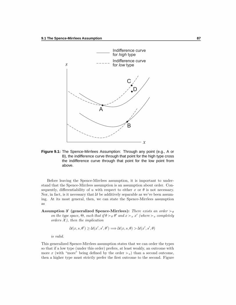
9.1 The Spence-Mirrlees Assumption 87
s
x
A
B
C
Indifference curvefor high type
Indifference curvefor low type
D
Figure 9.1: The Spence-Mirrlees Assumption: Through any point (e.g., A orB), the indifference curve through that point for the high type crossthe indifference curve through that point for the low point fromabove.
Before leaving the Spence-Mirrlees assumption, it is important to under-stand that the Spence-Mirrlees assumption is an assumption about order. Con-sequently, differentiability of u with respect to either x or θ is not necessary.Nor, in fact, is it necessary that U be additively separable as we’ve been assum-ing. At its most general, then, we can state the Spence-Mirrlees assumptionas
Assumption 3′ (generalized Spence-Mirrlees): There exists an order ≻θon the type space, Θ, such that if θ ≻θ θ′ and x ≻x x′ (where ≻x completelyorders X ), then the implication
U(x, s, θ′) ≥ U(x′, s′, θ′) =⇒ U(x, s, θ) > U(x′, s′, θ)
is valid.
This generalized Spence-Mirrlees assumption states that we can order the typesso that if a low type (under this order) prefers, at least weakly, an outcome withmore x (with “more” being defined by the order ≻x) than a second outcome,then a higher type must strictly prefer the first outcome to the second. Figure
88 Lecture Note 9: The Standard Framework
9.1 illustrates: Since the low type prefers point C to A (weakly), the hightype must strictly prefer C to A, which the figure confirms. Similarly, sincethe low type prefers C to B (strictly), the high type must also strictly preferC to B, which the figure likewise confirms. See Milgrom and Shannon (1994)for a more complete discussion of the relationship between Assumption 3 andAssumption 3′.
As suggested at beginning of this section, a consequence of the Spence-Mirrlees assumption is that it is possible to separate any two types; by whichwe mean it is possible to find two outcomes (x1, s1) and (x2, s2) such that atype-θ1 agent prefers (x1, s1) to (x2, s2), but a type-θ2 agent has the oppositepreferences. For instance, in Figure 9.1, let point A be (x1, s1) and let D be(x2, s2). If θ2 is the high type and θ1 is the low type, then it is clear that giventhe choice between A and D, θ1 would select A and θ2 would select D; that is,this pair of contracts separates the two types. Or, for example, back in Figure7.1, contracts D and E separate the inefficient and efficient types of supplier.
Characterizing theIncentive-Compatible
Contracts 9.2Our approach to solving the principal’s problem (9.3) is a two-step one. First,we will find a convenient characterization of the set of incentive-compatiblemechanisms (i.e., those that satisfy (9.1)). This is our objective here. Later, wewill search from within this set for those that maximize (9.3) subject to (9.2).
Within the standard framework it is relatively straightforward to derive thenecessary conditions implied by the self-selection constraints. Our approachis standard (see, e.g., Myerson, 1979, among others). Consider any direct-revelation mechanism 〈x (·) , s (·)〉 and consider any pair of types, θ1 and θ2,with θ1 < θ2. Direct revelation implies, among other things, that type θ1 won’twish to pretend to be type θ2 and vice versa. Hence,
s(θ1) + u [x(θ1), θ1] ≥ s(θ2) + u [x(θ2), θ1] and
s(θ2) + u [x(θ2), θ2] ≥ s(θ1) + u [x(θ1), θ2] .
As is often the case in this literature, it is easier to work with utilities thanpayments. To this end, define
v(θ) = s(θ) + u [x(θ), θ] .
Observe that v (θ) is the type-θ agent’s equilibrium utility. The above pair ofinequalities can then be written as:
v (θ1) ≥ v (θ2) − u [x (θ2) , θ2] + u [x (θ2) , θ1] and
v (θ2) ≥ v (θ1) − u [x(θ1), θ1] + u [x(θ1), θ2] .
9.2 Characterizing the Incentive-Compatible Contracts 89
Or, combining these two inequalities, as
∫ θ2
θ1
∂u [x(θ1), θ]
∂θdθ ≤ v(θ2) − v(θ1) ≤
∫ θ2
θ1
∂u [x(θ2), θ]
∂θdθ. (9.6)
This double inequality has two consequences. First, ignoring the middleterm, it implies
∫ θ2
θ1
∫ x(θ2)
x(θ1)
∂2u
∂x∂θ(x, θ)dxdθ ≥ 0.
The Spence-Mirrlees assumption means the integrand is positive. Given θ1 < θ2,this means the integral can be non-negative only if x(θ1) ≤ x(θ2). Since this istrue for any θ1 < θ2, we may conclude that the allocation function x(·) is non-decreasing. Note that this necessarily implies that x(·) is almost everywherecontinuous.
The second consequence of (9.6) is as follows: By fixing one end point andletting the other converge towards it, we see that v(·) is absolutely continuouswith respect to Lebesgue measure and is, thus, almost everywhere differen-tiable.6 This derivative is
dv (θ)
dθ=∂u(x(θ), θ)
∂θ
almost everywhere.7 Consequently, one can express equilibrium utility as
v(θ) = v(θL) +
∫ θ
θL
∂u
∂θ(x(t), t)dt. (9.7)
Expression (9.7) and the monotonicity of the allocation function x(·) are,thus, necessary properties of a direct-revelation mechanism. In particular, we’vejust proved that a necessary condition for an allocation function x (·) to beimplementable is that
s(θ) = vL − u(x(θ), θ) +
∫ θ
θL
∂u
∂θ(x(t), t)dt.
where vL is an arbitrary constant.
It turns out that these properties are also sufficient :
6To be precise, one should make assumptions to ensure that ∂u(x(·), ·)/∂θ is integrable onΘ. This can be done by requiring that X be bounded or that ∂u(·, ·)/∂θ be bounded on X ×Θ.Both assumptions are natural in most economic settings and simply extend the assumptionsthat bound xF (·). Henceforth, we assume ∂u/∂θ is bounded.
7Note the important difference between∂u[x(θ),θ]
∂θand
du[x(θ),θ]dθ
. The former is the partial
derivative of u with respect to its second argument evaluated at (x (θ) , θ), while the latter isthe total derivative of u.

90 Lecture Note 9: The Standard Framework
Proposition 13 (Characterization) Within the standard framework and un-der Assumption 3 (Spence-Mirrlees), a direct mechanism 〈x (·) , s (·)〉 is truthfulif and only if there exists a real number vL such that:
s(θ) = vL − u(x(θ), θ) +
∫ θ
θL
∂u
∂θ(x(t), t)dt (9.8)
and x(·) is non-decreasing. (9.9)
Consequently, an allocation function x(·) is implementable if and only if it isnon-decreasing.
Proof: Since we established necessity in the text, we need only prove sufficiencyhere. Let 〈x (·) , s (·)〉 satisfy (9.8) and (9.9). Consider the agent’s utility whenthe state of nature is θ, but he claims that it is θ′ > θ:
s(θ′) + u(x(θ′), θ) =
s(θ′)︷ ︸︸ ︷
vL − u (x (θ′) , θ′) +
∫ θ′
θL
∂u
∂θ(x(t), t)dt +u(x(θ′), θ)
= vL − u (x (θ) , θ) +
∫ θ
θL
∂u
∂θ(x(t), t)dt
︸ ︷︷ ︸s(θ)
+u(x(θ), θ) (9.10)
+ [u(x(θ′), θ) − u (x (θ′) , θ′)] +
[∫ θ′
θL
∂u
∂θ(x(t), t)dt −
∫ θ
θL
∂u
∂θ(x(t), t)dt
]
(9.11)
= v (θ) +
∫ θ′
θ
[∂u
∂θ(x(t), t) − ∂u
∂θ(x (θ′) , t)
]dt
Where the second equality (beginning of (9.10)) derives from adding and sub-tracting s(θ). In the last line, the first term, v (θ), is (9.10) and the second term,the integral, is (9.11). Since we’ve assumed (9.9), x(t) ≤ x(θ′) for t ∈ [θ, θ′].Moreover, A1 implies ∂u/∂θ is increasing in x. Hence, the integral in the lastline is non-positive; which means we may conclude
s(θ′) + u(x(θ′), θ) ≤ v (θ) .
That is, under this mechanism, the agent does better to tell the truth thanexaggerate his type. An analogous analysis can be used for θ′ < θ (i.e., to showthe agent does better to tell the truth than understate his type). Therefore, therevelation constraints hold and the mechanism is indeed truthful.
This characterization result is, now, a well-known result and can be found,implicitly at least, in almost every mechanism design paper. Given its impor-tance, it is worth understanding how our assumptions drive this result. In par-ticular, we wish to call attention to the fact that neither the necessity of (9.7)
9.3 Optimization in the Standard Framework 91
nor (9.8) depends on the Spence-Mirrlees assumption. The Spence-Mirrleesassumption’s role is to establish (i) that a monotonic allocation function is nec-essary and (ii) that, if x (·) is monotonic, then (9.8) is sufficient to ensure atruth-telling equilibrium.
This discussion also demonstrates a point that was implicit in our earlier
discussion of the Spence-Mirrlees assumption: What is critical is not that ∂2u∂θ∂x
be positive, but rather that it keep a constant sign over the relevant domain.If, instead of being positive, this cross-partial derivative were negative every-where, then our analysis would remain valid, except that it would give us theinverse monotonicity condition: x(·) would need to be non-increasing in type.But with a simple change of the definition of type, θ = −θ, we’re back to ouroriginal framework. Because, as argued above, the definition of type is some-what arbitrary, we see that our conclusion of a non-decreasing x (·) is simplya consequence of the assumption that different types of agent have differentmarginal rates of substitution between money and allocation and that an order-ing of these marginal rates of substitution by type is invariant to which pointin X × S we’re considering.
What if the Spence-Mirrlees assumption is violated (e.g., ∂2u∂x∂θ
changes sign)?As our discussion indicates, although we still have necessary conditions concern-ing incentive-compatible mechanisms, we no longer have any reason to expectx (·) to be monotonic. Moreover—and more critically if we hope to characterizethe set of incentive-compatible mechanisms—we have no sufficiency results. Itis not surprising, therefore, that little progress has been made on the problemof designing optimal contracts when the Spence-Mirrlees condition fails.
Optimization in the StandardFramework 9.3
The previous analysis has given us, within the standard framework at least, acomplete characterization of the space of possible (incentive-compatible) con-tracts. We can now concentrate on the principal’s problem of designing anoptimal contract.
Finding the optimal direct-revelation mechanism for the principal meansmaximizing the principal’s expected utility over the set of mechanisms that in-duce truthful revelation of the agent’s type and full participation. From page 84,the participation constraint is (9.2); while, from the previous section, truthfulrevelation is equivalent to (9.8) and (9.9).8 We can, thus, express the principal’sproblem as
maxx(·),s(·)
∫ θH
θL
[w(x(θ), θ) − s(θ)] f(θ)dθ
subject to (9.2), (9.8), and (9.9).
8Assuming Assumption 3 holds, which we will do henceforth.

92 Lecture Note 9: The Standard Framework
Once again, it’s more convenient to work with v(·) than s (·). Observe that
w [x (θ) , θ] − s (θ) = w [x (θ) , θ] − v (θ) + u [x (θ) , θ]
= Ω(x(θ), θ) − v(θ).
Moreover, (9.8) can be used to compute v(θ) using only x(·) and a number vL.Hence, we’re free to write the principal’s problem as
∫ θH
θL
[w(x(θ), θ) − s(θ)] f(θ)dθ =
∫ θH
θL
[Ω(x(θ), θ) − v(θ)] f(θ)dθ
=
∫ θH
θL
[Ω(x(θ), θ) −
∫ θ
θL
∂u
∂θ(x(t), t)dt
]f(θ)dθ − vL.
Integration by parts implies
−∫ θH
θL
[∫ θ
θL
∂u
∂θ(x(t), t)dt
]f(θ)dθ = −
∫ θH
θL
[1 − F (θ)]∂u
∂θ(x(θ), θ)dθ,
which allows us to further transform the principal’s objective function:
∫ θH
θL
[w(x(θ), θ) − s(θ)] f(θ)dθ
=
∫ θH
θL
[Ω (x (θ) , θ) − 1 − F (θ)
f (θ)
∂u
∂θ(x (θ) , θ)
]f (θ) dθ − vL.
Observation 2 From this last expression, we can see that it is unreasonable toexpect to achieve the first best: The principal’s objective function differs fromthe first-best objective function, max Eθ Ω (x (θ) , θ), by
−∫ θH
θL
[1 − F (θ)]∂u [x (θ) , θ]
∂θdθ.
Consequently, because the principal wishes to maximize something other thanexpected social surplus and the principal proposes the contract, we can’t expectthe contract to maximize social surplus.
Define
Σ(x, θ) ≡ Ω(x, θ) − [1 − F (θ)]
f(θ)
∂u
∂θ(x, θ).
Observe that our earlier assumptions ensure that Σ(x, θ) is bounded and at leasttwice-differentiable. We will refer to Σ (x, θ) as the virtual surplus (this followsJullien, 1996).9
9Guesnerie and Laffont (1984) and Caillaud et al. (1988) use the term surrogate welfare
function.

9.3 Optimization in the Standard Framework 93
The principal’s problem can now be restated in a tractable and compactform:
maxx(·),vL
∫ θH
θL
Σ(x(θ), θ)f(θ)dθ − vL
(9.12)
subject to vL +
∫ θ
θL
∂u
∂θ(x(t), t)dt ≥ UR
and x(·) is non-decreasing.
Although this problem is solvable, we will focus on only a special (but widelyemployed) case. Specifically, we make three additional assumptions:
1. For all x, ∂u/∂θ ≥ 0 (i.e., utility is non-decreasing in type);
2. Σ (·, θ) is strictly quasi-concave for all θ ∈ [θL, θH ]; and
3. ∂Σ/∂x is non-decreasing in θ for all x.
What are the consequences of these assumptions? The first entails that theparticipation constraint holds for all types if it holds for the lowest type, θL.Consequently, we can ignore this constraint for all but the lowest type. More-over, for this type, the constraint reduces to vL ≥ UR. Since vL is a directtransfer to the agent without incentive effects, we know the principal will set itas low as possible. That is, we can conclude that, optimally, vL = UR. Note, too,this means the participation constraint is binding for the lowest type (similarlyto what we saw in the retailer-supplier example). To summarize:
Lemma 8 If utility is non-decreasing in type for all allocations (i.e., ∂u/∂θ ≥ 0for all x), then (i) vL = UR; (ii) the participation constraint is binding for thelowest type, θL; and (iii) the participation constraint holds trivially for all highertypes (i.e., for θ > θL).
In light of this lemma, we can be emboldened to try the following solu-tion technique for (9.12): Ignore the monotonicity constraint and see if theunconstrained problem yields a monotonic solution. The solution to the un-constrained problem, x∗ (·), is to solve (9.12) pointwise; that is, to set x∗ (θ) =X (θ), where
X (θ) ≡ argmaxx
Σ (x, θ) .
Note that the second assumption means X (·) is uniquely defined. Finally, thethird assumption—the marginal-benefit schedule, ∂Σ/∂x, is non-decreasing inθ—means the point at which ∂Σ (x, θ) /∂x crosses zero is non-decreasing in θ.But this point is X (θ); hence, monotonicity is ensured. To conclude:
Proposition 14 If
• for all x, ∂u/∂θ ≥ 0;

94 Lecture Note 9: The Standard Framework
• Σ (·, θ) is strictly quasi-concave; and
• ∂Σ/∂x is non-decreasing in θ;
then the solution to (9.12) is x∗ (θ) = X (θ) and vL = UR.
How does the solution in Proposition 14 compare to the full-informationbenchmark? The answer is given by the following corollaries:
Corollary 3 x∗ (θ) < xF (θ) for all θ ∈ [θL, θH) and x∗ (θH) = xF (θH).
Proof: At x = xF (θ),
∂Σ
∂x= −1 − F (θ)
f (θ)× ∂2u
∂x∂θ.
Since (i) 1 − F (θ) > 0 (except for θ = θH) and (ii) the cross-partial deriva-tive is strictly positive by A1, the right-hand side is negative for all θ, exceptθH . Consequently, since Σ (·, θ) is strictly quasi-concave, we can conclude thatx∗ (θ) < xF (θ) for all θ ∈ [θL, θH). For θ = θH , we’ve just seen that
∂Σ[xF (θH) , θH
]
∂x= 0;
hence, the strict quasi-concavity of Σ (·, θH) ensures that xF (θH) is the maxi-mum.
Corollary 4 v′ (θ) ≥ 0 and v (θL) = UR.
Proof: We’ve already established the second conclusion. The first follows since
v (θ) = vL +
∫ θ
θL
∂u
∂θ(x(t), t)dt;
so
v′ (θ) =∂u
∂θ[x (θ) , θ] ≥ 0
by the first assumption.
In much of the literature, the three additional assumptions supporting Propo-sition 14 hold, so Proposition 14 and its corollaries might be deemed the “stan-dard solution” to the contractual screening problem within the standard frame-work. These conclusions are sometimes summarized as
Observation 3 Under the standard solution, there’s a downward distortion inallocation (relative to full information) for all types but the highest, the lowesttype earns no information rent, but higher types may.
Observe the “may” at the end of the last remark becomes a “do” if ∂u [X (θ) , θ] /∂θ >0 for all θ > θL.10
10There are, of course, many assumptions that will change the “may” to a “do.”
9.4 The Retailer-Supplier Example Revisited 95
The Retailer-SupplierExample Revisited 9.4
Before returning to our fairly abstract analysis of contractual screening, let’sconsider an extension of our earlier retailer-supplier example. Specifically, let’simagine that there are a continuum of efficiency types, which we normalize tobe the interval [1, 2]. Instead of Ct (x), write the supplier’s cost function asC (x, θ), and suppose that
∂2C
∂θ∂x< 0; (9.13)
that is, higher (more efficient) types have lower marginal costs. Because
u (x, θ) = −C (x, θ) ,
(9.13) implies that the Spence-Mirrlees assumption is met (recall Lemma 7). Inaddition to these assumptions, maintain all the assumptions from our earliermodel. In particular, we assume the revenue function, r (·), is concave andbounded. Hence, because C (·, θ) is strictly convex,
limx→∞
Ω (x, θ) = −∞ for all θ.
Assume, too, that ∂Ω (0, θ) /∂x > 0 for all θ; i.e., xF (θ) > 0 for all θ. It is read-ily checked that all the assumptions of the standard framework are, therefore,satisfied.
Since C (·, θ) is a cost function, we necessarily have C (0, θ) = 0 for all θ.Combined with (9.13), this entails that C (x, θ) > C (x, θ′) if θ < θ′.11 Hence,we may conclude
∂u
∂θ(x, θ) > 0. (9.14)
Observe that
Σ (x, θ) = r (x) − C (x, θ) − 1 − F (θ)
f (θ)
[−∂C∂θ
].
Hence,∂Σ (x, θ)
∂x= r′ (x) − ∂C
∂x− 1 − F (θ)
f (θ)
[−∂2C
∂x∂θ
].
It is clear, therefore, that to take advantage of Proposition 14, we need to knowsomething about the shape of ∂C (·, θ) /∂θ (e.g., is it at least quasi-concave)
11Proof: The initial condition, C (0, t) = 0 for all t ∈ [1, 2], means we can write
C`
x, θ′´
− C (x, θ) =
Z x
0
Z θ′
θ
∂2C
∂θ∂xdθdx;
the result follows from (9.13).

96 Lecture Note 9: The Standard Framework
and how the Mills ratio12 and the cross-partial derivative change with respectto θ. To this end, let’s impose two frequently made assumptions:
• C (x, θ) = β (θ) c (x), where β (·) is positive, strictly decreasing, and con-vex—higher types have lower marginal costs, but this marginal cost ad-vantage may be less pronounced when moving up from one high type toanother than it is when moving up from one low type to another. Thefunction c (·) is strictly increasing, strictly convex, and c (0) = 0.
• Let M (θ) denote the Mills ratio. Assume M ′ (θ) ≤ 1. Observe this is ourusual monotone hazard rate property.
Given these assumptions, we may conclude that Σ (·, θ) is globally strictly con-cave and that
∂2Σ (x, θ)
∂θ∂x= −β′ (θ) c′ (x) +M ′ (θ)β′ (θ) c′ (x) +M (θ)β′′ (θ) c′ (x)
∝ β′ (θ) [M ′ (θ) − 1] +M (θ) β′′ (θ) ≥ 0.
That is, we may conclude that Σ (·, θ) admits a unique maximum, which isnon-decreasing with type. Combined with (9.14), this means we can applyProposition 14.
For example, suppose r (x) = x, β (θ) = 1/θ, c (x) = x2/2, and F (θ) = θ−1(i.e., the uniform distribution on [1, 2]). Both bullet points are met, so we canapply Proposition 14. This yields x∗ (θ) = X (θ), where
X (θ) solves 1 − x
θ− (2 − θ)
x
θ2= 0;
or X (θ) =1
2θ2.
From Proposition 14, we may set vL = UR, which is zero in this model. Notingthat ∂u/∂θ = x2/2θ2, we thus have
v (θ) = 0 +
∫ θ
θL
x∗(t)2
2t2dt
=
∫ θ
1
t2
8dt
=1
24θ3 − 1
24.
12The Mills ratio is the ratio of a survival function (here, 1 − F (θ)) to its density function(here, f (θ)). Because the Mills ratio is the inverse of the hazard rate, it is also known as theinverse hazard rate (this formal distinction between the inverse and “regular” hazard rate isnot always respected by economic theorists).

9.4 The Retailer-Supplier Example Revisited 97
Hence, the transfer function is
s (θ) = v (θ) − u (x (θ) , θ)
=1
24θ3 − 1
24+θ3
8
=θ3
6− 1
24.
Observe that
x∗ (θ) =1
2θ2 < θ = xF (θ)
for all θ < 2; that x∗ (2) = 2 = xF (2); that v (1) = 0; and that v (θ) > 0 for allθ > 1—all consistent with the corollaries to Proposition 14.
Finally, although there’s no need to do it, we can check that the incentive-compability constraints are indeed satisfied by the mechanism
⟨12θ
2, 16θ
3 − 124
⟩:
maxθ
s(θ) − β(θ)c(x∗(θ)
)= max
θ
1
6θ3 − 1
24−
[12 θ
2]2
2θ
=⇒ θ2
2− θ3
2θ= 0.
Clearly, θ = θ satisfies the first-order condition (since the program is clearlyconcave, the second-order conditions are also met).
By the taxation principle (Proposition 12), an alternative to this direct-revelation contract is a payment schedule. Noting that x∗−1 (x) =
√2x, an
optimal payment schedule, S (x), is
S (x) =
s[x∗−1 (x)
]= x3/2
√2
3 − 124 for x ∈
[12 , 2]
0 for x /∈[
12 , 2] .

98 Lecture Note 9: The Standard Framework
TheHidden-Knowledge
Model 10In this lecture, we consider a model that, at first, seems quite different than con-tractual screening, but which ultimately shares many similarities to it. In par-ticular, we consider the hidden-knowledge model. In this model, unlike above,the principal and agent are symmetrically informed at the time they enter intoa contractual arrangement. After contracting, the agent acquires private infor-mation (his hidden knowledge). As an example, suppose the principal employsthe agent to do some task—for instance, build a well on the principal’s farm—initially, both parties could be symmetrically informed about the difficulty ofthe task (e.g., the likely composition of the rock and soil, how deep the wateris, etc.). However, once the agent starts, he may acquire information about howhard the task really is (e.g., he alone gains information that better predicts thedepth of the water).
This well-digging example reflects a general problem. In many employmentsituations, the technological, organizational, market, and other conditions thatan employee will face will become known to him only after he’s been employedby the firm. This information will affect how difficult his job is, and, thus, hisutility. Similarly, think of two firms that want to engage in a specific trade(e.g., a parts manufacturer and an automobile manufacturer who contract forthe former to supply parts meeting the latter’s unique specifications). Before thecontract is signed, the supplier may not know much about the cost of producingthe specific asset and the buyer may have little knowledge about the prospectsof selling the good to downstream consumers. These pieces of information willflow in during the relationship—but after contracting—and once again a hidden-knowledge framework is more appropriate for studying such a situation.
This difference in timing is reflected in the participation constraint for thisproblem. When considering a contract, 〈x (·) , s (·)〉 , the agent compares hisexpected utility if he accepts the contract,
E u(θ) = E s(θ) + u [x(θ), θ] ,
to his expected utility if he refuses the contract; that is, to UaR ≡ E UR(θ).Acceptation or refusal of the contract cannot depend upon the, as yet, unrealizedstate of nature: Unlike the screening model, the participation decision is notcontingent on type.
Why is this distinction so important? Because it turns out that, at least inthe standard framework, the hidden-knowledge model has an extremely simplesolution. To see this, we invoke the assumptions of the standard framework,including the Spence-Mirrlees assumption. In addition, we assume—consistent
99
100 Lecture Note 10: The Hidden-Knowledge Model
with the assumptions of the standard framework—that ∂Ω/∂x is non-decreasingin θ. Consequently, we know the first-best allocation, xF (·), is non-decreasing.We can then be sure from Proposition 13 that there exists a transfer function,sF (·), such that
⟨xF (·) , sF (·)
⟩is a direct-revelation mechanism.1 Note that
because sF (·) is defined by (9.8), it is defined up to a constant that can bechosen by the principal to ensure the agent meets his participation constraint.In particular, it can be chosen so that the agent’s expected utility equals hisnon-participation expected utility:
∫ θH
θL
[sF (θ) + u
(xF (θ), θ
)]f(θ)dθ =
∫ θH
θL
UR(θ)f(θ)dθ.
With this mechanism, the principal’s expected utility becomes:∫ θH
θL
[w(xF (θ), θ) − sF (θ)
]f(θ)dθ =
∫ θH
θL
[Ω(xF (θ), θ) − UR(θ)
]f(θ)dθ
=
∫ θH
θL
Ω(xF (θ), θ)f (θ) dθ − UaR.
Given that the ex post efficient allocation—that is, xF (·)—maximizes the in-tegrand in the last integral, the principal obtains the highest possible expectedutility with this mechanism. Hence,
⟨xF (·) , sF (·)
⟩is optimal and we see, there-
fore, that the first-best allocation will be achieved with hidden-knowledge, incontrast to the less desirable equilibrium of the screening model:
Proposition 15 In a hidden-knowledge model, in which the agent fully com-mits to the contract before learning his type, which satisfies the assumptions ofthe standard framework, and in which ∂Ω/∂x is non-decreasing in θ, then theequilibrium allocation is the ex post efficient allocation.
To gain intuition for this result, return to our two-type example from Lec-ture Note 7, but suppose now that the agent doesn’t learn his type until aftercontracting with the principal. Observe that we can reduce the agent’s informa-tion rent on average by paying him less than his full-information payment if heannounces he is the low type (i.e., type I) and more than his full-informationpayment if he announces he is the high type (i.e., type E): Now set the paymentsto be
sFI = CI(xFI)− γ; and
sFE = CE(xFE)
+ η.
Since the agent doesn’t learn his type until after contracting, the participationconstraint is
f ×(sFI − CI
(xFI))
+ (1 − f) ×(sFE − CE
(xFE))
= −fγ + (1 − f) η
≥ 0.
1The transfer function sF (·) is a priori different from the full-information transfer func-tion, sF (·), because the latter is not subject to revelation constraints.
101
We also need direct revelation, which, for type I, means
sFI − CI(xFI)≥ sFE − CI
(xFE); or
−γ ≥ η +[CE(xFE)− CI
(xFE)]
.
Treating these two constraints as equalities, we can solve for γ and η:
η = f ×[CI(xFE)− CE
(xFE)]
; and
γ = (1 − f) ×[CI(xFE)− CE
(xFE)]
.
Provided these also satisfy type E’s revelation constraint, we’re done. But theydo, since
sFE − CI(xFE)
= η
= −γ + CI(xFE)− CE
(xFE)
> −γ + CI(xFI)− CE
(xFI)
= sFI − CE(xFI)
(the inequality follows because, recall, CI (·) − CE (·) is increasing).Note the phrase “in which the agent fully commits to the contract” that
constitutes one of the assumptions in Proposition 15. Why this assumption?Well suppose that, after learning his type, the agent could quit (a reasonableassumption if the agent is a person who enjoys legal protections against slavery).If his payoff would be less than UR (θ) if he played out the contract, he woulddo better to quit.2 To keep the agent from quitting, the principal would haveto design the contract so that the agent’s equilibrium utility was not less thanUR (θ) for all θ. But then this is just the screening model again! In otherwords, the hidden-knowledge model reverts to the screening model—with allthe usual conclusions of that model—if the agent is free to quit (in the parlanceof the literature, if interim participation constraints must be met). Even if anti-slavery protections don’t apply (e.g., the agent is a firm), interim participationcould still matter; for instance, in the last example, if γ is too big, then theagent may not have the financial resources to pay it (it would bankrupt him).Alternatively, in nations with an English law tradition, γ could be perceivedas a penalty, and in many instances the courts will refuse to enforce contractsthat call for one party to pay a penalty to another. In short, because interimparticipation constraints are often a feature of the real world, many situationsthat might seem to fit the hidden-knowledge model will ultimately prove to bescreening-model problems instead.
2Observe we’re assuming that UR (·) doesn’t change—in particular, doesn’t diminish—afterthe agent signs the contract; that is, his outside option remains the same over time.

102 Lecture Note 10: The Hidden-Knowledge Model
Multiple Agents andImplementation 11
Our study of mechanism design has so far restricted attention to the case of oneprincipal and one agent (this is true even of our analysis of second-degree pricediscrimination because, as seen in Section 5.2, the analysis can be done in termsof a single representative consumer). In this lecture note, I turn to situationswith multiple agents. Moreover, the focus will be on situations—such as publicgoods problems—in which the agents must play the mechanism (e.g., becausethey are citizens of the state). Such problems are known as implementationproblems.
Public Choice Problems 11.1Societies frequently face the problem of making public choices. For instance,how many miles of highway to build, how many acres to set aside for park land,or how many tons of pollution to permit. Because everyone in the society isaffected by these choices, they are known as public-choice problems.
As an ideal, suppose there were a benevolent social planner, a person oragency that sought to choose the best solution to the public-choice problem. Ofcourse, “best solution” begs the question of what criterion the social plannershould use to choose among possible allocations. Because the social planneris benevolent, we presume she seeks to maximize some social welfare measure.This measure, W , is assumed to be a function of the public choice variable,a ∈ A, that aggregates in some form the preferences of the N agents, whereagent n’s preferences are captured by his type, τn ∈ Tn.
Each agent has a utility un(a, pn|τn), where pn ∈ R is the amount of theprivate consumption good (effectively, money) transferred to the nth agent.Observe pn > 0 means money is being transferred to agent n, while pn < 0means money is being transferred from agent n.
For example, each agent could have the utility function
un(a, pn|τn) = τna−a2
2+ pn (11.1)
103

104 Lecture Note 11: Multiple Agents and Implementation
and the social planner could seek to maximize
W =
N∑
n=1
(un(a, pn|τn) − pn
)
=
N∑
n=1
(τna−
a2
2
); (11.2)
that is, the social planner seeks to maximize the sum of the utilities of theagents less the social cost of paying them transfers (given quasi-linear utility forall citizens, this cost is just the value of the transfer).
The standard assumption is that un(·)Nn=1 is common knowledge, but thatτn is the private information of agent n. The joint distribution function for τ =(τ1, . . . , τN ) is, however, common knowledge. In other words, while everyoneknows the functional forms of the utility functions and the distribution of types,the realization of a given agent’s type is known only to him. Let
τ = (τ1, . . . , τn) ∈ T = T1 × · · · × Tn .
Mechanisms 11.2At its most general, a mechanism can be defined as follows:
Definition 2 A mechanism for N agents is
• a collection of N message spaces MnNn=1;
• rules concerning the order in which messages are sent and who hears whatmessages when (i.e., an extensive form); and
• a mapping σ : ×N
n=1 Mn → A× RN .
For future reference, define M = ×N
n=1 Mn. Let m = (m1, . . . ,mN) denotean element of M. Observe that σ can be decomposed into N + 1 functions:σ(m) =
(A(m), P1(m), . . . , PN (m)
), where A : M → A and Pn : M → R.
Observe that a mechanism is a game to be played by the N agents. It definesactions, the Mn; it defines an extensive form; and it defines results, whichdetermine payoffs (i.e., agent n’s payoff if m is played is un
(A(m), Pn(m)|τn)
if he’s type τn). Typically, the extensive form is simultaneous announcements;that is, each agent sends his message without observing the messages sent by theother agents. We will, in fact, restrict attention to simultaneous-announcementmechanisms in what follows.
Assumption 4 Mechanisms are simultaneous-announcement mechanisms.
11.3 Dominant-Strategy Mechanisms 105
When, as will be the case shortly, attention is restricted to dominant-strategymechanisms, this assumption will, ultimately, not matter; but assuming it nowsimplifies the discussion.
A strategy for an agent is a mapping from what he knows, which, in lightof Assumption 4, can be summarized by his type, τn, into his message space,Mn. That is, if Mn is the set of all functions from Tn into Mn, then a strategyis the selection of an element, mn(·), from Mn.
A solution concept is the rule for solving the game defined by the mechanism.Common solution concepts are dominant strategy (to be explored in the nextsection) and Bayesian Nash (to be explored in Section 11.7). Observe thatthe choice of the solution concept is part of the design of the mechanism—amechanism is designed to be solved according to a specified concept.
Dominant-StrategyMechanisms 11.3
A strategy for agent n is a dominant strategy if agent n wishes to play itregardless of what messages the other agents will send; that is, m∗
n(·) is adominant strategy for agent n if, for each τn ∈ Tn and every m−n ∈×j 6=nMj ,
un(A[m∗n(τn),m−n
], Pn
[m∗n(τn),m−n
]∣∣τn)≥
un(A[mn,m−n
], Pn
[mn,m−n
]∣∣τn)∀mn ∈ Mn . (11.3)
If all agents have a dominant strategy, then the mechanism has a solution indominant strategies:
Definition 3 A mechanism has a solution in dominant strategies if each agentn has a dominant strategy given that mechanism; that is, for each n, thereexists a mapping m∗
n(·) : Tn → Mn such that (11.3) holds for all τn ∈ Tn andall m−n ∈×j 6=nMj. A mechanism with a solution in dominant strategies is adominant-strategy mechanism.
Observe that because agents are playing dominant strategies, it doesn’t mat-ter whether a given agent knows the announcements of the other agents when hechooses his announcement or not. That is, these dominant strategy mechanismsare robust to relaxing the assumption that announcements are simultaneous.
The Revelation Principle 11.4In the single-principal-single-agent model, we saw that attention could be re-stricted, without loss of generality, to direct-revelation mechanisms (see Lec-ture 8, particularly Proposition 11). Hence, rather than trying to work with ar-bitrary classes of message spaces, attention could be limited to messages spacesthat were the same as the type space (i.e., the agent made announcements as tohis type). The same result—the revelation principle—holds with many agents.
106 Lecture Note 11: Multiple Agents and Implementation
To be formal, recall that a mechanism is a direct mechanism if Mn = Tn forall n; that is, a mechanism is direct if the space of possible messages is limitedto announcements about type.
Define Eσ,k : T → M to be the set of messages (the message profile) sent inthe equilibrium of mechanism σ as a function of the realized type profile, whereequilibrium is defined by the solution concept (“koncept”) k. So, for instance,if the solution concept is dominant strategy (i.e., k = ds), then Eσ,DS(τ ) is theset of m∗ that represent a dominant-strategy solution to the mechanism σ whenthe realized profile of types is τ .
Definition 4 A direct mechanism σ is a direct-revelation mechanism undersolution concept k if τ ∈ Eσ,k(τ ) for all τ ∈ Θ. That is, if all agents telling thetruth is always an equilibrium under solution concept k.
Note, to be a solution under a solution concept, it cannot be that an agentdoes better by deviating from his part of that solution; that is, there cannotbe profitable unilateral deviations. To avoid unduly complicating the notation,we will limit attention in what follows to solution concepts that have solutionsin pure-strategies.1 Because, under some solution concepts, each agent n needsto calculate the expected value of his utility over the other agents types, τ−n,conditional on his own type, τn, define Un(a, pn|τn) to be that expected utility;that is,
Un(a, pn|τn) ≡ Eτ−n∈T−nun(a, pn|τn)
∣∣τn.
With this apparatus in hand, we can now state and prove the revelationprinciple for multiple-agent mechanisms.
Proposition 16 (The Revelation Principle) Let σ be a mechanism undersolution concept k and let Aσ,k(·) and Pσ,k(·) be, respectively, the equilibriumallocation and transfer vector as a function of the agents’ types. Then thereexists a direct-revelation mechanism, ψ, with a solution under concept k suchthat Aσ,k(τ ) = Aψ,k(τ ) and Pσ,k(τ ) = Pψ,k(τ ) for all type profiles τ ∈ T .That is, given that the class of mechanisms has been restricted to being solvableunder concept k, there is no further loss of generality in restricting attention todirect-revelation mechanisms solvable under k.
Proof: Let σ be the simultaneous-announcement mechanism M1×· · ·×MN ≡M, A : M → A, and P : M → R
N . Let m∗(·) be a solution under k. Observethis implies
Un
(A(m∗n(τn),m∗
−n(τ−n)), Pn
(m∗n(τn),m
∗−n(τ−n)
)∣∣∣∣τn)
≥
Un
(A(mn,m
∗−n(τ−n)
), Pn
(mn,m
∗−n(τ−n)
)∣∣∣∣τn)
∀mn ∈ Mn . (11.4)
1Extending the analysis to permit mixed-strategies is straightforward. Note, however, thatin practice most mechanisms are designed to be solvable in pure strategies.
11.5 Groves-Clarke Mechanisms 107
Consider the direct mechanism ψ defined by P : T → RN and A : T → A,
where P(τ ) ≡ P(m∗[τ ]) and A(τ ) ≡ A(m∗[τ ]). Clearly, the equivalence ofthe allocation and payments under ψ and σ follows if ψ is a direct-revelationmechanism. So, to complete the proof, we need to establish that ψ is a direct-revelation mechanism with a solution under k. To this end, suppose ψ were nota direct-revelation mechanism with a solution under k. Then there must existan agent n and a type τn for that agent such that there is a τn ∈ Tn for whichthe following is true:
Un
(A(τn, τ−n), Pn(τn, τ−n)
∣∣τn)> Un
(A(τn, τ−n), Pn(τn, τ−n)
∣∣τn). (11.5)
But substituting for the tilde-functions in (11.5) yields
Un(A[m∗n(τn),m∗
−n(τ−n)], Pn
[m∗n(τn),m
∗−n(τ−n)
]∣∣τn)>
U(A[m∗n(τn),m∗
−n(τ−n)], Pn
[m∗n(τn),m∗
−n(τ−n)]∣∣τn
). (11.6)
But expression (11.6) contradicts (11.4). In other words, expression (11.6) en-tails that a type τn agent n does better to send the message m∗
n(τn) than hedoes by sending the message m∗
n(τn); which, in turn, contradicts the fact thatm∗n(·) is a solution under concept k.
Groves-Clarke Mechanisms 11.5Recall the public-goods problem laid out on page 103; that is, where the agents’utilities and social welfare function are defined by (11.1) and (11.2), respectively.Assume Tn = (0, T ), where T > 0. From (11.2), social welfare—given τ—issimply a function of a. Moreover, it is a globally concave function. This latterobservation means that the first-order condition for maximizing W(a),
W ′(a) =
N∑
n=1
(τn − a) = 0 , (11.7)
is sufficient, as well as necessary. Observe that the solution to (11.7) is
a∗(τ ) =
∑Nn=1 τnN
. (11.8)
The social planner’s objective is, thus, to devise a mechanism that implementsa∗(·).
In this section, we restrict attention to dominant-strategy mechanisms. More-over, the Revelation Principle (Proposition 16) allows us to restrict attentionto direct-revelation mechanisms without any loss of generality. That is, in ourdirect-revelation mechanism, we would like A(τ ) = a∗(τ ) for all τ ∈ T ≡(0, T )N .
108 Lecture Note 11: Multiple Agents and Implementation
To implement such an A(·), we need to find transfer functions (i.e., Pn(·))such that truth-telling is a dominant strategy given that the allocation functionis A(·). That is, P : (0, T )N → R
N needs to satisfy
τn ∈ argmaxτn
τnA(τn, τ−n) −1
2A(τn, τ−n)
2 + Pn(τn, τ−n) (11.9)
for all n and all τ ∈ (0, 1)N (recall expression (11.3) above). That is, telling thetruth, τn = τn, has to be dominant strategy (i.e., maximize utility) regardlessof the other agents’ announcements, τ−n.
Let us hypothesize that there exists a differentiable Pn(·) function for eachagent n that solves (11.9) and, moreover, makes the right-hand side of (11.9)globally concave (so that first-order conditions are sufficient as well as neces-sary). We will, of course, need to verify later that our solution makes (11.9)globally concave. Differentiating the right-hand side of (11.9) with respect toτn and evaluating at τn = τn, we must have the following first-order conditionmet for all n and all τ ∈ (0, T )N :
(τn −A(τn, τ−n)
) ∂A∂τn
+∂Pn∂τn
≡ 0 . (11.10)
Observe that (11.10) is an identity, which means that we can consider Pn de-fined by that differential equation. To get a closed-form solution for Pn requiressolving the differential equation. As written, this would seem a difficult dif-ferential equation because of the first τn in (11.10); that is, for an arbitraryfunction A(·), we wouldn’t know how to integrate τn × ∂A/∂τn.
2 To simplifythis differential equation, observe that we can use the social planner’s first-ordercondition, expression (11.7), to substitute out
(τn −A(τn, τ−n)
). This yields:
∂Pn∂τn
=∂A
∂τn
∑
j 6=n
(τj −A(τn, τ−n)) . (11.11)
The differential equation (11.11) has the solution:
Pn(τ ) =∑
j 6=n
(τjA(τ ) − A(τ )2
2
)+ hn(τ−n) , (11.12)
where hn(τ−n) is a constant of integration with respect to τn (i.e., it can dependon the other agents’ announcements, but not n’s). Observe, from (11.12), thatagent n’s payment equals the sum of all the other agents’ utilities (gross ofmonetary transfers). Looking back at (11.9), this means that each agent facesthe same maximization program that the social planner would face if she knewall the agents’ types. From above, we know this program is globally concave;hence, our use of (11.10) instead of (11.9) was valid. Moreover, having the
2In the specific example under consideration, we can, of course, do it because ∂A/∂τn is aconstant.
11.5 Groves-Clarke Mechanisms 109
payment to each agent equal, gross of any constants of integration, the sum ofthe utilities of the other agents is a general feature of this class of mechanisms.This generality has earned this class of mechanisms a name: Groves-Clarkemechanisms (sometimes just Groves mechanisms).
More generally, we can prove the following result:
Proposition 17 (Groves-Clarke Mechanism) Consider a public-goods prob-lem with N agents. Let the preferences of agent n be described by the quasi-linear(additively separable) utility function vn(a|τn) + pn, where a is the level of thepublic good (a ∈ R+), pn is agent n’s allocation (payment) of the transferablegood (money), and τn ∈ Tn is agent n’s type. Assume, for all τ ∈ T , thereexists a finite value a∗(τ ) that solves
maxa∈R+
N∑
n=1
vn(a|τn) . (11.13)
Then this a∗(·) can be implemented by the following direct-revelation dominant-strategy mechanism:
A(τ ) = a∗(τ ) and Pn(τ ) =∑
j 6=nvj(A(τ )|τj
)+ hn(τ−n) ,
where the hn(·) are arbitrary functions from T−n → R.
Proof: We need to establish that the mechanism implements a∗(·) via truth-telling as a dominant strategy. Because we’ve limited attention to dominantstrategies, it must be that each agent n, regardless of the realized τn ∈ Tn, wantsto tell the truth for any τ−n ∈ T−n. Hence, each agent n must find that truthtelling, announcing τn, yields at least as much utility as announcing τn 6= τn, forany τn ∈ Tn and all τ−n ∈ T−n. We’ll establish this by contradiction. Supposethere were an n such that, for a realization τn ∈ Tn and τ−n ∈ T−n, there existsa lie τn ∈ Tn such that
vn(A(τn, τ−n)|τn
)+ Pn(τn, τ−n) > vn
(A(τn, τ−n)|τn
)+ Pn(τn, τ−n) .
Substituting for Pn, this entails
N∑
j=1
vn(A(τn, τ−n)|τj
)>
N∑
j=1
vn(A(τn, τ−n)|τj
). (11.14)
Expression (11.14) can hold only if A(τn, τ−n) 6= A(τn, τ−n). Recall the latterterm is a∗(τn, τ−n), while the former term is some other a; but, then, (11.14)yields
N∑
j=1
vn(a|τj) >N∑
j=1
vn(a∗(τn, τ−n)|τj
). (11.15)
Expression (11.15), however, contradicts that a∗(τn, τ−n) maximizes (11.13).So, by contradiction, we’ve established that truth-telling is a dominant strategyunder this mechanism.
110 Lecture Note 11: Multiple Agents and Implementation
Budget Balancing 11.6As seen, public-goods problems are readily solved by Groves-Clarke mechanisms.There is, however, a fly in the ointment. We might wish for the mechanism toexhibit budget balancing ; specifically, we might wish for
N∑
n=1
Pn(τ ) = 0 (11.16)
for all τ ∈ T . The reason for such a wish is that we might worry about amechanism that either allowed the social planner to pocket money (i.e., one in
which∑N
n=1 Pn(τ ) < 0 for some τ ) or in which she had to contribute money
(i.e., one in which∑Nn=1 Pn(τ ) > 0 for some τ ). In the first case, what does it
mean for the social planner (government) to pocket money? Presumably, anyextra funds will be used by the government for some purpose, which would,then, affect the agents’ utilities and, thus, their incentives in the mechanism.Alternatively, the planner could simply burn any extra funds; but, in manycontexts, it is difficult to imagine that the planner’s commitment to burn fundsis credible—the society in question would, presumably, insist on renegotiatingand making use of the extra funds (including rebating them to the agents).But this, too, would distort incentives. Having the planner contribute money(i.e.,
∑Pn > 0) can also be unrealistic—from where does the social planner get
these extra funds? If she gets them by reallocating funds from other governmentprojects, that will affect citizens’ utilities and, thus, incentives. If she levies atax to generate the funds, then that will clearly affect incentives. Bottom line:there are contexts in which attention needs to be restricted to balanced-budgetmechanisms.
Unfortunately, Groves-Clarke mechanisms are generically unbalanced; thatis, (11.16) cannot be made to hold for all realizations of τ . This can be estab-lished fairly generally—see Laffont and Maskin (1980)—but here it will sufficeto consider an example. Recall the public-goods example with which we beganthe last section. Maintain all the assumptions, but fix N = 2. From the analysisin the previous section, the Groves-Clarke mechanism is
A(τ ) =τ1 + τ2
2and Pn(τ ) = τ−nA(τ ) − A(τ )2
2+ hn(τ−n)
=3τ2
−n + 2τnτ−n − τ2n
8+ hn(τ−n) .
Adding P1 and P2 yields
P1(τ ) + P2(τ ) =τ21 + τ1τ2 + τ2
2
4+ h1(τ2) + h2(τ1) .
In general, this sum is not zero; that is, the mechanism is unbalanced. To verifythis—that is, to show P1(τ ) +P2(τ ) 6= 0 for some τ ∈ T —suppose that it were
11.7 Bayesian Mechanisms 111
balanced. Then P1(τ ) + P2(τ ) ≡ 0. Because this is an identity, the derivativeof this sum with respect to τ1 is always zero; that is,
2τ1 + τ24
+ h′2(τ1) ≡ 0 . (11.17)
But (11.17) entails that h2(·) is a function of τ2, which it cannot be. So, bycontradiction, it follows that P1(τ ) + P2(τ ) 6= 0 for some τ ∈ T .
Bayesian Mechanisms 11.7In part because Groves-Clarke mechanisms are generically unbalanced, econ-omists have sought to devise other mechanisms that are balanced. To do so,however, means we must use a less restrictive solution concept than solutionin dominant strategies. Here we use the solution concept Bayesian Nash—theagents must play mutual best responses given their expectations of others’ typesand strategies.
To begin, recall our now familiar example in which
un(a, pn|τn) = τna−a2
2+ pn and W(a) =
N∑
n=1
(τna−
a2
2
).
Recall that a∗(τ ) = 1N
∑Nn=1 τn. Assume that Tn = (0, T ) where 0 < T ≤ ∞.
Assume, critically, that the τn are independently distributed on (0, T ). Forconvenience, assume that they have identical distributions as well. Consistentwith our earlier analysis, the realization of τn is agent n’s private information,while the distribution of τn is common knowledge.
Consider the following direct-revelation mechanism:3 A(τ ) = a∗(τ ) andthe payment (transfer) vector P(τ ) ≡
(P1(τ ), . . . , PN (τ )
), where the latter is
defined by
Pn(τ ) = ρn(τn) − 1
N − 1
∑
j 6=nρj(τj) . (11.18)
Summing the Pns reveals that they sum to zero for all τ ; that is, the mechanismis balanced by construction. To find the functions ρn(·), we use the fact thatthey must be incentive compatible with truth telling in a Bayesian equilibrium;that is,
τn ∈ argmaxτn∈(0,T )
Eτ−n
τnA(τn, τ−n) −A(τn, τ−n)2
2+ ρn(τn) − 1
N − 1
∑
j 6=nρj(τj)
.
Observe that it is expected utility because each agent is playing a best responseto the presumed truth telling of the other agents. In other words, we have a
3From Proposition 16 there is no loss of generality in restricting attention to direct-revelation mechanisms.

112 Lecture Note 11: Multiple Agents and Implementation
Bayesian Nash equilibrium if truth telling by each agent n is a best response totruth telling by the other agents.
Let’s conjecture that the above maximization program is globally concavein τn, so that we can replace it with its corresponding first-order condition (wewill verify global concavity at the end of this derivation):
Eτ−n
(τn −A(τn, τ−n)
) ∂A∂τn
+ ρ′n(τn)
= 0 . (11.19)
The function ρ′n(τn) is independent of τ−n and, hence, can be passed throughthe expectations operator. In addition, from the social planner’s first-ordercondition (11.7) on page 107,
Eτ−n
(τn −A(τn, τ−n)
) ∂A∂τn
= −Eτ−n
∑
j 6=n
(τj −A(τn, τ−n)
) ∂A∂τn
.
Using these two insights, we can rearrange (11.19) to become
ρ′n(τn) = Eτ−n
∑
j 6=n
(τj −A(τn, τ−n)
) ∂A∂τn
.
Solving this differential equation (i.e., integrating through the expectations op-erator and reversing the chain rule) yields:
ρn(τn) = Eτ−n
∑
j 6=n
(τjA(τ ) − 1
2A(τ )2
)
+ hn , (11.20)
where hn is an arbitrary constant of integration that does not depend on theagents’ announcements. Observe, ignoring hn, that ρn(τn) equals the expecta-tion of the sum of the other agents’ utilities (gross of transfers). This meansthat, in expectation, each agent faces the same maximization problem as the so-cial planner would if she knew the agents’ types. Because we know this problemis globally concave, we’ve, thus, verified that we were justified in replacing agentn’s incentive compatibility constraint with the corresponding first-order condi-tion. We also obtain a nice interpretation: Because the transfer function putseach agent on the socially desired margin with respect to his own maximizationproblem, each agent is induced to act in the public good.
We can generalize this conclusion:
Proposition 18 (Bayesian Mechanism) Consider a public-goods problemwith N agents. Let the preferences of agent n be described by the quasi-linear(additively separable) utility function vn(a|τn) + pn, where a is the level of thepublic good (a ∈ R+), pn is agent n’s allocation (payment) of the transferablegood (money), and τn ∈ Tn is agent n’s type. Assume that the types are dis-tributed independently of each other (i.e., knowledge of τn yields agent n no
11.7 Bayesian Mechanisms 113
additional information about τj, j 6= n, than he had prior to the realization ofτn). Assume, for all τ ∈ T , there exists a finite value a∗(τ ) that solves
maxa∈R+
N∑
n=1
vn(a|τn) . (11.21)
Then this a∗(·) can be implemented by the following direct-revelation Bayesianmechanism:
A(τ ) = a∗(τ ) and Pn(τ ) = ρn(τn) − 1
N − 1
∑
j 6=nρj(τj) ,
where
ρn(τn) = Eτ−n
∑
j 6=nvj(A(τ )|τj
)+ hn ,
where hn is an arbitrary constant.
Proof: We need to establish that the mechanism implements a∗(·) via truth-telling as a Bayesian Nash equilibrium. This means each agent n must findthat truth telling, announcing τn, yields at least as much utility as announcingτn 6= τn, for any τn ∈ Tn given that he believes the other agents will tell thetruth. We’ll establish this by contradiction. Suppose there were an n such that,for a realization τn ∈ Tn, there exists a lie τn ∈ Tn such that
Eτ−n
vn(A(τn, τ−n)|τn
)+ Pn(τn, τ−n)
>
Eτ−n
vn(A(τn, τ−n)|τn
)+ Pn(τn, τ−n)
.
Substituting for Pn and canceling like terms, this entails4
Eτ−n
N∑
j=1
vn(A(τn, τ−n)|τj
) > Eτ−n
N∑
j=1
vn(A(τn, τ−n)|τj
) . (11.22)
Expression (11.22) can hold only if A(τn, τ−n) 6= A(τn, τ−n) for at least onerealization of (τn, τ−n) and τ . Recall the latter term is a∗(τn, τ−n), while theformer term is some other a; but, then, (11.22) implies
N∑
j=1
vn(a|τj) >N∑
j=1
vn(a∗(τn, τ−n)|τj
)(11.23)
for at least one realization of τ . Expression (11.23), however, contradicts thata∗(τn, τ−n) maximizes (11.21) for all τ . So, by contradiction, we’ve establishedthat truth-telling is a best response to truth-telling by the other agents; thatis, the Bayesian Nash equilibrium of this mechanism implements a∗(τ ) for allτ ∈ T .
4Recall E˘
EX¯
= EX.

114 Lecture Note 11: Multiple Agents and Implementation
Bibliographic Note
Bayesian mechanisms are due to d’Aspremont and Gerard-Varet (1979).

Hidden Action andIncentives
115


Purpose
A common economic occurrence is the following: Two parties, principal andagent, are in a situation—typically of their choosing—in which actions by theagent impose an externality on the principal. Not surprisingly, the principalwill want to influence the agent’s actions. This influence will often take theform of a contract that has the principal compensating the agent contingent oneither his actions or the consequences of his actions. Table 2 lists some examplesof situations like this. Note that, in many of these examples, the principal isbuying a good or service from the agent. That is, many buyer-seller relationshipsnaturally fit into the principal-agent framework. This part of the notes coversthe basic tools and results of agency theory.
Table 2: Examples of Moral-Hazard ProblemsPrincipal Agent Problem Solution
Employer Employee Induce employee to takeactions that increaseemployer’s profits, butwhich he finds personallycostly.
Base employee’scompensation on employer’sprofits.
Plaintiff Attorney Induce attorney to expendcostly effort to increaseplaintiff’s chances ofprevailing at trial.
Make attorney’s feecontingent on damagesawarded plaintiff.
Homeowner Contractor Induce contractor tocomplete work (e.g.,remodel kitchen) on time.
Give contractor bonus forcompleting job on time.
Landlord Tenant Induce tenant to makeinvestments (e.g., in time ormoney) that preserve orenhance property’s value tothe landlord.
Pay the tenant a fraction ofthe increased value (e.g.,share-cropping contract).Alternatively, make tenantpost deposit to be forfeitedif value declines too much.
To an extent, the principal-agent problem finds its root in the early literatureon insurance. There, the concern was that someone who insures an asset mightthen fail to maintain the asset properly (e.g., park his car in a bad neighbor-
117
118 Purpose
hood). Typically, such behavior was either unobservable by the insurance com-pany or too difficult to contract against directly; hence, the insurance contractcould not be directly contingent on such behavior. But because this behavior—known as moral hazard—imposes an externality on the insurance company (inthis case, a negative one), insurance companies were eager to develop contractsthat guarded against it. So, for example, many insurance contracts have de-ductibles—the first k dollars of damage must be paid by the insured rather thanthe insurance company. Because the insured now has $k at risk, he’ll thinktwice about parking in a bad neighborhood. That is, the insurance contractis designed to mitigate the externality that the agent—the insured—imposeson the principal—the insurance company. Although principal-agent analysis ismore general than this, the name “moral hazard” has stuck and, so, the typesof problems considered here are often referred to as moral-hazard problems. Amore descriptive name, which is also used in the literature, is hidden-actionproblems.
Bibliographic Note
This part of the lecture notes draws heavily from a set of notes that I co-authoredwith Bernard Caillaud.

The Moral-HazardSetting 12
We begin with a general picture of the situation we wish to analyze.
1. Two players are in an economic relationship characterized by the followingtwo features: First, the actions of one player, the agent, affect the well-being of the other player, the principal. Second, the players can agreeex ante to a reward schedule by which the principal pays the agent.1
The reward schedule represents an enforceable contract (i.e., if there is adispute about whether a player has lived up to the terms of the contract,then a court or similar body can adjudicate the dispute).
2. The agent’s action is hidden; that is, he knows what action he has takenbut the principal does not directly observe his action. (Although we willconsider, as a benchmark, the situation in which the action can be con-tracted on directly.) Moreover, the agent has complete discretion in choos-ing his action from some set of feasible actions.2
3. The actions determine, usually stochastically, some performance measures.In many models, these are identical to the benefits received by the princi-pal, although in some contexts the two are distinct. The reward scheduleis a function of (at least some) of these performance variables. In partic-ular, the reward schedule can be a function of the verifiable performancemeasures.3
4. The structure of the situation is common knowledge between the players.
For example, consider a salesperson who has discretion over the amount oftime or effort he expends promoting his company’s products. Many of theseactions are unobservable by his company. The company can, however, measurein a verifiable way the number of orders or revenue he generates. Because thesemeasures are, presumably, correlated with his actions (i.e., the harder he works,the more sales he generates on average), it may make sense for the company to
1Although we typically think in terms positive payments, in many applications paymentscould be negative; that is, the principal fines or otherwise punishes the agent.
2Typically, this set is assumed to be exogenous to the relationship. One could, however,imagine situations in which the principal has some control over this set ex ante (e.g., shedecides what tools the agent will have available).
3Information is verifiable if it can be observed perfectly (i.e., without error) by third partieswho might be called upon to adjudicate a dispute between principal and agent.
119
120 Lecture Note 12: The Moral-Hazard Setting
base his pay on his sales—put him on commission—to induce him to expendthe appropriate level of effort.
Here, we will also be imposing some additional structure on the situation:
• The players are symmetrically informed at the time they agree to a rewardschedule.
• Bargaining is take-it-or-leave-it (tioli): The principal proposes a contract(reward schedule), which the agent either accepts or rejects. If he rejectsit, the game ends and the players receive their reservation utilities (theirexpected utilities from pursuing their next best alternatives). If he accepts,then both parties are bound by the contract.
• Contracts cannot be renegotiated.
• Once the contract has been agreed to, the only player to take furtheractions is the agent.
• The game is played once. In particular, there is only one period in whichthe agent takes actions and the agent completes his actions before anyperformance measures are realized.
All of these are common assumptions and, indeed, might be taken to constitutepart of the “standard” principal-agent model.
The link between actions and performance can be seen as follows. Perfor-mance is a random variable and its probability distribution depends on the ac-tions taken by the agent. So, for instance, a salesperson’s efforts could increasehis average (expected) sales, but he still faces upside risk (e.g., an economicboom in his sales region) and downside risk (e.g., introduction of a rival prod-uct). Because the performance measure is only stochastically related to theaction, it is generally impossible to infer perfectly the action from the realiza-tion of the performance measure. That is, the performance measure does not,generally, reveal the agent’s action—it remains “hidden” despite observing theperformance measure.
The link between actions and performance can also be viewed in a indirectway in terms of a state-space model. Performance is a function of the agent’sactions and of the state of nature; that is, a parameter (scalar or vector) thatdescribe the economic environment (e.g., the economic conditions in the sales-person’s territory). In this view, the agent takes his action before knowing thestate of nature. Typically, we assume that the state of nature is not observ-able to the principal. If she could observe it, then she could perfectly infer theagent’s action by inverting from realized performance. In this model, it is notimportant whether the agent later observes the state of nature or not, given hecould deduce it from his observation of his performance and his knowledge ofhis actions.
There is a strong assumption of physical causality in this setting, namelythat actions by the agent determine performances. Moreover, the process is
121
viewed as a static production process: There are neither dynamics nor feed-back. In particular, the contract governs one period of production and thegame between principal and agent encompasses only this period. In addition,when choosing his actions, the agent’s information is identical to the principal’s.Specifically, he cannot adjust his actions as the performance measures are real-ized. The sequentiality between actions and performance is strict: First actionsare completed and, only then, is performance realized.

122 Lecture Note 12: The Moral-Hazard Setting
Basic Two-ActionModel 13
We start with the simplest principal-agent model. Admittedly, it is so simplethat a number of the issues one would like to understand about contractingunder moral hazard disappear. On the other hand, many issues remain and, forpedagogical purposes at least, it is a good place to start.1
The Two-action Model 13.1Consider a salesperson, who will be the agent in this model and who works for amanufacturer, the principal. The manufacturer’s problem is to design incentivesfor the salesperson to expend effort promoting the manufacturer’s product toconsumers.
Let x denote the level of sales that the salesperson reaches within the periodunder consideration. This level of sales depends upon many demand parametersthat are beyond the salesperson’s control; but, critically, they also depend uponthe salesperson’s effort—the more effort the salesperson expends, the more con-sumers will buy in expectation. Specifically, suppose that when the salespersondoes not expend effort, sales are distributed according to distribution functionF0(·) on R+.2 When he does expend effort, sales are distributed F1(·). Observeeffort, here, is a binary choice. Consistent with the story we’ve told so far, wewant sales to be greater, in expectation, if the salesperson has expended effort;that is, assume3
E1x ≡∫ ∞
0
xdF1 (x) >
∫ +∞
0
xdF0(x)dx ≡ E0x . (13.1)
Having the salesperson expend effort is sales-enhancing, but it is also costlyfor the salesperson. Expending effort causes him disutility C compared to no
1But the pedagogical value of this section should not lead us to forget caution. And cautionis indeed necessary as the model oversimplifies reality to a point that it delivers conclusionsthat have no match in a more general framework. One could say that the two-action modelis tailored so as to fit with naıve intuition and to lead to the desired results without allowingus to see fully the (implicit) assumptions on which we are relying.
2Treating the set of “possible” sales as [0,∞) is without loss of generality, because theboundedness of sales can be captured by assuming F (x ≥ x) = 0 for some x < ∞.
3Observe that this notation covers both the case in which Fa (·) is a differentiable distri-bution function or a discrete distribution function.
123
124 Lecture Note 13: Basic Two-Action Model
effort. The salesperson has discretion: He can incur a personal cost of C andboosts sales by choosing action a = 1 (expending effort), or he can expendno effort, action a = 0, which causes him no disutility but does not stimulatedemand either. Like most individuals, the salesperson is sensitive to variationsin his income; specifically, his preferences over income exhibit risk aversion.Assume, too, that his utility exhibits additive separability in money and action.Specifically, let his utility be
U(s, x, a) = u(s) − aC,
where s is a payment from the manufacturer and u(·) is strictly increasingand concave (the salesperson—agent—prefers more money to less and is riskaverse). Of course, the salesperson could also simply choose not to work for themanufacturer. This would yield him an expected level of utility equal to UR.The quantity UR is the salesperson’s reservation utility .
The manufacturer is a large risk-neutral company that cares about the salesrealized on the local market net of the salesperson’s remuneration or share of thesales. Hence, the manufacturer’s preferences are captured by the utility (profit)function:
W (s, x, a) = x− s.
Assume the manufacturer’s size yields it all the bargaining power in its negoti-ations with the salesperson.
Suppose, as a benchmark, that the manufacturer could observe and establishwhether the salesperson had expended effort. We will refer to this benchmarkas the full or perfect information case. Then the manufacturer could use acontract that is contingent on the salesperson’s effort, a. Moreover, becausethe salesperson is risk averse, while the manufacturer is risk neutral, it is mostefficient for the manufacturer to absorb all risk. Hence, in this benchmark case,the salesperson’s compensation would not depend on the realization of sales,but only on the salesperson’s effort. The contract would then be of the form:
s =
s0 if a = 0s1 if a = 1
.
If the manufacturer wants the salesperson to expend effort (i.e., choose a = 1),then it must choose s0 and s1 to satisfy two conditions. First, conditional onaccepting the contract, the salesperson must prefer to invest; that is,
u (s1) − C ≥ u (s0) . (ic)
A constraint like this is known as an incentive compatibility constraint (conven-tionally abbreviated ic): Taking the desired action must maximize the agent’sexpected utility. Second, conditional on the fact that he will be induced to ex-pend effort, he must prefer to sign the contract than to forgo employment withthe manufacturer; that is,
u (s1) − C ≥ UR . (ir)
13.1 The Two-action Model 125
A constraint like this is known as an individual rationality constraint (conven-tionally abbreviated ir). The ir constraint is also referred to as a participationconstraint. Moreover, in selecting s0 and s1, the manufacturer wants to maxi-mize its profits conditional on gaining acceptance of the contract and inducinga = 1. That is, it wishes to solve
maxs0,s1
E1x − s1
subject to the constraints (ic) and (ir). If we postulate that
u (s0) < UR and
u (s1) − C = UR (13.2)
both have solutions within the domain of u(·), then the solution to the man-ufacturer’s problem is straightforward: s1 solves (13.2) and s0 is a solution tou(s) < UR. It is readily seen that this solution satisfies the constraints. More-over, because u (·) is strictly increasing, there is no smaller payment that themanufacturer could give the salesperson and still have him accept the contract.This contract is known as a forcing contract.4 For future reference, let sF1 bethe solution to (13.2). Observe that sF1 = u−1(UR + C), where u−1(·) is theinverse of the function u(·).
Another option for the manufacturer is, of course, not to bother inducing thesalesperson to expend effort promoting the product. There are many contractsthat would accomplish this goal, although the most “natural” is perhaps a non-contingent contract: s0 = s1. Given that the manufacturer doesn’t seek toinduce investment, there is no IC constraint—the salesperson inherently prefersnot to invest—and the only constraint is the IR constraint:
u (s0) ≥ UR.
The expected-profit-maximizing (cost-minimizing) payment is then the smallestpayment satisfying this expression. Given that u (·) is increasing, this entailss0 = u−1 (UR). We will refer to this value of s0 as sF0 .
4The solution to the manufacturer’s maximization problem depends on the domain and
range of the utility function u (·). Let D, an interval in R, be the domain and R be therange. Let s be inf D (i.e., the greatest lower bound of D) and let s be supD (i.e., theleast upper bound of D). As shorthand for lims↓s u(s) and lims↑s u(s), we’ll write u(s) andu(s) respectively. If u(s) − C < UR for all s ≤ s, then no contract exists that satisfies (ir).In this case, the best the manufacturer could hope to do is implement a = 0. Similarly, ifu(s) − C < u(s), then no contract exists that satisfies (ic). The manufacturer would haveto be satisfied with implementing a = 0. Hence, a = 1 can be implemented if and only ifu(s)−C > maxUR, u(s). Assuming this condition is met, a solution is s0 ↓ s and s1 solving
u(s) − C ≥ maxUR, u(s).
Generally, conditions are imposed on u(·) such that a solution exists to u(s) < UR and (13.2).Henceforth, we will assume that these conditions have, indeed, been imposed. For an exampleof an analysis that considers bounds on D that are more binding, see Sappington (1983).
126 Lecture Note 13: Basic Two-Action Model
The manufacturer’s expected profit conditional on inducing a under the op-timal contract for inducing a is Ea [x]− sFa . The manufacturer will, thus, preferto induce a = 1 if
E1 [x] − sF1 > E0 [x] − sF0 .
In what follows, we will assume that this condition is met: That is, in ourbenchmark case of verifiable action, the manufacturer prefers to induce effortthan not to.
Observe the steps taken in solving this benchmark case: First, for eachpossible action we solved for the optimal contract that induces that action. Thenwe calculated the expected profits for each possible action assuming the optimalcontract. The action that is induced is, then, the one that yields the largestexpected profit. This two-step process for solving for the optimal contract isfrequently used in contract theory, as we will see.
The Optimal IncentiveContract 13.2
Now, we return to the case of interest: The salesperson’s (agent’s) action is hid-den. Consequently, the manufacturer cannot make its payment contingent onwhether the salesperson expends effort. The only verifiable variable is perfor-mance, as reflected by realized sales, x. A contract, then, is a function mappingsales into compensation for the salesperson: s = S(x). Facing such a contract,the salesperson then freely chooses the action that maximizes his expected util-ity. Consequently, the salesperson chooses action a = 1 if and only if:5
E1 [u(S(x))] − C ≥ E0 [u(S(x))] . (ic′)
If this inequality is violated, the salesperson will simply not expend effort. Ob-serve that this is the incentive compatibility (ic) constraint in this case.
The game we analyze is in fact a simple Stackelberg game, where the man-ufacturer is the first mover—it chooses the payment schedule—to which it iscommitted; and the salesperson is the second mover—choosing his action inresponse to the payment schedule. The solution to
maxa
Ea [u (S (x))] − aC
5We assume, when indifferent among a group of actions, that the agent chooses from
that group the action that the principal prefers. This assumption, although often troubling tothose new to agency theory, is not truly a problem. Recall that the agency problem is a game.Consistent with game theory, we’re looking for an equilibrium of this game; i.e., a situationin which players are playing mutual best responses and in which they correctly anticipatethe best responses of their opponents. Were the agent to behave differently when indifferent,then we wouldn’t have an equilibrium because the principal would vary her strategy—offer adifferent contract—so as to break this indifference. Moreover, it can be shown that in manymodels the only equilibrium has the property that the agent chooses among his best responses(the actions among which he is indifferent given the contract) the one most preferred by theprincipal.
13.2 The Optimal Incentive Contract 127
(with ties going to the manufacturer) gives the salesperson’s equilibrium choiceof action by the agent as a function of the payment function S(·). Solving thiscontracting problem then requires us to understand what kind of contract themanufacturer could and will offer.
Observe first that if she were to offer the fixed-payment contract S (x) = sF0for all x, then, as above, the agent would accept the contract and not botherto expend effort. Among all contracts that induce the agent to choose actiona = 0 in equilibrium, this is clearly the cheapest one for the manufacturer.The fixed-payment contract set at sF1 will, however, no longer work given thehidden-action problem: Since the salesperson gains sF1 whatever his efforts, hewill choose the action that has lesser cost for him, a = 0. It is in fact immediatethat any fixed-payment contract, which would be optimal if the only concernwere efficient risk-sharing, will induce an agent to choose his least costly action.Given that it is desirable, at least in the benchmark full-information case, forthe salesperson to expend effort selling the product, it seems plausible that themanufacturer will try to induce effort even though—as we’ve just seen—thatmust entail the inefficient (relative to the first best) allocation of risk to thesalesperson.
We now face two separate questions. First, conditional on the manufacturer’swanting the salesperson to expend effort, what is the optimal—least-expected-cost—contract for the manufacturer to offer? Second, are the manufacturer’sexpected profits greater doing this than not inducing the salesperson to expendeffort (i.e., greater than the expected profits from offering the fixed-paymentcontract S (x) = sF0 )?
As in the benchmark case, not only must the contract give the salespersonan incentive to acquire information (i.e., meet the ic constraint), it must alsobe individually rational:
E1 [u(S(x))] − C ≥ UR. (ir′)
The optimal contract is then the solution to the following program:
maxS(·)
E1 [x− S(x)] (13.3)
subject to (ic′) and (ir
′).
The next few sections will consider the solution to (13.3) under a number ofdifferent assumptions about the distribution functions Fa (·).
Two assumptions on u (·), in addition to those already given, that will becommon to these analyses are:
1. The domain of u (·) is (s,∞), s ≥ −∞.6
2. lims↓s u (s) = −∞ and lims↑∞ u (s) = ∞.
6Since its domain is an open interval and it is concave, u (·) is continuous everywhere onits domain (see van Tiel, 1984, p. 5).
128 Lecture Note 13: Basic Two-Action Model
An example of a function satisfying all the assumptions on u (·) is log (·) withs = 0. For the most part, these assumptions are for convenience and are morerestrictive than we need (for instance, many of our results will also hold ifu (s) =
√x, although this fails the second assumption). Some consequences of
these and our earlier assumptions are
• u (·) is invertible (a consequence of its strict monotonicity). Let u−1 (·)denote its inverse.
• The domain of u−1 (·) is R (a consequence of the last two assumptions).
• u−1 (·) is continuous, strictly increasing, and convex (a consequence of thecontinuity of u (·), its concavity, and that it is strictly increasing).
Two-outcome Model 13.3Imagine that there are only two possible realizations of sales, high and low,denoted respectively by xH and xL, with xH > xL. Assume that
Fa (xL) = 1 − qa,
where q ∈ (0, 1)is a known constant.A contract is sH = S (xH) and sL = S (xL). We can, thus, write program
(13.3) asmaxsH ,sL
q (xH − sH) + (1 − q) (xL − sL)
subject to
qu (sH) + (1 − q)u (sL) − C ≥ 0 · u (sH) + 1 · u (sL) (ic)
andqu (sH) + (1 − q)u (sL) − C ≥ UR (ir)
We could solve this problem mechanically using the usual techniques for max-imizing a function subject to constraints, but it is far easier, here, to use alittle intuition. To begin, we need to determine which constraints are binding.Is ic binding? Well, suppose it were not. Then the problem would simply beone of optimal risk sharing, because, by supposition, the incentive problem nolonger binds. But we know optimal risk sharing entails sH = sL; that is, afixed-payment contract.7 As we saw above, however, a fixed-payment contract
7The proof is straightforward if u (·) is differentiable: Let λ be the Lagrange multiplier on(ir). The first-order conditions with respect to sL and sH are
1 − q − λ (1 − q) u′ (sL) = 0
andq − λqu′ (sH) = 0,
respectively. Solving, it is clear that sL = sH . The proof when u (·) is not (everywhere)differentiable is only slightly harder and is left to the reader.

13.3 Two-outcome Model 129
cannot satisfy ic:u (s) − C < u (s) .
Hence, ic must be binding.What about ir? Is it binding? Suppose it were not (i.e., it were a strict
inequality) and let s∗L and s∗H be the optimal contract. Then there must existan ε > 0 such that
q −(u (s∗H) − ε
)+ (1 − q)
(u (s∗L) − ε
)− C ≥ UR.
Let sn = u−1(u (s∗n) − ε
), n ∈ L,H. Clearly, sn < s∗n for both n, so that the
sn contract costs the manufacturer less than the s∗n contract; or, equiva-lently, the sn contract yields the manufacturer greater expected profits thanthe s∗n contract. Moreover, the sn contract satisfies ic:
qu (sH) + (1 − q) u (sL) − C = q(u (s∗H) − ε
)+ (1 − q)
(u (s∗L) − ε
)− C
= qu (s∗H) + (1 − q)u (s∗L) − C − ε
≥ 0 · u (s∗H) + 1 · u (s∗L) − ε (s∗n satisfies ic)
= u (sL) .
But this means that sn satisfies both constraints and yields greater expectedprofits, which contradicts the optimality of s∗n. Therefore, by contradiction,we may conclude that ir is also binding under the optimal contract for inducinga = 1.
We’re now in a situation where the two constraints must bind at the optimalcontract. But, given we have only two unknown variables, sH and sL, this meanswe can solve for the optimal contract merely by solving the constraints. Doingso yields
sH = u−1
(UR +
1
qC
)and sL = u−1 (UR) . (13.4)
Observe that the payments vary with the state (as we knew they must becausefixed payments fail the ic constraint).
Recall that were the saleperson’s action verifiable, the contract would beS (x) = sF1 = u−1 (UR + C). Rewriting (13.4) we see that
sH = u−1
(u(sF1)
+1 − q
qC
)and sL = u−1
(u(sF1)− C
);
that is, one payment is above the payment under full information, while the otheris below the payment under full information. Moreover, the expected paymentto the salesperson is greater than sF1 :
qsH + (1 − q) sL = qu−1(u(sF1)
+ 1−qqC)
+ (1 − q)u−1(u(sF1)− C
)
≥ u−1(q(u(sF1)
+ 1−qqC)
+ (1 − q)(u(sF1)− C
))(13.5)
= u−1(u(sF1) )
= sF1 ;
130 Lecture Note 13: Basic Two-Action Model
where the inequality follows from Jensen’s inequality.8 Provided the agent isstrictly risk averse, the above inequality is strict: Inducing the agent to choosea = 1 costs strictly more in expectation when the principal cannot verify theagent’s action.
Before proceeding, it is worth considering why the manufacturer (principal)suffers from its inability to verify the salesperson’s (agent’s) action (i.e., from theexistence of a hidden-action problem). Ceteris paribus, the salesperson prefersa = 0 to a = 1 because expending effort is personally costly to him. Hence, whenthe manufacturer wishes to induce a = 1, its interests and the salesperson’s arenot aligned. To align their interests, the manufacturer must offer the salespersonincentives to choose a = 1. The problem is that the manufacturer cannotdirectly tie these incentives to the variable in which it is interested, namely theaction itself. Rather, it must tie these incentives to sales, which are imperfectlycorrelated with action. These incentives, therefore, expose the agent to risk.We know, relative to the first best, that this is inefficient. Someone must bearthe cost of this inefficiency. Because the bargaining game always yields thesalesperson the same expected utility (i.e., ir is always binding), the cost ofthis inefficiency must, thus, be borne by the manufacturer.
Another way to view this last point is that because the agent is exposed torisk, which he dislikes, he must be compensated. This compensation takes theform of a higher expected payment.
To begin to appreciate the importance of the hidden-action problem, observethat
limq↑1
qsH + (1 − q) sL = limq↑1
sH
= u−1(u(sF1) )
= sF1 .
Hence, when q = 1, there is effectively no hidden-action problem: Low sales, xL,constitute proof that the salesperson failed to invest, because Prx = xL|a =1 = 0 in that case. The manufacturer is, thus, free to punish the salesperson forlow sales in whatever manner it sees fit; thereby deterring a = 0. But becausethere is no risk when a = 1, the manufacturer does not have to compensatethe salesperson for bearing risk and can, thus, satisfy the ir constraint payingthe same compensation as under full information. When q = 1, we have whatis known as a shifting support.9 We will consider shifting supports in greater
8Jensen’s inequality for convex functions states that if g (·) is convex function, thenE g (X) ≥ g (EX), where X is a random variable whose support is an interval of R andE is the expectations operator with respect to X (see, e.g., van Tiel, 1984, p. 11, for a proof).If g (·) is strictly convex and the distribution of X is not degenerate (i.e., does not concentrateall mass on one point), then the inequality is strict. For concave functions, the inequalitiesare reversed.
9The support of distribution G over random variable X, sometimes denoted supp X, isthe set of x’s such that for all ε > 0,
G (x) − G (x − ε) > 0.
13.3 Two-outcome Model 131
depth later.To see the importance of the salesperson’s risk aversion, note that were the
salesperson risk neutral, then the inequality in (13.5) would, instead, be anequality and the expected wage paid the salesperson would equal the wage paidunder full information. Given that the manufacturer is risk neutral by assump-tion, it would be indifferent between an expected wage of sF1 and paying sF1 withcertainty: There would be no loss, relative to full information, of overcomingthe hidden-action problem by basing compensation on sales. It is important tonote, however, that assuming a risk-neutral agent does not obviate the need topay contingent compensation (i.e., we still need sH > sL)—as can be seen bychecking the ic constraint; agent risk neutrality only means that the principalsuffers no loss from the fact that the agent’s action is hidden.
We can also analyze this version of the model graphically. A graphicaltreatment is facilitated by switching from compensation space to utility space;that is, rather than put sL and sH on the axes, we put uL ≡ u (sL) and uH ≡u (sH) on the axes. With this change of variables, program (13.3) becomes:
maxuL,uH
q(xH − u−1 (uH)
)+ (1 − q)
(xL − u−1 (uL)
)
subject to
quH + (1 − q)uL − C ≥ uL and (ic′′)
quH + (1 − q)uL − C ≥ UR (ir′′)
Observe that, in this space, the salesperson’s indifference curves are straightlines, with lines farther from the origin corresponding to greater expected util-ity. The manufacturer’s iso-expected-profit curves are concave relative to theorigin, with curves closer to the origin corresponding to greater expected profit.Figure 13.1 illustrates. Note that in Figure 13.1 the salesperson’s indifferencecurves and the manufacturer’s iso-expected-profit curves are tangent only atthe 45 line, a well-known result from the insurance literature.10 This shows,graphically, why efficiency (in a first-best sense) requires that the agent not bearrisk.
We can re-express (ic′′) as
uH ≥ uL +C
q. (13.6)
Loosely speaking, it is the set of x’s that have positive probability of occurring.
10 Proof: Let φ (·) = u−1 (·). Then the mrs for the manufacturer is
− (1 − q) φ′ (uL)
qφ′ (uH);
whereas the mrs for the salesperson is
− (1 − q)
q.
Since φ (·) is strictly convex, φ′ (u) = φ′ (v) only if u = v; that is, the mrs’s of the appropriateiso-curves can be tangent only on the 45 line.
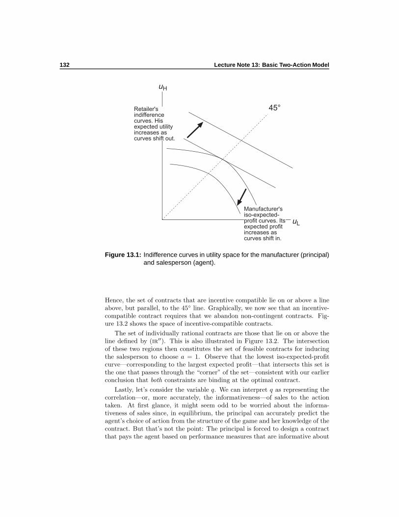
132 Lecture Note 13: Basic Two-Action Model
45°
uL
uH
Retailer's indifference curves. His expected utility increases as curves shift out.
Manufacturer's iso-expected-profit curves. Its expected profit increases as curves shift in.
Figure 13.1: Indifference curves in utility space for the manufacturer (principal)and salesperson (agent).
Hence, the set of contracts that are incentive compatible lie on or above a lineabove, but parallel, to the 45 line. Graphically, we now see that an incentive-compatible contract requires that we abandon non-contingent contracts. Fig-ure 13.2 shows the space of incentive-compatible contracts.
The set of individually rational contracts are those that lie on or above theline defined by (ir′′). This is also illustrated in Figure 13.2. The intersectionof these two regions then constitutes the set of feasible contracts for inducingthe salesperson to choose a = 1. Observe that the lowest iso-expected-profitcurve—corresponding to the largest expected profit—that intersects this set isthe one that passes through the “corner” of the set—consistent with our earlierconclusion that both constraints are binding at the optimal contract.
Lastly, let’s consider the variable q. We can interpret q as representing thecorrelation—or, more accurately, the informativeness—of sales to the actiontaken. At first glance, it might seem odd to be worried about the informa-tiveness of sales since, in equilibrium, the principal can accurately predict theagent’s choice of action from the structure of the game and her knowledge of thecontract. But that’s not the point: The principal is forced to design a contractthat pays the agent based on performance measures that are informative about

13.3 Two-outcome Model 133
Individually rational contracts
IC contracts
Both IR and IC contracts
45°
uL
uHIC
IRC/q
Optimalcontract
Figure 13.2: The set of feasible contracts.
the variable upon which she would truly like to contract, namely his action.The more informative these performance measures are—loosely, the more cor-related they are with action—the closer the principal is getting to the ideal ofcontracting on the agent’s action.
In light of this discussion it wouldn’t be surprising if the manufacturer’sexpected profit under the optimal contract for inducing a = 1 increases as qincreases. Clearly its expected revenue,
qxH + (1 − q)xL,
is increasing in q. Hence, it is sufficient to show merely that its expected cost,
qsH + (1 − q) sL,
is non-increasing in q. To do so, it is convenient to work in terms of utility(i.e., uH and uL) rather than directly with compensation. Let q1 and q2 be twodistinct values of q, with q1 < q2. Let
u1n
be the optimal contract (expressed
in utility terms) when q = q1.Define a = q1/q2 and define
uH = au1H + (1 − a)u1
L and
uL = u1L.
134 Lecture Note 13: Basic Two-Action Model
Let us now see that un satisfies both the ir and ic constraints when q = q2.Observe first that
q2uH + (1 − q2) uL = aq2u1H +
((1 − a)q2 + 1 − q2
)u1L
= q1u1H + (1 − q1)u
1L .
Given thatu1n
satisfies ir and ic when q = q1, it follows, by transitivity, that
un solves ir and ic when q = q2. We need, now, simply show that
q2u−1 (uH) + (1 − q2)u
−1 (uL) ≤ q1u−1(u1H
)+ (1 − q1)u
−1(u1L
).
To do this, observe that
u−1 (uH) ≤ au−1(u1H
)+ (1 − a)u−1
(u1L
)and
u−1 (uL) ≤ u−1(u1L
),
by Jensen’s inequality (recall u−1 (·) is convex). Hence we have
q2u−1 (uH) + (1 − q2) u
−1 (uL) ≤ q2
(au−1
(u1H
)+ (1 − a)u−1
(u1L
) )
+ (1 − q2)u−1(u1L
)
= q1u−1(u1H
)+ (1 − q1)u
−1(u1L
).
In other words, the manufacturer’s expected cost is no greater when q = q2 aswhen q = q1—as was to be shown.
Summary: Although we’ve considered the simplest of agency models in thissection, there are, nevertheless, some general lessons that come from this. First,the optimal contract for inducing an action other than the action that the agentfinds least costly requires a contract that is fully contingent on the performancemeasure. This is a consequence of the action being unobservable to the principal,not the agent’s risk aversion. When, however, the agent is risk averse, then theprincipal’s expected cost of solving the hidden-action problem is greater than itwould be in the benchmark full-information case: Exposing the agent to risk isinefficient (relative to the first best) and the cost of this inefficiency is borne bythe principal. The size of this cost depends on how good an approximation theperformance measure is for the variable upon which the principal really desiresto contract, the agent’s action. The better an approximation (statistic) it is, thelower is the principal’s expected cost. If, as here, that shift also raises expectedrevenue, then a more accurate approximation means greater expected profits.It is also worth pointing out that one result, which might seem as though itshould be general, is not: Namely, the result that compensation is increasingwith performance (e.g., sH > sL). Although this is true when there are only twopossible realizations of the performance measure (as we’ve proved), this resultdoes not hold generally when there are more than two possible realizations.
13.4 Multiple-outcomes Model 135
Multiple-outcomes Model 13.4Now we assume that there are multiple possible outcomes, including, possibly,an infinite number. Without loss of generality, we may assume the set of possiblesales levels is (0,∞), given that impossible levels in this range can be assignedzero probability. We will also assume, henceforth, that u (·) exhibits strict riskaversion (i.e., is strictly concave).
Recall that our problem is to solve program (13.3), on page 127. In thiscontext, we can rewrite the problem as
maxS(·)
∫ ∞
0
(x− S (x)) dF1 (x)
subject to
∫ ∞
0
u [S (x)] dF1 (x) − C ≥ UR and (13.7)
∫ ∞
0
u [S (x)] dF1 (x) − C ≥∫ ∞
0
u [S (x)] dF0 (x) , (13.8)
which are the ir and ic constraints, respectively. In what follows, we assumethat there is a well-defined density function, fa (·), associated with Fa (·) forboth a. For instance, if Fa (·) is differentiable everywhere, then fa (·) = F ′
a (·)and the
∫dFa (x) notation could be replaced with
∫fa (x) dx. Alternatively,
the possible outcomes could be discrete, x = x1, . . . , xN , in which case
fa (x) = Fa (x) − limx↑x
Fa (x)
and the∫dFa (x) notation could be replaced with
∑Nn=1 fa (xn).
We solve the above program using standard Kuhn-Tucker techniques. Letµ be the (non-negative) Lagrange multiplier on the incentive constraint andlet λ be the (non-negative) Lagrange multiplier on the individual rationalityconstraint. The Lagrangian of the problem is, thus,
L(S(·), λ, µ) =
∫ +∞
0
[x− S(x)] dF1(x) + λ
(∫ +∞
0
u(S(x))dF1(x) − C
)
+ µ
(∫ +∞
0
u(S(x))dF1(x) −∫ +∞
0
u(S(x))dF0(x) − C
).
The necessary first-order conditions are λ ≥ 0, µ ≥ 0, (13.7), (13.8),
u′ [S(x)]
(λ+ µ
[1 − f0(x)
f1(x)
])− 1 = 0, (13.9)
λ > 0 ⇒∫ +∞
0
u(S(x))dF1(x) = C + UR, and
136 Lecture Note 13: Basic Two-Action Model
µ > 0 ⇒∫ +∞
0
u(S(x))dF1(x) −∫ +∞
0
u(S(x))dF0(x) = C.
From our previous reasoning, we already know that the ic constraint isbinding. To see this again, observe that if it were not (i.e., µ = 0), then (13.9)would reduce to u′ [S (x)] = 1/λ for all x; that is, a fixed payment.11 But weknow a fixed-payment contract is not incentive compatible. It is also immediatethat the participation constraint must be satisfied as an equality; otherwise, themanufacturer could reduce the payment schedule, thereby increasing her profits,in a manner that preserved the incentive constraint (i.e., replace S∗ (x) withS (x), where S (x) = u−1 (u [S∗ (x)] − ε)).
Note that the necessary conditions above are also sufficient given the as-sumed concavity of u(·). At every point where it is maximized with respect tos, (
λ+ µ
[1 − f0(x)
f1(x)
])
must be positive—observe it equals
1
u′ (s)> 0
—so the second derivative with respect to s must, therefore, be negative.The least-cost contract inducing a = 1 therefore corresponds to a payment
schedule S(·) that varies with the level of sales in a non-trivial way given by(13.9). That expression might look complicated, but its interpretation is centralto the model and easy to follow. Observe, in particular, that because u′ (·)is a decreasing function (u (·), recall, is strictly concave), S (x) is positivelycorrelated with
λ+ µ
[1 − f0(x)
f1(x)
];
that is, the larger (smaller) is this term, the larger (smaller) is S (x).The reward for a given level of sales x depends upon the likelihood ratio
r(x) ≡ f0(x)
f1(x)
of the probability that sales are x when action a = 0 is taken relative to thatprobability when action a = 1 is taken.12 This ratio has a clear statisticalmeaning: It measures how more likely it is that the distribution from which saleshave been determined is F0(·) rather than F1(·). When r(x) is high, observingsales equal to x allows the manufacturer to draw a statistical inference that it
11Note that we’ve again established the result that, absent an incentive problem, a risk-neutral player should absorb all the risk when trading with a risk-averse player.
12Technically, if Fa (·) is differentiable (i.e., fa (·) is a probability density function), thenthe likelihood ratio can be interpreted as the probability that sales lie in (x, x + dx) whena = 0 divided by the probability of sales lying in that interval when a = 1.
13.4 Multiple-outcomes Model 137
is much more likely that the distribution of sales was actually F0(.); that is, thesalesperson did not expend effort promoting the product. In this case,
λ+ µ
[1 − f0(x)
f1(x)
]
is small (but necessarily positive) and S(x) must also be small as well. Whenr(x) is small, the manufacturer should feel rather confident that the salespersonexpended effort and it should, then, optimally reward him highly. That is,sales levels that are relatively more likely when the agent has behaved in thedesired manner result in larger payments to the agent than sales levels that arerelatively rare when the agent has behaved in the desired manner.
The minimum-cost incentive contract that induces the costly action a =1 in essence commits the principal (manufacturer) to behave like a Bayesianstatistician who holds some diffuse prior over which action the agent has taken:13
She should use the observation of sales to revise her beliefs about what actionthe agent took and she should reward the agent more for outcomes that causeher to revise upward her beliefs that he took the desired action and she shouldreward him less (punish him) for outcomes that cause a downward revision inher beliefs.14 As a consequence, the payment schedule is connected to sales onlythrough their statistical content (the relative differences in the densities), notthrough their accounting properties. In particular, there is now no reason tobelieve that higher sales (larger x) should be rewarded more than lower sales.
As an example of non-monotonic compensation, suppose that there are threepossible sales levels: low, medium, and high (xL, xM , and xH , respectively).Suppose, in addition, that
fa (x) =
13 , if x = xL2−a6 , if x = xM
2+a6 , if x = xH
.
Then
λ+ µ
[1 − f0(x)
f1(x)
]=
λ, if x = xL
λ− µ, if x = xM
λ+ µ3 , if x = xH
.
Hence, low sales are rewarded more than medium sales—low sales are unin-formative about the salesperson’s action, whereas medium sales suggest thatthe salesperson has not expended effort. Admittedly, non-monotonic compen-sation is rarely, if ever, observed in real life. We will see below what additionalproperties are required, in this model, to ensure monotonic compensation.
13A diffuse prior is one that assigns positive probability to each possible action.
14Of course, as a rational player of the game, the principal can infer that, if the contractis incentive compatible, the agent will have taken the desired action. Thus, there is not, insome sense, a real inference problem. Rather the issue is that, to be incentive compatible, theprincipal must commit to act as if there were an inference problem.
138 Lecture Note 13: Basic Two-Action Model
Note, somewhat implicit in our analysis to this point, is an assumption thatf1 (x) > 0 except, possibly, on a subset of x that are impossible (have zeromeasure). Without this assumption, (13.9) would entail division by zero, whichis, of course, not permitted. If, however, we let f1 (·) go to zero on some subsetof x that had positive measure under F0 (·), then we see that µ must also tendto zero because
λ+ µ
[1 − f0(x)
f1(x)
]
must be positive. In essence, then, the shadow price (cost) of the incentiveconstraint vanishes as f1 (·) goes to zero. This makes perfect sense: Were f1 (·)zero on some subset of x that could occur (had positive measure) under F0 (·),then the occurrence of any x in this subset, X0, would be proof that the agenthad failed to take the desired action. We can use this, then, to design a contractthat induces a = 1, but which costs the principal no more than the optimal full-information fixed-payment contract S (x) = sF1 . That is, the incentive problemceases to be costly; so, not surprisingly, its shadow cost is zero.
To see how we can construct such a contract when f1 (x) = 0 for all x ∈ X0,let
S (x) =
s+ ε, if x ∈ X0
sF1 , if x /∈ X0,
where ε > 0 is arbitrarily small (s, recall, is the greatest lower bound of thedomain of u (·)). Then
∫ +∞
0
u(S(x))dF1(x) = u(sF1)
and
∫ +∞
0
u(S(x))dF0(x) =
∫
X0
u (s+ ε) dF0 (x) +
∫
R+\X0
u(sF1)dF0 (x)
= u (s+ ε)F0 (X0) + u(sF1)(1 − F0 (X0)) .
From the last expression, it’s clear that∫ +∞0 u(S(x))dF0(x) → −∞ as ε → 0;
hence, the ic constraint is met trivially. By the definition of sF1 , ir is also met.That is, this contract implements a = 1 at full-information cost. Again, as wesaw in the two-outcome model, having a shifting support (i.e., the propertythat F0 (X0) > 0 = F1 (X0)) allows us to implement the desired action at full-information cost.
To conclude this section, we need to answer one final question. Does themanufacturer prefer to induce a = 1 or a = 0 given the “high” cost of theformer? The manufacturer’s choice can be viewed as follows: Either it imposesthe fixed-payment contract sF0 , which induces action a = 0, or it imposes thecontract S(·) that has been derived above, which induces action a = 1. Theexpected-profit-maximizing choice results from the simple comparison of thesetwo contracts; that is, the manufacturer imposes the incentive contract S(·) ifand only if:
E0 [x] − sF0 < E1 [x] − E1 [S(x)] (13.10)
13.5 Monotonicity of the Optimal Contract 139
The right-hand side of this inequality corresponds to the value of the maxi-mization program (13.3). Given that the incentive constraint is binding in thisprogram, this value is strictly smaller than the value of the same program with-out the incentive constraint; hence, just as we saw in the two-outcome case, thevalue is smaller than full-information profits, E1 [x] − sF1 . Observe, therefore,that it is possible that
E1 [x] − sF1 > E0 [x] − sF0 > E1 [x] − E1 [S(x)] :
Under full information the principal would induce a = 1, but not if there’s ahidden-action problem. In other words, imperfect observability of the agent’saction imposes a cost on the principal that may induce her to distort the actionthat she induces the agent to take.
Monotonicity of the OptimalContract 13.5
Let us suppose that (13.10) is, indeed, satisfied so that the contract S(·) de-rived above is the optimal contract. Can we exhibit additional and meaningfulassumptions that would imply interesting properties of the optimal contract?
We begin with monotonicity, the idea that greater sales should mean greatercompensation for the salesperson. As we saw above (page 137), there is noguarantee in the multiple-outcome model that this property should hold every-where. From (13.9), it does hold if and only if the likelihood ratio, r (x), is notdecreasing and increasing at least somewhere. As this is an important property,it has a name:
Definition 5 The likelihood ratio r (x) = f0 (x) /f1 (x) satisfies the monotonelikelihood ratio property(mlrp) if r (·) is non-increasing almost everywhere andstrictly decreasing on at least some set of x’s that occur with positive probabilitygiven action a = 1.
The mlrp states that the greater is the outcome (i.e., x), the greater the relativeprobability of x given a = 1 than given a = 0.15 In other words, under mlrp,better outcomes are more likely when the salesperson expends effort than whenhe doesn’t. To summarize:
Proposition 19 In the model of this section, if the likelihood ratio, r (·), satis-fies the monotone likelihood ratio property, then the salesperson’s compensation,S (·), under the optimal incentive contract for inducing him to expend effort(i.e., to choose a = 1) is non-decreasing everywhere.
15Technically, if fa (x) = F ′a (x), then we should say “the greater the relative probability of
an x ∈ (x, x + dx) given a = 1 than given a = 0.”
140 Lecture Note 13: Basic Two-Action Model
In fact, because we know that S (·) can’t be constant—a fixed-payment contractis not incentive compatible for inducing a = 1—we can conclude that S (·) must,therefore, be increasing over some set of x.16
Is mlrp a reasonable assumption? To some extent is simply a strengtheningof our assumption that E1 [x] > E0 [x], given it can readily be shown that mlrp
implies E1 [x] > E0 [x].17 Moreover, many standard distributions satisfy mlrp.But it quite easy to exhibit meaningful distributions that do not. For instance,consider our example above (page 137). We could model these distributions asthe consequence of a two-stage stochastic phenomenon: With probability 1/3,a second new product is successfully introduced that eliminates the demand forthe manufacturer’s product (i.e., xL = 0). With probability 2/3, this secondproduct is not successfully introduced and it is “business as usual,” with salesbeing more likely to be xM if the salesperson doesn’t expend effort and morelikely to be xH if he does. These “compound” distributions do not satisfy mlrp.In such a situation, mlrp is not acceptable and the optimal reward schedule isnot monotonic, as we saw.
Although there has been a lot of discussion in the literature on the mono-tonicity issue, it may be overemphasized. If we return to the economic realitythat the mathematics seeks to capture, the discussion relies on the assumptionthat a payment schedule with the feature that the salesperson is penalized forincreasing sales in some range does not actual induce a new agency problem.For instance, if the good is perishable or costly to ship, it might be possible forthe salesperson to pretend, when sales are xM , that they are xL (if the allegedly
16Even if mlrp does not hold, r (·) must be decreasing over some measurable range. To see
this, suppose it were not true; that is, suppose that r(·) is almost everywhere non-decreasingunder distribution F1(·). Note this entails that x and r(x) are non-negatively correlated underF1(·). To make the exposition easier, suppose for the purpose of this aside that fa(·) = F ′
a (·).Then
E1
»
f0(x)
f1(x)
–
=
Z ∞
0
„
f0(x)
f1(x)
«
f1(x)dx =
Z ∞
0f0(x)dx = 1
Because x and r(x) are non-negatively correlated, we thus have
Z ∞
0x[r(x) − E1r(x)]f1(x)dx ≥ 0.
Substituting, this implies
0 ≤Z ∞
0x[
f0(x)
f1(x)− 1]f1(x)dx =
Z ∞
0xf0(x)dx −
Z ∞
0xf1(x)dx = E0[x] − E1[x].
But this contradicts our assumption that investing (a = 1) yields greater expected revenuesthan does not investing (a = 0). Hence, by contradiction it must be that r(·) is decreasing oversome measurable range. But then this means that S(·) is increasing over some measurablerange. However, without mlrp, we can’t conclude that it’s not also decreasing over some othermeasurable range.
Conclusion: If E0[x] < E1[x], then S(·) is increasing over some set of x that has positive
probability of occurring given action a = 1 even if mlrp does not hold.
17This can most readily be seen from the previous footnote: Simply assume that r (·) satisfiesmlrp, which implies x and r (x) are negatively correlated. Then, following the remaining steps,it quickly falls out that E1 [x] > E0 [x].
13.6 Informativeness of the Performance Measure 141
unsold amount of the good cannot be returned). That is, a non-monotonicincentive scheme could introduce a new agency problem of making sure thesalesperson reports his sales honestly. Of course, if the manufacturer can verifythe salesperson’s inventory, a non-monotonic scheme might be possible. Butthink of another situation where the problem is to provide a worker (the agent)incentives to produces units of output; isn’t it natural, then, to think that theworker could very well stop his production at xL or destroy his extra produc-tion xM − xL? Think of yet another situation where the problem is to provideincentives to a manager; aren’t there many ways to spend money in a hardlydetectable way so as to make profits look smaller than what they actually are?In short, the point is that if the agent can freely and secretly diminish his per-formance, then it makes no sense for the principal to have a reward schedulethat is decreasing with performance over some range. In other words, there isoften an economic justification for monotonicity even when mlrp doesn’t hold.
Informativeness of thePerformance Measure 13.6
Now, we again explore the question of the informativeness of the performancemeasures used by the principal. To understand the issue, suppose that the man-ufacturer in our example can also observe the sales of another of its productssold by the salesperson. Let y denote these sales of the other good. These salesare, in part, also random, affected by forces outside the parties’ control; but also,possibly, determined by how much effort the salesperson expends promoting thefirst product. For example, consumers could consider the two goods comple-ments (or substitutes). Sales y will then co-vary positively (or negatively) withsales x. Alternatively, both goods could be normal goods, so that sales of ycould then convey information about general market conditions (the incomesof the customers). Of course, it could also be that the demand for the secondproduct is wholly unrelated to the demand for the first; in which case sales ywould be insensitive to the salesperson’s action.
Let f0(x, y) and f1(x, y) denote the joint probability densities of sales x andy for action a = 0 and a = 1. An incentive contract can now be a functionof both performance variables; that is, s = S(x, y). It is immediate that thesame approach as before carries through and yields the following optimalitycondition:18
u′ [S(x, y)]
(λ+ µ
[1 − f0(x, y)
f1(x, y)
])− 1 = 0. (13.11)
When is it optimal to make compensation a function of y as well as of x?
18Although we use the same letters for the Lagrange multipliers, it should be clear thattheir values at the optimum are not related to their values in the previous, one-performance-measure, contracting problem.
142 Lecture Note 13: Basic Two-Action Model
The answer is straightforward: When the likelihood ratio,
r(x, y) =f0(x, y)
f1(x, y),
actually depends upon y. Conversely, when the likelihood ratio is independentof y, then there is no gain from contracting on y to induce a = 1; indeed, itwould be sub-optimal in this case because such a compensation scheme wouldfail to satisfy (13.11). The likelihood ratio is independent of y if and only if thefollowing holds: There exist three functions h(·, ·), g0(·), and g1(·) such that, forall (x, y),
fa(x, y) = h(x, y)ga(x). (13.12)
Sufficiency is obvious (divide f0 (x, y) by f1 (x, y) and observe the ratio,g0(x)/g1(x), is independent of y). Necessity is also straightforward: Set h(x, y) =f1(x, y), g1(x) = 1, and g0(x) = r(x). This condition of multiplicative separa-bility, (13.12), has a well-established meaning in statistics: If (13.12) holds, thenx is a sufficient statistic for the action a given data (x, y). In words, were wetrying to infer a, our inference would be just as good if we observed only x asit would be if we observed the pair (x, y). That is, conditional on knowing x, yis uninformative about a.
This conclusion is, therefore, quite intuitive, once we recall that the valueof performance measures to our contracting property rests solely on their sta-tistical properties. The optimal contract should be based on all performancemeasures that convey information about the agent’s decision; but it is not de-sirable to include performance measures that are statistically redundant withother measures. As a corollary, there is no gain from considering ex post randomcontracts (e.g., a contract that based rewards on x+η, where η is some randomvariable—noise—distributed independently of a that is added to x).19 As asecond corollary, if the principal could freely eliminate noise in the performancemeasure—that is, switch from observing x + η to observing x—she would dobetter (at least weakly).
Conclusions from theTwo-action Model 13.7
It may be worth summing up all the conclusions we have reached within thetwo-action model in a proposition:
Proposition 20 If the agent is strictly risk averse, there is no shifting support,and the principal seeks to implement the costly action (i.e., a = 1), then theprincipal’s expected profits are smaller than under full (perfect) information.In some instances, this reduction in expected profits may lead the principal toimplement the “free” action (i.e., a = 0).
19Ex ante random contracts may, however, be of some value, as explained later.

13.7 Conclusions from the Two-action Model 143
• When (13.10) holds, the reward schedule imposes some risk on the risk-averse agent: Performances that are more likely when the agent takes thecorrect action a = 1 are rewarded more than performances that are morelikely under a = 0.
• Under mlrp (or when the agent can destroy output), the optimal rewardschedule is non-decreasing in performance.
• The optimal reward schedule depends only upon performance measures thatare sufficient statistics for the agent’s action.
To conclude, allow me to stress the two major themes that I would likethe reader to remember from this section. First, imperfect information impliesthat the contractual reward designed by the principal should perform two tasks:Share the risks involved in the relationship and provide incentives to induce theagent to undertake the desired action. Except in trivial cases (e.g., a risk-neutralagent or a shifting support), these two goals are in conflict. Consequently,the optimal contract may induce an inefficient action and a Pareto suboptimalsharing of risk.20 Second, the optimal reward schedule establishes a link betweenrewards and performances that depends upon the statistical properties of theperformance measures with respect to the agent’s action.
Bibliographic Notes
The analysis presented so far is fairly standard. The two-step approach—firstdetermine, separately, the optimal contracts for implementing a = 0 and a = 1,then choose which yields greater profits—is due to Grossman and Hart (1983).The analysis, in the two-outcome case, when q varies is also based on theirwork. They also consider the monotonicity of the optimal contract, althoughour analysis here draws more from Holmstrom (1979). Holmstrom is also thesource for the sufficient-statistic result. Finally, the expression
1
u′ [S (x)]= λ+ µ
[1 − f0(x)
f1(x)
],
which played such an important part in our analysis, is frequently referred toas the modified Borch sharing rule, in honor of Borch (1968), who worked outthe rules for optimal risk sharing absent a moral-hazard problem (hence, theadjective “modified”).
20Think of this as yet another example of the two-instruments principle.

144 Lecture Note 13: Basic Two-Action Model
General Framework 14As we’ve just seen, the two-action model yields strong results. But the modelincorporates a lot of structure and it relies on strong assumptions. Consequently,it’s hard to understand which findings are robust and which are merely artifactsof an overly simple formalization. The basic ideas behind the incentive modelare quite deep and it is worthwhile, therefore, to consider whether and how theygeneralize in less constrained situations.
Our approach is to propose a very general framework that captures thesituation described in the opening section. Such generality comes at the cost oftractability, so we will again find ourselves making specific assumptions. Butdoing so, we will try to motivate the assumptions we have to make and discusstheir relevance or underline how strong they are.
The situation of incentive contracting under hidden action or imperfect mon-itoring involves:
• a principal;
• an agent;
• a set of possible actions, A, from which the agent chooses (we take A tobe exogenously determined here);
• a set of verifiable signals or performance measures, X ;
• a set of benefits, B, for the principal that are affected by the agent’s action(possibly stochastically);
• rules (functions, distributions, or some combination) that relate elementsof A, X , and B;
• preferences for the principal and agent; and
• a bargaining game that establishes the contract between principal andagent (here, recall, we’ve fixed the bargaining game as the principal makesa take-it-or-leave-it offer, so that the only element of the bargaining gameof interest here is the agent’s reservation utility, UR).1
1We could also worry about whether the principal wants to participate—even make a take-it-or-leave-it offer—but because our focus is on the contract design and its execution, stagesof the game not reached if she doesn’t wish to participate, we will not explicitly consider thisissue here.
145
146 Lecture Note 14: General Framework
In many settings, including the one explored above, the principal’s benefit isthe same as the verifiable performance measure (i.e., b = x). But this need notbe the case. We could, for instance, imagine that there is a function mappingthe elements of A onto B. For example, the agent’s action could be fixingthe “true” quality of a product produced for the principal. This quality is also,then, the principal’s benefit (i.e., b = a). The only verifiable measure of quality,however, is some noisy (i.e., stochastic) measure of true quality (e.g., x = a+η,where η is some randomly determined distortion). As yet another possibility,the benchmark case of full information entails X = X ′ × A, where X ′ is someset of performance measures other than the action.
We need to impose some structure on X and B and their relationship to A:We take X to be a Euclidean vector space and we let dF (·|a) denote the prob-ability measure over X conditional on a. Similarly, we take B to be a Euclideanvector space and we let dG (·, ·|a) denote the joint probability measure over Band X conditional on a (when b ≡ x, we will write dF (·|a) instead of dG (·, ·|a)).This structure is rich enough to encompass the possibilities enumerated in theprevious paragraph (and more).
Although we could capture the preferences of the principal and agent withoutassuming the validity of the expected-utility approach to decision-making underuncertainty (we could, for instance, take as primitives the indifference curvesshown in Figures 13.1 and 13.2), this approach has not been taken in the lit-erature.2 Instead, the expected-utility approach is assumed to be valid and welet W (s, x, b) and U(s, x, a) denote the respective von Neumann-Morgensternutilities of the principal and of the agent, where s denotes the transfer from theprincipal to the agent (to principal from agent if s < 0).
In this situation, the obvious contract is a function that maps X into R. Wedefine such a contract as
Definition 6 A simple incentive contract is a reward schedule S : X → R thatdetermines the level of reward s = S(x) to be decided as a function of the realizedperformance level x.
There is admittedly no other verifiable variable that can be used to writemore elaborate contracts. There is, however, the possibility of creating verifiablevariables, by having one or the other or both players take verifiable actions fromsome specified action spaces. Consistent with the mechanism-design approach,the most natural interpretation of these new variables are that they are publicannouncements made by the players; but nothing that follows requires thisinterpretation. For example, suppose both parties have to report to the thirdparty charged with enforcing the contract their observation of x, or the agent
2Given some well-documented deficiencies in expected-utility theory (see, e.g., Epstein,1992; Rabin, 1997), this might, at first, seem somewhat surprising. However, as Epstein, §2.5,notes many of the predictions of expected-utility theory are robust to relaxing some of themore stringent assumptions that support it (e.g., such as the independence axiom). Given thetractability of the expected-utility theory combined with the general empirical support for thepredictions of agency theory, the gain from sticking with expected-utility theory would seemto outweigh the losses, if any, associated with that theory.
147
must report which action he has chosen. We could even let the principal makea “good faith” report of what action she believes the agent took, althoughthis creates its own moral-hazard problem because, in most circumstances, theprincipal could gain ex post by claiming she believes the agent’s action wasunacceptable. It turns out, as we will show momentarily, that there is nothingto be gained by considering such elaborate contracts; that is, there is no suchcontract that can improve over the optimal simple contract.
To see this, let us suppose that a contract determines a normal-form game tobe played by both players after the agent has taken his action.3,4 In particular,suppose the agent takes an action h ∈ H after choosing his action, but prior tothe realization of x; that he takes an actionm ∈ M after the realization of x; andthat the principal also takes an action n ∈ N after x has been realized. One ormore of these sets could, but need not, contain a single element, a “null” action.We assume that the actions in these sets are costless—if we show that costlesselaboration does no better than simple contracts, then costly elaboration alsocannot do better than simple contracts. Finally, let the agent’s compensationunder this elaborate contract be: s = S(x, h,m, n). We can now establish thefollowing:
Proposition 21 (Simple contracts are sufficient) For any general contract⟨H,M,N , S (·)
⟩and associated (perfect Bayesian) equilibrium, there exists a
simple contract S(·) that yields the same equilibrium outcome.
Proof: Consider a (perfect Bayesian) equilibrium of the original contract, in-volving strategies (a∗, h∗ (·) ,m∗(·, ·)) for the agent, where h∗ (a) and m∗ (a, x)describe the agent’s choice within H and M after he’s taken action a and per-formance x has been observed. Similarly, n∗(x) gives the principal’s choice ofaction as a function of the observed performance. Let us now consider the simplecontract defined as follows: For all x ∈ X ,
S(x) ≡ S(x, h∗ (a∗) ,m∗(x, a∗), n∗(x)).
Suppose that, facing this contract, the agent chooses an action a different froma∗. This implies that:
∫
XU(S(x), x, a)dF (x|a) >
∫
XU(S(x), x, a∗)dF (x|a∗),
3Note this may require that there be some way that the parties can verify that the agenthas taken an action. This may simply be the passage of time: The agent must take his actionbefore a certain date. Alternatively, there could be a verifiable signal that the agent has acted(but which does not reveal how he’s acted).
4Considering a extensive-form game with the various steps just considered would not alterthe reasoning that follows; so, we avoid these unnecessary details by restricting attention toa normal-form game.

148 Lecture Note 14: General Framework
or, using the definition of S(·),∫
XU[S(x, h∗ (a∗) ,m∗(x, a∗), n∗(x)), x, a
]dF (x|a) >
∫
XU[S(x, h∗ (a∗) ,m∗(x, a∗), n∗(x)), x, a∗
]dF (x|a∗).
Because, in the equilibrium of the normal-form game that commences after theagent chooses his action, h∗ (·) and m∗(·, ·) must satisfy the following inequality:
∫
XU[S(x, h∗ (a) ,m∗(x, a), n∗(x)), x, a
]dF (x|a) ≥
∫
XU[S(x, h∗ (a∗) ,m∗(x, a∗), n∗(x)), x, a
]dF (x|a),
it follows that∫
XU[S(x, h∗ (a) ,m∗(x, a), n∗(x)), x, a
]dF (x|a) >
∫
XU[S(x, h∗ (a∗) ,m∗(x, a∗), n∗(x)), x, a∗
]dF (x|a∗).
This contradicts the fact the a∗ is an equilibrium action in the game definedby the original contract. Hence, the simple contract S(·) gives rise to the sameaction choice, and therefore the same distribution of outcomes than the morecomplicated contract.
As a consequence, there is no need to consider sophisticated announcementmechanisms in this setting, at least in the simple situation we have described.The style in which we proved Proposition 21 should be familiar. In particular, itwas how we proved the Revelation Principle (Proposition 11 and Theorem 16).
The contracting problem under imperfect information can now easily bestated. The principal, having the bargaining power in the negotiation process,simply has to choose a (simple) contract, S(·), so as to maximize her expectedutility from the relationship given two constraints. First, the contract S(·)induces the agent to choose an action that maximizes his expected utility (i.e.,the ic constraint must be met). Second, given the contract and the action itwill induce, the agent must receive an expected utility at least as great as hisreservation utility (i.e., the ir constraint must be met). In this general setting,the ic constraint can be stated as the action induced, a, must satisfy
a ∈ argmaxa′
∫
XU(S(x), x, a′)dF (x|a′). (14.1)
Observe that choosing S(·) amounts to choosing a as well, at least when thereexists a unique optimal choice for the agent. To take care of the possibility ofmultiple optima for the agent, one can simply imagine that the principal chooses

149
a pair (S(·), a) subject to the incentive constraint (14.1). The ir constraint takesthe simple form:
maxa′
∫
XU(S(x), x, a′)dF (x|a′) ≥ UR. (14.2)
The principal’s problem is, thus,
max(S(·),a)
∫
XW (S(x), x, b)dG(b, x|a) (14.3)
s.t. (14.1) and (14.2).
Observe, as we did in Lecture Note 13, it is perfectly permissible to solve thismaximization program in two steps. First, for each action a, find the expected-profit-maximizing contract that implements action a subject to the ic and ir
constraints; this amounts to solving a similar program, taking action a as fixed:
maxS(.)
∫
XW (S(x), x, b)dG(b, x|a) (14.4)
s.t. (14.1) and (14.2).
Second, optimize the principal’s objectives with respect to the action to imple-ment; if we let Sa(·) denote the expected-profit-maximizing contract for imple-menting a, this second step consists of:
maxa∈A
∫
XW (Sa(x), x, b)dG(b, x|a).
In this more general framework, it’s worth revisiting the full-informationbenchmark. Before doing that, however, it is worth assuming that the domainof U (·, x, a) is sufficiently broad:
• Existence of a punishment: There exists some sP in the domain ofU (·, x, a) such that, for all a ∈ A,
∫
XU(sP , x, a)dF (x|a) < UR .
• Existence of a sufficient reward: There exists some sR in the do-main of U (·, x, a) such that, for all a ∈ A,
∫
XU(sR, x, a)dF (x|a) ≥ UR .
In light of the second assumption, we can always satisfy (14.2) for any action a(there is no guarantee, however, that we can also satisfy (14.1)).
With these two assumptions in hand, suppose that we’re in the full-infor-mation case; that is, X = X ′ ×A (note X ′ could be a single-element space, so
150 Lecture Note 14: General Framework
that we’re also allowing for the possibility that, effectively, the only performancemeasure is the action itself). In the full-information case, the principal can relyon forcing contracts ; that is, contracts that effectively leave the agent with nochoice over the action he chooses. Hence, writing (x′, a) for an element of X , aforcing contract for implementing a is
S(x′, a) = sP if a 6= a
= SF (x′) if a = a,
where SF (·) satisfies (14.2). Given that SF (x′) = sR satisfies (14.2) by as-sumption, we know that we can find an SF (·) function that satisfies (14.2).In equilibrium, the agent will choose to sign the contract—the ir constraint ismet—and he will take action a since this is his only possibility for getting atleast his reservation utility. Forcing contracts are very powerful because theytransform the contracting problem into a simple ex ante Pareto computationprogram:
max(S(·),a)
∫
XW (S(x), x, b)dG(b, x|a) (14.5)
s.t. (14.2),
where only the agent’s participation constraint matters. This ex ante Paretoprogram determines the efficient risk-sharing arrangement for the full-infor-mation optimal action, as well as the full-information optimal action itself. Itssolution characterizes the optimal contract under perfect information.
At this point, we’ve gone about as far as we can go without imposing morestructure on the problem. The next couple of Lecture Notes consider morestructured variations of the problem.

The Finite Model 15In this Lecture Note, we will assume A, the set of possible actions, is finite withJ elements. Likewise, the set of possible verifiable performance measures, X , isalso taken to be finite with N elements, indexed by n (although, at the end ofthis section, we’ll discuss the case where X = R). Given the world is, in reality,finite, this is the most general version of the principal-agent model (althoughnot necessarily the most analytically tractable).1
We will assume that the agent’s utility is additively separable between pay-ments and action. Moreover, it is not, directly, dependent on performance.Hence,
U (s, x, a) = u (s) − c(a);
where u : S → R maps some subset S of R into R and c : A → R maps theaction space into R. As before, we assume that S = (s,∞), where u (s) → −∞as s ↓ s. Observe that this assumption entails the existence of a punishment,sP , as described in the previous section. We further assume that u (·) is strictlymonotonic and concave (at least weakly). Typically, we will assume that u (·)is, in fact, strictly concave, implying the agent is risk averse. Note, that themonotonicity of u (·) implies that the inverse function u−1 (·) exists and, sinceu (S) = R, is defined for all u ∈ R.
We assume, now, that B ⊂ R and that the principal’s utility is a functiononly of the difference between her benefit, b, and her payment to the agent; thatis,
W (s, x, b) = w (b − s) ,
where w (·) is assumed to be strictly increasing and concave. In fact, in mostapplications—particularly most applications of interest in the study of strategyand organization—it is reasonable to assume that the principal is risk neutral.We will maintain that assumption here (the reader interested in the case of arisk-averse principal should consult Holmstrom, 1979, among other work). Inwhat follows, let B (a) = E b|a.
In addition to being discrete, we assume that there exists some partial orderon X (i.e., to give meaning to the idea of “better” or “worse” performance) and
1Limitations on measurement—of both inputs and outputs—make the world discrete. Forinstance, effort, measured as time on the job, can take only discrete values because onlydiscrete intervals of time can be measured. Similarly, output, measured as volume, can takeonly discrete values because only discrete intervals of volume can be measured. Because theworld is also bounded—each of us is allotted only so much time and there are only so manyatoms in the universe (under current cosmological theories)—it follows that the world is finite.
151
152 Lecture Note 15: The Finite Model
that, with respect to this partial order, X is a chain (i.e., if is the partialorder on X , then x x′ or x′ x for any two elements, x and x′ in X ). Becauseidentical signals are irrelevant, we may also suppose that no two elements of Xare the same (i.e., x ≺ x′ or x′ ≺ x for any two elements in X ). The mostnatural interpretation is that X is a subset of distinct real numbers—different“performance scores”—with ≤ as the partial order. Given these assumptions,we can write X = x1, . . . , xN, where xm ≺ xn if m < n. Likewise thedistribution function F (x|a) gives, for each x, the probability that an x′ xis realized conditional on action a. The corresponding density function is thendefined by
f (xn|a) =
F (x1|a) if n = 1F (xn|a) − F (xn−1|a) if n > 1
.
In much of what follows, it will be convenient to write fn (a) for f (xn|a). Itwill also be convenient to write the density as a vector:
f (a) = (f1 (a) , . . . , fN (a)) .
The “Two-step” Approach 15.1As we have done already in Lecture Note 13, we will pursue a two-step approachto solving the principal-agent problem:
Step 1: For each a ∈ A, the principal determines whether it can be imple-mented. Let AI denote the set of implementable actions. For each a ∈ AI ,the principal determines the least-cost contract for implementing a sub-ject to the ic and ir constraints. Let C (a) denote the principal’s expectedcost (expected payment) of implementing a under this least-cost contract.
Step 2: The principal then determines the solution to the maximization prob-lem
maxa∈AI
B (a) − C (a) .
If a∗ is the solution to this maximization problem, the principal offers theleast-cost contract for implementing a∗.
Note that this two-step process is analogous to a standard production prob-lem, in which a firm, first, solves its cost-minimization problems to determinethe least-cost way of producing any given amount of output (i.e., derives itscost function); and, then, it produces the amount of output that maximizes thedifference between revenues (benefits) and cost. As with production problems,the first step is generally the harder step.
The full-information benchmark
As before, we consider as a benchmark the case where the principal can observeand verify the agent’s action. Consequently, as we discussed at the end of
15.1 The “Two-step” Approach 153
Lecture Note 14, the principal can implement any action a that she wants usinga forcing contract: The contract punishes the agent sufficiently for choosingactions a 6= a that he would never choose any action other than a; and thecontract rewards the agent sufficiently for choosing a that he is just willing tosign the principal’s contract. This last condition can be stated formally as
u (s) − c (a) = UR, (irF )
where s is what the agent is paid if he chooses action a. Solving this lastexpression for s yields
s = u−1 [UR + c (a)] ≡ CF (a) .
The function CF (·) gives the cost, under full information, of implementingactions.
The hidden-action problem
Now, and henceforth, we assume that a hidden-action problem exists. Conse-quently, the only feasible contracts are those that make the agent’s compensationcontingent on the verifiable performance measure. Let s (x) denote the paymentmade to the agent under such a contract if x is realized. It will prove convenientto write sn for s (xn) and to consider the compensation vector s = (s1, . . . , sN).The optimal—expected-cost-minimizing—contract for implementing a (assum-ing it can be implemented) is the contract that solves the following program:2
mins
f (a) · s
subject toN∑
n=1
fn (a)u (sn) − c (a) ≥ UR
(the ir constraint) and
a ∈ maxa
N∑
n=1
fn (a)u (sn) − c (a)
(the ic constraint—see (14.1)). Observe that an equivalent statement of the ic
constraint is
N∑
n=1
fn (a)u (sn) − c (a) ≥N∑
n=1
fn (a)u (sn) − c (a) ∀a ∈ A.
As we’ve seen above, it is often easier to work in terms of utility paymentsthan in terms of monetary payments. Specifically, because u (·) is invertible,
2Observe, given the separability between the principal’s benefit and cost, minimizing herexpected wage payment is equivalent to maximizing her expected profit.

154 Lecture Note 15: The Finite Model
we can express a contract as an N -dimensional vector of contingent utilities,u = (u1, . . . , uN ), where un = u (sn). Using this “trick,” the principal’s programbecomes
minu
N∑
n=1
fn (a)u−1 (un) (15.1)
subject tof (a) · u− c (a) ≥ UR (ir)
andf (a) · u − c (a) ≥ f (a) · u− c (a) ∀a ∈ A. (ic)
Definition 7 An action a is implementable if there exists at least one contractsolving ( ir) and ( ic).
A key result is the following:
Proposition 22 If a is implementable, then there exists a contract that imple-ments a and satisfies ( ir) as an equality. Moreover, ( ir) is met as an equality(i.e., is binding) under the optimal contract for implementing a.
Proof: Suppose not: Let u be a contract that implements a and suppose that
f (a) · u − c (a) > UR.
Defineε = f (a) · u− c (a) − UR.
By assumption, ε > 0. Consider a new contract, u, where un = un − ε. Byconstruction, this new contract satisfies (ir). Moreover, because
f (a) · u = f (a) · u − ε,
for all a ∈ A, this new contract also satisfies (ic). Observe, too, that this newcontract is superior to u: It satisfies the contracts, while costing the principalless. Hence, a contract cannot be optimal unless (ir) is an equality under it.
In light of this proposition, it follows that an action a can be implementedif there is a contract u that solves the following system:
f (a) · u − c (a) = UR (15.2)
and
f (a) · u − c (a) ≤ UR ∀a ∈ A\ a (15.3)
(where (15.3) follows from (ic) and (15.2)). We are now in position to establishthe following proposition:
15.1 The “Two-step” Approach 155
Proposition 23 Action a is implementable if and only if there is no strategyfor the agent that induces the same density over signals as a and which coststhe agent less, in terms of expected disutility, than a (where “strategy” refers tomixed, as well as, pure strategies).
Proof: Let j = 1, . . . , J − 1 index the elements in A other than a. Then thesystem (15.2) and (15.3) can be written as J + 1 inequalities:
f (a) · u ≤ UR + c (a)[−f (a)] · u ≤ −UR − c (a)f (a1) · u ≤ UR + c (a1)
...f (aJ−1) · u ≤ UR + c (aJ−1)
By a well-known result in convex analysis (see, e.g., Rockafellar, 1970, page 198),there is a u that solves this system if and only if there is no vector
µ = (µ+, µ−, µ1, . . . , µJ−1) ≥ 0J+1
(where 0K is a K-dimensional vector of zeros) such that
µ+f (a) + µ− [−f (a)] +
J−1∑
j=1
µjf (aj) = 0N (15.4)
and
µ+ [UR + c (a)] + µ− [−UR − c (a)] +J−1∑
j=1
µj [UR + c (aj)] < 0. (15.5)
Observe that if such a µ exists, then (15.5) entails that not all elements can bezero. Define µ∗ = µ+−µ−. By post-multiplying (15.4) by 1N (anN -dimensionalvector of ones), we see that
µ∗ +
J−1∑
j=1
µj = 0. (15.6)
Equation (15.6) implies that µ∗ < 0. Define σj = µj/ (−µ∗). By constructioneach σj ≥ 0 (with at least some being strictly greater than 0) and, from (15.6),∑J−1j=1 σj = 1. Hence, we can interpret these σj as probabilities and, thus, as a
mixed strategy over the elements of A\ a. Finally, observe that if we divideboth sides of (15.4) and (15.5) by −µ∗ and rearrange, we can see that (15.4)and (15.5) are equivalent to
f (a) =J−1∑
j=1
σjf (aj) (15.7)
156 Lecture Note 15: The Finite Model
and
c (a) >J−1∑
j=1
σjc (aj) ; (15.8)
that is, there is a contract u that solves the above system of inequalities ifand only if there is no (mixed) strategy that induces the same density over theperformance measures as a (i.e., (15.7)) and that has lower expected cost (i.e.,(15.8)).
The truth of the necessity condition (only if part) of Proposition 23 isstraightforward: Were there such a strategy—one that always produced thesame expected utility over money as a, but which cost the agent less than a—then it would clearly be impossible to implement a as a pure strategy. Whatis less obvious is the sufficiency (if part) of the proposition. Intuitively, if thedensity over the performance measure induced by a is distinct from the densityinduced by any other strategy, then the performance measure is informativewith respect to determining whether a was the agent’s strategy or whether heplayed a different strategy. Because the range of u (·) is unbounded, even asmall amount of information can be exploited to implement a by rewarding theagent for performance that is relatively more likely to occur when he plays thestrategy a, or by punishing him for performance that is relatively unlikely tooccur when he plays the strategy a, or both .3 Of course, even if there are otherstrategies that induce the same density as a, a is still implementable if the agentfinds these other strategies more costly than a.
Before solving the principal’s problem (Step 1, page 152), it’s worth con-sidering, and then dismissing, two “pathological” cases. The first is the abilityto implement least-cost actions at their full-information cost. The second isthe ability to implement any action at its full-information cost when there is ashifting support (of the right kind).
Definition 8 An action a is a least-cost action if a ∈ argmina∈A c (a). Thatis, a is a least-cost action if the agent’s disutility from choosing any other actionis at least as great as his disutility from choosing a.
Proposition 24 If a is a least-cost action, then it is implementable at its full-information cost.
3We can formalize this notion of informationally distinct as follows: The condition that
no strategy duplicate the density over performance measures induced by a is equivalent tosaying that there is no density (strategy) (σ1, . . . , σJ−1) over the other J − 1 elements of Asuch that
f(a) =
J−1X
j=1
σj f(aj).
Mathematically, that’s equivalent to saying that f(a) is not a convex combination off(a)a∈A\a; or, equivalently that f(a) is not in the convex hull of f(a)|a 6= a. SeeHermalin and Katz (1991) for more on this “convex-hull” condition and its interpretation.Finally, from Proposition 23, the condition that f(a) not be in the convex hull of f(a)|a 6= ais sufficient for a to be implementable.

15.1 The “Two-step” Approach 157
Proof: Consider the fixed-payment contract that pays the agent un = UR +c (a) for all n. This contract clearly satisfies (ir) and, because c (a) ≤ c (a) forall a ∈ A, it also satisfies (ic). The cost of this contract to the principal isu−1 [UR + c (a)] = CF (a), the full-information cost.
Of course, there is nothing surprising to Proposition 24: When the principalwishes to implement a least-cost action, her interests and the agent’s are per-fectly aligned; that is, there is no agency problem. Consequently, it is notsurprising that the full-information outcome obtains.
Definition 9 There is a meaningful shifting support associated with action aif there exists a subset of X , X0, such that F (X0|a) > 0 = F (X0|a) for allactions a such that c (a) < c (a).
Proposition 25 Let there be a meaningful shifting support associated with ac-tion a. Then action a is implementable at its full-information cost.
Proof: Fix some arbitrarily small ε > 0 and define uP = u (s+ ε). Considerthe contract u that sets um = uP if xm ∈ X0 (where X0 is defined above) andthat sets un = UR + c (a) if xn /∈ X0. It follows that f (a) · u = UR + c (a); thatf (a) · u → −∞ as ε ↓ 0 for a such that c (a) < c (a); and that
f (a) · u − c (a) ≤ UR + c (a) − c (a) ≤ f (a) · u − c (a)
for a such that c (a) ≥ c (a). Consequently, this contract satisfies (ir) and (ic).Moreover, the equilibrium cost of this contract to the principal is u−1 [UR + c (a)],the full-information cost.
Intuitively, when there is a meaningful shifting support, observing an x ∈ X0
is proof that the agent took an action other than a. Because the principal hasthis proof, she can punish the agent as severely as she wishes when such an xappears (in particular, she doesn’t have to worry about how this punishmentchanges the risk faced by the agent, given the agent is never in jeopardy ofsuffering this punishment if he takes the desired action, a).4 Moreover, such adraconian punishment will deter the agent from taking an action that inducesa positive probability of suffering the punishment. In effect, such actions havebeen dropped from the original game, leaving a as a least-cost action of the new
4It is worth noting that this argument relies on being able to punish the agent sufficientlyin the case of an x ∈ X0. Whether the use of such punishments is really feasible could,in some contexts, rely on assumptions that are overly strong. First, that the agent hasn’t(or can contractually waive) protections against severe punishments. For example, in theEnglish common-law tradition, this is generally not true; moreover, courts in these countriesare generally loath to enforce contractual clauses that are deemed to be penalties. Second,that the agent has faith in his understanding of the distributions (i.e., he is sure that takingaction a guarantees that an x ∈ X0 won’t occur). Third, that the agent has faith in his ownrationality; that is, in particular, he is sufficiently confident that won’t make a mistake (i.e.,choose an a such that F (X0|a) > 0).
158 Lecture Note 15: The Finite Model
game. It follows, then, from Proposition 24, that a can be implemented at itsfull-information cost.
It is worth noting that the full-information benchmark is just a special caseof Proposition 25, in which the support of f (a) lies on a separate plane, X ′×a,for each action a.
Typically, it is assumed that the action the principal wishes to implementis neither a least-cost action, nor has a meaningful shifting support associatedwith it. Henceforth, we will assume that the action that principal wishes toimplement, a, is not a least-cost action (i.e., ∃a ∈ A such that c (a) < c (a)).Moreover, we will rule out all shifting supports by assuming that fn (a) > 0 forall n and all a.
We now consider the whether there is a solution to Step 1 when there is noshifting support and the action to be implemented is not a least-cost action.That is, we ask the question: If a is implementable is there an optimal contractfor implementing it? We divide the analysis into two cases: u (·) affine (riskneutral) and u (·) strictly concave (risk averse).
Proposition 26 Assume u (·) is affine and that a is implementable. Then a isimplementable at its full-information cost.
Proof: Let u solve (ir) and (ic). From Proposition 22, we may assume that(ir) is binding. Then, because u (·) and, thus, u−1 (·) are affine:
N∑
n=1
fn (a)u−1 (un) = u−1
(N∑
n=1
fn (a) un
)= u−1 [UR + c (a)] ,
where the last inequality follows from the fact that (ir) is binding.
Note, given that we can’t do better than implement an action at full-informationcost, this proposition also tells us that, with a risk-neutral agent, an optimalcontract exists for inducing any implementable action. The hidden-action prob-lem (the lack of full information) is potentially costly to the principal for tworeasons. First, it may mean a desired action is not implementable. Second, evenif it is implementable, it may be implementable at a higher cost. Proposition26 tells us that this second source of cost must be due solely to the agent’s riskaversion; an insight consistent with those derived earlier.
In fact, if we’re willing to assume that the principal’s benefit is alienable—that is, she can sell the rights to receive it to the agent—and that the agentis risk neutral, then we can implement the optimal full-information action, a∗
(i.e., the solution to Step 2 under full information) at full-information cost. Inother words, we can achieve the complete full-information solution in this case:
Proposition 27 (Selling the store) Assume that u (·) is affine and that theprincipal’s benefit is alienable. Then the principal can achieve the same expectedutility with a hidden-action problem as she could under full information.
15.1 The “Two-step” Approach 159
Proof: Under full information, the principal would induce a∗ where
a∗ ∈ argmaxa∈A
B (a) − CF (a) .
Definet∗ = B (a∗) − CF (a∗) .
Suppose the principal offers to sell the right to her benefit to the agent for t∗. Ifthe agent accepts, then the principal will enjoy the same utility she would haveenjoyed under full information. Will the agent accept? Note that because u (·)is affine, there is no loss of generality in assuming it is the identity function. Ifhe accepts, he faces the problem
maxa∈A
∫
B(b− t∗) dG (b|a) − c (a) .
This is equivalent to
maxa∈A
B (a) − c (a) − B (a∗) + c (a∗) + UR; or to
maxa∈A
B (a) − [c (a) + UR] −B (a∗) + c (a∗) + 2UR.
Because B (a)− [c (a) + UR] = B (a)−CF (a), rational play by the agent condi-tional on accepting means his utility will be UR; which also means he’ll accept.
People often dismiss the case where the agent is risk neutral by claiming thatthere is no agency problem because the principal could “sell the store (produc-tive asset)” to the agent. As this last proposition makes clear, such a conclusionrelies critically on the ability to literally sell the asset; that is, if the principal’sbenefit is not alienable, then this conclusion might not hold.5 In other words, itis not solely the agent’s risk aversion that causes problems with a hidden action.
Corollary 5 Assume that u (·) is affine and that the principal’s benefit equalsthe performance measure (i.e., B = X and G (·|a) = F (·|a)). Then the principalcan achieve the same expected utility with a hidden-action problem as she couldunder full information.
Proof: Left to the reader. (Hint: Let s (x) = x− t, where t is a constant.)
Now we turn our attention to the case where u (·) is strictly concave (theagent is risk averse). Observe (i) this entails that u−1 (·) is strictly convex; (ii),because S is an open interval, that u (·) is continuous; and (iii) that u−1 (·) iscontinuous.
5To see this, suppose the benefit is unalienable. Assume, too, that A = 1/4, 1/2, 3/4,X = 1, 2, c (a) =
√a, f2 (a) = a, UR = 0, and B (a) = 4−4
`
a − 12
´2. Then it is readily seen
that a∗ = 1/2. However, from Proposition 23, a∗ is not implementable, so the full-informationoutcome is unobtainable when the action is hidden (even though the agent is risk neutral).
160 Lecture Note 15: The Finite Model
Proposition 28 Assume that u (·) is strictly concave. If a is implementable,then there exists a unique contract that implements a at minimum expected cost.
Proof: Existence.6 Define
Ω (u) =
N∑
n=1
fn (a)u−1 (un) . (15.9)
The strict convexity and continuity of u−1 (·) implies that Ω (·) is also a strictlyconvex and continuous function. Observe that the principal’s problem is tochoose u to minimize Ω (u) subject to (ir) and (ic). Let U be the set of contractsthat satisfy (ir) and (ic) (by assumption, U is not empty). Were U closedand bounded, then a solution to the principal’s problem would certainly existbecause Ω (·) is a continuous real-valued function.7 Unfortunately, U is notbounded (although it is closed given that all the inequalities in (ir) and (ic) areweak inequalities). Fortunately, we can artificially bound U by showing that anysolution outside some bound is inferior to a solution inside the bound. Considerany contract u0 ∈ U and consider the contract u∗, where u∗n = UR + c (a). LetUIR be the set of contracts that satisfy (ir). Note that U ⊂ UIR. Note, too,that both U and UIR are convex sets. Because Ω (·) has a minimum on UIR,namely u∗, the set
V ≡u ∈ UIR|Ω (u) ≤ Ω
(u0)
is closed, bounded, and convex.8 By construction, U∩V is non-empty; moreover,for any u1 ∈ U ∩V and any u2 ∈ U\V , Ω
(u2)> Ω
(u1). Consequently, nothing
is lost be limiting the search for an optimal contract to U ∩ V . The set U ∩ Vis closed and bounded and Ω (·) is continuous, hence it follows that an optimalcontract must exist.
Uniqueness. Suppose the optimal contract, u, were not unique. That is,there exists another contract u such that Ω (u) = Ω (u) (where Ω (·) is definedby (15.9)). It is readily seen that if these two contracts each satisfy both the(ir) and (ic) constraints, then any convex combination of them must as well(i.e., both are elements of U , which is convex). That is, the contract
uλ ≡ λu + (1 − λ) u,
λ ∈ (0, 1) must be feasible (i.e., satisfy (ir) and (ic)). Because Ω (·) is strictlyconvex, Jensen’s inequality implies
Ω (uλ) < λΩ (u) + (1 − λ)Ω (u) = Ω (u) .
6The existence portion of this proof is somewhat involved mathematically and can beomitted without affecting later comprehension of the material.
7This is a well-known result from analysis (see, e.g., Fleming, 1977, page 49).
8The convexity of V follows because Ω (·) is a convex function and UIR is a convex set.That V is closed follows given UIR is also closed. To see that V is bounded, recognize that, asone “moves away” from u∗—while staying in UIR—Ω (u) increases. Because Ω (·) is convex,any such movement away from u∗ must eventually (i.e., for finite u) lead to a Ω (u) > Ω
`
u0´
(convex functions are unbounded above). Hence V is bounded.
15.2 Properties of the Optimal Contract 161
But this contradicts the optimality of u. By contradiction, uniqueness is estab-lished.
Having concluded that a solution to Step 1 exists, we can—at last—calculatewhat it is. From Proposition 26, the problem is trivial if u (·) is affine, so we willconsider only the case in which u (·) is strictly concave. The principal’s problemis a standard nonlinear programming problem: Minimize a convex function(i.e.,
∑Nn=1 fn (a)u−1 (un)) subject to J constraints (one individual rationality
constraint and J−1 incentive compatibility constraints, one for each action otherthan a). If we further assume, as we do henceforth, that u (·) is differentiable,then the standard Lagrange-multiplier techniques can be employed. Specifically,let λ be the Lagrange multiplier on the ir constraint and let µj be the Lagrangemultiplier on the ic constraint between a and aj , where j = 1, . . . , J−1 indexesthe elements of A other than a. It is readily seen that the first-order conditionwith respect to the contract are
fn (a)
u′ [u−1 (un)]− λfn (a) −
J−1∑
j=1
µj [fn (a) − fn (aj)] = 0; n = 1, . . . , N .
We’ve already seen (Proposition 22) that the ir constraint binds, hence λ > 0.Because a is not a least-cost action and there is no shifting support, it is readilyshown that at least one ic constraint binds (i.e., ∃j such that µj > 0). It’sconvenient to rewrite the first-order condition as
1
u′ [u−1 (un)]= λ+
J−1∑
j=1
µj
(1 − fn (aj)
fn (a)
); n = 1, . . . , N . (15.10)
Note the resemblance between (15.10) and (13.9) in Section 13.4. The differenceis that, now, we have more than one Lagrange multiplier on the actions (aswe now have more than two actions). In particular, we can give a similarinterpretation to the likelihood ratios, fn (aj) /fn (a), that we had in that earliersection; with the caveat that we now must consider more than one action.
Properties of the OptimalContract 15.2
Having solved for the optimal contract, we can now examine its properties. Inparticular, we will consider three questions:
1. Under what conditions does the expected cost of implementing an actionunder the optimal contract for the hidden-action problem exceed the full-information cost of implementing that action?
2. Recall the performance measures, x, constitute distinct elements of achain. Under what conditions is the agent’s compensation increasing withthe value of the signal (i.e., when does x ≺ x′ imply s (x) ≤ s (x′))?
162 Lecture Note 15: The Finite Model
3. Consider two principal-agent models that are identical except that theinformation structure (i.e., f (a) |a ∈ A) in one is more informative thanthe information structure in the other. How do the costs of implementingactions vary between these two models.
The answer to the first question is given by
Proposition 29 Consider a hidden-information problem. Assume there is noshifting support (i.e., fn (a) > 0 for all n and all a). Assume, too, that u (·) isstrictly concave. If a is not a least-cost action, then it cannot be implementedat its full-information cost.
Proof: If a is not implementable, then the result is obvious; hence, we’ll assumea is implementable. Define UIR to be the set of all contracts that satisfy their constraint for a. Let u∗ be the contract in which u∗n = UR + c (a) for all n.Note u∗ ∈ UIR. Finally define,
Ω (u) =
N∑
n=1
fn (a)u−1 (un) .
Because u (·) is strictly concave, the principal’s expected cost if the agent choosesa under contract u, Ω (u), is a strictly convex function of u. By Jensen’s in-equality and the fact that there is no shifting support, Ω (·), therefore, has aunique minimum in UIR, namely u∗. Clearly, Ω (u∗) = CF (a). The result,then, follows if we can show that u∗ is not incentive compatible. Given that ais not a least-cost action, there exists an a such that c (a) > c (a). But
f (a) · u∗ − c (a) = UR + c (a) − c (a) > UR = f (a) · u∗ − c (a) ;
that is, u∗ is not incentive compatible.
Note the elements that go into this proposition if a is implementable: Theremust be an agency problem—mis-alignment of interests (i.e., a is not least cost);there must, in fact, be a significant hidden-action problem (i.e., no shiftingsupport); and the agent must be risk averse. We saw earlier that without any oneof these elements, an implementable action is implementable at full-informationcost (Propositions 24–26); that is, each element is individually necessary forcost to increase when we go from full information to a hidden action. This lastproposition shows, inter alia, that they are collectively sufficient for the cost toincrease.
Next we turn to the second question. We already know from our analysis ofthe two-action model that the assumptions we have so far made are insufficientfor us to conclude that compensation will be monotonic. From our analysisof that model, we might expect that we need some monotone likelihood ratioproperty. In particular, we assume
MLRP: Assume there is no shifting support. Then the monotone likelihoodratio property is said to hold if, for any a and a in A, c (a) ≤ c (a) implies thatfn (a) /fn (a) is nonincreasing in n.
15.2 Properties of the Optimal Contract 163
Intuitively, mlrp is the condition that actions that the agent finds more costlybe more likely to produce better performance.
Unlike the two-action case, however, mlrp is not sufficient for us to obtainmonotone compensation (see Grossman and Hart, 1983, for an example in whichmlrp is satisfied but compensation is non-monotone). We need an additionalassumption:
CDFP: The agency problem satisfies the concavity of distribution functionproperty if, for any a, a′, and a in A,
c (a) = λc (a) + (1 − λ) c (a′) ∃λ ∈ (0, 1)
implies that F (·|a) first-order stochastically dominates λF (·|a)+(1 − λ)F (·|a′).9
Another way to state the cdfp is that the distribution over performance isbetter—more likely to produce high signals—if the agent plays a pure strategythan it is if he plays any mixed strategy over two actions when that mixedstrategy has the same expected disutility as the pure strategy.
We can now answer the second question:
Proposition 30 Assume there is no shifting support, that u (·) is strictly con-cave and differentiable, and that mlrp and cdfp are met. Then the optimalcontract given the hidden-action problem satisfies s1 ≤ · · · ≤ sN .
Proof: Let a be the action the principal wishes to implement. If a is a least-cost action, then the result follows from Proposition 24; hence assume that ais not a least-cost action. Let A′ = a|c (a) ≤ c (a); that is, A′ is the setof actions that cause the agent less disutility than a. Consider the principal’sproblem of implementing a under the assumption that the space of contracts isA′. By mlrp, fn (a) /fn (a) is nonincreasing in n for all a ∈ A′, so it followsfrom (15.10) that s1 ≤ · · · ≤ sN under the optimal contract for this restrictedproblem. The result then follows if we can show that this contract remainsoptimal when we expand A′ to A—adding actions cannot reduce the cost ofimplementing a, hence we are done if we can show that the optimal contractfor the restricted problem is incentive compatible in the unrestricted problem.That is, if there is no a, c (a) > c (a), such that
f (a) · u − c (a) > f (a) · u − c (a) , (15.11)
where u = (u (s1) , . . . , u (sN )). As demonstrated in the proof of Proposition 29,the incentive compatibility constraint between a and at least one a′ ∈ A′,c (a′) < c (a), is binding; i.e.,
f (a′) · u − c (a′) = f (a) · u − c (a) . (15.12)
9Recall that distribution G (·) first-order stochastically dominates distribution H (·) ifG (z) ≤ H (z) for all z and strictly less than for some z.
164 Lecture Note 15: The Finite Model
Because c (a) ∈ (c (a′) , c (a)), there exists a λ ∈ (0, 1) such that c (a) = (1 − λ) c (a′)+λc (a). Using cdfp and the fact that u (s1) ≤ · · · ≤ u (sN ), we have
f (a) · u− c (a) ≥ (1 − λ) f (a′) · u + λf (a) · u − c (a)
= (1 − λ) [f (a′) · u− c (a′)] + λ [f (a) · u − c (a)] .
But this and (15.12) are inconsistent with (15.11); that is, (15.11) cannot hold,as was required.
Lastly, we come to question 3. An information structure for a principal-agent problem is F ≡ f (a) |a ∈ A. A principal-agent problem can, then, besummarized as P = 〈A,X ,F, B (·) , c (·) , u (·) , UR〉.
Proposition 31 Consider two principal-agent problems that are identical ex-cept for their information structures (i.e., consider
P1 =⟨A,X ,F1, B (·) , c (·) , u (·) , UR
⟩
andP2 =
⟨A,X ,F2, B (·) , c (·) , u (·) , UR
⟩).
Suppose there exists a stochastic transformation matrix Q (i.e., a garbling)10
such that f2 (a) = Qf1 (a) for all a ∈ A, where f i (a) denotes an element ofFi. Then, for all a ∈ A, the principal’s expected cost of optimally implementingaction a in the first principal-agent problem, P1, is not greater than her expectedcost of optimally implementing a in the second principal-agent problem, P2.
Proof: Fix a. If a is not implementable in P2, then the result follows im-mediately. Suppose, then, that a is implementable in P2 and let u2 be theoptimal contract for implementing a in that problem. Consider the contractu1 = Q⊤u2.11 We will show that u1 implements a in P1. Because
f1 (a)⊤
u1 = f1 (a)⊤
Q⊤u2 = f2 (a)⊤
u2,
the fact that u2 satisfies ir and ic in P2 can readily be shown to imply that u1
satisfies ir and ic in P1. The principal’s cost of optimally implementing a in P1
is no greater than her cost of implementing a in P1 using u1. By construction,u1n = q⊤
·nu2, where q·n is the nth column of Q. Because sin = u−1
(uin)
andu−1 (·) is convex, it follows from Jensen’s Inequality that
s1n ≤N∑
m=1
qmns2m
10A stochastic transformation matrix, sometimes referred to as a garbling, is a matrix inwhich each column is a probability density (i.e., has non-negative elements that sum to one).
11For this proof it is necessary to distinguish between row vectors and column vectors, aswell as transposes of matrices. All vectors should be assumed to be column vectors. To makea vector x a row vector, we write x⊤. Observe that H⊤, where H is a matrix, is the transposeof H. Observe that x⊤y is the dot-product of x and y (what we’ve been writing as x · y).

15.3 A Continuous Performance Measure 165
(recall q·n is a probability vector). Consequently,
N∑
n=1
f1n (a) s1n ≤
N∑
n=1
f1n (a)
N∑
m=1
qmns2m =
N∑
m=1
f2n (a) s2n.
The result follows.
Proposition 31 states that if two principal-agent problems are the same,except that they have different information structures, where the informationstructure of the first problem is more informative than the information structureof the second problem (in the sense of Blackwell’s Theorem), then the principal’sexpected cost of optimally implementing any action is no greater in the firstproblem than in the second problem. By strengthening the assumptions slightly,we can, in fact, conclude that the principal’s expected cost is strictly less in thefirst problem. In other words, making the signal more informative about theagent’s action makes the principal better off. This is consistent with our earlierfindings that (i) the value of the performance measures is solely their statisticalproperties as correlates of the agent’s action; and (ii) the better correlates—technically, the more informative—they are, the lower the cost of the hidden-action problem.
It is worth observing that Proposition 31 implies that the optimal incentivescheme never entails paying the agent with lotteries over money (i.e., randomlymapping the realized performance levels via weights Q into payments).
A Continuous PerformanceMeasure 15.3
Suppose that X were a real interval—which, without loss of generality, we cantake to be R—rather than a discrete space and suppose, too, that F (x|a) werea continuous and differentiable function with corresponding probability densityfunction f (x|a). How would this change our analysis? By one measure, theanswer is not much. Only three of our proofs rely on the assumption that X isfinite; namely the proofs of Propositions 23, 28 (and, there, only the existencepart),12 and 31. Moreover, the last of the three can fairly readily be extended tothe continuous case. Admittedly, it is troubling not to have general conditionsfor implementability and existence of an optimal contract, but in many specificsituations we can, nevertheless, determine the optimal contract.13
12Where our existence proof “falls down” when X is continuous is that our proof relies onthe fact that a continuous function from R
N → R has a minimum on a closed and boundedset. But, here, the contract space is no longer a subset of R
N , but rather the space of allfunctions from X → R; and there is no general result guaranteeing the existence of a minimumin this case.
13Page (1987) considers conditions for existence in this case (actually he also allows forA to be a continuous space). Most of the assumptions are technical, but not likely to beconsidered controversial. Arguably a problematic assumption in Page is that the space of

166 Lecture Note 15: The Finite Model
With X = R, the principal’s problem—the equivalent of (15.1)—becomes
minu(x)
∫ ∞
−∞u−1 [u (x)] f (x|a) dx
subject to
∫ ∞
−∞u (x) f (x|a) dx − c (a) ≥ UR; and
∫ ∞
−∞u (x) f (x|a) dx − c (a) ≥
∫ ∞
−∞u (x) f (x|a) dx− c (a) ∀a ∈ A.
We know the problem is trivial if there is a shifting support, so assume thesupport of x, supp x, is invariant with respect to a.14 Assuming an optimalcontract exists to implement a, that contract must satisfy the modified Borchsharing rule:
1
u′ [u−1 (u (x))]= λ+
J−1∑
j=1
µj
[1 − f (x|aj)
f (x|a)
]for almost every x ∈ supp x .
Observe that this is just a variation on (13.9) or (15.10).
Bibliographic Note
Much of the analysis in this section has been drawn from Grossman and Hart(1983). In particular, they deserve credit for Propositions 22, 26, and 28–31(although, here and there, we’ve made slight modifications to the statements orproofs). Proposition 23 is based on Hermalin and Katz (1991). The rest of theanalysis represent well-known results.
possible contracts is constrained; that is, assumptions are imposed on an endogenous featureof the model, the contracts. In particular, if S is the space of permitted contracts, then thereexist L and M ∈ R such that L ≤ s (x) ≤ M for all s (·) ∈ S and all x ∈ X . Moreover,S is closed under the topology of pointwise convergence. On the other hand, it could beargued that range of real-life contracts must be bounded: Legal and other constraints onwhat payments the parties can make effectively limit the space of contracts to some set ofbounded functions.
14That is,x|f (x|a) > 0 =
˘
x|f`
x|a′´
> 0¯
for all a and a′ in A.
Continuous ActionSpace 16
So far, we’ve limited attention to finite action spaces. Realistic though this maybe, it can serve to limit the tractability of many models, particularly when weneed to assume the action space is large. A large action space can be prob-lematic for two, related, reasons. First, under the two-step approach, we areobligated to solve for the optimal contract for each a ∈ A (or at least eacha ∈ AI) then, letting C (a) be the expected cost of inducing action a under itscorresponding optimal contact, we next maximize B (a)−C (a)—expected ben-efit net expected cost. If A is large, then this is clearly a time-consuming andpotentially impractical method for solving the principal-agent problem. Thesecond reason a large action space can be impractical is because it can meanmany constraints in the optimization program involved with finding the optimalcontract for a given action (recall, e.g., that we had J − 1 constraints—one foreach action other than the given action). Again, this raises issues about thepracticality of solving the problem.
These problems suggest that we would like a technique that allows us tosolve program (14.3) on page 149,
max(S(·),a)
∫
XW (S(x), x, b)dG(b, x|a) (16.1)
subject to
a ∈ arg maxa′
∫
XU(S(x), x, a′)dF (x|a′) (16.2)
and
maxa′
∫
XU(S(x), x, a′)dF (x|a′) ≥ UR,
directly, in a one-step procedure. Generally, to make such a maximization pro-gram tractable, we would take A to be a compact and continuous space (e.g., aclosed interval on R), and employ standard programming techniques. A numberof complications arise, however, if we take such an approach.
Most of these complications have to do with how we treat the ic constraint,expression (16.2). To make life simpler, suppose that A = [a, a] ⊂ R, X = R,that F (·|a) is differentiable and, moreover, that the expression in (16.2) is itselfdifferentiable for all a ∈ A. Then, a natural approach would be to observe thatif a ∈ (a, a) maximizes that expression, it must necessarily be the solution tothe first-order condition to (16.2):
∫
X(Ua [S (x) , x, a] f (x|a) + U [S (x) , x, a] fa (x|a)) dx = 0 (16.3)
167

168 Lecture Note 16: Continuous Action Space
(where subscripts denote partial derivatives). Conversely, if we knew that thesecond -order condition was also met, (16.3) would be equivalent to (16.2) and wecould use it instead of (16.2)—at least locally. Unhappily, we don’t, in general,know (i) that the second-order conditions is met and (ii) that, even if it is, the asolving (16.3) is a global rather than merely local maximum. For many modelingproblems in economics, we would avoid these headaches by simply assuming that(16.2) is globally strictly concave in a, which would ensure both the second-ordercondition and the fact that an a solving (16.3) is a global maximum. We can’t,however, do that here: The concavity of (16.2) will, in general, depend on S (x);but since S (·) is endogenous, we can’t make assumptions about it. If, then, wewant to substitute (16.3) for (16.2), we need to look for other ways to ensurethat (16.3) describes a global maximum.
An additional complication arises with whether (16.1) also satisfies the prop-erties that would allow us to conclude from first-order conditions that a globalmaximum has, indeed, been reached. Fortunately, in many problems, this issueis less severe because we typically impose the functional form
W (S (x) , x, b) = x− S (x) ,
which gives the problem sufficient structure to allow us to validate a “first-orderapproach.”
In the rest of this section, we develop a simple model in which a first-orderapproach is valid.
The First-order Approach witha Spanning Condition 16.1
Assume, henceforth, that A = [a, a] ⊂ R, X = [x, x] ⊂ R, and that F (·|a) isdifferentiable. Let f (·|a) be the associated probability density function for eacha ∈ A. We further assume that
1. U (S (x) , x, a) = u [S (x)] − a;
2. u (·) is strictly increasing and strictly concave;
3. the domain of u (·) is (s,∞), lims↓s u (s) = −∞, and lims↑∞ u (s) = ∞;
4. f (x|a) > 0 for all x ∈ X and for all a ∈ A (i.e., there is no shiftingsupport);
5. F (x|a) = γ (a)FH (x) + (1 − γ (a))FL (x) and f (x|a) = γ (a) fH (x) +(1 − γ (a)) fL (x) for all x and a, where γ : A → [0, 1] and FH (·) andFL (·) are distribution functions on X ;
6. γ (·) is strictly increasing, strictly concave, and twice differentiable; and
7. fL (x) /fH (x) satisfies the mlrp (i.e., fL (x) /fH (x) is non-increasing inx and there exist x′ and x′′ in X , x′ < x′′, such that fL (x′) /fH (x′) >fL (x′′) /fH (x′′)).

16.1 The First-order Approach with a Spanning Condition 169
Observe Assumptions 5–7 allow us, inter alia, to assume that c (a) = a withoutloss of generality. Assumption 5 is known as a spanning condition.
In what follows, the following result will be critical:
Lemma 9 FH (·) dominates FL (·) in the sense of first-order stochastic domi-nance.
Proof: We need to show FH (x) ≤ FL (x) for all x ∈ X and strictly less forsome x. To this end, define
∆ (z) =
∫ z
x
[fH (x) − fL (x)] dx.
We wish to show that ∆ (z) ≤ 0 for all z ∈ X and strictly less for some z.Observe that
∆ (z) =
∫ z
x
[1 − fL (x)
fH (x)
]fH (x) dx.
Let
δ (x) = 1 − fL (x)
fH (x).
By mlrp, δ (·) is non-decreasing everywhere and increases at one x at least.Because ∆ (x) = 0, fH (·) > 0, x − x > 0, and δ (·) is not constant, it followsthat δ (·) must be negative on some sub-interval of X and positive on someother. Because δ (·) is non-decreasing, there must, therefore, exist an x ∈ (x, x)such that
δ (x) ≤ 0 for all x < x (and strictly less for x < x < x′ ≤ x, for some x′); and
δ (x) ≥ 0 for all x > x (and strictly greater for x > x > x′′ ≥ x, for some x′′).
For z ≤ x, this implies that ∆ (z) < 0—it is the integral of a quantity that isnegative over some range of the integral and never positive anywhere on thatrange. Finally, consider, z ∈ (x, x). ∆′ (z) = δ (z) fH (z) ≥ 0 for all z in thatinterval. Hence, because ∆ (x) < 0 and ∆ (x) = 0, it must be that ∆ (z) ≤ 0 forall z ∈ (x, x). We’ve just shown that ∆ (z) ≤ 0 for all z ∈ X and strictly lessfor some z, which yields the result.
A consequence of this Lemma is that if φ (·) is an increasing function, then
∫ x
x
φ (x) [fH (x) − fL (x)] dx > 0. (16.4)
It follows, then, that if S (·) (and, thus, u [S (x)]) is increasing, then (16.2) isglobally concave in a. To see this, observe
∫
XU(S(x), x, a)dF (x|a) =
∫ x
x
u [S (x)] [γ (a) fH (x) + (1 − γ (a)) fL (x)] dx− a;

170 Lecture Note 16: Continuous Action Space
so we have
d
da
∫
XU(S(x), x, a)dF (x|a) =
∫ x
x
u [S (x)] [fH (x) − fL (x)] γ′ (a) dx > 0
by (16.4) and the assumption that γ′ (·) > 0. Moreover,
d2
da2
∫
XU(S(x), x, a)dF (x|a) =
∫ x
x
u [S (x)] [fH (x) − fL (x)] γ′′ (a) dx < 0
by (16.4) and the assumption that γ′′ (·) < 0. To summarize:
Corollary 6 If S (·) is increasing, then the agent’s choice-of-action problem isglobally concave. That is, we’re free to substitute
∫ x
x
u [S (x)] [fH (x) − fL (x)] γ′ (a) dx = 0 (16.5)
for (16.2).
We’ll now proceed as follows. We’ll suppose that S (·) is increasing and we’llsolve the principal’s problem. Of course, when we’re done, we’ll have to doublecheck that our solution indeed yields an increasing S (·). It will, but if it didn’t,then our approach would be invalid. The principal’s problem is
maxS(·),a
∫ x
x
[x− S (x)] f (x|a) dx
subject to (16.5) and the ir constraint,
∫ x
x
u [S (x)] f (x|a) dx − a ≥ UR.
As we’ve shown many times now, this last constraint must be binding; so wehave a classic constrained optimization program. Letting λ be the Lagrangemultiplier on the ir constraint and letting µ be the Lagrange multiplier on(16.5), we obtain the first-order conditions:
−f (x|a) + µu′ [S (x)] [fH (x) − fL (x)] γ′ (a) + λu′ [S (x)] f (x|a) = 0
differentiating by S (x); and
∫ x
x
[x− S (x)] [fH (x) − fL (x)] γ′ (a) dx
+µ
∫ x
x
u [S (x)] [fH (x) − fL (x)] γ′′ (a) dx (16.6)
= 0
16.1 The First-order Approach with a Spanning Condition 171
differentiating by a (there’s no λ expression in the second condition because,by (16.5), the derivative of the ir constraint with respect to a is zero). We canrearrange the first condition into our familiar modified Borch sharing rule:
1
u′ [S (x)]= λ+ µ
[fH (x) − fL (x)] γ′ (a)
γ (a) fH (x) + (1 − γ (a)) fL (x)
= λ+ µ[1 − r (x)] γ′ (a)
γ (a) [1 − r (x)] + r (x),
where r (x) = fL (x) /fH (x). Recall that 1/u′ [·] is an increasing function; hence,to test whether S (·) is indeed increasing, we need to see whether the right-handside is decreasing in r (x) since r (·) is decreasing. Straightforward calculationsreveal that the derivative of the right-hand side with respect to r(x) is
−γ′ (a)(r (x) + (1 − r (x)) γ (a))
2 < 0.
We’ve therefore shown that S (·) is indeed increasing as required; that is, ouruse of (16.5) for (16.2) was valid.
Observe, from (16.6), that, because the agent’s second-order condition ismet, the first line in (16.6) must be positive; that is,
∫ x
x
[x− S (x)] [fH (x) − fL (x)] dx > 0.
But this implies that, for this S (·), the principal’s problem is globally concavein a:
d2
da2
∫ x
x
[x− S (x)] f (x|a) dx =
∫ x
x
[x− S (x)] [fH (x) − fL (x)] γ′′ (a) dx < 0.
Moreover, for any S (·), the principal’s problem is (trivially) concave in S (·).Hence, we may conclude that the first-order approach is, indeed, valid for thisproblem.
Admittedly, the spanning condition is a fairly stringent condition; althoughit does have an economic interpretation. Suppose there are two distributionsfrom which the performance measure could be drawn, “favorable” (i.e., FH (·))and “unfavorable” (i.e., FL (·)). The harder—higher a—the agent chooses, thegreater the probability, γ (a), that the performance measure will be drawn fromthe favorable distribution. For instance, suppose there are two types of potentialcustomers, those who tend to buy a lot—the H type—and those who tend notto buy much—the L type. By investing more effort, a, in learning his territory,the salesperson (agent) increases the probability that he will sell to H typesrather than L types.
Bibliographic Note
The first papers to use the first-order approach were Holmstrom (1979) andShavell (1979). Grossman and Hart (1983) was, in large part, a response to the

172 Lecture Note 16: Continuous Action Space
potential invalidity of the first-order approach. Our analysis under the spanningcondition draws, in part, from Hart and Holmstrom (1987).

Bibliography
Borch, Karl H., The Economics of Uncertainty, Princeton, NJ: PrincetonUniversity Press, 1968.
Caillaud, Bernard and Benjamin E. Hermalin, “The Use of an Agent ina Signalling Model,” Journal of Economic Theory, June 1993, 60 (1), 83–113.
, Roger Guesnerie, Patrick Rey, and Jean Tirole, “Government Inter-vention in Production and Incentives Theory: A Review of Recent Contribu-tions,” RAND Journal of Economics, Spring 1988, 19 (1), 1–26.
d’Aspremont, Claude and Louis-Andre Gerard-Varet, “Incentives andIncomplete Information,” Journal of Public Economics, February 1979, 11(1), 25–45.
Edlin, Aaron S. and Benjamin E. Hermalin, “Contract Renegotiation andOptions in Agency,” Journal of Law, Economics, & Organization, 2000, 16,395–423.
Epstein, Larry G., “Behavior Under Risk: Recent Developments in The-ory and Applications,” in Jean-Jacques Laffont, ed., Advances in EconomicTheory: Sixth World Congress, Vol. 2, Cambridge, England: Cambridge Uni-versity Press, 1992.
Fleming, Wendell, Functions of Several Variables, Berlin: Springer-Verlag,1977.
Gibbard, Allan, “Manipulation of Voting Schemes,” Econometrica, July 1973,41 (4), 587–601.
Gonik, Jacob, “Tie Salesmen’s Bonuses to Their Forecasts,” Harvard BusinessReview, May-June 1978, pp. 116–122.
Green, Jerry and Jean-Jacques Laffont, “Characterization of SatisfactoryMechanisms for the Revelation of Preferences for Public Goods,” Economet-rica, March 1977, 45 (2), 427–438.
Grossman, Sanford J. and Oliver D. Hart, “An Analysis of the Principal-Agent Problem,” Econometrica, January 1983, 51 (1), 7–46.
173
174 BIBLIOGRAPHY
Guesnerie, Roger and Jean-Jacques Laffont, “A Complete Solution to aClass of Principal-Agent Problems with an Application to the Control of aSelf-managed Firm,” Journal of Public Economics, December 1984, 25 (3),329–369.
Hart, Oliver D. and Bengt Holmstrom, “Theory of Contracts,” in Tru-man Bewley, ed., Advances in Economic Theory: Fifth World Congress, Cam-bridge, England: Cambridge University Press, 1987.
Hermalin, Benjamin E. and Michael L. Katz, “Moral Hazard and Veri-fiability: The Effects of Renegotiation in Agency,” Econometrica, November1991, 59 (6), 1735–1753.
Holmstrom, Bengt, “Moral Hazard and Observability,” Bell Journal of Eco-nomics, Spring 1979, 10 (1), 74–91.
Jullien, Bruno, “L’impact des options exterieures sur les echanges en informa-tion asymetrique (The Impact of Outside Options on Exchange under Asym-metric Information),” Revue Economique, mai 1996, 47 (3), 437–446.
Laffont, Jean-Jacques and Eric Maskin, “A Differential Approach to Dom-inant Strategy Mechanisms,” Econometrica, September 1980, 48 (6), 1507–1520.
and Jean Tirole, A Theory of Incentives in Procurement and Regulation,Cambridge, MA: MIT Press, 1993.
Lewis, Tracy R. and David E.M. Sappington, “Countervailing Incentivesin Agency Problems,” Journal of Economic Theory, December 1989, 49 (2),294–313.
Maggi, Giovanni and Andres Rodriguez-Clare, “On the CountervailingIncentives,” Journal of Economic Theory, June 1995, 66 (1), 238–263.
Mas-Colell, Andreu, Michael Whinston, and Jerry Green, Microeco-nomic Theory, Oxford, England: Oxford University Press, 1995.
Maskin, Eric, “Randomization in Incentive Schemes,” 1981. Mimeo, HarvardUniversity.
Milgrom, Paul and Chris Shannon, “Monotone Comparative Statics,”Econometrica, January 1994, 62 (1), 157–180.
Myerson, Roger, “Incentive Compability and the Bargaining Problem,”Econometrica, 1979, 47, 61–73.
Page, Frank H., “The Existence of Optimal Contracts in the Principal-AgentModel,” Journal of Mathematical Economics, 1987, 16 (2), 157–167.
BIBLIOGRAPHY 175
Rabin, Matthew, “Risk Aversion, Diminishing Marginal Utility, andExpected-Utility Theory: A Calibration Theorem,” 1997. mimeo, Depart-ment of Economics, University of California at Berkeley.
Rochet, Jean-Charles and Philippe Chone, “Ironing, Sweeping, and Mul-tidimensional Screening,” Econometrica, July 1998, 66 (4), 783–826.
Rockafellar, R. Tyrrell, Convex Analysis, Princeton, NJ: Princeton Univer-sity Press, 1970.
Salanie, Bernard, The Economics of Contracts: A Primer, Cambridge, MA:MIT Press, 1997.
Sappington, David E. M., “Limited Liability Contracts between Principaland Agent,” Journal of Economic Theory, February 1983, 29 (1), 1–21.
Shavell, Steven, “Risk Sharing and Incentives in the Principal and AgentRelationship,” Bell Journal of Economics, Spring 1979, 10 (1), 55–73.
Steele, J. Michael, The Cauchy-Schwarz Master Class, Cambridge, England:Cambridge University Press, 2004.
Uhlig, Harald, “A Law of Large Numbers for Large Economies,” EconomicTheory, January 1996, 8, 41–50.
van Tiel, Jan, Convex Analysis, New York: John Wiley and Sons, 1984.
Varian, Hal R., “Price Discrimination,” in Richard Schmalensee and RobertWillig, eds., Handbook of Industrial Organization, Vol. 1, Amsterdam: North-Holland, 1989.
, Microeconomic Analysis, 3rd ed., New York: W.W. Norton, 1992.
Willig, Robert D., “Consumer’s Surplus Without Apology,” American Eco-nomic Review, September 1976, 66 (4), 589–597.
Wilson, Robert B., Nonlinear Pricing, Oxford, England: Oxford UniversityPress, 1993.
Index
, xiii
additive separability, 124agent, 63, 117allocation
by a mechanism, 75arbitrage, 28, 35
Bayesian Nashdefinition of, 111
Blackwell’s Theorem, 165Borch, Karl H., 143
sharing rule, modified, 143, 166budget balancing, 110
Caillaud, Bernard, 61, 83n, 92n, 118capacity constraints, 35cdfp, see concavity of distribution func-
tion propertyChone, Philippe, 82concavity
log, 14of distribution function property,
163consumer surplus, 6
aggregate, 9contract
enforceable, 119forcing, 125in a screening model, 76least-cost, 136
cs, see consumer surplus
d’Aspremont, Claude, 114deadweight loss, 22
triangular shape of, 22demand
aggregate, 9inverse, 5nL-shaped, 10march down, 25
direct mechanism, 76, 106direct revelation, 73direct-revelation mechanism, 77, 106distortion at the bottom, 46, 49distortion at the top, no, 46, 50, 94
Edlin, Aaron S., 82elastic, 20elasticity
of demand, 11unit, 20
entry fee, 26ǫ, see elasticityEpstein, Larry G., 146ex post efficiency, 66externality
positive, 25
first-order stochastic dominance, 163nFleming, Wendell, 160nfull information, 124function
density, 11linear, definition of, 3nsurvival, 10
Gerard-Varet, Louis-Andre, 114Gibbard, Allan, 77nGiffen good, 5nGonik, Jacob, 74nGreen, Jerry R., 5, 77nGrossman, Sanford J., 143, 163, 166,
171
176

INDEX 177
Groves-Clarke mechanism, 109Guesnerie, Roger, 61, 92n
Hart, Oliver D., 143, 163, 166, 171hazard rate, 11, 56Hermalin, Benjamin E., 82, 83n, 156n,
166hidden action, 118hidden information, 61hidden-knowledge model, 99Holmstrom, Bengt R., 143, 151, 171
ic, see incentive-compatibilityimplementation, 103incentive-compatibility constraint, 41,
68individual-rationality constraint, 26, 68,
125inelastic, 20information rent, 43, 61, 67informed player, 63ir, see individual-rationality constraint
Jensen’s Inequality, 130nJullien, Bruno, 84, 92
Katz, Michael L., 156n, 166
Laffont, Jean-Jacques, 61, 77n, 92n,110
least-cost action, 156Lerner markup rule, 18, 21Lerner, Abba, 21nLewis, Tracy R., 84likelihood ratio, 136log concave, 14
Maggi, Giovanni, 84marginal cost, 17marginal revenue, 17Mas-Colell, Andreu, 5Maskin, Eric, 82, 110MC , see marginal costmechanism, 104
Bayesian, 112direct, see direct mechanism
direct-revelation, see direct-reve-lation mechanism
dominant-strategy, 105Groves-Clarke, 109simultaneous-announcement, 104
mechanism design, 26message profile, 106mhrp, see monotone hazard rate prop-
ertyMilgrom, Paul, 87Mills ratio, 56, 95nmlrp, see monotone likelihood ratio
propertymodel
state-space, 120two-type, 65
monopsony, 73nmonotone hazard rate property, 15monotone likelihood ratio property, 139,
162moral hazard, 118MR, see marginal revenuemrs(marginal rate of substitution, 30Myerson, Roger, 77n, 88
outcomeof a mechanism, 75
packaging, 28, 35nPage, Frank H., 165nparticipation constraint, 26, 125
interim, 101performance measure, 119Polya, George, 14price
elasticity of demand, see elasticityprice discrimination
first degree, 25perfect, see first degreequality distortions and, 39quantity discounts and, 39second degree, 32, 39third degree, 32
pricinglinear, 3nonlinear, 3

178 INDEX
principal, 61, 63, 117public-choice problem, 103punishment
existence of, 78
Rabin, Matthew, 146reservation utility, 76, 120, 124
type-dependent, 84type-independent, 84
revelation, 39revelation constraint, 41, see incentive
compatibilityRevelation Principle, 77, 105, 106revenue, 3Rey, Patrick, 61, 92nRochet, Jean-Charles, 82Rodriquez-Clare, Andres, 84
Salanie, Bernard, 61Sappington, David E.M., 84, 125nscreening, 41, 63self-selection constraint, see incentive
compatibilityseparation, 65Shannon, Chris, 87Shavell, Steven, 171shifting support, 130, 138
meaningful, 157signaling, 63simple monopoly pricing, 17single-crossing condition, 41, 53n, 86solution
concept, 105in dominant strategies, 105
Spence-Mirrlees condition, 43, 53n, 86standard framework, 81Steele, J. Michael, 14strategy
dominant, 105in implementation game, 105
sufficient statistic, 142support
definition of, 130nsurplus
full-information, 81
take-it-or-leave-it offer, 24
tariffmulti-part, 39two-part, 26
Taxation Principle, 77, 78tioli, see take-it-or-leave-it offerTirole, Jean, 61, 92ntruth-telling constraint, see incentive
compatibilitytwo-instruments principle, 28, 143ntype, 31, 65
space, 31type space, 75
Uhlig, Harald, 11nuninformed player, 63utility
quasi-linear, 5reservation, see reservation utilityvon Neumann-Morgenstern, 75
van Tiel, Jan, 127n, 130nVarian, Hal R., 5, 7, 23n, 30, 35verifiable, 119n
Whinston, Michael D., 5Willig, Robert, 7Wilson, Robert B., 30, 67