Lecture Notes for MA3/4/5A7, Spring 2016

April 7, 2016

This document contains notes for Tensor Calculus and General Relativity.1

1 Special RelativityLecture 1 (12 Jan): Overview

We start by stating the Postulates of Special Relativity:

1. The speed of light in vacuum c ≈ 3.0× 108 m/s is the same in all inertial reference frames.

2. The laws of nature are the same in all inertial reference frames.

An inertial reference frame is a frame of reference in which Newton’s rst law holds (i.e.it is not accelerating). While Postulate 2 is consistent with Newtonian physics, Postulate 1 isnot. Postulate 1 has been conrmed by numerous experimental tests (e.g. the Michelson-Morleyexperiment).

Lecture 2 (15 Jan)

1.1 The Lorentz TransformationLet’s start by considering the relationship between spatial and temporal coordinates in dif-

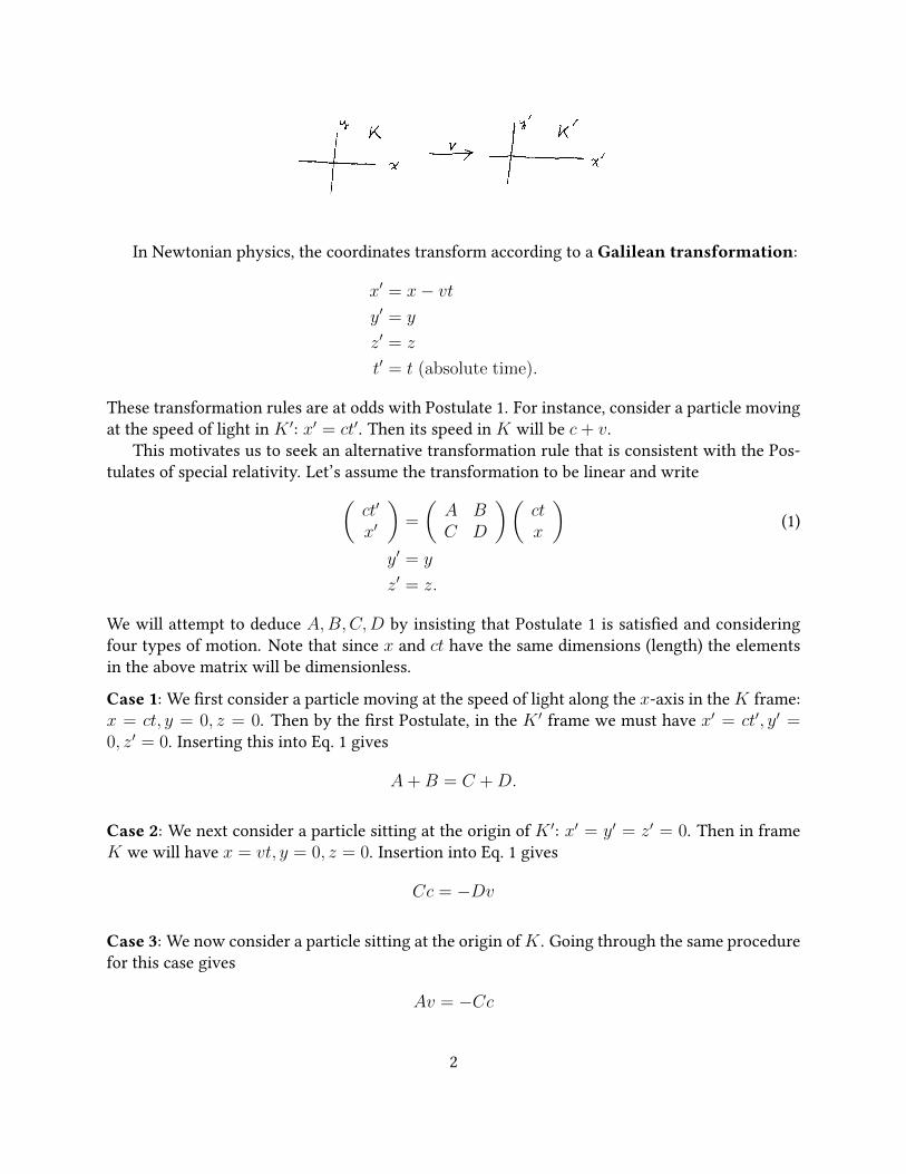
ferent reference frames. We take two reference frames K and K ′ as shown in the gure. Forconvenience we take the origins to coincide at time t = t′ = 0.

K coordinates : r = (x, y, z) and t

K ′ coordinates : r′ = (x′, y′, z′) and t′

1Please send any comments or corrections to r.barnett (at) imperial.ac.uk.

1

Lecture 1 (13/1/14)

1

In Newtonian physics, the coordinates transform according to a Galilean transformation:

x′ = x− vty′ = y

z′ = z

t′ = t (absolute time).

These transformation rules are at odds with Postulate 1. For instance, consider a particle movingat the speed of light in K ′: x′ = ct′. Then its speed in K will be c+ v.

This motivates us to seek an alternative transformation rule that is consistent with the Pos-tulates of special relativity. Let’s assume the transformation to be linear and write(

ct′

x′

)=

(A BC D

)(ctx

)(1)

y′ = y

z′ = z.

We will attempt to deduce A,B,C,D by insisting that Postulate 1 is satised and consideringfour types of motion. Note that since x and ct have the same dimensions (length) the elementsin the above matrix will be dimensionless.

Case 1: We rst consider a particle moving at the speed of light along the x-axis in the K frame:x = ct, y = 0, z = 0. Then by the rst Postulate, in the K ′ frame we must have x′ = ct′, y′ =0, z′ = 0. Inserting this into Eq. 1 gives

A+B = C +D.

Case 2: We next consider a particle sitting at the origin of K ′: x′ = y′ = z′ = 0. Then in frameK we will have x = vt, y = 0, z = 0. Insertion into Eq. 1 gives

Cc = −Dv

Case 3: We now consider a particle sitting at the origin ofK . Going through the same procedurefor this case gives

Av = −Cc

2

Case 4: Finally, we consider a particle moving along the y-axis in K at the speed of light: x =

0, y = ct, z = 0. Postulate 1 requires(dx′

dt′

)2+(dy′

dt′

)2

= c2, z′ = 0. With Eq. 1 we nd

A2 = 1 + C2.

The equations for these four Cases can be solved to determine A,B,C,D. The solution givesct′

x′

y′

z′

=

γ −v

cγ 0 0

−vcγ γ 0 0

0 0 1 00 0 0 1

ctxyz

(2)

where

γ =1√

1− (v/c)2.

We have arrived at a Lorentz transformation. We will refer to γ as the relativistic factor. Arotation-free Lorentz transformation (as in the above) is a Lorentz boost.

One can verify that the inverse transformation (from K ′ to K) can be obtained by replacingv → −v. That is, (

ctx

)=

(γ v

cγ

vcγ γ

)(ct′

x′

)(3)

with y = y′, z = z′.Special relativity forces us to abandon the notion of absolute time, and to consider four-

dimensional spacetime. A point (ct, x, y, z) in spacetime is called an event.

1.2 Some Consequences of the Lorentz Transformation1.2.1 Simultaneity

In Newtonian physics, events simultaneous in one frame are simultaneous in another. Wewill now illustrate how things are dierent in special relativity.

4

Lecture 2 (14/1/14)

4

3

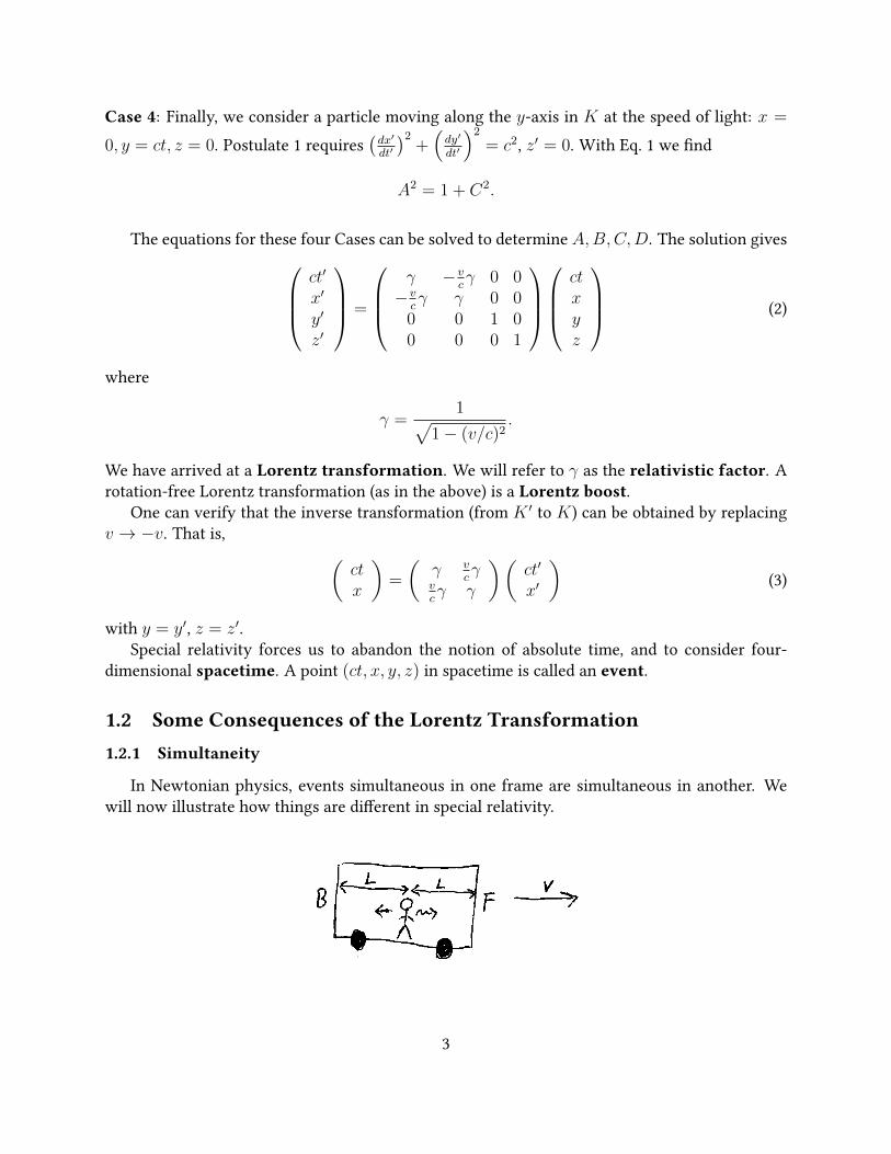
Consider a passenger standing in the middle of a train car which is moving at velocity v asshown in the picture. The person emits a pulse of light at time t′ = 0. We will consider the timeit takes for the pulse to reach the front and back of the train in dierent reference frames. Wetake K ′ to be the rest frame of the train. Then

x′F = L, x′B = −L, t′F = t′B = L/c

∆t′ = t′F − t′B = 0 (Simultaneous in K ′)

In this subscripts F,B denote the front and back of the train. For instance, t′F is the time in K ′at which the light reaches the front of the train. On the other hand, in K (the platform frame)through the Lorentz transformation we have

tF = γ(t′F + x′Fv/c2) =

γL

c

(1 +

v

c

), tB = γ(t′B + x′Bv/c

2) =γL

c

(1− v

c

)∆t = tF − tB = 2γ

Lv

c2(Not simultaneous in K ′)

Lecture 3 (18 Jan)

1.2.2 Time Dilation

Consider a clock sitting at the origin in K ′. The time intervals in K and K ′ are related by theLorentz transformation:

∆t = γ(∆t′ +v

c2∆x′) = γ∆t′

(∆x′ = 0 since the clock is motionless in K ′). The time recorded by a clock in its rest frame isreferred to as the proper time τ and so

∆τ = ∆t/γ

Since γ > 1 (for v 6= 0) the time interval in K is longer: “Moving clocks run slowly”. Thisphenomenon is known as time dilation.

1.2.3 Length Contraction

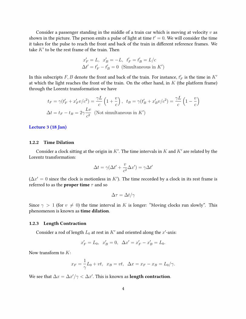
Consider a rod of length L0 at rest in K ′ and oriented along the x′-axis:

x′F = L0, x′B = 0, ∆x′ = x′F − x′B = L0.

Now transform to K :

xF =1

γL0 + vt, xB = vt, ∆x = xF − xB = L0/γ.

We see that ∆x = ∆x′/γ < ∆x′. This is known as length contraction.

4

6

7

1.3 Relativistic Addition of VelocitiesConsider a particle moving at velocity w in K ′: dx′/dt′ = w. What is the particle’s velocity

u = dx/dt as measured in K? In Newtonian physics, the result is

u = v + w.

On the other hand, by taking the dierential of the Lorentz transformation, we have

dx = γ(dx′ + vdt′) = γdt′(w + v)

dt = γ(dt′ + vdx′/c2) = γdt′(1 + vw/c2).

Dividing these equations gives

u =dx

dt=

v + w

1 + vwc2

. (4)

This gives the correct way to add velocities in special relativity. In comparing this with theNewtonian result, we see that the denominator serves to enforce the speed limit of light. Notethat this formula will be modied if the particle is not moving along the x′-axis. As our derivationdid not rely on w being constant, Eq. 4 is true even if the particle in K ′ is accelerating.

Eq. 4 can also be arrived at by considering a combination of Lorentz boosts. Take referenceframe K and K ′ to be as before. Now consider a third frame K ′′ in which the particle discussedpreviously is at rest. That is, the origin of K ′′ is moving away from the origin of K ′ at velocityw along the x′-axis. Now dene the rapidity ψv through

v

c= tanh(ψv)

with analogous relations for ψu and ψv.Then the matrix which transforms or “boosts” (ct, x) to (ct′, x′) is (compare to Eq. 2)

λ(v) ≡(

γ −γ vc

−γ vc

γ

)=

(cosh(ψv) − sinh(ψv)− sinh(ψv) cosh(ψv)

)= e−σψv (5)

5

where σ =

(0 11 0

)(check). In this we take the exponential of a square matrix A to be dened

through eA =∑∞

n=0An

n!. Writing the Lorentz boost in such a way enables us to nd a simple way

to evaluate combinations of boosts. The boost from K to K ′′ is given by

λ(u) = e−σψu = λ(w)λ(v) = e−σψwe−σψv = e−σ(ψw+ψv).

Thus the rapidities combine in a simple way:

ψu = ψv + ψw. (6)

Eq. 4 can be deduced from Eq. 6 (check).

Lecture 4 (19 Jan)

1.4 Relativistic AccelerationNow we move on to nd how to transform a particle’s acceleration between inertial reference

frames. We start by taking the dierential of Eq. 4 (recall that u = dx/dt and w = dx′/dt′):

du =1

γ2

1

(1 + vwc2

)2dw.

Next, take the dierential of an equation from our Lorentz transformation:

dt = γ(dt′ +v

c2dx′) = γ(1 +

vw

c2)dt′.

Dividing these equations gives

du

dt=d2x

dt2=

1

γ3

1(1 + vw

c2

)3

d2x′

dt′2

which relates d2xdt2

and d2x′

dt′2.

Example: The relativistic rocket. We consider a passenger aboard a rocket who always“feels” a constant acceleration a = d2x′

dt′2(i.e./ the acceleartion as measured from a MCF).

What is the rocket’s velocity u(t) measured in the K frame?We take the inertial frameK ′ to be moving away from the origin ofK with the same speedas the rocket at a particular time (a momentarily comoving frame – more on this later).Then at this particular time, u = v and w = 0. This gives a dierential equation for u:

du

dt=

(1−

(uc

)2)3/2

a.

6

For simplicity, let’s assume the rocket starts from rest: u(0) = 0. Solving this dierentialequation gives

u(t) =at√

1 +(atc

)2.

This expression gives very sensible results in limiting cases. For short times, u ≈ at as inNewtonian physics, while for long times, u ≈ c.

1.5 Relativistic Energy and MomentumWe now move on to generalise the familiar expressions of energy and momentum from New-

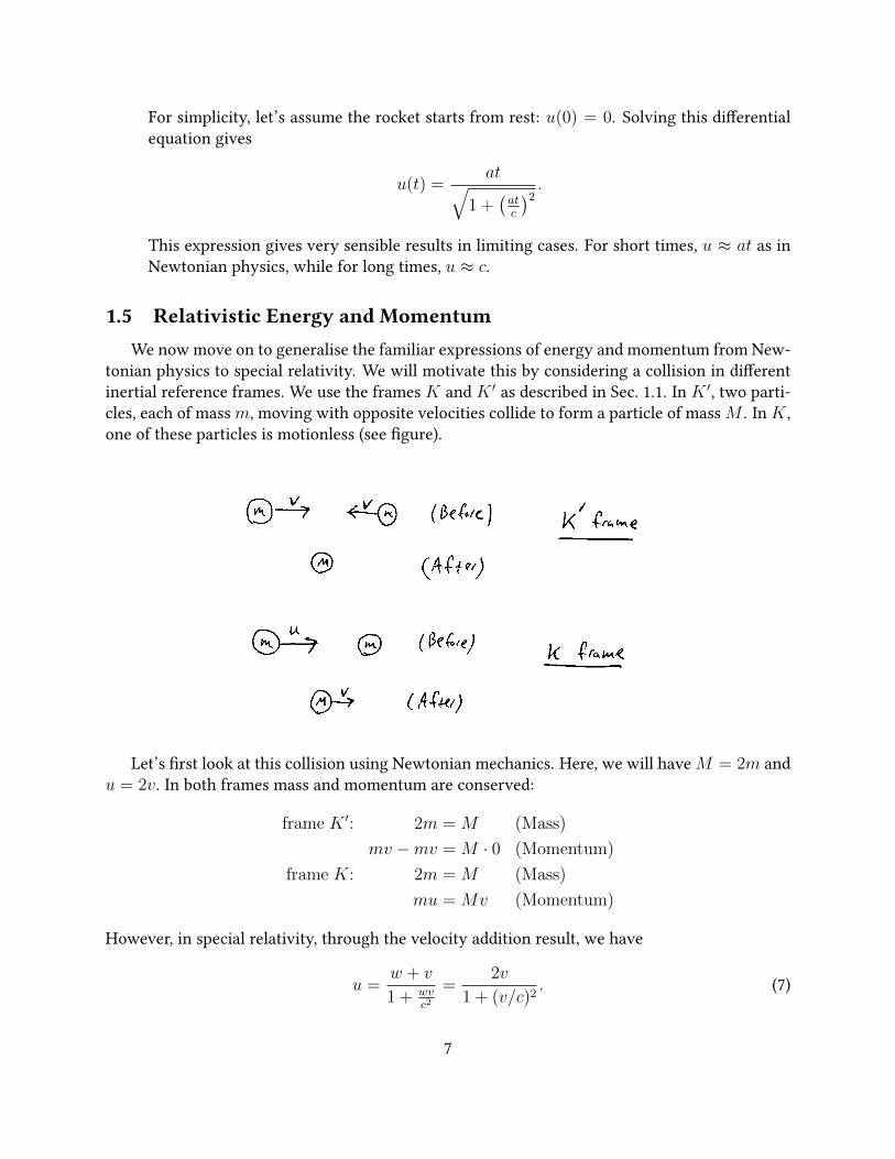
tonian physics to special relativity. We will motivate this by considering a collision in dierentinertial reference frames. We use the frames K and K ′ as described in Sec. 1.1. In K ′, two parti-cles, each of mass m, moving with opposite velocities collide to form a particle of mass M . In K ,one of these particles is motionless (see gure).

Let’s rst look at this collision using Newtonian mechanics. Here, we will have M = 2m andu = 2v. In both frames mass and momentum are conserved:

frame K ′: 2m = M (Mass)

mv −mv = M · 0 (Momentum)

frame K: 2m = M (Mass)

mu = Mv (Momentum)

However, in special relativity, through the velocity addition result, we have

u =w + v

1 + wvc2

=2v

1 + (v/c)2. (7)

7

With this, the Newtonian momentum conservation equation in K does not hold: mu 6= Mv.This motivates us to consider the case where mass depends on velocity by the replacement

m → f(v)m where f(v) is some function to be determined. With this replacement and takingf(0) = 1 we have

frame K ′: 2mf(v) = M (Mass)

f(v)mv − f(v)mv = M · 0 (Momentum)

frame K: mf(u) +m = Mf(v) (Mass)

mf(u)u = Mf(v)v (Momentum)

Solving the equations in K for f(u) gives f(u) = v/(u − v). Combining this with Eq. 7 givesf(u) = 1/

√1− (u/c)2. So we see that f(u) is nothing other than the relativistic factor: f(u) =

γ(u).We should check that all these equations are satised with this choice for f . This is easiest

to do by utilising the rapidities introduced earlier. Here we will have ψu = ψv + ψv = 2ψv. Themass equation in frame K ′ gives M = 2m cosh(ψu/2).2 Inserting this value into the equationsin K we nd the following identities:

cosh(ψu) + 1 = 2 cosh2(ψu/2)

sinh(ψu) = 2 sinh(ψu/2) cosh(ψu/2)

so everything checks.We say a particle with rest massm moving at velocity v has a relativistic mass γ(v)m. We

further dene the relativistic momentum to be p = γ(v)mv. Extending this to several componentswe have

p = γ(v)mv (8)

where v = dr/dt. With these revised expressions, we have that momentum and mass are con-served in the above collision. We further interpret the conservation of mass as conservation ofenergy. Multiplying the relativistic mass by c2 (to obtain correct units) we dene the relativisticenergy to be

E = γ(v)mc2. (9)

This interpretation becomes quite plausible for v/c 1. In this regime we have

E ≈ mc2 +1

2mv2.

The second term in the above is the Newtonian kinetic energy.

Lecture 5 (22 Jan)

2Note that the relativistic factor of a particle moving at velocity v is γ(v) = cosh(ψv)

8

1.6 A More Systematic NotationWe will now introduce some terminology and a more systematic notation which will be used

in general relativity. We label spacetime coordinates as follows:

x0 = ct x1 = x x2 = y x3 = z

(the superscripts here are not to be confused with exponents). We thus label an event by3

xµ = (ct, x, y, z) = (ct, r).

It also proves convenient to use the Einstein summation convention. With this convention,summation is implied in an expression when an index appears twice. For instance,

XµYµ ≡3∑

µ=0

XµYµ = X0Y0 + . . .+X3Y3.

We will later discuss the relevance of superscript and subscript indices. Suppression of the sum-mation symbol often proves to be economical, but we must be careful not to write ambiguousexpressions.4

We next introduce the Minkowski metric:

ηµν =

1 0 0 00 −1 0 00 0 −1 00 0 0 −1

. (10)

This gives us a way of taking “dot products” of spacetime vectors. The spacetime line element dsis dened through

(ds)2 = ηµνdxµdxν = c2(dt)2 − (dx)2 − (dy)2 − (dz)2 (11)

which is analogous to dr · dr in Euclidean space. Let’s consider how (ds)2 changes under ourLorentz boost Eq. 2:

(cdt)2 − (dx)2 = γ2(cdt′ + vdx′/c)2 − γ2(dx′ + vdt′)2

= γ2(c2 − v2)(dt′)2 − γ2(1− (v/c)2)(dx′)2

= c2(dt′)2 − (dx′)2.

Since y = y′ and z = z′, we therefore have

(ds)2 = ηµνdxµdxν = ηµ′ν′dx

µ′dxν′. (12)

3This equation may appear a little sloppy. Strictly speaking, xµ are the components of the spacetime point. Suchexpressions are common in GR.

4For instance, we might be tempted to write (XµYµ)2 = XµYµX

µYµ but this in not correct. Instead, we needto introduce another index: (XµYµ)

2 = XµYµXνYν .

9

The line element is invariant under our Lorentz transformation. In fact (ds)2 is invariant underall Lorentz transformations (think about, say, boosts in the y and z directions). In Eq. 12 we haveplaced primes on indices to denote that these quantities are in the K ′ reference frame. This isknown as the kernel-index convention.

Now let’s introduce a more compact notation for Lorentz transformations:

dxµ′= Λµ′

νdxν .

For instance, for the Lorentz transformation we have been regularly using, Λµ′ν is the matrix

appearing in Eq. 2. Inserting this into the spacetime line element and demanding that this quantityis invariant gives

ηµν = Λσ′

µησ′ρ′Λρ′

ν (13)

or in matrix form

η = ΛTηΛ. (14)

We take this condition as the dening relation for Lorentz transformations. More precisely, thea transformation dxµ

′= Λµ′

νdxν is a Lorentz transformation if and only if Λ satises Eq. 13.

It can be veried that the collection of matrices satisfying Eq. 14 form a group under matrixmultiplication. This group is known as the Lorentz group.

Lecture 6 (25 Jan)

Suppose that two vectors transform under a Lorentz transformation as Xµ′ = Λµ′νX

ν andY µ′ = Λµ′

νYν . By using Eq. 14 it follows that

XµY νηµν = Xµ′Y ν′ηµ′ν′ .

So we see that this “dot product” is invariant. This is analogous to the way the dot product of twoCartesian vectors is invariant when they are rotated about the origin, since rotation matrices areorthogonal. However, unlike Cartesian vectors, the dot product ofXµ with itself can be negative.Xµ is a timelike, spacelike, or null vector ifXµXνηµν is positive, negative, or zero respectively.

1.7 Momentarily Comoving Reference FrameFor a particle moving at constant velocity, we can transform to an inertial frame in which

the particle is always at rest. What about an accelerating particle? For this, we introduce theMomentarily Comoving Frame (MCF) which is an inertial frame in which the particle is mo-mentarily at rest. Let’s revisit the line element (ds)2. Let K ′ be a MCF of the particle. Then atthe moment the particle is at rest we have

(ds)2 = c2(dt)2 − (dx)2 − (dy)2 − (dz)2 = c2(dt′)2 − (dx′)2 − (dz′)2 = c2(dt′)2 = c2(dτ)2

10

where dτ is the dierential of the particle’s proper time (the proper time is the time a clocktravelling with the particle would keep). So we have the important relation

(ds)2 = c2(dτ)2. (15)

This holds even if the particle is accelerating.Let’s revisit time dilation. We can rewrite Eq. 15 as

(c2 − v2)(dt)2 = c2(dτ)2

where v2 = drdt· drdt

. Then we can compute a proper time interval as

∆τ =

∫ tf

ti

dt√

1− (v/c)2

where ti and tf denote the initial and nal times in frameK . Note that this reduces to our previousresult ∆τ = ∆t/γ when v is constant.

1.8 Four-Velocity and Four-MomentumDividing Eq. 15 by (dτ)2 we obtain

uµuνηµν = c2

where

uµ =dxµ

dτ.

is the four-velocity. The four-momentum of a massive particle is dened as

pµ = mdxµ

dτ.

Note that pµpνηµν = m2c2. We see that these are both timelike vectors.Since dxµ′ = Λµ′

νdxν and dτ is invariant, we have that the four-velocity and four-momentum

transform simply under a Lorentz transformation: uµ′ = Λµ′νu

ν , pµ′ = Λµ′νpν . This is a primary

reason for why it is often best to work with these four vectors. Note, for instance, that thecoordinate velocity dr/dt does not transform in such a simple way.

Consider a particle moving with velocity v along the x-axis ofK . Now let’s consider boostingto a MCF. In this frame, all components except for the 0-component of pµ′ will be zero. Using Eq.15 we nd

pµ′= (mc, 0, 0, 0).

Next, let’s transform back to K :

pµ = (γmc, γmv, 0, 0) = (E/c, p, 0, 0)

11

where p = γmdx/dt is the relativistic momentum introduced earlier.The above argument can be repeated for a particle moving in an arbitrary direction. One nds

pµ = (E/c,p). (16)

For the four-velocity, one similarly nds

uµ = (γc, γv). (17)

The four-momentum is very useful since it combines our conserved quantities into a single vector.Conservation of energy and momentum can be expressed simply as

dpµ

dτ= 0.

Inserting Eq. 16 into our condition pµpνηµν = m2c2 gives an expression for the relativisticenergy

E =√

(mc2)2 + (pc)2 (18)

(compare to Eq. 9). For pcmc2 1 we have

E ≈ mc2 +p2

2m

where the second term, again, is the Newtonian kinetic energy.

Lecture 7 (26 Jan)

1.9 Photons and the Doppler EectPhotons are particles (or quanta) of light. They have zero mass. From Eq. 18, we see that we

can express the energy of a photon as E = pc. Using Eq. 16, we see that

pµpνηµν = 0.

So the four-momentum of a photon is a null vector. Also, by considering Eq. 17, we see that thefour-velocity of a photon is ill-dened (instead we take a m → 0, v → c limiting case of thefour-momentum).

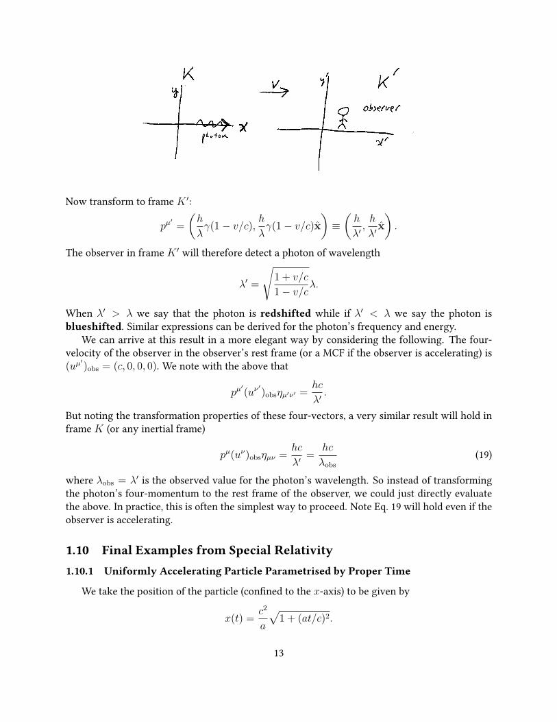
Borrowing a basic result from modern physics, the energy of a photon is given by E = hνwhere h is Planck’s constant and ν is the photon’s frequency (units of inverse time). The photon’swavelength λ satises λν = c. How does the photon’s wavelength change when viewed from adierent reference frame (as shown in the drawing)?

In frame K , the photon’s four-momentum is

pµ = (E/c,p) =

(h

λ,h

λx

).

12

Lecture 5 (21/1/14)

19 20

Now transform to frame K ′:

pµ′=

(h

λγ(1− v/c), h

λγ(1− v/c)x

)≡(h

λ′,h

λ′x

).

The observer in frame K ′ will therefore detect a photon of wavelength

λ′ =

√1 + v/c

1− v/cλ.

When λ′ > λ we say that the photon is redshifted while if λ′ < λ we say the photon isblueshifted. Similar expressions can be derived for the photon’s frequency and energy.

We can arrive at this result in a more elegant way by considering the following. The four-velocity of the observer in the observer’s rest frame (or a MCF if the observer is accelerating) is(uµ

′)obs = (c, 0, 0, 0). We note with the above that

pµ′(uν

′)obsηµ′ν′ =

hc

λ′.

But noting the transformation properties of these four-vectors, a very similar result will hold inframe K (or any inertial frame)

pµ(uν)obsηµν =hc

λ′=

hc

λobs

(19)

where λobs = λ′ is the observed value for the photon’s wavelength. So instead of transformingthe photon’s four-momentum to the rest frame of the observer, we could just directly evaluatethe above. In practice, this is often the simplest way to proceed. Note Eq. 19 will hold even if theobserver is accelerating.

1.10 Final Examples from Special Relativity1.10.1 Uniformly Accelerating Particle Parametrised by Proper Time

We take the position of the particle (conned to the x-axis) to be given by

x(t) =c2

a

√1 + (at/c)2.

13

Note that dxdt

= at√1+(at/c)2

gives the result we found previously for the relativistic rocket. Using(ds)2 = c2(dτ)2 we nd

c2(dτ)2 = c2(dt)2 − (dx)2 =c2

1 + (at/c)2(dt)2.

So

τ =

∫dt√

1 + (at/c)2=c

asinh−1(at/c) + const.

Setting the integration constant to zero so that τ = 0 when t = 0, we nd that the particle’strajectory or world line parametrised by τ is given by

xµ =

(c2

asinh(aτ/c),

c2

acosh(aτ/c), 0, 0

).

As a check, we can evaluate the particle’s four-velocity and verify uµuνηµν = c2.

Lecture 8 (29 Jan)

1.10.2 Rindler Coordinates

Up until now, we have been treating the rocket essentially as a point particle. Our aim hereis to nd a coordinate system which is glued to the moving rocket (do not worry if this exampleis confusing at rst or second pass). We continue to take all motion to be conned to the x-axis.

First, let’s consider the following: suppose that we take all components of the rocket to beaccelerating with the same uniform acceleration. For instance, we take the trajectory of the frontand back of the rocket to be given by

xF (t) =c2

a

√1 + (at/c)2 +

(xF −

c2

a

)xB(t) =

c2

a

√1 + (at/c)2 +

(xB −

c2

a

)so that at t = 0, xF = xF and xB = xB . By dierentiating these relations, we nd the expectedresults for uniform acceleration. Now we note that at all times the rocket will have the same lengthxF (t)− xB(t) = xF − xB in the K frame. But from our considerations of length contraction, weexpect that this rocket will be stretched out in its rest frame (if we can dene such a thing!).

We instead seek a way to accelerate the rocket as a rigid object. First, let’s consider thetrajectory from the previous example: x(t) = c2

a

√1 + (at/c)2. This satises

x2 − c2t2 = X2a

where Xa ≡ c2/a. Through our Lorentz transformation we also nd

x′2 − c2t′2 = X2a . (20)

14

Now consider the following. Take the front and back of the rocket to have dierent uniformaccelerations with aF < aB (so that it maintains a constant rest length we want to accelerate thefront less than the back). Let’s further take the trajectories of the front and back to be given by

x2F − c2t2 =

(c2

aF

)2

= X2aF

x2B − c2t2 =

(c2

aB

)2

= X2aB.

Then at t = 0 both front and back ends of the rocket will be at rest with xF = XaF , xB = XaB ,and xF − xB = XaF − XaB . Now consider transforming to frame K ′ through Eq. 20. At timet′ = 0, we see that the rocket is at rest in this frame and will have the same rest length: x′F = XaF ,x′B = XaB , and x′F − x′B = XaF −XaB . Thus, we have found a way to accelerate the front andback of the rocket so that the the rest length of the rocket is xed. In fact, we can determine theacceleration of any intermediate point within the rocket in such a way. For instance the centreof the rocket will accelerate with uniform acceleration aC given by 1/aC = (1/aF + 1/aB) /2.

With such considerations, we see that the family of trajectories

x2 − c2t2 = X2 (21)

(for dierent X values) will describe how to accelerate the rocket as a rigid object. Additionally,X will give the position in a coordinate system glued to the accelerating rocket. From X = c2/awe can read o how fast we need to accelerate this point so that the whole rocket accelerates asa rigid object.

We therefore take X to label position in the rocket’s frame. What about time? Eq. 21 issuggestive. Suppose we choose a time coordinate T such that

t =1

cX sinh(aBT/c).

Then x = X cosh(aBT/c) (this satises Eq. 21). From the previous example, we identify T asthe time kept by a clock sitting at the back of the rocket. This is a sensible time coordinate butwe could have put the clock somewhere else in the rocket. Note that clocks sitting at dierentpositions in the rocket will tick at dierent rates. X and T are called Rindler coordinates.

For a massive particle under no external forces we have dpµ/dτ = 0 in an inertial frame. Inthe Rindler Coordinate system this reads (with some work)

d2T

dτ 2+

2

X

dX

dτ

dT

dτ= 0

d2X

dτ 2+(aBc

)2

X

(dT

dτ

)2

= 0.

Solving these equations would give, say, the trajectory of a ball dropped in the rocket as seenfrom inside the rocket. The ball will fall as if it is under a gravitational eld. In our investigation

15

of general relativity, we will look at similar systems of equations in non-inertial reference frameswith one important dierence: unlike the above, the gravitational elds in GR cannot be removedeverywhere with a coordinate transformation.

This completes our overview of special relativity.5

5There’s a neat game which allows you to “experience” special relativity including Lorentz contractions andred/blue shifts at http://gamelab.mit.edu/games/a-slower-speed-of-light/.

16

2 Mathematics of General Relativity

2.1 The Equivalence Principle and What’s Ahead

Lecture 9 (1 Feb)

Let’s consider the following thought experiment. Consider two lifts. One is deep in outerspace, while the other is freely falling under the earth’s gravitational eld. A passenger is aboardone of the two lifts. By doing experiments over small regions of spacetime the passenger cannotdiscern between the two scenarios. That is, the passenger would feel weightless in both lifts. Thepassenger could do local kinematic experiments and observe that Newton’s rst law is obeyed foreither case.6 This is due to the equivalence of gravitational and inertial mass. This is summarisedby the equivalence principle:

• In a freely falling laboratory occupying a small region of spacetime, special relativity holds.

When gravitational elds are present, it is generally not possible to nd a coordinate systemwhich is inertial everywhere. In general relativity, gravity is accounted for by the curvature ofspacetime. Free particles follow the straightest possible paths in this curved spacetime. From ourdiscussion of special relativity, we have the line element and the equations of motion of a massiveparticle under no forces are given by

(ds)2 = ηµνdxµdxν ,

d2xµ

dτ 2= 0.

We will nd that these equations generalise to

(ds)2 = gµνdxµdxν ,

d2xµ

dτ 2+ Γµνσ

dxν

dτ

dxσ

dτ= 0

(gµν and Γµνσ to be dened soon).

2.2 General Coordinate Systems for Euclidean spaceBefore jumping into our discussion of dierentiable manifolds, we will start with something

more familiar: three-dimensional Euclidean space. We will nd that many of the results fromEuclidean space will carry over naturally to the general case. We will start labeling indices withletters near the beginning of the alphabet a, b, c, d, . . . (hopefully we will not need to go too farinto the alphabet!). We will reserve Greek indices for spacetime.

6On the other hand, over larger regions of spacetime the passenger would be able to discern between the twolifts. For instance, if the lift is falling under the earth’s gravitational eld, since the gravitational eld is radial, thehorizontal distance between two balls released from rest from the left and right hands of the passenger will eventuallydecrease in apparent violation of Newton’s rst law. The balls would keep a constant horizontal separation for thelift deep in space.

17

2.2.1 General Basis Vectors

Let

(x, y, z) = (x1, x2, x3)

be the usual Cartesian coordinates and

(u, v, w) = (u1, u2, u3)

be an arbitrary coordinate system. We will restrict our attention to cases where the Cartesiancoordinates can be written as functions of the (u, v, w) coordinates and vice versa. Write

r = x(u, v, w)x + y(u, v, w)y + z(u, v, w)z

and consider the vectors

e1 =∂r

∂u, e2 =

∂r

∂v, e3 =

∂r

∂w

or, more succinctly,

ea =∂r

∂ua.

These vectors are not necessarily mutually orthogonal or normalised. Now consider anothercollection of vectors dened by

e1 = ∇u, e2 = ∇v, e3 = ∇w

or ea = ∇ua. In this,∇ = x ∂∂x

+ y ∂∂y

+ z ∂∂z

is the usual gradient operator. Note we need to writethe ua coordinates as functions of the Cartesian coordinates to evaluate the above.

We will now establish a useful relationship between these vectors:

ea · eb = ∇ua · ∂r∂ub

=∂ua

∂x

∂x

∂ub+∂ua

∂y

∂y

∂ub+∂ua

∂z

∂z

∂ub=∂ua

∂xc∂xc

∂ub=∂ua

∂ub

In these manipulations, we have made use of the chain rule. We have found the orthogonalityrelation

ea · eb = δab

where δab is the Kronecker delta function: δab = 1 if a = b, δab = 0 if a 6= b. This orthogonalityrelation can be used to establish the linear independence of e1, e2, e3. That is, consider c1, c2, c3

which satisfy

c1e1 + c2e

2 + c3e3 = 0.

18

Taking the dot product of this equation with ea, and using the orthogonality relation will givec1 = c2 = c3 = 0. A similar argument can be used to establish that e1, e2, e3 are linearlyindependent. We will call e1, e2, e3 the natural basis and e1, e2, e3 the dual basis.

A general vector X in Euclidean space can therefore be written in either basis:

X = Xaea = Xaea.

(summation implicit). We call Xa the contravariant components of X and Xa the covariantcomponents of X. Using this orthogonality relation, the components of X can be extracted as:

ea ·X = ea ·Xbeb = Xbδ

ba = Xa.

Similarly, Xa = ea ·X.

2.2.2 The Metric

We dene the metric gab as

gab = ea · eb.

Similarly, we dene gab = ea · eb. From these denitions, we see that these quantities are sym-metric: gab = gba, gab = gba. Now consider two arbitrary vectors, X and Y which can be writtenas

X = Xaea = Xaea

Y = Y aea = Yaea.

There are four ways we can write the dot product of these vectors:

X ·Y = gabXaY b = gabXaYb = XaYa = XaY

a.

Let’s consider XaYa = gabXaYb. Since this is true for arbitrary X, it must be that

Y a = gabYb.

Similarly, XaYa = gabXaY b tells us that

Ya = gabYb.

We see that the metric can be used to convert contravariant to covariant components and viceversa. We also have for arbitrary Y a,

Y a = gabYb = gabgbcYc.

Therefore,

gabgbc = δac .

That is, gab is the inverse of gab.

Lecture 10 (2 Feb)

19

Example: Cylindrical coordinates. Let’s apply what we have established so far to cylindri-cal coordinates. We take u = ρ, w = φ, and v = z where x = ρ cos(φ), y = ρ sin(φ). Wend (check)

e1 = cos(φ)x + sin(φ)y

e2 = −ρ sin(φ)x + ρ cos(φ)y

e3 = z

e1 = cos(φ)x + sin(φ)y

e2 = −1

ρsin(φ)x +

1

ρcos(φ)y

e3 = z

and

gab = diag(1, ρ2, 1), gab = diag(1,1

ρ2, 1).

2.2.3 Why Do We Need Two Types of Basis Vectors?

Why do we need two types of basis vectors? First we note that if (u, v, w) are just the Cartesiancoordinates, then the natural basis and the dual basis are the same: x = e1 = e1 with similarrelations for the y and z basis vectors. For the Cartesian basis, we will use the notation x = x1 =x1 with similar relations for the other vectors.

Now let’s go back to arbitrary (u, v, w). Some quantities are most naturally described by thedual basis. For instance, consider a scalar function f(u, v, w). The gradient of this is

∇f =∂f

∂xaxa =

∂f

∂ub∂ub

∂xaxa =

∂f

∂uaea.

So we see that gradients are naturally expressed in the dual basis.On the other hand, some quantities are better described by the natural basis. Suppose we have

a curve in Euclidean space parameterised by t: r(t) = x(t)x + y(t)y + z(t)z. A vector tangentto this curve is given by

dr

dt=

∂r

∂uadua

dt= uaea

where ua ≡ dua

dt. Thus tangent vectors to curves are expressed in terms of the natural basis.

2.2.4 Arc Length

Let’s take the curve parametrised by t from the previous section and restrict t to a ≤ t ≤ b.Using our machinery, we see that the arc length ` of this curve is

` =

∫ a

b

dt

√dr

dt· drdt

=

∫ a

b

dt√uaubgab.

20

Example: Arc length of spiral. Let’s consider a curve which is naturally described in cylin-drical coordinates. Take a spiral with ρ = R = const, φ = t, z = t, and 0 ≤ t ≤ T . Then,using the metric from the previous example we nd (check)

` =

∫ T

0

dt

√g11ρ2 + g22φ2 + g33z2 = T

√1 +R2.

2.2.5 Coordinate Transformations

We will now introduce another arbitrary coordinate system (u′, v′, w′) and consider how totransform quantities between this and the (u, v, w) coordinate system. We will refer to these asthe primed and unprimed coordinate systems. In the primed coordinate system, we nd basisvectors using the same procedure as before: ea′ = ∂r

∂ua′and ea

′= ∇ua′ . Using the chain rule, we

can nd how the basis vectors transform under a change of coordinates:

ea =∂r

∂ua=

∂r

∂ub′∂ub

′

∂ua= J b

′

a eb′

where J b′a = ∂ub′

∂uais the Jacobian matrix. In a similar way, we can nd the transformation rule

for ea:

ea = ∇ua =∂ua

∂xbxb =

∂ua

∂uc′∂uc

′

∂xbxb = Jac′e

c′ = Jab′eb′ .

With these coordinate systems, there are multiple ways to write a vector X

X = Xaea = Xaea = Xa′ea′ = Xa′e

a′ .

Inserting the transformation rules for the basis vectors into the above determines how the com-ponents of X transform. One nds

Xa′ = Ja′

b Xb and Xa′ = J ba′Xb. (22)

Finally, we note that the chain rule gives a useful result:

Jac′Jc′

b =∂ua

∂uc′∂uc

′

∂ub=∂ua

∂ub= δab .

Lecture 11 (5 Feb)

2.3 Surfaces in Euclidean SpaceWe will now consider surfaces in three-dimensional Euclidean space. Most of the results for

Euclidean space established previously can be seen to carry over to this case. We take the surfaceto be given parametrically by

r(u, v) = x(u, v)x + y(u, v)y + z(u, v)z.

21

As before, we obtain the natural basis vectors e1 = ∂r∂u

and e2 = ∂r∂v

. These vectors evaluatedat a particular point P on the surface are tangent to the surface at this point. The collection ofvectors tangent to the surface at P form a vector space which we denote as TP . Our vectors e1

and e2 can be taken as a basis for this tangent space.As before, we dene the metric as gab = ea·eb. We take gab to be the inverse of gab: gacgcb = δab .

Finally we take ea = gabeb (note the diculty in dening ea as we did in the previous section).Note with this ea · eb = gacec · eb = gacgcb = δab .

Example: The unit sphere. We take the unit sphere to be parametrised by θ = u = u1,φ = v = u2 as

r(θ, φ) = sin(θ) cos(φ)x + sin(θ) sin(φ)y + cos(θ)z.

By dierentiating this expression we have

e1 = cos(θ) cos(φ)x + cos(θ) sin(φ)y − sin(θ)z

e2 = − sin(θ) sin(φ)x + sin(θ) cos(φ)y

With these, we can evaluate the metric. The line element can be found to be

(ds)2 = dr · dr = gabduadub = (dθ)2 + sin2(θ)(dφ)2.

2.4 General Tensors and ManifoldsEuclidean space and two-dimensional surfaces in Euclidean space are both examples of a

more general entity called a manifold. An N -dimensional manifold is a space which is locallyisomorphic to Euclidean space RN . For instance a small region about any point on the unit sphereis locally isomorphic to R2. Points on an N -dimensional manifold are labelled by N coordinates(x1, x2, . . . , xN) in such a way that there is a one-to-one correspondence between points in themanifold and coordinate values. It is not generally possible to describe an entire manifold in sucha way with a single set of coordinates. Taking our example of the unit sphere, there is not a one-to-one correspondence between coordinate values and points in the manifold at the north andsouth poles of the sphere. That is, when θ = 0 or θ = π, all values of φ describe the same point.For such situations, one needs to use multiple coordinate systems to cover dierent regions ofthe manifold.

Suppose we have a region of a manifold described by two coordinate systems (x1, x2, . . . , xN)and (x1′ , x2′ , . . . , xN

′). Assuming the one-to-one correspondence described above, the xa coor-

dinates can be written as functions of the xa′ coordinates and vice versa. We can thus dene theJacobian matrices as before: Jab′ = ∂xa

∂xb′and Ja′b = ∂xa

′

∂xbwhich satisfy, through the chain rule,

Jab′Jb′c = δac . We carry over the transformation rules for contravariant and covariant vectors ar-

rived at earlier to the present case: given a contravariant vector Xa and a covariant vector Ya,we have Xa′ = Ja

′

b Xb and Ya′ = J ba′Yb.

7

7We are being loose with terminology here. Strictly speaking, Xa and Ya are components of vectors and notvectors. This distinction is commonly dropped in textbooks on GR. We will adopt this convention and refer to Xa

itself as a contravariant vector.

22

Contravariant and covariant vectors are examples of a more general quantity called a tensor.Suppose at a particular point in the manifold, we have Nn+m quantities that transform under achange of coordinates as

Ta′1...a

′n

b′1...b′m

= Ja′1

c1. . . Ja

′n

cn Jd1b′1. . . Jdmb′m T

c1...cnd1...dm

.

Then T a1...anb1...bmis a type (n,m) tensor. A tensor eld dened over some region of the manifold

associates a tensor of the same rank to every point in the region.We will only consider manifolds which have an associated metric gab (which are known as

Riemannian manifolds). We take the metric to be a type (0, 2) tensor eld. As before we takegab to be the inverse of gab. It can be shown (exercise) that gab is then a type (2, 0) tensor eld.As before, gab and gab can be used to raise and lower indices. For instance, for a (2, 0) tensorT ab, T abgbc = T ac (it can also be checked that these quantities have the correct transformationproperties). Also, we see that gab = δab .

Example: ion. Take T abc to be a type (1, 2) tensor. DeneRa = T bab =∑

b Tbab. The b indices

are said to be contracted. In another coordinate system,

Ra′ = T b′

a′b′ = J b′

c Jda′J

eb′T

cde = δecJ

da′T

cde = Jda′T

ede = Jda′Rd.

So we see that Ra is a tensor. Generally, one can obtain an (n − 1,m − 1) tensor from an(n,m) tensor through contraction.

23

Lecture 12 (8 Feb)

2.5 Calculus of Variations and GeodesicsIn relativity, particles follow geodesics. A geodesic is the generalisation of the notion of a

straight line to a curved manifold. In the following, we will learn how to compute geodesics.

2.5.1 Calculus of Variations

Suppose we want to nd curves on the manifold parametrised by t, xa(t), which extremise

S[xa] =

∫ t2

t1

dtL(xa, xa, t).

To do this write xa = xa + δxa where δxa(t1) = δxa(t2) = 0. We insert xa into S and expand inδxa. In order for xa to describe an extremum, the rst order term must vanish. To rst order inδxa, we have

S[xa] =

∫ t2

t1

dtL(xa + δxa, xa + δxa, t)

=

∫ t2

t1

dt

(L(xa, xa, t) +

∂L

∂xaδxa +

∂L

∂xaδxa).

Note that a summation over a is implied for the linear terms in δxa. Next, we integrate by partsto obtain

S[xa] = S[xa] +

∫ t2

t1

dt

(∂L

∂xa− d

dt

∂L

∂xa

)δxa.

We require the linear piece to vanish for arbitrary δxa. Therefore,∂L

∂xa=

d

dt

∂L

∂xa(23)

which are the Euler-Lagrange equations.

2.5.2 Geodesics

As we saw before, the length of a curve between two points P1 and P2 is

` =

∫ P2

P1

ds =

∫ t2

t1

dt√gabxaxb

The geodesics are given by the Euler-Lagrange equations of L =√gabxaxb. Before diving into

computing these, we introduce

K =1

2gabx

axb. (24)

24

Working with K is easier since it doesn’t involve square roots. For K we have

∂K

∂xa= L

∂L

∂xa

d

dt

∂K

∂xa=

d

dt

(L∂L

∂xa

)= s

∂L

∂xa+ L

d

dt

∂L

∂xa

since L = dsdt

= s. By the Euler-Lagrange equations for L we thus have

d

dt

∂K

∂xa=∂K

∂xa+ s

∂L

∂xa.

Now we note that we have the freedom to choose a convenient parametrisation of the curve. Ifwe choose it to be related to s as t = αs + β where α 6= 0 and β are constants, then s = 0.Our parameter t is then called an ane parameter. Choosing t to be an ane parameter, theEuler-Lagrange equations become

d

dt

∂K

∂xa=∂K

∂xa. (25)

This is the easiest way to proceed.Evaluating Eq. 25 with Eq. 24, gives (exercise)

xa + Γabcxbxc = 0 (26)

where

Γabc =1

2gad (∂cgbd + ∂bgcd − ∂dgbc) (27)

(we will begin using the shorthand ∂∂xa

= ∂a). We will call Eq. 26 the geodesic equation. Γabcis known as a Christoel symbol. From Eq. 27 we see that the Christoel symbols have thesymmetry Γabc = Γacb.

Example: Obtaining the Christoel symbols from the Euler-Lagrange equations. This ex-ample will present a trick for determining Christoel symbols which often proves to be themost ecient way of computing him. To be concrete, let’s focus on the case of the unitsphere. For this, we have

K =1

2

(θ2 + sin2(θ)φ2

).

The Euler-Lagrange equations are

θ − sin(θ) cos(θ)φ2 = 0

φ+ 2 cot(θ)θφ = 0.

25

By comparison with the geodesic equation, Eq. 26, we deduce that the only non-vanishingChristoel symbols are

Γθφφ = − sin(θ) cos(θ)

Γφθφ = Γφφθ = cot(θ).

We can check that direct evaluation of Eq. 27 gives the same results, but the method of thisexample is much less tedious. Also, note that we are writing Γθφφ instead of Γ1

22, etc. Thishelps us keep track of variables (was the x1 variable θ or φ?).

Lecture 13 (9 Feb)

2.5.3 Comparison with Newtonian Mechanics

In Lagrangian mechanics, Newton’s second law is arrived at through a variational princi-ple. The Lagrangian of a Newtonian particle under an external potential V is dened to be theparticle’s kinetic energy minus its potential energy V . For example, let’s consider a particle inone spatial dimension. Then the Lagrangian is L = 1

2mx2 − V (x). It is readily veried that the

Euler-Lagrange equations give Newton’s second law: mx = −∂V∂x

. Classical particles move inways which extremize the action S where S =

∫ t2t1dtL .

The results of the previous section have an interesting connection with classical mechanics.First note that K = 1

2drdt· drdt

= 12gabx

axb is the kinetic energy (and Lagrangian) of a unit-massparticle under no external forces moving on a manifold. Newton’s second law for this particlewill be given by the Euler-Lagrange equations for K , Eq. 26. Conservation of energy tells usthat for a solution of Eq. 26 we will have E = 1

2gabx

axb = const.8 E = 12(ds/dt)2 then tells us

that t is an ane parameter (s = 0). Thus the classical trajectories will also extremize the arclength. From this, we conclude that the allowable trajectories of the classical particle will followgeodesics of the manifold. The allowable curves traced out by classical particles on a manifoldare determined by the geometry of the manifold alone.

2.6 Parallel TransportLet’s start by considering surfaces in Euclidean space. Let XP be a vector tangent to the

surface at a particular point P . Now let xa(t) describe a curve on the manifold starting at pointP at t = 0. How can we move the vector along the curve, keeping it in the tangent space of themanifold along the curve, and also keeping it “as parallel as possible”? If our manifold was all of

8We can arrive at conservation of energy directly from the Euler-Lagrange equations. Taking the time derivativeof K ,

dK

dt=∂K

∂xaxa +

∂K

∂xaxa =

d

dt

(∂K

∂xa

)xa +

∂K

∂xaxa =

d

dt

(∂K

∂xaxa)

so ddt

(∂K∂xa x

a −K)= 0. We can verify that K = ∂K

∂xa xa −K .

26

Euclidean space (and not a surface) the answer is more or less clear: we take X to be the same atevery point along the curve. However, this cannot generally be accomplished for a surface sincedierent points along the curve will have dierent tangent spaces. Instead, we take our conditionfor parallel transport to be

P · dX(xa(t))

dt= 0 (28)

where P = eaea = eaea projects into the tangent space.9 Note that dea/dt need not be in the

tangent space. We also require that X always is in the tangent space along the curve: P ·X = X.From Eq. 28 one nds that

Xa + ΓabcXbxc = 0 (29)

where Γabc = ea · ∂bec.We need to check that Γabc is consistent with our previous denition. First we lower the a

superscript: Γabc = gadΓdbc = ea · ∂bec. Then using ∂aeb = ∂a∂br = ∂b∂ar = ∂bea one can verify

that

Γabc = ea · ∂bec =1

2(∂b(ea · ec) + ∂c(ea · eb)− ∂a(eb · ec))

=1

2(∂bgac + ∂cgab − ∂agbc) .

So

Γabc = gadΓdbc =1

2gab (∂cgbd + ∂bgcd − ∂dgbc)

which is consistent with our previous denition.We arrived at Eq. 29 by considering surfaces, but we take it to extend to arbitrary manifolds.

We call it the parallel transport equation.Parallel transport will give us a way of characterising the curvature of a manifold. For a at

manifold, you would imagine that a vector parallel transported about a closed loop would producethe same vector. For a curved manifold, this isn’t the case.

It is also interesting to consider the special case of the parallel transport equation, Eq. 29,where Xa is a vector tangent to the curve: Xa = dxa

dt. Then the parallel transport equation

reduces to the geodesic equation. That is, the tangent vector xa is parallel transported along ageodesic. This gives an alternative way of thinking about geodesics.

Example: Parallel transport for the unit sphere.10 Consider parallel transporting a vectoralong the curve θ = const, φ = 2πt for 0 ≤ t ≤ 1. For simplicity, we take the curve to

9 Notice the absence of the dot product in the denition of P . P dotted with a vector on either the left or rightproduces another vector. P is a projector since P · P = P . Also, note for any vector Y in the tangent space at aparticular point, P ·Y = Y. Also, for a vector n normal to the surface, P · n = 0.

10This example is relevant for describing the Foucault pendulum https://en.wikipedia.org/wiki/Foucault_pendulum.

27

reside in the northern hemisphere: ω ≡ cos(θ) > 0. What is the angle between the initialand nal vectors?Using the Christoel symbols obtained from a previous example, we nd the parallel trans-port equations

Xθ − sin(θ) cos(θ)Xφφ = 0

Xφ + cot(θ)Xθφ = 0

These have the solution

Xθ = A cos(ωφ) +B sin(ωφ)

Xφ =−A

sin(θ)sin(ωφ) +

B

sin(θ)cos(ωφ)

where A and B are constants. The initial vector at t = 0 will x A and B.The angle α between the initial nal vectors is given by

cos(α) =X(0) ·X(1)

|X(0)||X(1)|.

Using the above results we nd

cos(α) =A(A cos(2πω) +B sin(2πω)) +B(−A sin(2πω) +B cos(2πω))

A2 +B2= cos(2πω).

Lecture 14 (12 Feb)

2.7 Covariant DierentiationWe want to dene a sensible way of dierentiating tensor elds which results in tensor elds.

For instance given a contravariant vector eld Xa, we want some dierential operator ∇a suchthat∇bX

a is a type (1, 1) tensor eld. First let’s consider regular partial dierentiation. We ndthat ∂bXa transforms as

∂bXa = J c

′

b Jad′∂c′X

d′ + J c′

b Jac′d′X

d′

where we dene Jab′c′ = ∂2xa

∂xb′xc′. Due to the presence of the last term in the above we see that

∂bXa is not a tensor. This result is perhaps not surprising since when investigating the change

of a vector, one must account for changes both in the components and basis vectors.We continue looking for a suitable dierential operator. Let’s reinstate basis vectors and

consider

∂bX = ∂bXaeb +Xa∂bea.

28

Since ∂aeb may have components not in the tangent space, let’s project these out (like in thesection on parallel transport). This gives

P · ∂bX = (∇bXa)ea.

where

∇bXa = ∂bX

a + ΓabcXc. (30)

Let’s check the transformation properties of ∇bXa. Start in the primed coordinate system

and transform back:

(∇b′Xa′)ea′ = P · ∂b′X = J cb′P · ∂cX = J cb′(∇cX

d)ed.

Dotting the far left and far right expressions in this equation with ee′ gives

(∇b′Xe′) = J cb′(e

e′ · ed)(∇cXd).

Note that ee′ · ed = ee′ · ef ′Jf

′

d = Je′

d . Using this, and relabelling indices, we see that

∇b′Xa′ = J cb′J

a′

d ∇cXd.

So ∇bXa is a type (1,1) tensor! Eq. 30 tells us how to take the covariant derivative of a con-

travariant vector eld.

Lecture 15 (15 Feb)

What about other types of tensors? In extending this to arbitrary tensors, we require thecovariant derivative to

1. obey the Leibniz rule (aka product rule)

2. reduce to partial dierentiation when acting upon a scalar eld

3. be a linear operation

4. result in tensor elds

In the second condition, we take a scalar eld to be a type (0, 0) tensor eld. Let’s apply theseconditions to determine the covariant derivative of a covariant vector eld. Take Y a and Za tobe arbitrary tensor elds. Note that Y aZa is an invariant scalar eld since it transforms triviallyunder a change of coordinates. By the second condition,∇b(Y

aZa) = ∂b(YaZa).

Then using the rst condition,

(∇bYa)Za + Y a(∇bZa) = (∂bY

a)Za + (Y a∂bZa).

Finally using Eq. 30, we nd

Y a(∇bZa − ∂bZa + ΓcbaZc) = 0.

29

This holds for arbitrary Y a. Therefore,

∇bZa = ∂bZa − ΓcbaZc.

So we have learned how to compute the covariant derivative of covariant vectors.This procedure can be repeated for more complicated tensors. For instance, for a type (2,2) ten-

sor eld T abcd we consider∇e(TabcdXaYbU

cW d) = ∂e(TabcdXaYbU

cW d) for arbitraryX, Y, U,Wvectors to nd (after much algebra)

∇eTabcd = ∂eT

abcd + ΓaefT

fbcd + ΓbefT

afcd − ΓfecT

abfd − ΓfedT

abcf .

The general pattern is clear.Let’s consider the covariant derivative of some familiar tensors. First, the metric tensor. Using

our rules,

∇agbc = ∂agbc − Γdabgdc − Γdacgbd = ∂agbc − Γcab − Γbac.

Then using expressions for the Christoel symbols in terms of the metric tensor, we nd

∇agbc = 0.

This result will greatly simplify calculations. Next, let’s consider the Kronecker delta, which is a(1,1) tensor. Using our rules, one nds

∇aδbc = 0.

Example: Simplify gbc∇aRbc whereRbc is a tensor eld. Using the above relations, we nd

gbc∇aRbc = ∂aR where we note that R ≡ Ra

a is a scalar eld.

2.8 Geodesics in SpacetimeWe will now take a short break from tensor mathematics since we already have enough to tell

half of the story. The line element of a massive particle in special relativity, (ds)2 = ηµνdxµdxν =

c2(dτ)2, generalises naturally in general relativity as (ds)2 = gµνdxµdxν = c2(dτ)2. We see that

the proper time τ is an ane parameter. Particles in general relativity under no external forces aretaken to follow spacetime geodesics. So given a metric, since τ is ane, we have that a massiveparticle will satisfy the equation

d2xµ

dτ 2+ Γµνσ

dxν

dτ

dxσ

dτ= 0.

The denitions we had before for timelike, spacelike, and null vectors generalise similarly byreplacing ηµν → gµν . A photon’s four-momentum will still be a null vector.

In this section, we will check that the above requirement, that particles follow spacetimegeodesics, is a sensible one. In particular, we will check that the geodesic equation reduces toNewton’s second law for a particle under a gravitational eld in the limit where relativistic eectsare small. Before doing this, we will give a short overview (or review) of Newtonian gravitation.

30

2.8.1 Newtonian Gravitation

We take ρ(r) to give the mass-density of some distribution of matter. The gravitational po-tential Φ(r) is related to ρ through Poisson’s equation

−→∇2Φ = 4πGρ

where G ≈ 6.7Nm2/kg2 is the gravitational constant. To avoid confusion with the covariantderivative, we will begin using −→∇ for the gradient operator. For simplicity, we take the centreof mass of the massive object to be at the origin. We take the object to be spherically symmetricand localised in the sense that ρ = 0 everywhere beyond some distance R. With the boundarycondition Φ → 0 as r → ∞, one can solve Poisson’s equation to nd Φ(r) = −GM

rfor r > R

where M is the mass of the object. A particle of mass m (take m M ) placed in this eld willmove according to Newton’s second law:

md2r

dt2= −m

−→∇Φ.

2.8.2 Weak Field Limit of the Geodesic Equation

Given a metric we can compute the equations of motion for a particle. This is analogous tothe above: given Φ, we have d2r

dt2= −−→∇Φ. We still need a generalisation of Poisson’s equation.

That is, given a mass-energy distribution, how do we compute the metric? This is the secondpart of the story, which we will look at soon.

We now look at the weak-eld limit. We consider slow velocities:∣∣∣∣1c dxidt∣∣∣∣ 1

for i = 1, 2, 3. We will start using indices from the middle of the alphabet ijk . . . to denote spatialvariables. We also take the metric to be time-independent and nearly at:

gµν = ηµν + hµν

where |hµν | 1.Dividing c2(dτ)2 = gµνdx

µdxν by (dt)2, from the slow-velocity requirement, we have

c2

(dτ

dt

)2

≈ g00c2 ≈ c2

and so dt/dτ ≈ 1 as we would expect (proper time should be close to coordinate time in thislimit). Using this and again our condition of slow velocities, we have

Γµνσdxν

dτ

dxσ

dτ= Γµνσ

dxν

dt

dxσ

dt

(dt

dτ

)2

≈ c2Γµ00.

31

Let’s look at these components of the Christoel symbol. Since the metric is taken to be timeindependent,

Γµ00 =1

2gµν (∂0g0ν + ∂0g0ν − ∂νg00) = −1

2gµν∂νg00 ≈ −

1

2ηµν∂νh00.

Inserting this result into the geodesic equation, we have, in this limit,

d2xµ

dτ 2− 1

2c2ηµν∂νh00 = 0.

The µ = 0 equation gives d2tdτ2

= 0 which is consistent with what we found before. For the spatialcomponents, we have

d2xi

dτ 2=

1

2c2ηij∂jh00 = −1

2c2∂ih00.

Finally, using dt/dτ ≈ 1, we have

d2xi

dt2= −1

2c2∂ih00

If we identify h00 = 2c2

Φ, then this equation reproduces the Newtonian result: d2rdt2

= −−→∇Φ.

Lecture 16 (16 Feb)

Example: Rindler coordinates. We can work out using our previous expression for Rindlercoordinates (dropping the B subscript) that

(ds)2 = c2(dt)2 − dx2 − dy2 − dz2 = X2( ac2

)2

c2(dT )2 − dX2 − dY 2 − dZ2

where we put back in the other spatial dimensions as Y = y and Z = z.

From this, we can read o the Rindler metric, gµν = diag(X2(ac2

)2,−1,−1,−1). Now let’s

expand this metric about X = c2

a. Dene ξ through X = X + ξ and require |ξ| |X|.

Then we have to rst order in ξ, gµν = ηµν + hµν where

hµν = diag(2aξ

c2, 0, 0, 0).

We thus make the identication Φ = c2

2h00 = aξ. This is the potential for a uniform

Newtonian gravitational eld (with gravitational acceleration a).

32

2.9 The Riemann Curvature TensorWe will now develop the remaining machinery we need to describe the Einstein eld equa-

tions. Covariant derivatives, unlike partial derivatives, do not generally commute. Using the rulesfor covariant dierentiation, one nds that for a general contravariant vector eld Xa (exercise),

(∇c∇d −∇d∇c)Xa = Ra

bcdXb

where

Rabcd = ∂cΓ

abd − ∂dΓabc + ΓaceΓ

ebd − ΓadeΓ

ebc

is the Riemann curvature tensor.The Riemann curvature tensor satises a number of symmetries:

Rabcd +Radbc +Racdb = 0 (31)Rabcd = −Rabdc = −Rbacd = Rcdab

which are not all obvious from the above denition. We will later establish these symmetries byusing locally at coordinates. The above symmetries reduce the number of independent quan-tities of Ra

bcd to N2(N2 − 1)/12 where N is the dimension of the manifold. So, for spacetime,we have 20 independent quantities while for two-dimensions there is only one (the Gaussiancurvature).

2.9.1 Parallel Transporting About Small Loops

The Riemann curvature tensor emerges naturally in the following context. Consider paralleltransporting a vector Xa about a small loop in the manifold xa(t) for 0 ≤ t ≤ T around a pointP . We ask: by how much do the initial Xa(0) and nal Xb(T ) vectors dier?

Introduce ξa through xa = (xa)P + ξa where (xa)P denotes the coordinates of the point.Generally, any quantity inside ()P , will be taken to be evaluated at P . The parallel transportequation written in integral form is

Xa(t) = Xa(0)−∫ t

0

dt′Γabc(t′)Xb(t′)xc(t′).

From this we obtain

Xa(t) = Xa(0)−∫ t

0

dt′Γabc(t′)Xb(0)xc(t′) +

∫ t

0

dt′Γabc(t′)xc(t′)

∫ t′

0

dt′′ Γbde(t′′)Xd(t′′)xe(t′′).

Everything is exact to this point. The above procedure can be repeated to generate a series ex-pansion for Xa(t). We seek an expression that is accurate to second order in distances from P .To this accuracy, we can use:

Xa(t) ≈ Xa(0)−∫ t

0

dt′Γabc(t′)Xb(0)xc(t′) +

∫ t

0

dt′Γabc(t′)xc(t′)

∫ t′

0

dt′′ Γbde(t′′)Xd(0)xe(t′′).

33

Let’s work on individual terms in this expression. Put t = T . To second order accuracy:

−∫ T

0

dt′Γabc(t′)Xb(0)xc(t′) ≈ −

∫ T

0

dt′[(Γabc)P + (∂dΓabc)P ξ

d(t′)]Xb(0)xc(t′)

= −∫ T

0

dt′(∂dΓabc)P ξ

d(t′)Xb(0)ξc(t′)

= −(∂dΓabc)PX

b(0)

∮dξcξd

∫ T

0

dt′Γabc(t′)xc(t′)

∫ t′

0

dt′′ Γbde(t′′)Xd(0)xe(t′′) ≈ (Γabc)P (Γbde)PX

d(0)

∫ T

0

dt′xc(t′)

∫ t′

0

dt′′ xe(t′′)

= (Γabc)P (Γbde)PXd(0)

∫ T

0

dt′xc(t′)(xe(t′)− xe(0))

= (Γabc)P (Γbde)PXd(0)

∫ T

0

dt′xc(t′)xe(t′)

= (Γabc)P (Γbde)PXd(0)

∮dξcξe

= (Γace)P (Γebd)PXb(0)

∮dξcξd.

So we have

δXa ≡ Xa(T )−Xa(0) = (−∂dΓabc + ΓaceΓebd)P X

b(0)

∮dξcξd.

Now let’s look at fab ≡∮dξaξb. Through an integration by parts, this can be rewritten as

fab = 12

∮(dξaξb − dξbξa), from which we see that fab is antisymmetric: fab = −f ba. Because

of this, we can antisymmetrise over cd the quantity in parenthesis in the above expression. Thecurvature tensor appears! That is, we obtain

δXa =1

2Xb(0) (Ra

bcd)P fcd.

Now let’s specify a particular curve. Let’s hold constant all of our coordinates except fortwo, xc and xd. Let’s integrate counterclockwise along a rectangle centred at point P in the cd-plane. Take the width and height of this rectangle to be ∆xc and ∆xd respectively. Then throughGreen’s theorem, we obtain

f cd = −f dc =1

2

∮(dξ cξd − dξdξ c) = −

∫dξ cdξd = −∆xc ∆xd

where all other components of f vanish. Finally, we obtain

δXa = −Xb(0)(Ra

bcd

)P

∆xc ∆xd

34

(no summation over c and d).Thus the Riemann curvatures tensor tells us how the initial and nal vectors will dier. We

call a manifold at if the Riemann curvature tensor vanishes everywhere. Otherwise, we call themanifold curved.

Lecture 17 (19 Feb)

2.10 Locally Flat CoordinatesOur aim is to construct a coordinate system in which at a particular point P , the Christoel

symbols vanish and the metric tensor is the identity matrix (or the Minkowski metric for space-time). Motivation for this includes:

• Locally at coordinates will help us establish important symmetries of the Riemann curva-ture tensor

• Locally at coordinates are demanded by the equivalence principle. That is, for generalrelativity to locally reduce to special relativity, in light of the geodesic equation, we mustbe able nd a frame in which the Christoel symbols vanish at an event. In the contextof spacetime, locally at coordinates are often referred to as locally inertial frames orfreely falling frames.

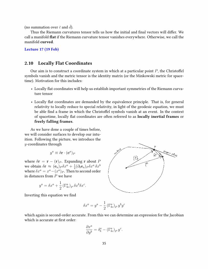
As we have done a couple of times before,we will consider surfaces to develop our intu-ition. Following the picture, we introduce they-coordinates through

ya ≡ δr · (ea)P

where δr = r − (r)P . Expanding r about Pwe obtain δr ≈ (ea)P δx

a + 12(∂bea)P δx

a δxb

where δxa = xa−(xa)P . Then to second orderin distances from P we have

ya = δxa +1

2(Γabc)P δx

bδxc.

Inverting this equation we nd

δxa = ya − 1

2(Γabc)P y

byc

which again is second-order accurate. From this we can determine an expression for the Jacobianwhich is accurate at rst order:

∂xa

∂yb= δab − (Γabc)P y

c.

35

We use this to nd the metric in the y-coordinate system gab (we will use tildes to denote quantitiesin the y-coordinate system) as

gab =∂xc

∂ya∂xd

∂ybgcd ≈ gab − (Γabc)Py

c − (Γbac)Pyc = gab − (∂cgab)Py

c

which is accurate at rst order. In the second equality, we have used the denition of the Christof-fel symbols. From this we nd(

∂gab∂yc

)P

=

(∂xd

∂yc∂gab∂xd

)P

− (∂cgab)P = 0.

Note that at point P , ∂xd

∂yc= δdc . From the denition of the Christoel symbols, from this we

conclude that all Christoel symbols in the y-coordinate system will also vanish at P :(Γabc

)P

= 0.

Lecture 18 (22 Feb)

We can go further. Let’s introduce a z-coordinate system which is related to the y-coordinatesystem as

ya = Sabzb.

In this, we take the components of S to be constants. We will use double-tildes to denote quan-tities in the z-coordinate system. For the metric tensor,

˜gab = ScaSdbgcd.

We wish to choose S such that ˜g becomes the identity matrix. Let’s proceed by writing ma-trix equations. Since g is a symmetric metric, we can diagonalise it with an orthogonal matrix:OT gO = DwhereD is a diagonal matrix composed of the eigenvalues of g. For Riemannian man-ifolds, g will have all positive eigenvalues (while for spacetime it will have one positive and threenegative). Taking all positive eigenvalues, we will have D−1/2OT gOD−1/2 = 1. We thus chooseS = OD−1/2. Through the transformation rule for the Christoel symbols (practice problems),we see that the Christoel symbols will also vanish in the z-coordinate system.

In summary (dropping tildes and going back to xa for coordinates), for a manifold with pos-itive denite metric, we can nd a coordinate system which is at about a point P in the sensethat

gab ≈ 1ab +1

2(∂c∂dgab)P δx

cδxd

and

(Γabc)P = 0.

36

Very similar arguments can be given for spacetime. Here a locally at coordinate system will give

gµν ≈ ηµν +1

2(∂σ∂ρgµν)P δx

σδxρ

and

(Γµνσ)P = 0.

2.10.1 Symmetries of the Riemann Tensor

In locally at coordinates, the Riemann curvature tensor is

(Rabcd)P = (∂cΓ

abd − ∂dΓacb)P .

Recalling that rst-order derivatives of the metric tensor vanish at point P , we nd (check),

(Rabcd)P =1

2(∂b∂cgad + ∂a∂dgbc − ∂b∂dgac − ∂a∂cgbd)P .

In comparison with the general expression of the curvature tensor in terms of the metric tensor,the above expression is vastly simplied. From this we can directly verify the symmetries of theRiemann curvature tensor written earlier at point P in our locally at coordinate system.

However, since Rabcd is a tensor, it is enough to establish the symmetries Eq. 31 in a single

coordinate system. For instance, we have for locally at coordinates, (Rabcd)P = −(Rbacd)P . Wecan use Jacobian matrices to transform to another coordinate system (which need not be locallyat) and nd (Ra′b′c′d′)P = −(Rb′a′c′d′)P . The nal point to note is that P is arbitrary.

2.11 Tensors Derived From the Riemann Curvature Tensor and the Ein-stein Field Equation

For later use, we will now introduce tensors which follow from the Riemann curvature tensor.The Ricci tensor Rab is dened as

Rab = Rcacb.

From the symmetries of the Riemann tensor (how?), we see that Rab is symmetric: Rab = Rba.The Ricci scalar R follows from the Ricci tensor as

R = Raa = gabRba.

Finally, the Einstein tensor Gab is dened as

Gab = Rab −1

2gabR.

37

The Einstein eld equations are

Gµν =8πG

c4Tµν

where Tµν is the energy-momentum tensor which we will look at soon. For a particular energymomentum tensor, we solve the Einstein eld equations to determine the metric. The analogywith Newtonian gravity is: given a mass distribution ρ(r), we solve Poisson’s equation to de-termine the gravitational potential. In due course we will verify that Einstein’s eld equationsreduce to Poisson’s equation in the non-relativistic limit. Then with this metric, we can solve thegeodesic equation to determine the trajectory of a particle in this eld. J. A. Wheeler succinctlydescribed this process as “Spacetime tells matter how to move; matter tells spacetime how tocurve.”

2.12 The Bianchi Identity and the Contracted Bianchi IdentityWe will need a couple more relations for the Riemann curvature tensor. The Riemann curva-

ture tensor satises the Bianchi identity:

∇eRabcd +∇dR

abec +∇cR

abde = 0. (32)

Like the symmetries of Riemann tensor established earlier, the Bianchi identity is easiest to estab-lish by using locally at coordinates. For such a coordinate system (since the Christoel symbolsvanish)

(∇eRabcd)P = (∂eR

abcd)P = (∂e∂cΓ

abd − ∂e∂dΓacb)P .

From this, we can directly verify Eq. 32.

Lecture 19 (23 Feb)

From the Bianchi identity, we can derive the contracted Bianchi identity which reads

∇aGab = 0. (33)

First, contract a and c in the Bianchi identity to nd

∇eRbd −∇dRbe +∇aRabde = 0.

For the second term, we have used Eq. 31: ∇dRabea = ∇d(g

afRfbea) = −∇d(gafRfbae) =

−∇dRabae = −∇dRbe. Since ∇cg

ab = 0, for a tensor eld Xa we have gac∇bXa = ∇bXc.

With this in mind, we can “raise indices behind the covariant derivative operator”. Raise b andcontract with d to nd

∇eR−∇bRbe +∇aR

abbe = 0.

38

Let’s work on the last term on the left-hand side:

∇aRabbe = gafgbh∇aRfhbe = −gafgbh∇aRhfbe

= −gaf∇aRbfbe = −gaf∇aRfe = −∇aR

ae.

So the above becomes

∇eR− 2∇bRbe = 0.

Relabelling indices,

∇a(Rab −

1

2δabR) = 0.

Finally, raising b we obtain ∇a(Rab − 1

2gabR) = 0 which is Eq. 33.

2.13 Relativistic Fluids and the Energy-Momentum TensorThe remaining piece of Einstein’s eld equation which we need to address is the energy-

momentum tensor T µν . For most situations in this course, we will take the energy-momentumtensor for a perfect uid which reads

T µν = (ρ+ p/c2)uµuν − pgµν .

In our discussion of special relativity, we introduced the four-velocity of a particle. We nowgeneralise uµ to a vector eld so that (uµ)P describes the average four-velocity of particles at pointP in spacetime. We take ρ to be the proper density (mass density measured in a momentarilyco-moving frame) of the matter. The pressure, which also can depend on position is p. Both ρand p are scalars.

We take the equations of motion of the relativistic uid to be given by

∇µTµν = 0.

Note the consistency between this and the eld equations as a result of the contracted Bianchiidentity. We will follow our usual practice of showing that these equations of motion reduce tosomething sensible in the non-relativistic limit. We will now work on writing these equations ofmotion in a more intuitive way.

First some useful relations. Since uµuµ = c2, we have that uν∇µuν = uν∇µuν = 0. For our

perfect uid we also have T µνuν = ρc2uµ. Multiply our equations of motion by uν (and sum asusual over ν):

0 = uν∇µTµν = ∇µ(T µνuν)− T µν∇µuν = ∇µ(c2ρuµ) + p∇µu

µ.

So

∇µ(ρuµ) +p

c2∇µu

µ = 0. (34)

39

To obtain our other uid equation, we use the projection tensor

P µν = δµν −

1

c2uµuν .

Note that P µν uµ = 0 and P µ

σ Pσν = P µ

ν . This enables us to look at components of the uid equationorthogonal to the four-velocity eld. With this,

0 = P σν ∇µT

µν = P σν

((ρ+ p/c2)uµ∇µu

ν − gµν∂µp)

= (ρ+ p/c2)uµ∇µuσ − ∂µp(gµσ − uµuσ/c2).

Relabelling indices,

(ρ+ p/c2)uµ∇µuν = ∂µp(g

µν − uµuν/c2). (35)

Eqns. 34, 35 give a more explicit description of the equations of motion of relativistic uids.They reduce to the continuity and Euler equations from uid mechanics11 in the non-relativisticlimit. In particular, we consider the limit where ρ p/c2, gµν = ηµν , and uµ = (c,v) where v isthe velocity eld of the uid. In this limit, Eq. 34 becomes (exercise)

∂tρ = −−→∇ · (ρv)

which is the continuity equation. The µ = 1, 2, 3 components of Eq. 35 become (exercise)

ρ(∂tv + (v ·−→∇)v) = −

−→∇p

which is the Euler equation.

Lecture 20 (26 Feb)

Example: Dust in Special Relativity. A relativistic uid in the absence of pressure is re-ferred to as dust. In this example we will look at dust in special relativity where gµν = ηµνand hence ∇µ = ∂µ. Using uµ = γ(c,v) and writing out the spatial, temporal, and mixedcomponents of the energy-momentum tensor impels us to introduce ρ = γ2ρ. We thenhave

T 00 = ρc2

T 0i = T i0 = ρcvi

T ij = ρvivj

where v is the coordinate velocity (or three-velocity) eld. Note that since vi is not a tensorwe have the unusual placement of indices. ρ is in fact the frame-dependent density ofthe uid. The combined eect of length contraction and relativistic enhancement of mass

11A description of classical ideal uids is outside the scope of this course. If you haven’t seen these equations, Irecommend The Feynman Lectures on Physics for an accessible introduction.

40

provides the factor of γ2. It can be veried that the equations of motion ∂µT µν = 0 can bewritten, without approximation, as (exercise)

∂tρ = −−→∇ · (ρv)

and

∂tv + (v ·−→∇)v = 0.

Unlike Eqns. 34 and 35, the above are not tensor equations. These equations provide per-haps the clearest connection with classical ideal uids.

Lecture 21 (29 Feb)

2.14 Weak Field Limit of the Einstein Field EquationsWe need to show that the Einstein Field Equations reduce to Poisson’s equation in the non-

relativistic limit. To do this, it is helpful to write the eld equations in an alternative way. Letκ = 8πG

c4. Then the eld equations are

Rµν − 1

2gµνR = κT µν .

Lowering ν and contracting with µ and noting that gµµ = δµµ = 4, we have

R = −κT

where T ≡ T µµ. Putting this back into the eld equations we nd

Rµν = κ(T µν − 1

2gµνT ) (36)

or, lowering indices,

Rµν = κ(Tµν −1

2gµνT ) (37)

which is an alternative way of writing the eld equations. As a special case when Tµν = 0 thisreduces to

Rµν = 0

which are the vacuum eld equations.We consider the limiting case of small velocities v/c 1. The metric is taken to be time

independent and nearly at: gµν = ηµν +hµν where |hµν | 1. We further require that p/c2 ρ.

41

With these requirements, the 00 component of the energy momentum tensor will be dominant.We have T00 ≈ T 00 ≈ ρc2 and T = T µµ = (ρ+ p/c2)c2 − 4p ≈ ρc2. With this, we nd

R00 = κ(T00 −1

2g00T ) ≈ κ

2ρc2. (38)

Now let’s consider the 00 component of the Ricci tensor in this limit. To rst order in hµν ,

Rµνρσ = ∂ρΓ

µνσ − ∂σΓµνρ

and so to this order,

R00 = Rµ0µ0 = ∂µΓµ00 − ∂0Γµ0µ = ∂µΓµ00

(recall we are taking the metric to be time-independent). Recalling some results from 2.8.2, wehave to rst order in hµν

R00 = ∂µΓµ00 = −1

2ηµν∂µ∂νh00 =

1

2

−→∇2h00 =

1

c2

−→∇2Φ.

Inserting this into Eq. 38 we nd Poisson’s equation:−→∇2Φ = 4πGρ.

3 General Relativity Applied

3.1 The Schwarzschild GeometryIt is now time to put the theory of general relativity uncovered during the last chapter to

work.We seek to nd the spacetime metric corresponding to a spherically-symmetric massive body

of total mass M . We will solve the vacuum eld equations

Rµν = 0

which are valid outside of the massive body’s interior. We take the metric to be sphericallysymmetric, time-independent, and asymptotically at. The following ansatz satises these threeconditions:

(ds)2 = c2e2A(r)(dt)2 − e2B(r)(dr)2 − r2(dθ)2 − r2 sin2(θ)(dφ)2.

where we require A,B → 0 as r → ∞ so that the metric reduces to the Minkowski metric atlarge distances from the body.12 From this, we can compute the Ricci tensor13. One nds the

12 Actually, one can arrive at this metric by starting with a general spherically symmetric metric and applyingcertain variable changes.

13Read o the metric from (ds)2. From the metric, compute the Christoel symbols. From the Christoel symbolscompute the Riemann tensor. From the Riemann tensor, compute the Ricci tensor. This is a straightforward butcomputationally intensive task and is perhaps best left to a symbolic mathematics package likeMaple orMathematica.

42

non-vanishing components are

R00 = e2(A−B)(A′2 +2

rA′ − A′B′ + A′′)

R11 = −A′2 +2

rB′ + A′B′ − A′′

R22 = e−2B(−1 + e2B − rA′ + rB′)

R33 = sin2(θ)R22.

In the above, primes denote derivatives with respect to r. Combining the equations for R00 andR11 gives A′ +B′ = 0. Using our boundary condition then gives A+B = 0. Inserting A = −Binto the equation for R22 gives

2rA′ + 1 = e−2A.

With the substitution A(r) = 12

log(ψ(r)), this equation becomes rψ′ + ψ = 1 which has thesolution ψ(r) = 1 + k

rwhere k is a constant. With this we have

(ds)2 = c2(1 +k

r)(dt)2 − 1

1 + kr

(dr)2 − r2(dθ)2 − r2 sin2(θ)(dφ)2.

How do we determine k? We require that the metric reduces to the correct weak-eld limit for agravitational potential Φ(r) = −GM

r. Using results from the previous chapter, we require

g00 = 1 +k

r= 1 + h00 = 1 +

2

c2Φ(r).

We then nd k = −2MG/c2. With this value for k, we have found the Schwarzschild metric.

Lecture 22 (1 Mar)

3.2 Classical Kepler MotionBefore considering motion under the Schwarzschild metric, we will rst, for comparison and

to set some notation, consider the Newtonian motion of a particle under a gravitational potentialΦ(r) = −MG

r. We take the mass of the particle m to be much smaller than M so that we can

avoid working with “reduced masses”. That is, we can take the position of the larger mass M tobe xed in space. Newton’s second law reads

d2r

dt2= −−→∇Φ = −MG

r2r.

The angular momentum L = r×mdrdt

is conserved:

dL

dt=dr

dt×mdr

dt+ r×

(−mGr2

r

)= 0.

43

SinceL is conserved and r·L = 0, the motion will be conned to a plane. We use polar coordinates(r, φ) for this plane.

From classical mechanics, drdt

= φφ and dφdt

= −φr. Using this,

d2r

dt2=

d2

dt2(rr) = (r − rφ2)r +

1

r

d

dt(r2φ)φ =

−MG

r2r.

So

r − rφ2 = −MG

r2, and

d

dt(r2φ) = 0. (39)

It is useful to introduce u = 1/r and regard r as a function of φ (compare with the compu-tation of geodesics on the unit sphere). Let h = r2φ which is a constant of motion by the aboveequations. Then

dr

dt=dr

du

du

dφφ = −hdu

dφ

and

d2r

dt2= −hd

2u

dφ2φ = −h2u2 d

2u

dφ2

Inserting this into Eq. 39 we nd

d2u

dφ2+ u =

GM

h2

which is the Binet equation. It has the solution

u(φ) =GM

h2(1 + e cos(φ− φ0)).

Where φ0 and e are constants. e is called the eccentricity. We obtain circular, elliptic, parabolic,and hyperbolic motion for e = 0, 0 < |e| < 1, |e| = 1, and |e| > 1 respectively. For instance, forφ0 = 0 and |e| 6= 1, we can write this solution as

(1− e2)

(x+

Re

1− e2

)2

+ y2 =R2

1− e2

where R = h2

GM.

3.3 Precision of the PerihelionWe will now consider the analogous problem in general relativity, of a massive particle in

orbit.

44

It is convention to dene m = MGc2

. This quantity has units of length. With this, theSchwarzschild line element is

(ds)2 =

(1− 2m

r

)c2(dt)2 −

(1− 2m

r

)−1

(dr)2 − r2(dΩ)2

where (dΩ)2 = sin2(θ)(dφ)2 + (dθ)2. This is related to the proper time dierential in the usualway for massive particles: (ds)2 = c2(dτ)2. Since τ is an ane parameter, the geodesic equationwill be given by the Euler-Lagrange equations of K = 1

2gµν x

µxν .Let’s rst search for conserved quantities. Since the metric does not explicitly depend on φ

or t, the corresponding Euler-Lagrange equations gives the conserved quantities

k =

(1− 2m

r

)t

h = r2 sin2(θ)φ.

Additionally, K = 12

(dsdτ

)2= 1

2c2 itself is conserved. As in the previous section, we consider

planar motion and set θ = π/2. Inserting our conserved quantities into K and reintroducingu = 1/r (see previous section), we nd

c2k2 − h2

(du

dφ

)2

= (c2 + h2u2)(1− 2mu).

Next we dierentiate the above with respect to φ to nd

d2u

dφ2+ u =

c2m

h2+ 3mu2.

This is the relativistic Binet equation. The dierence between this and the Binet equation fromthe previous section is the last term on the right-hand side, which makes the current equation anon-linear ode. Using the mass of the sun for M , we nd m = MG/c2 ≈ 1500 m. This is wellwithin the radius of the sun. Therefore, for typical planetary motion, um = m/r will be a smallnumber and the last term on the right-hand side of the relativistic Binet equation can be viewedas a small correction. Its role in solar system motion is typically small but sometimes measurable.This term will be largest for planets close to the sun.

Lecture 23 (4 Mar)

In the following we will consider nearly circular motion and write u = u0 + δu where u0 is aconstant and δu u0. Putting this into Binet’s equation, we have to zeroth and rst order in δu,

u0 =c2m

h2+ 3mu2

0

d2δu

dφ2+ δu = 6mu0δu.

45

Solving the second equation, δu = A cos(√

1− 6mu0(φ − φ0)) where A and φ0 are constants.So,

u = u0 + δu = u0[1 + e cos(√

1− 6mu0φ)]

where we have put φ0 = 0 for convenience.The point of closest approach to the sun is referred to as the perihelion. Unlike Kepler

motion, the above predicts that the perihelion will precess. The observation of this eect for theplanet Mercury was one of the earliest observational tests of general relativity.

Let’s take e > 0. Then the values ofφ corresponding to perihelia areφn = 2πn/√

1− 6mu0 ≈2πn(1 + 3mu0) for integer n. From this we see that after every orbit, the perihelion will advanceby

∆φ = 6πmu0.

Putting in approximate numbers for Mercury (89 days per orbit, 1/u0 ≈ 5.8 × 1010 m), we ndthat after a century its perihelion will advance by 42 arcseconds (602 arcseconds = 1). Theobservational value is 43.1± .5 arcseconds.14

3.4 General Orbits in the Schwarzschild GeometryWe will now broaden our discussion to include the motion of photons. From our discussion

of photons in special relativity, we have the result (ds)2 = ηµνdxµdxν = (c2− v2)(dt)2 = 0 from

the rst postulate. This result continues to hold in general relativity where (ds)2 = gµνdxµdxν .

We conclude this by appealing to locally at coordinates. That is, we can nd a coordinate systemin which gµν locally reduces to ηµν . By the equivalence principle, we can nd a frame in whichspecial relativity locally holds. In this frame (ds)2 = 0. However, since (ds)2 is a scalar quantity,this must hold in all frames. Proper time is ill dened for photons. We therefore need to choosea dierent ane parameter, which we call w, with which to describe their motion.

In order to not produce fairly similar derivations for light and massive particles we write thefollowing:

gµν xµxν = αc2

where α = 0 and xµ = dxµ/dw for light while α = 1 and xµ = dxµ/dτ for massive particles.As before, for geodesic motion, we have the conserved quantities h = r2φ and k = (1− 2m/r)twhere we are still restricting to planar motion θ = π/2. Inserting these into the above, we obtain

1

2r2 + V (r) = E

14Actually, the perihelion of Mercury will also precess according to Newton’s laws. This is the result of grav-itational elds from sources other than those of Mercury and the sun. More precisely, the amount of additionaladvancement (not accounted for by Newton’s laws) is (43.1± .5) arcseconds per century.

46

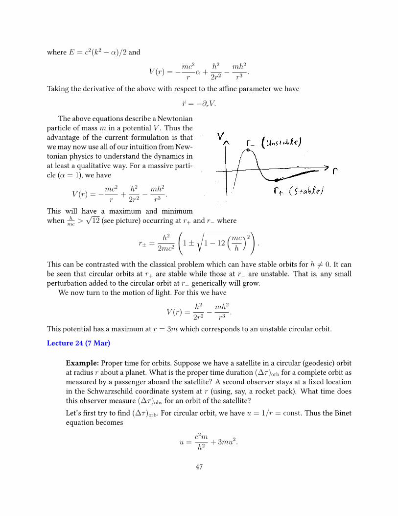
where E = c2(k2 − α)/2 and

V (r) = −mc2

rα +

h2

2r2− mh2

r3.

Taking the derivative of the above with respect to the ane parameter we have

r = −∂rV.

97

91

98

99 100

The above equations describe a Newtonianparticle of mass m in a potential V . Thus theadvantage of the current formulation is thatwe may now use all of our intuition from New-tonian physics to understand the dynamics inat least a qualitative way. For a massive parti-cle (α = 1), we have

V (r) = −mc2

r+

h2

2r2− mh2

r3.

This will have a maximum and minimumwhen h

mc>√

12 (see picture) occurring at r+ and r− where

r± =h2

2mc2

(1±

√1− 12

(mch

)2).

This can be contrasted with the classical problem which can have stable orbits for h 6= 0. It canbe seen that circular orbits at r+ are stable while those at r− are unstable. That is, any smallperturbation added to the circular orbit at r− generically will grow.

We now turn to the motion of light. For this we have

V (r) =h2

2r2− mh2

r3.

This potential has a maximum at r = 3m which corresponds to an unstable circular orbit.

Lecture 24 (7 Mar)

Example: Proper time for orbits. Suppose we have a satellite in a circular (geodesic) orbitat radius r about a planet. What is the proper time duration (∆τ)orb for a complete orbit asmeasured by a passenger aboard the satellite? A second observer stays at a xed locationin the Schwarzschild coordinate system at r (using, say, a rocket pack). What time doesthis observer measure (∆τ)obs for an orbit of the satellite?Let’s rst try to nd (∆τ)orb. For circular orbit, we have u = 1/r = const. Thus the Binetequation becomes

u =c2m

h2+ 3mu2.

47

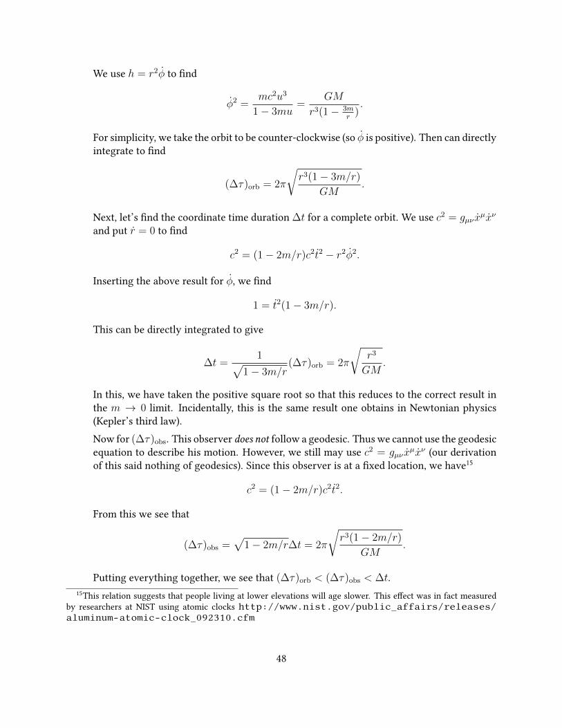
We use h = r2φ to nd

φ2 =mc2u3

1− 3mu=

GM

r3(1− 3mr

).

For simplicity, we take the orbit to be counter-clockwise (so φ is positive). Then can directlyintegrate to nd

(∆τ)orb = 2π

√r3(1− 3m/r)

GM.

Next, let’s nd the coordinate time duration ∆t for a complete orbit. We use c2 = gµν xµxν

and put r = 0 to nd

c2 = (1− 2m/r)c2t2 − r2φ2.

Inserting the above result for φ, we nd

1 = t2(1− 3m/r).

This can be directly integrated to give

∆t =1√

1− 3m/r(∆τ)orb = 2π

√r3

GM.

In this, we have taken the positive square root so that this reduces to the correct result inthe m → 0 limit. Incidentally, this is the same result one obtains in Newtonian physics(Kepler’s third law).Now for (∆τ)obs. This observer does not follow a geodesic. Thus we cannot use the geodesicequation to describe his motion. However, we still may use c2 = gµν x

µxν (our derivationof this said nothing of geodesics). Since this observer is at a xed location, we have15

c2 = (1− 2m/r)c2t2.

From this we see that

(∆τ)obs =√

1− 2m/r∆t = 2π

√r3(1− 2m/r)

GM.

Putting everything together, we see that (∆τ)orb < (∆τ)obs < ∆t.15This relation suggests that people living at lower elevations will age slower. This eect was in fact measured

by researchers at NIST using atomic clocks http://www.nist.gov/public_affairs/releases/aluminum-atomic-clock_092310.cfm

48

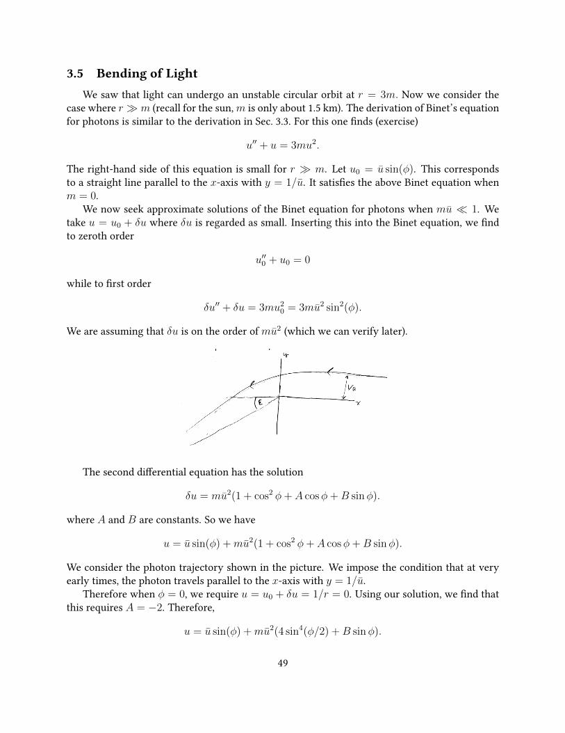
3.5 Bending of LightWe saw that light can undergo an unstable circular orbit at r = 3m. Now we consider the

case where r m (recall for the sun,m is only about 1.5 km). The derivation of Binet’s equationfor photons is similar to the derivation in Sec. 3.3. For this one nds (exercise)

u′′ + u = 3mu2.

The right-hand side of this equation is small for r m. Let u0 = u sin(φ). This correspondsto a straight line parallel to the x-axis with y = 1/u. It satises the above Binet equation whenm = 0.

We now seek approximate solutions of the Binet equation for photons when mu 1. Wetake u = u0 + δu where δu is regarded as small. Inserting this into the Binet equation, we ndto zeroth order

u′′0 + u0 = 0

while to rst order

δu′′ + δu = 3mu20 = 3mu2 sin2(φ).

We are assuming that δu is on the order of mu2 (which we can verify later).

Lecture 22 (3/3/14)

101 102

103 104

The second dierential equation has the solution

δu = mu2(1 + cos2 φ+ A cosφ+B sinφ).

where A and B are constants. So we have

u = u sin(φ) +mu2(1 + cos2 φ+ A cosφ+B sinφ).

We consider the photon trajectory shown in the picture. We impose the condition that at veryearly times, the photon travels parallel to the x-axis with y = 1/u.

Therefore when φ = 0, we require u = u0 + δu = 1/r = 0. Using our solution, we nd thatthis requires A = −2. Therefore,

u = u sin(φ) +mu2(4 sin4(φ/2) +B sinφ).

49

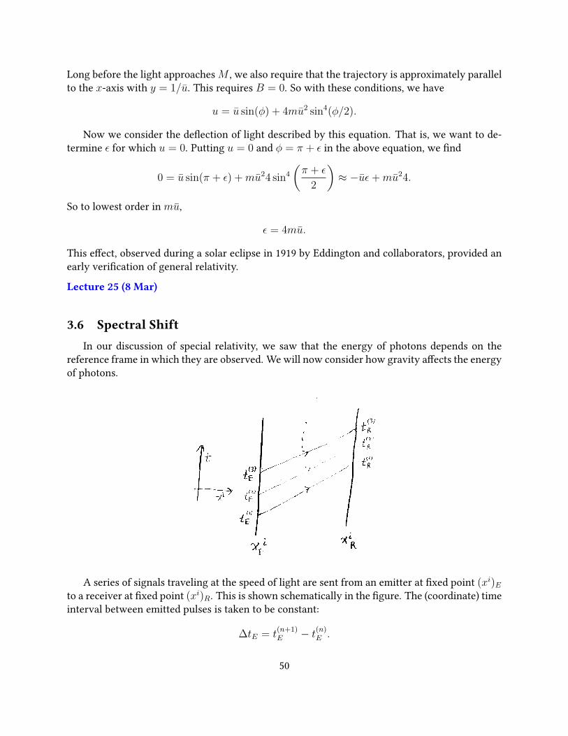
Long before the light approaches M , we also require that the trajectory is approximately parallelto the x-axis with y = 1/u. This requires B = 0. So with these conditions, we have

u = u sin(φ) + 4mu2 sin4(φ/2).

Now we consider the deection of light described by this equation. That is, we want to de-termine ε for which u = 0. Putting u = 0 and φ = π + ε in the above equation, we nd

0 = u sin(π + ε) +mu24 sin4

(π + ε

2

)≈ −uε+mu24.

So to lowest order in mu,

ε = 4mu.

This eect, observed during a solar eclipse in 1919 by Eddington and collaborators, provided anearly verication of general relativity.

Lecture 25 (8 Mar)

3.6 Spectral ShiftIn our discussion of special relativity, we saw that the energy of photons depends on the

reference frame in which they are observed. We will now consider how gravity aects the energyof photons.

Lecture 22 (3/3/14)

101 102

103 104

A series of signals traveling at the speed of light are sent from an emitter at xed point (xi)Eto a receiver at xed point (xi)R. This is shown schematically in the gure. The (coordinate) timeinterval between emitted pulses is taken to be constant:

∆tE = t(n+1)E − t(n)

E .

50

For light, we have

0 = (1− 2m/r)c2t2 + gijxixj

where, as before, i, j are summed only over spatial components. From this we can calculate

t(1)R − t

(1)E =

1

c

∫ xiR

xiE

√−gij(1− 2m/r)−1dxidxj.

The right-hand side of this only depends on the path through space. So

t(n)R − t

(n)E

is the same for all n. So t(n)R − t

(n)E = t

(n+1)R − t(n+1)

E . This gives

∆tE = t(n+1)E − t(n)

E = t(n+1)R − t(n)

R ≡ ∆tR.

The coordinate-time duration between pulses received is the same as the coordinate-time dura-tion between pulses emitted.

Now take two observers situated at xiE and xiR. The proper time measured by these observersis related to coordinate time as

c2(dτE)2 = (1− 2m/rE)c2(dt)2

c2(dτR)2 = (1− 2m/rR)c2(dt)2

We therefore nd

∆τR∆τE

=

√1− 2m/rR1− 2m/rE

∆tR∆tE

=

√1− 2m/rR1− 2m/rE

.

Converting to frequencies, νR = 1/∆τR, νE = 1/∆τE , we have

νRνE

=

√1− 2m/rE1− 2m/rR

. (40)

We arrived at this result by considering a series of signals travelling between between anemitter and receiver. This result holds also for the frequency (or energy) of light. For instance,we could imagine the two observers (in principle!) measuring instead durations between themaxima of the electric eld of a light wave.

We can arrive at the above result in a more elegant (but perhaps less transparent) way by usinga method introduced back in 1.9. Take an observer with four-velocity (uµ)obs and a photon withfour-velocity pµ. Suppose that the photon barely misses the observer at a particular spacetimepoint. At this event, the observer assigns energy hν = (uµ)obspµ to the photon. We establishedthis result for special relativity, but, through the equivalence principle it also holds in generalrelativity. Note for our Schwarzschild coordinate system, uµ = (ct, r, θ, φ).

51

For our current problem, the two observers will have four-velocities

(uµ)E = (ct, 0, 0, 0) =

(c√

1− 2m/rE, 0, 0, 0

)

(uµ)R =

(c√

1− 2m/rR, 0, 0, 0

).

For the light, since dxµ

dwis parallel to pµ, we can choose the ane parameter w such that

pµ = dxµ

dw. We take the photon to be moving radially. Using k = (1 − 2m/r)t, and taking the

photon to travel radially outward (r > 0), we have have

pµ =

(kc

1− 2m/r, kc, 0, 0

)and

pµ =

(kc,− kc

1− 2m/r, 0, 0

).

To nd pµ we have, as usual, used pµ = gµνpν .

Now we can directly evaluate the energies of the light as measured by observers at the emitterand receiver:

hνE = (uµ)Rpµ =kc2√

1− 2m/rE

hνR = (uµ)Rpµ =kc2√

1− 2m/rR.

Dividing these results, we arrive at the spectral shift formula 40.

3.7 The Pound-Rebka ExperimentWe will now consider an example which nicely combines the Doppler shift (which we saw in

special relativity) with the gravitational spectral shift. As shown in the gure, photons are emittedand travel radially inward to a receiver. Through the previous analysis, the photons will becomemore energetic, or blue shifted, as they “fall” under earth’s gravitational eld (we take M for thisexample to be the mass of the earth). On the other hand, when the emitter is moving radiallyoutward with velocity v = drE

dt> 0, we expect, through the Doppler eect, that this will decrease,

or red shift, the energy of the light. We ask: for which v will the energy of the emitted andreceived photons (as determined by observers situated at the emitter and receiver) be the same?This result is relevant for the Pound-Rebka experiment.16 In contrast to the other “classical” tests

16 Pound, R. V.; Rebka Jr. G. A. (November 1, 1959). "Gravitational Red-Shift in Nuclear Resonance". PhysicalReview Letters 3 (9): 439

52

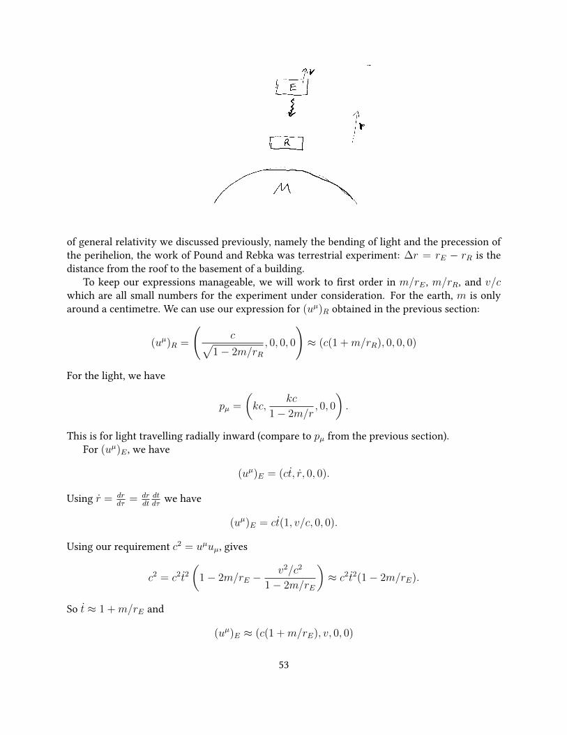
105

Lecture 23 (4/3/14)

106

107 108

of general relativity we discussed previously, namely the bending of light and the precession ofthe perihelion, the work of Pound and Rebka was terrestrial experiment: ∆r = rE − rR is thedistance from the roof to the basement of a building.

To keep our expressions manageable, we will work to rst order in m/rE , m/rR, and v/cwhich are all small numbers for the experiment under consideration. For the earth, m is onlyaround a centimetre. We can use our expression for (uµ)R obtained in the previous section:

(uµ)R =

(c√

1− 2m/rR, 0, 0, 0

)≈ (c(1 +m/rR), 0, 0, 0)

For the light, we have

pµ =

(kc,

kc

1− 2m/r, 0, 0

).

This is for light travelling radially inward (compare to pµ from the previous section).For (uµ)E , we have

(uµ)E = (ct, r, 0, 0).

Using r = drdτ

= drdt

dtdτ

we have

(uµ)E = ct(1, v/c, 0, 0).

Using our requirement c2 = uµuµ, gives

c2 = c2t2(

1− 2m/rE −v2/c2

1− 2m/rE

)≈ c2t2(1− 2m/rE).

So t ≈ 1 +m/rE and

(uµ)E ≈ (c(1 +m/rE), v, 0, 0)

53

Now we these expressions for the four-vectors, we obtain

hνE = kc2(1 +m/rE + v/c)

hνR = kc2(1 +m/rR).

The energy of the emitted and received photons will be the same when

v

c=m

rR− m

rE≈ m∆r

R2

where R is the radius of the earth. Using g = GMR2 ≈ 10 m/s2, we can write this as

v =g∆r

c.

Lecture 26 (11 Mar)

3.8 Black Holes3.8.1 Gravitational Collapse

We have been mostly concentrating on examples where general relativity provides small cor-rections to classical dynamics. We will now turn our attention to black holes where the role ofgeneral relativity is more profound.

In our derivation of the Schwarzschild metric, we concentrated on regions outside a massivebody’s interior where T µν = 0. Though we will not perform the calculation, one can solveEinstein’s equations

Gµν = κT µν

using a perfect uid for T µν for the interior regions of a spherically-symmetric star. Taking auniform density of the star: ρ = const (though this approximation is not entirely physicallysensible) one nds an interesting result: if the radius of the star is less than 9

4m, then the pressure

will diverge somewhere in the interior of the star. This signies an instability: gravitationalcollapse.

Black holes are expected to form after very massive stars collapse. In this course, we willonly consider Schwarzschild black holes, which are black holes with no angular momentum orcharge.

3.8.2 Radial free fall of a massive particle into a black hole

54

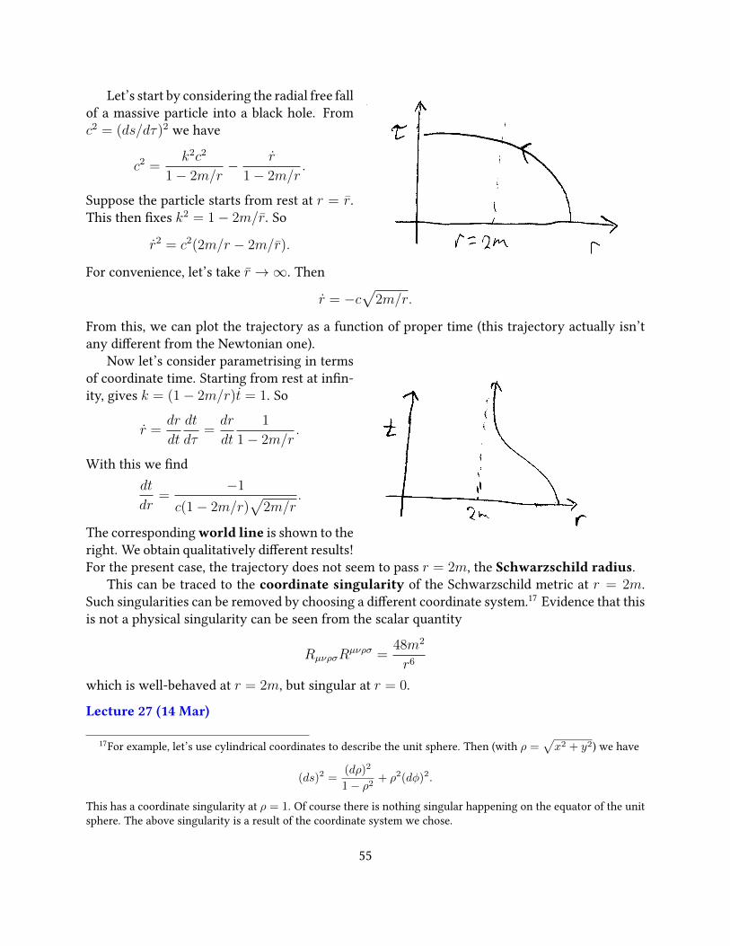
117 118

Lecture 26 (11/3/14)

119 120

Let’s start by considering the radial free fallof a massive particle into a black hole. Fromc2 = (ds/dτ)2 we have

c2 =k2c2

1− 2m/r− r

1− 2m/r.

Suppose the particle starts from rest at r = r.This then xes k2 = 1− 2m/r. So

r2 = c2(2m/r − 2m/r).

For convenience, let’s take r →∞. Then

r = −c√

2m/r.

From this, we can plot the trajectory as a function of proper time (this trajectory actually isn’tany dierent from the Newtonian one).

117 118

Lecture 26 (11/3/14)

119 120

Now let’s consider parametrising in termsof coordinate time. Starting from rest at inn-ity, gives k = (1− 2m/r)t = 1. So

r =dr

dt

dt

dτ=dr

dt

1

1− 2m/r.

With this we nddt

dr=

−1

c(1− 2m/r)√

2m/r.

The corresponding world line is shown to theright. We obtain qualitatively dierent results!For the present case, the trajectory does not seem to pass r = 2m, the Schwarzschild radius.

This can be traced to the coordinate singularity of the Schwarzschild metric at r = 2m.Such singularities can be removed by choosing a dierent coordinate system.17 Evidence that thisis not a physical singularity can be seen from the scalar quantity

RµνρσRµνρσ =

48m2

r6

which is well-behaved at r = 2m, but singular at r = 0.

Lecture 27 (14 Mar)

17For example, let’s use cylindrical coordinates to describe the unit sphere. Then (with ρ =√x2 + y2) we have

(ds)2 =(dρ)2

1− ρ2+ ρ2(dφ)2.

This has a coordinate singularity at ρ = 1. Of course there is nothing singular happening on the equator of the unitsphere. The above singularity is a result of the coordinate system we chose.

55

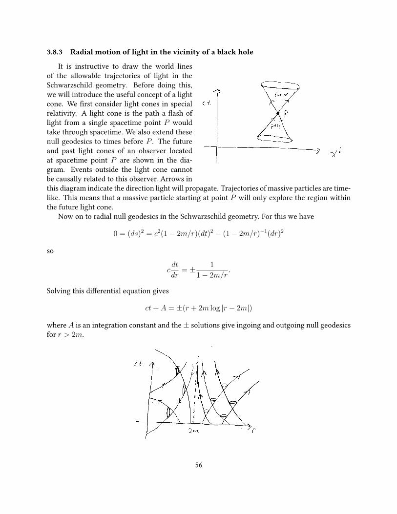
3.8.3 Radial motion of light in the vicinity of a black hole

It is instructive to draw the world linesof the allowable trajectories of light in theSchwarzschild geometry. Before doing this,we will introduce the useful concept of a lightcone. We rst consider light cones in specialrelativity. A light cone is the path a ash oflight from a single spacetime point P wouldtake through spacetime. We also extend thesenull geodesics to times before P . The futureand past light cones of an observer locatedat spacetime point P are shown in the dia-gram. Events outside the light cone cannotbe causally related to this observer. Arrows inthis diagram indicate the direction light will propagate. Trajectories of massive particles are time-like. This means that a massive particle starting at point P will only explore the region withinthe future light cone.

Now on to radial null geodesics in the Schwarzschild geometry. For this we have

0 = (ds)2 = c2(1− 2m/r)(dt)2 − (1− 2m/r)−1(dr)2

so

cdt

dr= ± 1

1− 2m/r.

Solving this dierential equation gives

ct+ A = ±(r + 2m log |r − 2m|)

where A is an integration constant and the± solutions give ingoing and outgoing null geodesicsfor r > 2m.

117 118

Lecture 26 (11/3/14)

119 120

56

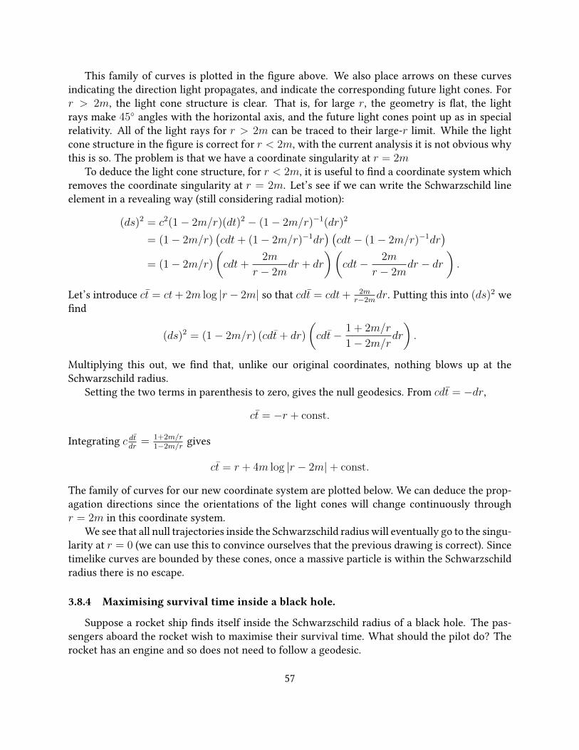
This family of curves is plotted in the gure above. We also place arrows on these curvesindicating the direction light propagates, and indicate the corresponding future light cones. Forr > 2m, the light cone structure is clear. That is, for large r, the geometry is at, the lightrays make 45 angles with the horizontal axis, and the future light cones point up as in specialrelativity. All of the light rays for r > 2m can be traced to their large-r limit. While the lightcone structure in the gure is correct for r < 2m, with the current analysis it is not obvious whythis is so. The problem is that we have a coordinate singularity at r = 2m

To deduce the light cone structure, for r < 2m, it is useful to nd a coordinate system whichremoves the coordinate singularity at r = 2m. Let’s see if we can write the Schwarzschild lineelement in a revealing way (still considering radial motion):

(ds)2 = c2(1− 2m/r)(dt)2 − (1− 2m/r)−1(dr)2

= (1− 2m/r)(cdt+ (1− 2m/r)−1dr

) (cdt− (1− 2m/r)−1dr

)= (1− 2m/r)

(cdt+

2m

r − 2mdr + dr

)(cdt− 2m

r − 2mdr − dr

).

Let’s introduce ct = ct+ 2m log |r− 2m| so that cdt = cdt+ 2mr−2m

dr. Putting this into (ds)2 wend

(ds)2 = (1− 2m/r) (cdt+ dr)

(cdt− 1 + 2m/r

1− 2m/rdr

).

Multiplying this out, we nd that, unlike our original coordinates, nothing blows up at theSchwarzschild radius.

Setting the two terms in parenthesis to zero, gives the null geodesics. From cdt = −dr,

ct = −r + const.

Integrating c dtdr

= 1+2m/r1−2m/r

gives

ct = r + 4m log |r − 2m|+ const.

The family of curves for our new coordinate system are plotted below. We can deduce the prop-agation directions since the orientations of the light cones will change continuously throughr = 2m in this coordinate system.

We see that all null trajectories inside the Schwarzschild radius will eventually go to the singu-larity at r = 0 (we can use this to convince ourselves that the previous drawing is correct). Sincetimelike curves are bounded by these cones, once a massive particle is within the Schwarzschildradius there is no escape.

3.8.4 Maximising survival time inside a black hole.

Suppose a rocket ship nds itself inside the Schwarzschild radius of a black hole. The pas-sengers aboard the rocket wish to maximise their survival time. What should the pilot do? Therocket has an engine and so does not need to follow a geodesic.

57

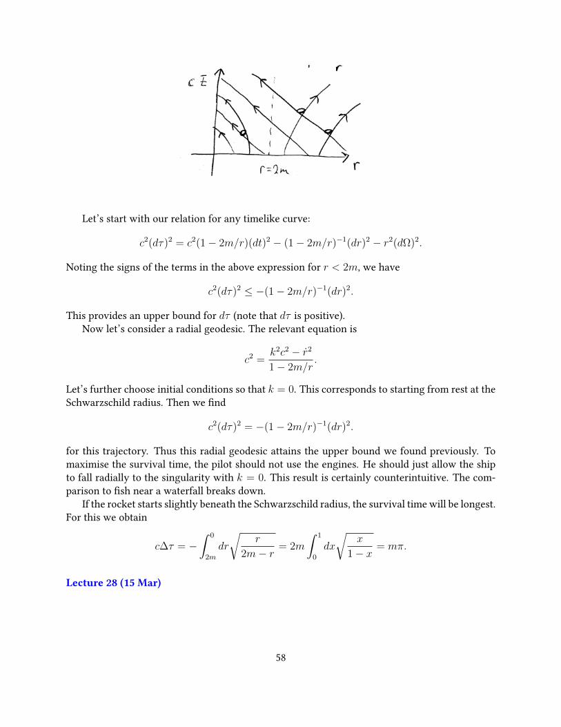
121 122

123 124

Let’s start with our relation for any timelike curve:

c2(dτ)2 = c2(1− 2m/r)(dt)2 − (1− 2m/r)−1(dr)2 − r2(dΩ)2.

Noting the signs of the terms in the above expression for r < 2m, we have

c2(dτ)2 ≤ −(1− 2m/r)−1(dr)2.

This provides an upper bound for dτ (note that dτ is positive).Now let’s consider a radial geodesic. The relevant equation is

c2 =k2c2 − r2

1− 2m/r.

Let’s further choose initial conditions so that k = 0. This corresponds to starting from rest at theSchwarzschild radius. Then we nd

c2(dτ)2 = −(1− 2m/r)−1(dr)2.

for this trajectory. Thus this radial geodesic attains the upper bound we found previously. Tomaximise the survival time, the pilot should not use the engines. He should just allow the shipto fall radially to the singularity with k = 0. This result is certainly counterintuitive. The com-parison to sh near a waterfall breaks down.

If the rocket starts slightly beneath the Schwarzschild radius, the survival time will be longest.For this we obtain

c∆τ = −∫ 0

2m

dr

√r

2m− r= 2m

∫ 1

0

dx

√x

1− x= mπ.

Lecture 28 (15 Mar)

58

3.9 Cosmology3.9.1 The Cosmological Principle

We will now move on to consider motion over much larger length scales and much longertime scales, and motivate a metric aimed at describing the geometry of the universe. In doing sowe will be guided by the cosmological principle:

• At every epoch, the universe looks the same from every spatial point except for local irreg-ularities.

The principle implies both that there are no privileged points in the universe and that there areno privileged directions about any points when viewed over suciently large length scales. Thismeans that the universe is homogeneous and isotropic. This will greatly reduce the number ofcandidate metrics we can use to describe the universe.

We take spatial coordinates which are comoving with the universe and write

(ds)2 = c2(dt)2 − (S(t))2gijdxidxj

where S is a dimensionless scale factor depending only on t. Since coordinates are comoving, tmeasures the proper time at any xed location in space. The cosmological principle requires thatthe spatial metric gij describes a maximally symmetric manifold. A maximally symmetricN -dimensional manifold is a manifold having the maximum number, N(N + 1), of independentKilling vector elds.18

3.9.2 Maximally Symmetric Three-Dimensional Manifolds

We will now deduce the spatial portion of our cosmological metric. We drop tildes and restrictto three-dimensions in what follows. The Riemann curvature tensor of a maximally symmetricmanifold can be written as

Rijkl = κ(gikgjl − gilgjk)

where κ is a constant.19 Note that this satises all of the required symmetries of the curvaturetensor. The corresponding Ricci tensor can also be seen to be constant. That is, we can work out(for three dimensions)

Rij = 2κgij, R = 6κ. (41)

Maximal symmetry of course requires spherical symmetry. A general spherically symmetricthree-dimensional metric can be written as

(ds)2 = eλ(r)(dr)2 + r2((dθ)2 + sin2 θ(dφ)2)

18The practice problems contain a question introducing Killing vector elds.19We are not showing this result, but hopefully it is plausible. See IX.6 from Zee’s book for a derivation.

59

where λ is an arbitrary function of r.From this we can compute (using, say, Mathematica)

R =2

r2e−λ(−1 + eλ + rλ′)

where primes denote derivatives with respect to r. Setting R = 6κ and solving this dierentialequation gives

e−λ(r) = 1− κr2 + A/r

where A is a constant of integration. Rab = 2κgab further requires A = 0. The resulting lineelement

(ds)2 =1

1− κr2(dr)2 + r2(dΩ)2

has Riemann curvature tensor of the form 41.To gain some intuition about these metrics, it is useful to embed the manifold in a four-

dimensional space.

κ > 0 / positive curvature / closed: Let r = 1√κ

sin(χ). Then

(ds)2 =1

κ

((dχ)2 + sin2 χ(dΩ)2

).

Introduce the new variables

w = R cos(χ)

x = R sin(χ) sin(θ) cos(φ)

y = R sin(χ) sin(θ) sin(φ)

z = R sin(χ) cos(θ)

where R = 1/√κ. Then w2 + x2 + y2 + z2 = R2 and

(ds)2 = (dw)2 + (dx)2 + (dy)2 + (dz)2.

Thus we can think of this manifold as a three-dimensional sphere embedded in four-dimensionalEuclidean space. This manifold is closed in the sense that it has nite volume.

κ = 0 / zero curvature / at: When κ = 0, the metric clearly describes three-dimensional Eu-clidean space.

κ < 0 / negative curvature / open: Let r = 1√|κ|

sinh(χ). Then

(ds)2 =1

κ

((dχ)2 + sinh2 χ(dΩ)2

).

60

Introduce the new variables

w = R cosh(χ)

x = R sinh(χ) sin(θ) cos(φ)

y = R sinh(χ) sin(θ) sin(φ)

z = R sinh(χ) cos(θ)

where R = 1/√|κ|. Then w2 − x2 + y2 + z2 = R2 and

(ds)2 = −(dw)2 + (dx)2 + (dy)2 + (dz)2.

Thus we can think of this manifold as a three-dimensional hyperboloid embedded in a at Minkowskispace with +2 signature. This manifold is open in the sense that it has innite volume.

3.9.3 The Friedmann-Robertson-Walker Metric

With these three possibilities in mind, we now return to spacetime. Things will be simpler ifwe scale the r variable. For nonzero κ, let r → r/

√|κ| while for κ = 0, we leave r unchanged.

Additionally, let R(t) = S(t)√|κ|

for non-zero κ and R(t) = S(t) when κ = 0. With this we obtainthe line element

(ds)2 = c2(dt)2 − (R(t))2

(1

1− kr2(dr)2 + r2(dΩ)2

). (42)

In this, k is either 1,0, or -1 which respectively corresponds to a closed, at, or open universe. Eq.42 denes the Friedmann-Robertson-Walker (FRW) metric.

Lecture 29 (18 Mar)

3.9.4 A Perfect Comoving Fluid

We will now ll the universe up with a perfect comoving uid with uµ = (c, 0, 0, 0) and

T µν = (ρ+ p/c2)uµuν − pgµν .

The pressure p and the proper density ρ are taken to be functions of t only. This form of theenergy-momentum tensor is again motivated by the cosmological principle. First we consider theequations of motion ∇µT

µν = 0. In Sec. 2.13 we found the following relativistic uid equations

∇µ(ρuµ) +p

c2∇µu

µ = 0 (43)

and

(ρ+ p/c2)uµ∇µuν = ∂µp(g

µν − uµuν/c2). (44)

61

Let’s plug uµ = (c, 0, 0, 0) into these equations.The right-hand side of Eq. 44 is zero. This is because p depends only on time, and g00 = 1 for

the FRW metric. For the left-hand side we consider

uµ∇µuν = c∇0u

ν = cΓν0σuσ = c2Γν00.

For the FRW metric, one can see that Γν00 = 0 for all ν and so uµ∇µuν = 0. Therefore Eq. 44 gives

no information. For Eq. 43, we need to evaluate the divergence of the four-velocity eld. We nd

∇µuµ = ∂µu

µ + Γµµνuν = Γµµ0c.

Using the denition of the Christoel symbol, we have in general (check)

Γµµν =1

2gµσ∂νgµσ.

Using the FRW metric, we nd

Γµµ0 =1

2gµσ∂0gµσ = 3

R

cR

where R = dR/dt. Thus

∇µuµ = 3R/R.

Finally, inserting this expression for the∇µuµ into Eq. 43, we nd

d

dt(ρR3) +

p

c2

d

dtR3 = 0. (45)

Thus the relativistic uid equations reduce to the relatively simple equation above for the comov-ing perfect uid.

3.9.5 Cosmological Field Equations

Now we consider the Einstein eld equations for our FRW metric with the energy-momentumtensor of the previous section. The 00 component of the Einstein tensor is computed to be

G00 = 3k + R2/c2

R2.

Noting that T00 = ρc2, G00 = 8πGc4T00 becomes

R2 + kc2 − 8π

3GρR2 = 0 (46)

which is typically called the Friedmann equation. The other components of the Einstein eldequations do not produce any additional independent equations.

The relevant equations governing the dynamics of the universe are 45, 46, and the equationof state which relates ρ to p (more on this later). With initial data, these three equations can besolved to determine the dynamics of the universe (under the assumptions of the model).

Lecture 30 (21 Mar)

62

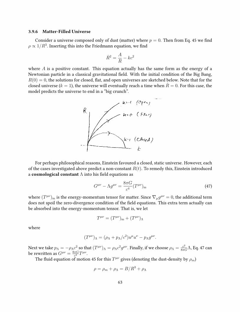
3.9.6 Matter-Filled Universe

Consider a universe composed only of dust (matter) where p = 0. Then from Eq. 45 we ndρ ∝ 1/R3. Inserting this into the Friedmann equation, we nd

R2 =A

R− kc2

where A is a positive constant. This equation actually has the same form as the energy of aNewtonian particle in a classical gravitational eld. With the initial condition of the Big Bang,R(0) = 0, the solutions for closed, at, and open universes are sketched below. Note that for theclosed universe (k = 1), the universe will eventually reach a time when R = 0. For this case, themodel predicts the universe to end in a “big crunch”.

133 134

Lecture 30 (20/3/14)

135 136

For perhaps philosophical reasons, Einstein favoured a closed, static universe. However, eachof the cases investigated above predict a non-constant R(t). To remedy this, Einstein introduceda cosmological constant Λ into his eld equations as

Gµν − Λgµν =8πG

c4(T µν)m (47)

where (T µν)m is the energy-momentum tensor for matter. Since∇µgµν = 0, the additional term

does not spoil the zero-divergence condition of the eld equations. This extra term actually canbe absorbed into the energy-momentum tensor. That is, we let

T µν = (T µν)m + (T µν)Λ

where

(T µν)Λ = (ρΛ + pΛ/c2)uµuν − pΛg

µν .

Next we take pΛ = −ρΛc2 so that (T µν)Λ = ρΛc

2gµν . Finally, if we choose ρΛ = c2

8πGΛ, Eq. 47 can

be rewritten as Gµν = 8πGc4T µν .

The uid equation of motion 45 for this T µν gives (denoting the dust-density by ρm)

ρ = ρm + ρΛ = B/R3 + ρΛ

63

where B is a positive constant. Inserting this into Friedmann equation, we nd

1

2R2 + V (R) = −1

2kc2

where

V (R) = −CR2 −D/R

(C and D are positive constants). These equations describe a Newtonian particle in the potentialV (R). Since V (R) has an extremum for which V < 0, it is possible to obtain a static universewhen k = 1. However, shortly after the development of these ideas, experimental data appearedshowing the red shift of distant stars and thus indicating that the universe is in fact expanding(R > 0) and not static.

3.9.7 Multi-component cosmological uid

More complete cosmological models allow the matter in the universe to consist of severalcomponents. We take three components: radiation, matter, and vacuum density. We write theenergy-momentum tensor, density, and pressure as a sum over components:

T µν =∑i

(T µν)i

ρ =∑i

ρi

p =∑i

pi

We further take the uid components to be non-interacting, and thus take

∇µ(T µν)i = 0

for each component. The density and pressure of each component are related by an equation ofstate:

pi = wiρic2.

For matter, vacuum density, and radiation, wi is 0, -1, and 1/3 respectively.Knowledge of the density and the scale factor R(t) of a particular uid component at a par-

ticular time t, Eq. 45 can be used to predict future (and past) values of the corresponding density:

ρi(t) = ρi(t)

(R(t)

R(t)

)3(1+wi)

. (48)

This relation tells us that the early universe shortly after the big bang was dominated by radiation.

64

Current estimates give that the universe is 30% matter and 70% vacuum density. The mys-terious vacuum-density component also is known as dark energy, which, within these models,is needed to explain more recent observations that the universe is expanding at an acceleratingrate, which is known as ination. There is currently no satisfactory theoretical understandingof this component. Furthermore, most (80%) of the matter in the universe is thought to not bebaryonic (baryonic matter is matter described by the Standard Model of particle physics). Thenon-baryonic matter is called dark matter and is also not well understood. There is still quite abit to be understood!

3.9.8 de Sitter Spacetime

Motivated by the previous section, let’s consider a universe composed entirely of dark energy,and also take the universe to be at (k = 0). The Friedmann equation is

R2 =8π

3GρR2.

From this we nd

H2 = (R/R)2 =8π

3Gρ =

Λ

3c2= const

where we have introduced the Hubble constantH = R/R. This has the solutionR(t) = R(0)eHt.After rescaling variables, our FRW metric becomes

(ds)2 = c2(dt)2 − e2Ht((dx)2 + (dy)2 + (dz)2).

This is the so-called de Sitter spacetime. In this model, the universe is expanding exponentiallyfast.

65