Lecture Notes in Physics

Volume 856

Founding Editors

W. BeiglböckJ. EhlersK. HeppH. Weidenmüller

Editorial Board

B.-G. Englert, Singapore, SingaporeU. Frisch, Nice, FranceF. Guinea, Madrid, SpainP. Hänggi, Augsburg, GermanyW. Hillebrandt, Garching, GermanyR. A. L. Jones, Sheffield, UKM. S. Longair, Cambridge, UKM. L. Mangano, Geneva, SwitzerlandJ.-F. Pinton, Lyon, FranceJ.-M. Raimond, Paris, FranceA. Rubio, Donostia, San Sebastian, SpainM. Salmhofer, Heidelberg, GermanyD. Sornette, Zurich, SwitzerlandS. Theisen, Potsdam, GermanyD. Vollhardt, Augsburg, GermanyH. von Löhneysen, Karlsruhe, GermanyW. Weise, Garching, Germany

For further volumes:www.springer.com/series/5304

The Lecture Notes in Physics

The series Lecture Notes in Physics (LNP), founded in 1969, reports new develop-ments in physics research and teaching—quickly and informally, but with a highquality and the explicit aim to summarize and communicate current knowledge inan accessible way. Books published in this series are conceived as bridging mate-rial between advanced graduate textbooks and the forefront of research and to servethree purposes:

• to be a compact and modern up-to-date source of reference on a well-definedtopic

• to serve as an accessible introduction to the field to postgraduate students andnonspecialist researchers from related areas

• to be a source of advanced teaching material for specialized seminars, coursesand schools

Both monographs and multi-author volumes will be considered for publication.Edited volumes should, however, consist of a very limited number of contributionsonly. Proceedings will not be considered for LNP.

Volumes published in LNP are disseminated both in print and in electronic for-mats, the electronic archive being available at springerlink.com. The series contentis indexed, abstracted and referenced by many abstracting and information services,bibliographic networks, subscription agencies, library networks, and consortia.

Proposals should be sent to a member of the Editorial Board, or directly to themanaging editor at Springer:

Christian CaronSpringer HeidelbergPhysics Editorial Department ITiergartenstrasse 1769121 Heidelberg/Germanychristian.caron@springer.com

A.P.J. Jansen

An Introductionto Kinetic MonteCarlo Simulationsof Surface Reactions

A.P.J. JansenST/SKAEindhoven University of TechnologyEindhoven, Netherlands

ISSN 0075-8450 ISSN 1616-6361 (electronic)Lecture Notes in PhysicsISBN 978-3-642-29487-7 ISBN 978-3-642-29488-4 (eBook)DOI 10.1007/978-3-642-29488-4Springer Heidelberg New York Dordrecht London

Library of Congress Control Number: 2012940387

© Springer-Verlag Berlin Heidelberg 2012This work is subject to copyright. All rights are reserved by the Publisher, whether the whole or part ofthe material is concerned, specifically the rights of translation, reprinting, reuse of illustrations, recitation,broadcasting, reproduction on microfilms or in any other physical way, and transmission or informationstorage and retrieval, electronic adaptation, computer software, or by similar or dissimilar methodologynow known or hereafter developed. Exempted from this legal reservation are brief excerpts in connectionwith reviews or scholarly analysis or material supplied specifically for the purpose of being enteredand executed on a computer system, for exclusive use by the purchaser of the work. Duplication ofthis publication or parts thereof is permitted only under the provisions of the Copyright Law of thePublisher’s location, in its current version, and permission for use must always be obtained from Springer.Permissions for use may be obtained through RightsLink at the Copyright Clearance Center. Violationsare liable to prosecution under the respective Copyright Law.The use of general descriptive names, registered names, trademarks, service marks, etc. in this publicationdoes not imply, even in the absence of a specific statement, that such names are exempt from the relevantprotective laws and regulations and therefore free for general use.While the advice and information in this book are believed to be true and accurate at the date of pub-lication, neither the authors nor the editors nor the publisher can accept any legal responsibility for anyerrors or omissions that may be made. The publisher makes no warranty, express or implied, with respectto the material contained herein.

Printed on acid-free paper

Springer is part of Springer Science+Business Media (www.springer.com)

For Esther.

Preface

Kinetic Monte Carlo (kMC) simulations form still a quite new area of research.Figure 1 shows the number of publications (articles or reviews) with “kinetic MonteCarlo” in the title or abstract according to the abstract and citation database Scopus.There are two things to note. On the one hand it is not a very extensive area ofresearch yet. A very diligent researcher can still keep track of all publications thatappear. On the other hand, the number of publications is rapidly growing.

Figure 1 shows that there were no publications before 1993 that used the termkMC. This does not mean that there have been no kMC simulations before that year.There have been some but the term was not used yet. In fact, there are still people,who do what we will call kMC simulations here, but who do not use the term. Onemundane reason for that is probably that they use an algorithm that they regard asone of many possible algorithms for doing Monte Carlo (MC) simulations. Whygive it a special name? Another reason may be historical. Instead of kMC, peoplehave used and still use the term dynamic MC. This is a term introduced by D.T.Gillespie for his algorithms that use MC to solve macroscopic rate equations. Thesealgorithms are often almost identical to the ones we will describe in Chap. 3, andit seems reasonable to use the same term even when the algorithms are used fordifferent problems. There has been a tendency to be more strict in the terminologyhowever. For example, the term Stochastic Simulation Algorithm is now often usedwhen using MC for rate equations. There are even people that restrict the term kMCto one particular algorithm, the Variable Step Size Method in our terminology (seeSect. 3.2), even though all other algorithms in Chap. 3 give exactly the same results.But the term kMC has also been used for rate equations. So the situation concerningterminology is still fluent.

So what do we mean when we use the term kMC? There are always two aspectsto kMC as we will discuss it here. We will regard a system as a set of minima of apotential-energy surface (PES). The evolution of a system in real time will then beregarded as hops from one minimum to a neighboring one. These are the elementaryevents of kMC. The second aspect concerns the algorithms. The hops in kMC will beseen to be stochastic processes and the algorithms use random numbers to determineat which times the hops occur and to which neighboring minimum they go. This is

vii

viii Preface

Fig. 1 Number of publications (articles or reviews) with “kinetic Monte Carlo” in the title orabstract as a function of the year of publication

our general definition of kMC. We will use it however only in Chap. 2 and Sect. 8.4.In the rest of this book we will make an additional assumption. This is where thesurface reactions in the title of this book come in. The surface on which the reactionstake place is often periodic and has translational symmetry in two directions. Theminima of the PES are related to the adsorption sites of the surface. The latter forma lattice and the reactions can be modeled with a lattice-gas model. We will see thatthis is even possible if the periodicity of the surface is not perfect. So kMC in thisbook stands for a lattice-gas model that describes the evolution of the system in realtime and with elementary events that are stochastic and that correspond to reactionsand other processes.

This book has two objectives. First, it is about the kMC method. A derivationof the method will be given from first principles, and we will discuss various algo-rithms that can be used to do actual simulations. This means that much of the bookis also supposed to be useful to people who use kMC for other systems than sur-face reactions. For example, the derivation of the master equation in Chap. 2, whichforms the basis of our theory of kMC, does not use any information particular tosurface reactions. It only assumes that you have a system that can be described by asingle-valued PES. This includes a very large majority of all systems one encountersin chemical physics. Chapter 8 also has a section that discusses kMC for when thisis all one knows about a system.

Most of the book does however assume that a lattice-gas model is used, be-cause this simplifies the applicability of kMC enormously. However, this still doesnot restrict the usefulness only to surface reactions. In fact, most publications us-ing lattice-gas kMC are not about surface reactions. There are many applications

Preface ix

of kMC in crystalline solids, polymers, crystal growth, chemical vapor deposition,molecular-beam epitaxy, ion implantation, etching, nanoparticles, and non-reactiveprocesses. The discussions of algorithms in Chap. 3 and the way processes can bemodeled in Chaps. 5, 6, 7, and 8 are just as useful for those applications as for sur-face reactions. However, the second objective of this book is to show what kMCsimulations can teach us about the kinetics of surface reactions that one finds incatalysis and surface science. The book was mainly written with this in mind. Thismeans that there are aspects that are relevant for the application of kMC to otherareas that will not be found here, whereas some aspects that are discussed here maynot be relevant for these areas.

The book is called an introduction because it is meant to give all informationon kMC simulations of surface reactions that you need if you want to start fromscratch. A lot of space is devoted to the basics, which are discussed in detail. Theterm “introduction” is not meant to imply that everything in this book is low levelor easy. Some things are but others definitely are not. It is for example quite easy toimplement the algorithms of Chap. 3 for a simple system of surface reactions, andthe resulting code will probably yield very useful and interesting information on thekinetics of the system. Writing a general-purpose code however is much harder. Alsothe theoretical derivation of the master equation on which we base kMC, advancedaspects of the algorithms, and certain new developments in Chap. 8 are anything buteasy.

The structure of this book is as follows. Chapter 1 discusses why one would wantto do kMC simulations. The kinetics of surface reactions is normally described withmacroscopic rate equations. There are different ways in which these equations canbe used, but it is shown that they all have substantial drawbacks.

Chapter 2 deals with the basic theory. It introduces the lattice gas as the modelfor the systems in this book, and it gives the derivation of the master equation. Thisis the central equation for kMC. It forms the basis of all kMC algorithms, it relatesquantum chemical calculations of rate constants to kMC, and it relates kMC to otherkinetic theories like microkinetics.

Chapter 3 discusses kMC algorithms. kMC generates a sequence of configura-tions and times when the transitions between these configurations occur. This solvesthe master equation. There are many algorithms that yield such a sequence of con-figurations and which are statistically equivalent. We discuss a few in detail becausethey are the ones that are efficient for models of surface reactions. Time-dependentrate constants are discusses separately as the determination of when processes takeplace pose special problems. Parallelization is discussed as well as some older algo-rithms. Some guidelines are given of how to choose an algorithm for a simulation.

Chapter 4 shows how the rate constants that are needed for kMC simulationscan be obtained. It shows how rate constants can either be calculated or be derivedfrom experimental results. Calculating rate constants involves determining the initialand the transition state of a process, the energies of these states, and their partitionfunctions. The phenomenological or macroscopic equation is the essential equationto get rate constants from experiments. Lateral interactions can affect rate constantssubstantially, but because they are relatively weak and special attention needs to begiven to the reliability of calculations of these interactions.

x Preface

Chapters 5 and 6 discuss ways to model surface processes. These chapters dealwith the same topic, but approach it from different angles. Chapter 5 shows the toolsthat we can use in modeling. For simple systems there is a lattice corresponding tothe adsorption sites and the labels of the lattice points describe the occupation ofthe sites. The labels can however also be used to model steps and other defects andsites on bimetallic substrates. The lattice points don’t need to correspond to siteshowever, but can also be used to store other information like the presence of certainstructures in the adlayer. Processes need not always to correspond to reactions orother actual processes, but when they have an infinite rate constant they can be usedin a general-purpose code to handle exceptional situations that are normally hard-coded in special-purpose codes.

Chapter 6 discusses typical surface processes and how each of them can be mod-eled in different ways using the tools from Chap. 5. The way to model many pro-cesses for kMC simulations is straightforward. There are however also processesthat one encounters regularly and for which there are more modeling options andfor which it is not always clear which the best. We discuss several of them.

Chapter 7 shows how the modeling of various surface processes can be inte-grated. We discuss a number of complete surface reaction systems and show thebenefits of kMC simulations for them. Chapter 8 finally discusses some aspects ofkMC that one might want to improve and some likely new developments. kMC isa very versatile and powerful method to study the kinetics of surface reactions, butthere are nevertheless some systems and phenomena for which one would like it tobe even more efficient or one would like to extend it.

Tonek JansenGeldrop, Netherlands

Acknowledgements

This book would never have been written without the support of many people.I would like to thank Rutger van Santen, Risto Nieminen, Juha-Pekka Hovi, HansNiemantsverdriet, Vladimir Kuzovkov, Mark Koper, and Rasmita Raval for manydiscussions on the kinetics of surface reactions. Peter Hilbers and John Segers con-tributed a lot to my understanding of the algorithms of kinetic Monte Carlo. ThePh.D. students and postdocs Ronald Gelten, Rafael Salazar, Silvia Nedea, CristinaPopa, Sander van Bavel, Joris Hagelaar, Maarten Jansen, Zhang Xueqing, and Min-haj Ghouri have taught me a lot about how to model surface reactions. In particularthey have taught me to trust our computer codes also for very complicated systems.I am grateful to Ivo Filot for his critical comments on Chap. 4. Special thanks go toChrétien Hermse and Johan Lukkien for endless discussions, unfailing support andenthusiasm even after they stopped working on kinetic Monte Carlo themselves.Chrétien has come up with many of the modeling tricks without which Chaps. 5, 6,and 7 would have looked very different. Johan has been crucial in the developmentof the algorithms that can be found in Chap. 3. He has also written the Carlos pro-gram that has been essential for almost all of the work in kinetic Monte Carlo thatI have done. Finally I would like to thank friends and family for bearing with mewhen I was preoccupied with matters kinetic Monte Carlo when I shouldn’t havebeen.

I have to give credit for many of the good ideas in this book to the people men-tioned above, but I do claim that the bad ideas, errors, and other shortcomings areall mine.

xi

Contents

1 Introduction . . . . . . . . . . . . . . . . . . . . . . . . . . . . . . . . 11.1 Why Do Kinetic Monte Carlo Simulations? . . . . . . . . . . . . . 11.2 Some Comparisons . . . . . . . . . . . . . . . . . . . . . . . . . 41.3 Length and Time Scales . . . . . . . . . . . . . . . . . . . . . . . 11References . . . . . . . . . . . . . . . . . . . . . . . . . . . . . . . . . 12

2 A Stochastic Model for the Description of Surface Reaction Systems 132.1 The Lattice Gas . . . . . . . . . . . . . . . . . . . . . . . . . . . 13

2.1.1 Lattices, Sublattices, and Unit Cells . . . . . . . . . . . . . 142.1.2 Examples of Lattices . . . . . . . . . . . . . . . . . . . . . 152.1.3 Labels and Configurations . . . . . . . . . . . . . . . . . . 182.1.4 Examples of Using Labels . . . . . . . . . . . . . . . . . . 182.1.5 Shortcomings of Lattice-Gas Models . . . . . . . . . . . . 202.1.6 Boundary Conditions . . . . . . . . . . . . . . . . . . . . 22

2.2 The Master Equation . . . . . . . . . . . . . . . . . . . . . . . . . 222.2.1 The Definition and Some Properties of the Master Equation 222.2.2 The Derivation of the Master Equation . . . . . . . . . . . 262.2.3 The Master Equation for Lattice-Gas Models . . . . . . . . 32

References . . . . . . . . . . . . . . . . . . . . . . . . . . . . . . . . . 35

3 Kinetic Monte Carlo Algorithms . . . . . . . . . . . . . . . . . . . . 373.1 Introduction . . . . . . . . . . . . . . . . . . . . . . . . . . . . . 373.2 The Variable Step Size Method . . . . . . . . . . . . . . . . . . . 38

3.2.1 The Integral Form of the Master Equation . . . . . . . . . 383.2.2 The Concept of the Variable Step Size Method . . . . . . . 393.2.3 Enabled and Disabled Processes . . . . . . . . . . . . . . . 41

3.3 Some General Techniques . . . . . . . . . . . . . . . . . . . . . . 433.3.1 Selection Methods . . . . . . . . . . . . . . . . . . . . . . 433.3.2 Using Disabled Processes . . . . . . . . . . . . . . . . . . 463.3.3 Reducing Memory Requirements . . . . . . . . . . . . . . 493.3.4 Supertypes . . . . . . . . . . . . . . . . . . . . . . . . . . 50

xiii

xiv Contents

3.4 The Random Selection Method . . . . . . . . . . . . . . . . . . . 513.5 The First Reaction Method . . . . . . . . . . . . . . . . . . . . . 533.6 Time-Dependent Rate Constants . . . . . . . . . . . . . . . . . . 553.7 A Comparison with Other Methods . . . . . . . . . . . . . . . . . 58

3.7.1 The Fixed Time Step Method . . . . . . . . . . . . . . . . 593.7.2 Algorithmic Approach . . . . . . . . . . . . . . . . . . . . 593.7.3 The Original Kinetic Monte Carlo . . . . . . . . . . . . . . 603.7.4 Cellular Automata . . . . . . . . . . . . . . . . . . . . . . 61

3.8 Parallel Algorithms . . . . . . . . . . . . . . . . . . . . . . . . . 613.9 Practical Considerations Concerning Algorithms . . . . . . . . . . 65References . . . . . . . . . . . . . . . . . . . . . . . . . . . . . . . . . 69

4 How to Get Kinetic Parameters . . . . . . . . . . . . . . . . . . . . . 734.1 Introductory Remarks on Kinetic Parameters . . . . . . . . . . . . 734.2 Two Expressions for Rate Constants . . . . . . . . . . . . . . . . 74

4.2.1 The General Expression . . . . . . . . . . . . . . . . . . . 754.2.2 The Arrhenius Form . . . . . . . . . . . . . . . . . . . . . 76

4.3 Partition Functions . . . . . . . . . . . . . . . . . . . . . . . . . . 784.3.1 Classical and Quantum Partition Functions . . . . . . . . . 784.3.2 Zero-Point Energy . . . . . . . . . . . . . . . . . . . . . . 784.3.3 Types of Partition Function . . . . . . . . . . . . . . . . . 794.3.4 Vibrations . . . . . . . . . . . . . . . . . . . . . . . . . . 804.3.5 Rotations . . . . . . . . . . . . . . . . . . . . . . . . . . . 814.3.6 Hindered Rotations . . . . . . . . . . . . . . . . . . . . . 834.3.7 Translations . . . . . . . . . . . . . . . . . . . . . . . . . 844.3.8 Floppy Molecules . . . . . . . . . . . . . . . . . . . . . . 84

4.4 The Practice of Calculating Rate Constants . . . . . . . . . . . . . 854.4.1 Langmuir–Hinshelwood Reactions . . . . . . . . . . . . . 854.4.2 Desorption . . . . . . . . . . . . . . . . . . . . . . . . . . 864.4.3 Adsorption . . . . . . . . . . . . . . . . . . . . . . . . . . 874.4.4 Eley–Rideal Reactions . . . . . . . . . . . . . . . . . . . . 914.4.5 Diffusion . . . . . . . . . . . . . . . . . . . . . . . . . . . 914.4.6 Examples . . . . . . . . . . . . . . . . . . . . . . . . . . . 914.4.7 Summary . . . . . . . . . . . . . . . . . . . . . . . . . . . 93

4.5 Lateral Interactions . . . . . . . . . . . . . . . . . . . . . . . . . 944.5.1 The Cluster Expansion . . . . . . . . . . . . . . . . . . . . 944.5.2 Linear Regression . . . . . . . . . . . . . . . . . . . . . . 964.5.3 Cross Validation . . . . . . . . . . . . . . . . . . . . . . . 974.5.4 Bayesian Model Selection . . . . . . . . . . . . . . . . . . 984.5.5 The Effect of Lateral Interactions on Transition States . . . 1034.5.6 Other Models for Lateral Interactions . . . . . . . . . . . . 103

4.6 Rate Constants from Experiments . . . . . . . . . . . . . . . . . . 1044.6.1 Relating Macroscopic Properties to Microscopic Processes 1054.6.2 Simple Desorption . . . . . . . . . . . . . . . . . . . . . . 1064.6.3 Simple Adsorption . . . . . . . . . . . . . . . . . . . . . . 1084.6.4 Unimolecular Reactions . . . . . . . . . . . . . . . . . . . 110

Contents xv

4.6.5 Diffusion . . . . . . . . . . . . . . . . . . . . . . . . . . . 1104.6.6 Bimolecular Reactions . . . . . . . . . . . . . . . . . . . . 1114.6.7 Dissociative Adsorption . . . . . . . . . . . . . . . . . . . 1144.6.8 A Brute-Force Approach . . . . . . . . . . . . . . . . . . 115

References . . . . . . . . . . . . . . . . . . . . . . . . . . . . . . . . . 117

5 Modeling Surface Reactions I . . . . . . . . . . . . . . . . . . . . . . 1215.1 Introduction . . . . . . . . . . . . . . . . . . . . . . . . . . . . . 1215.2 Reducing Noise . . . . . . . . . . . . . . . . . . . . . . . . . . . 1225.3 A Modeling Framework . . . . . . . . . . . . . . . . . . . . . . . 1255.4 Modeling the Occupation of Sites . . . . . . . . . . . . . . . . . . 128

5.4.1 Simple Adsorption, Desorption, and UnimolecularConversion . . . . . . . . . . . . . . . . . . . . . . . . . . 128

5.4.2 Bimolecular Reactions and Diffusion . . . . . . . . . . . . 1305.5 Modeling Adsorption Sites . . . . . . . . . . . . . . . . . . . . . 133

5.5.1 Using the Sublattice Index . . . . . . . . . . . . . . . . . . 1335.5.2 Using Labels to Distinguish Sublattices . . . . . . . . . . . 1355.5.3 Systems Without Translational Symmetry . . . . . . . . . 1375.5.4 Bookkeeping Sites . . . . . . . . . . . . . . . . . . . . . . 141

5.6 Using Immediate Processes . . . . . . . . . . . . . . . . . . . . . 1425.6.1 Very Fast Processes . . . . . . . . . . . . . . . . . . . . . 1425.6.2 Flagging Structural Elements . . . . . . . . . . . . . . . . 1435.6.3 Counting . . . . . . . . . . . . . . . . . . . . . . . . . . . 1465.6.4 Decomposing the Implementation of Processes . . . . . . . 1485.6.5 Implementing Procedures . . . . . . . . . . . . . . . . . . 150

References . . . . . . . . . . . . . . . . . . . . . . . . . . . . . . . . . 153

6 Modeling Surface Reactions II . . . . . . . . . . . . . . . . . . . . . 1556.1 Introduction . . . . . . . . . . . . . . . . . . . . . . . . . . . . . 1556.2 Large Adsorbates and Strong Repulsion . . . . . . . . . . . . . . . 1566.3 Lateral Interactions . . . . . . . . . . . . . . . . . . . . . . . . . 1596.4 Diffusion and Fast Reversible Reactions . . . . . . . . . . . . . . 1626.5 Combining Processes . . . . . . . . . . . . . . . . . . . . . . . . 1636.6 Isotope Experiments and Diffusion . . . . . . . . . . . . . . . . . 1656.7 Simulating Nanoparticles and Facets . . . . . . . . . . . . . . . . 1706.8 Making the Initial Configuration . . . . . . . . . . . . . . . . . . 177References . . . . . . . . . . . . . . . . . . . . . . . . . . . . . . . . . 179

7 Examples . . . . . . . . . . . . . . . . . . . . . . . . . . . . . . . . . 1817.1 Introduction . . . . . . . . . . . . . . . . . . . . . . . . . . . . . 1817.2 NO Reduction on Rh(111) . . . . . . . . . . . . . . . . . . . . . . 1817.3 NH3 Induced Reconstruction of (111) Steps on Pt(111) . . . . . . 1897.4 Phase Transitions and Symmetry Breaking . . . . . . . . . . . . . 193

7.4.1 TPD with Strong Repulsive Interactions . . . . . . . . . . 1947.4.2 Voltammetry and the Butterfly . . . . . . . . . . . . . . . . 1977.4.3 The Ziff–Gulari–Barshad Model . . . . . . . . . . . . . . 200

7.5 Non-linear Kinetics . . . . . . . . . . . . . . . . . . . . . . . . . 203

xvi Contents

7.5.1 The Lotka Model . . . . . . . . . . . . . . . . . . . . . . 2047.5.2 Oscillations of CO Oxidation on Pt Surfaces . . . . . . . . 206

References . . . . . . . . . . . . . . . . . . . . . . . . . . . . . . . . . 208

8 New Developments . . . . . . . . . . . . . . . . . . . . . . . . . . . . 2118.1 Longer Time Scales and Fast Processes . . . . . . . . . . . . . . . 211

8.1.1 When Are Fast Processes a Problem? . . . . . . . . . . . . 2128.1.2 A Simple Solution . . . . . . . . . . . . . . . . . . . . . . 2128.1.3 Reduced Master Equations . . . . . . . . . . . . . . . . . 2138.1.4 Dealing with Slightly Slower Reactions . . . . . . . . . . . 2158.1.5 Two Other Approaches . . . . . . . . . . . . . . . . . . . 224

8.2 Larger Length Scales . . . . . . . . . . . . . . . . . . . . . . . . 2268.3 Embedding kMC in Larger Simulations . . . . . . . . . . . . . . . 2318.4 Off-lattice kMC . . . . . . . . . . . . . . . . . . . . . . . . . . . 234References . . . . . . . . . . . . . . . . . . . . . . . . . . . . . . . . . 240

Glossary . . . . . . . . . . . . . . . . . . . . . . . . . . . . . . . . . . . . 243

Index . . . . . . . . . . . . . . . . . . . . . . . . . . . . . . . . . . . . . . 251

Acronyms

DES Discrete Event SimulationDFT Density-Functional TheoryDMC Dynamic Monte CarloFRM First Reaction MethodkMC kinetic Monte CarloMC Monte CarloMD Molecular DynamicsMEP Maximum Entropy PrincipleMF Mean FieldMFA Mean-Field ApproximationPES potential-energy surfaceRSM Random Selection MethodSSA Stochastic Simulation AlgorithmTPD Temperature-Programmed DesorptionTPR Temperature-Programmed ReactionTST Transition-State TheoryVSSM Variable Step Size MethodVTST Variational Transition-State TheoryZGB Ziff–Gulari–Barshad

xvii

Chapter 1Introduction

Abstract The kinetics of surface reactions is normally described with macroscopicrate equations. There are different ways in which these equations can be used, but itis shown that they all have substantial drawbacks, which is the reason why we wantto do kinetic Monte Carlo simulations. These simulations allow us to bridge the gapof many orders of magnitude in length and time scales between the processes on theatomic scale and the macroscopic kinetics.

1.1 Why Do Kinetic Monte Carlo Simulations?

Kinetics of surface reactions is generally described using macroscopic rate equa-tions, which are also just called rate equations, mass balance equations, Mean Fieldequations, or phenomenological equations. If we have adsorbates A, B, C, et cetera,then these equations can be written as [1, 2]

dθX

dt=∑

n

I(n)X k(n)f (n)(θA, θB, . . .) (1.1)

where θX is the coverage of adsorbate X, dθX/dt is the rate with which the coverageof X changes, the sum is over all reactions, k(n) is the rate constant of reaction n,and f (n) is a factor indicating how the rate of reaction n depends on the coverages.I

(n)X is the change in the number of X’s in reaction n with I

(n)X > 0 if X’s are formed,

I(n)X < 0 if X’s react away, and I

(n)X = 0 in all other cases (usually X doesn’t partici-

pate in the reaction, but it might also be for example a catalyst).There are two extreme ways in which the rate Eq. (1.1) can be interpreted. The

first takes the different terms on the right-hand-side to reflect the rates of the actualprocesses taking place on the atomic scale. This is sometimes called microkinetics[3]. We will see that with this interpretation the rate equations can be derived fromfirst principles (see Sect. 4.6), provided some assumptions are made. In this inter-pretation the constants k are the rate constants of the individual processes and thef ’s indicate the number of ways a reaction can take place normalized with respectto the area of the surface.

It is important to have a good understanding of this interpretation of the rateequations, because one objective of this book is to relate the processes on the atomic

A.P.J. Jansen, An Introduction to Kinetic Monte Carlo Simulations of SurfaceReactions, Lecture Notes in Physics 856,DOI 10.1007/978-3-642-29488-4_1, © Springer-Verlag Berlin Heidelberg 2012

1

2 1 Introduction

scale to the macroscopic kinetics. Let’s therefore look at a simple example. Supposewe have two different adsorbates A and B that can react when they are at neighbor-ing sites to form a product AB: i.e., we have the reaction A + B → AB. A specificexample that we will encounter various times in this book is CO oxidation. In thatcase A is CO and B an oxygen atom. Let’s also assume that all adsorbates prefer toadsorb on the same sites at all coverages, and that these sites form a square lattice.If we have only the reaction then

dθA

dt= dθB

dt= −kf (θA, θB). (1.2)

We see that IA = IB = −1, because each reaction removes one A and one B. If wehave a surface with S sites and there are NA A’s and NB B’s, then θA = NA/S andθB = NB/S.

What does f (θA, θB) look like? To answer this question it is convenient to mul-tiply Eq. (1.2) by S to get

dNA

dt= dNB

dt= −kSf (θA, θB). (1.3)

The right-hand-side now stands for the rate with which the total numbers of A’s andB’s change. The rate constant k stands for the rate constant of an individual reaction,so Sf (θA, θB) must stand for the number of individual reactions that can take place.Because A and B can only react when they are at neighboring sites Sf (θA, θB) mustequal the number of neighboring A–B pairs. In general this number depends on howthe A’s and B’s are distributed over the sites: i.e., the adlayer structure. The normalassumption for rate equations is that the adsorbates are distributed randomly over thesites. In that case each A has a probability NB/(S − 1) that a particular neighboringsite is occupied by a B. Each A has four neighboring sites when we have a squarelattice, so the number of neighboring A–B pairs is then 4NANB/(S − 1). From thiswe get f (θA, θB) = 4NANB/[S(S − 1)] which equals 4θAθB if S is large. So ourrate equations becomes

dθA

dt= dθB

dt= −4kθAθB. (1.4)

Textbooks on the kinetics of surface reactions generally simply pose equationslike (1.4) with little justification and generally leave out the factor 4 which derivesfrom the structure of the substrate. The problem with this equation is however thatthe assumption that the adsorbates are randomly distributed over the sites is rarelycorrect. The main reason is that there are interactions between the adsorbates. Atlow temperature they lead to correlation in the occupation of neighboring sites andat very low temperature may even result in island formation or ordered adlayers.This correlation will become negligible only at very high temperatures. Calcula-tions show that for a transition metal surface, small molecular adsorbates like COand NO or atoms, and adsorption at neighboring sites of the same type (e.g., two ad-sorbates at neighboring top sites) there may be repulsive interactions of 20 kJ/molor more [4]. With such an interaction there will be correlation in the occupation ofneighboring sites at any temperature relevant to surface science or catalysis as it issubstantially higher than the thermal energy kBT .

1.1 Why Do Kinetic Monte Carlo Simulations? 3

Although interactions between adsorbates are the main reason that they will notbe randomly distributed over the sites, they are not the only reason. Another one isthat the sites might differ because of defects in the substrate. Less obvious is thatreactions themselves may also lead to correlation. The reaction A + B → AB in theexample removes A’s and B’s when they are neighbors. This will make it less likelythat a neighboring A–B pair is found. How strong this effect is depends on the rateconstant of the reaction and how fast the adsorbates diffuse. In extreme cases (seeSect. 7.4.3) the reaction may lead to ordered adlayers.

One might think that the problem is really the particular forms that we have usedabove for the coverage dependence f . If the adsorbates are not randomly distributed,then we might try to derive a form for f that reflects the way the adsorbates areactually found on the surface. For example, if one adsorbate forms islands then thecoverage dependence in f of the adsorbate should reflect that only the adsorbateson the edge of the island can react with other adsorbates.

There are two problems with this idea. The lesser is that it is generally not clearin which way the adsorbates are distributed over the sites. In fact, this is part of thekinetic problem. A kinetic theory that does not have an answer to the question ofwhat is the structure of the adlayer is at best incomplete. The bigger problem is thatthere are situations where the macroscopic rate equations can never be correct. It isquite possible to have two situations for a system with exactly the same coveragebut with a very different coverage dependence of the rates. Many systems formordered adlayers at low temperatures and disordered adlayers at high temperatures.Of course, at different temperatures the rate constants are different, but there willalso be a different coverage dependence f at low and high temperature because thecorrelation in the occupation of neighboring sites is different. This means that it isnot even in principle possible to describe the kinetics at low and high temperaturefor such a system with only one macroscopic rate equation.

One should also be aware that when there are interactions between the adsorbatesthe coverage dependence of the rate dθX/dt is not only described by the factorsf (n)(θA, θB, . . .). A consequence of these interactions is that the rate constants alsobecome dependent on the coverage or the adlayer structure. One should not mix upthese coverage dependences, because they have a different origin. The factor f (n)

stands for the number of possible occurrences of reaction n because of the way theadsorbates are distributed over the surface. The coverage dependence of the rateconstants is a consequence of how interactions between the adsorbates change theserate constants.

The arguments above show that the macroscopic rate equations have severe lim-itations when we want to interpret them as describing the processes on the atomicscale. This however should not be interpreted to mean that the rate equations arealways wrong and useless. In fact, they have been and still are extensively used inchemical engineering with great success. There the rate equations are interpreted ina different way. They are used to fit kinetic experiments and then to use the resultsto predict the kinetics at other reaction conditions. This is possible provided theseother conditions do not differ too much from to ones that were used to fit the rateequations. The reason for this is that the rate equations used in this way generally

4 1 Introduction

Fig. 1.1 The turnover number in the Ziff–Gulari–Barshad model as a function of the fraction ofCO molecules in the gas phase

do not really capture the chemistry of the system. Instead they just form mathemati-cal expressions yielding reasonable numerical values for reaction rates. This is mostclearly when one looks at the rate constants. They can get highly unphysical valuesin the fitting procedure, and should therefore not be interpreted as rate constantsof the microscopic processes. In this book we will not look at this descriptive orphenomenological interpretation of the rate equations.

The discussion above shows the shortcomings of the rate equations and the needfor a more sophisticated approach. Such an approach is kinetic Monte Carlo (kMC),which simulates individual processes on the microscopic scale, can include, amongother things, interactions between adsorbates and incorporates the dependence onthe structure of the adlayers properly.

1.2 Some Comparisons

To give some idea of the difference that one might expect between kMC simulationsand macroscopic rate equations, we discuss a few examples. Figure 1.1 shows thereactivity in the Ziff–Gulari–Barshad (ZGB) model with and without diffusion [5].The ZGB model is a simple model for CO oxidation. The original model has onlyCO adsorption, dissociative adsorption of oxygen, and formation of CO2 immedi-ately followed by desorption. The CO2 formation is assumed to by infinitely fast.The steady state of the model can therefore be characterized by only one parameter:the fraction of molecules in the gas phase that are CO. (For details see Sect. 7.4.3.)

In spite of its simplicity the model shows some very interesting behavior. Thereare three phases. There is one reactive phase and two phases in which the surface

1.2 Some Comparisons 5

is poisoned: one with CO and one with oxygen. There are two kinetic phase transi-tions: one in which CO poisoning takes place when we are in the reactive phase andthen increase the fraction of CO molecules in the gas phase, and one in which oxy-gen poisoning takes place when we are in the reactive phase and then decrease thefraction of CO molecules in the gas phase. Figure 1.1 shows the reactive window.If there is too little CO in the gas phase, then the surface will become completelycovered by oxygen. If there is too much CO in the gas phase, then the surface willbecome completely covered by CO.

One point of critique on the ZGB model that one can have is that there is nodiffusion of the adsorbates, and that it is only to be expected that macroscopic rateequations will be bad, because there is no mechanism that randomizes the adsorbatesover the surface. Indeed, without diffusion islands of CO and islands of oxygenare formed, and if both adsorbates diffuse kMC simulations give the same resultsas macroscopic rate equations. With diffusion the reactive window becomes muchwider. There is still CO poisoning, but only when the fraction of CO molecules inthe gas phase is substantially higher, and there is no oxygen poisoning anymore.

If we want to use the ZGB model to represent a real system, then the questionwill be how much diffusion should be included. If both adsorbates diffuse, thenmacroscopic rate equations can be used. It seems however more likely that onlyCO diffuses substantially, whereas oxygen atoms are bound to tightly to diffuseeasily. So what if there is only CO diffusion. Figure 1.1 shows that macroscopic rateequations then do not work. The phase transition to CO poisoning is then correctlydescribed by the macroscopic rate equations, but oxygen poisoning is still possibleand occurs at the same point as when there is no diffusion at all. The reason for thisbehavior is that oxygen still forms islands. The islands are small just below the pointwhere CO poisoning occurs, and the adsorbates can be regarded as well mixed. Nearthe point where oxygen poisoning occurs, the oxygen islands are large however, andthe adlayer is anything but well mixed.

Slow or no diffusion of some adsorbates is an important cause of incorrect re-sults from macroscopic rate equations. In the case of the ZGB model one mightregard them as only quantitative errors. In Sect. 7.5.1 the Lotka model will be dis-cussed. That model also has no diffusion, but for that model there is even a qualita-tive difference between kMC and rate equations. The kMC simulations show verywell-defined oscillations (see Fig. 7.16), but the rate equations only give a steadystate.

Even if diffusion is fast, there may still be substantial differences between kMCresults and results obtained with macroscopic rate equations. Section 5.4.2 showsthat the diffusion manages to randomize adsorbates only on certain length and timescales, and that the system shows structure at larger lengths and shorter times. Morecommon for the difference between kMC and rate equations are interactions be-tween adsorbates (see Sect. 7.4.1). Figure 1.2 shows a Temperature-ProgrammedDesorption (TPD) spectrum for CO desorption from a Rh(100) surface assumingthat CO prefers the top site at all coverages [6]. Although all sites are equivalent,the spectrum obtained from kMC shows two peaks. There is a symmetry breakingdue to strong repulsive interactions between the CO molecules. At low temperatures

6 1 Introduction

Fig. 1.2 Temperature-Programmed Desorption spectrum (desorption rate versus temperature inKelvin) of adsorbates repelling each other obtained with kMC and with macroscopic rate equations.Activation energy for desorption is Eact = 121.3 kJ/mol and the prefactor is ν = 1.435 · 1012 s−1.These numbers were taken from CO desorption from Rh(100) at low coverage [6]. For diffusion(i.e., hops from one site to a neighboring one) we have used the same activation energy but aprefactor that is a factor ten higher. The repulsion between two adsorbates is 6.65 kJ/mol. Theheating rate is 5 K/s and the initial coverage 1.0 ML

the coverage is high. Each CO molecule has four neighbors that reduce the effec-tive adsorption energy. As a result we find a desorption peak at the relatively lowtemperature of about 385 K. After half the CO’s have desorbed, the remaining onesform a checkerboard structure. None of the CO’s in that structure has a neighbor,and as a consequence the remaining molecules have a much high adsorption energy.They therefore only desorb at the much higher temperature of about 480 K.

We can derive a macroscopic rate equation that includes the repulsion betweenthe CO’s when we assume that they are randomly distributed over the surface inspite of the strong repulsion. The derivation is given in Sect. 7.2 and the result is

dθ

dt= −W

(0)desθ

[θeϕ/kBT + (1 − θ)

]4 (1.5)

with

W(0)des = νe−Eact/kBT (1.6)

the rate constant for desorption of an isolated CO molecule, Eact the activation en-ergy, ν the prefactor, and ϕ the interaction energy of neighboring CO’s. This ex-pression gives a TPD spectrum with just one peak: in Fig. 1.2 it is marked “1-site”.Although the effective adsorption energy increases with the decreasing coverage,this occurs in the same way for all adsorbates. A symmetry breaking with somesites becoming vacant and others retaining a CO molecule is not possible.

1.2 Some Comparisons 7

One might try to extend the rate equations in a way that does allow for symmetrybreaking. We can partition all sites in two groups. Because the CO molecules forma checkerboard structure at coverage 0.5 ML, we divide all sites into white andblack sites as for a checkerboard. We also allow the probability of these sites to beoccupied to differ. The rate equations then become

dθW

dt= −W

(0)desθW

[θBeϕ/kBT + (1 − θB)

]4

− 4W(0)diffθW(1 − θB)

[θBeϕ/2kBT + (1 − θB)

]3

× [θWe−ϕ/2kBT + (1 − θW)]3

+ 4W(0)diffθB(1 − θW)

[θWeϕ/2kBT + (1 − θW)

]3

× [θBe−ϕ/2kBT + (1 − θB)]3 (1.7)

with θW the probability that a white site is occupied and θB a black site. There isalso an equation for dθB/dt that looks the same except with θW and θB interchanged.Because θW and θB need not be the same, there might be hops of CO from black towhite sites and back. These hops are represented by the terms with W

(0)diff. This is the

rate constant for an isolated CO molecule hopping from one site to a neighboringone. Note that the way in which θW and θB appear in the equations reveal the origin.The factor θW in the desorption term on the right-hand-side corresponds to a factorf in Eq. (1.1). The factor in square brackets with θB derives from the coveragedependence of the desorption rate constant. For the first diffusion term the factor f

equals 4θW(1 − θB), and the factors in the square brackets derive from the coveragedependence of the hopping rate constant.

Equation (1.7) by itself does not necessarily result in a two-peak spectrum. If wetake initial coverages θW = θB = 1, then we get the same result as with Eq. (1.5).However, the solution is unstable and the coverages want to diverge. This is whatwe want for the symmetry breaking. We therefore start with θW = 1 and θB = 0.99.This gives the curve marked “2-site” in Fig. 1.2. We see that we indeed get a secondpeak, but it is much too small. So in spite of using an ad hoc assumption we still donot get a correct spectrum.

The ZGB model and the model for CO/Rh(100) show phase transitions. Themacroscopic rate equations are based on a Mean Field Approximation (MFA) aswill be shown in Sect. 4.6.6. It is well known that MFA is worse for lower di-mensional systems. The Ising model on a square lattice is a prototype model tostudy phase transitions. It shows an order-disorder phase transition that can besolved analytically [7]. The exact temperature of the phase transition is a factor2 ln(1 + √

2) ≈ 1.763 lower than the temperature that is obtained from MFA. Sucha large discrepancy is typical, and forms a good reason for doing simulations.

These simple models above may appear contrived. Realistic models are morecomplicated, and one might think that when there are more factors affecting thekinetics these factors may cause some averaging out or cancellation of errors andthat the net result can be described by rate equations after all. That turns out not tobe the case. The complexity may hide errors, but it doesn’t remove them. One reasonis that there are large interactions between the adsorbates in complicated reactions

8 1 Introduction

Fig. 1.3 The reaction profile of the reduction of NH3 on Pt(111). The energies are in kJ/mol

systems. This is because such systems will have adsorbates that prefer to adsorbon different sites. These sites will be so close together, that two neighboring onescan not be occupied simultaneously because there will be a very strong repulsionbetween the adsorbates. This causes a very strong correlation in the occupation ofthe sites, which can not be described properly by MFA.

As an example we look at a system for which all site preferences, reactions, andtheir rate constants have been computed using Density-Functional Theory (DFT).The system is the reduction of NH3 to molecular nitrogen and hydrogen on Pt(111).Figure 1.3 shows the reaction profile [8]. NH3 prefers top sites, NH2 prefers bridgesites, NH and atomic nitrogen prefer fcc hollow sites, and atomic hydrogen does notreally have a site preference. The DFT calculations also showed that there is a strongrepulsion between adsorbates at a distance equal to the Pt-Pt distance or closer.

Table 1.1 shows the coverages of the adsorbates obtained using kMC, microki-netics, and a Boltzmann distribution based on adsorption energies. The reactionprofile in Fig. 1.3 shows that ammonia is the most stable species on the surface.The Boltzmann distribution therefore has that adsorbate as the one with the highestcoverage. (The distribution is normalized so that the total coverage equals that ofthe kMC simulation.) The system is however not at equilibrium but at steady state.The desorption of molecular nitrogen and hydrogen make it irreversible. The conse-quence is that there is no simple relation between the stabilities of the adsorbates andtheir coverages, and an equilibrium approach using for example a grand canonicalensemble will not give good results [9].

1.2 Some Comparisons 9

Table 1.1 Coverages for thereduction of ammonia onPt(111) at T = 1000 K andPNH3 = 1.18 atm

kMC Microkinetics Boltzmann

NH3 0.002 0.0002 0.16

NH2 0.0002 0.0002 0.002

NH 0.004 0.17 0.03

N 0.28 0.81 0.006

H 0.0005 0.0002 0.10

The desorption of molecular nitrogen has by far the highest activation energy.However, at steady state the rate of this process must be equal to half the net ratesof the dissociations of NH3, NH2, and NH. With net rates we mean the differencebetween rates of the forward and reverse reactions. The factor of one half stems fromthe fact that nitrogen desorbs associatively. Because the rate constant for nitrogendesorption is extremely small due to the high activation energy, the rate can only behigh enough if there is a high coverage of nitrogen. This is indeed what is obtainedfrom kMC and microkinetics.

Although microkinetics is qualitatively correct, the coverages are predicted quitewrong. The reason is that we made the usual assumption for microkinetics: one siteper unit cell and no interactions between the adsorbates. In this case it would nothave made sense to use equations like (1.5) or (1.7), because the interactions aresimply too strong. In fact, in the kMC simulations they were even assumed to beinfinite. Because of the absence of the interactions the total coverage according tomicrokinetics is too high. The pressure is high and almost all sites are occupied.

In the kMC simulations this is simply not possible because of the repulsion be-tween the adsorbates. As a consequence the coverages are lower. The differencewith microkinetics is not however just a matter of scaling or normalization. For ex-ample, the ratio between the N and NH coverage is about 70 in kMC but less than 5in microkinetics. Moreover, even if it would be matter of normalization, how wouldwe be able to determine the normalization constant? So we see that also for such arealistic system it is necessary to do kMC simulations to get good kinetics.

The reason for the failure of the macroscopic rate equations is that they assumethat the system is homogeneous and the adsorbates are randomly distributed overthe surface. We have seen in the examples above that this is not the case. For theZGB model the fast formation of CO2 caused island formation, and for the TPDof CO/Rh(100) and the reduction of NH3 on ammonia the interactions betweenthe adsorbates lead to a strong correlation in the occupation of neighboring sites.Another reason for a non-random distribution of the adsorbates can be the substrate.The substrates in the examples above have been perfect. In reality substrates havedefects.

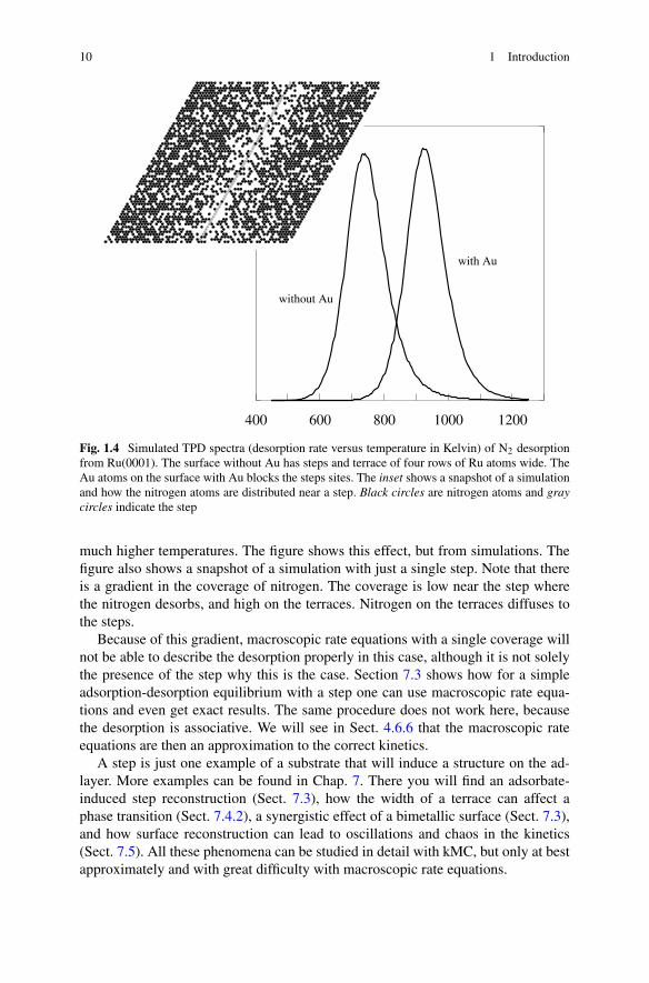
Figure 1.4 shows simulated TPD spectra of a model of N2 desorption fromRu(0001). It was hypothesized that the experimental spectra showed not desorp-tion from a flat surface, but from steps on the surface. Gold was added to the surfaceto block the steps sites and to test this hypothesis [10]. Indeed this shifted the peak to

10 1 Introduction

Fig. 1.4 Simulated TPD spectra (desorption rate versus temperature in Kelvin) of N2 desorptionfrom Ru(0001). The surface without Au has steps and terrace of four rows of Ru atoms wide. TheAu atoms on the surface with Au blocks the steps sites. The inset shows a snapshot of a simulationand how the nitrogen atoms are distributed near a step. Black circles are nitrogen atoms and graycircles indicate the step

much higher temperatures. The figure shows this effect, but from simulations. Thefigure also shows a snapshot of a simulation with just a single step. Note that thereis a gradient in the coverage of nitrogen. The coverage is low near the step wherethe nitrogen desorbs, and high on the terraces. Nitrogen on the terraces diffuses tothe steps.

Because of this gradient, macroscopic rate equations with a single coverage willnot be able to describe the desorption properly in this case, although it is not solelythe presence of the step why this is the case. Section 7.3 shows how for a simpleadsorption-desorption equilibrium with a step one can use macroscopic rate equa-tions and even get exact results. The same procedure does not work here, becausethe desorption is associative. We will see in Sect. 4.6.6 that the macroscopic rateequations are then an approximation to the correct kinetics.

A step is just one example of a substrate that will induce a structure on the ad-layer. More examples can be found in Chap. 7. There you will find an adsorbate-induced step reconstruction (Sect. 7.3), how the width of a terrace can affect aphase transition (Sect. 7.4.2), a synergistic effect of a bimetallic surface (Sect. 7.3),and how surface reconstruction can lead to oscillations and chaos in the kinetics(Sect. 7.5). All these phenomena can be studied in detail with kMC, but only at bestapproximately and with great difficulty with macroscopic rate equations.

1.3 Length and Time Scales 11

1.3 Length and Time Scales

The discussion above has shown that we need to know the structure of the adlayeron an atomic scale to understand the kinetics. To get the rate of the A + B reactionit was necessary to know the number of A–B pairs. On the other hand kinetics isgenerally studied on meso- or macroscopic scales. Atomic scales are of the order ofÅngstrøm and femtoseconds. Typical length scales in laboratory experiments varybetween micrometers to centimeters. The difference in time scales is often evenlarger. Vibrations of molecules have periods in the order of femtoseconds. Somereactions take only nanoseconds, but others seconds to many hours. This means thatthere are many orders of difference in length and time scales between the individualreactions and the resulting kinetics.

The length gap is not always a problem. Many systems are homogeneous, and thekinetics of a macroscopic system can be reduced to the kinetics of a few reactingmolecules. This is generally the case for reactions in the gas phase and in solutions.For reactions on the surface of a catalyst it is not always clear when this is the case.It is certainly the case that in the overwhelming number of studies on the kinetics inheterogeneous catalysis it is implicitly assumed that the adsorbates are well-mixed,and that macroscopic rate equations (1.1) can be used. We have already seen exam-ples of systems that show correlation in the occupation of sites that are close. Theremay however also be ordering on a larger scale. For example, there are systems thatshow pattern formation with a characteristic length scale of micro- to centimeters[11]. For such systems the macroscopic rate equations can be extended by makingthe coverages position dependent: θ = θ(r, t). One generally then also adds a dif-fusion term. The resulting expressions are called reaction-diffusion equations [12].The problem with these equations is however the same as the one with the macro-scopic rate equations. On the atomic length scale the adsorbates are assumed to berandomly distributed, but it is just this assumption that is rarely correct.

The real problem however is the time gap. The typical atomic time scale is givenby the period of a molecular vibration. The fastest vibrations have a reciprocal wave-length of up to 4000 cm−1, and a period of about 8 fs. Reactions in catalysis takeplace in seconds or more. It is important to be aware of the origin of these fifteenorders of magnitude difference. A reaction can be regarded as a movement of thesystem from one local minimum on a potential-energy surface (PES) to another. Insuch a move a so-called activation barrier has to be overcome. Most of the time thesystem moves around one local minimum. This movement is fast, takes place in theorder of femtoseconds, and corresponds to a superposition of all possible vibrations.Every time that the system moves in the direction of the activation barrier can be re-garded as an attempt to react. The probability that the reaction actually succeeds canbe estimated by calculating a Boltzmann factor that gives the relative probability offinding the system at a local minimum or on top of the activation barrier. This Boltz-mann factor is given by exp[−Ebar/kBT ], where Ebar is the height of the barrier.A barrier of Ebar = 100 kJ/mol at room temperature gives a Boltzmann factor ofabout 10−18. Hence we see that the very large difference in time scales is due to thevery small probability that the system overcomes activations barriers.

12 1 Introduction

The standard method to study the evolution of a system on an atomic scale isMolecular Dynamics (MD) [13–15]. In MD a reaction with a high activation barrieris called a rare event, and various techniques have been developed to get a reactioneven when a standard simulation would never show it. These techniques, however,work for one reacting molecule or two molecules that react together, but not whenone is interested in the combination of thousands or more reacting molecules thatone has when studying kinetics. The objective of this book is to show how one dealswith such a collection of reacting molecules. It turns out that one has to sacrificessome of the detailed information that one has in MD simulations. One can still workon atomic length scales, but one cannot work with the exact position of all atomsin a system. Instead one only specifies near which minimum of the PES the systemis. One does not work with the atomic time scale. Instead one has the reactions aselementary events: i.e., one specifies at which moment the system moves from oneminimum of the PES to another. Moreover, because one doesn’t know where theatoms are exactly and how they are moving, one cannot determine the times forthe reactions exactly either. Instead one can only give probabilities for the times ofthe reactions. It turns out, however, that this information is more than sufficient forstudying kinetics. The resulting method is kMC: the topic of this book.

References

1. M. Boudart, Kinetics of Chemical Processes (Prentice Hall, Englewood Cliffs, 1968)2. R.A. van Santen, J.W. Niemantsverdriet, Chemical Kinetics and Catalysis (Plenum, New York,

1995)3. J.A. Dumesic, D.F. Rudd, L.M. Aparicio, The Microkinetics of Heterogeneous Catalysis (Am.

Chem. Soc., Washington, 1993)4. C.G.M. Hermse, A.P.J. Jansen, in Catalysis, vol. 19, ed. by J.J. Spivey, K.M. Dooley (Royal

Society of Chemistry, London, 2006)5. R.M. Ziff, E. Gulari, Y. Barshad, Phys. Rev. Lett. 56, 2553 (1986)6. A.P.J. Jansen, Phys. Rev. B 69, 035414 (2004)7. R.J. Baxter, Exactly Solved Models in Statistical Mechanics (Academic Press, London, 1982)8. W.K. Offermans, A.P.J. Jansen, R.A. van Santen, Surf. Sci. 600, 1714 (2006)9. C. Wu, D.J. Schmidt, C. Wolverton, W.F. Schneider, J. Catal. 286, 88 (2012)

10. S. Dahl, A. Logadottir, R.C. Egeberg, J.H. Larsen, I. Chorkendorff, E. Törnqvist, J.K.Nørskov, Phys. Rev. Lett. 83, 1814 (1999)

11. R. Imbihl, G. Ertl, Chem. Rev. 95, 697 (1995)12. P. Grindrod, The Theory and Applications of Reaction-Diffusion Equations: Patterns and

Waves (Clarendon, Oxford, 1996)13. M.P. Allen, D.J. Tildesley, Computer Simulation of Liquids (Clarendon, Oxford, 1987)14. D. Frenkel, B. Smit, Understanding Molecular Simulation: From Algorithms to Applications

(Academic Press, London, 2001)15. D.C. Rapaport, The Art of Molecular Dynamics Simulation (Cambridge University Press,

Cambridge, 2004)

Chapter 2A Stochastic Model for the Descriptionof Surface Reaction Systems

Abstract The most important concept for surface reactions is the adsorption site.For simple crystal surfaces the adsorption sites form a lattice. Lattices form the basisfor the description of surface reactions in kinetic Monte Carlo. We give the defini-tion of a lattice and discuss related concepts like translational symmetry, primitivevectors, unit cells, sublattices, and simple and composite lattices. Labels are intro-duced to describe the occupation of the adsorption sites. This leads to lattice-gasmodels. We show how these labels can be used to describe reactions and other sur-faces processes and we make a start with showing how they can also be used tomodel surfaces that are much more complicated than simple crystal surfaces. Ki-netic Monte Carlo simulates how the occupation of the sites changes over time. Wederive a master equation that gives us probability distributions for what processescan occur and when these processes occur. The derivation is from first principles.Some general mathematical properties of the master equation are discussed and weshow how a lattice-gas model simplifies the master equation so that it becomes fea-sible to use it as a basis for kinetic Monte Carlo simulations.

2.1 The Lattice Gas

We start the discussion of the way how we will model surface reactions by spec-ifying how we will describe our systems. We want an atomic scale description ofour systems and relate this to the macroscopic kinetics: i.e., we want to be able totalk about individual atoms and molecules reacting on a surface, and then link thisto global changes and reaction rates of the layer of adsorbates. It turns out that theproper way to described a system is related to the different time scales with whichthings change on the atomic and on the macroscopic scale. We will see that we needto do some coarse-graining on the atomic length scale to bridge the gap in timescales.

If we regard the evolution of a layer of atoms and molecules adsorbed on a sur-face on an atomic scale, we will notice that there is a huge difference in time scaleof the motion of individual atoms and molecules on the one and of the macroscopicproperties on the other hand. For most systems of interest in catalysis, for example,the latter typically vary over a period of seconds or even longer. Motions of atomsoccur typically on a time scale of femtoseconds. This enormous gap in time scales

A.P.J. Jansen, An Introduction to Kinetic Monte Carlo Simulations of SurfaceReactions, Lecture Notes in Physics 856,DOI 10.1007/978-3-642-29488-4_2, © Springer-Verlag Berlin Heidelberg 2012

13

14 2 A Stochastic Model for the Description of Surface Reaction Systems

poses a large problem if we want to predict or even explain the kinetics (i.e., reactionrates) in terms of the processes that take place on the atomic scale.

The conventional method to simulate the motions of atoms and molecules isMolecular Dynamics (MD) [1–3]. This method generally discretizes time in inter-vals of equal lengths. The size of this so-called time step, and with it the compu-tational costs, is determined by the fast vibrations of chemical bonds [1]. A stretchvibration of a C-H bond has a typical frequency of around 3000 cm−1. This cor-responds to a period of about 10 fs. If one wants to study the kinetics of surfacereactions, then one needs a method that does away with these fast motions.

The kinetic Monte Carlo (kMC) method that we present here does this by us-ing the concept of sites. The forces working on an atom or a molecule that adsorbson a surface move it to well-defined positions on the surface [4, 5]. These posi-tions are called sites. They correspond to minima on the potential-energy surface(PES) for the adsorbate. Most of the time adsorbates stay very close to these min-ima. If we would take a snapshot of a layer of adsorbates at normal temperatures,only about 1 in 1013 of them would not be near a minimum at normal reactionconditions. Only when they diffuse from one site to another or during a reactionthey will not be near such a minima, but only for a very short time. Now insteadof specifying the precise positions, orientations, configurations, and motions of theadsorbates we will only specify for each sites its occupation. A reaction and a diffu-sion from one site to another will be modeled as a sudden change in the occupationof the sites. These changes are the elementary events in a kMC simulation. Thevibrations of the adsorbates do not change the occupations of the sites. So theyare not simulated in kMC, and hence they do not determine the time scale of akMC simulation. Reactions and diffusion take place on a much longer time scale.Thus by taking a slightly larger length scale, we can simulate a much longer timescale.

If the surface has two-dimensional translational symmetry, or when it can bemodeled as such, the sites form a regular grid or a lattice. Our model is then a so-called lattice-gas model. This chapter shows how this model can be used to describea large variety of problems in the kinetics of surface reactions.

2.1.1 Lattices, Sublattices, and Unit Cells

If the surface has two-dimensional translational symmetry then there are two lin-early independent vectors, a1 and a2, with the property that when the surface istranslated over any of these vectors the result is indistinguishable from the situationbefore the translation. It is said that the system is invariant under translation overthese vectors. In fact the surface is then invariant under translations for any vectorof the form

n1a1 + n2a2 (2.1)

where n1 and n2 are integers. If all translations that leave the surface invariant canbe written as (2.1), then a1 and a2 are so-called primitive vectors or primitive trans-

2.1 The Lattice Gas 15

lations, and the vectors of the form (2.1) are the lattice vectors. Primitive vectors arenot uniquely defined. For example a (111) surface of a fcc metal is translationallyinvariant for a1 = a(1,0) and a2 = a(1/2,

√3/2), where a is the lattice spacing.

But one can just as well choose a1 = a(1,0) and a2 = a(−1/2,√

3/2). The areadefined by

x1a1 + x2a2 (2.2)

with x1, x2 ∈ [0,1〉 is called the unit cell. The whole system is obtained by tiling theplane with the contents of a unit cell.

Expression (2.1) defines a simple lattice, Bravais lattice, or net. Simple latticeshave just one lattice point, or grid point, per unit cell. It is also possible to have morethan one lattice point per unit cell. The lattice is then given by all points

s(i) + n1a1 + n2a2 (2.3)

with i = 0,1, . . . ,Nsub − 1 and Nsub the number of lattice points in the unit cell.Each s(i) is a different vector in the unit cell. The set s(i) + n1a1 + n2a2 for a par-ticular vector i forms a sublattice, which is itself a simple lattice. There are Nsubsublattices, and they are all equivalent: they are only translated with respect to eachother. (For more information on lattices, also for a discussion of their symmetry, seefor example references [4] and [6].) All points of the form (2.3) from a compositelattice.

The sites of a simple crystal surface form a lattice. The description so far sug-gests that the different lattice points in a unit cell, corresponding to sites, are all in thesome plane, but that does not need to be the case. As we will see in Sect. 4.6.3, thatdifferent lattice points may also correspond to positions for adsorbates in differentlayers that are stacked on top of each other. Lattices can also be used to model sur-faces that are much more complicated than simple crystal surfaces (see Sects. 5.5.2and 5.5.3). In fact, we will see that sometimes lattice points do not correspond tophysical adsorption sites at all (see Sect. 5.5.4).

2.1.2 Examples of Lattices

Figure 2.1 shows top and hollow sites of the (100) surface of an fcc metal. Such asurface has a1 = a(1,0) and a2 = a(0,1) as primitive translations with a the dis-tance between the surface atoms. CO for example prefers the top sites on such sur-face if the metal is rhodium [7–10]. We have Nsub = 1 if we would only includethese top sites. We can choose the origin of our reference frame any way we wantso we take s(0) = (0,0) for simplicity. If we would want to include the hollow sitesas well then Nsub = 2 and s(1) = a(1/2,1/2).

Figure 2.2 shows bridge sites of the same surface. Some CO moves to thesebridge sites at high coverages [7–10]. If we would include the top and bridge sitesto describe all adsorption sites for CO/Rh(100), then we would have Nsub = 3 ands(0) = (0,0), s(1) = a(1/2,0), and s(2) = a(0,1/2) for the top and the two types ofbridge site, respectively.

16 2 A Stochastic Model for the Description of Surface Reaction Systems

Fig. 2.1 The large whitecircles with gray edges depictthe atoms of the top layer of a(100) surface of an fcc metal.The black circles indicate thepositions of the top sites, andthe gray circles with blackedges the positions of thehollow sites. The top sitesform a simple lattice as do thehollow sites. In the top-leftcorner the unit cell and theprimitive translations of thesurface are shown

Figure 2.3 shows a (111) surface of an fcc metal. CO on Pt prefers to adsorb onthis surface on the top sites [4]. We can therefore model CO on this surface with asimple lattice with the lattice points corresponding to the top sites. We have a1 =a(1,0) and a2 = a(1/2,

√3/2). As Nsub = 1 we choose the origin of our reference

frame so that s(0) = (0,0) for simplicity. Each lattice point corresponds to a site thatis either vacant or occupied by CO.

NO on Rh(111) forms a (2 × 2)-3NO structure in which equal numbers of NOmolecules occupy top, fcc hollow, and hcp hollow sites [11, 12]. Figure 2.3 showsall the sites that are involved. We now have three sublattices with s(0) = (0,0) (top

Fig. 2.2 The large white circles with gray edges depict the atoms of the top layer of a (100) surfaceof an fcc metal. The black circles and the gray circles with black edges indicate the positions ofthe bridge sites. Although all bridge sites have the same adsorption properties, together they do notform a simple lattice, but a composite lattice. This is because the relative positions of the surfaceatoms with respect to the “black” bridge sites is different from those of the “gray” bridge sites.However, if we ignore the surface atoms, then all bridge sites together from a square simple lattice.In the top-left corner the unit cell and the primitive translations of the surface are shown

2.1 The Lattice Gas 17

Fig. 2.3 The large white circles with gray edges depict the atoms of the top layer of a (111) surfaceof an fcc metal. The black circles indicate the positions of the top sites, and the gray circles withblack edges the positions of one type of hollow site, say fcc, and the small white circle with blackedges the positions of the other type, say hcp, of hollow site. The top sites form a simple lattice asdo the fcc sites and the hcp sites separately. The top and hollow sites together also form a simplelattice if we disregard the different adsorption properties of the sites and the different positionswith respect to the surface atoms. Otherwise they form a composite lattice with three sublattices.In the top-left corner the unit cell and the primitive translations of the surface are shown

Fig. 2.4 The large whitecircles with gray edges depictthe atoms of the top layer of a(111) surface of an fcc metal.The black circles, the graycircles with black edges, andthe small white circle withblack edges indicate thepositions of the bridge sites.Together they form acomposite lattice even thoughthey have the same adsorptionproperties. In the top-leftcorner the unit cell and theprimitive translations of thesurface are shown

sites), s(1) = a(1/2,√

3/6) (fcc hollow sites), and s(2) = a(1,√

3/3) (hcp hollowsites).

At high coverages the repulsion between the CO molecules on Pt(111) forcessome of them again to bridge sites [13]. Figure 2.4 shows the bridge sites. We havenow four sublattices with s(0) = (0,0), s(1) = a(1/2,0), s(2) = a(1/4,

√3/4), s(3) =

a(3/4,√

3/4). The first one is for the top sites (not shown in the figure, but seeFig. 2.3). The others are for the three sublattices of bridge sites. The four sublattices

18 2 A Stochastic Model for the Description of Surface Reaction Systems

together form a simple lattice, but only when we do not distinguish between top andbridge sites.

The examples here are of simple single crystal surfaces. It would be wrong how-ever to assume that a lattice-gas model can only be used for such surfaces. The unitcell can be much larger and with many more sites. This makes it possible to modela surface with steps. But it is even possible to model systems with no translationalsymmetry at all with a lattice-gas model. It is possible to model steps at variabledistances, point defects, bimetallic surfaces, and many more systems through theuse of labels as explained in Sect. 2.1.3.

2.1.3 Labels and Configurations

The sites are the positions where the adsorbates are found on the surface, but foreach site we need something to indicate if it is occupied or not, and if it is occupiedwith which adsorbate. We use labels for this.

We assign a label to each lattice point. The lattice points correspond to the sites,and the labels specify properties of the sites. A particular labeling of all lattice pointstogether we call a configuration. The most common property that one wants to de-scribe with the label is the occupation of the site. We use the short-hand notation(n1, n2/s : A) to mean that the site at position s(s) + n1a1 + n2a2 is occupied by anadsorbate A.

The labels are also used to specify reaction. A reaction can be regarded as nothingbut a change in the labels. An extension of the short-hand notation (n1, n2/s : A →B) indicates that during a reaction the occupation of the site at s(s) + n1a1 + n2a2changes from A to B. If more than one site is involved in a reaction then the spec-ification will consist of a set changes of the form (n1, n2/s : A → B). Not only re-actions can be specified in this way. Also other processes can be described like this.For example, a diffusion of an adsorbate A might be specified by {(0,0/0 : A →∗), (1,0/0 :∗ → A)}. Here ∗ stands for a vacant site, and the diffusion is from sites(0) to s(0) + a1. We will also write this as (0,0/0), (1,0/0) : A∗ → ∗A.

There are many other uses for labels as will be discussed in Sect. 2.1.4 andChaps. 5, 6, and 7. Most kMC programs are special-purpose codes with hard cod-ing of the processes. Labels play only a minor role in these programs. Labels arehowever an important and very versatile tool in general-purpose kMC codes. Theyallow great flexibility in creating models for reaction systems, and a clever use ofthem can greatly enhance the speed of simulations.

2.1.4 Examples of Using Labels

Desorption of CO from Pt(111) can be written as (0,0 : CO → ∗) when we use amodel of the top sites shown in Fig. 2.3. We have left out the index of the sublattice,

2.1 The Lattice Gas 19

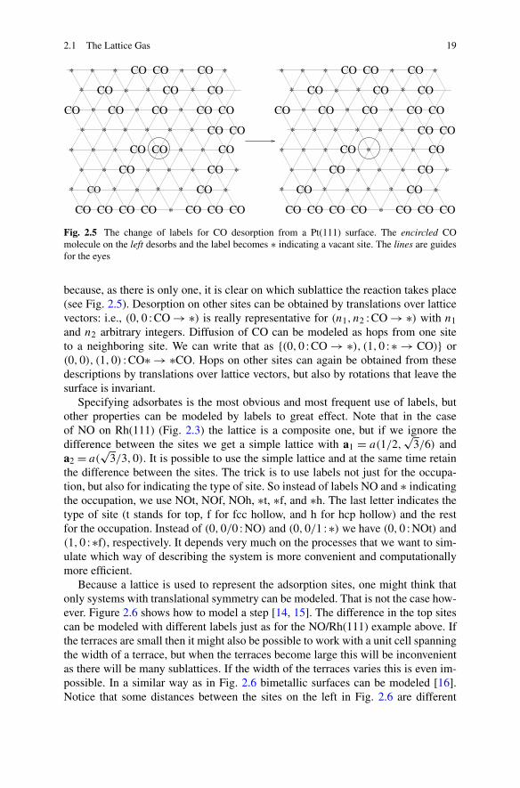
Fig. 2.5 The change of labels for CO desorption from a Pt(111) surface. The encircled COmolecule on the left desorbs and the label becomes ∗ indicating a vacant site. The lines are guidesfor the eyes

because, as there is only one, it is clear on which sublattice the reaction takes place(see Fig. 2.5). Desorption on other sites can be obtained by translations over latticevectors: i.e., (0,0 : CO → ∗) is really representative for (n1, n2 : CO → ∗) with n1and n2 arbitrary integers. Diffusion of CO can be modeled as hops from one siteto a neighboring site. We can write that as {(0,0 : CO → ∗), (1,0 :∗ → CO)} or(0,0), (1,0) : CO∗ → ∗CO. Hops on other sites can again be obtained from thesedescriptions by translations over lattice vectors, but also by rotations that leave thesurface is invariant.

Specifying adsorbates is the most obvious and most frequent use of labels, butother properties can be modeled by labels to great effect. Note that in the caseof NO on Rh(111) (Fig. 2.3) the lattice is a composite one, but if we ignore thedifference between the sites we get a simple lattice with a1 = a(1/2,

√3/6) and

a2 = a(√

3/3,0). It is possible to use the simple lattice and at the same time retainthe difference between the sites. The trick is to use labels not just for the occupa-tion, but also for indicating the type of site. So instead of labels NO and ∗ indicatingthe occupation, we use NOt, NOf, NOh, ∗t, ∗f, and ∗h. The last letter indicates thetype of site (t stands for top, f for fcc hollow, and h for hcp hollow) and the restfor the occupation. Instead of (0,0/0 : NO) and (0,0/1 :∗) we have (0,0 : NOt) and(1,0 :∗f), respectively. It depends very much on the processes that we want to sim-ulate which way of describing the system is more convenient and computationallymore efficient.

Because a lattice is used to represent the adsorption sites, one might think thatonly systems with translational symmetry can be modeled. That is not the case how-ever. Figure 2.6 shows how to model a step [14, 15]. The difference in the top sitescan be modeled with different labels just as for the NO/Rh(111) example above. Ifthe terraces are small then it might also be possible to work with a unit cell spanningthe width of a terrace, but when the terraces become large this will be inconvenientas there will be many sublattices. If the width of the terraces varies this is even im-possible. In a similar way as in Fig. 2.6 bimetallic surfaces can be modeled [16].Notice that some distances between the sites on the left in Fig. 2.6 are different

20 2 A Stochastic Model for the Description of Surface Reaction Systems

Fig. 2.6 A Ru(0001) surface with a step with the top sites indicated on the left. On the right isshown the lattice. The large open circles are the atoms. The small open circles indicate top sites onthe terraces, the small black circles top sites at the bottom of the step, and the small gray circlestop sites at the top of the step. Notice the difference in distance between the top sites at the step onthe left and on the right

from those on the right. The distance between the sites on the top and bottom of astep is smaller on the left than on the right. On the right this distance is increasedso that the sites form a lattice. Such a distortion of the system is quite acceptable inkMC simulations. The elementary events (reactions, diffusion, and possibly otherprocesses) are described in terms of changes of the labels of sites. We only need toknow which sites and how the labels change. Distances between sites are not part ofthe description of events.

Site properties like the sublattice of which the site is part of and if it is a stepsite or not are static properties. The occupation of a site is a dynamic property.There are also other properties of sites that are dynamic. Bare Pt(100) reconstructsinto a quasi-hexagonal structure [17]. CO oxidation on Pt(100) is substantially in-fluenced by this reconstruction because oxygen adsorbs much less readily on thereconstructed surfaces than on the unreconstructed one. This can lead to oscilla-tions, chaos, and pattern formation [17, 18]. It is possible to model the effect ofthe reconstruction on the CO oxidation by using a label that specifies whether thesurface is locally reconstructed or not [19–21].

Chapters 5, 6, and 7 will show more esoteric uses of labels. Labels can be usedas flags or as counters as well. Very often this use is combined with fictitious pro-cesses and fictitious sites, which can either be a way of modeling actual physicaland chemical processes, or a way to get kinetic information.

2.1.5 Shortcomings of Lattice-Gas Models

The lattice-gas model is simple yet very powerful, as it allows us to model a largevariety of systems and phenomena. Still, not everything can be modeled with it.

2.1 The Lattice Gas 21

Let’s look again at CO oxidation on Pt(100). As stated above this system showsreconstruction which can be modeled with a label indicating that the surface is re-constructed or not. This way of modeling has shown to be very successful [19–21],but it does neglect some aspects of the reconstruction. The reconstructed and the un-reconstructed surface have very different unit cells, and the adsorption sites are alsodifferent [22, 23]. In fact, the unit cell of the reconstructed surface is very large, andthere are a large number of adsorption sites with slightly different properties. Theseaspects have been neglected in the kinetic simulations so far. As these simulationshave been quite successful, it seems that these aspects are not very relevant in thiscase, but that need not always be so. Another example would be catalytic partialoxidation (CPO), which takes place at high temperatures at which the surface is sodynamic that all translational symmetry is lost. In this case using a lattice to modelthe kinetics seems inappropriate.

The example of CO on Pt(111) has shown that at high coverage the position atwhich the molecules adsorb change. The reason for this is that these positions arenot only determined by the interactions between the adsorbates and the substrate,but also by the interactions between the adsorbates themselves. At low coveragesthe former dominate, but at high coverages the latter may be more important. Thismay lead to adlayer structures that are incommensurate with the substrate [4]. Ex-amples are formed by the nobles gases. These are weakly physisorbed, whereasat high coverages the packing onto the substrate is determined by the steric re-pulsion between them. At low and high coverages different lattices are needed todescribe the positions of the adsorbates, but a single lattice describing both thelow and the high coverage sites is not possible. Simulations in which the cov-erages change in such a way from low to high coverage and/or vice versa thencannot be based on a lattice-gas model except by making substantial approxima-tions.

Although not all systems can be modeled well by a lattice gas, it is a much moreflexible model than might initially appear. Figure 2.6 already shows some of thisflexibility. Note that the sites in the system in the figure have only translationalsymmetry in the direction parallel to the step, whereas in the corresponding lattice-gas model there is the usual two-dimensional periodicity. This is accomplished bydisplacing the sites at the step somewhat from their real positions. As has beenexplained above, this is perfectly acceptable. Similarly, it is possible to describewith a lattice-gas model a layer of adsorbates that have been displaced from theirnormal site positions by the interactions between them, and that have formed anadlayer with a structure that is incommensurate with that of the preferred adsorp-tion sites. The reason for this flexibility is the labels that we attach to each latticepoint. It will be shown in Chaps. 5, 6, and 7 that these labels make it possible tomodel a very large variety of systems with a lattice gas. Whether or not a sys-tem can be described by a lattice-gas model depends very much on one’s ingenu-ity.

22 2 A Stochastic Model for the Description of Surface Reaction Systems

2.1.6 Boundary Conditions

The surface of a real catalyst will very often contain many more sites than we caninclude in a kMC simulation. In fact, such a surface is generally regarded as infinitein two directions. In a kMC simulation we need to restrict ourselves to a much morelimited number of sites. It is possible to do kMC simulations with all sites in a smallpart of the catalyst’s surface. This gives an acceptable description except for the sitesat the edge. It is more customary to use periodic boundary conditions. In that caseall sites s(i) +n1a1 +n2a2 with n1 = 0,1, . . . ,N1 − 1 and n2 = 0,1, . . . ,N2 − 1 areexplicitly included in the simulation. Sites with values of n1 and/or n2 outside thisrange are thought to have the same label as those of n1 modN1 and n2 modN2. Thesystem can be thought as if being rolled up on a torus. The values of N1 and N2 inreal simulations vary. Sometimes they can be smaller than 100, but simulations withN1 = N2 = 8192 have been reported as well [24].

2.2 The Master Equation

2.2.1 The Definition and Some Properties of the Master Equation

The derivation of the algorithms and a large part of the interpretation of the resultsof kMC simulations are based on a master equation

dPα

dt=∑

β

[WαβPβ − WβαPα]. (2.4)

In this equation t is time, α and β are configurations of the adlayer (i.e., differentways in which adsorbates are distributed over the sites, or more generally ways inwhich labels can be assigned to lattice points), Pα and Pβ are their probabilities,and Wαβ and Wβα are so-called transition probabilities per unit time that specify therate with which the adlayer changes due to reactions and other processes. The mas-ter equation is the single most important equation in kMC. It relates everything thatwe do in kinetics to each other as will be shown below. Here we start with lookingat some of its mathematical properties. The master equation is a loss-gain equa-tion. The first term on the right stands for increases in Pα because of processes thatchange other configurations into α. The second term stands for decreases becauseof processes in α. From

d

dt

∑

α

Pα =∑

α

dPα

dt=∑

αβ

[WαβPβ − WβαPα] = 0 (2.5)

we see that the total probability is conserved. (The last equality can be seen byswapping the summation indices in one of the terms.)

The master equation can be derived from first principles as will be shown below,and hence forms a solid basis for all subsequent work. There are other advantages

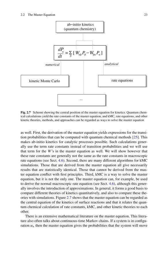
2.2 The Master Equation 23

Fig. 2.7 Scheme showing the central position of the master equation for kinetics. Quantum chem-ical calculations yield the rate constants of the master equation, and kMC, rate equations, and otherkinetic theories, methods, and approaches can be regarded as ways to solve the master equation

as well. First, the derivation of the master equation yields expressions for the transi-tion probabilities that can be computed with quantum chemical methods [25]. Thismakes ab-initio kinetics for catalytic processes possible. Such calculations gener-ally use the term rate constants instead of transition probabilities and we will usethat term for the W ’s in the master equation as well. We will show however thatthese rate constants are generally not the same as the rate constants in macroscopicrate equations (see Sect. 4.6). Second, there are many different algorithms for kMCsimulations. Those that are derived from the master equation all give necessarilyresults that are statistically identical. Those that cannot be derived from the mas-ter equation conflict with first principles. Third, kMC is a way to solve the masterequation, but it is not the only one. The master equation can, for example, be usedto derive the normal macroscopic rate equation (see Sect. 4.6), although this gener-ally involves the introduction of approximations. In general, it forms a good basis tocompare different theories of kinetics quantitatively, and also to compare these the-ories with simulations. Figure 2.7 shows that the master equation can be regarded asthe central equation of the kinetics of surface reactions and that it relates the quan-tum chemical calculation of rate constants, kMC, and other kinetic theories to eachother.

There is an extensive mathematical literature on the master equation. This litera-ture also often talks about continuous-time Markov chains. If a system is in configu-ration αn then the master equation gives the probabilities that the system will move

24 2 A Stochastic Model for the Description of Surface Reaction Systems

to another configuration αn+1. These probabilities do not depend on the configura-tions that the system was in before αn. This makes αn → αn+1 a Markov process[26, 27]. Continuing the transitions from one configuration to another gives a seriesαn → αn+1 → αn+2 → . . . that is called a Markov chain.

We discuss here only a few basic properties [26, 27]. The reader should be awarehowever that even these properties have only a limited use in relation to kMC sim-ulations and should not be overinterpreted. For example, the Ziff–Gulari–Barshad(ZGB) model of CO oxidation has been extensively studied with kMC simulations(see Sect. 7.4.3). The physics literature mentions three states. Two of these statescorrespond to CO poisoning and oxygen poisoning of the surface. The third corre-sponds to a reactive state. The point here is that strictly speaking this reactive stateis not stable. This means that it can not represent a steady state. The ZGB modelmight therefore seem a rather useless model for CO oxidation. However, the time ittakes for the reactive state to turn into one of the poisoning states is so enormouslylong, even for small system sizes, that it can effectively be regarded as a stable state.This is what is actually done in the literature.

We start with a discussion of the class structure [27]. Suppose we mean by α → β

that there is a chain of processes that can convert configuration α into β . (Notethat we normally use this notation to indicate a change of configuration by a singleprocess.) We then define α ↔ β to mean α → β and β → α. This relation ↔ definesan equivalence relation [28]. This means α ↔ α for all α, if α ↔ β then β ↔ α, andif α ↔ β and β ↔ γ then α ↔ γ . Because of these properties we can partition allconfigurations into equivalence classes: i.e., α and β belong to the same class if andonly if α ↔ β .

A class is closed if α is in the class and α → β implies that β is also in the sameclass as α: i.e., β → α also holds. If the system ends up in a closed class, then itwill never leave it. Such a situation may for example arise when no reactions arepossible in a system anymore, and the adsorbates can only hop from one site toanother. A system in a closed class visits each of the configurations in the class aninfinite number of times. This does not hold for configurations in a class that is notclosed. If a closed class consists of a single configuration, then the configuration iscalled an absorbing state. The poisoned states mentioned above for the ZGB modelare examples of such absorbing states.

If all configurations can be partitioned into two or more sets such that neitherα → β nor β → α holds if α and β are in different sets, then the system is saidto be reducible or decomposable. This terminology is related to the way in whichthe master equation can be written in matrix-vector form. With the vector P withcomponents Pα = Pα , and the matrix W with components

Wαβ ={

Wαβ, if α = β, and−∑γ Wγβ, if α = β, (2.6)

we can write the master equation as

P = WP. (2.7)

2.2 The Master Equation 25

For a completely reducible or decomposable system the matrix W can be written inthe form

(A 00 B

)(2.8)

with A and B square matrices by appropriately ordering the configurations. Theconfigurations in the different sets can be treated completely independently fromeach other. A system that is not reducible is called irreducible.

If there is a closed class, but the system is irreducible, then we can write W inthe form

(A D0 B

)(2.9)

with D a non-zero matrix, A and B square matrices, and the rows and columns ofA indexed by the configurations in the closed class. Such a system is called (incom-pletely) reducible. If there are two closed classes, then W can be written as

(A 0 D0 B E0 0 C

)(2.10)

with A, B, and C square matrices, D and E non-zero matrices, and the rows andcolumns of A and B being indexed by the configurations in the two closed classes.Such a system is called splitting, because it ends up in one closed class or the other.

The definition of W immediately gives∑

α

Wαβ = 0. (2.11)

Matrices with this property can be shown to have at least one right eigenvector witheigenvalue equal to zero [26]. The components of such eigenvector are all non-negative and by proper normalization can be identified with the probabilities to findthe system in a configuration when the system is in a steady state. It can also beshown that the system will evolve toward such an eigenvector.

There are various ways to prove this [26]. One way is to write the solution of themaster equation as

P(t) = eWtP(0), (2.12)

where P(0) are the probabilities of the configurations at t = 0. If we can diagonalizeW and write

WU = UV, (2.13)

then this becomes

P(t) = UeVtU−1P(0). (2.14)

The matrix V is diagonal and all matrix elements on the diagonal are non-positive.This means that for large t , all components of exp[Vt] vanish, except those withzero on the diagonal of V. P evolves to the corresponding eigenvector in U.

26 2 A Stochastic Model for the Description of Surface Reaction Systems

Note that an eigenvector with eigenvalue equal to zero does not exclude the exis-tence of an oscillation. Suppose we have configurations α1, α2, . . . , αN with N ≥ 2and the system always moves from αn directly to αn+1 for n = 1,2, . . . ,N − 1 andfrom αN directly to α1. This means that we have a cycle. The eigenvector with zeroeigenvalue has Wαn+1αnPαn = Wα1αN

PN for n = 1,2, . . . ,N − 1. Although the sys-tem has a cycle, this can still be regarded as a stationary state because the time ittakes the system to move through the cycle will not always be exactly the same. Itcan be shown (see Sect. 3.7.3) that on average this will take a time equal to

T =N−1∑

n=1

W−1αn+1αn

+ W−1α1αN

. (2.15)

If we would start the system in α1 at time t = 0 and follow the system, then after atime T we would find it most likely again in α1, but also with some small probabilityin αN and α2, with an even smaller probability in αN−1 and α3, et cetera. After an-other period T the probability of finding the system in α1 would be reduced and theprobabilities for configurations before and after α1 would be increased. After manyperiods T we would find the system in one of the configurations with a probabilitycorresponding to the one given by the eigenvector with zero eigenvalue.

2.2.2 The Derivation of the Master Equation

The master equation can be derived by looking at the surface and its adsorbatesin phase space.1 This is, of course, a classical mechanics concept, and one mightwonder if it is correct to look at the processes on an atomic scale and use classicalmechanics. The situation here is the same as for the derivation of the rate equationsfor gas phase reactions. The usual derivations there also use classical mechanics[29–33]. Although it is possible to give a completely quantum mechanical derivationformalism [34–37], the mathematical complexity hides much of the important partsof the chemistry. We therefore give only a classical derivation. It is possible at theend to replace the classical expressions by quantum mechanical ones, in exactly thesame way as for gas phase reactions. The new expressions will depend on the typeof motion (vibration, rotation, et cetera). This will be shown in detail in Chap. 4.

The derivation of the master equation is usually based on the observation thatthere is a separation between the time scale on which reactions take place and thetime scale of much faster motions like vibrations [38, 39]. The longer time scale ofreactions defines states, in which the system is localized in configuration space, andthe transitions between them can be described by a master equation. The rates ofthe individual transitions can each be computed separately by one of the methods

1Parts of Sect. 2.2.2 have been reprinted with permission from X.Q. Zhang, A.P.J. Jansen, Ki-netic Monte Carlo method for simulation reactions in solutions, Phys. Rev. E 82, 046704 (2010).Copyright 2010, American Physical Society.

2.2 The Master Equation 27

of chemical kinetics: e.g., Transition-State Theory (TST) [38–40]. We present herea different derivation that incorporates all process at the same time [41–43]. It is ageneralization of the derivation of Variational TST (VTST): i.e., we partition phasespace in many regions [29, 32, 33], and it is an alternative to the derivation usingprojection operators [44, 45]. It has the advantage that the result is somewhat moregeneral. We will use this in Sects. 2.2.3 and 8.2. The derivation does not use the factthat we are interested in surface reactions, and has a much more general validity. Wewill show in Sect. 2.2.3 how the results simplify for surface reactions.

A point in phase space completely specifies the positions and momenta of allatoms in the system. In MD simulations one uses these positions and momenta atsome starting point to compute them at later times. One thus obtains a trajectory ofthe system in phase space. We are not interested in that amount of detail, however.In fact, as was stated before, too much detail is detrimental if one is interested insimulating many processes. The time interval that one can simulate a system usingMD is typically of the order of nanoseconds. Reactions in catalysis have a charac-teristic time scale that is many orders of magnitude longer. To overcome this largedifference we need an approach that removes the fast processes (vibrations) that de-termine the time scale of MD, and leaves us with the slow processes (reactions).This approach looks as follows.

Instead of the precise position of each atom, we only want to know how the dif-ferent adsorbates are distributed over the sites of a surface. So our physical modelis a lattice. Each lattice point corresponds to one site, and has a label that specifieswhich adsorbate is adsorbed. (A vacant site is simply a special label.) This gives us aconfiguration. As each point in phase space is a precise specification of the positionof each atom, we also know which adsorbates are at which sites: i.e., we know thecorresponding configuration. Different points in phase space may, however, corre-spond to the same configuration. These points differ only in slight variations of thepositions and momenta of the atoms. This means that we can partition phase spacein many regions, each of which corresponds to one configuration. The processesare then nothing but the motion of the system in phase space from one region toanother.

More generally and in line with the idea of different time scales mentioned above,we can start with identifying the regions in configuration space where the fast mo-tions take place. Figure 2.8 shows a sketch of a PES of an arbitrary system. Weassume that only the electronic ground state is relevant, so that the PES is a single-valued function of the positions of all the atoms in the system. The points in thefigure indicate the minima of the PES. Each minimum of the PES has a catchmentregion. This is the set of all points that lead to the minimum if one follows thegradient of the PES downhill [46].

We now partition phase space into these catchment regions and then extend eachcatchment region with the momenta. Let’s call C the configuration space of a systemand P its phase space [47, 48]. The minima of the PES are points in configurationspace. We define Cα to be the catchment region of minimum α. This catchment

28 2 A Stochastic Model for the Description of Surface Reaction Systems

Fig. 2.8 A sketch of a potential-energy surface of an arbitrary system and its corresponding graph.The points are minima of the potential-energy surface. The edges in the graph connect minima thathave catchment regions that border on each other. They correspond to reactions or other activatedprocesses

region is a subspace of configuration space C, and all catchment regions form apartitioning of the configuration space.

C =⋃

α

Cα. (2.16)

(There is a small difficulty with those points of configuration space that do notlead to minima, but to saddle points, and with maxima. These points are irrelevantbecause the number of such points are vanishing small with respect to the otherpoints. They are found where two or more catchment regions meet, and we canarbitrarily assign them to one of these catchment regions.) With q the set of allcoordinates and p the set of all conjugate momenta we can extend the catchmentregion Cα to a corresponding region in phase space Rα as follows.

Rα = {(q,p) ∈ P|q ∈ Cα

}. (2.17)

We then have for phase space

P =⋃

α

Rα. (2.18)

If we use the regions Rα , we can derive the master equation exactly as for the lattice-gas model. This starting point based on the PES for the derivation of the masterequation is more general than the one that defines the regions in phase space interms of configurations of adlayers. It applies in principle to any molecular system.However, for an adlayer both lead to the same partitioning of phase space.

The probability to find the system in region Rα is given by

Pα(t) =∫

Rα

dqdphD

ρ(q,p, t), (2.19)

2.2 The Master Equation 29

where h is Planck’s constant, D is the number of degrees of freedom, and ρ isthe phase space density. The denominator hD is not needed for a purely classicaldescription of the kinetics. However, it makes the transition later on from a classicalto a quantum mechanical description easier [47].

The master equation tells us how these probabilities Pα change in time. Differ-entiating Eq. (2.19) yields

dPα

dt=∫

Rα

dqdphD

∂ρ

∂t(q,p, t). (2.20)

This can be transformed using the Liouville-equation [48]

∂ρ

∂t= −

D∑

i=1

[∂ρ

∂qi

∂H

∂pi

− ∂ρ

∂pi

∂H

∂qi

](2.21)

into

dPα

dt=∫

Rα

dqdphD

D∑

i=1

[∂ρ

∂pi

∂H

∂qi

− ∂ρ

∂qi

∂H

∂pi

], (2.22)

where H is the system’s classical Hamiltonian. To simplify the mathematics, wewill assume that the coordinates are Cartesian and the Hamiltonian has the usualform

H =D∑

i=1

p2i

2mi

+ V (q), (2.23)

where mi is the mass corresponding to coordinate i. The area Rα has been definedabove by coordinates only, and the limits of integration for the momenta are ±∞.Although Rα can be defined more generally (we would like to mention reference[49] for a more general derivation), the definition here allows us to go from phasespace to configuration space. The first term on the right-hand-side of Eq. (2.22) nowbecomes∫

Rα

dqdphD

D∑

i=1

∂ρ

∂pi

∂H

∂qi

=D∑

i=1

∫

Rα

dq∂V

∂qi

∫ ∞

−∞dphD

∂ρ

∂pi

=D∑

i=1

∫

Rα

dq∂V

∂qi

∫ ∞

−∞dp1 . . . dpi−1 dpi+1 . . . dpD

hD

× [ρ(pi = ∞) − ρ(pi = −∞)]

= 0, (2.24)

because ρ has to go to zero for any of its variables going to ±∞ to be integrable.The second term becomes

−∫

Rα

dqdphD

D∑

i=1

∂ρ

∂qi

∂H

∂pi

= −∫

Rα

dqdphD

D∑

i=1

∂

∂qi

(pi

mi

ρ

). (2.25)

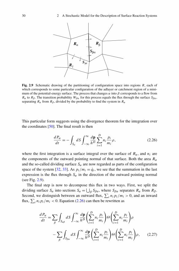
30 2 A Stochastic Model for the Description of Surface Reaction Systems

Fig. 2.9 Schematic drawing of the partitioning of configuration space into regions R, each ofwhich corresponds to some particular configuration of the adlayer or catchment region of a mini-mum of the potential-energy surface. The process that changes α into β corresponds to a flow fromRα to Rβ . The transition probability Wβα for this process equals the flux through the surface Sβα ,separating Rα from Rβ , divided by the probability to find the system in Rα

This particular form suggests using the divergence theorem for the integration overthe coordinates [50]. The final result is then

dPα

dt= −

∫

Sα

dS

∫ ∞

−∞dphD

D∑

i=1

ni

pi

mi

ρ, (2.26)

where the first integration is a surface integral over the surface of Rα , and ni arethe components of the outward pointing normal of that surface. Both the area Rα

and the so-called dividing surface Sα are now regarded as parts of the configurationspace of the system [32, 33]. As pi/mi = qi , we see that the summation in the lastexpression is the flux through Sα in the direction of the outward pointing normal(see Fig. 2.9).

The final step is now to decompose this flux in two ways. First, we split thedividing surface Sα into sections Sα =⋃β Sβα , where Sβα separates Rα from Rβ .Second, we distinguish between an outward flux,

∑i nipi/mi > 0, and an inward

flux,∑

i nipi/mi < 0. Equation (2.26) can then be rewritten as

dPα

dt=∑

β

∫

Sαβ

dS

∫ ∞

−∞dphD

(D∑

i=1

ni

pi

mi

)Θ

(D∑

i=1

ni

pi

mi

)ρ

−∑

β

∫

Sβα

dS

∫ ∞

−∞dphD

(D∑

i=1

ni

pi

mi

)Θ

(D∑

i=1

ni

pi

mi

)ρ, (2.27)

2.2 The Master Equation 31

where in the first term Sαβ (= Sβα) is regarded as part of the surface of Rβ , andthe ni are components of the outward pointing normal of Rβ . The function Θ is theHeaviside step function [51]

Θ(x) ={

1, if x ≥ 0, and0, if x < 0,

(2.28)

Equation (2.27) can be cast in the form of the master equation

dPα

dt=∑

β

[WαβPβ − WβαPα], (2.29)

if we define the transition probabilities as

Wβα =∫Sβα

dS∫∞−∞ dp/hD(

∑Di=1 nipi/mi)Θ(

∑Di=1 nipi/mi)ρ

∫Rα

dq∫∞−∞ dp/hDρ

. (2.30)

The expression for the transition probabilities can be cast in a more familiar formby using a few additional assumptions. We assume that ρ can locally (i.e., in Rα andon Sβα) be approximated by a Boltzmann-distribution

ρ = N exp

[− H

kBT

], (2.31)

where T is the temperature, kB is the Boltzmann-constant, and N is a normalizingconstant. We also assume that we can define Sβα and the coordinates in such a waythat ni = 0, except for one coordinate i, called the reaction coordinate, for whichni = 1. The integral of the momentum corresponding to the reaction coordinate canthen be done and the result is

Wβα = kBT

h

Q‡

Q, (2.32)

with

Q‡ =∫

Sβα

dS

∫ ∞

−∞dp1 . . . dpi−1 dpi+1 . . . dpD

hD−1exp

[− H

kBT

], (2.33)

Q =∫

Rα

dq∫ ∞

−∞dphD

exp

[− H

kBT

]. (2.34)

We see that this is an expression that is formally identical to the TST expression forrate constants [52]. There are differences in the definition of the partition functionsQ and Q‡, but they can generally be neglected. For example, it is quite common thatthe PES has a well-defined minimum in Rα and on Sβα , and that it can be replacedby a quadratic form in the integrals above. The borders of the integrals can then beextended to infinity and the normal partition functions for vibrations are obtained.This is sometimes called harmonic TST (see Chap. 4) [53]. The dividing surfaceSβα is then chosen so that it contains the transition state of the process, which isthen also where the PES has its minimum on Sβα .

The W ’s indicate how fast the system moves from (the catchment region of) oneminimum to another. We will often call them therefore rate constants. The system

32 2 A Stochastic Model for the Description of Surface Reaction Systems

can only move from minimum α to minimum β if the catchment region of theseminima border on each other. Only in such a case we have Wβα = 0. The right-hand-side of Fig. 2.8 shows the minima of the PES as points. Two minima are connectedif their catchment regions border on each other, and the system can move from oneto the other without having to go through a third catchment region. The result is thegraph in Fig. 2.8. The vertices of the graph are the minima of the PES and the edgesindicate how the system can move from one minimum to another.

Although we have presented the partitioning of phase space based on the catch-ment regions of the PES, this is actually not required. In fact, we have not usedthis particular partitioning in the derivation up to Eq. (2.30) anywhere. One can inprinciple partition phase space in any way one likes and derive a master equation. Itis the partitioning that defines the processes that the master equation describes. Ofcourse, most partitionings lead to processes that are hard to interpret physically, butthere are variations in the partitioning above that are useful.

The dividing surface Sβα was split to distinguish fluxes in opposite directions. Ifthere is a trajectory of the system that crosses the surface and then recrosses it, theneffectively no process has occurred, but both crossings contribute to the rate con-stants of α → β and β → α. For surface reactions such a recrossing is well knownfor adsorption and leads to the definition of a sticking coefficient (see Sect. 4.4.3).The idea of VTST is to move Sβα to remove recrossings and to minimize the rateconstants [29, 32, 33, 40]. It can be shown that when we have a canonical ensem-ble, this is equivalent to locating Sβα at a maximum of the Gibbs energy along thereaction coordinate [54, 55]. The transition state need then not be on Sβα . The tran-sition state need then generally not be on Sβα . As our derivation is a generalizationof VTST, it has the same limitations and possible ways to deal with them. We referto Chap. 4 of [40] for a fuller discussion.

2.2.3 The Master Equation for Lattice-Gas Models

In the derivation of the master equation above the subscripts α and β refer to min-ima of the PES. We want however a master equation with subscripts referring toconfigurations. We have already stated that using configurations to derive the mas-ter equation gives the same result, but there are some subtleties. So we take a closerlook at how minima of the PES and configurations relate to each other. As the co-ordinates of all atoms have well-defined values for a minimum of a PES, we alsoknow which adsorbate is at each site: i.e., we know the corresponding configuration.So it is easy to go from the minima of the PES to the configurations. The reverse isnot true in general.

The first problem is that not all configurations need to correspond to a minimumof the PES. For example, suppose that we have an adsorbate that is so large that thereis a very high repulsion when another adsorbate is at a neighboring site. A config-uration with two adsorbates at such relative positions may then not correspond to aminimum. The forces between them may push them farther apart and to other sites.

2.2 The Master Equation 33

This however does not prevent us from identifying the subscripts in the master equa-tion with configurations. We only need to make sure that the rate constant Wαβ forthe process β → α equals zero when the configuration α can not be identified witha minimum of the PES.

The other problem is that there may be more than one minimum of the PESthat leads to the same configuration. This is the case when an adsorbate has differ-ent (meta)stable structures or adsorption modes. For example, an NO molecule onRh(100) may be adsorbed perpendicular to the surface with the N end down or itmay be adsorbed parallel to the surface [56, 57]. In this case we have a choice. Wemay regard the different geometries as different adsorbates. This solves the problem,because we then do get a 1-to-1 correspondence between configurations and min-ima of the PES. Alternatively we may ignore these differences in geometry. We candeal with this by redefining the areas Rα in the partitioning of configuration space.Instead of the catchment region of one minimum, we define them as the union ofthe catchment regions of all the minima leading to the same configuration. We canalso first regard the different geometries as different adsorbates as before and thendo a coarse-graining as explained in Sect. 8.2. The result is the same. The advan-tage of disregarding these differences is that it leads to a simpler model and fasterkMC simulations. We need to point out however that disregarding the difference ingeometry may constitute an approximation that needs to be justified.

Now that we have established that the master equation can be regarded in termsof configurations of lattice-gas models, we can discuss the advantage this gives us.The number of rate constants Wαβ is enormous even if we use only a small model.Suppose that we do a simulation with a modest 100 × 100 lattice. Also supposethat we have only one type of adsorbate so that each site can either be occupiedor vacant. This gives us 2100×100 different configurations and 22×100×100 ≈ 106000

rate constants Wαβ . In general, if we have a number of sites S and each site can beoccupied in A ways then the number of configurations equals AS and the number ofrate constants is A2S . A lattice model allows us to reduce this number by the sameorder of magnitude, because what matters is only the number of different non-zerovalues that the rate constants can have.

First we note that Wαβ = 0 unless the change β → α corresponds to an actualphysical or chemical process like a reaction or diffusion of an adsorbate. This meansthat for a configuration β the number of configurations α with values Wαβ = 0 doesnot equal the number of possible configurations, but only the number of processesthat can actually take place in β . This number is only proportional to the numberof sites, and not to an exponential function of the number of sites. So the numberof rate constants is thereby reduced to cSAS with c a constant depending on thenumber of types of process but not on S.

This is still a huge number of values for the rate constants. Using translationalsymmetry only reduces this number by a factor S. Point-group symmetry only re-duces it by a factor of the order of unity. To reduce it to a workable number of rateconstants, we need to make some assumptions. Fortunately, such assumptions arealmost always valid and easy to find. The reason why the number of values for therate constants depends exponentially on the number of sites is that so far we have

34 2 A Stochastic Model for the Description of Surface Reaction Systems

assumed that the occupation of each and every site in the system can affect thesevalues. This will often be unlikely however. If we have a process involving one siteor a pair of neighboring sites, then the occupation of a site well away from this siteor these sites will not be relevant. The extreme case is where we only need to lookat the sites that change occupation, and which define the process, to determine therate constant. This means that we have just one value for a desorption of a particularadsorbate, one value for the reaction of two adsorbates, et cetera. Adsorbates that donot desorb, react, et cetera do not affect the value of the rate constant. In such a casethe number of different values of the rate constants reduces to c, the proportionalityconstant introduced above. A large majority of kMC simulations done so far haveassumed that this case is valid.

Suppose that the occupation of Senv sites in the environment of a process doesnot change but does affect the value of the rate constant because of interactionswith the adsorbates that change in the process. These interactions are called lateralinteractions. The number of values of the rate constants is then cASenv . This numberneed not be large. Suppose we look at CO desorption from a Rh(100) surface. Atlow coverage we can model this with a square lattice representing the top sites whichCO prefers [10]. We also assume that only interactions between CO molecules atnearest-neighbor positions need to be included. We then have A = 2. For desorptionwe have Senv = 4 so that there are at most 24 = 16 possibly different values for therate constants for desorption. For diffusion modeled as a CO hopping from one siteto a neighboring one we have Senv = 6 and 26 = 64 possibly different values. Wecan use point-group symmetry to reduce the number of values further.

This example shows that there are situations in which the number of values ofrate constants is relatively small even with lateral interactions, but the exponentialdependence on Senv will often necessitate another approach. We want to reduce thenumber of values for the rate constants, because these values are generally hard todetermine as will be shown in Chap. 4. For a lattice-gas model it is often possible tosplit the effect of the lateral interactions from the determination of a rate constantswithout lateral interactions. The determination of rate constants even without lateralinteractions is difficult, but need only be done for a few processes. The determinationof lateral interactions is also difficult, but here too often only few values need to bedetermined. It is the large number of combinations of lateral interactions that leadsto a very large number of possible values for rate constants with lateral interactions.These combinations can however often be determined quite easily. This is shownexplicitly in Chap. 4 and in particular Sect. 4.5. However, the number of values ofthe rate constants does also determine which kMC algorithm is the most efficient.If the number of values is small, faster algorithms can be used than when we have alarge number of values of the rate constants even if these values can be determinedeasily and fast. See Chap. 3.

To summarize. The reason why kMC simulations of surface reactions can bedone much more efficiently than simulations of systems without translational sym-metry has to do with the number of rate constants. For surface reactions this numberis either very limited when there are no lateral interactions, or can often be com-puted easily from a limited set of parameters when there are lateral interactions. In

References 35

both cases only a relatively small number of values need to be determined, althoughthey require costly calculations or time-consuming experiments (see Chap. 4). Thiscan however be done before and separately from the kMC simulations. This is notthe case for simulations of other systems.

References

1. M.P. Allen, D.J. Tildesley, Computer Simulation of Liquids (Clarendon, Oxford, 1987)2. D. Frenkel, B. Smit, Understanding Molecular Simulation: From Algorithms to Applications

(Academic Press, London, 2001)3. D.C. Rapaport, The Art of Molecular Dynamics Simulation (Cambridge University Press,

Cambridge, 2004)4. A. Zangwill, Physics at Surfaces (Cambridge University Press, Cambridge, 1988)5. J.M. Thomas, W.J. Thomas, Principles and Practice of Heterogeneous Catalysis (VCH, Wein-

heim, 1997)6. N.W. Ashcroft, N.D. Mermin, Solid State Physics (Holt, Rinehart & Winston, New York,

1976)7. A.M. de Jong, J.W. Niemantsverdriet, J. Chem. Phys. 101, 10126 (1994)8. R. Kose, W.A. Brown, D.A. King, J. Phys. Chem. B 103, 8722 (1999)9. M.J.P. Hopstaken, J.W. Niemantsverdriet, J. Chem. Phys. 113, 5457 (2000)

10. M.M.M. Jansen, C.G.M. Hermse, A.P.J. Jansen, Phys. Chem. Chem. Phys. 12, 8053 (2010)11. C.T. Kao, G.S. Blackman, M.A.V. Hove, G.A. Somorjai, C.M. Chan, Surf. Sci. 224, 77 (1989)12. M. van Hardeveld, Elementary reactions in the catalytic reduction of NO on rhodium surfaces.

Ph.D. thesis, Eindhoven University of Technology, Eindhoven (1997)13. N.V. Petrova, I.N. Yakovkin, Surf. Sci. 519, 90 (2002)14. S. Dahl, A. Logadottir, R.C. Egeberg, J.H. Larsen, I. Chorkendorff, E. Törnqvist, J.K.

Nørskov, Phys. Rev. Lett. 83, 1814 (1999)15. B. Hammer, Phys. Rev. Lett. 83, 3681 (2000)16. M.T.M. Koper, J.J. Lukkien, A.P.J. Jansen, R.A. van Santen, J. Phys. Chem. B 103, 5522

(1999)17. R. Imbihl, G. Ertl, Chem. Rev. 95, 697 (1995)18. M.M. Slin’ko, N.I. Jaeger, Oscillating Heterogeneous Catalytic Systems. Studies in Surface

Science and Catalysis, vol. 86 (Elsevier, Amsterdam, 1994)19. R.J. Gelten, A.P.J. Jansen, R.A. van Santen, J.J. Lukkien, J.P.L. Segers, P.A.J. Hilbers,

J. Chem. Phys. 108, 5921 (1998)20. V.N. Kuzovkov, O. Kortlüke, W. von Niessen, Phys. Rev. Lett. 83, 1636 (1999)21. O. Kortlüke, V.N. Kuzovkov, W. von Niessen, Phys. Rev. Lett. 83, 3089 (1999)22. M. Gruyters, T. Ali, D.A. King, Chem. Phys. Lett. 232, 1 (1995)23. M. Gruyters, T. Ali, D.A. King, J. Phys. Chem. 100, 14417 (1996)24. R. Salazar, A.P.J. Jansen, V.N. Kuzovkov, Phys. Rev. E 69, 031604 (2004)25. A.R. Leach, Molecular Modelling. Principles and Applications (Longman, Singapore, 1996)26. N.G. van Kampen, Stochastic Processes in Physics and Chemistry (North-Holland, Amster-

dam, 1981)27. J.R. Norris, Markov Chains (Cambridge University Press, Cambridge, 1998)28. D.E. Knuth, The Art of Computer Programming, Volume I: Fundamental Algorithms

(Addison-Wesley, Reading, 1973)29. J.C. Keck, J. Chem. Phys. 32, 1035 (1960)30. J.C. Keck, Discuss. Faraday Soc. 33, 173 (1962)31. J.C. Keck, Adv. Chem. Phys. 13, 85 (1967)32. P. Pechukas, in Dynamics of Molecular Collisions, Part B, ed. by W. Miller (Plenum, New

York, 1976), pp. 269–322

36 2 A Stochastic Model for the Description of Surface Reaction Systems

33. D.G. Truhlar, A.D. Isaacson, B.C. Garrett, in Theory of Chemical Reaction Dynamics, Part IV,ed. by M. Baer (CRC Press, Boca Raton, 1985), pp. 65–138

34. W.H. Miller, J. Chem. Phys. 61, 1823 (1974)35. W.H. Miller, J. Chem. Phys. 62, 1899 (1975)36. G.A. Voth, J. Phys. Chem. 97, 8365 (1993)37. V.A. Benderskii, D.E. Makarov, C.A. Wight, Adv. Chem. Phys. 88, 1 (1994)38. R.S. Berry, R. Breitengraser-Kunz, Phys. Rev. Lett. 74, 3951 (1995)39. R.E. Kunz, R.S. Berry, J. Chem. Phys. 103, 1904 (1995)40. K.J. Laidler, Chemical Kinetics (Harper & Row, New York, 1987)41. A.P.J. Jansen, Comput. Phys. Comm. 86, 1 (1995)42. R.J. Gelten, R.A. van Santen, A.P.J. Jansen, in Molecular Dynamics: From Classical to Quan-

tum Methods, ed. by P.B. Balbuena, J.M. Seminario (Elsevier, Amsterdam, 1999), pp. 737–784

43. A.P.J. Jansen, An introduction to Monte Carlo simulations of surface reactions.http://arxiv.org/abs/cond-mat/0303028 (2003)

44. I. Prigogine, Introduction to Thermodynamics of Irreversible Processes (Interscience, NewYork, 1968)

45. C. van Vliet, Equilibrium and Non-equilibrium Statistical Mechanics (World Scientific, Sin-gapore, 2008)

46. P.G. Mezey, Potential Energy Hypersurfaces (Elsevier, Amsterdam, 1987)47. D.A. McQuarrie, Statistical Mechanics (Harper, New York, 1976)48. R. Becker, Theorie der Wärme (Springer, Berlin, 1985)49. A.P.J. Jansen, J. Chem. Phys. 94, 8444 (1991)50. E. Kreyszig, Advanced Engineering Mathematics (Wiley, New York, 1993)51. A.H. Zemanian, Distribution Theory and Transform Analysis (Dover, New York, 1987)52. R.A. van Santen, J.W. Niemantsverdriet, Chemical Kinetics and Catalysis (Plenum, New York,

1995)53. G. Henkelman, G. Jóhannesson, H. Jónsson, in Progress in Theoretical Chemistry and

Physics, ed. by S.D. Schwarts (Kluwer Academic, London, 2000)54. B.C. Garrett, D.G. Truhlar, J. Am. Chem. Soc. 101, 5207 (1979)55. B.C. Garrett, D.G. Truhlar, J. Am. Chem. Soc. 102, 2559 (1980)56. A.P. van Bavel, Understanding and quantifying interactions between adsorbates: CO, NO, and

N- and O-atoms on Rh(100). Ph.D. thesis, Eindhoven University of Technology, Eindhoven(2005)

57. C. Popa, A.P. van Bavel, R.A. van Santen, C.F.J. Flipse, A.P.J. Jansen, Surf. Sci. 602, 2189(2008)

Chapter 3Kinetic Monte Carlo Algorithms

Abstract Kinetic Monte Carlo generates a sequence of configurations and timeswhen the transitions between these configurations occur. This solves the masterequation in the sense that a configuration α is obtained at time t with a probabil-ity Pα(t) that is a solution of the master equation. There are many algorithms thatyield such a sequence of configurations and which are statistically equivalent. Theyall need to determine repeatedly the time that the next process will occur, the typeof process that will occur, and the position on the surface where the process will oc-cur. Each of these can be determined in a number of ways, which can be combinedin even more ways. This results in many algorithms. Few of them are however ef-ficient. We discuss in detail the Variable Step Size Method, the Random SelectionMethod, and the First Reaction Method. We use the Variable Step Size Method toshow how to handle lists of processes, different ways to make selections of pro-cesses and process types, and how computer time and memory scales with systemsize. Time-dependent rate constants are discusses separately as the determinationof when processes take place pose special problems. Parallelization is discussedas well as some older algorithms. Some guidelines are given of how to choose analgorithm for a simulation.

3.1 Introduction

Deriving analytical results from the master equation is not possible for most systemsof interest. Approximations can be used, but they may not be satisfactory. In suchcases one can resort to kinetic Monte Carlo (kMC) simulations.

Monte Carlo methods have been known already for several decades for the mas-ter equation [1]. Following Gillespie they have become quite popular to simulatereactions in solutions [2–4]. A configuration α in that case is defined as a set{N1,N2, . . .} where Ni is the number of molecules of type i in the solution. Thereis no specification of where the molecules are, as in our case for surface reactions.In fact, the method is generally used to solve rate equations for chemical reactions.When simulating reactions one talks about Dynamic Monte Carlo (DMC) simula-tions, a term that we will use as well, or more recently Stochastic Simulation Al-gorithm (SSA) [5–7]. Many of the algorithms developed in that area can be usedfor surface reactions as well. However, the efficiency of the various algorithms (i.e.,

A.P.J. Jansen, An Introduction to Kinetic Monte Carlo Simulations of SurfaceReactions, Lecture Notes in Physics 856,DOI 10.1007/978-3-642-29488-4_3, © Springer-Verlag Berlin Heidelberg 2012

37

38 3 Kinetic Monte Carlo Algorithms

the computer time and memory) can be different. There are also tricks to increasethe efficiency of simulations of reactions in solutions that do not work for surfacereactions and vice versa [8–10].

This chapter starts with a discussion of the most widely used algorithm, whichwe call the Variable Step Size Method (see Sect. 3.2). Several aspects of the algo-rithm are improved in Sect. 3.3. These improvements are put in a broader contextas they can also be used in other algorithms. Sections 3.4 and 3.5 discuss two otheralgorithms that have been shown to be very useful. Section 3.6 extends the discus-sion to include situations in which rate constants vary in time. Section 3.7 discussesother approaches for surface reactions and Sect. 3.8 parallel algorithms. Section 3.9presents a pragmatic approach to the question of which algorithm to use, and dis-cusses other practical aspects of implementing and doing kMC simulations.

3.2 The Variable Step Size Method

The Variable Step Size Method (VSSM) method is probably the most widely usedalgorithm for kMC simulations. In fact, sometimes the name kMC is specificallyused to denote this method. We will not do this. The algorithms in this sectionand those of Sects. 3.4 and 3.5 give the same results, so we prefer to include allalgorithms that solve the master equation in kMC. VSSM is also often called the n-fold way [11]. This refers to the algorithm developed by Bortz, Kalos, and Lebowitzwhich is indeed equivalent to VSSM, but was originally developed for equilibriumMonte Carlo [12]. The name VSSM was coined by Gillespie, and was developedfor DMC [2, 3].

3.2.1 The Integral Form of the Master Equation

To start with the derivation of the kMC algorithms for the master equation it isconvenient to cast the master equation in an integral form. First we simplify thenotation of the master equation. We define a matrix W by

Wαβ = Wαβ, (3.1)

which has vanishing diagonal elements, because Wαα = 0 by definition, and a diag-onal matrix R by

Rαβ ={

0, if α = β,∑γ Wγβ, if α = β. (3.2)

If we put the probabilities of the configurations Pα in a vector P, we can write themaster equation as

dPdt

= −(R − W)P. (3.3)

3.2 The Variable Step Size Method 39

This equation can be interpreted as a time-dependent Schrödinger-equation in imag-inary time with Hamiltonian R − W. This interpretation can be very fruitful [13],and leads, among other things, to the integral form we present here.

We do not want to be distracted by technicalities at this point, so we assume thatR and W are time independent. We also introduce a matrix Q, which is defined by

Q(t) = exp[−Rt]. (3.4)

We can rewrite the master equation with this definition in the integral form

P(t) = Q(t)P(0) +∫ t

0dt ′Q

(t − t ′

)WP

(t ′), (3.5)

as can be seen by substitution of this expression in Eq. (3.3). The equation is arecurrence relation implicit in P. By substitution of the right-hand-side for P(t ′)again and again we get

P(t) =[

Q(t) +∫ t

0dt ′Q

(t − t ′

)WQ

(t ′)

+∫ t

0dt ′∫ t ′

0dt ′′Q

(t − t ′

)WQ

(t ′ − t ′′

)WQ

(t ′′)+ . . .

]P(0). (3.6)

This equation is valid also for other definitions of R and W, but the definition wehave chosen leads to a useful interpretation. Suppose at t = 0 the system is in con-figuration α with probability Pα(0). The probability that at time t the system is stillin α (i.e., no process has occurred that would change the configuration) is given byQαα(t)Pα(0) = exp(−Rααt)Pα(0). This shows that the first term in Eq. (3.6) rep-resents the contribution to the probabilities if no process occurs up to time t . Thematrix W determines how the probabilities change when some process occurs. Thesecond term of Eq. (3.6) therefore represents the contribution to the probabilities ifno process occurs between times 0 and t ′, some process occurs at time t ′, and thenno process occurs between times t ′ and t . So the second term stands for the contribu-tion to the probabilities if a single process occurs between times 0 and t . Subsequentterms represent contributions if two, three, four, et cetera processes occur. (Note thatwe use the term process for any change of the configuration. This includes chemi-cal reactions, but also for example diffusional hops of adsorbates from one site to aneighboring one. In Chaps. 5, 6, and 7 we will encounter also other processes.)

3.2.2 The Concept of the Variable Step Size Method

The idea of kMC is not to compute probabilities Pα(t) explicitly, but to start withsome particular configuration, representative for the initial state of the experimentone wants to simulate, and then generate a sequence of other configurations with thecorrect probability. The integral form gives us directly a useful algorithm to generatesubsequent configurations and the times when the configuration changes. At thesetimes some process (e.g., a chemical reaction) occurs.

40 3 Kinetic Monte Carlo Algorithms

Let’s call the initial configuration α, and let’s set the initial time to t = 0. Thenthe probability that the system is still in α at a later time t is given by

Qαα(t) = exp[−Rααt]. (3.7)

The probability distribution that the first process occurs at time t is minus the deriva-tive with respect to time of this expression: i.e.,

Rαα exp[−Rααt]. (3.8)

This can be seen by taking the integral of this expression from 0 to t , which yieldsthe probability that some process has occurred in this interval, which equals 1 −Qαα(t). We now make an important step. We move from a probability distributionfor the time that the first process may occur to a time t ′ when the first processactually occurs. This can be done by equating the probability that the system is stillin α at a later time t to a uniform deviate on the unit interval: i.e., by solving

exp[−Rααt ′

]= r, (3.9)

for t ′ where r is the uniform deviate on the unit interval [14].At time t ′ some process occurs. According to Eq. (3.6) the different processes

that transform configuration α to another configuration α′ have rate constants Wα′α .This means that the probability that the system will be in configuration α′ at timet ′ + dt is Wα′α dt , where dt is some small time interval. We therefore generate anew configuration α′ by choosing one of all possible new configurations α′ with aprobability proportional to Wα′α . This gives us a new configuration α′ at time t ′. Atthis point we’re in the same situation as when we started the simulation, and we canproceed by repeating the previous steps. So we generate a new time t ′′, using

exp[−Rα′α′

(t ′′ − t ′

)]= r, (3.10)

for the time of the new process, and a new configuration α′′ with a probability pro-portional to Wα′′α′ . Here r is again a uniform deviate on the unit interval, but notthe same one of course as in Eq. (3.9). In this manner we continue until some presetcondition is met that signals the end of the simulation.

We call this whole procedure the Variable Step Size Method (VSSM). It’s a sim-ple method that can be made very efficient. The algorithm is as follows.

Variable Step Size Method: concept (VSSMc)

1. Initialize

Generate an initial configuration α.Set the time t to some initial value.Choose conditions when to stop the simulation.

2. Time

Generate a time interval Δt when no process occurs

Δt = − 1∑β Wβα

ln r, (3.11)

where r is a uniform deviate on the unit interval.Change time to t → t + Δt .

3.2 The Variable Step Size Method 41

3. Process

Change the configuration to α′ with probability Wα′α/∑

β Wβα : i.e., do theprocess α → α′.

4. Continuation

If the stop conditions are fulfilled then stop. If not repeat at step 2.

Equation (3.11) is obtained from Eqs. (3.9) or (3.10) if we solve them for the time.We see that the algorithm yields an ordered set of configurations and times when

processes occur that can be written as

(α0, t0)t1→ α1

t2→ α2t3→ α3

t4→ . . . (3.12)

Here α0 is the initial configuration and t0 is the time at the beginning of the simula-tions. The changes αn−1 → αn are caused by processes occurring at times tn. Theseprocesses that actually occur are often called events. We will see that all algorithmsin this section and in Sects. 3.4 and 3.5 also give such a result (3.12). They are allequivalent because all give at time t a configuration α with probability Pα(t) whichis the solution of the master equation with boundary condition Pα(t0) = δαα0 witht0 the time at the beginning of the simulation.

3.2.3 Enabled and Disabled Processes

Although the algorithms in this section and in Sects. 3.4 and 3.5 yield the sameresult, they often do so at very different computational costs. We are very interestedin how computer time and memory scale with system size. It is clear that in generalthe number of processes in a system is proportional to the size of the system and alsoto the length of the simulation in real time. The computational costs will thereforescale at least linear with system size and simulation length. We will therefore focusnot on costs for a whole simulation, but instead on costs per process.

Looking at the VSSMc algorithm above, we see that it scales in the worse possi-ble way with system size. In step 2, for example, we have to sum over all possibleconfigurations. For a simple lattice with S sites and each lattice point having N

possible labels we have a total number of configurations equal to NS . This meansthat VSSMc scales exponentially with system size. Fortunately, it is easy to improvethis. Most of the terms in the summation are zero because there is no process thatchanges α into β and hence Wβα = 0. So we should only use those changes thatcan actually occur: i.e., we should keep track of the possible processes. Processesthat can actually occur at a certain location we call enabled. The total number of(enabled) processes is proportional to the system size, so we can reduce the scalingof computer time per process so that it is not worse than proportional to the systemsize. Actually, we can reduce the costs even further because we need not determineall enabled processes every time at steps 2 and 3. A process generally has only alocal effect and does not affect processes far away. If a process occurs, this causes a

42 3 Kinetic Monte Carlo Algorithms

Fig. 3.1 The left drawing shows part of a configuration for a model of CO oxidation. The fatCO and oxygen form CO2 which is removed from the surface. The middle drawing shows newlyenabled processes: CO can adsorb at the sites marked by dark gray circles, oxygen can adsorbdissociatively on neighboring sites indicated by two light gray circles on the line connecting thesites. The right drawing indicates a disabled process: the two encircled sites had a CO and anoxygen that could form a CO2

local change in the configuration. This change makes new processes possible onlylocally, whereas other processes are not possible anymore also locally. We say thatsuch latter processes become disabled. The number of newly enabled and disabledprocesses only depends on what the configuration looks like at the location where aprocess has just occurred, but it does not depend on the system size (see Fig. 3.1). Soinstead of determining all enabled processes again and again we do this only at theinitialization and then update a list of all enabled processes. Such a list is sometimescalled an event list. The algorithms then becomes as follows.

Variable Step Size Method: improved version (VSSMi)

1. Initialize

Generate an initial configuration α.Make a list Lproc of all processes.Calculate kα =∑β Wβα , with the sum being done only over the processes inLproc.Set the time t to some initial value.Choose conditions when to stop the simulation.

2. Time

Generate a time interval Δt when no process occurs

Δt = − 1

kα

ln r, (3.13)

where r is a uniform deviate on the unit interval.Change time to t → t + Δt .

3. Process

Choose the process α → α′ from Lproc with probability Wα′α/kα : i.e., do theprocess α → α′.

4. Update

3.3 Some General Techniques 43

Remove the process α → α′ from Lproc.Add new enabled processes to Lproc and remove disabled processes.Use these changes to Lproc to calculate kα′ from kα .

5. Continuation

If the stop conditions are fulfilled then stop. If not repeat at step 2.

The reasoning leading to VSSMi suggests that the computer time per process ofthis algorithm does not depend on system size. However, that is still not true. Thereare two problems. First, choosing the process in step 3 can in general not be done inconstant time just with the list of all processes as we will see in Sect. 3.3.1. Second,adding new enabled processes to the list of processes can be done easily in constanttime, but removing disabled processes presents a problem. One can scan the list ofall processes and remove all disabled processes from the list, but that is an operationproportional to the system size.

3.3 Some General Techniques

There are a number of concepts and techniques that are useful to improve VSSMi,but that can also be used to speed up the other algorithms that we will discuss.This is because all algorithms essentially have to do the same thing. They have todetermine repeatedly which process occurs, when it occurs, and where it occurs. Wewill introduce in this section hierarchical selection, using disabled processes, andoversampling. We will also show explicitly how to use these techniques in VSSM.Other algorithms using these techniques will be discussed in subsequent sections.

3.3.1 Selection Methods

Step 3 of VSSMi (Sect. 3.2.3) is a selection. Because different processes have dif-ferent probabilities of being selected it is called a weighted selection. To make thisselection one has to define cumulative rate constants Cα′α =∑β≤α′ Wβα . The pro-cesses in Lproc need to be ordered. In principle, it does not matter what criterionis used for the ordering. A simple and convenient one is to order the processes ac-cording to the order in which the processes are generated in steps 1 and 4 of theVSSMi algorithm. The summation is over all processes α → β preceding α → α′(β < α′) and α → α′ itself. The process α → α′ can then be picked by choosingα′ using Cα′−1,α < rkα ≤ Cα′α where r is a uniform deviate on the unit intervaland α → α′ − 1 is the process before α → α′ in the ordering of the processes. Thisweighted selection scales linearly with the number of processes and the system size.The reason for this is that we have to scan all the cumulative rate constants Cα′α .

It is often possible to choose a process in constant time. To accomplish this wesplit the list of all processes in groups containing processes of the same type (or

44 3 Kinetic Monte Carlo Algorithms

Fig. 3.2 For a weighted selection the lengths of the bars in the top part of the figure have to beadded. If all bars have the same length then we can simply choose a bar at random. This is uniformselection. The bottom part shows how selection can be done with a binary tree. You store partialsums of subtrees in the nodes, which makes traversing the tree easier. The middle part shows aform of selection using oversampling (see Sect. 3.3.4). All bars have a length smaller or equalto M . A bar is chosen randomly (uniform selection) and then accepted with probability Wn/M

more general with the same rate constant). Two processes are of the same type ifthey differ only in their position and/or orientation. So CO adsorption, NO disso-ciation (NO → N + O) and N2 associative desorption (2N → N2) are examplesof process types. If L

(i)proc is the list of N(i) processes with rate constant W(i),

then we proceed as follows. First, we pick a type of process j with probabilityN(j)W(j)/

∑i N

(i)W(i), and then we pick from L(j)proc a process at random. The first

part scales linearly with the number of lists, because it is a weighted selection. Thisnumber does not depend on the system size, however, but only on the number ofprocess types or the number of rate constants. The second part is a uniform selec-tion, which means that each process has the same probability of being chosen. Thiscan be done in constant time. So the second part also does not depend on the systemsize. If the number of process types is small, and it often is, this method is veryefficient (see Fig. 3.2). Selecting first the process type and then a specific process ofthe type is a hierarchical selection.

It is possible to do the weighted selection of the processes also in a time propor-tional to the logarithm of the system size by using a binary tree or priority queueas shown in the bottom part of Fig. 3.2 [15]. Each node of the tree has a process,its rate constant, and the cumulative rate constants of all processes of the node andboth branches below the node. After rkα has been calculated we look for the nodewith Cleft < rkα ≤ Cleft + Wnode where Wnode is the rate constant of the process ofthe node and Cleft is the cumulative rate constant of the top node of the left branch.

3.3 Some General Techniques 45

If there is no left branch then we define Cleft = 0. To find the node we do the fol-lowing.

1. Start

Set X = rkα .Take the top node of the tree.

2. Process found?

if Cleft < X ≤ Cleft + Wnodethen stop: take the process of the nodeelse go to the next step

3. Continue in the left branch?

if X ≤ Cleftthen take the top node of the left branch and continue at step 2else go to the next step

4. Continue in the right branch.

Set X → X − (Cleft + Wnode).Take the top node of the right branch and continue at step 2.

The number of nodes we have to inspect is equal to the depth of the tree. If thetree is well-balanced with all subtrees below a level of approximately equal depththis is proportional to the logarithm of the system size. We can use this method alsofor a weighted selection of the process type, if the number of process types is large.In fact this occurs in DMC simulations of reactions in solutions and the method wedescribe here is one method that is used for these simulations [4].

Of the three selection methods described above, uniform selection is clearly thefastest. The drawback is of course that it can only rarely be used, because all prob-abilities must be the same. If the selection has to be made from a large number ofprocesses, then using a binary tree is more efficient than weighted selection, becauseit scales better with the number of processes. However, if the number of processesis small, than a weighted selection is faster. There is more overhead in setting up abinary tree and updating the information in the nodes. This overhead determines theefficiency if the number of processes becomes too small. Hierarchical selection is away to use the advantage of uniform selection as much as possible even when theprobabilities are not the same.

Because uniform selection is so efficient, another variation might even be usedif the probabilities are not the same but still similar. Suppose M ≥ Wβα for allprocesses α → β . First use a uniform selection to choose a process randomly, sayγ → γ ′. Next accept that process with probability Wγ ′γ /M . If the process is notaccepted, then repeat the procedure until a process has been accepted. Accepting aprocess with a probability less than one is a form of oversampling (see Sect. 3.3.4).This variation of uniform selection is efficient provided a process is accepted beforetoo many uniform selections have occurred: i.e., the average of Wβα/M should not

46 3 Kinetic Monte Carlo Algorithms

be too small. We will see later that in this form of selection it is not always necessaryto know Wβα/M explicitly (see Sects. 3.3.3 and 3.4).

We will see that grouping all processes with the same rate constant in a processtype is not efficient if there are many different rate constants, because each list L

(i)proc

will then have one few processes and choosing a process type is little different fromchoosing a process directly. The following procedure by Schulze may then help[16, 17]. Define a series of ordered rate constants M(i) with M(i) < M(j) if andonly if i < j . Make lists L(i) with processes. Put process α → β in list L(i) ifM(i−1) < Wβα ≤ M(i). To select a process first select a list L(i) with probabilityN(i)L(i)/

∑j N(j)L(j) with N(i) the number of processes in L(i). Next select a

process α → β from L(i) uniformly but accept it with probability Wβα/M(i). Theprocedure is the same as the one for process types except that in the last step uniformselection has been replaced by uniform selection with oversampling. This allows usto restrict the number of list even if there are many rate constants.

3.3.2 Using Disabled Processes

The problem of removing disabled processes mentioned at the end of Sect. 3.2.3has a surprisingly simple solution, although it is a bit more difficult to see that it isactually correct. Instead of removing the disabled processes, we simply leave themin the list of all processes, but when a process has to occur we check if it is disabled.If it is, we remove it. If it is an enabled process, we treat it as usual. That this iscorrect can be proven as follows. Suppose that ken is the sum of the rate constantsof all enabled processes, and we have one disabled process with rate constant kdis.Also suppose without loss of generality that the system is at time t = 0. The prob-ability distribution for the first process to occur is ken exp(−kent) (see Eq. (3.8)).If we work with the list that includes the disabled process then the probability dis-tribution for the first process occurring at time t being also an enabled process isken exp(−(ken + kdis)t), which is the probability that no process occurs until time t

(= (ken + kdis) exp(−(ken + kdis)t)) times the probability that the process is enabled(= ken/(ken + kdis)). This is the first contribution to the probability distribution forthe enabled process if the disabled process is not removed. The probability distribu-tion that the first process is disabled but the second process is enabled and occurs attime t is given according to Eq. (3.6) by

∫ t

0dt ′[kene

−ken(t−t ′)] kdis

ken + kdis

[(ken + kdis)e

−(ken+kdis)t′]

= kene−kent kdis

∫ t

0dt ′e−kdist

′

= kene−kent

[1 − e−kdist

]. (3.14)

Adding this to ken exp(−(ken + kdis)t) gives us ken exp(−kent), which is what weshould have.

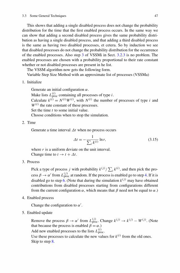
3.3 Some General Techniques 47

This shows that adding a single disabled process does not change the probabilitydistribution for the time that the first enabled process occurs. In the same way wecan show that adding a second disabled process gives the same probability distri-bution as having a single disabled process, and that adding a third disabled processis the same as having two disabled processes, et cetera. So by induction we seethat disabled processes do not change the probability distribution for the occurrenceof the enabled processes. Also step 3 of VSSMi in Sect. 3.2.3 is no problem. Theenabled processes are chosen with a probability proportional to their rate constantwhether or not disabled processes are present in he list.

The VSSM algorithm now gets the following form.Variable Step Size Method with an approximate list of processes (VSSMa)

1. Initialize

Generate an initial configuration α.Make lists L

(i)proc containing all processes of type i.

Calculate k(i) = N(i)W(i), with N(i) the number of processes of type i andW(i) the rate constant of these processes.Set the time t to some initial value.Choose conditions when to stop the simulation.

2. Time

Generate a time interval Δt when no process occurs

Δt = − 1∑i k

(i)ln r, (3.15)

where r is a uniform deviate on the unit interval.Change time to t → t + Δt .

3. Process

Pick a type of process j with probability k(j)/∑

i k(i), and then pick the pro-

cess β → α′ from L(j)proc at random. If the process is enabled go to step 4. If it is

disabled go to step 6. (Note that during the simulation k(j) may have obtainedcontributions from disabled processes starting from configurations differentfrom the current configuration α, which means that β need not be equal to α.)

4. Enabled process

Change the configuration to α′.

5. Enabled update

Remove the process β → α′ from L(j)proc. Change k(j) → k(j) − W(j). (Note

that because the process is enabled β = α.)Add new enabled processes to the lists L

(i)proc.

Use these processes to calculate the new values for k(i) from the old ones.Skip to step 8.

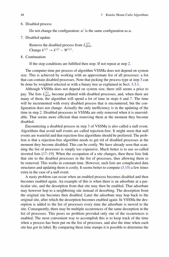
48 3 Kinetic Monte Carlo Algorithms

6. Disabled process

Do not change the configuration: α′ is the same configuration as α.

7. Disabled update

Remove the disabled process from L(j)proc.

Change k(j) → k(j) − W(j).

8. Continuation

If the stop conditions are fulfilled then stop. If not repeat at step 2.

The computer time per process of algorithm VSSMa does not depend on systemsize. This is achieved by working with an approximate list of all processes: a listthat can contain disabled processes. Note that picking the process type at step 3 canbe done by weighted selected or with a binary tree as explained in Sect. 3.3.1.

Although VSSMa does not depend on system size, there still seems a price topay. The lists L

(i)proc become polluted with disabled processes, and, when there are

many of them, the algorithm will spend a lot of time in steps 6 and 7. The timewill be incremented with every disabled process that is encountered, but the con-figuration does not change. Actually the only inefficiency is in the updating of thetime in step 2. Disabled processes in VSSMa are only removed when it is unavoid-able. That seems more efficient than removing them at the moment they becomedisabled.

Encountering a disabled process in step 3 of VSSMa is also called a null event.Algorithms that avoid null events are called rejection-free. It might seem that nullevents are wasteful and that rejection-free algorithms should be preferred. The prob-lem is that a rejection-free algorithm needs to get rid of disabled processes at themoment they become disabled. This can be costly. We have already seen that scan-ning the list of processes is simply too expensive. Much better is to use so-calledinverted lists [17–19]. When the occupation of a site changes, then these lists linkthat site to the disabled processes in the list of processes, thus allowing them tobe removed. This works in constant time. However, such lists are complicated datastructures and updating them is costly. It seems better to compute (3.15) a few timesextra in the case of a null event.

A nasty problem can occur when an enabled process becomes disabled and thenbecomes enabled again. An example of this is when there is an adsorbate at a par-ticular site, and the desorption from that site may then be enabled. That adsorbatemay however hop to a neighboring site instead of desorbing. The desorption fromthe original site becomes then disabled. Later the adsorbate may hop back to theoriginal site, after which the desorption becomes enabled again. In VSSMa the des-orption is added to the list of processes every time the adsorbate is moved to thesite. Consequently, there may be multiple occurrences of the same desorption in thelist of processes. This poses no problem provided only one of the occurrences isenabled. The most convenient way to accomplish this is to keep track of the timewhen a process has been put on the list of processes, and also the time when eachsite has got its label. By comparing these time stamps it is possible to determine the

3.3 Some General Techniques 49

last time that a process has been put in the list of processes. That process is the onlyone that should be enabled. Because of round-off errors one should not use floatingpoint representation for the time stamps. Instead on should use integers time stamps:for example, the number of processes that have occurred since the beginning of asimulation.

3.3.3 Reducing Memory Requirements

We might also want to change the VSSM algorithm, not because of time, but becauseof memory considerations. The descriptions of the algorithms so far use a list of allprocesses. This list is quite large and scales with system size. We can do away withthis list at the cost of increasing computer time, although the algorithm will still notdepend on the system size.

Instead of keeping track of all individual processes we only keep track of howmany processes there are of each different type: i.e., no lists L

(i)proc but only the num-

bers N(i). Because there are no lists we have to count how many processes becomeenabled and disabled after a process has occurred. This is similar to adding onlyenabled processes and can be done in constant time. (Note that this is only becausewe are using no lists. Searching for disabled processes in lists and then removingthem is what costs time, not counting how many processes become disabled.) Thismeans that the number N(i) will be exact. The only problem is, after the type ofprocess is determined, how to determine which particular process will occur. Thiscan be done by randomly searching on the surface. The number of places one hasto look does not depend on the system size, but on the probability that the processcan occur on a randomly selected site. This random search for the location of theprocess is a form of uniform selection with oversampling as described in Sect. 3.3.1.Another application of such a uniform selection will be given in Sect. 3.9. If the typeof process can occur on many places, then a location for a that process will be foundrapidly.

To make the formulation of the new algorithm not too difficult we use here amore restrictive definition of a process type, in the sense that two processes are ofthe same type if one can be obtained from the other by a translation. Previously wealso talked about the same process type if the orientation was different. We don’t dothis here, because we want to have an unambiguous meaning if we say that a processoccurs at a particular site (see step 4 of VSSMs) even if more sites are involved. Forexample, if we have a process type of an A reacting with a B where the B is at a siteto the right of the A, then by the site of this process we mean the site where the Ais. The new algorithm now becomes as follows.

Variable Step Size Method with random search for the location of processes(VSSMs)

1. Initialize

Generate an initial configuration.

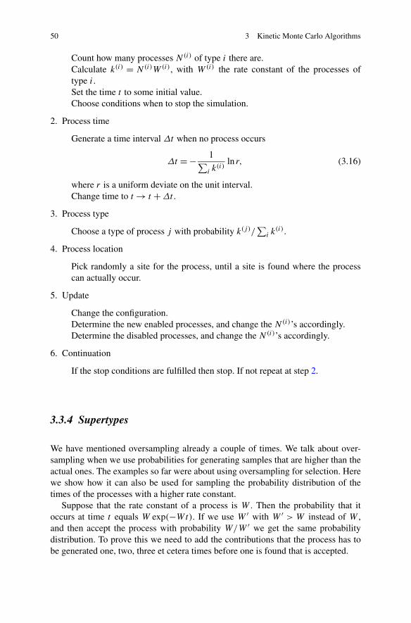
50 3 Kinetic Monte Carlo Algorithms

Count how many processes N(i) of type i there are.Calculate k(i) = N(i)W(i), with W(i) the rate constant of the processes oftype i.Set the time t to some initial value.Choose conditions when to stop the simulation.

2. Process time

Generate a time interval Δt when no process occurs

Δt = − 1∑i k

(i)ln r, (3.16)

where r is a uniform deviate on the unit interval.Change time to t → t + Δt .

3. Process type

Choose a type of process j with probability k(j)/∑

i k(i).

4. Process location

Pick randomly a site for the process, until a site is found where the processcan actually occur.

5. Update

Change the configuration.Determine the new enabled processes, and change the N(i)’s accordingly.Determine the disabled processes, and change the N(i)’s accordingly.

6. Continuation

If the stop conditions are fulfilled then stop. If not repeat at step 2.

3.3.4 Supertypes

We have mentioned oversampling already a couple of times. We talk about over-sampling when we use probabilities for generating samples that are higher than theactual ones. The examples so far were about using oversampling for selection. Herewe show how it can also be used for sampling the probability distribution of thetimes of the processes with a higher rate constant.

Suppose that the rate constant of a process is W . Then the probability that itoccurs at time t equals W exp(−Wt). If we use W ′ with W ′ > W instead of W ,and then accept the process with probability W/W ′ we get the same probabilitydistribution. To prove this we need to add the contributions that the process has tobe generated one, two, three et cetera times before one is found that is accepted.

3.4 The Random Selection Method 51

W

W ′ W′ exp

(W ′t

)

+∫ t

0dt ′ W

W ′ W′e−W ′(t−t ′)

[1 − W

W ′

]W ′e−W ′t ′

+∫ t

0dt ′∫ t ′

0dt ′′ W

W ′ W′e−W ′(t−t ′)

×[

1 − W

W ′

]W ′e−W ′(t ′−t ′′)

[1 − W

W ′

]W ′e−W ′t ′′ + . . .

= We−W ′t[

1 +[

1 − W

W ′

]W ′t + 1

2

[1 − W

W ′

]2

W ′2t2 + . . .

]

= We−W ′t e[1−W/W ′]W ′t = We−Wt . (3.17)

A useful application of this is VSSM with supertypes [20]. Suppose that the num-ber of process types is very large so that one does no longer want to do a weighted se-lection of the process type in step 3 of VSSMs (Sect. 3.3.3) or VSSMa (Sect. 3.3.2).One can of course use a binary tree, but one can also partition all process types ina small number of supertypes. We define a rate constant for each supertype as fol-lows. Suppose (j, k) is a process type k of supertype j with rate constant W(j,k). Wedefine Wj as the largest of all rate constants W(j,k). Instead of selecting a processtype directly, we first select a supertype using for example weighted selection witha probability proportional to Wj , update the time, then select a process uniformly,and finally accept it with probability W(j,k)/Wj . Note that this method can be re-garded as a variation of the method by Schulze discussed in Sect. 3.3.1. Here theWj ’s function as the M(i)’s in Schulze’s method.

Such supertypes might be very useful when we have a system with interactionsbetween the adsorbates that affect the rate constants. In that case the rate constantsdo not only depend on the process type, but also on the occupation of the sites aroundthe sites on which the process occurs. The number of these surrounding sites maybecome several dozen and each may be occupied in several ways. All possible waysthe surrounding sites can be occupied, and hence the number of rate constants, canbe enormous. In this case we can define a supertype as the process type itself, andthe corresponding rate constant as the highest possible rate constant for the processdepending on the occupation of the surrounding sites.

How efficient oversampling and the use of supertypes is depends very much onthe probability that processes are accepted. In the example with the lateral interac-tions it turns out that the interactions should not be larger than the thermal energy(see Sect. 4.5.5).

3.4 The Random Selection Method

The determination of a process and the time it occurs can be split in three parts:the time of the process, the type of the process, and the site of the process. The last

52 3 Kinetic Monte Carlo Algorithms

two parts were combined in the previous versions of VSSM. The determination ofthe process type has to be done before the determination of the location of the pro-cesses in VSSMs, as otherwise one doesn’t know when to stop searching in step 4,but the time of the process can be determined independently from which processesoccurs where. It is also possible to determine all three parts independently. This hasthe advantage that less bookkeeping is necessary: adding and removing processes toupdate lists or numbers of types of processes is not necessary. However the draw-back is the same as in VSSMs, only worse, as in step 4 of VSSMs processes willbe attempted at certain locations where the processes cannot occur. If this does notoccur too often however, then this drawback may be small.

The trick is again to use oversampling. Suppose we have just one type of processand that we have N of them. (A process type is defined here in the same way as forVSSMs. Two processes are only of the same type if they can be transformed intoeach other by a translation.) The time to the next occurrence of a process is thengiven by the probability distribution NW exp(−NWt) where W is the rate constantof the process. If we assume, however, that we have M of these processes withM > N then we can also generate the time of the next process from the distributionMW exp(−MWt), but then accept the process with probability N/M . The proof ofthis is given in Sect. 3.3.4. See Eq. (3.17) and substitute NW for W and MW forW ′.

The following algorithm is useful if we do not need to determine N explicitly.This can be accomplished if we assume that all process types can occur everywhereon the surface. In terms of lists this means that each list L

(i)proc has the same S pro-

cesses during an entire simulation. Because the lists do not change and they have asimple definition, we do not need to determine them explicitly. Also the times of theprocesses are always taken from the same probability distribution, and the probabil-ities to choose a process type do not change. The algorithm looks as follows.

Random Selection Method (RSM)

1. Initialize

Generate an initial configuration.Set the time t to some initial value.Define k = SWsum where Wsum is the sum of the rate constants W(i)’s oftype i.Choose conditions when to stop the simulation.

2. Process time

Generate a time interval Δt when no process occurs

Δt = −1

kln r, (3.18)

where r is a uniform deviate on the unit interval.

3. Process type

Choose a type of process randomly.

3.5 The First Reaction Method 53

4. Process location

Choose a site randomly.

5. Update

Change time to t → t + Δt .If the process is possible at the site from step 4, then accept the process withprobability W(i)/Wsum where i is the type of process from step 3.If the process is possible and accepted, change the configuration.

6. Continuation

If the stop conditions are fulfilled then stop. If not repeat at step 2.

This algorithm is called the Random Selection Method (RSM). Note that the timefor a process, the type of the process, and the location of the process can be donein any order. Only the time and the configuration of the system need to be updated.The method is therefore very efficient, provided that processes are accepted oftenin step 5. Also note that in the proof that this algorithm is correct we used theprobability N/M , but that this probability is never used explicitly in the algorithm.Step 5 accepts processes with this probability implicitly.

3.5 The First Reaction Method

Instead of splitting the time, the type, and the location of a process, it is also possibleto combine them. This is done in the First Reaction Method.

The First Reaction Method (FRM)

1. Initialize

Generate an initial configuration α.Set the time t to some initial value.Make a list Lproc containing all processes.Generate for each process α → β in Lproc a time of occurrence

tβα = t − 1

Wβα

ln r (3.19)

with Wβα the rate constant for the process and r a uniform deviate on the unitinterval.Choose conditions when to stop the simulation.

2. Process

Take the process α → α′ with tα′α ≤ tβα for all β .If the process is enabled go to step 3. If not go to step 4.

3. Enabled update

Change the configuration to α′.

54 3 Kinetic Monte Carlo Algorithms

Change time to t → tα′α .Remove the process α → α′ from Lproc.Add new enabled processes to Lproc and generate for each new process α′ → β

a time of occurrence

tβα′ = t − 1

Wβα′ln r. (3.20)

Skip to step 5.

4. Disabled update

Do not change the configuration: α′ is the same configuration as α.Do not change the time.Remove the disabled process from Lproc.

5. Continuation

If the stop conditions are fulfilled then stop. If not set α to α′ and repeat atstep 2.

This algorithm is also known in computer science where it is called DiscreteEvent Simulation (DES) [21]. In FRM the determination of the type and the site ofa process is replaced by comparing times of occurrences for individual processes.That this is correct can be seen as follows. Suppose we have N processes with rateconstants W1,W2, . . . ,WN . The probability that no process occurs in the interval[0, t] is then exp[−t

∑Nn=1 Wn], whereas the probability that neither process 1 nor

process 2 nor any other process occurs in that interval equals∏N

n=1 exp(−Wnt),which is obviously the same as the previous expression. This proves that FRM gen-erates correct times for processes. It’s a bit more work to show that the processesare chosen with the correct probability. The probability distributions for the times ofthe processes are Wi exp(−Wit) with i = 1,2, . . . ,N . The probability that process1 occurs before any of the other processes in the FRM algorithm is given by

∫ ∞

0dtW1e

−W1t

∫ ∞

t

dt ′W2e−W2t

′. . .

∫ ∞

t

dt ′′WNe−WNt ′′

= W1

∫ ∞

0dte−W1t e−W2t . . . e−WNt = W1

W1 + W2 + . . . + WN

. (3.21)

For process i we find Wi/(W1 + W2 + . . . + WN), which shows that FRM alsochooses the processes with the correct probability. So we see that one can eithergenerate one time for all processes and then choose one process, or generate timesfor all processes and then take the first that will occur. We will use this in Sect. 3.9in another way.

The disadvantage of FRM is the determination of the process with the smallesttime of occurrence. Scanning a list of all process for each new process scales linearlywith system size. More efficient is to make the list of all processes an ordered one,and keep it ordered during a simulation. This can for example be done with a binarytree. Getting the next process does not depend on system size, but inserting new

3.6 Time-Dependent Rate Constants 55

processes in Lproc is proportional to the logarithm of the system size [15]. This isnot as good as constant time, but it is not particularly bad either. Still VSSM is oftenmore efficient than FRM, but VSSM cannot always be used as we will show later,whereas FRM can always be used.

Note that disabled processes are not removed from the list of all processes. Notealso that we only have to generate times for the new enabled processes. Times forprocesses already in Lproc need not be generated again. Suppose that at time t = t1a time has been generated for a process with rate constant W . The probability distri-bution for that time is W exp[−W(t − t1)]. Now assume that at time t = t2 > t1 theprocess has not occurred. We might generate a new time using the new probabilitydistribution W exp[−W(t − t2)]. However, the ratio of the values of these proba-bility distributions for times t > t2 is W exp[−W(t − t2)]/W exp[−W(t − t1)] =exp[W(t2 − t1)] is a constant. Hence relative probabilities for the times t > t2 thatthe process can occur are the same for both probability distributions, and no newtime needs to be generated. Another way to look at this is that the probability thatthe process has not occurred yet at time t2 is exp[−W(t2 − t1)]. The conditionalprobability that the process will take place at time t provided it has not occurred yetat time t2 equals W exp[−W(t − t1)]/ exp[−W(t2 − t1)] = W exp[−W(t − t2)].

3.6 Time-Dependent Rate Constants

If the rate constants Wαβ are themselves time dependent, then the integral form(3.6) needs to be adapted. This situation arises, for example, when dealing withTemperature-Programmed Desorption or Reactions (TPD/TPR) [22–24], and whendealing with voltammetry [25]. The definitions of the matrices W and R remain thesame, but instead of a matrix Q(t) we get

Q(t ′, t)= exp

[−∫ t ′

t

dt ′′R(t ′′)]

. (3.22)

With this new Q matrix the integral form of the master equation becomes

P(t) =[

Q(t,0) +∫ t

0dt ′Q

(t, t ′)W(t ′)Q(t ′,0

)

+∫ t

0dt ′∫ t ′

0dt ′′Q

(t, t ′)W(t ′)Q(t ′, t ′′

)W(t ′′)Q(t ′′,0

)+ . . .

]

× P(0). (3.23)

The interpretation of this equation is the same as that of Eq. (3.6). This means thatit is also possible to use VSSM to solve the master equation. The relevant equationto determine the times of the processes becomes

Q(tn, tn−1) = r, (3.24)

where tn−1 is the time of the last process that has occurred, and the equation shouldbe solved for tn, which is the time of the next process. If just after tn−1 the system is

56 3 Kinetic Monte Carlo Algorithms

in configuration αn−1, then the next process leading to configuration αn should bechosen from all possible process with probability proportional to Wαnαn−1(tn). Notethe argument of Wαnαn−1 here.

The drawback of VSSM for time-dependent rate constants is that the equationfor the times of the processes is often very difficult to be solved efficiently. Equa-tion (3.24) can in general not be solved analytically, but a numerical solution mayalso not be easy. The problem is that R in Eq. (3.22) can contain many terms orterms from processes that have a very different time dependence. A possible solu-tion is to use VSSM for each process type separately: i.e., we solve Eq. (3.24) foreach process type separately. This avoids the problem of the different time depen-dences. The next process is then of the type with the smallest value for tn, and thefirst process is chosen from those of that type as in VSSM [20, 26]. This worksprovided the number of process types is small.

Instead of computing a time for the next process using the sum of the rate con-stants of all possible processes, we can also compute a time for each process. So ifwe’re currently at time t and in configuration α, then we compute for each processα → β a time tβα using

exp

[−∫ tβα

t

dt ′Wβα

(t ′)]= r, (3.25)

where r is again a uniform deviate on the unit interval. The first process to occuris then the one with the smallest tβα . It can be shown that this time has the sameprobability distribution as that of VSSM just as for time-independent rate constants.This method is FRM for time-dependent reaction rate constants [22].

The equations defining the times for the processes, Eq. (3.25), are often mucheasier to solve than Eq. (3.24). It may seem that this is offset by the fact that thenumber of equations (3.25) that have to be solved is very large, but that is not reallythe case. Once one has computed the time of a certain process, it is never necessaryto compute the time of that process again just as for the case of time-independentrate constants. In fact, the only difference concerning the number of times (3.24)and (3.25) has to be solved is due to there possibly still being processes in the listof processes at the end of a simulation. In FRM equation (3.25) has already beensolved for these processes, as this is done when a process becomes enabled. Thisis not necessary, and in VSSM this is not done for these processes. Apart from thisdifference the number of times Eqs. (3.24) and (3.25) have to be solved is equal tothe number of processes (enabled or disabled) that are chosen to actually change theconfiguration during a simulation: step 3 in VSSMa (Sect. 3.3.2) and step 2 of FRM(Sect. 3.5).

Equation (3.25) can have the interesting property that it may have no solution.The expression

Pnot(t) = exp

[−∫ t

tnow

dt ′Wβα

(t ′)]

(3.26)

is the probability that the process α → β has not occurred at time t if the currenttime is tnow. As Wβα is a non-negative function of time, this probability decreases

3.6 Time-Dependent Rate Constants 57

with time. It is bounded from below by zero, but it need not go to zero for t → ∞,because the integral need not diverge. If it does not, then there is no solution whenr in Eq. (3.25) is smaller than limt→∞ Pnot(t). This means that there is a finiteprobability that the process will never occur. This is the case with some process involtammetric experiments [25]. There is always a solution if the integral goes toinfinity. This is the case when Wβα goes slower to zero than 1/t , or does not go tozero at all.

How to solve Eq. (3.25) depends very much on the time dependence of the rateconstants W . The dependence for voltammetry leads to an equation that can besolved analytically fairly easily, despite the fact that for some processes there maynot be a solution. The rate constant for processes on an electrode can be written as[27, 28]

W = W0 exp

[αγ eE

kBT

](3.27)

with α the transfer coefficient (0 ≤ α ≤ 1), γ the number of electrons transferred tothe electrode when the process takes place, e the elementary charge, E the electrodepotential, and W0 the rate constant at E = 0. In voltammetry we have E = E0 + ϕt

with ϕ the sweep rate: i.e., the rate with which the electrode potential is changed.This gives us

∫ t

tnow

dt ′W0 exp

[αγ e(E0 + ϕt ′)

kBT

](3.28)

= W0kBT

αγ eE0exp

[αγ eE0

kBT

]{exp

[αγ eϕt

kBT

]− exp

[αγ eϕtnow

kBT

]}. (3.29)

We see that this is finite if γ ϕ ≤ 0 with a maximum of

−W0kBT

αγ eE0exp

[αγ e(E0 + ϕtnow)

kBT

]. (3.30)

We have to equate this to − ln r to find a solution for Eq. (3.25). If − ln r is largerthan this maximum, there is no solution. Otherwise the solution is

t = kBT

αγ eϕln

{exp

[αγ eϕtnow

kBT

]− αγ eϕ

W0kBTexp

[−αγ eE0

kBT

]ln r

}. (3.31)

For TPD there always is a solution that needs to be determined numerically, butthis can be done very efficiency. The rate constant can be written as

W = ν exp

[− Eact

kB(T0 + Bt)

](3.32)

with Eact the activation energy, ν the prefactor, T0 the temperature at time t = 0,and B the heating rate. We now get

∫ t

tnow

dt ′ν exp

[− Eact

kB(T0 + Bt ′)

]= Ω(t) − Ω(tnow) (3.33)

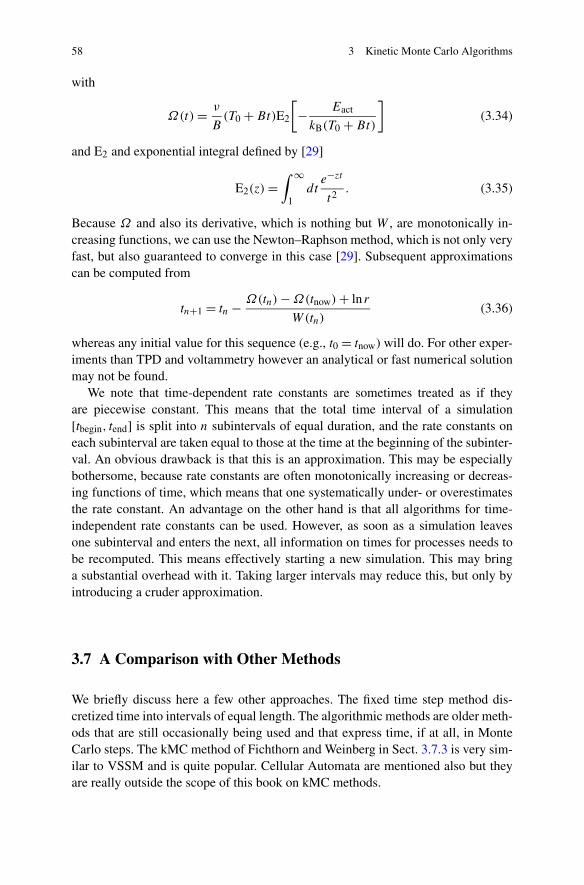
58 3 Kinetic Monte Carlo Algorithms

with

Ω(t) = ν

B(T0 + Bt)E2

[− Eact

kB(T0 + Bt)

](3.34)

and E2 and exponential integral defined by [29]

E2(z) =∫ ∞

1dt

e−zt

t2. (3.35)

Because Ω and also its derivative, which is nothing but W , are monotonically in-creasing functions, we can use the Newton–Raphson method, which is not only veryfast, but also guaranteed to converge in this case [29]. Subsequent approximationscan be computed from

tn+1 = tn − Ω(tn) − Ω(tnow) + ln r

W(tn)(3.36)

whereas any initial value for this sequence (e.g., t0 = tnow) will do. For other exper-iments than TPD and voltammetry however an analytical or fast numerical solutionmay not be found.

We note that time-dependent rate constants are sometimes treated as if theyare piecewise constant. This means that the total time interval of a simulation[tbegin, tend] is split into n subintervals of equal duration, and the rate constants oneach subinterval are taken equal to those at the time at the beginning of the subinter-val. An obvious drawback is that this is an approximation. This may be especiallybothersome, because rate constants are often monotonically increasing or decreas-ing functions of time, which means that one systematically under- or overestimatesthe rate constant. An advantage on the other hand is that all algorithms for time-independent rate constants can be used. However, as soon as a simulation leavesone subinterval and enters the next, all information on times for processes needs tobe recomputed. This means effectively starting a new simulation. This may bringa substantial overhead with it. Taking larger intervals may reduce this, but only byintroducing a cruder approximation.

3.7 A Comparison with Other Methods

We briefly discuss here a few other approaches. The fixed time step method dis-cretized time into intervals of equal length. The algorithmic methods are older meth-ods that are still occasionally being used and that express time, if at all, in MonteCarlo steps. The kMC method of Fichthorn and Weinberg in Sect. 3.7.3 is very sim-ilar to VSSM and is quite popular. Cellular Automata are mentioned also but theyare really outside the scope of this book on kMC methods.

3.7 A Comparison with Other Methods 59

3.7.1 The Fixed Time Step Method

If we discretize time then the master equation can be written as

Pα(t + Δt) = Pα(t) + Δt∑

β

[WαβPβ(t) − WβαPα(t)

]. (3.37)

This means that if at time t we are in configuration α, then at time t +Δt we are stillin configuration α with probability 1 −Δt

∑β Wβα and in configuration β different

from α with probability WβαΔt . This leads to the following algorithm. We generatea uniform deviate on the unit interval. If r ≥ Δt

∑β Wβα then we only change time

to t + Δt . If r < Δt∑

β Wβα then we also change the configuration to β with aprobability proportional to Wβα .

The algorithm avoids the evaluation of integrals like (3.25). However, it is ob-viously an approximation, which might necessitate small time steps. As the proba-bility that no process occurs Δt

∑β Wβα is an approximation to the correct value

1 − exp[−Δt∑

β Wβα], we see that Δt∑

β Wβα � 1 must hold. This means thatΔt must be so small that at most one, but for most steps no, process occurs.

3.7.2 Algorithmic Approach

Almost all older kMC methods are based on an algorithm that defines in what waythe configuration changes. (A review with many references to work with these meth-ods is reference [30].) The generic form of that algorithm consists of two steps. Thefirst step is to choose a site. The second step is to try all processes at that site. Thismay involve choosing additional neighboring sites. If a process is possible at thatsite, then it is executed with some probability that is characteristic for that process.These two steps are repeated many times. The sites are generally chosen at random.In a variant of this algorithm just one process is tried until on average all sites havebeen visited once, and then the next process is tried, et cetera. This variant is par-ticular popular in situations with fast diffusion: the “real” reactions are tried first onaverage once on all sites, and then diffusion is used to equilibrate the system beforethe next cycle of “real” reactions.

These algorithmic kMC methods have provided very valuable insight in the waythe configuration of the adsorbates on a catalyst evolves and the development ofconcepts that are useful in the description of that, but they have some drawbacks.First of all there is no real time. Instead time is specified in so-called Monte Carlosteps (MCS). One MCS is usually defined as the cycle in which every site has on av-erage been visited once for each process. Real time and time in MCS’s can be shownto be proportional, but the proportionality constant depends on the configuration ofthe adlayer [31]. This means that a conversion from one to the other is relativelyeasy at steady state and in the absence of fluctuations, but not in other situations likeoscillatory reactions and varying reaction conditions.

60 3 Kinetic Monte Carlo Algorithms

The second drawback is how to choose the probabilities for processes to occur.It is clear that faster processes should have a higher probability, but it is not clearhow to quantify this. This drawback is related to the first. Without a link betweenthese probabilities and microscopic reaction rate constants it is not possible a priorito tell how many real seconds one MCS corresponds to. We have used the similaritybetween the algorithmic approach and RSM to compute the proportionality betweenreal time and MCS’s explicitly [31]. In practice people have used the algorithmicapproach to look for qualitative changes in the behavior of the system when thereaction probabilities are varied, or they have fitted the probabilities to reproduceexperimental results.

The third drawback is that it is difficult with this algorithmic definition to com-pare with other kinetic theories. Of course, it is possible to compare results, but ananalysis of discrepancies in the results is not possible as a common ground (e.g., themaster equation in our approach) is missing. The generic form of the algorithm de-scribed above resembles the algorithm of RSM. Indeed one may look upon RSM asa method in which the drawbacks of the algorithmic approach have been removed.

3.7.3 The Original Kinetic Monte Carlo

The problem of real time in the algorithmic formulation of kMC has also beensolved by Fichthorn and Weinberg [32]. Their method was the first to be calledkinetic Monte Carlo and has become quite popular. They replaced the reaction prob-abilities by rate constants, and assumed that the probability distribution Pproc(t) ofthe time that a process occurs is a Poisson process: i.e., it is given by

Pproc(t) = k exp[−k(t − tnow)

], (3.38)

where tnow is the current time, and k is the rate constant. Using the properties of thisdistribution they derived a method that is really identical to our VSSM, except intwo aspects. One aspect is that the master equation is absent, which makes it againdifficult to make a comparison with other kinetic theories. Instead the method wasderived by asking under which conditions an equilibrium Monte Carlo simulationcan be interpreted as a temporal evolution of a system. The other aspect is that inthe original formulation time is incremented deterministically using the expectationvalue of the probability distribution of the first process to occur: i.e.,

Δt = 1∑i Niki

, (3.39)

where ki is the rate constant of process type i (this is the same as our rate constantsW in Eq. (2.4)), and Ni is the number of processes of type i. This avoids havingto solve Eq. (3.10), and has been used subsequently by many others. However, assolving that equation only involves generating a random number and a logarithm,which is only a small contribution to the total computer time, this is not really muchof an advantage. Equation (3.39) does neglect temporal fluctuations, which may beincorrect for systems of low dimensionality [33].

3.8 Parallel Algorithms 61

Although the derivation of Fichthorn and Weinberg only holds for Poisson pro-cesses, their method has also been used to simulate TPD spectra [34]. In that work itwas assumed that, when Δt computed with Eq. (3.39) is small, the rate constants arewell approximated over the interval Δt by their values at the start of that interval.This seems plausible, but, as the rate constants increase with time in TPD, Eq. (3.39)systematically overestimates Δt , and the peaks in the simulated spectra are shiftedto higher temperatures. In general, if the rate constants are time dependent then itmay not even be possible to define a proper value for Δt . We have already men-tioned the case of voltammetry where there is a finite probability that a process willnot occur at all.

3.7.4 Cellular Automata

There is an extensive literature on Cellular Automata. A discussion of this is outsidethe scope of this chapter, and we will restrict ourselves to some general remarks. Wewill also restrict ourselves to Cellular Automata in which each cell corresponds toone site. The interested reader is referred to references [35–40] for an overview ofthe application of Cellular Automata to surface reactions.

The main characteristic of Cellular Automata is that all cells, each of which cor-responds to a lattice point in our model of the surface, are updated simultaneously.This allows for an efficient implementation on massively parallel computers. It alsofacilitates the simulation of pattern formation, which is much harder to simulatewith some asynchronous updating scheme as in kMC [41]. The question is how re-alistic a simultaneous update is, as processes seem to be stochastic. One has tried toincorporate this randomness by using so-called probabilistic Cellular Automata, inwhich updates are done with some probability. These Cellular Automata differ littlefrom kMC. In fact, probabilistic Cellular Automata can be made that are equivalentto the RSM algorithm [20].

3.8 Parallel Algorithms

There has been surprisingly little work done on parallel algorithms for kMC [20, 42–54]. There are two reasons why one might want to use parallelism. The first is thatone may want to speed up simulations by using multiple processors. The secondis that one might want to simulate a larger system than can be done with a singleprocessor. We will argue that although parallelism can speed up simulations anddeal with larger systems, the algorithms are not efficient.

There is actually a third reason for using parallelism. That is if one wants to domany simulations. Each one can be done on a single processor. This trivial form ofparallelism is for example useful if one wants to do many simulations at differentreaction conditions. Another useful application would be to do a simulation many

62 3 Kinetic Monte Carlo Algorithms

Fig. 3.3 Two possible ways to partition a system for data parallelism. On the left the system is splitinto (nine) blocks. On the right the system is split into (nine) strips. Each processor handles all sitesin a single chunk, with a chunk being a block or a strip. Each one has the occupation of the sitesin one chunk, and it needs to get information of neighboring processors for processes that involvesites in multiple chunks. It is also possible to store the occupation of the sites at the boundariesof the chunks on different processors. Each processor has then the occupation of the sites in theareas indicated by larger block or wider strip as indicated for one processor by the gray areas.Communication between the processors is then needed to keep information on the occupation ofthe sites at the boundaries consistent

times. To see why one might want to do this one should remember that kMC is astochastic method. The results will therefore be noisy. To reduce the noise one caneither do simulations with large systems, average over long times (only possiblefor steady states), or average over many simulations (see Sect. 5.2). This kind ofparallelism is, of course, optimal and is very easy to use.

Apart from this trivial kind of parallelism one can distinguish between controland data parallelism [55]. The former tries to do the various computational tasksof an algorithm in parallel. For example, calculating a time for the next process,choosing the type of the next process, and choosing the place on the surface wherethe next process will take place are independent tasks that can be done in parallel inRSM (see Sect. 3.4). Inspection of the algorithms in this chapter however shows thatthis form of parallelism can only be used with few processors working in parallel.The best opportunity to use parallelism in this way is if there are many types ofprocesses that can be handled independently. One needs to realize however that notonly must there be many types of processes, they also have to occur about equallyoften. If not, then a processor that is assigned a type of process that occurs onlyrarely will be idle most of the time. Systems that fulfill these requirements are rare.So this type of parallelism seems to be of limited use for kMC.

Data parallelism seems to be more promising. This kind of parallelism splits upthe system and assigns different parts to different processors. Figure 3.3 shows twoways of doing this. The surface is divided into blocks or strips and each processorhandles the sites and processes in one block or strip. The problem with data paral-lelism for kMC is that time is a global property of the system and that there maybe so-called causality errors affecting the sites at the boundaries of the chunks. Thechunks here are blocks or strips into which the system has been partitioned. When

3.8 Parallel Algorithms 63

the processors handle the processes in each chunk independently each chunk willget a different local time during a simulation even if at the start they will all havethe same time. A problem now may occur if there is a process that involves sites attwo (or more) neighboring chunks. Suppose that this process has become enabledby processor A and will occur at time tA. When this process then actually occurs thetime of the neighboring processor B with site(s) also involved in the process may betB > tA. Consequently, processor B has simulated his chunk between times tA andtB assuming the wrong occupation for its sites. If the correct occupation might haveaffected the evolution of the chunk of processor B, we have a causality error. This isan error when an event causes something to happen in the past instead of the future.

The example above shows that the processors need to communicate with eachother. First they need to tell neighboring processors the occupation of the sites onthe boundary, as otherwise they will not be able to determine which processes shouldoccur involving sites at two or more chunks. There also needs to be some mecha-nism that synchronizes the local times of the processors. Communication betweenprocessors reduces however the efficiency of a parallel algorithm.

Because the communication is needed for the sites at the boundary, it can be min-imized by reducing he fraction of all sites that are at the boundary: i.e., by makinglarge chunks. This immediately shows that using parallelism to speed up the simu-lation of a small system can not be done efficiently. Too much time will be wastedon communication. Using large chunks means also fewer chunks which of coursealso reduces the parallelism. This means that only really large systems may benefitfrom parallelization.

There are two approaches to deal with the synchronization problem of the timesof the different processors: the conservative and the optimistic [56]. This distinctionis based on the use of safe and unsafe processes. A safe process is a process thatoccurs at a later time than other processes with which it shares sites and for whichit can be shown that it also will not lead to processes at earlier times. Such a safeprocess will not lead to causality errors and a simulation can always let such aprocess take place. An unsafe process is a process that is not safe and may possiblylead to causality errors.

A conservative algorithm only does safe processes. Such an algorithm will nevershow causality errors, but it may result in deadlock. This is a situation in whichthere are no more safe processes and the simulation stops even though there arestill enabled processes. There are mechanisms to deal with such a situation, but theyrequire extensive communication between the processors. Even if deadlock can beavoided, conservative algorithms are not very efficient, because processors oftenhave to wait for neighboring processors to catch up so as to avoid large differencesin local times that may lead to causality errors.

Although unsafe processes may lead to causality errors, this does not need to benecessarily so. Optimistic algorithms use this. They allow unsafe processes to occurand assume that causality errors will occur only rarely or not at all. These algorithmshave mechanisms to detect and correct for causality errors. If we look again at theexample above where a process occurs at the boundary of two chunks A and B attime tA when the processor of chunk B is already at time tB > tA, then a so-called

64 3 Kinetic Monte Carlo Algorithms

rollback mechanism will undo all effects of the processes that occurred betweentimes tA and tB. This means of course that the computation of these processes hasbeen a waste of processor time. The algorithm will be very inefficient if the rollbackmechanism is invoked often.

Both conservative and optimistic algorithms have been implemented for kMCsimulations. Korniss et al. have used a conservative algorithm by Lubachevky inwhich processors wait if necessary for neighboring processors to catch up so thatdifferences in local times are minimized [20, 42–46, 57]. They have done mainlymodel studies on the kinetic Ising model for which it could be shown that deadlockwould not occur. Optimistic algorithms were developed by Merrick and Fichthornand by Nandipati et al. [51, 54].

There are good reasons to think that a parallel algorithm will have trouble sim-ulating those systems efficiently for which one really would like to use a parallelalgorithm. If a system is reasonably homogeneous, then a small part of it is alreadyrepresentative for the whole system. A parallel algorithm is then not useful. Wehave already noted before that only large systems can benefit from parallelization.However, such a system needs to be heterogeneous. As a consequence the kineticsof different chunks will proceed at different rates. This means that a conservativealgorithm will have processors that are idle a large part of the time because littleis happening in their chunk. Optimistic algorithms will show frequent rollback be-cause the local time changes fast in chunks were there are few processes whereas itchanges slowly in chunks with many processes.

Several studies have been done that did allow causality errors to occur. The ideato use approximate algorithms is that these errors may possibly have only a smallor negligible effect on the kinetics [20, 47–50, 52, 53]. In the work of Shin et al.the chunks were grouped into sublattices (see Fig. 3.4) [48–50, 52]. (Note that thesesublattices are different from the ones we have defined in Chap. 2.) This group-ing was done in such a way that all chunks could be done in parallel without thepossibility of causality errors if the simulation restricted itself to one sublattice.A simulation then did one sublattice, then another, et cetera either in a random orpredetermined order. Nedea showed that the same idea could be used with sublat-tices as defined in Chap. 2 [47]. The chunks in that work consisted of single sites(see Fig. 3.4).

Another idea by Shin et al. was to simulate all chunks for a preset time T with-out worrying about causality errors [49]. They synchronized the simulations of thechunks after each period T . The effect of the causality error was shown to be negli-gible provided T was smaller than the reciprocal of the largest rate constant. Nandi-pati et al. compared various algorithms and also extended the idea by Merrick andFichthorn to have dynamics boundaries [51, 54]. Sites might be reassigned during asimulation to a different processor.

All of the studies mentioned above were primarily aimed at the development andimplementation of the algorithms. So little experience has yet been obtained withrealistic models.

3.9 Practical Considerations Concerning Algorithms 65

Fig. 3.4 Two possible uses of sublattices in parallelization. On the left the system is partitioned inblocks (thick lines) and each block is split into four regions A, B, C, and D. All sites in regions Aform a sublattice, as do all sites in regions B, C, and D. Each processor handles one block. If allprocessor at a certain time deal with the sites of only one sublattice then there will be no causalityerrors. On the right each block stands for a site. All sites are partitioned in sublattices A, B, C, D,and E. Processes for all sites in a single sublattice can be done in parallel if they involve only onesite or one site and a neighboring site. This is because all the sites of a single sublattice have nocommon neighboring sites as indicated by the thick lines

3.9 Practical Considerations Concerning Algorithms

There are different aspects to consider if you just want to use the algorithms above tosimulate a particular reaction system, or if you want to implement them. We considerfirst aspects related to the implementation of the algorithms. For the implementationthe efficiency of the methods described above depends very much on details of thealgorithm that we have not discussed. For example, a binary tree for storing all pro-cesses can be implemented in many ways. Each has its advantages and drawbacks.Which implementation is best may depend on the processes that one wants to sim-ulate. However, some general guidelines can and will be given here. The interestedreader is referred to references [20] and [31] for a more extensive analysis.

An important point is that memory and computation time depend mainly on thedata structures that are used. Except for the time steps there is actually relativelylittle to calculate. Calculations involve the generation of a random number to com-pute times for processes and to choose processes or process types and sites. Thedata structures that contain the processes and/or process types have a larger affecton computer time and memory however. These lists are priority queues [15], andin particular for FRM these may become quite large. A problem are the disabledprocesses. Removing them depends linearly on the size of the lists and is generallyinefficient, and should not be done after each process. It is better to remove themonly when they should occur, and it is found that they have become disabled. Alter-natively, one can do garbage collection when the size of the list becomes too large[58]. There is a trade-off here. Doing garbage collection often keeps the lists small,which reduces the costs of handling them. On the other hand doing garbage col-lection can be costly itself, and should therefore be done as few times as possible.There will be an optimum for the frequency with which garbage collection should

66 3 Kinetic Monte Carlo Algorithms

be done, but that will depend on the processes to be simulated. Handling the lists de-pends in the worst case only logarithmically on the size of them in FRM. In VSSMand RSM this can even be done in constant time.

There are a few other aspects that are important and that we haven’t mentionedyet. A central step in all algorithms is the determination of what are the new pro-cesses that have become possible just after a process has occurred. There are depen-dencies between the processes that may be used to speed up the simulation. A smallexample may make this clearer. Suppose we have just adsorption of A or B onto va-cant sites, and formation of AB from an A next to a B leaving two vacant sites. Theformation of an AB will allow new A and B adsorptions, but no new AB formation.So it is not necessary to check if any AB formations have become enabled after anAB formation has just occurred.

Testing if a process is disabled is not trivial. It won’t do to see if the occupationof the relevant sites allows the process to occur. It may be that the occupation ofthe sites has changed a few times but has converted back to a situation so that theprocess can occur again. What has happened then is that when the process becameenabled for the second time it was added to the list of processes for the second timetoo. If the first instance of the process on the list is not recognized as disabled, thenthe process will occur at the first time of occurrence. This means that effectively theprocess has a double rate constant. This is similar to oversampling (Sect. 3.3.4) andaccepting each process with probability 1. (This problem does not occur, of course,in VSSMs and in RSM.)

Recognizing that a process is disabled can be done by keeping track of when aprocess became enabled and when the occupation of a site last changed. If a siteinvolved in the process was modified after the process became enabled, then theprocess should be regarded as being disabled. Using the times of these changes mayhowever lead to problems because of rounding errors in the representation of real(floating point) numbers. Instead one can use integers that count processes whenthey become enabled. Each process is assigned then its count number, and eachsite is assigned the number of the process that last changed it. It a site involved ina process has a number larger than the number of the process, then the process isdisabled.

From the point of view of using the algorithms to simulate a system an importantaspect seems to be the scaling with system size. The important difference betweenFRM on the one, and VSSM (i.e., VSSMa and VSSMs) and RSM on the other handis the dependence on the system size. Computer time per process in VSSM and RSMdoes not depend on the size of the system. This is because in these methods choosinga process is done using uniform selection, which does not depend on the size of thelist of processes. In RSM there is not even such a list. In FRM the computer timeper process depends logarithmically on the system size. Here we have to determinewhich of all processes will occur first. So for large systems VSSM and RSM aregenerally to be preferred. The data structure of FRM is so time consuming thatFRM should only be used if really necessary.

There are however a number of cases that occur quite frequently in which VSSMand RSM are not efficient. This is when there are many process types and when the

3.9 Practical Considerations Concerning Algorithms 67

rate constants depend on time. Time-dependent rate constants have been discussedin Sect. 3.6. Many process types arise, for example, when there are lateral interac-tions. In this case VSSM becomes inefficient because it will take a lot of time todetermine the process type, as with lateral interactions each different rate constantcounts as a different process. If many adsorbates affect the rate constant of a processbecause of the lateral interactions, then the number of process types easily becomeslarger than the number of sites (see Sects. 2.2.3 and 6.3). RSM can be used for lat-eral interactions, provided that the effect of them is small. With RSM one need onlyinclude in the process description those sites for which the occupation changes. Ifone also includes the sites with the adsorbates affecting the rate constants then theprobability that one chooses a process type that can occur at the randomly chosensite is too low. The adsorbates affecting the rate constants should, of course, be in-cluded when one calculates the rate constant for the determination of the acceptanceof a process. If the effect of lateral interactions is large then this acceptance will of-ten be low, and RSM will not be very efficient. This is usually the case. In general,one should realize that simulations of systems with lateral interactions are alwayscostly.

If VSSM and RSM can be used, then the choice between them depends on howmany sites in the system the processes can occur. RSM is efficient for processesthat occur on many sites. The probability that a process is possible on the randomlychosen location is then high. If this is not the case then VSSM should be used.

The choice between FRM, VSSM, and RSM need not be made for all processesin a system together, but can be made per process type, because it is easy to combinethe different methods. Suppose that process type 1 is best treated by VSSM, butprocess type 2 best by RSM. We then determine the first process of type 1 usingVSSM, and the first of type 2 by RSM. The first process to occur actually is thensimply found by comparing the times of the processes: the first to occur is the onewith the smallest value for its time. The proof that this is correct is identical to theproof of the correctness of FRM (see Eq. (3.21) and the text before that equation).Combining algorithms in this way can be particularly advantageous for models withmany process types.

To summarize, VSSM is generally the best method to use unless the number ofprocess types is very large. In that case use FRM. If you have a process that occursalmost everywhere, RSM should be considered. Simply doing the simulation withdifferent methods and comparing is of course best. This can be done easily with acode that implements all these algorithms: e.g., Carlos [59]. One simply does a num-ber of short exploratory simulations just to see how much computer time they take.Table 3.1 gives on impression of the variation in the efficiency of the algorithms fora selection of models. The fastest simulation (i.e., the one with the largest number ofprocesses simulated per second) is the one of the Ziff–Gulari–Barshad model withRSM. It is however very exceptional that RSM does so well. For more complicatedmodels it can perform extremely poorly. There is a general trend that the speed of asimulation goes down if the model becomes more complicated: i.e., when there aremore processes and when more sites are involved in the processes. (See Chaps. 5,6, and 7 to understand how it can be possible that processes can involve dozens of

68 3 Kinetic Monte Carlo Algorithms

Table 3.1 Number of processes simulated per second for different models of surface reactionsusing Carlos version 5.1 [59]. The numbers have to be multiplied by 1000. All simulations wererun on a single processor of a HP Compaq dc7800 Desktop PC running the Debian 4.0 Linuxoperating system

FRM VSSM RSM FRM + RSM VSSM + RSM # sites

Ziff–Gulari–Barshad model1 940 1900 3200 – – 1–2TPD of CO/Rh(100)2 35 – – – – 5–8

263 2.33 – – – 5–8CO electrooxidation on PtRu4 570 – – – – 1–2

3705 4605 – – – 1–2Bisulfate/Cu(111)6 100 – – – – 2–10

1407 1507 – – – 2–10CO + O/Pt(100)8 67 250 16 110 290 2–10TPR of NO/Rh(111)9 21 – – – – 7–23NH3/Pt(111)10 16 17 0.03 – 14 1–39

1See reference [60]. The simulations were done on a square lattice of size 128 × 128 with periodicboundary conditions. The system was first brought to steady state and then simulated for 1000 unitsof time. The parameter of the model was set to y = 0.5255. 2See reference [61] for a descriptionof the system except that only the nearest-neighbor interaction between the CO molecules wasincluded. The simulations were done on a square lattice of size 256 × 256 with periodic boundaryconditions. The initial coverage of CO was 0.5 ML. The initial temperature was 250 K and thesystem was then heated by 5 K/s up to a temperature of 650 K. The interactions between the COmolecules were included by splitting all sites involved in a process in a group of sites for whichthe occupation changed when the process took place, and a group of sites with adsorbates thatonly affected the rate constant (see Sect. 6.3). 3An alternative way to model lateral interactionsin which all possible occupations of all sites involved in the processes were specified explicitlywas used (see Sect. 6.3). For VSSM the rate constants were assumed to be piecewise constantover intervals of 1 s. The reduced speed of the simulation was caused by the fact that the list ofprocesses had to be recomputed for each interval. FRM showed the same speed as VSSM whenpiecewise constant rate constants were used. 4See references [62]. The simulations were done ona square lattice of size 256 × 256 with periodic boundary conditions. The initial coverage withCO was 0.99 ML. Half of the sites were on Pt, half on Ru, with both metals forming islands withthousands of sites. The temperature was 300 K, and the initial electrode potential was 0.05 V andwas then increased by 0.1 V/s up to 0.35 V. 5The rate constants were assumed to be piecewiseconstant over intervals of 0.02 s. 6See reference [63]. The simulations were done on a squarelattice of size 128 × 128 with periodic boundary conditions. The substrate was initial empty. Thetemperature was 300 K, and initial electrode potential was −0.250 V and was then increased by0.05 V/s up to 0.375 V. 7The rate constants were assumed to be piecewise constant over intervalsof 0.05 s. 8See reference [64]. The simulations were done on a square lattice of size 512 × 512with periodic boundary conditions and two sites per unit cell. The substrate was initial completelycovered by CO except for four sites in a row that were occupied by oxygen atoms. The temperaturewas 490 K. When RSM was used in combination with FRM or VSSM, oxygen adsorption, CO2formation, and all diffusion was modeled with FRM or VSSM, and the other processes with RSM.For these simulations Carlos version 3.0 was used. 9See reference [65]. The simulations weredone on a hexagonal lattice of size 66 × 66 with periodic boundary conditions. Labels where usedto distinguish between top and the two types of hollow site (see Sect. 5.5.2). The initial coveragewith NO was 0.75 ML. The initial temperature was 225 K and the system was then heated by10 K/s up to a temperature of 625 K. 10Reduction of NH3 to N2 and H2. See references [66, 67]for a determination of the rate constants. The simulations were done on a hexagonal lattice of size128 × 128 with periodic boundary conditions and six sites per unit cell: one top, three bridge,and two hollow sites. The substrate was initial empty. The temperature was 1000 K and the NH3pressure 1 atm. For the VSSM + RSM all processes involving five or fewer sites were simulatedwith RSM, the others, with at least 16 sites, with VSSM

References 69

sites.) Note also that for some systems only a number for FRM is given. In thosecases the simulation code Carlos that was used only allowed FRM to be used eitherbecause of lateral interactions or because of time-dependent rate constants [59].There were lateral interactions in the TPD model and the NO/Rh(111) model, butonly a few sites were involved. A VSSM simulation could be done by simply spec-ifying all possible occupations of the sites explicitly (also those that did not changeoccupation in the processes), but only affected the rate constants. This is differ-ent from the normal way lateral interactions are specified in the Carlos code (seeSect. 6.3). Note that the simulation did not become faster, even though in that caseVSSM could be used. The reason for this is that finding enabled and disabled pro-cesses takes more time the more sites are included in the process specification. Therewere time-dependent rate constant for the TPD model, the sulphate/Cu(111) model,and the NO/Rh(111) model. For the TPD model with VSSM and sulphate/Cu(111)the rate constants were assumed to be piecewise constant. This yielded a substantialspeed-up for the sulphate/Cu(111) model, but not for TPD for the reasons mentionedabove. For CO + O/Pt(100) it is shown that combining methods can lead to somespeed-up, especially for FRM + RSM compared to FRM and RSM separately.

References

1. K. Binder, Monte Carlo Methods in Statistical Physics (Springer, Berlin, 1986)2. D.T. Gillespie, J. Comput. Phys. 22, 403 (1976)3. D.T. Gillespie, J. Phys. Chem. 81, 2340 (1977)4. J. Honerkamp, Stochastische Dynamische Systeme (VCH, Weinheim, 1990)5. Y. Cao, H. Li, L. Petzold, J. Chem. Phys. 121, 4059 (2004)6. Y. Cao, D.T. Gillespie, L. Petzold, J. Chem. Phys. 122, 014116 (2005)7. Y. Cao, D.T. Gillespie, L. Petzold, J. Comput. Phys. 206, 395 (2005)8. A.P.J. Jansen, J.J. Lukkien, Catal. Today 53, 259 (1999)9. D.T. Gillespie, J. Chem. Phys. 115, 1716 (2001)

10. H. Resat, H.S. Wiley, D.A. Dixon, J. Phys. Chem. B 105, 11026 (2001)11. A. Chatterjee, D.G. Vlachos, J. Comput.-Aided Mater. Des. 14, 253 (2007)12. A.B. Bortz, M.H. Kalos, J.L. Lebowitz, J. Comput. Phys. 17, 10 (1975)13. F.C. Alcaraz, M. Droz, M. Henkel, V. Rittenberg, J. Phys. 230, 250 (1994)14. W. Feller, An Introduction to Probability Theory and Its Applications (Wiley, New York,

1970)15. D.E. Knuth, The Art of Computer Programming, Volume III: Sorting and Searching (Addison-

Wesley, Reading, 1973)16. T.P. Schulze, Phys. Rev. E 65, 036704 (2002)17. T.P. Schulze, J. Comput. Phys. 227, 2455 (2008)18. E. Hansen, M. Neurock, Chem. Eng. Sci. 54, 3411 (1999)19. M. Stamatakis, D.G. Vlachos, J. Chem. Phys. 134, 214115 (2011)20. J.P.L. Segers, Algorithms for the Simulation of Surface Processes (Eindhoven University of

Technology, Eindhoven, 1999)21. I. Mitrani, Simulation Techniques for Discrete Event Systems (Cambridge University Press,

Cambridge, 1982)22. A.P.J. Jansen, Comput. Phys. Commun. 86, 1 (1995)23. A.P.J. Jansen, Phys. Rev. B 52, 5400 (1995)24. R.M. Nieminen, A.P.J. Jansen, Appl. Catal. A, Gen. 160, 99 (1997)

70 3 Kinetic Monte Carlo Algorithms

25. M.T.M. Koper, J.J. Lukkien, A.P.J. Jansen, P.A.J. Hilbers, R.A. van Santen, J. Chem. Phys.109, 6051 (1998)

26. V. Rai, H. Pitsch, A. Novikov, Phys. Rev. E 74, 046707 (2006)27. C.G.M. Hermse, A.P. van Bavel, M.T.M. Koper, J.J. Lukkien, R.A. van Santen, A.P.J. Jansen,

Surf. Sci. 572, 247 (2004)28. C.G.M. Hermse, A.P. van Bavel, M.T.M. Koper, J.J. Lukkien, R.A. van Santen, A.P.J. Jansen,

Phys. Rev. B 73, 195422 (2006)29. W.H. Press, B.P. Flannery, S.A. Teukolsky, W.T. Vetterling, Numerical Recipes. The Art of

Scientific Computing (Cambridge University Press, Cambridge, 1989)30. S.J. Lombardo, A.T. Bell, Surf. Sci. Rep. 13, 1 (1991)31. J.J. Lukkien, J.P.L. Segers, P.A.J. Hilbers, R.J. Gelten, A.P.J. Jansen, Phys. Rev. E 58, 2598

(1998)32. K.A. Fichthorn, W.H. Weinberg, J. Chem. Phys. 95, 1090 (1991)33. V. Privman, Nonequilibrium Statistical Mechanics in One Dimension (Cambridge University

Press, Cambridge, 1997)34. B. Meng, W.H. Weinberg, J. Chem. Phys. 100, 5280 (1994)35. J. Mai, W. von Niessen, Phys. Rev. A 44, R6165 (1991)36. J. Mai, W. von Niessen, J. Chem. Phys. 98, 2032 (1993)37. R. Danielak, A. Perera, M. Moreau, M. Frankowicz, R. Kapral, Physica A 229, 428 (1996)38. J.P. Boon, B. Dab, R. Kapral, A. Lawniczak, Phys. Rep. 273, 55 (1996)39. J.R. Weimar, Simulation with Cellular Automata (Logos Verlag, Berlin, 1997)40. S. Wolfram, A New Kind of Science (Wolfram Media, Champaign, 2002)41. B. Drossel, Phys. Rev. Lett. 76, 936 (1996)42. G. Korniss, M.A. Novotny, P.A. Rikvold, J. Comput. Phys. 153, 488 (1999)43. G. Korniss, C.J. White, P.A. Rikvold, M.A. Novotny, Phys. Rev. E 63, 016120 (2000)44. G. Korniss, Z. Toroczkai, M.A. Novotny, P.A. Rikvold, Phys. Rev. Lett. 84, 1351 (2000)45. G. Korniss, M.A. Novotny, Z. Toroczkai, P.A. Rikvold, in Computer Simulations in Condensed

Matter Physics XIII, ed. by D.P. Landau, S. Lewis, H.B. Schütler (Springer, Berlin, 2001),pp. 183–188

46. A. Kolakowska, M.A. Novotny, G. Korniss, Phys. Rev. E 67, 046703 (2003)47. S.V. Nedea, Analysis and simulations of catalytic reactions. Ph.D. thesis, Eindhoven (2003)48. Y. Shim, J.G. Amar, Phys. Rev. B 71, 115436 (2005)49. Y. Shim, J.G. Amar, Phys. Rev. B 71, 125432 (2005)50. Y. Shim, J.G. Amar, J. Comput. Phys. 212, 305 (2006)51. M. Merrick, K.A. Fichthorn, Phys. Rev. E 75, 011606 (2007)52. F. Shi, Y. Shim, J.G. Amar, Phys. Rev. E 76, 031607 (2007)53. E. Martínez, J. Marian, M.H. Kalos, J.M. Perlado, J. Comput. Phys. 227, 3804 (2008)54. G. Nandipati, Y. Shim, J.G. Amar, A. Karim, A. Kara, T.S. Rahman, O. Trushin, J. Phys.,

Condens. Matter 21, 084214 (2009)55. M.J. Quinn, Parallel Computing: Theory and Practice (McGraw-Hill, New York, 1994)56. R.M. Fujimoto, Commun. ACM 33, 31 (1990)57. B.D. Lubachevsky, J. Comput. Phys. 75, 103 (1988)58. D.E. Knuth, The Art of Computer Programming, Volume I: Fundamental Algorithms

(Addison-Wesley, Reading, 1973)59. Carlos is a general-purpose program, written in C by J.J. Lukkien, for simulating reac-

tions on surfaces that can be represented by regular lattices: an implementation of theFirst Reaction Method, the Variable Step Size Method, and the Random Selection Method.http://www.win.tue.nl/~johanl/projects/Carlos/

60. R.M. Ziff, E. Gulari, Y. Barshad, Phys. Rev. Lett. 56, 2553 (1986)61. A.P.J. Jansen, Phys. Rev. B 69, 035414 (2004)62. M.T.M. Koper, J.J. Lukkien, A.P.J. Jansen, R.A. van Santen, J. Phys. Chem. B 103, 5522

(1999)63. C.G.M. Hermse, A.P. van Bavel, A.P.J. Jansen, L.A.M.M. Barbosa, P. Sautet, R.A. van Santen,

J. Phys. Chem. B 108, 11035 (2004)

References 71

64. R.J. Gelten, A.P.J. Jansen, R.A. van Santen, J.J. Lukkien, J.P.L. Segers, P.A.J. Hilbers,J. Chem. Phys. 108, 5921 (1998)

65. C.G.M. Hermse, F. Frechard, A.P. van Bavel, J.J. Lukkien, J.W. Niemantsverdriet, R.A. vanSanten, A.P.J. Jansen, J. Chem. Phys. 118, 7081 (2003)

66. W.K. Offermans, A.P.J. Jansen, R.A. van Santen, Surf. Sci. 600, 1714 (2006)67. W.K. Offermans, A.P.J. Jansen, R.A. van Santen, G. Novell-Leruth, J.M. Ricart, J. Pérez-

Ramirez, J. Phys. Chem. C 111, 17551 (2007)

Chapter 4How to Get Kinetic Parameters

Abstract This chapter shows how rate constants can either be calculated or bederived from experimental results. Calculating rate constants involves determiningthe initial and the transition state of a process, the energies of these states, and theirpartition functions. We show that the general expression for the partition functionscan often be simplified when a degree of freedom is a vibration, a rotation, or afree translation. Recipes can be given for how to combine partition functions to getrate constants for processes like Langmuir–Hinshelwood and Eley–Rideal reactions,adsorption and desorption, and diffusion. The phenomenological or macroscopicequation is the essential equation to get rate constants from experiments. It is shownhow to use it for simple desorption, simple and dissociative adsorption, uni- andbimolecular reactions, and diffusion. Lateral interactions can affect rate constantssubstantially, but because they are relatively weak, special attention needs to begiven to the reliability of calculations of these interactions. Cross validation andBayesian model selection are discussed in relation to the cluster expansion for theseinteractions.

4.1 Introductory Remarks on Kinetic Parameters

Kinetic parameters are part of the input of kinetic Monte Carlo (kMC) simulations.The determination of them is therefore strictly speaking not part of kMC, but, asthey are essential for kMC simulations, it is important to have some idea of how toobtain them. It is possible to simply guess values in model studies and in studiesof “what-if” scenarios. In such studies one is usually interested in how the kineticschanges as a function of these values. There is however an increasing tendencyto make models more realistic, and one tries to model processes as they actuallytake place in the system of interest. For example, one does not just have a site foradsorbates, but one wants to use the specific site for each adsorbate that it actuallyprefers. One also wants to use the precise rate constants of the processes. It thenwon’t do to just guess values. This chapter is about how to obtain good values forkinetic parameters in realistic models.

There are basically two ways to get kinetic parameters. One way is to calculatethem. The other is to derive them from experimental data. One should be aware thatit is often better to get kinetic parameters from experiments. It may be easier to do

A.P.J. Jansen, An Introduction to Kinetic Monte Carlo Simulations of SurfaceReactions, Lecture Notes in Physics 856,DOI 10.1007/978-3-642-29488-4_4, © Springer-Verlag Berlin Heidelberg 2012

73

74 4 How to Get Kinetic Parameters

an experiment than a calculation, and the result may also be more reliable. One theother hand, some kinetic parameters are simply not possible to obtain from an ex-periment. For example, in the reduction of NO on Rh(111) one possible process isNO desorption (see Sect. 7.2), but this process only takes place when all neighbor-ing sites of the NO are blocked either by actual occupation by another adsorbate orby strong repulsive interactions. There is an enormous number of different ways inwhich such blocking can occur. Each of these ways can have a different rate constantfor NO desorption. In a kMC simulation these possibilities are treated as modifica-tions of desorption of an isolated NO [1]. One therefore needs the rate constant forsuch isolated molecule. It is not possible however to get this from experiments, be-cause such molecule will never desorb because it dissociates. One must thereforecalculate the rate constant.

In principle there is only one kinetic parameter for each process which is its rateconstant. Because one very often wants to know how this rate constant depends ontemperature, one uses a so-called Arrhenius form (see Eq. (4.2)), which defines anactivation energy and a prefactor. These can be given a physical interpretation andhave become standard kinetic parameters as well. One can also look at the depen-dence of the rate constant on other reaction conditions (e.g., pressure). This can nor-mally be treated as a dependence of the prefactor or the activation energy on thesereaction conditions, which is generally quite straightforward. We will therefore notdeal with this here in general, but only in relation to certain types of processes: e.g.,in Sect. 4.4.3 on adsorption.

A set of kinetic parameters that does need a separate discussion is formed by lat-eral interactions. These interactions between adsorbates affect the rate constants, butin a very complicated way. We assume here that the lateral interactions only affectthe activation energy. The main reason for this is that changes in the activation en-ergy have a much larger effect on the rate constant. Effects of the lateral interactionson the prefactor are much smaller and can often by ignored.

Rate constants are part of a particular description of the kinetics. The rate con-stants of kMC are not the same as those in macroscopic rate equations, althoughsometimes they can be related to each other. The rate constants of kMC are the mostfundamental in the sense that they refer to microscopic processes and are based onthe smallest number of assumptions. Section 4.6 discusses the relation between therate constants in kMC and those of other approaches.

4.2 Two Expressions for Rate Constants

This section gives the general expression for the rate constants that are used in kMC,and we discuss the relation with the Arrhenius form.

4.2 Two Expressions for Rate Constants 75

4.2.1 The General Expression

The rate constants in kMC simulations are those we find in the master equationderived in Chap. 2.

dPα

dt=∑

β

[WαβPβ − WβαPα]. (4.1)

Here t is time, α and β are configurations of the adlayer, Pα and Pβ are their prob-abilities, and Wαβ and Wβα are so-called transition probabilities per unit time thatspecify the rate with which the adlayer changes due to processes that can take place.We will call these W ’s rate constants or rate coefficients, but one should be awarethat they are not necessarily the same constants that one has in macroscopic rateequations. This will be discussed more fully in Sect. 4.6.

The derivation in Chap. 2 not only has given us the master equation, but also anexpression for the rate constants.

W = kBT

h

Q‡

Qexp

[−Ebar

kBT

](4.2)

with T the temperature, kB the Boltzmann constant, and h Planck’s constant. TheQ’s are partition functions, and Ebar is the height of the activation barrier. Thisexpression is formally identical to the Transition-State Theory (TST) expression forrate constants [2]. There are differences in the definition of the partition functionsQ and Q‡, but they can often be neglected.

Note that Eq. (4.2) has an extra factor compared to Eq. (2.32). This is becausetwo exponential factors have been take out off the partition functions. The exactexpressions for the partition functions in expression (4.2) are

Q‡ =∫

Sβα

dS

∫ ∞

−∞dp1 . . . dpi−1 dpi+1 . . . dpD

hD−1exp

[−H − ETS

kBT

], (4.3)

Q =∫

Rα

dq∫ ∞

−∞dphD

exp

[−H − EIS

kBT

], (4.4)

where q stands for all coordinates, and p stands for all momenta, D is the number ofdegrees of freedom, and the integration is over the region Rα in configuration spacethat corresponds to configuration α (see Fig. 2.9) or surface Sβα that separates Rα

from Rβ . H is the Hamiltonian of the system, EIS is the minimum of the potentialenergy in Rα , and ETS is the minimum of the potential energy on Sβα . The sub-scripts of the energies stand for initial and transition state, respectively. We tacitlyassume that the transition state is on Sβα and corresponds to the minimum of thepotential energy on that surface. The partition functions are then also those of theinitial (Eq. (4.4)) and transition state (Eq. (4.3)). The energies EIS and ETS are newand are absent in Eqs. (2.33) and (2.34). We have

Ebar = ETS − EIS (4.5)

with Ebar the activation barrier in Eq. (4.2). The advantage of writing the rate con-stants in this way is that the potential energy has a minimum equal to zero in Rα and

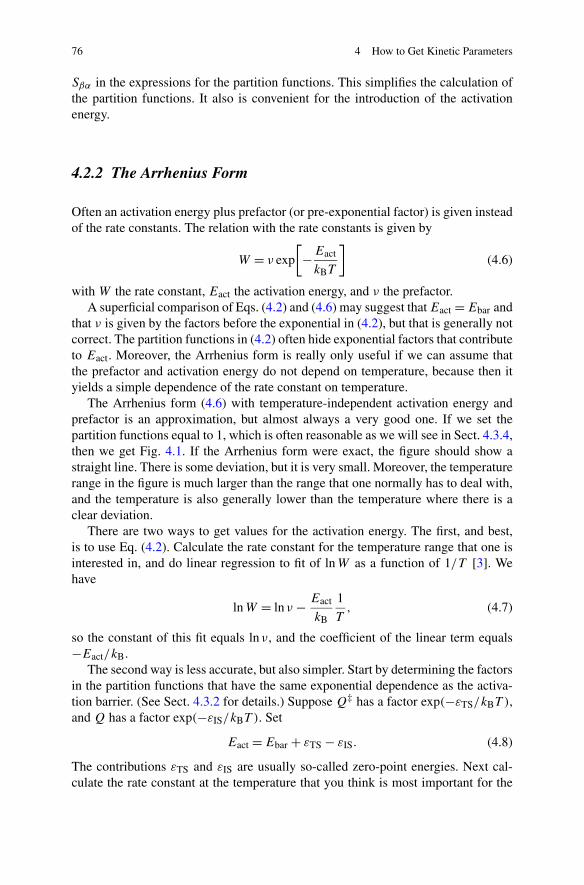
76 4 How to Get Kinetic Parameters

Sβα in the expressions for the partition functions. This simplifies the calculation ofthe partition functions. It also is convenient for the introduction of the activationenergy.

4.2.2 The Arrhenius Form

Often an activation energy plus prefactor (or pre-exponential factor) is given insteadof the rate constants. The relation with the rate constants is given by

W = ν exp

[− Eact

kBT

](4.6)

with W the rate constant, Eact the activation energy, and ν the prefactor.A superficial comparison of Eqs. (4.2) and (4.6) may suggest that Eact = Ebar and

that ν is given by the factors before the exponential in (4.2), but that is generally notcorrect. The partition functions in (4.2) often hide exponential factors that contributeto Eact. Moreover, the Arrhenius form is really only useful if we can assume thatthe prefactor and activation energy do not depend on temperature, because then ityields a simple dependence of the rate constant on temperature.

The Arrhenius form (4.6) with temperature-independent activation energy andprefactor is an approximation, but almost always a very good one. If we set thepartition functions equal to 1, which is often reasonable as we will see in Sect. 4.3.4,then we get Fig. 4.1. If the Arrhenius form were exact, the figure should show astraight line. There is some deviation, but it is very small. Moreover, the temperaturerange in the figure is much larger than the range that one normally has to deal with,and the temperature is also generally lower than the temperature where there is aclear deviation.

There are two ways to get values for the activation energy. The first, and best,is to use Eq. (4.2). Calculate the rate constant for the temperature range that one isinterested in, and do linear regression to fit of lnW as a function of 1/T [3]. Wehave

lnW = lnν − Eact

kB

1

T, (4.7)

so the constant of this fit equals lnν, and the coefficient of the linear term equals−Eact/kB.

The second way is less accurate, but also simpler. Start by determining the factorsin the partition functions that have the same exponential dependence as the activa-tion barrier. (See Sect. 4.3.2 for details.) Suppose Q‡ has a factor exp(−εTS/kBT ),and Q has a factor exp(−εIS/kBT ). Set

Eact = Ebar + εTS − εIS. (4.8)

The contributions εTS and εIS are usually so-called zero-point energies. Next cal-culate the rate constant at the temperature that you think is most important for the

4.2 Two Expressions for Rate Constants 77

Fig. 4.1 The logarithm of the rate constant ln(Wh/Ebar) according to Eq. (4.2) with Q‡ = Q = 1plotted versus reciprocal temperature Ebar/kBT . Although the expression is not linear, the devi-ation of linearity is only very small, and only visible at high temperatures (i.e., small values ofEbar/kBT ). A very similar plot is obtained even if the partition functions can not be approximatedby Q‡ = Q = 1

processes that you are interested in. If we call the calculated rate constant Wcalc,then take ν = Wcalc exp(Eact/kBT ) as prefactor.

Sometimes the activation energy is defined by

Eact = − ∂ lnW

∂(1/kBT )(4.9)

with W given by Eq. (4.2) or a similar expression. This gives Eq. (4.8) for theactivation energy plus some additional term. One should realize that this expressionand the procedures described above are all just definitions of the activation energy.Expression (4.8) has a simple physical interpretation as will be shown in Sect. 4.3,but it leads to an Arrhenius form that is valid over only a limited temperature range.The activation energy derived from the linear regression is valid over a much widertemperature range, but it has no good physical interpretation. Expression (4.9) seemsto be the least useful. It has no good physical interpretation, and it does not yielda simple temperature dependence compared to the Arrhenius form. One may arguethat it is more accurate, but if that is important then one can just is well use the TSTexpression (4.2). Note also that working with activation energy and prefactor is onlyuseful when one wants to do simulations at different temperatures. Otherwise, it iseasier to specify the rate constant directly.

78 4 How to Get Kinetic Parameters

4.3 Partition Functions

Whether one wants just to calculate a rate constant, or compute also activation en-ergies and prefactors explicitly, one needs to compute partition functions. As theyform such an important part of the expression of the rate constants, we will discussthem in some detail.

4.3.1 Classical and Quantum Partition Functions

The derivation of the master equation in Sect. 2.2.2 is based on phase space andthe classical Liouville equation. The expressions for the rate constants (Eqs. (2.32)–(2.34) and (4.2)–(4.4)) are also classical expressions. For some situations this is per-fectly acceptable, but when there are coordinates that correspond to motions with aquantum mechanical excitation energy that is at least of the order of the thermal en-ergy kBT , it is not. Of course, one might try to rederive the master equation startingfrom quantum mechanics, but that is very difficult and seldom necessary. In manycases it suffices to replace expressions (4.3) and (4.4) by their quantum mechani-cal analogue. Indeed, in the following we will discuss first the quantum mechanicalform of a partition function and only then the classical one. One aspect that can beimportant and that is still absent even if one uses quantum mechanical partition func-tions is the effect of tunneling. To deal with this one can use a tunneling correctionfor the rate constants [4–6].

4.3.2 Zero-Point Energy

The main reason for the difference between the activation barrier Ebar and the acti-vation energy Eact is that the partition functions in Eq. (4.2) may contribute to theexponential factor. This is especially true if there are motions that, when treatedquantum mechanically, have an excitation energy that is of the same order of mag-nitude or larger then kBT . Such motions should not be treated classically, and thepartition functions (4.3) and (4.4) should be replaced by quantum mechanical ones.A quantum mechanical partition function can be written as

Q =∞∑

n=0

exp

[− En

kBT

](4.10)

with the summation over all eigenstates of the Hamiltonian of the system (i.e., thesolutions of the time-independent Schrödinger equation) and En the energy of staten [7]. If the we define state n = 0 as the ground state, then we can rewrite this alsoas

Q = exp

[− E0

kBT

] ∞∑

n=0

exp

[−En − E0

kBT

]. (4.11)

4.3 Partition Functions 79

We can combine the first factor on the right-hand-side with the exponential termexp(−Ebar/kBT ) in Eq. (4.2). The summation in Eq. (4.11) will not have such anexponential dependence. The first term in the summation is always equal to 1. Ifthe excitation energies En −E0 for n ≥ 1 are large compared to kBT , then the otherterms are very small and it may be appropriate to neglect them. The summation thenis simply equal to 1. This often happens for vibrations (see Sect. 4.3.4).

The definitions of the partition functions (Eqs. (4.3) and (4.4)) show that theenergies of the states should be taken with respect to a minimum of the potentialenergy. The difference between E0 and this minimum is called the zero-point energy[8]. Equation (4.2) is often written as

W = kBT

h

Q‡

Qexp

[−Ebar + Ezp

kBT

]. (4.12)

Ezp contains all the zero-point energy contributions from the partition functions. Wehave

Ezp = εTS − εIS (4.13)

with εTS the zero-point energy extracted from Q‡ and εIS that from Q (see alsoEq. (4.8)). The quantity Ebar + Ezp is called the zero-point energy corrected acti-vation barrier. The partition function Q‡ and Q are defined by the summation inEq. (4.11): i.e., the reference level of the energy is chosen so that the ground statehas by definition an energy equal to zero. It is very important for the calculation ofthe partition function to be aware if one is using Eq. (4.2) or Eq. (4.12).1

4.3.3 Types of Partition Function

General expressions for partition functions are not very useful. They have to be sim-plified, and for this we need to make some approximations. It depends on the type ofmotion which approximation is appropriate. The type of motion also determines ifwe need to work with the quantum mechanical expression given by Eq. (4.11), or ifwe may use the classical expression Eqs. (4.3) and (4.4). In principle, this dependson the ratio between the excitation energy for a certain motion and the thermal en-ergy kBT . At high temperatures the difference between the quantum mechanical andthe classical expressions becomes negligible.2 This will turn out to be convenient,

1If one determines the activation energy Eact by a linear regression of a set of rate constants atdifferent temperatures, then this energy is not exactly equal to Ebar + Ezp. This is because thefactors (kBT/h)(Q‡/Q) also give a small contribution to Eact. See the discussion at the end ofSect. 4.2.2.2Strictly speaking this is not always true. There may be a factor in the quantum version that isabsent in the classical one, and that is related to the statistics of identical particles. See for examplethe geometry factor in Eqs. (4.22) and (4.23).

80 4 How to Get Kinetic Parameters

because for some motions the quantum mechanical expression is much harder toevaluate than the classical one.

We will split the degrees of freedom of a system in several groups. These groupsallow us to write a partition function as a product.

Q = QtransQrotQvib (4.14)

with Qtrans the partition function of the translations, Qrot the partition function ofthe rotations, and Qvib the partition function of the vibrations.3 These partition func-tions can often be split further. For example, for the vibrations one can often use theharmonic approximation (see Eq. (4.16)). The vibrations can then be decoupled intoso-called normal modes, [9], and we can write

Qvib =∏

n

Q(n)vib (4.15)

where the product is over all normal modes with Q(n)vib the partition function of nor-

mal mode n (see Eq. (4.18) Sect. 4.3.4). Also Qtrans and Qrot can often by decoupledat least partially.

4.3.4 Vibrations

Most degrees of freedom of the molecules involved in a reaction are vibrations. Thepotential energy of such a degree of freedom can be approximated by

V (x) = 1

2mω2x2 (4.16)

with x the coordinate of the degree of freedom, m the corresponding mass, andω some constant, which turns out to be equal to the (angular) frequency of thevibration. The minimum energy of the potential here has been set equal to 0 and x

is defined in such a way that x = 0 corresponds to the position of the minimum ofthe potential. The energies of the states are then given by [8]

En =(

n + 1

2

)�ω (4.17)

with n a non-negative integer.

3There are actually two more factors [7]. There is the partition function of the electronic statesQel and the partition function of the spins of the nuclei Qnucl. We will ignore both. The electronicground state defines the potential energy of the system, so the partition function is defined only bythe summation in Eq. (4.11). As the electronic excitation energies are, except for rare case, muchlarger than the thermal energy, we get Qel = 1. The spin state of the nuclei generally does notchange during a reaction. So its partition functions for the transition and initial state cancel in theexpression for the rate constant, and can therefore be ignored.

4.3 Partition Functions 81

Fig. 4.2 Qvib of Eq. (4.19) as a function of �ω/kBT

The minimum of the potential energy is 0, so the zero-point energy is �ω/2. Thesummation of Eq. (4.11) can be done analytically and the result for the partitionfunction is

Qvib = Qvibe−�ω/2kBT (4.18)

with

Qvib = 1

1 − e−�ω/kBT. (4.19)

The reason to split off Qvib is that exp[−�ω/2kBT ] is a zero-point energy factorthat can be combined with exp(−Ebar/kBT ). Moreover, Qvib can be approximatedby 1 if �ω � kBT , which is quite common. If on the other hand �ω � kBT we haveQvib = kBT/�ω (see Fig. 4.2).

4.3.5 Rotations

There are three different partition functions for rotation that are relevant. If we havea chemical group that rotates around some axis (e.g., CH3), then we have a one-dimensional rotation. If we have a linear molecule in the gas phase (relevant foradsorption and desorption), then we have two rotational degrees of freedom. If wehave a non-linear molecule in the gas phase, then we have even three rotationaldegrees of freedom. There are no closed-form expressions for the quantum me-chanical partition functions, but the rotational excitations are small compared to thethermal energy for almost all molecules and temperatures. So we will give the high-temperature limit of the quantum mechanical expressions [7]. These are equal to theclassical expressions apart from geometric factors.

82 4 How to Get Kinetic Parameters

For a chemical group rotating around an axis we have

Qrot,1D = 2π

h

√2πIkBT (4.20)

with I a moment of inertia that is defined as

I =∑

n

mnr2n. (4.21)

The summation in this expression is over all atoms of the group, and rn is the dis-tance of atom n to the rotation axis and mn the mass of the atom n.

For a freely rotating linear molecule we have4

Qrot,2D = 8π2IkBT

σh2. (4.22)

Here I is again a moment of inertia. It is defined formally again by expression(4.21), but rn is now the distance of atom n to the center of mass of the molecule.The symmetry number σ is 2 for molecules with an inversion center and 1 otherwise.

For a freely rotating non-linear molecule we have

Qrot,3D =√

π

σ

∏

n

√8π2InkBT

h2. (4.23)

The summation is over the principle moments of inertia. These are the eigenvaluesof the matrix with the moments of inertia. This matrix has diagonal components

Iαα =∑

n

mn

[|rn|2 − r2nα

](4.24)

and non-diagonal components

Iαβ =∑

n

mnrnαrnβ. (4.25)

The summation is over all atoms in the molecule, rn is the vector from the center ofmass of the molecule to atom n, and α,β = x, y, z. The symmetry number σ is thenumber of proper rotations in the point group of the molecule.

One can define so-called rotational temperatures θrot for a molecule via

θrot = h2

8π2IkB(4.26)

with I a principle moment of inertia. With this definition we can write

Qrot,2D = 1

σ

T

θrot(4.27)

4Note that below room temperature this expression should not be used for molecular hydrogen.The rotational excitations for this molecule are so high, that the high-temperature approximationonly becomes valid at higher temperatures.

4.3 Partition Functions 83

Table 4.1 Rotational temperatures and geometry factors for some small molecules. There is onlyone temperature for linear molecules. (Note that these temperature are not necessarily very ac-curate. They were calculated assuming a rigid structure of the molecule based on DFT/B3LYPcalculations with a 6-31G+(d) basis set [10])

Molecule θrot,A/K θrot,B/K θrot,C/K θrot,Aθrot,Bθrot,C/K3 σ

H2 87.9 2

CH4 7.60 7.60 7.60 438.2 12

NH3 14.4 14.4 8.97 1856 3

H2O 39.7 20.4 13.5 1089 2

CO 2.73 1

CO2 0.554 2

N2 2.84 2

NO 2.42 1

NO2 11.3 0.619 0.587 4.112 1

and

Qrot,3D =√

π

σ

(T 3

θrot,Aθrot,Bθrot,C

)1/2

(4.28)

with three different rotational temperatures for a non-linear molecule. Table 4.1shows values for some small molecules. The advantage of these temperatures isthat they simplify the calculations of rotational partition functions.

4.3.6 Hindered Rotations

The rotation of a chemical group around an axis is often not completely free, be-cause of steric repulsion or other interactions. For such hindered rotation it is notpossible to give a closed-form expression of the partition function. On the otherhand, because it is only a one-dimensional problem, it is relatively easy to computethe partition function numerically.

The Schrödinger equation for the rotation is given by

HΨn(ϕ) =[−�

2

2I

d2

dϕ2+ V (ϕ)

]Ψn(ϕ) = EnΨn(ϕ) (4.29)

with H the Hamiltonian, ϕ the rotational angle, I the moment of inertia given byEq. (4.21), and V (ϕ) the potential energy that describes the barriers that prevent thefree rotation. The subscript n is a non-negative integer that labels the various solu-tions. The function V might be determined by doing quantum chemical calculationsof the system for various values of ϕ, and then fitting the results to some functionalform: e.g., a Fourier series [11].

To solve this Schrödinger equation we expand the wave functions in a basisand then use the variation principle [12]. It seems obvious to use the geometric

84 4 How to Get Kinetic Parameters

functions sin and cos as a basis, or complex exponential function. Suppose wetake a basis e−iMϕ/

√2π, e−i(M−1)ϕ/

√2π, . . . , e−iϕ/

√2π,1/

√2π, eiϕ/

√2π, . . . ,

ei(M−1)ϕ/√

2π, eiMϕ/√

2π , write

Ψn(ϕ) =M∑

m=−M

eimϕ

√2π

cmn (4.30)

and use the variation principle. We then get

HC = CE (4.31)

with the matrices given by the following definitions of the matrix elements.

Hmn = 1

2π

∫ 2π

0dϕe−imϕHeinϕ, (4.32)

Cmn = cmn, and Emn = Enδmn. So we get an eigenvalue equation with the energiesin the diagonal matrix E and the coefficients of the wave functions in the columnsof the matrix C.

Once the energies have been determined, the partition function then follows im-mediately from Eq. (4.11). Note that the accuracy depends on the size of the basis:i.e., on the value of M . One should increase M until the value of Q does not changeanymore.

4.3.7 Translations

Free translations are rare for surface processes. They are only found when the corru-gation of the surface is very small, and an adsorbate can move almost unhindered insome direction. This can occur either for the initial state of a process or the transitionstate.

The classical partition function is appropriate and quite easy to compute. UsingEq. (4.3) for a one-dimensional translation gives

Qtrans =∫ L

0dx

∫ ∞

−∞dp

hexp

[− p2

2mkBT

]= L

√2πmkBT

h. (4.33)

Note that L is the length of the interval over which the translation is free. In simu-lations it is generally related to the size of an adsorption site (see Sect. 4.4.2). Theexception is adsorption (see Sect. 4.4.3).

4.3.8 Floppy Molecules

A floppy molecule is a molecule with a potential-energy surface (PES) that has manyminima that are separated by barriers that can easily overcome by thermal excitation

4.4 The Practice of Calculating Rate Constants 85

or tunneling. Partition functions for floppy molecules can be quite hard to compute,and we know of no simple expressions or methods that one can use. If the floppy partof a molecule is not involved in the reaction, then one may assume that the motionsof that part are the same in the initial and transition state so that their contributionto the partition functions in Eq. (4.2) cancel. If one really needs to compute thepartition function of a floppy molecule, then free-energy techniques from MolecularDynamics (MD) are probably the most appropriate [13], as the partition function andthe free energy F are related via [7]

F = −kBT lnQ. (4.34)

There are also so-called rare event techniques in MD to compute rate constantsdirectly for floppy molecules [13].

4.4 The Practice of Calculating Rate Constants

The first thing to do before one starts doing any actual calculations, certainly if theyare electronic structure calculations, is to determine which type of process one wantto calculate the rate constant of. For some processes it may not even be necessary todo any calculations.

The general approach is as follows. First, determine the initial state of a process.This is a stable configuration corresponding to a minimum of the PES. Compute theenergy and the partition function (Eq. (4.3)) for that minimum. Next determine thetransition state for the process. Again compute the energy and the partition function(Eq. (4.4) in this case). The difference of the energies is Ebar, and the rate constantcan be computed using Eq. (4.2). The details on how to actually do these calcu-lations is outside the scope of this monograph. Most of the calculations that haveactually been done have been electronic structure calculations about which variousexcellent textbooks have already been written [14–17]. There have been also a fewcalculations based on PES’s [18–20].

4.4.1 Langmuir–Hinshelwood Reactions

The general approach just described is exactly what one has to do for reactions forwhich reactants and products remain on the surface. The hardest part is in generalthe determination of the transition state. Some methods (e.g., the dimer method[21]) only need the initial state as a starting point. Others (e.g., the nudged-elasticband method [22, 23]) also need the final state. In the latter case one only needs tocalculate extra the partition function of the final state and then one can calculate therate constant of the reverse reaction too. The transition state of the reverse reactionand its partition function is of course the same as that of the forward reaction.

The energies of the initial state EIS and the transition state ETS give the acti-vation barrier Ebar = ETS − EIS. To compute the partition functions one should

86 4 How to Get Kinetic Parameters

do calculations of the vibrational frequencies of the initial and the transition state.Before doing such calculations one should determine which degrees of freedom toinclude in the calculation. Vibrations that do not change in a reaction give partitionfunctions that are the same for the initial and the transition state. They cancel inthe expression of the rate constant, and need not be included. It is not always clearwhich degrees of freedom can be left out however. Including too many never givesincorrect results, but is less efficient. Leaving out important degrees of freedom maygive less accurate results, although this is generally much less serious than an errorin the determination of the activation barrier.

After calculating the vibrational frequencies, one should inspect the correspond-ing vibrations. In particular, one should check if all motions actually correspond tovibrations. If that is the case, then the partition functions of the initial and transitionstates are simply products of vibrational partition functions. To be precise, add thezero-point energies of the vibrations of the transition state to the activation barrierEbar and subtract those of the initial state. The partition functions are products ofQvib’s given by Eq. (4.19). Note that the transition state should have one and onlyone vibration with an imaginary frequency (ω2 < 0). Do not include the zero-pointenergy and the partition function of this vibration in the calculation of the rate con-stant.

Very often (kBT/h)(Q‡/Q) ≈ 1013 s−1. This is because there are two limitingcases that accidentally give results of the same order of magnitude. The vibrationalexcitation energies are either of the same order of magnitude as the thermal energy,or they are much larger. In the former case partition functions become approximatelykBT/�ω and (kBT/h)(Q‡/Q) becomes the product of vibrational frequencies ofthe initial state divided by the product of the vibrational frequencies of the transitionstate. The result is generally in the order of 1013 s−1. In the latter case partitionfunction become approximately equal to 1. Now Q‡/Q ≈ 1 and kBT/h is alsoabout 1013 s−1. If one does not want to calculate partition functions, then 1013 s−1

is a good value to take for the prefactor.Really different prefactors are obtained if there is a degree of freedom that is

not a vibration. This can be a rotation (e.g., of a methyl group or a small moleculeas a whole rotating around an axis perpendicular to the surface). If the barrier forrotation is large (i.e., much larger than the thermal energy kBT ), then such a degreeof freedom can be treated as a vibration. If not the vibrational partition functionshould be replaced by expression (4.20) or be treated as a hindered rotation.

4.4.2 Desorption

The reason why desorption needs to be treated differently from Langmuir–Hinshelwood reactions is that often the transition state is equal to the final state:i.e., it is a molecule in the gas phase. If that is not the case, and the transition stateis a structure with the molecule still adsorbed on the surface, then the calculationof the rate constant for desorption can be done in exactly the same way as for a

4.4 The Practice of Calculating Rate Constants 87

Langmuir–Hinshelwood reactions.5 We therefore deal here only with the situationin which the transition state is a molecule in the gas phase.

The activation barrier Ebar in that case equals the adsorption energy. The par-tition functions and the zero-point energy of the initial state can be calculated inexactly the same way as for Langmuir–Hinshelwood reactions. For the molecule inthe gas phase this also holds for the internal vibrations and possible internal degreesof freedom that correspond to rotations of chemical groups. The difference withLangmuir–Hinshelwood reactions is in the motions of the molecule as a whole.A calculation of the vibrations of the molecule will yield five (for a linear molecule)or six vibrations (for a nonlinear molecule) with a frequency that should be exactlyzero. These correspond to overall translations and overall rotations. The zero-pointmotions of both are zero. The partition function for the overall rotation is eithergiven by Eq. (4.22) for a linear molecule or Eq. (4.23) for a non-linear molecule.The overall rotation can yield prefactors for desorption that are substantially largerthan the customary 1013 s−1.

A little bit of care needs to be taken when calculating the partition function ofthe overall translations. Here the limits on the integration over the coordinates inEq. (4.3) become important. The coordinates in that expression are the two center-of-mass coordinates parallel to the substrate, because we take the surface Sβα todistinguish the adsorbed from the desorbed state of course parallel to the substrate.The integration region is the region of an adsorption site. This is because we wantto have the rate constant for desorption from a particular site. Because we choosethe surface Sβα far from the substrate so that the corrugation of the potential isnegligible, the integration of the coordinates is equal to the area of a site Asite. Thisarea is defined as the total area of the substrate divided by the number of sites fromwhich the adsorbate can desorb. (Note that there may be other sites from which nodesorption is possible. These should not be counted here, because it is really thedividing surface Sβα that should be partitioned into areas corresponding to the sitesfrom which desorption takes place.) The partition function for the center-of-massmotion contributing to Q‡ is then a factor 2πmkBT Asite/h2.

In the discussion of adsorption rate constants (Sect. 4.4.3) we will see an ef-fect of recrossing the surface Sβα . This same effect also influences desorption rateconstants as will be shown there.

4.4.3 Adsorption

Because the initial state of adsorption is a molecule in the gas phase, we need toinclude the gas phase if we want to calculate the rate constant for adsorption. Sup-pose our system consists of a gas of just one molecule in a rectangular box, and we

5It may be that there is a very low barrier for diffusion of the adsorbed molecule. In that case thepartition function of the initial or transition state will have a 2D translational partition function forthe center of mass motion as a factor. See the example of CO desorption in Sect. 4.4.6.

88 4 How to Get Kinetic Parameters

are interested in the adsorption of that gas onto one of the interior sides of the box.Suppose this side has an area A and the volume of the box is V .

We first look at adsorption that is not activated: i.e., the surface Sβα is a plane farfrom the side where the adsorption takes place and on which the potential energy isconstant and equal to its value in the gas phase. The partition function (4.3) of thecenter-of-mass is then a product of two translational partition functions of transla-tions parallel to the side. (We can ignore the other degrees of freedom, because theycancel in the two partition functions in Eq. (4.2).) The partition function (4.4) hasa third factor which is the translational partition function of a translation perpen-dicular to the side. The ratio Q‡/Q of the partition functions is then one over thatthird translational partition function. The activation barrier is zero, so Eq. (4.2) foradsorption somewhere on the side becomes

Wads = AkBT

V√

2πmkBT(4.35)

where we have used Eq. (4.33) for the translational partition function and L = V/A.It looks as if this depends on the actual size of the box, but that is not the case.

First we have PV = kBT with P the pressure exerted by the single molecule. Sec-ond for a kMC simulation we do not want to know the rate constant for adsorptionsomewhere on the side, but at a particular site. We have to divide therefore by thenumber of sites. This then yields

Wads = PAsite√2πmkBT

(4.36)

with Asite the area of a single site. (Asite is really the area A divided by the numberof ways a molecule may adsorb. This number is not always equal to the number ofsites. For example, when we have dissociative adsorption it is two or four times thenumber of sites depending on whether the fragments of the dissociation are the sameor not.) Although we have derived this expression for a gas with just one molecule, italso holds if there are more molecules. The only thing that changes is the numericalvalue of the pressure P . The expression can also be derived by determining thenumber of molecules that hit the side per unit time. The expression is very simple,and none of the quantities need to be determined via an extensive computation.

If the adsorption is activated (i.e., there is a transition state), then the resultschange substantially. We start again with just one molecule in the gas phase. Therate constant for adsorption on a specific site becomes

Wads = kBT

h

Q‡

QtransQrot,3DQintexp

[−Ebar

kBT

]. (4.37)

Here Qtrans is the translational partition function for the center-of-mass of moleculein the gas phase, Qrot,3D its partition function for its overall rotation, and Qint for itsinternal motions (probably lots of vibrations, but maybe also rotations of chemicalgroups, etc.). For Qrot,3D Eq. (4.23) holds, and Qint can be written as a product

4.4 The Practice of Calculating Rate Constants 89

of function of the type (4.19) and possibly (4.20). (Note that the vibrations yieldzero-point energies.) For the Qtrans we have

Qtrans = V

[2πmkBT

h2

]3/2

. (4.38)

If we substitute this in the expression for the rate constant and use PV = kBT again,we get

Wads = h2P

(2πmkBT )3/2

Q‡

Qrot,3DQintexp

[−Ebar

kBT

]. (4.39)

As before this expression also holds for a gas consisting of many molecule. Onlythe numerical value of the pressure P is different.

If we compare a molecule in the gas phase with a molecule adsorbed on the sur-face, we note that the molecule can freely translate and rotate in the gas phase, butnot when adsorbed. This means that the molecule in the gas phase has a higherentropy then when it is adsorbed. This should of course affect the adsorption-desorption equilibrium, and also the rate constants for adsorption and desorption.Remarkably, only one of these rate constants is affected, but which one depends onthe transition state. If there is no transition state (or what is the same thing, the finaland transition state corresponding to the molecule in the gas phase), then the desorp-tion rate constant is large. This is because of the increase of rotational entropy in thetransition/final state upon desorption. The adsorption rate constant on the other handhas a normal value given by the number of molecules in the gas hitting the substrateper unit time. If there is a transition state in which the molecule is adsorbed on thesubstrate, then the desorption rate constant has a normal value, but the adsorptionrate constant is small. This is because the molecule loses rotational entropy when itadsorbs. In both cases the molecule loses translation entropy when it adsorbs.

Note that the expression for the adsorption rate constant does not contain a stick-ing coefficient. This coefficient reflects the influence of trajectories in phase spacethat cross and then recross the dividing surface as explained at the end of Sect. 2.2.2.So far we have neglected this phenomenon, assuming that its effect on the rate con-stant is negligible. For adsorption this is often not the case, and an extra factor σ

should be added to the expressions for the adsorption rate constant. This σ is thesticking coefficient.

Figure 4.3 shows characteristic trajectories and how they give rise to the stickingcoefficient. Trajectory 1 is a regular adsorption. Trajectory 2 shows a molecule beingscattered from the substrate leading to a recrossing of the dividing surface. Thistrajectory should not be included in the calculation of the adsorption rate constant,but Eqs. (4.36) and (4.39) however do not exclude it. These equations include theeffect of crossings at 1+, 2+, and 3+. The effect of the last is probably negligible, butthe effect of 2+ is not. By introducing a sticking coefficient σ we have the effects ofthe crossings at 2− and 3− cancel those of the crossings at 2+ and 3+, respectively.

Note that the crossings at 2−, 3−, 4− all affect the rate constant of desorption,whereas only the one at 4− constitute a real desorption. This means that the expres-sions for desorption should also be corrected for recrossings. It turns out that this

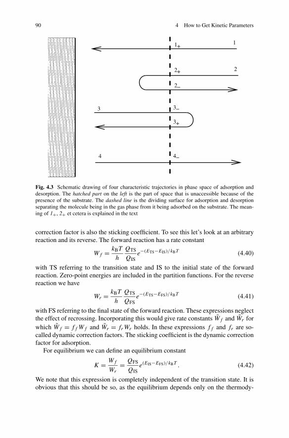
90 4 How to Get Kinetic Parameters

Fig. 4.3 Schematic drawing of four characteristic trajectories in phase space of adsorption anddesorption. The hatched part on the left is the part of space that is unaccessible because of thepresence of the substrate. The dashed line is the dividing surface for adsorption and desorptionseparating the molecule being in the gas phase from it being adsorbed on the substrate. The mean-ing of 1+, 2+ et cetera is explained in the text

correction factor is also the sticking coefficient. To see this let’s look at an arbitraryreaction and its reverse. The forward reaction has a rate constant

Wf = kBT

h

QTS

QISe−(ETS−EIS)/kBT (4.40)

with TS referring to the transition state and IS to the initial state of the forwardreaction. Zero-point energies are included in the partition functions. For the reversereaction we have

Wr = kBT

h

QTS

QFSe−(ETS−EFS)/kBT (4.41)

with FS referring to the final state of the forward reaction. These expressions neglectthe effect of recrossing. Incorporating this would give rate constants Wf and Wr forwhich Wf = ff Wf and Wr = frWr holds. In these expressions ff and fr are so-called dynamic correction factors. The sticking coefficient is the dynamic correctionfactor for adsorption.

For equilibrium we can define an equilibrium constant

K = Wf

Wr

= QFS

QISe(EIS−EFS)/kBT . (4.42)

We note that this expression is completely independent of the transition state. It isobvious that this should be so, as the equilibrium depends only on the thermody-

4.4 The Practice of Calculating Rate Constants 91

namic properties of the initial and final states. This has an important consequence,because also the shape of the trajectories at the dividing surface (i.e., recrossings)do also not affect the equilibrium, and we must also have

K = Wf

Wr

. (4.43)

Consequently, ff = fr must hold as well: i.e., the dynamic correction factors for areaction and its reverse are the same. For an adsorption-desorption equilibrium thismeans that including a sticking coefficient in the adsorption rate constant forces usto include it also in the desorption rate constant, as otherwise we get an incorrectequilibrium.

4.4.4 Eley–Rideal Reactions

Eley–Rideal reactions have expressions for the rate constant that are very similarto those of activated adsorption. The difference is that in expression (4.39) for theEley–Rideal reaction P , m, Qrot,3D, and Qint refer only to the reactant in the gasphase, that there is another partition function in the denominator for the degrees offreedom of the adsorbed reactant, and that Q‡ contains the degrees of freedom ofthe atoms of both reactants.

4.4.5 Diffusion

In the lattice-gas model diffusion is represented as a hopping of an adsorbate fromone site to a neighboring one. The calculation of rate constants for diffusion canthen be done in exactly the same way as for Langmuir–Hinshelwood reactions.

4.4.6 Examples

To illustrate how rate constants are actually calculated we will discuss a few exam-ples. Note that not all numbers have really been computed. In those instances wheredata is missing we will guesstimated the numbers. This does not affect the mannerin which the rate constant are computed in any way.

Let’s start with what is the most common case by looking at the reaction NH2 →NH + H on a Rh(111) surface [24]. Density-Functional Theory (DFT) calculationshave shown that NH2 prefers to adsorb on a bridge site. NH on the other hand prefersan fcc hollow site and the H atom that is formed in this reaction also ends up at an fcchollow site. A nudged-elastic band calculation was used to determine the transitionstate. This gave an activation barrier of Ebar = 1.07 eV. The vibrational frequencies

92 4 How to Get Kinetic Parameters

were calculated for both NH2 at a bridge site, and for the transition state. Only theatoms of the adsorbates were allowed to move. These calculations gave a zero-pointenergy correction of Ezp = −0.23 eV. Inspection of the vibrations showed that allmotions were indeed vibrations, so that the partition functions of Eq. (4.2) could bewritten as products of vibrational partition functions. It was found that Q‡/Q ≈ 1.With these results rate constants were calculated between 100 K and 1000 K. Linearregression of the logarithm of the rate constant as a function of 1/T then gave anactivation energy Eact = 0.86 eV and a prefactor ν = 1.68 ·1013 s−1. There is a smalldifference of 0.02 eV between Eact and the zero-point energy corrected activationbarrier Ebar + Ezp.

In the previous example the partition functions Q and Q‡ are very close to 1. Wehave typically found that the rate constant varies not more than a factor of about 3, aslong as the motions of the adsorbates are all vibrations. For the reaction NH2 +H →NH3 on Rh(111) the effect is much larger however. All calculations for this reactionwere done in the same way as for the previous example. (Both reactions were partof an extensive study on the dehydrogenation and oxidation of NH3 on rhodium[24, 25].) The essential difference in the new reaction is that in the transition stateNH3 has almost its equilibrium geometry. In particular, there is a free rotation ofNH3 around its three-fold axis. This rotation was treated as a 1D rotation with apartition function give by Eq. (4.20). All other motions were vibrations. Becauseof this 1D rotation, the partition function of the transition state Q‡ became muchlarger than when there would be only vibrations. Proceeding as for NH2 → NH+H,except for the replacement of one vibrational partition function by Qrot,1D, it wasfound that Eact = 1.10 eV and ν = 1.90 · 1015 s−1. Note the substantially largerprefactor due to the gain in rotation entropy in the transition state. The differencebetween Eact and Ebar + Ezp was not affected by this rotation: it was only 0.04 eV.

There have been extensive studies of CO on numerous transition metal surfaces.We look at desorption of CO from Rh(100) assuming that the transition state isequal to the final state: i.e., CO in the gas phase. The calculated adsorption en-ergy, and therefore also the activation barrier, is 1.85 eV [26]. In the initial state allthe motions are vibrations. The experimental C-O stretch vibration is 1990 cm−1

and the metal-CO stretch is 470 cm−1 [27]. Let’s assume that the other four vi-brations of CO are 250 cm−1 based on a comparison with NO/Rh(100) [28]. Asa consequence the zero-point energy is 0.43 eV, and Q = 19.5 at T = 500 K,which is the peak maximum temperature of the Temperature-Programmed Des-orption (TPD) spectrum at low coverage [27]. For the transition state we have aproduct of three different partition functions. There is a vibrational one Qvib for theC-O stretch. The second is the rotational Qrot,2D. The third is a 2D translationalone Qtrans. The stretch vibration gives a zero-point energy of 0.27 eV, so that thezero-point energy corrected activation barrier is 1.69 eV. We have Qvib = 1.003 atT = 500 K, Qrot,2D = 191.5 (see Eq. (4.22) with I = 1.542 · 10−46 kg.m2), andQtrans = 2πmkBT Asite/h2 = 341.0 (with Asite = 7.43 · 10−20 m2). Consequently,Q‡ = 6.55 · 104. With ν = (kBT/h)(Q‡/Q) = 3.5 · 1016 s−1. For the adsorption ofCO onto the same surface we can use Eq. (4.36). Again at T = 500 K and a pressureof P = 1 atm we get Wads = 1.68 · 108 s−1.

4.4 The Practice of Calculating Rate Constants 93

It is interesting to compare the result for the desorption rate constant to experi-mental results and look at the consequences for the adsorption rate constant. TPDexperiments give Eact = 1.44 eV and ν = 3.98 ·1013 s−1 [27]. It looks at first glancethat there is a substantial difference between the calculated and the experimentalvalues. However, if we would use the calculated parameters to simulate the TPDspectra we would find peaks that are almost at the same temperature as in the exper-iment, but only somewhat narrower. The experimental activation energy and pref-actor give a rate constant for desorption at T = 500 K of 0.122 s−1. The calculatedrate constant is 0.515 s−1. This differs only by a factor of 4.2. (Remarkable there is amolecular beam experiment that does give a prefactor that is close to the calculatedone [29].) There is clearly a compensating effect in the derivations of the activa-tion energy and the prefactor. The difference between the activation energy and theadsorption energy above may be due to errors in the DFT calculations. A possibleexplanation for the large discrepancy in the prefactor is that our assumptions of atransition state of CO in the gas phase is incorrect. An alternative explanation is thatthe motion of the center of mass of the adsorbed CO parallel to the surface con-sists not of two vibrations, but of a free 2D translation. Instead of two vibrationalpartition functions we then get a 2D translational partition function. This causes anincrease of Q by a factor of 340, and makes the prefactor 1.03 · 1014 s−1. Note thatthen also part of the zero-point correction disappears, which unfortunately increasesthe discrepancy between calculated and experimental activation energy.

The calculated prefactor for the desorption is a factor 880 too large. Yet anotherexplanation is related to the adsorption. The reason is that the adsorption-desorptionequilibrium does not depend on the transition state, and hence neither does the ratiobetween the rate constants for adsorption and desorption. This means that if the des-orption prefactor is too large then so is the adsorption rate constant. The reason whythe latter may be too large is that the sticking coefficient may be small. So the cal-culated prefactor for desorption may be too large, because trajectories of scatteredCO molecules may be been included in that calculation. See Sect. 4.4.3 for a moreextensive discussion of this.

4.4.7 Summary

The previous sections describe the most common way to calculate the rate constantsof different types of processes. There are however exceptional cases as the discus-sion of the CO desorption from Rh(100) in Sect. 4.4.6 shows. We will attempt hereto describe a systematic approach.

Do the following for the initial and transition state. First, look at the overalltranslations: i.e., the motions of the center of mass of a molecule. Are some of thesedegrees of freedom free: i.e., is the PES (nearly) flat for those degrees of freedom? Ifyes, use a translational partition function for those degrees of freedom. If not, thesedegrees of freedom become part of the group of vibrational degrees of freedom.

Second, look at the overall rotations: i.e., rotations in which the structure of themolecule remains the same. Are some of these degrees of freedom free or possible

94 4 How to Get Kinetic Parameters

but hindered? If yes, use a rotational partition function for those degrees of freedom.If not, these degrees of freedom too become part of the group of vibrational degreesof freedom. The particular rotational partition function that one needs to use dependson whether the molecule is linear or nonlinear, on the number of axes around whichthe molecule can rotate freely, and on whether the rotation is hindered or not.

Third, take the vibrational degrees of freedom obtained from inspecting the over-all translations and rotations and add the internal degrees of freedom. All thesedegrees of freedom may be coupled. Do a vibrational analysis of them. If the vi-brational analysis gives only normal modes that are indeed vibrations, then use vi-brational partition functions for them. If some of them are rotations of chemicalgroups, use 1D rotational partition functions or the partition functions of a hinderedrotation. If some of them correspond to a floppy motion, then consider using theMD techniques mentioned in Sect. 4.3.8.

Fourth, for vibrational degrees of freedom one should use the partition functiondefined by the summation in Eq. (4.11). Add the zero-point energy of the vibrationof the transition state to the activation barrier, and subtract those of the initial state.

Fifth, combine all partition functions and energies according to Eq. (4.12) tocompute the rate constant.

4.5 Lateral Interactions

Interactions between adsorbates, or lateral interactions have at least been known foras long as diffraction techniques have revealed that adlayers can form very well-defined structures at low temperatures. The importance of these interactions for ki-netics at higher temperatures has only more recently been acknowledged, but formsnow an active area of research. This is understandable if one realizes that even smallinteractions between adsorbates can be of the same magnitude or larger than thethermal energy, and can therefore change rate constants by an order of magnitudeor more, especially at low temperatures.

It is now possible to do quantum chemical calculations on quite realistic mod-els of adsorbates on transition metal surfaces especially using DFT. However, manylateral interactions are small, and although it may be possible to get a value for aparticular lateral interaction using DFT, it does not mean that the result is accu-rate. One should therefore always determine if a particular lateral interaction can becalculated reliably at all.

4.5.1 The Cluster Expansion

Lateral interactions are most commonly described with a cluster expansion. Theadsorption energy Eads per adsorbate in a particular adlayer structure is then writtenas

4.5 Lateral Interactions 95

Eads =∑

m

cmVm (4.44)

with Vm the value of the interaction of type m, and cm the number of interactionsof type m per adsorbate. The interactions Vm stand for the interaction of the ad-sorbate with the substrate (adsorption energy of an isolated adsorbate), pair inter-actions between adsorbates at various distances, all possible three-particle interac-tions, four-particle interactions, et cetera. This expansion can be made to reproducethe calculated adsorption energy as accurately as one wants [30]. This generallytakes however a very large number of terms. Moreover, it may lead to overfitting:i.e., the cluster expansion will not only describe the interactions, but also the errorsone makes in the calculation of the adsorption energies. This occurs because errorsin the calculated Eads can easily be as large or even larger than some Vm’s. To avoidthis one needs to truncate the cluster expansion. We will call a particular choice ofVm’s that one includes in the summation of Eq. (4.44) an interaction model.

The truncation of the cluster expansion for lateral interactions between adsor-bates has so far mainly been done based on the desired accuracy with which thetruncated expansion should reproduce the calculated results, the number of accept-able terms in the expansion, the type of terms in the expansion (pair, three-particle,et cetera), the estimated accuracy of the calculated results, and possibly other fac-tors. Often these factors involve a trade-off: e.g., one prefers a short expansion, butit should also have a certain accuracy. Researchers have usually dealt with this usingtheir personal experience and insight, and few objective criteria have been used. Wewill here describe two statistical techniques that do yield such criteria for truncatingthe cluster expansion.

There are a few useful remarks we can make independently of the method thatwe use to determine the lateral interactions. Let’s define

Efitads(n) =

∑

m

cm(n)Vm (4.45)

with n indicating the various adlayer structures that we use to determine the lateralinteractions, and cm(n) the number of interactions of type m per adsorbate in struc-ture n. If Ecalc

ads (n) is the calculated adsorption energy per adsorbate in structure n,then we want the difference between the Efit

ads(n)’s and Ecalcads (n)’s to be as small as

possible. Let’s also define the errors

εn = Efitads(n) − Ecalc

ads (n). (4.46)

These errors need not be independent. There may be a systematic component σ thatis the same for all adlayer structures, and a rest ρn = εn − σ that is independent.The systematic error may be caused by a specific shortcoming of the calculationsof the adsorption energy (e.g., incorrect description of van-der-Waals interactions inDFT), but that need not be the case. Here it is just a numerical error common to allcalculations.

96 4 How to Get Kinetic Parameters

If there is only one adsorbate adsorbing at one type of site, then we can write foreach adlayer structure

Ecalcads (n) = (V0 − σ) +

(∑

m>0

cm(n)Vm − ρn

)(4.47)

with V0 the adsorption energy of an isolated adsorbate, because c0(n) = 1 for allstructures n. We see that the terms that differ for various adlayer structures are notaffected by the systematic error σ . These terms are also the only ones that containthe lateral interactions. This means that the systematic error does not affect the lat-eral interactions. They depend only on the smaller random errors ρn. Consequentlylateral interactions can be determined better than one might suppose having someidea of the accuracy with which one can compute adsorption energies. The system-atic error affects only V0.

The expression above does not hold when there are different adsorbates or whenthere is adsorption on different types of site. The conclusion drawn above still holdshowever. This can be seen as follows. Suppose V0,V1, . . . , VA are the adsorptionenergies originating from various isolated adsorbates and adsorption sites. BecauseEads is the adsorption energy per adsorbate, we have c0(n)+c1(n)+ . . .+cA(n) = 1for all structures n. We can therefore write

Ecalcads (n) =

(A∑

m=0

cm(n)(Vm − σ)

)+(∑

m>A

cm(n)Vm − ρn

). (4.48)

This shows again that a change in the calculated adsorption energies Ecalcads (n) that

can be represented by a change in the systematic error σ gives the same errors εn

with a corresponding change in the adsorption energies V0,V1, . . . , VA, but with thesame lateral interactions.

Looking at errors as above also shows that singling out one adlayer structure, sayn = 1, to determine the adsorption energy of an isolated adsorbate V0 is not a goodidea. Because then we would have E

(1)fit = E

(1)calc = V0 and work with E

(n)calc − E

(1)calc

to determine the lateral interactions. However

Ecalcads (n) − E

(1)calc = (Efit

ads(n) − Efitads(1)

)− (ρn − ρ1). (4.49)

We see that Ecalcads (n) − E

(1)calc has a different error from Ecalc

ads (n). In fact, as the ρ’sare independent ρn − ρ1 has a standard deviation that is

√2 times the one of ρn.

Consequently the errors we will make in the determination of the lateral interactionswill also be a factor

√2 larger. It is better to treat the adsorption energy V0 in the

same way as the lateral interaction parameters.

4.5.2 Linear Regression

Suppose one has determined which Vm’s in Eq. (4.44) should be included, then thereremains the problem of computing their values. Because the adsorption energy Eads

4.5 Lateral Interactions 97

depends linearly on the Vm’s, they can be determined using linear regression [3].This means we use a least-squares approach by minimizing

χ2 = 1

Nstr

∑

n

[∑

m

cm(n)Vm − Ecalcads (n)

]2

(4.50)

as a function of the Vm’s.Differentiating the expression with respect to the different Vm’s and equating the

results to zero gives the so-called normal equations∑

m

αkmVm = βk (4.51)

with

αkm =∑

n

ck(n)cm(n) (4.52)

and

βk =∑

n

ck(n)Ecalcads (n) (4.53)

from which we can determine the Vm’s. We refer to the literature for discussions onproblems with these equations because they may be (approximately) linear depen-dent, and how to deal with this [3]. It should however be obvious that if one hasNstr different adlayer structures, that one certainly will not be able to compute morethan Nstr different Vm’s. In general Nstr should be much larger than the numberof Vm’s.

If the matrix α of the normal equations is not (approximately) singular, then itcan be used to get an idea of how well the Vm’s are determined. The inverse matrixof α has matrix elements that are proportional to the covariances of the Vm’s. Inparticular, the diagonal elements of α−1 are proportional to the standard errors forthe Vm’s. The proportionality constant is equal to χ2.

4.5.3 Cross Validation

The truncation problem of the cluster expansion has been earlier encountered forthe calculation of interactions between atoms forming an alloy. This has led to thedevelopment of the leave-one-out cross-validation (LOO-CV) method [31, 32]. Thisis a statistical technique that uses part of the results of a set of calculations to deter-mine values for the interactions between the atoms and the rest of the calculationsto test these values. Because determination and testing of the interactions is done onindependent results of calculations, one obtains an estimate of how well the valuesfor the interactions one calculates will predict energies of unknown structures. Thismethod has recently also been applied to the determination of lateral interactions[33–35].

98 4 How to Get Kinetic Parameters

The LOO-CV method works as follows [31, 32, 36]. We take all structures exceptone structure n. We then do a linear regression for a particular interaction model (i.e.,a set of Vm’s) using these structures. This gives us a set of interaction parametersthat we can use to predict the adsorption energy for structure n. We then comparethis energy E

predads (n) with the calculated energy Ecalc

ads (n). We do this not just for onestructure n but for all structures, and define the cross-validation score or leave-one-out error

R2CV = 1

Nstr

Nstr∑

n=1

[E

predads (n) − Ecalc

ads (n)]2

. (4.54)

This error indicates how well an interaction model predicts the energy. One startswith a model with few interaction parameters, and determines the CV score. Addingparameters will initially lower the CV score, which means that the model becomesbetter. Adding too many parameter should however increase the CV score becauseof overfitting.

If the number of structures n is large, one may not want to leave out every struc-ture n, determine the lateral interactions, and compare E

predads (n) to Ecalc

ads (n). Insteadone can partition all structures into groups. Each structure should be in one andonly one group. One does the same as for LOO, but now one leaves out all struc-tures in one group instead of just one structure. This is called the leave-many-out(LMO) method. The groups are generally made of similar size, but the structuresare partitioned randomly [36].

The minimum of the CV score indicates a best set of interaction parameters. Theproblem with the method is that often the CV score becomes almost constant whenmore parameters are added, and it is very hard to determine the minimum of the CVscore [37–40].

4.5.4 Bayesian Model Selection

An alternative solution to the truncation problem can be obtained using Bayesianstatistics [37, 41].6 Instead of the CV score of the LOO-CV method, one assignsa probability to each interaction model. The best model is the one with the high-est probability. This approach does not have the drawback of the LOO-CV method.Moreover, it seems that the approach leads to models with fewer interaction param-eters. The method also lends itself well to an analysis of the importance of param-eters: it is easy to compute probabilities for individual parameters, and correlationbetween parameters.

6Parts of Sect. 4.5.4 have been reprinted with permission from A.P.J. Jansen, C. Popa, Bayesianapproach to the calculation of lateral interactions: NO/Rh(111), Phys. Rev. B 78, 085404 (2008).Copyright 2008, American Physical Society.

4.5 Lateral Interactions 99

We assume again that we have done calculations resulting in the adsorption en-ergy per adsorbate Ecalc

ads (n) with n an index to distinguish the adlayer structures,and we describe the energy Ecalc

ads (n) using a cluster expansion for the lateral inter-actions. The expression (4.45) for Efit

ads(n) should approximate Ecalcads (n) as well as

possible. Let’s use S to indicate a subset of all interaction parameters Vm: i.e., itindicates the interaction model. Let’s use V as a shorthand for the set of all val-ues of the interaction parameters in S. For all calculated adsorption energies weuse E. We will determine which interaction model is best by calculating P(S|E),which stands for the probability that the calculated adsorption energies E can bedescribed by interaction parameters in S. The best interaction model has the highestP(S|E).

We can use Bayes’s theorem to relate the probability of S given E (i.e., P(S|E))to the probability of E given S (i.e., P(E|S)) [42–44].

P(S|E) ∝ P(E|S)P (S). (4.55)

The proportionality constant that is missing in this expression can be determinedby normalizing P(S|E) as a function of S. The probability P(E|S) is often calledthe likelihood of S given E, the probability P(S) is called the prior (probability)of S, and the probability P(S|E) is called the posterior (probability). The likeli-hood P(E|S) is the probability that we should find certain values Ecalc

ads (n) if theinteraction model S is the right one. We will determine this from P(E|S,V ): i.e.,we not only know which parameters are in the interaction model, but also their val-ues (see also Eq. (4.58)). The prior P(S) represents what we think are plausiblemodels before we look at the results of our calculations.

Bayes’s theorem is used as follows in the selection of models for the lateral inter-actions. We want to calculate P(S|E). How good an interaction model is will alsodepend on whether we can find good values for the lateral interactions. It is impor-tant to distinguish between S (the parameters in the model) and V (the values ofthese parameters). We can introduce the values by regarding P(E|S) as a marginaldistribution of P(E,V |S) via [44]

P(E|S) =∫

dV P (E,V |S) (4.56)

where the integration is over all possible values for the interaction parameters. Theintegrand can be written as

P(E,V |S) = P(E|S,V )P (V |S). (4.57)

Substitution in the Bayes’s expression for P(S|E) then gives

P(S|E) ∝ P(S)

∫dV P (E|S,V )P (V |S). (4.58)

This allows us to compute P(S|E), because we can make a good guess of whatthe calculated adsorption energies should be given the lateral interactions (i.e.,P(E|S,V )), and it should be possible to think of reasonable priors P(V |S) andP(S).

100 4 How to Get Kinetic Parameters

Suppose we have a set of interaction parameters S with values V . A normalway to obtain such a set is via a least-squares procedure to fit Efit

ads(n) to Ecalcads (n).

Suppose that the set has all interaction parameters to describe the system and thatthey have the correct values. The most likely values for Ecalc

ads (n) should then beequal to Efit

ads(n). Due to errors in the calculations Efitads(n) and Ecalc

ads (n) will not beexactly equal. It can be shown using the Maximum Entropy Principle (MEP) thatif we have no information on the difference, it can best be described by a Gaussianprobability distribution [42]: i.e.,

P(E|S,V ) = exp

[−1

2χ2

1

] Nstr∏

n=1

1√2πσ 2

n

(4.59)

with

χ21 =

Nstr∑

n=1

[Efit

ads(n) − Ecalcads (n)

σn

]2

, (4.60)

Nstr the number of adlayer structures for which we have calculated adsorption ener-gies, and σn an error estimate of the calculated adsorption energies Ecalc

ads (n). Notethat P(E|S,V ) is a function of the adsorption energies Ecalc

ads (n), but the integrationin Eq. (4.58) is over V . This means that we should regard χ2

1 as a function of theinteraction parameters V .

Usually one does not know much about the interaction parameters before onestarts with the calculations of the adsorption energies, nor about which interactionparameters to include in the model. Ideas on which model S is appropriate are splitin Eq. (4.58) from ideas on which values V seem reasonable. The former have a priorP(S), the latter a prior P(V |S). The MEP shows again that the best expression forP(V |S), which is also computationally convenient, is a Gaussian distribution [42]

P(V |S) = exp

[−1

2χ2

2

] Npar∏

m=1

1√2πs2

m

(4.61)

with

χ22 =

Npar∑

m=1

[− (Vm − V

(0)m )2

s2m

], (4.62)

Npar the number of parameters in the interaction model, V(0)m the most likely prior

value for parameter m, and sm the standard deviation. The lack of prior knowledgeof the values of the interactions can be implemented by choosing large values forthese deviations. We find it harder to give a general expression for P(S). If a modelcontains a pair interaction for adsorbates at a certain distance, then pair interactionsat shorter distances should be included as well. Also, if there is a three-particleinteraction in a model, then all pair interactions between these three particles havingsuch three-particle interaction should be included too. One also will want to cut offthe summation in Eq. (4.45). Apart from these considerations it seems natural totake all interaction models equally likely.

4.5 Lateral Interactions 101

The integration in Eq. (4.58) can be done easily because the integrand is a Gaus-sian expression in the integration variables. We define a column vector c via cn =Ecalc

ads (n), a column vector e via en = Efitads(n), and a matrix A via Anm = σ−2

n δnm.With these we can write χ2

1 = (e − c)T A(e − c). The fitted adsorption energies ecan be written as e = Mv with v a column vector with the interaction parameters(vm = Vm), and the matrix M contains the coefficients of the interaction parame-ters in Eq. (4.45). Similarly we write χ2

2 = (v − v)T B(v − v), with vn = V(0)n and

Bnm = s−2m δnm. We can combine χ2

1 and χ22 , and write the result as a quadratic

function of the interaction parameters. This gives us

χ21 + χ2

2 = (v − v)T[MT AM + B

](v − v) + μ, (4.63)

with

v = [MT AM + B]−1(MT Ac + Bv

), (4.64)

and

μ = cT Ac + vT Bv − vT[MT AM + B

]v. (4.65)

With this expression the integration in Eq. (4.58) then becomes

P(S|E) = P(S)

P (E)

1√∏n(2πσ 2

n )

Npar∏

m=1

[sm

sm

]e−μ/2, (4.66)

with 1/s2m being an eigenvalue of the matrix MT AM + B.

Equation (4.66) can be interpreted as follows. The probability of an interactionmodel is higher when μ is smaller. If we assume that the prior distribution P(V |S)

is very broad, so that we can set B = 0, then χ22 = 0, v minimizes χ2

1 , and μ isthe least-squares sum of the difference between the calculated and fitted adsorptionenergies. This means that the probability P(S|E) become higher if the fit becomesbetter. This is of course as it should be.

The probability P(S|E) also becomes higher when the prior errors sm becomesmaller. This too is to be expected, because it more-or-less means that we know aparameter already in advance. Less easy to interpret is the dependence on the s2

m’s.It seems that a high value for sm would improve the model. This however would beincorrect, and is also counter-intuitive. As will be shown below the sm’s are errorestimates for a set of statistically independent interaction parameters. So a highvalue for sm would mean a parameter that is ill-defined, which one would not expectto improve an interaction model. The solution of this paradox is hidden in μ whichalso depends on the sm’s. To see this let’s compare two interaction models S(1) andS(2) with the difference that S(2) has one additional parameter compared to S(1).Let’s also assume, for simplicity, they have the same prior (P(S(2)) = P(S(1))), thatB = 0, and that this additional parameter is independent from the others. This meansthat each sm of S(1) is also found for S(2), but S(2) has an additional factor in theproduct of Eq. (4.66) which we call sN . We then get

P(S(2)|E)

P (S(1)|E)= sN

sNe−(μ(2)−μ(1))/2 (4.67)

102 4 How to Get Kinetic Parameters

with μ(n) the least-squares sum for S(n). When the additional parameter in S(2)

is independent from the others, the matrix MT AM blocks and μ(2) − μ(1) =−(MT AM)NN(vN)2 holds. This leads to

P(S(2)|E)

P (S(1)|E)= sN

sNe(vN/sN )2/2. (4.68)

This function is for small values of sN a decreasing function. Consequently, ifthe interaction parameters are defined better (i.e., smaller sm), then the probabil-ity P(S|E) becomes higher, again as expected. Equation (4.68) shows also howadding a parameter can reduce the probability of an interaction model, because theratio sN/sN will usually be smaller than one, because the error estimates in the priorP(V |S) will be large.

The results above depend on the error estimates σn. This means that the pos-terior really has these estimates as a parameter and should be written P(S|E,σ).Because we need to know the σn’s but have no good information on them, theyare often called nuisance parameters. There are various ways to deal with this[43, 44]. We find it the most convenient to put σn = σ for all n and to get a valuefor σ by determining the maximum of its probability distribution P(σ |E). Thisprobability can be related to probability distributions that we have dealt with be-fore.

P(σ |E) ∝ P(σ)∑

S

∫dV P (E|S,V,σ )P (S,V |σ). (4.69)

P(E|S,V,σ ) is given by Eq. (4.59) and P(S,V |σ) by Eq. (4.61). The proportion-ality constant can be determined by normalization. Only P(σ) is new. However, ifwe assume that it is a uniform distribution then we only need to do the integral andsum over all models. The integral has already been done before, so we only need toadd all results for the different models.

The parameters V(0)m and sm can also be regarded as nuisance parameters, but

it is more convenient to handle them differently. We do not want to use any priorinformation for the interaction parameters, so we take large values for the errorestimates sm. As a consequence the values that we take for the V

(0)m ’s have then only

a negligible effect on the final results,Once we have determined S we also need the parameters V . For this we can

used P(S,V |E), which equals P(E|S,V )P (S,V ). We have already seen the twofactors in this product: the only difference with what we have done before is that wedo not need to integrate out the interaction parameters. The interaction parametersthemselves can be obtained from P(S,V |E) by computing the expectation valuesof V . The derivation above shows that the parameters should be chosen equal tocomponents of the vector v. P(S,V |E) can give us also error estimates for theparameters: the covariance matrix is given by (MT AM + B)−1.

4.5 Lateral Interactions 103

4.5.5 The Effect of Lateral Interactions on Transition States

The previous sections have dealt with equilibrium situations for the lateral interac-tions: i.e., minima of the PES. For the kinetics we also need to know how lateralinteractions affect transition states. There has hardly been any work done on this[45]. From a theoretical point of view one can in principle use quantum chemicalcalculations just as one would for the stable states.

One can also use the following pragmatic approach. For a reaction we have amodel of the lateral interactions that tells us how the energies of the initial and thefinal states (both minima of the PES) depend on the lateral interactions. We thenuse a Brønsted–Polanyi relation to relate the shifts in the initial and final state to achange in the activation energy [46, 47]

Eact = E(0)act + α

(ΔE − ΔE(0)

). (4.70)

Here Eact (E(0)act ) is the activation energy with (without) lateral interactions, and

ΔE (ΔE(0)) is the reaction energy with (without) lateral interactions. ΔE < 0 forexothermic and ΔE > 0 for endothermic reactions. The Brønsted–Polanyi coeffi-cient α varies between 0 and 1, and is a measure of how much the effect of thelateral interactions of the initial and final states influences the activation energy. Theidea of the Brønsted–Polanyi relation is that if we have a transition state that resem-bles the initial state (a so-called early barrier), then lateral interactions will affectthe transition state as much as the initial state, and the activation energy will notdepend on the lateral interactions. So we choose α = 0 in that situation. If the tran-sition state resembles the final state (a so-called late barrier), then changes in thelateral interactions of the initial and final states will fully end up in the transitionstate, and we choose α = 1 (see Fig. 4.4). In general, the Brønsted–Polanyi relationinterpolates the lateral interactions between the initial and final state.

4.5.6 Other Models for Lateral Interactions

There are many other models for the lateral interactions [34]. These are all basedon a particular physical model describing the mechanism of the interactions. Thisis different from the cluster expansion, which is a purely mathematical model. Forexample, the bond-order conservation model is based on the observation that adsorp-tion of an atom or molecule changes the electronic structure of a metal and thereforechanges the energy of subsequent adsorption of other atoms and molecules. Elas-tic deformation models are based on a similar effect when adsorption changes thestructure of a substrate.

The advantage of models based on the mechanism of the interactions is that theyare often more compact: i.e., there are fewer parameters to determine. Disadvantagesof these models are that they are often restricted to a certain type of system, andit is hard to improve them when they are not accurate enough: e.g., when there

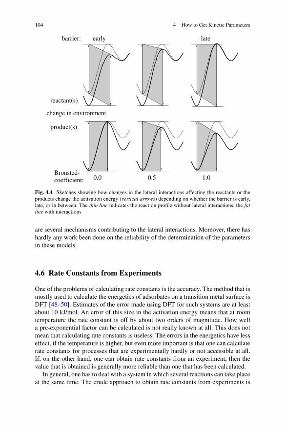
104 4 How to Get Kinetic Parameters

Fig. 4.4 Sketches showing how changes in the lateral interactions affecting the reactants or theproducts change the activation energy (vertical arrows) depending on whether the barrier is early,late, or in between. The thin line indicates the reaction profile without lateral interactions, the fatline with interactions

are several mechanisms contributing to the lateral interactions. Moreover, there hashardly any work been done on the reliability of the determination of the parametersin these models.

4.6 Rate Constants from Experiments

One of the problems of calculating rate constants is the accuracy. The method that ismostly used to calculate the energetics of adsorbates on a transition metal surface isDFT [48–50]. Estimates of the error made using DFT for such systems are at leastabout 10 kJ/mol. An error of this size in the activation energy means that at roomtemperature the rate constant is off by about two orders of magnitude. How wella pre-exponential factor can be calculated is not really known at all. This does notmean that calculating rate constants is useless. The errors in the energetics have lesseffect, if the temperature is higher, but even more important is that one can calculaterate constants for processes that are experimentally hardly or not accessible at all.If, on the other hand, one can obtain rate constants from an experiment, then thevalue that is obtained is generally more reliable than one that has been calculated.

In general, one has to deal with a system in which several reactions can take placeat the same time. The crude approach to obtain rate constants from experiments is

4.6 Rate Constants from Experiments 105

then to try to fit all rate constants to the experiments at the same time. This is seldoma good idea. First of all such a procedure can be quite complicated. The data thatone gets from an experiment are hardly ever a linear function of the rate constants.Consequently the fitting procedure consists of minimizing a nonlinear function thatstands for the difference between experimental and the calculated or simulated data.Such a function normally has many local minima, and it is very hard to find theglobal minimum. But this isn’t even the most important drawback. Although onemay be able to do a very good fit of the experimental data, this need not mean thatthe rate constants are good: they may be physically unrealistic, and given enough fitparameters, one can fit anything.

Deriving kinetic parameters from experiments does work well, when one hasan experiment of a single simple process that can be described by just one or twoparameters. The process should be simple in the sense that one has an analyticalexpression with which one can derive relatively easily the kinetic parameters giventhe experimental data. The analytical expression should be exact or at least a verygood approximation. If one has to deal with a reaction system that is complicatedand consists of many reactions, then one should try to get experiments that measurejust one of the reactions. For example, in CO oxidation one has at least adsorption ofCO, dissociative adsorption of oxygen, and the formation of CO2. Instead of tryingto fit rate constants of these three reactions simultaneously, one should look at ex-periments that show only one of these reactions. An experiment that only measuresadsorption as a function of CO pressure can be used to get the CO adsorption rateconstant. The following sections show a number of processes which can be used toget kinetic parameters, and we show how to get the parameters for these processes.

4.6.1 Relating Macroscopic Properties to Microscopic Processes

The analytical expressions mentioned above should relate some property that ismeasured to the rate constants. We will address first the general relation. This re-lation is exact, but rarely very useful. In the next sections we will show situationswere the general relation can be simplified either exactly or with the use of someapproximation.

If a system is in a well-defined configuration then a macroscopic property can ingeneral be computed easily. For example, the number of molecules of a particulartype in the adlayer can be obtained simply be counting. If the property that we areinterested in is denoted by X, then its value when the system is in configuration α

is given by Xα . We look at the expectation value of X, which is given by

〈X〉 =∑

α

PαXα. (4.71)

Kinetic experiment measure changes, so we look at d〈X〉/dt . This is given by

d〈X〉dt

=∑

α

dPα

dtXα, (4.72)

106 4 How to Get Kinetic Parameters

because Xα is a property of a fixed configuration. We can remove the derivative ofthe probability using the master equation. This gives us

d〈X〉dt

=∑

αβ

[WαβPβ − WβαPα]Xα,

=∑

αβ

WαβPβ [Xα − Xβ ]. (4.73)

The second step is obtained by swapping the summation indices. The final resultcan be regarded as the expectation value of the change of X in the process β → α

times the rate constant of that process. Equation (4.73) is called the phenomenolog-ical or macroscopic equation [51]. It forms the basis for deriving relations betweenmacroscopic properties and rate constants.

4.6.2 Simple Desorption

Suppose we have an atom or a molecule that adsorbs onto one particular type ofsite. We assume that we have a surface of area A with S adsorption sites. If Nα isthe number of atoms/molecules in configuration α then

d〈N〉dt

=∑

αβ

WαβPβ [Nα − Nβ ]. (4.74)

Diffusion does not change the number of atoms/molecules, and it does not matter inthis case whether we include it or not. The only relevant process that we have to lookat is desorption. We mentally fix configuration β and look only at the summationover α. We have to distinguish between two types of terms: the ones where α canoriginate from β by a desorption, and the ones where it cannot. The latter termshave Wαβ = 0, because there is no process that changes β into α, and so they donot contribute to the sum. The former do contribute and we have Wαβ = Wdes, withWdes the rate constant for desorption. We also have in this case Nα − Nβ = −1,because desorption removes one atom/molecule from the surface. So all these non-zero terms contribute the same value −Wdes to the sum for a given configuration β .Moreover, the number of these terms is equally to the number of atoms/moleculesin β that can desorb, because each desorbing atom/molecule yields a different α.This number of atoms/molecules is Nβ , so

d〈N〉dt

= −Wdes

∑

β

PβNβ = −Wdes〈N〉. (4.75)

This is an exact expression. Dividing by the number of sites S gives the rate equationfor the coverage θ = 〈N〉/S.

dθ

dt= −Wdesθ. (4.76)

4.6 Rate Constants from Experiments 107

If we compare this to the macroscopic rate equation dθ/dt = −kdesθ with kdes themacroscopic rate constant, we see that kdes = Wdes.

For isothermal desorption kdes does not depend on time and the solution to therate equation is

θ(t) = θ(0) exp[−kdest], (4.77)

where θ(0) is the coverage at time t = 0. Kinetic experiments often measure rates,and for the desorption rate we have

dθ

dt(t) = −kdesθ(0) exp[−kdest]. (4.78)

We can now obtain the rate constant by measuring, for example, the rate of desorp-tion as a function of time and plotting minus the logarithm of the rate as a functionof time. Because

ln

[−dθ

dt(t)

]= ln

[kdesθ(0)

]− kdest, (4.79)

we can obtain the rate constant which equals minus the slope of the straight line.The same would hold if we would plot the logarithm of the coverage as a functionof time. Because of the equality this immediately also yields the rate constant Wdesto be used in a simulation.

If the rate constant depends on time then solving the rate equation is often muchmore difficult. We can always rewrite the rate equation as

1

θ

dθ

dt= d ln θ

dt= −kdes. (4.80)

Integrating this equation yields

ln θ(t) − ln θ(0) = −∫ t

0dt ′kdes

(t ′), (4.81)

or

θ(t) = θ(0) exp

[−∫ t

0dt ′kdes

(t ′)]

. (4.82)

Whether of not we can get an analytical solution depends on whether we can deter-mine the integral. In TPD experiments we have

kdes(t) = ν exp

[− Eact

kB(T0 + Bt)

](4.83)

with Eact an activation energy, ν a pre-exponential factor, kB the Boltzmann-factor,T0 the temperature at time t = 0, and B the heating rate. The integral can be calcu-lated analytically. The result is

∫ t

0dt ′ν exp

[− Eact

kB(T0 + Bt ′)

]= Ω(t) − Ω(0) (4.84)

with

Ω(t) = ν

B(T0 + Bt)E2

[Eact

kB(T0 + Bt)

], (4.85)

108 4 How to Get Kinetic Parameters

where E2 is an exponential integral [11]. Although this solution has been derivedsome time ago [52], it has not yet been used in the analysis of experimental spectra,but there are several numerical techniques that work well for such simple desorption[53]. Note that we have not made any approximations here and the rate constant Wdesthat we obtain will be exact except for experimental errors.

4.6.3 Simple Adsorption

We start with the simplest case in which the adsorption rate is proportional to thenumber of vacant sites, which is called Langmuir adsorption. We will only indicatein this section in what way the common situation in which the adsorption is higherthan expected based on the number of vacant sites differs [2, 54, 55]. This so-calledprecursor-mediated adsorption is really a composite process.

Again suppose we have atoms or molecules that adsorb onto one particular typeof site. We assume that we have a surface of area A with S adsorption sites. If Nα isthe number of atoms/molecules in configuration α then again

d〈N〉dt

=∑

αβ

WαβPβ [Nα − Nβ ]. (4.86)

Diffusion can again be ignored as for desorption (see Sect. 4.6.2). For the summationover α we have to distinguish between two types of terms: the ones in which α canoriginate from β by a adsorption, and the ones it cannot. The latter terms haveWαβ = 0 and so they do not contribute to the sum. The former do contribute andwe have Wαβ = Wads, with Wads the rate constant for adsorption, and Nα − Nβ = 1,because adsorption adds one atom or molecule to the surface. So all these non-zero terms contribute equally to the sum for a given configuration β . Moreover, thenumber of these terms is equal to the number of vacant sites in β onto which themolecules can adsorb, because each adsorption yields a different α. The number ofvacant sites in configuration β equals S − Nβ , so

d〈N〉dt

= Wads

∑

β

Pβ(S − Nβ) = Wads(S − 〈N〉). (4.87)

Dividing by the number of sites S gives the rate equation for the coverage θ =〈N〉/S.

dθ

dt= −Wads(1 − θ). (4.88)

If we compare this to the macroscopic rate equation dθ/dt = kads(1 − θ) with kadsthe macroscopic rate constant, we see that kads = Wads.

So far adsorption is almost the same as desorption. The only difference is wherewe had θ for desorption we have 1 − θ for adsorption on the right-hand-side ofthe rate equation. An important difference now arises however. Whereas the macro-scopic rate constant for desorption kdes is an basic quantity in kinetics of surface

4.6 Rate Constants from Experiments 109

reactions, kads is generally related to other properties. This is because the adsorp-tion process consists of atoms or molecules impinging on the surface, and that issomething that can be described very well with kinetic gas theory.

Suppose that the pressure of the gas is P and its temperature T , then the numberof molecules F hitting a surface of unit area per unit time is given by [7, 56]

F = P√2πmkBT

(4.89)

with m the mass of the atom or molecule. Not every atom or molecule that hitsa surface will stick to it. The sticking coefficient σ is defined as the ratio of thenumber of molecules that stick to the total number hitting the surface. It can also belooked upon as the probability that an atom or molecule hitting the surface sticks.The change in the number of molecules in an area A due to adsorption can thenbe written as the vacant area times the flux F times the sticking coefficient σ . Thevacant area equals the area A times the fraction of sites in that area that is notoccupied. This all leads to

d〈N〉dt

= A(1 − θ)Fσ. (4.90)

If we compare this to the equations above we find

Wads = AFσ

S= PAsiteσ√

2πmkBT, (4.91)

where Asite is the area of a single site.Section 4.4.3 contains a discussion of the role of the sticking coefficient in the

calculation of adsorption rate constants. The remarks there are just as appropriatehere. In particular, whether or not the sticking coefficient is included in the expres-sions for the kMC rate constant depends on how adsorption, but also desorption (seeSect. 4.4.3), is defined.

Adsorption described so far is proportional to the number of vacant sites. Exper-iments measure the rate of adsorption and with the expressions derived above onecan calculate the microscopic rate constant Wads. However, it is often found thatthe rate of adsorption starts at a certain value for a bare surface and then hardlychanges when particles adsorb until the surface is almost completely covered whenit suddenly drops to zero. This behavior is generally explained by describing the ad-sorption as a composite process [2, 54, 55]. A molecule impinging unto the surfaceadsorbs with the probability σ when the site it hits is vacant just as before. How-ever, a molecule that hits a site that is already occupied need not be scattered. It canadsorb indirectly. It first adsorbs, with a certain probability, in a second adsorptionlayer. Then it starts to diffuse over the surface in this second layer. It can desorb at alater stage, or, and that’s the important part, it can encounter a vacant site and adsorbthere permanently. This last part can increase the adsorption rate substantially whenthere are already many sites occupied. The precise dependence of the adsorptionrate on the coverage θ is determined by the rate of diffusion, by the rate of adsorp-tion onto the second layer, and by the rate of desorption from the second layer. If

110 4 How to Get Kinetic Parameters

there are factors that affect the structure of the first adsorption layer, e.g. lateral in-teraction, then these too influence the adsorption rate. If the adsorption is not direct,one talks about a precursor mechanism. A precursor on top of an adsorbed particleis an extrinsic precursor. An intrinsic precursor can be found on top of a vacant site[57]. The precursor mechanism will not always be operative for a bare surface: i.e.,there is not always an intrinsic precursor. This means that we can use Eq. (4.91) ifwe take for σ the sticking coefficient for adsorption on a bare surface.

4.6.4 Unimolecular Reactions

With the knowledge of simple desorption and adsorption given above it is now easyto derive an expression for the rate constant Wuni for a unimolecular reaction in termof a macroscopic rate constant. In fact the derivation is exactly the same as for thedesorption. Desorption changes a site from A to ∗, whereas a unimolecular reactionchanges it to B. Replace ∗ by B in the expression for the desorption (and Wdes byWuni) and you have the correct expression. As the expression for desorption do notcontain a ∗, the procedure is trivial and we find Wuni = kuni where kuni is the rateconstant from the macroscopic rate equation.

4.6.5 Diffusion

We treat diffusion in kMC as any other process, but experimentally one doesn’tlook at changes in coverages but at displacements of atoms and molecules. We willtherefore also look here at how the position of a particle changes.

We assume that we have only one particle on the surface, so that the particle’smovement is not hindered by any other particle and the relation between the macro-scopic properties and the kMC rate constant is simple. In practice this means thatthe coverage should be low. We also assume that we have a square lattice with axisparallel to the x- and the y-axis and that the distance between lattice points is givenby a. We will later look at other lattices. If xα is the x-coordinate of the particle inconfiguration α, then

d〈x〉dt

=∑

αβ

WαβPβ [xα − xβ ]. (4.92)

The x-coordinate changes because the particle hops from one site to another. Whenit hops we have xα −xβ = a,−a, and 0 for a hop along the x-axis toward larger x, ahop along the x-axis toward smaller x, or a hop perpendicular to the x-axis, respec-tively. All these hops have a rate constant Whop and are equally likely. This meansd〈x〉/dt = 0. The same holds for the y-coordinate.

4.6 Rate Constants from Experiments 111

More useful is to look at the square of the coordinates. We then find

d〈x2〉dt

=∑

αβ

WαβPβ

[x2α − x2

β

]. (4.93)

Now we have x2α − x2

β = 2axβ + a2,−2axβ + a2, and 0, respectively. Because thehops are still equally likely, we have

d〈x2〉dt

= 2Whopa2. (4.94)

We find the same for the y-coordinate. The macroscopic equation for diffusion is

d〈x2 + y2〉dt

= 4D, (4.95)

with D the diffusion coefficient. From this we see that we have Whop = D/a2.On a hexagonal lattice a particle can hop in six different directions for which

xα − xβ = a, a/2,−a/2,−a,−a/2, and a/2 and yα − yβ = 0, a√

3/2, a√

3/2,0,

−a√

3/2, and −a√

3/2. From this we get again d〈x〉/dt = 0. For the squared dis-placement we find x2

α − x2β = 2axβ + a2, axβ + a2/4,−axβ + a2/4,−2axβ +

a2,−axβ + a2/4, axβ + a2/4. This yields again d〈x2〉/dt = 2Whopa2. We find

the same expression for the y-coordinate, so that also for a hexagonal latticeWhop = D/a2. The same expression holds for a trigonal lattice. The derivation isidentical to the ones for the square and hexagonal lattices.

4.6.6 Bimolecular Reactions

For all of the processes we have looked at so far it was possible to derive exactmacroscopic equations from the master equation. This is not the case for bimolec-ular reactions. Bimolecular reactions will give rise to an infinite hierarchy of exactmacroscopic rate equations. There are two bimolecular reactions we will consider:A + B and A + A. The problem we have mentioned above is the same for both re-actions, but there is a small difference in the derivation of a numerical factor in themacroscopic rate equation. We will start with the A + B reaction.

We look at the number of A’s. The expressions for the number of B’s can beobtained by replacing A’s by B’s and B’s by A’s in the following expressions. Wehave

d〈N(A)〉dt

=∑

αβ

WαβPβ

[N(A)

α − N(A)β

], (4.96)

where N(A)α stands for the number of A’s. We look at the summation over α and

mentally fix β . If α can originate from β by a A + B reaction, then Wαβ = Wrx,

otherwise Wαβ = 0. If such a reaction is possible, then N(A)α − N

(A)β = −1. The

112 4 How to Get Kinetic Parameters

problem now is with the number of configurations α that can be obtained from β bya reaction. This number is equal to the number of AB pairs N

(AB)β . This leads then

to

d〈N(A)〉dt

= −Wrx

∑

β

PβN(AB)β = −Wrx

⟨N(AB)

⟩. (4.97)

We get the same right-hand-side for the change in the number of B’s. We see thaton the right-hand-side we have obtained a quantity that we didn’t have before. Thismeans that the rate equations are not closed.

We can now proceed in two ways. The first is to write down rate equations forthe new quantity 〈N(AB)〉 and hope that this will lead to equations that are closed. Ifwe do this, we find that this will not happen. Instead we will get a right-hand-sidethat depends on the number of certain combinations of three particles. We can writedown rate equations for these as well, and hope that this will lead finally to a closedset of equations. But that too won’t happen. Proceeding by writing rate equationsfor the new quantities that we obtain will lead to an infinite hierarchy of equations[58–63].

The second way to proceed is to introduce an approximation that will make afinite set of these equations into a closed set. We can do this at different levels. Thecrudest approximation, and the one that will lead to the common macroscopic rateequations, is to approximate 〈N(AB)〉 in terms of 〈N(A)〉 and 〈N(B)〉. This actuallyturns out to involve two approximations. The first one is that we assume that thenumber of adsorbates are randomly distributed over the surface. In this case wehave N

(AB)β = ZN

(A)β [N(B)

β /(S − 1)], with Z the coordination number of the lattice:i.e., the number of nearest neighbors of a site. (Z = 4 for a square lattice, Z = 6 fora hexagonal lattice, and Z = 3 for a trigonal lattice.) The quantity between squarebrackets is the probability that a neighboring site of an A is occupied by a B. Thisapproximation is called the Mean Field Approximation (MFA) and leads to

d〈N(A)〉dt

= − Z

S − 1Wrx

∑

β

PβN(A)β N

(B)β = − Z

S − 1Wrx⟨N(A)N(B)

⟩. (4.98)

This is still not a closed expression. We have⟨N(A)N(B)

⟩= ⟨N(A)⟩⟨N(B)

⟩+ ⟨[N(A) − ⟨N(A)⟩][

N(B) − ⟨N(B)⟩]⟩

. (4.99)

The second term on the right stands for the correlation between fluctuations in thenumber of A’s and the number of B’s. In general this is not zero. Because the numberof A’s and B’s decrease simultaneously because of the reaction, this term is expectedto be positive. Fluctuations however decrease when the system size is increased. Inthe thermodynamic limit S → ∞ we can set it to zero. (Neglecting the fluctuationsis often included in MFA.) We then finally get

d〈N(A)〉dt

= −Z

SWrx⟨N(A)

⟩⟨N(B)

⟩(4.100)

4.6 Rate Constants from Experiments 113

with S − 1 replaced by S because S � 1. Dividing by the number of sites S leadsthen to

dθA

dt= −ZWrxθAθB. (4.101)

This should be compared to the macroscopic rate equation

dθA

dt= −krxθAθB. (4.102)

We see from this that we have Wrx = krx/Z, but only if the two approximations arevalid. This may not be the case when the adsorbates form some kind of structure(e.g. islands or a superstructure) or when the system is small (e.g. a small cluster ofmetal atoms) and the fluctuations are large.

The derivation for the A + A reaction is almost the same. We have

d〈N(A)〉dt

=∑

αβ

WαβPβ

[N(A)

α − N(A)β

]. (4.103)

If α can originate from β by a A+A reaction, then Wαβ = Wrx, otherwise Wαβ = 0.

If such a reaction is possible, then N(A)α − N

(A)β = −2, because now two A’s react.

The number of configurations α that can be obtained from β by a reaction is equalto the number of AA pairs N

(AA)β . This leads then to

d〈N(A)〉dt

= −2Wrx

∑

β

PβN(AA)β = −2Wrx

⟨N(AA)

⟩. (4.104)

If we do not want to get an infinite hierarchy of equations with rate equationsfor quantities of more and more A’s, we have to make an approximation again.We approximate 〈N(AA)〉 in terms of 〈N(A)〉. We first assume that the numberof adsorbates are randomly distributed over the surface. In this case we haveN

(AA)β = (1/2)ZN

(A)β [N(A)

β /S]. Note the factor 1/2 that avoids double countingof the number of AA pairs. The quantity between square brackets is the probabilitythat a neighboring site of an A is occupied by a A. We have immediately assumedhere that S � 1. This approximation leads to

d〈N(A)〉dt

= −Z

SWrx

∑

β

Pβ

(N

(A)β

)2 = −Z

SWrx⟨(N(A)

)2⟩. (4.105)

The factor 2 that we had previously has canceled against the factor 1/2 in the ex-pression for the number of AA pairs. To proceed we note that

⟨(N(A)

)2⟩= ⟨N(A)⟩2 + ⟨(N(A) − ⟨N(A)

⟩)2⟩. (4.106)

The second term on the right stands for the fluctuations in the number of A’s. Thisis clearly not zero, but positive. Setting it to zero is again the thermodynamic limit.We finally get

d〈N(A)〉dt

= −Z

SWrx⟨N(A)

⟩2. (4.107)

114 4 How to Get Kinetic Parameters

Dividing by the number of sites S leads then to

dθA

dt= −ZWrxθ

2A. (4.108)

This should be compared to the macroscopic rate equation

dθA

dt= −2krxθ

2A. (4.109)

Note that there is a factor 2 on the right-hand-side, which is used because a reactionremoves two A’s. We see from this that we have Wrx = 2krx/Z.

4.6.7 Dissociative Adsorption

We deal here with the quite common case of a molecule of the type B2 that adsorbsdissociatively on two neighboring sites. An example of such adsorption is oxygenadsorption on many transition metal surfaces. We will see this adsorption for exam-ple when we will discuss the Ziff–Gulari–Barshad model in Chap. 7. We will seehere that it is often convenient to look at limiting cases to derive an expression ofthe rate constant of adsorption.

We look at the number of B’s. We have again

d〈N(B)〉dt

=∑

αβ

WαβPβ

[N(B)

α − N(B)β

], (4.110)

where N(B)α stands for the number of B’s. If α can originate from β by an adsorption

reaction, then Wαβ = Wads, otherwise Wαβ = 0. If such a reaction is possible, then

N(B)α − N

(B)β = 2. The problem now is with the number of configurations α that can

be obtained from β by a reaction. This number is equal to the number of pairs ofneighboring vacant sites N

(∗∗)β . This leads then to

d〈N(B)〉dt

= 2Wads

∑

β

PβN(∗∗)β = 2Wads

⟨N(∗∗)

⟩. (4.111)

The right-hand-side can in general only be approximated, but such an approximationis not needed for the case of a bare surface. In that case we have N(∗∗) = ZS/2,where Z is the coordination number of the lattice and S the number of sites in thesystem. This leads to

d〈N(B)〉dt

= ZSWads. (4.112)

The change in the number of adsorbates for a bare surface is also equal to

d〈N(B)〉dt

= 2AFσ, (4.113)

4.6 Rate Constants from Experiments 115

where A is the area of the surface, F is the number of particles hitting a unit areaof the surface per unit time, and σ is the sticking coefficient. The factor 2 is due tothe fact that a molecule that adsorbs dissociatively yields two adsorbates. The fluxF we’ve seen before and is given by

F = P√2πmkBT

(4.114)

with P the pressure, T the temperature and m the mass of a molecule. This meansthat

d〈N(B)〉dt

= 2APσ√2πmkBT

. (4.115)

If we compare this with expression (4.112), we get

Wads = 2AsitePσ

Z√

2πmkBT(4.116)

with Asite the area of a single site. (See Sects. 4.4.3 and 4.6.3 for a discussion of therole of the sticking coefficient.)

4.6.8 A Brute-Force Approach

Because kMC can be derived from first-principles it is exact for a given model orset of processes. So if we know which processes take place in a system, we knowwhich lateral interactions are important, and we know the atomic structure of thesystem and which sites are relevant, then we can in principle determine all kineticparameters by fitting kMC simulations to the experimental results. In fact, it mighteven be possible to use this to compare models and decide which one is the betterone. Fitting kinetic parameters of different models and comparing the quality of thefits might allow us to choose between various candidate models.

There are however a number of pitfalls to this approach. Most of them are typicalfor fitting procedures but there is also one that has to do with the nature of kMCsimulations. General problems with the approach are the following. Fitting will en-tail minimizing a function that indicates how much the kMC and the experimentalresults differ. Such a function may have multiple minima. Often one wants to havethe global minimum, but it may be that such a minimum corresponds to kinetic pa-rameters that are unphysical (e.g., ridiculous values for interaction parameters ornegative activation energies). The fitting procedure should therefore be restrictedto those areas of the parameter space that correspond the acceptable values for thekinetic parameters.

Although a minimum of the fitting function may be mathematically well defined,it is not uncommon that the fitting function changes very little in certain directions.This means that the experimental results do not depend very much or not at allon one or more kinetic parameters or certain combinations of kinetic parameters.As a consequence such parameters can not be determined well and the value that

116 4 How to Get Kinetic Parameters

Fig. 4.5 The value of the fitting function as a function of the value of the lateral interaction (di-vided by kB in K) between CO molecules at top sites on Rh(100) at nearest neighbors-distances(left) and at next-nearest-neighbors distances (right). Each cross corresponds to a single set of ki-netic parameters for which kMC results have been compared to experimental TPD-spectra duringthe fitting procedure

the fitting procedure will give for them will be extremely sensitive to errors in theexperimental results.

kMC has on top of this the problem that it is a stochastic method. This means thatmany numerical methods can not be used, for example because they use derivativesor because they become unstable. So we need a method that does a global mini-mization in a restricted parameter space and that can handle noisy data. It shouldalso indicate when a parameter does not influence the quality of the fit so that itcan not be determined. If possible it should also be efficient so that the numberof simulations that need to be done is small. There are a number of methods thatcan be considered. Simulating annealing and computational evolution methods areprime candidates [64–69], but particle swarm optimization, memetic algorithms,tabu search, and possibly others might be useful as well [69, 70].

Differential evolution was used in a study to obtain kinetic parameters for desorp-tion of CO on Rh(100) at low coverages [71]. The prefactor, the activation energy,and lateral interactions at three different distances between the CO molecules weredetermined. Figure 4.5 shows how the quality of the fit (i.e., the fitting functionthat needs to be minimized) depends on the interaction between nearest- and next-nearest neighbors. Note that variations in the nearest-neighbor interaction affects thefit hardly at all. This is because this interaction is strongly repulsive. The coverage is

References 117

Fig. 4.6 Results of a fitting procedure to determine the kinetic parameters for desorption of COmolecules at top sites on Rh(100). Each cross corresponds to a single set of kinetic parameters forwhich kMC results have been compared to experimental TPD-spectra during the fitting procedureand for which the fitting function was less than 10. The 10-base logarithm of the prefactor (in 1/s)is plotted on the horizontal and the activation energy (divided by kB in K) is plotted on the verticalaxis

low so that the system can and does avoid it and it does therefore not affect the TPDspectra. The spectra do depend on the next-nearest-neighbor interaction, which isconsequently much better defined. Figure 4.6 shows the region in (prefactor, activa-tion energy) space for which the fitting function is less than 10. Note that this regionis very elongated. This means that there is a combination of these parameters that iswell defined and another one that is not. The one that is well defined turns out to bethe rate constant for desorption.

A follow-up study looked at higher coverages where some CO molecules notonly adsorbed at the preferred top but also at bridge sites and where there weremore relevant kinetic parameters [72]. This study showed that it is important tohave a good model for the interactions in a system to get meaningful values for theinteraction parameters. Although the model in this study had double the number ofkinetic parameters as the one for low coverages, and the experimental TPD spectracould reasonably well be reproduced, the values of the lateral interactions were quitedubious. More work on this way to use kMC simulations to get kinetic parametersis needed.

References

1. C.G.M. Hermse, F. Frechard, A.P. van Bavel, J.J. Lukkien, J.W. Niemantsverdriet, R.A. vanSanten, A.P.J. Jansen, J. Chem. Phys. 118, 7081 (2003)

2. R.A. van Santen, J.W. Niemantsverdriet, Chemical Kinetics and Catalysis (Plenum, New York,1995)

3. W.H. Press, B.P. Flannery, S.A. Teukolsky, W.T. Vetterling, Numerical Recipes. The Art ofScientific Computing (Cambridge University Press, Cambridge, 1989)

118 4 How to Get Kinetic Parameters

4. D.G. Truhlar, A.D. Isaacson, B.C. Garrett, in Theory of Chemical Reaction Dynamics, Part IV,ed. by M. Baer (CRC Press, Boca Raton, 1985), pp. 65–138

5. C.S. Tautermann, D.C. Clary, J. Chem. Phys. 122, 134702 (2005)6. C.S. Tautermann, D.C. Clary, Phys. Chem. Chem. Phys. 8, 1437 (2006)7. D.A. McQuarrie, Statistical Mechanics (Harper, New York, 1976)8. A. Messiah, Quantum Mechanics (North-Holland, Amsterdam, 1961)9. H. Goldstein, Classical Mechanics (Addison-Wesley, Amsterdam, 1981)

10. M.J. Frisch, G.W. Trucks, H.B. Schlegel, G.E. Scuseria, M.A. Robb, J.R. Cheeseman,J.A. Montgomery Jr., T. Vreven, K.N. Kudin, J.C. Burant, J.M. Millam, S.S. Iyengar,J. Tomasi, V. Barone, B. Mennucci, M. Cossi, G. Scalmani, N. Rega, G.A. Petersson,H. Nakatsuji, M. Hada, M. Ehara, K. Toyota, R. Fukuda, J. Hasegawa, M. Ishida, T. Naka-jima, Y. Honda, O. Kitao, H. Nakai, M. Klene, X. Li, J.E. Knox, H.P. Hratchian, J.B. Cross,C. Adamo, J. Jaramillo, R. Gomperts, R.E. Stratmann, O. Yazyev, A.J. Austin, R. Cammi,C. Pomelli, J.W. Ochterski, P.Y. Ayala, K. Morokuma, G.A. Voth, P. Salvador, J.J. Dannen-berg, V.G. Zakrzewski, S. Dapprich, A.D. Daniels, M.C. Strain, O. Farkas, D.K. Malick,A.D. Rabuck, K. Raghavachari, J.B. Foresman, J.V. Ortiz, Q. Cui, A.G. Baboul, S. Clifford,J. Cioslowski, B.B. Stefanov, G. Liu, A. Liashenko, P. Piskorz, I. Komaromi, R.L. Mar-tin, D.J. Fox, T. Keith, M.A. Al-Laham, C.Y. Peng, A. Nanayakkara, M. Challacombe,P.M.W. Gill, B. Johnson, W. Chen, M.W. Wong, C. Gonzalez, J.A. Pople, Gaussian 03, re-vision b.04. Gaussian, Inc., Pittsburgh, PA (2003)

11. M. Abramowitz, I.A. Stegun, Handbook of Mathematical Functions with Formulas, Graphs,and Mathematical Tables (Dover, New York, 1965)

12. A. Szabo, N.S. Ostlund, Modern Quantum Chemistry: Introduction to Advanced ElectronicStructure Theory (McGraw-Hill, New York, 1982)

13. D. Frenkel, B. Smit, Understanding Molecular Simulation: From Algorithms to Applications(Academic Press, London, 2001)

14. A.R. Leach, Molecular Modelling. Principles and Applications (Longman, Singapore, 1996)15. W. Koch, M.C. Holthausen, A Chemist’s Guide to Density Functional Theory (Wiley-VCH,

New York, 2000)16. C.J. Cramer, Essentials of Computational Chemistry (Wiley, Chichester, 2004)17. R.A. van Santen, M. Neurock, Molecular Heterogeneous Catalysis (Wiley-VCH, Weinheim,

2006)18. O. Trushin, A. Karim, A. Kara, T.S. Rahman, Phys. Rev. B 72, 115401 (2005)19. K. Sastry, D.D. Johnson, D.E. Goldberg, P. Bellon, Phys. Rev. B 72, 085438 (2005)20. N. Castin, L. Malerba, Nucl. Instrum. Methods Phys. Res., Sect. B, Beam Interact. Mater.

Atoms 267, 3148 (2009)21. G. Henkelman, H. Jónsson, J. Chem. Phys. 111, 7010 (1999)22. G. Henkelman, G. Jóhannesson, H. Jónsson, in Progress in Theoretical Chemistry and

Physics, ed. by S.D. Schwarts (Kluwer Academic, London, 2000)23. G. Mills, H. Jónsson, G.K. Schenter, Surf. Sci. 324, 305 (1995)24. C. Popa, W.K. Offermans, R.A. van Santen, A.P.J. Jansen, Phys. Rev. B 74, 155428 (2006)25. C. Popa, R.A. van Santen, A.P.J. Jansen, J. Phys. Chem. C 111, 9839 (2007)26. D. Curulla, A.P. van Bavel, J.W. Niemantsverdriet, ChemPhysChem 6, 473 (2005)27. A.P. van Bavel, Understanding and quantifying interactions between adsorbates: CO, NO, and

N- and O-atoms on Rh(100). Ph.D. thesis, Eindhoven University of Technology, Eindhoven(2005)

28. C. Popa, A.P. van Bavel, R.A. van Santen, C.F.J. Flipse, A.P.J. Jansen, Surf. Sci. 602, 2189(2008)

29. D.H. Wei, D.C. Skelton, S.D. Kevan, Surf. Sci. 381, 49 (1997)30. J.N. Murrell, S. Carter, P. Huxley, S.C. Farantos, A.J.C. Varandas, Molecular Potential Energy

Functions (Wiley-Interscience, Chichester, 1984)31. A. van der Walle, G. Ceder, J. Phase Equilibria 23, 348 (2002)32. V. Blum, A. Zunger, Phys. Rev. B 69, 020103(R) (2004)

References 119

33. A.P.J. Jansen, W.K. Offermans, in Computational Science and Its Applications—ICCSA-2005.LNCS, vol. 3480, ed. by O. Gervasi (Springer, Berlin, 2005)

34. C.G.M. Hermse, A.P.J. Jansen, in Catalysis, vol. 19, ed. by J.J. Spivey, K.M. Dooley (RoyalSociety of Chemistry, London, 2006)

35. Y. Zhang, V. Blum, K. Reuter, Phys. Rev. B 75, 235406 (2007)36. D.M. Hawkins, J. Chem. Inf. Comput. Sci. 44, 1 (2004)37. A.P.J. Jansen, C. Popa, Phys. Rev. B 78, 085404 (2008)38. N.A. Zarkevich, D.D. Johnson, Phys. Rev. Lett. 92, 255702 (2004)39. R. Drautz, A. Díaz-Ortiz, Phys. Rev. B 73, 224207 (2006)40. D.E. Nanu, Y. Deng, A.J. Böttger, Phys. Rev. B 74, 014113 (2006)41. T. Mueller, G. Ceder, Phys. Rev. B 80, 024103 (2009)42. E.T. Jaynes, G.L. Bretthorst, Probability Theory: The Logic of Science (Cambridge University

Press, Cambridge, 2003)43. A. Gelman, J.B. Carlin, H.S. Stern, D.B. Rubin, Bayesian Data Analysis (Chapman &

Hall/CRC, Boca Raton, 2003)44. D. Sivia, J. Skilling, Data Analysis: A Bayesian Tutorial (Oxford University Press, Oxford,

2006)45. B. Hammer, Phys. Rev. B 63, 205423 (2001)46. J.N. Brønsted, Chem. Rev. 5, 231 (1928)47. M.G. Evans, M. Polanyi, Trans. Faraday Soc. 34, 11 (1938)48. P. Hohenberg, W. Kohn, Phys. Rev. 136, B864 (1964)49. W. Kohn, L.S. Sham, Phys. Rev. 140, A1133 (1965)50. R.G. Parr, W. Yang, Density-Functional Theory of Atoms and Molecules (Oxford University

Press, New York, 1989)51. N.G. van Kampen, Stochastic Processes in Physics and Chemistry (North-Holland, Amster-

dam, 1981)52. A.P.J. Jansen, Comput. Phys. Commun. 86, 1 (1995)53. A.M. de Jong, J.W. Niemantsverdriet, Surf. Sci. 233, 355 (1990)54. J.M. Thomas, W.J. Thomas, Principles and Practice of Heterogeneous Catalysis (VCH, Wein-

heim, 1997)55. G.A. Somorjai, Introduction to Surface Chemistry and Catalysis (Wiley, Chichester, 1993)56. R. Becker, Theorie der Wärme (Springer, Berlin, 1985)57. A. Cassuto, D.A. King, Surf. Sci. 102, 388 (1981)58. V.P. Zhdanov, Elementary Physicochemical Processes on Solid Surfaces (Plenum, London,

1991)59. J. Mai, V.N. Kuzovkov, W. von Niessen, Phys. Rev. E 48, 1700 (1993)60. J. Mai, V.N. Kuzovkov, W. von Niessen, Physica A 203, 298 (1994)61. J. Mai, V.N. Kuzovkov, W. von Niessen, J. Chem. Phys. 100, 6073 (1994)62. E.A. Kotomin, V.N. Kuzovkov, Modern Aspects of Diffusion-Controlled Reactions: Coopera-

tive Phenomena in Bimolecular Processes (Elsevier, Amsterdam, 1996)63. O. Kortlüke, V.N. Kuzovkov, W. von Niessen, Chem. Phys. Lett. 275, 85 (1997)64. S. Kirkpatric, C.D. Gelatt Jr., M.P. Vecchi, Science 220, 671 (1983)65. D.A. Goldberg, Genetic Algorithms in Search, Optimization, and Machine Learning

(Addison-Wesley, Reading, 1989)66. H.P. Schwefel, Evolution and Optimum Seeking (Wiley, Chichester, 1995)67. Z. Michalewicz, Genetic Algorithms + Data Structures = Evolution Programs (Springer,

Berlin, 1999)68. W. Banzhaf, P. Nordin, R.E. Keller, F.D. Francone, Genetic Programming: An Introduction

(Morgan Kaufmann, San Francisco, 1998)69. D. Corne, M. Dorigo, F. Glover, New Ideas in Optimization (McGraw-Hill, London, 1999)70. E. Bonabeau, M. Doriga, G. Theraulaz, Swarm Intelligence: From Natural to Artificial Systems

(Oxford University Press, New York, 1999)71. A.P.J. Jansen, Phys. Rev. B 69, 035414 (2004)72. M.M.M. Jansen, C.G.M. Hermse, A.P.J. Jansen, Phys. Chem. Chem. Phys. 12, 8053 (2010)

Chapter 5Modeling Surface Reactions I

Abstract The main part of modeling surface reactions is concerned with the de-scription of the processes. For simple systems there is a lattice corresponding tothe adsorption sites and the labels of the lattice points describe the occupation ofthe sites. The labels can however also be used to model steps and other defects andsites on a bimetallic substrates. The lattice points need not necessarily correspondto sites, but can also be used to store other information like the presence of certainstructures in the adlayer. Processes need not always correspond to reactions or otheractual processes but when they have an infinite rate constant they can be used in ageneral-purpose code to handle exceptional situations that are normally hard-codedin special-purpose codes. Apart from implementing the processes, modeling alsoinvolves specifying system size, length of a simulation, and I/O. This is discussedin relation to reducing the noise in the output of a kinetic Monte Carlo simulation.

5.1 Introduction

In this chapter we will start looking at how to model surface processes. This mayseem rather trivial. One “just” has to specify which sites are involved in a process,and the occupation of these sites before and after the process. It turns out that thisis often indeed all one needs to do to simulate a system, but often there are var-ious ways to model a system, and then the question is which one gives the mostefficient simulation. This is typically the case when one has a system with differenttypes of site, processes with very different rate constants, diffusion, and/or lateralinteractions.

This chapter is particularly important for people using general-purpose codesto do kinetic Monte Carlo (kMC) simulations, because they have the opportunityto vary their model. If you use a special-purpose code then you do not have thatluxury. You are forced to use the model that is hard-coded. However, this chapter isalso relevant if you want to write such special-purpose codes, because there may bevarious ways your model can be coded.

The modeling framework that we present here is based on the assumption thata kMC code can recognize patterns in the occupation of sites, and that it can thenchange those patterns according to rules that stand for how processes change the site

A.P.J. Jansen, An Introduction to Kinetic Monte Carlo Simulations of SurfaceReactions, Lecture Notes in Physics 856,DOI 10.1007/978-3-642-29488-4_5, © Springer-Verlag Berlin Heidelberg 2012

121

122 5 Modeling Surface Reactions I

occupations. This framework is explained in Sect. 5.3, and how simple processes aremodeled with it in Sect. 5.4.

The framework however is much more flexible and powerful than the straightfor-ward implementation of simple processes. Section 5.5 shows how it can be used tomodel various types of substrate: e.g., multiple sites in the unit cell, steps and otherdefects, bimetallic surfaces, and reconstructions.

For some systems the pattern matching approach seems not to be appropriatehowever. For example, if we have a long reptating chainlike molecule, the numberof possible patterns or configurations of the molecule can simply be too large tospecify. In a special-purpose code this would be modeled by code that would firstmove the head of the molecule, then move along its length to find the tail, and finallymove the tail. We will show that we can do something similar within our frameworkwith so-called immediate processes. Such processes are also convenient for manyother situations. Some examples are shown in Sect. 5.6.

This chapter discusses only the components that can be used to model reactionsystems. It gives an overview of the tools that we can use in modeling reaction sys-tems with a general-purpose kMC code. It does not say anything about what wouldbe a good way to model certain processes. This is done in Chap. 6, which shows howthese tools can then be used to model specific processes in various ways. Chapter 7shows examples how reaction systems have actually been modeled. That chapterfocuses on the kind of kinetic information one can obtain from kMC simulations.

Apart from specifying the processes, to do a kMC simulation you also need tospecify other parameters like the size of the system that you want to simulate, thelength of the simulation, information on I/O, and possibly other things. We startthis chapter with a discussion of these other parameters and in particular on how todeal with the stochastic nature of kMC. We will see that there are different ways toreduce the noise that is intrinsic in the results of kMC simulations.

5.2 Reducing Noise

kMC is a stochastic method. This means that the results will show fluctuations andwill be noisy, and one often wants to do something to reduce the noise as it may beunacceptably large. This is often the case because one wants to simulate a surfacewith macroscopic dimensions, but one can only simulate much smaller systems. Inprinciple, there are three methods that one can use. We will discuss these methodsfor the Ziff–Gulari–Barshad (ZGB) model of CO oxidation and for Temperature-Programmed Desorption (TPD) spectra of simple desorption. Details of the ZGBmodel and its implementation can be found in Sect. 7.4.3. Section 5.4.1 has de-tails on TPD and simple desorption. These details are not relevant however for thediscussion here on noise reduction.

Figure 5.1 shows how the rate of CO2 production in kMC simulations of theZGB model changes if we average over several simulations. As the number of sim-ulations increases, the noise decreases. Because the simulations are independent of

5.2 Reducing Noise 123

Fig. 5.1 The reactivity (in reciprocal units of time) defined as the number of reactions formingCO2 per unit cell per unit of time as a function of time in the ZGB model. All simulations were donewith a square lattice with 128×128 lattice points and periodic boundary conditions. The parameterof the model was chosen to be y = 0.5255 which is about the value with maximum reactivity.This parameter stands for the fraction of molecules in the gas phase that are CO molecules and italso defines the unit of time as explained in Sect. 7.4.3. The numbers on the right of the curvesindicate the number of simulations over which the reactivity has been averaged. Only the curvewith the result from a single simulation shows the actual reactivity. Each other result has beenoffset vertically by an additional 0.03 reciprocal units of time. The inset shows a log-log plot ofthe noise, defined as the root-mean-square deviation of the reactivity, as a function as the numberof simulations that were used for the averaging. The points lie very close to a line with slope − 1

2

each other the noise is inverse proportional to the square root of the number of simu-lations. This way to reduce noise is straightforward. It only requires more computertime the smaller one wants the noise to be.

A second way to reduce noise is to increase the size of the system. That is shownin Fig. 5.2. The effect of this is the same as averaging over multiple simulations.Doubling the linear dimension of a system quadruples the number of sites and givesthe same result as averaging over four simulations with the original system size. Theonly difference may be that changing the system size may cost more computer time.For example, computer time per event in First Reaction Method increases slightlywith system size so doubling the linear dimension of a system costs more than fourtimes in computer time (see Sect. 3.5). For other algorithms that need not be thecase however.

Figure 5.2 also shows the noise in the coverage of CO. Oxygen shows the samevariation. We see that the noise in the coverage relative to the average coverage issomewhat larger than the noise in the reactivity relative to the average reactivity.

124 5 Modeling Surface Reactions I

Fig. 5.2 The reactivity (in reciprocal units of time) on the left, defined as the number of reactionsforming CO2 per unit cell per unit of time, and the coverage of CO on the right as a function oftime in the ZGB model. The parameter of the model was chosen to be y = 0.5255 which is aboutthe value with maximum reactivity. This parameter stands for the fraction of molecules in the gasphase that are CO molecules and it also defines the unit of time as explained in Sect. 7.4.3. Allsimulations were done with a square lattice with L × L lattice points with L given by the numberto the right of the curves and periodic boundary conditions. Only the curves for L = 16 show theactual reactivity and coverage. Each other result has been offset by an additional 0.03 reciprocalunits of time for the reactivity and by 0.1 ML for the coverage

This is not always the case. Figure 5.3 shows the desorption rate and the coveragefor various system sizes for TPD spectra of simple desorption. We see that the noisein the coverage is much less than the noise in the desorption rate.

Figure 5.4 shows a third way to reduce noise. Instead of averaging over simula-tion or larger areas one can also average over longer time intervals. The figures ofthe rates in this section show output at times tstart + nΔt with tstart the time at thestart of a simulation, Δt a time interval, and n a non-negative integer. The rate attime tstart + nΔt for a particular n is obtained by counting the number of processesthat have occurred between tstart + (n − 1)Δt and tstart + nΔt and then dividing bythe size of the system (i.e.: the number of unit cells) and by Δt . The number ofprocesses that occurs in an interval fluctuates but it is expected that the fluctuationrelative to the length of the interval becomes smaller. That is indeed what is seen inthe figure.

This last way to reduce noise is the cheapest as the system size can be keptrelatively small and only one simulation needs to be done. The drawback is thatthe amount of data is reduced by averaging over larger and larger intervals. Fora steady state this is no problem as for such a situation one is not interested in

5.3 A Modeling Framework 125

Fig. 5.3 The desorption rate (in 1/s) on the left and the coverage on the right as a function oftemperature (in K) for a TPD experiment with simple desorption. The activation energy for des-orption was 124.7 kJ/mol and the prefactor 1013 s−1. The heating rate was 2 K/s and the initialcoverage 1 ML. All simulations were done with a square lattice with L × L lattice points and pe-riodic boundary conditions with L given by the number to the right of the curves. Only the curvesfor L = 16 show the actual desorption rate and coverage. Each other result has been offset by anadditional 0.012 s−1 for the desorption rate and by 0.1 ML for the coverage

temporal fluctuations anyway and one might as well average over the whole lengthof a simulation. Note that we are using here the ergodic hypothesis or ergodicitytheorem [1]. It states that such average over time is the same as an average over manyidentical systems. Instead of taking a large time interval Δt for steady states to getaverage coverages and rates, it is also possible to use a small Δt and average overthe variations as a functions of time after a simulation has been done. This has theadvantage that the fluctuations can be used to derive error estimates of the averages.

It is important to realize that we only want to reduce noise if a single simulationshows noise and it is meant to model a system in which this noise is supposedto be absent. There are other situations. For example, if the system that we try tosimulate is small, then the coverages and rates may actually fluctuate. The noise in asimulation then represents these fluctuations, and we do not want to average [2, 3].

5.3 A Modeling Framework

An implementation of kMC has to have information on the sites of the system thatis being simulated and the occupation of these sites. The sites will most likely be

126 5 Modeling Surface Reactions I

Fig. 5.4 The reactivity (in reciprocal units of time) defined as the number of reactions formingCO2 per unit cell per unit of time as a function of time in the ZGB model. All simulations were donewith a square lattice with 128×128 lattice points and periodic boundary conditions. The parameterof the model was chosen to be y = 0.5255 which is about the value with maximum reactivity. Thisparameter stands for the fraction of molecules in the gas phase that are CO molecules and it alsodefines the unit of time as explained in Sect. 7.4.3. The numbers on the right of the curves indicatethe time interval Δt over which the reactivity was averaged. Only the curve with the result witha time interval of 1 time unit shows the actual reactivity. Each other result has been offset by anadditional 0.03 reciprocal units of time

implemented as some two-dimensional array of integers, characters, booleans, orstrings, which indicates the occupations. As a string can be used to represent aninteger, character, or boolean as well, we will use only strings here, but we will callthem labels from now on. Such labels have the advantage over integers, characters,and booleans that they can often be given values with a meaning that is obvious.

Apart from the occupation, other information on the sites may be useful as well.Such additional information we will also represent with a label. One may think thata real or floating-point numbers can be useful if one wants to model for examplea local temperature. However a continuous change of a property does not fit in thetheory as described in Chap. 2. If one wants to model a continuous property of asite, it will have to be discretized, and then a label can be used again.

Our framework has already been discussed briefly in Sects. 2.1.3 and 2.1.4. Wecan indicate a site by a triplet (n1, n2/s). This is the site at position x(s)

0 + n1a1 +n2a2 with a1 and a2 the primitive vectors of the lattice formed by the sites, andx(s)

0 is the position of site number s within a unit cell. If there is only one siteper unit cell, then the “s” can be left out, leaving us with (n1, n2). Adding a labelspecifies information on the site. This can most easily be seen using an example.With (0,0/0) : CO we mean that there is a CO molecule adsorbed at the site atposition x(0)

0 . Note however that the meaning of the label is up to the user. For

example, (1,2/0) : S may indicate a sulfur atom adsorbed on the site at x(0)0 + a1 +

5.3 A Modeling Framework 127

2a2, but that need not be the meaning of the label S at all. It may also be defined bya user to indicate a step site, or something entirely different.

The meaning of a label is really defined implicitly by the way it can change: i.e.,by the processes in which it plays a role. For example, if the label S above stands fora sulfur atom then there will probably be reactions between the sulfur atom and otheradsorbates, there will be hops from one site to another to model diffusion, et cetera.If S stands for a step site, then there are processes in which it becomes occupied, orit is converted into a terrace site when the substrate changes its structure, et cetera.We therefore need to look at how processes are implemented.

It is in this aspect that general-purpose and special-purpose codes differ most.The processes in a special-purpose code are hard code: i.e., how the occupations orother properties of the sites change is determined by the code. In a general-purposecode the processes are descriptions specified by the user on input that are interpretedby the program.

The way we do this here is as follows. Each process has to be specified as a listof sites involved in the process, the labels of the sites before, and the labels of thesites after the process has taken place. For example, in

(0,0), (1,0) : A B → ∗ ∗ (5.1)

an integer pair (n1, n2) indicates as before a unit cell, A and B are reactants, and ∗the product. This can be interpreted as an molecule A reacting with a molecule B ata neighboring site to the right to form AB which immediately desorbs leaving twovacant sites. This interpretation, however, is based on the meaning of the labels A,B, and ∗ as mentioned before.1

The indices specifying the unit cells are relative. The specification above standsnot just for a process at (0,0) and (1,0), but at (n1, n2) and (n1 +1, n2) for any pairof integers n1 and n2. Having more than one site per unit cell is also possible. Forexample in

(0,0/0), (0,0/1) : A B → ∗ ∗ (5.2)

the reaction takes place on two sites in the same unit cell. The integers after theslash indicate which sites are involved. Note that we do not make any assumptionson distances or angles. So

(0,0), (1,0) : A B → ∗ ∗ (5.3)

1The point that the meaning of the labels is up to the user can not be emphasized often enough.Suppose we model CO oxidation on some transition metal surface. Then (0,0), (1,0) : CO O →∗ ∗ can be interpreted as a CO2 formation reaction that is followed immediately by desorp-tion of CO2 leaving two vacant sites. This interpretation is obvious as is the interpretation of(0,0), (1,0) : carbonmonoxide oxygenatom → vacant vacant for the same process. However, wemay also have (0,0), (1,0) : vase gravity → shard shard. This is just as correct, although of course,very misleading. For more complicated models the interpretation and the choice of meaningfullabels is not always straightforward. For a kMC simulation only the way labels can change asspecified by the processes and the rates with which these changes occur is what counts.

128 5 Modeling Surface Reactions I

may refer to a square, a hexagonal, or any other type of lattice. This too isimplicit in the reactions. If (0,0), (1,0) : A B → ∗ ∗ stands for a reaction ona square lattice, then there should also be reactions (0,0), (0,1) : A B → ∗ ∗,(0,0), (−1,0) : A B → ∗ ∗, and (0,0), (0,−1) : A B → ∗ ∗. If we have a hexag-onal lattice, then we should have the reaction specifications as for a square latticeplus (0,0), (1,1) : A B → ∗ ∗, and (0,0), (−1,−1) : A B → ∗ ∗ where we assumethat the angle between the primitive translations is 120◦.

Processes also have a reaction rate constant. That need not concern us here exceptthat for general-purpose codes it may be convenient to have the possibility of hav-ing processes with infinite rate constants. Such processes occur immediately whenthey become possible. We will call such processes immediate processes. In special-purpose codes immediate processes are often not regarded as processes at all, but assituations in which some special action needs to be taken. By extending our conceptof processes to these immediate processes, such situations need not be treated dif-ferently, and they fit neatly in the theoretical framework that we have described inChap. 2.

5.4 Modeling the Occupation of Sites

5.4.1 Simple Adsorption, Desorption, and UnimolecularConversion

Modeling simple adsorption, desorption, and unimolecular conversion is essentiallythe same. The essential part is that only one site is involved. In each case the processcan then be written as A → B. For adsorption A is a vacant site and B the siteoccupied by an adsorbate, for desorption A is the site occupied by an adsorbateand B a vacant site, and for conversion A is the adsorbate that is converted andB the adsorbate into which A is converted. Note that we only look at the site andits occupation. We ignore the fact that prior to adsorption the adsorbate is in the gasphase or dissolved in a solution. For the simulation this is irrelevant. In the followingwe use A → B as a generic form for all three cases.

Note that an Eley–Rideal reaction that takes place on a single site is also includedhere. If the product is a molecule that immediately desorbs, then A is an adsorbateand B is a vacant site. The reaction is then effectively the same as a desorption, butwith a rate constant that depends not only on temperature but also on the pressureof the gas-phase reactant. If the product stays on the surface at the same site as theadsorbed reactant, then B is the product. The reaction is then effectively the same asa conversion with the same caveat concerning the rate constant.

Modeling this reaction is very simple. In the notation of our framework (seeSect. 5.3) we have

(0,0) : A → B. (5.4)

5.4 Modeling the Occupation of Sites 129

Fig. 5.5 Change of the coverage (in ML: dashed curves) and the desorption rate (in reactions persecond per site: solid curves) as a function of time (in seconds) for isothermal (left) and tempera-ture-programmed (right) simple desorption. The lattice size in the kMC simulations was 128×128with periodic boundary conditions and each result is an average of 1000 simulations. The initialcoverage was 1 ML for all simulations. On the left the desorption rate constant is 0.4 s−1. On theright the activation energy is 124.7 kJ/mol, the prefactor is 1013 s−1, the heating rate is 2 K/s, andthe initial temperature is 350 K. The inset shows a snapshot of a simulation with a 64 × 64 squarelattice with the black circles depicting the adsorbates. It shows a situation in which about two thirdof the sites has been vacated

This means that for each lattice point that has a label A, this label can change to B.This is the whole specification of the process except for the rate constant.

Figure 5.5 shows a snapshot of a simulation of simple desorption. A square latticeis used, and about one third of the sites are occupied. Note that the adsorbates arerandomly distributed over the lattice. There is no mechanism that can lead to anykind of ordering. Figure 5.5 also shows how the coverage and the desorption ratechange in time. The coverage is given in monolayers (ML) which is the fractionof all sites that is occupied. For the isothermal desorption the coverage and thedesorption rate are simple exponential decreasing functions of time. For the TPDcase we have

θ(t) = θ(0) exp[Ω(0) − Ω(t)

](5.5)

as was shown in Sect. 4.6.2.

130 5 Modeling Surface Reactions I

5.4.2 Bimolecular Reactions and Diffusion

Bimolecular reactions are not really more difficult to model than processes involvingonly one site, but there are a few differences. The first one is that there are differentorientations that the reactants can have with respect to each other. One should alsobe aware that there is a difference if in A + B we have B = A or B = A. We havealready seen this difference in Sect. 4.6.6.

We start with the case with A + A and for simplicity we assume that we havea square lattice with periodic boundary conditions and that the A’s are adsorbatesthat react to form a molecule that immediately desorbs. So we have the associativedesorption 2A → 2∗. In our notation we get

(0,0), (1,0) : A A → ∗ ∗,

(0,0), (0,1) : A A → ∗ ∗.(5.6)

We see that we have to specify two ways in which the A’s can react correspondingto the different relative orientations of a pair of AA neighbors. Again we also haveto specify the rate constant.

Figure 5.6 show a snapshot of a simulation of such associative desorption. Wesee that we get isolated A’s. If we have no diffusion then these will remain on thesurface indefinitely. Figure 5.6 also shows how the coverage and the desorption ratechange in time.

If we include diffusion all the A’s will eventually react. Figure 5.7 shows thatindeed the coverage then goes to zero for large time t . We model the diffusion by

(0,0), (1,0) : A ∗ → ∗ A,

(0,0), (0,1) : A ∗ → ∗ A,

(0,0), (−1,0) : A ∗ → ∗ A,

(0,0), (0,−1) : A ∗ → ∗ A.

(5.7)

There are four processes because an A can hop to one of four neighboring sites ifvacant. If the diffusion is so fast that the particles are randomly mixed then we have

dθ

dt= −ZWdesθ

2. (5.8)

This was shown in Sect. 4.6.6. For the isothermal case this yields

θ(t) = θ(0)

1 + ZWdesθ(0)t, (5.9)

and for the TPD case

θ(t) = θ(0)

1 + Z[Ω(t) − Ω(0)]θ(0)(5.10)

5.4 Modeling the Occupation of Sites 131

Fig. 5.6 Change of the coverage (in ML: dashed curves) and the desorption rate (in reactionsper second per site: solid curves) as a function of time (in seconds) for isothermal (left) and tem-perature-programmed (right) associative desorption. The lattice size in the kMC simulations was128×128 with periodic boundary conditions and each result is an average of 1000 simulations. Theinitial coverage was 1 ML for all simulations. On the left the desorption rate constant is 0.4 s−1. Onthe right the activation energy is 124.7 kJ/mol, the prefactor is 1013 s−1, the heating rate is 2 K/s,and the initial temperature is 350 K. The inset shows a snapshot of a simulation with a 64 × 64square lattice with the black circles depicting the adsorbates. It shows a situation in which abouthalf of the sites has been vacated. We get horizontal and vertical rows of adsorbates, because theadsorbates desorb in pairs. Note that there is no diffusion in the simulations

with Ω given by Eq. (4.85). The coverages in Fig. 5.7 vary according to Eqs. (5.9)and (5.10) because the diffusion is fast.

Next we deal with the case with B = A and for simplicity we again assume thatwe have a square lattice with periodic boundary conditions and that A and B react toform a molecule that immediately desorbs so that we have the associative desorptionA + B → 2∗. We get

(0,0), (1,0) : A B → ∗ ∗,

(0,0), (0,1) : A B → ∗ ∗,

(0,0), (−1,0) : A B → ∗ ∗,

(0,0), (0,−1) : A B → ∗ ∗.

(5.11)

We see that we have to specify four ways in which an A can react with a B corre-sponding to the different relative orientations of a pair of AB neighbors. There aretwo more than for 2A → 2∗, because AB and BA are of course the same when A

132 5 Modeling Surface Reactions I

Fig. 5.7 Change of the coverage (in ML: dashed curves) and the desorption rate (in reactionsper second per site: solid curves) as a function of time (in seconds) for isothermal (left) and tem-perature-programmed (right) associative desorption with diffusion with a rate constant that is 100times the one of desorption. The lattice size in the kMC simulations was 128 × 128 with periodicboundary conditions and each result is an average of 1000 simulations. The initial coverage was1 ML for all simulations. On the left the desorption rate constant is 0.4 s−1. On the right the ac-tivation energy is 124.7 kJ/mol, the prefactor is 1013 s−1, the heating rate is 2 K/s, and the initialtemperature is 350 K

and B are the same. We can also include diffusion of A and B, which is modeled asin Eq. (5.7).

Figure 5.8 show a snapshot of a simulation of such a model. The initial config-uration corresponds to a random mixture of equal numbers of A’s and B’s. It canbe noted that there are areas that have almost no B’s and others that have almostno A’s. The reason is that locally the number of A’s and the number of B’s are notthe same. After some time the particles in the minority have reacted and the onlyparticles of the other type are left [4]. The size of the areas with only A’s or onlyB’s depends on the ratio between the rate constant of the reaction and the hoppingrate constant. This size increases as

√t with time [5]. Figure 5.8 also shows that the

coverages decrease as 1/√

t for large t [4, 6, 7]. Initially, however, the particles arestill randomly mixed, and the coverage decreases according to the macroscopic rateequations which yields θ(0)/[1 + ZWrxθ(0)t].

5.5 Modeling Adsorption Sites 133

Fig. 5.8 Change of the coverage (solid line) as a function of time (in seconds) for the reactionA + B → 2∗ on a 128 × 128 square lattice with periodic boundary conditions. The initial con-figuration was a fully occupied lattice with equal numbers of A’s and B’s. The rate constant forthe reaction is Wrx = 10 s−1 and for diffusion Whop = 1 s−1. The lower dashed line depicts thechange in coverage obtained from the macroscopic rate equations: i.e., when the adsorbates wouldbe randomly distributed at all times. The upper dashed line is proportional to t−1/2, and shows thedependence of the coverage at long times. The inset shows a snapshot of an area of 64 × 64 sitesat the end of the simulation. A’s are closed and B’s are open circles

5.5 Modeling Adsorption Sites

5.5.1 Using the Sublattice Index

The previous sections have shown how to model processes involving one or two siteson a surface with just one site per unit cell. If there is more than one site per unit cell,then we can use the third index in our notation to model the processes. Figure 5.9shows a (111) surface of an fcc metal (e.g., Pt). A study of the dehydrogenation ofNH3 on Pt(111) showed that NH3 prefers to adsorb at top sites, NH2 prefers bridgesites, NH and N prefer fcc sites, and H does not really have a preference [8, 9].To model the dehydrogenation of NH3 (NH3 → N2 + H2) we can choose primitivetranslations a1 and a2 making an angle of 60◦, the top site at 0 with index 0, the fccsite at 1

3 a1 + 13 a2 with index 1, the hcp site at 2

3 a1 + 23 a2 with index 2, the bridge

sites at 12 a1 with index 3, at 1

2 a2 with index 4, and at 12 a1 + 1

2 a2 with index 5. Thedehydrogenation can then be written as

(0,0/0), (−1,0/3), (0,0/1) : NH3 ∗ ∗ → ∗ NH2 H (5.12)

with ∗ a vacant site. We see that the site preference of the adsorbates necessitatesa process in which three sites are involved even though it is just a unimolecularreaction. This is quite usual for realistic models of reaction systems.

134 5 Modeling Surface Reactions I

Fig. 5.9 A (111) surface ofan fcc metal with top (black),hollow (gray), and bridgesites (white). The numbers arethe indices of the sites

In fact, the description misses an important aspect that increases the number ofsites substantially. With so many sites in the unit cell as in Fig. 5.9, the distancebetween the sites is quite small. As a consequence there is a very strong repulsionbetween adsorbates at two different sites in the unit cell. In fact, in the Density-Functional Theory study mentioned above it was found that the adsorbates did notstay at their preferred site during a geometry optimization when two of them wereplaced together in one unit cell [8, 9]. One way to deal with this is to say thatthis repulsion is so strong that an adsorbate at some site prevents other adsorbatesfrom occupying some of the neighboring sites. We can also say that these sites areblocked. For the dissociation of NH3 this means that it can only take place if thetarget sites for NH2 and H are not blocked. Suppose that an adsorbate blocks allsites within a circle with a radius equal to the lattice cell parameter of the substrate.The description above then has to be replaced by

(0,0/0), (−1,0/3), (0,0/1),

(−2,0/2), (−2,0/5), (−1,0/0), (−1,0/1), (−1,0/2), (−1,0/4), (−1,0/5),

(0,0/2), (0,0/3), (0,0/4), (0,0/5), (1,0/0), (1,0/4),

(−1,−1/1), (−1,−1/2), (−1,−1/4), (−1,−1/5),

(0,−1/1), (0,−1/2), (0,−1/4), (0,−1/5), (1,−1/4) :NH3 ∗ ∗ ∗ ∗ ∗ ∗ ∗ ∗ ∗ ∗ ∗ ∗ ∗ ∗ ∗ ∗ ∗ ∗ ∗ ∗ ∗ ∗ ∗ ∗→ ∗ NH2 H ∗ ∗ ∗ ∗ ∗ ∗ ∗ ∗ ∗ ∗ ∗ ∗ ∗ ∗ ∗ ∗ ∗ ∗ ∗ ∗ ∗ ∗ (5.13)

We see that only three sites actually change their occupation, but a further 22 haveto be included in the description to make sure that sites (−1,0/3) and (0,0/1) arenot blocked.

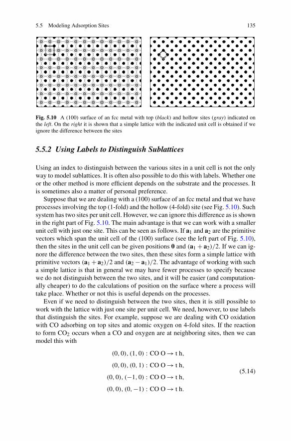
5.5 Modeling Adsorption Sites 135

Fig. 5.10 A (100) surface of an fcc metal with top (black) and hollow sites (gray) indicated onthe left. On the right it is shown that a simple lattice with the indicated unit cell is obtained if weignore the difference between the sites

5.5.2 Using Labels to Distinguish Sublattices

Using an index to distinguish between the various sites in a unit cell is not the onlyway to model sublattices. It is often also possible to do this with labels. Whether oneor the other method is more efficient depends on the substrate and the processes. Itis sometimes also a matter of personal preference.

Suppose that we are dealing with a (100) surface of an fcc metal and that we haveprocesses involving the top (1-fold) and the hollow (4-fold) site (see Fig. 5.10). Suchsystem has two sites per unit cell. However, we can ignore this difference as is shownin the right part of Fig. 5.10. The main advantage is that we can work with a smallerunit cell with just one site. This can be seen as follows. If a1 and a2 are the primitivevectors which span the unit cell of the (100) surface (see the left part of Fig. 5.10),then the sites in the unit cell can be given positions 0 and (a1 + a2)/2. If we can ig-nore the difference between the two sites, then these sites form a simple lattice withprimitive vectors (a1 + a2)/2 and (a2 − a1)/2. The advantage of working with sucha simple lattice is that in general we may have fewer processes to specify becausewe do not distinguish between the two sites, and it will be easier (and computation-ally cheaper) to do the calculations of position on the surface where a process willtake place. Whether or not this is useful depends on the processes.

Even if we need to distinguish between the two sites, then it is still possible towork with the lattice with just one site per unit cell. We need, however, to use labelsthat distinguish the sites. For example, suppose we are dealing with CO oxidationwith CO adsorbing on top sites and atomic oxygen on 4-fold sites. If the reactionto form CO2 occurs when a CO and oxygen are at neighboring sites, then we canmodel this with

(0,0), (1,0) : CO O → t h,

(0,0), (0,1) : CO O → t h,

(0,0), (−1,0) : CO O → t h,

(0,0), (0,−1) : CO O → t h.

(5.14)

136 5 Modeling Surface Reactions I

Here position (1,0) is at direction (a1 + a2)/2 from (0,0), whereas (0,1) is at di-rection (a2 − a1)/2 from (0,0). The labels “t” and “h” indicate a top or hollow site,respectively, being vacant. It is important to make sure that a “t” site is always asso-ciated with CO, and a “h” site always with oxygen. This means that CO adsorptionshould be modeled by

(0,0) : t → CO, (5.15)

and dissociative oxygen adsorption by

(0,0), (1,1) : h h → O O,

(0,0), (1,−1) : h h → O O.(5.16)

The relative positions (1,1) and (1,−1) here correspond to the translations a2 anda1, respectively. It is also important to make sure that the initial configuration cor-responds to a checkerboard pattern of “t” or CO and “h” or O. This kind of book-keeping has the obvious drawback of being error-prone.

With a unit cell with two sites we get for the CO adsorption

(0,0/0) : ∗ → CO, (5.17)

with the third “0” in (0,0/0) referring to the top site in the unit cell. The dissociativeadsorption of oxygen becomes

(0,0/1), (1,0/1) : ∗ ∗ → O O,

(0,0/1), (0,1/1) : ∗ ∗ → O O.(5.18)

The “1” in (0,0/1) indicates the hollow site. Note that we can now use the samelabel “∗” for any vacant site. The oxidation reaction becomes

(0,0/0), (0,0/1) : CO O → ∗ ∗,

(0,0/0), (−1,0/1) : CO O → ∗ ∗,

(0,0/0), (0,−1/1) : CO O → ∗ ∗,

(0,0/0), (−1,−1/1) : CO O → ∗ ∗.

(5.19)

Whether it is better to use labels to distinguish the sites or to work with a unit cellwith two sites depends on the processes and the substrate. Also coding may play arole. Calculations of the positions of where processes can take place can often bedone more efficient when the lattice sizes are powers of two using shift operators[10]. If we use labels, then this might not be possible. For example, suppose wehave a (111) surface of an fcc metal and we are dealing with top and the two hollowsites. These form again a simple lattice, but if we use this simple lattice and periodicboundary conditions then we have to work with system sizes that are multiples ofthree.

Sometimes extra sites need to be introduced if we want to use labels to distin-guish sublattices. Suppose that we have a (111) surface of an fcc metal. Suppose

5.5 Modeling Adsorption Sites 137

Fig. 5.11 A (111) surface of an fcc metal with only hollow sites indicated on the left. These sitesform a honeycomb lattice. If we add top sites we get a simple lattice as shown on the right

also that all adsorbates prefer the 3-fold sites: both the fcc and hcp sites. These sitestogether form the honeycomb structure shown in Fig. 5.11. If we ignore the differ-ence between the hcp and fcc sites, we do not get a simple lattice. So it seems notpossible to work with a smaller unit cell and use labels to distinguish between thesublattices. That impression is incorrect however.

The trick is to add sites to make a simple lattice. The right part of Fig. 5.11 showsthat if we add a site in the middle of each hexagon formed by the 3-fold sites, we doget a simple lattice. The extra site is at the position of a top site, but that is irrelevantas we will not use the site anyway. With the extra sites we can work with a smallerunit cell, but we need labels to distinguish between three types of sites.

It is clear that we are paying a price when we add extra sites. Although we do notuse them in the processes, we still need to store them. That price is however verymodest. It depends of course on the size of the system, but the number of sites rarelyexceeds 1 000 000, which means that our trick costs only a few Mb extra storage atmost.

5.5.3 Systems Without Translational Symmetry

The kMC simulations discussed here always assume that the sites form a lattice, butthis does not mean that we can only model systems with translational symmetry. Theprevious section on multiple sites in the unit cell has shown that by adding labelsspecifying extra properties of a site we can modify the lattice. We can use this tomodel a system without translational symmetry.

Suppose we want to model a stepped surface. We can model such a surface with alarge unit cell and multiple sites. This may not be a good idea, however. Suppose wehave parallel steps separated by wide terraces. We will then be dealing with a largeunit cell with many sites, and we will have to specify for each site its processes.This will generally lead to a long list of processes, even if the different sites on theterraces have the same properties, and only the sites at the steps behave differently.Moreover, we can not define such a unit cell if the width of the terraces varies. In

138 5 Modeling Surface Reactions I

such a case it is better to use a label to distinguish the sites at the step. For example,if we are dealing with simple desorption of an adsorbate A then we can modeldesorption from a terrace site as

(0,0) : A → ∗, (5.20)

and desorption from a site at the step as

(0,0) : As → ∗s. (5.21)

We add an “s” to indicate the adsorbate on a step site and a vacant step site. Notethat there is a difference with the example of CO oxidation on a (100) surface of thesection on multiple sites in Sect. 5.5.2. There the label “CO” already implied onetype of site and “O” another. Here the same adsorbate can be found on both typesof site. We also need to specify different rate constants for the desorption for bothtypes of site, because otherwise distinguishing them would not be meaningful. Theprecise position of the steps has to be specified in the initial configuration.

For a unimolecular reaction on a step we need to specify just two reactions. If wehave a bimolecular reaction we need to specify reactions for all possible combina-tions of occupations of step and terrace sites. So if we have a reaction A + B → 2∗,then we will have A B → ∗ ∗, As B → ∗s ∗, A Bs → ∗ ∗s, and As Bs → ∗s ∗s.Diffusion can also be regarded as a bimolecular reaction, and we need to spec-ify A ∗ → ∗ A, As ∗ → ∗s A, A ∗s → ∗ As, and As ∗s → ∗s As for the diffusionof A. Needless to say that all these possibilities will have in general different rateconstants.

In a realistic model of a surface it may not suffice to just change labels to indicatestep sites. Figure 5.12 shows a so-called (111) step of an fcc(111) surface. The figurealso shows the relevant sites if we assume that all adsorbates prefer top sites. If wedraw only the sites, we see that we have no translational symmetry in the directionperpendicular to the step. We can try to get translational symmetry by introducingextra sites as we have done with using labels to distinguish different sublattices (seeSect. 5.5.2). That is possible as is shown in the figure, but there is a much simplerapproach.

It is important to realize that the only geometric information that is used in kMCsimulations is the translational symmetry of the lattice points. There is no informa-tion on distances between the lattice points and their relative position with respectto each other. All that information is implicitly contained in the processes and theirrate constants. We have already seen that in the discussion of the modeling frame-work in Sect. 5.3 where we saw the difference in the associative desorption on asquare and a hexagonal lattice.

The relevance of these remarks on the geometric information is that we are al-lowed to shift sites and draw them as shown on the right in Fig. 5.12. We see thatwe have restored the translational symmetry in two directions. The way we can im-plement the step is now as follows. We label the sites at the step on the upper terraceusing “u” (for “up”), those at the step on the lower terrace using “d” (for “down”),and those on the terraces using “t” (for “terrace”). The processes use these labels to

5.5 Modeling Adsorption Sites 139

Fig. 5.12 A (111) step on a (111) surface of an fcc metal on the left, the top sites in the middle-left,top sites with extra sites in gray to form a simple lattice in the middle-right, and the simple latticethat is formed after the top sites of one terrace have been shifted on the right

Fig. 5.13 A (100) step on a (111) surface of an fcc metal on the left, the top sites in the middle,and the simple lattice that is formed after the top sites of one terrace have been shifted as indicatedby the arrow on the right

distinguish between terrace sites and those at the step just as before. That there is notranslational symmetry perpendicular to the step at the step is irrelevant.

Extra care is sometimes necessary. Figure 5.13 shows a (100) step of an fcc(111)surface. Again the top sites show only translational symmetry in two directions ifwe shift the sites of the upper terrace with respect to those of the lower terrace.But the shift is not perpendicular to the step in this case. There is also a compo-nent parallel to the step. This has two consequences. The first and most importantone has to do with the specification of the processes. Suppose we have a reactionbetween an adsorbate A at the bottom of the step and a neighboring adsorbate Bat the top of the step. This will give us a specification of the form Ad Bu → . . . ,where we have added “u” and “d” as defined above for a (111) step. The problemis the indexing of the sites. The right part of Fig. 5.13 suggests that we should have(0,0), (0,1) : Ad Bu → . . . and (0,0), (−1,1) : Ad Bu → . . . (a1 is then parallel tothe step and a2 makes an angle of 60◦ with a1), but the middle part of the figureclearly shows that a top site at the bottom of the step has only one top site as neigh-

140 5 Modeling Surface Reactions I

bor at the top of the step. One of these specification should therefore be left out. Itdepends on how we shift the sites which specification is the correct one to keep.

The second and more subtle consequence of the shift parallel to the step has todo with periodic boundary conditions. If we use the normal ones for the right part ofFig. 5.13, then we are effectively using skewed periodic boundary conditions for theactual system. As these conditions should not affect the results of the simulationsanyway, this does not matter for a proper simulation. It may matter however if wehave a system with a large correlation length. Suppose that we want to study areaction system that shows pattern formation (e.g., see Sect. 7.5.2). If the patternshave a length scale that is comparable to the size of the system, then the boundaryconditions can affect the results. Of course, one can argue that the system is thenchosen too small, but it may not be practical to increase the size of the system.

Using labels to indicate defects will be unavoidable if we have point defectsthat are not regularly distributed over the surface. The specification of the initialconfiguration determines where the defects are. It is of course also possible to havemore than one type of defect.

On a surface with defects most sites will be normal sites and only a minority willbe a defect site. Labels can also be used when that is not the case. This means thatwe can use it to model a surface of a bimetallic catalyst. Only the interpretation ofthe label changes: it will not indicate a normal or defect site, but a site on one or theother metal or even a site at the interface between the metals.

So far the occupation of the sites have been allowed to change through processes,but the properties of the sites themselves have been fixed. This need not be thecase. The surface composition of a bimetallic catalyst may change, or we might bedealing with a reconstructing surface. For a reconstructing surface we can introducea label that specifies to which phase of the substrate a site belongs. A change ofsurface composition of a bimetallic catalyst or a reconstruction can be modeledwith processes that specify the changes in the substrate. For example, there havebeen many studies of CO oxidation on reconstructing platinum surfaces. In one ofthe simplest models of this process there are process for the growth of the phases[11–13]. One phase, called the α phase, growths if there are no adsorbates. This canbe modeled by

(0,0), (1,0) : ∗α ∗ β → ∗α ∗ α. (5.22)

The β phase growths in an area with sites occupied by CO.

(0,0), (1,0) : COβ COα → COβ COβ. (5.23)

It should be realized that there are restrictions in what one can do with a changingsubstrate in kMC simulations. One does need to be able to put everything on alattice. Reconstructions that lead, for example, to surface structure with a differentdensity can only be modeled if this change is ignored [14]. Also it may not bepossible to model changes of the local point group symmetry.

5.5 Modeling Adsorption Sites 141

5.5.4 Bookkeeping Sites

All the lattices that we have seen so far correspond to the actual adsorption sites ofa substrate. That need not be. Often it is convenient to introduce an extra sublattice(i.e., extra sites in a unit cell) to store information. Suppose we have a Pt-Ru alloythat is used as an electrode for electrocatalytic CO oxidation [15, 16]. Also supposefor simplicity that the sites form a simple lattice, but some sites are on Pt and otherson Ru. We have CO and OH as adsorbates. The latter is formed when water disso-ciatively adsorbs. This forms OH on the electrode, a proton that dissolves, and anelectron that is taken up by the electrode. CO and OH react to form CO2 that desorbsimmediately, a proton, and an electron. To distinguish between adsorbates on Pt orRu we can use, for example, the labels CO(Pt), CO(Ru), OH(Pt), OH(Ru), ∗(Pt),and ∗(Ru) with obvious meaning. This would be the approach used in Sect. 5.5.3.

Another way to model this CO oxidation however is to use two sublattices or tohave two lattice points in the unit cell that both correspond to the same adsorptionsite. The idea of these two lattice points is that one has information on the occupation(CO, OH, or vacant) and the other on the metal of the substrate (Pt or Ru). Theformation of CO2 in the former approach would be represented by

(0,0), (1,0) : CO(Pt) OH(Ru) → ∗(Pt) ∗(Ru) (5.24)

and similar reactions. In the model with two sublattices this becomes

(0,0/0), (0,0/1), (1,0/0), (1,0/1) : CO Pt OH Ru → ∗ Pt ∗ Ru. (5.25)

The drawbacks of this approach are obvious. The description of the processes aremore extensive, and there is a higher memory use. The advantage is that the labelsbecome simpler, because we decouple the occupation from the type of site. Some-times it also makes the process description simpler. Suppose we have a diffusion ofCO that is the same on Pt and Ru. In such a case

(0,0/0), (1,0/0) : CO ∗ → ∗ CO (5.26)

is a good description. There is no reference to the substrate. This makes not only thedescription simpler, but it is also more efficient, because no checking is needed forthe labels of the other sublattice.

It is clear that splitting the information on a site over two or more sublatticescan also be used to model steps and reconstruction. But that is not the only waysuch extra lattice points can be used. We will see later that it can be convenient forstoring all kinds of useful information. This information can refer to one site or toa group of sites. We will call such extra lattice points bookkeeping sites, because ofthe nature of the information that is often stored in them.

142 5 Modeling Surface Reactions I

5.6 Using Immediate Processes

We have not given much attention in this chapter to the rate constants of the pro-cesses. We have only said that there is such a rate constant and from Chap. 3 weknow that this means that there is a probability distribution for the time that theprocess will take place. It turns out to be very convenient to allow the rate constantto become infinite and even to distinguish between different orders of infinity. Pro-cesses with an infinite rate constant occur immediately when they become possible(i.e., enabled in the terminology of Chap. 3) and we call them therefore immediateprocesses.

5.6.1 Very Fast Processes

The most trivial use of immediate processes is to model a very fast process: i.e., aprocess with a rate constant that is so large that it is almost certain that the processwill occur before any other process. In such a situation it is advantageous to use animmediate process. The first advantage is that one need not bother about determiningthe precise value of the rate constant. The second, and more important, advantageis that the time that the process occurs is the time that it has become possible, andno random number needs to be generated and a time determined. All computationsconcerning Eq. (3.11) or Eq. (3.25) are thus avoided.

There are many examples in the literature of such a use of immediate processes,in particular in studies of simple models directed at understanding certain kineticaspects and the development of kinetic concepts. For example, in the ZGB model(see Sect. 5.2) the formation of CO2 is assumed to be infinitely fast. This, and a fewother assumptions, allows the reduction of the number of kinetic parameters to justone: the fraction of gas molecules that are CO [17].

Using immediate processes does not mean that the generation of random num-bers is completely avoided for such processes. Suppose that in the ZGB model justmentioned a CO molecule adsorbs next to two oxygen atoms. Because CO2 forma-tion is an immediate process, CO will react with one of the oxygen atoms, but whichone is arbitrary and we need to generate a random number to decide which processwill actually take place.

Suppose that the CO molecule after adsorption could also react differently: e.g., itcould also dissociate. The question is then what the molecule will actually do. If theother process has a finite rate constant, then the immediate process (CO2 formation)will occur. But what if the other process is also an immediate process. For example,there is no CO diffusion in the original ZGB model, but diffusion is generally a veryfast process. So if we would have diffusion as an immediate process as well, thenthe situation is not clear. We might simply choose one of the processes, but that maybe unrealistic.

For such a case we distinguish between different orders of infinite rate constants:i.e., we give the immediate processes priorities. An immediate process with a high

5.6 Using Immediate Processes 143

Fig. 5.14 Snapshots of holes in an oxygen layer that have been formed from reactions with CO. Inboth cases the initial situation was a surface completely covered with oxygen except for one site.Diffusion of CO and reaction with oxygen are infinitely fast, but on the left the reaction is infinitelyfaster than the diffusion (i.e., it has a higher priority) and on the right it is the other way around

priority will occur before an immediate process with a low priority. This can beimportant. Figure 5.14 shows an oxygen layer that started with a small hole afterexposure to CO. CO adsorbs, reacts with oxygen possibly after diffusing over thesurface, and then forms CO2 which will desorb from the surface, thus enlarging thehole in the oxygen layer. The shape of the hole depends on whether diffusion orCO2 formation is the faster of the two processes.

The ZGB model uses a square lattice representing a (100) surface of an fcc metal.A CO molecule on such a lattice has a probability of reacting with a neighboringoxygen atom no matter on which neighboring site the oxygen atom sits. This shouldnot be the case for a rectangular lattice that represents a (110) surface of an fcc metal.There should be a different rate constant for a reaction with a neighboring oxygenatom in one direction than for the direction perpendicular to it. It is possible in thissituation too to have different priorities for the infinitely fast reactions. Supposea CO molecule has an oxygen atom neighbor in direction [1 1 0] and an oxygenatom neighbor in direction [1 0 0]. It will react with both of them infinitely fast, butit prefers to react with the one in direction [1 1 0] because it is nearer. In such asituation one should give the reaction with the neighbor in direction [1 1 0] a higherpriority.

5.6.2 Flagging Structural Elements

Very fast processes are certainly not the most important use of immediate processes.They are more important in situations where a special-purpose code would have apiece of code to handle special situations. We will show here that the same canoften be done with immediate processes. This has the advantage that the theoreticalframework of Chap. 2 still applies.

144 5 Modeling Surface Reactions I

As a first application we will look at using immediate processes to determinethe presence of certain structural elements. Suppose we do a simulation of Fischer–Tropsch synthesis [18]. The reaction conditions are such that chain growth is diffi-cult and we expect a high selectivity for methane and a rapidly decreasing amount ofCn species with increasing n. However, we find that hardly any methane is formed.The question is if this is due to the small rate constant of the CH3 + H → CH4 reac-tion, or if the diffusion of the reactants is hindered by a high coverage so much thatCH3 and H never meet.

There are various ways to answer that question, but we will look at one thatlooks at how often configurations in which the reactants can actually react occur. Ina special-purpose code this would be accomplished by code that would check thesystem by scanning the adlayer or by checking every time that a favorable configu-ration might have formed. Immediate processes do however as well. Apart from theprocesses we need bookkeeping sites to store information.

Let’s suppose for simplicity that we have a square lattice, and the CH4 can beformed if CH3 and H are at neighboring sites. For each pair of neighboring sites wecreate one bookkeeping site. Per unit cell we then have one real and two bookkeep-ing sites. Site (n1, n2/1) is the bookkeeping site for the pair of sites (n1, n2/0) and(n1 + 1, n2/0), and (n1, n2/2) for (n1, n2/0) and (n1, n2 + 1/0). The bookkeep-ing sites have a label “set” or “unset”. We start with all labels for the bookkeepingsites equal to “unset”. A site becomes “set” via one of the next immediate pro-cesses.

(0,0/0), (1,0/0), (0,0/1) : CH3 H unset → CH3 H set,

(0,0/0), (1,0/0), (0,0/1) : H CH3 unset → H CH3 set,

(0,0/0), (0,1/0), (0,0/2) : CH3 H unset → CH3 H set,

(0,0/0), (0,1/0), (0,0/2) : H CH3 unset → H CH3 set.

(5.27)

These processes allow us to determine the number of CH3–H pairs in a configura-tion.

The procedure above is all we need if we have a given configuration and want tocount the number of CH3–H pairs in that configuration. The immediate processesare then also the only processes that we need in a simulation: i.e., we have a separatesimulation for counting the number of CH3–H pairs. This is straightforward, but alsoquite cumbersome if we want to know how the number of CH3–H pairs varies in akMC simulation. What we rather have is a procedure that keeps track of the numberof CH3–H pairs during the Fischer–Tropsch simulation. For that we can still use theimmediate processes above, but we also need processes that unset the bookkeepingsites if processes occur that remove CH3–H pairs.

5.6 Using Immediate Processes 145

If we have only CH3 or H as adsorbates on the surface, then we only need

(0,0/0), (1,0/0), (0,0/1) : CH3 ∗ set → CH3 ∗ unset,

(0,0/0), (1,0/0), (0,0/1) : ∗ CH3 set → ∗ CH3 unset,

(0,0/0), (0,1/0), (0,0/2) : CH3 ∗ set → CH3 ∗ unset,

(0,0/0), (0,1/0), (0,0/2) : ∗ CH3 set → ∗ CH3 unset

(5.28)

where ∗ is a vacant site, to handle situations where hydrogen is removed from thesite. A similar set of immediate processes is needed for the case where CH3 isremoved. This method becomes rather cumbersome if CH3 or H can also react toform other adsorbates. For example, CH3 may split off another hydrogen atom andform CH2. We can of course extend the set of immediate processes, but anotherapproach may be easier.

We define another bookkeeping site (n1, n2/3). This site normally has a label“idle”. For each process that involves CH3 or H at site (n1, n2/0) the label of(n1, n2/3) is changed to “reset”. This triggers the following immediate processes,which change the older bookkeeping sites.

(0,0/3)(0,0/1) : reset set → reset unset,

(0,0/3)(0,0/2) : reset set → reset unset,

(0,0/3)(−1,0/1) : reset set → reset unset,

(0,0/3)(0,−1/2) : reset set → reset unset.

(5.29)

We don’t want the label of (n1, n2/3) to remain “reset” so we also need

(0,0/3) : reset → idle. (5.30)

This gives us all the necessary immediate processes, except that we also needsome control that makes sure that process (5.30) does not occur before all appropri-ate “set” labels are changed to “unset”. So as long as processes (5.29) are possible,process (5.30) should not take place. This can be accomplished by giving (5.29) ahigher priority than (5.30).

Suppose we have a process that swaps CH3 and H when they are neighbors. Wedo not want to change the “set” label corresponding to this pair, but because CH3and H might be part of other CH3–H pairs, we do change the “idle” labels of theseadsorbates to “reset”. This causes all neighboring “set” labels to “reset”, includingthe one of the CH3–H pair that is swapped. This is not what we want, but it is notreally a problem, because (5.27) changes it back to “set” again. However, this worksonly if (5.27) is the last immediate process to occur. So (5.27) should be given alower priority than (5.30) and (5.29).

We can now keep track of the number of CH3–H pairs in the Fischer–Tropschsimulation. There are two ways in which sublattices 1 and 2 can be used. One wayis simply to look at the “coverage” of the “set” labels. This is equal to the number

146 5 Modeling Surface Reactions I

of CH3–H pairs. This method might not work if this pairs exist only very brieflyand the labels of sublattices 1 and 2 are always all “unset”. It is then better to countthe number of times (5.27) occurs minus the number of times (5.29) occurs. Thereshould be no “set” labels in the initial configuration with this approach. This methodmay not work however if CH3–H pairs are very often formed and removed. Thereason is that one tries to determine a small difference between two large numbers,which is hard to do accurately.2

The method described above can be used to detect all other kind of structures.It can be transferred to the detection of any pair correlations as is, but also the wayto set up the detection of more complicated structures is straightforward. The ideais always to have an immediate process that is triggered when the structure that weare looking for is formed. This should change the label of a bookkeeping site. Thedifficult part is to change this label back when the structure is broken up. A carefulassignment of priorities is required as incorrect priorities can easily lead to infiniteloops of immediate processes.

5.6.3 Counting

Sometimes one wants to count how often some structural element is found at acertain position on the surface. This is really an extension of setting a flag to indicatethat a structural element is present or not. We will see in Sect. 6.3 how the result ofsuch counts can be used.

Suppose we have a site and we want to know how many of the neighboring sitesare occupied. For simplicity we assume that we have a square lattice and that thereis only one type of adsorbate which we call “A”. To store the count we need book-keeping sites: one for each real site. So we use a second sublattice. We need labelsthat indicate how many of the neighboring sites are occupied. It is natural to use thelabels “0”, “1”, “2”, “3”, and “4”. Note however that they look like integers, but inour formalism they are labels. In particular, we can not use them for arithmetic.

2Yet another way to determine the number of CH3–H pairs would be to have a normal processthat takes place if there is a CH3–H pair, but that does not change the configuration. The rateof such a process is equal to its rate constant times the coordination number of the lattice timesthe probability that a pair of neighboring sites is occupied by a CH3–H pair. As we know thecoordination number and can choose the rate constant, the rate allows us to calculate the probabilityof a CH3–H pair. This method has however one drawback. The result is approximate, becausethe process is a stochastic process. We can make the result more accurate by increasing the rateconstant, but that would increase the number of times that the process occurs and slow down thesimulation. The method with the immediate processes does not have this drawback, but it doesrequire more computer memory because of the bookkeeping sites and it is also more complex.

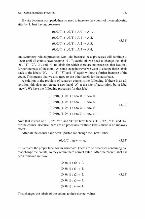
5.6 Using Immediate Processes 147

If a site becomes occupied, then we need to increase the counts of the neighboringsites by 1. Just having processes

(0,0/0), (1,0/1) : A 0 → A 1,

(0,0/0), (1,0/1) : A 1 → A 2,

(0,0/0), (1,0/1) : A 2 → A 3,

(0,0/0), (1,0/1) : A 3 → A 4,

(5.31)

and symmetry-related processes won’t do, because these processes will continue tooccur until all counts have become “4”. To avoid this we need to change the labels“0”, “1”, “2”, “3”, and “4” to labels for which there are no processes that lead to afurther increase of the count. At some stage however we want to change these labelsback to the labels “0”, “1”, “2”, “3”, and “4” again without a further increase of thecount. This means that we also need to use other labels for the adsorbate.

A solution to the problem of runaway counts is the following. If there is an ad-sorption, this does not create a new label “A” at the site of adsorption, but a label“new”. We have the following processes for that label.

(0,0/0), (1,0/1) : new 0 → new t1,

(0,0/0), (1,0/1) : new 1 → new t2,

(0,0/0), (1,0/1) : new 2 → new t3,

(0,0/0), (1,0/1) : new 3 → new t4.

(5.32)

Note that instead of “1”, “2”, “3”, and “4” we have labels “t1”, “t2”, “t3”, and “t4”for the counts. Because there are no processes for these labels, there is no runawayeffect.

After all the counts have been updated we change the “new” label.

(0,0/0) : new → A. (5.33)

This creates the proper label for an adsorbate. There are no processes containing “A”that change the counts, so they retain there correct value. After the “new” label hasbeen removed we have

(0,0/1) : t0 → 0,

(0,0/1) : t1 → 1,

(0,0/1) : t2 → 2,

(0,0/1) : t3 → 3,

(0,0/1) : t4 → 4.

(5.34)

This changes the labels of the counts to their correct values.

148 5 Modeling Surface Reactions I

Of course, the specification above calls for a specific order in which the processesshould occur. This means that these processes should all be immediate processeswith a certain priority. Processes (5.32) should have the highest priority, process(5.33) should have a lower priority, and processes (5.34) should have the lowestpriority.

In a similar way we can model desorption. The site from which an adsorbate hasjust desorbed gets a label “gone”. Then there is a set of processes with the samepriority as processes (5.32), which are giving by

(0,0/0), (1,0/1) : gone 1 → gone t0,

(0,0/0), (1,0/1) : gone 2 → gone t1,

(0,0/0), (1,0/1) : gone 3 → gone t2,

(0,0/0), (1,0/1) : gone 4 → gone t3.

(5.35)

Then there is

(0,0/0) : gone → ∗, (5.36)

with ∗ standing for a vacant site, which has the same priority as process (5.33).Finally, processes (5.34) occur which change the labels of the counts to their correctvalues.

Diffusion can be implemented using

(0,0/0), (1,0/0) : A ∗ → gone new, (5.37)

but note that this works for a square lattice, but not for an hexagonal lattice. Thereason why this works for a square lattice is that the neighbors of (0,0/0) and(1,0/0) form disjoint sets, and counts stored at (0,0/1) and (1,0/1) are handledcorrectly. If we have a hexagonal lattice, then there are two sites that are neighborsof both (0,0/0) and (1,0/0). The process above gives incorrect results for thesesites. The simplest way to handle this problem is to have an immediate processeslike

(0,0/0), (1,0/0), (1,1/1) : gone new 1 → gone new t1, (5.38)

et cetera with (1,1/1) a neighboring site of (0,0/0) and (1,0/0). This, and similarprocesses, should have a priority that is higher than any of the processes above.

Other processes that create or remove the adsorbate can be handled in the sameway. The approach can also be extended to systems with different types of adsorbate.

5.6.4 Decomposing the Implementation of Processes

When many sites are involved in a process they can be included directly in thedescription, but sometimes it is better to split it into a number of processes. Because

5.6 Using Immediate Processes 149

the combination of these processes must have a probability distribution for the timethat the process takes place that is the same of that of the description as a singleprocess, all but the first of these processes to occur must be immediate processes.This can be seen as follows. Suppose that we have just two processes with rateconstants W1 and W2. The process with rate constant W2 takes place after the onewith rate constant W1. If we start at time t = 0, then the second process will takeplace at a time t with probability distribution

∫ t

0dt ′W2e

−W2(t−t ′)W1e−W1t

′ = W1W2

W2 − W1

[e−W1t − e−W2t

]. (5.39)

This probability distribution differs from the usual exponential distribution unlessW1 or W2 is infinite. Because we want both processes to take place at the same time,we need W2 → ∞.

Suppose that we have an adsorbate A with a strong repulsion so that the neighbor-ing sites can not be occupied. There may be several reasons for this. The adsorbatemay be rather bulky, neighboring sites are very close, there is a strong through-metal interaction, et cetera [19]. We might try to model this using a description thatinvolves the adsorption site and its neighbors as is discussed in Sect. 6.2, but thereis another option. The adsorption we model simply with

(0,0) : ∗ → A (5.40)

with ∗ a vacant site. This process has a finite rate constant. The blocking of theneighboring sites is modeled with

(0,0), (1,0) : A ∗ → A blocked. (5.41)

This process, and the symmetry-related ones, are infinitely fast. This seems quitestraightforward, but things become a bit more tricky when the adsorbate can alsodiffuse and desorb. We look at desorption. Just

(0,0) : A → ∗ (5.42)

does not work, because this leaves “blocked” labels for sites that are not blockedany longer.

(0,0), (1,0) : A blocked → ∗ ∗ (5.43)

doesn’t work either, because this process can occur only once for each adsorbate.This means only one label “blocked” is changed back to ∗, but the adsorbate mayhave been blocking more than one site. What does work is first

(0,0) : A → vacated, (5.44)

The label “vacated” indicates that an adsorbate has just desorbed from the site. It isused to remove the “blocked” labels by

(0,0), (1,0) : vacated blocked → vacated ∗ (5.45)

150 5 Modeling Surface Reactions I

and symmetry-related immediate processes. Note that the label “vacated” stays sothat it can remove all “blocked” labels. To get rid of the “vacated” label we finallyhave another immediate process

(0,0) : vacated → ∗. (5.46)

It is clear that this process should only occur after all “blocked” labels have beenremoved, so it should have a lower priority than the previous process. The last thingthat we now need to do is to give the original blocking process (5.41) an even lowerpriority. If we would not do that we could get the following infinite loop

blocked A blocked A → blocked vacated blocked A→ blocked vacated ∗ A→ blocked vacated blocked A→ blocked vacated ∗ A→ . . . (5.47)

(We show only the sites along one line for convenience.) With the blocking processhaving the lowest priority, sites only become blocked again after the “vacated” labelhas been removed.

5.6.5 Implementing Procedures

The real strength of immediate processes becomes apparent when we model largemolecules with many configurations and possibly with different and/or variablesizes. For such systems it is not possible to list all patterns. Let’s assume we wantto model linear polymer chains on a surface. We assume that we can model suchmolecules with a square lattice with the monomers forming the polymer chains ad-sorbed on neighboring sites horizontally or vertically. Moreover, we assume thatmonomers that are not linked to each other can not be at neighboring sites eitherhorizontally, vertically, or diagonally. We show how immediate processes can beused to model reptation for such molecules.

We use three labels to model a polymer chain: “head”, “body”, and “tail” (seeFig. 5.15). The labels “head” and “tail” indicate the monomers at the ends. Theother monomers are labeled “body”. We will show how to implement a reptation“head”-first, but we will also show how to extend the model to have the polymerreptate in the opposite direction.

The first process, and the only one that is not an immediate process, moves thehead to a new position.

(0,1) (1,1)

(−1,0) (0,0) (1,0)

(0,−1) (1,−1)

:∗ ∗

head ∗ ∗∗ ∗

→∗ ∗

fh head ∗∗ ∗

. (5.48)

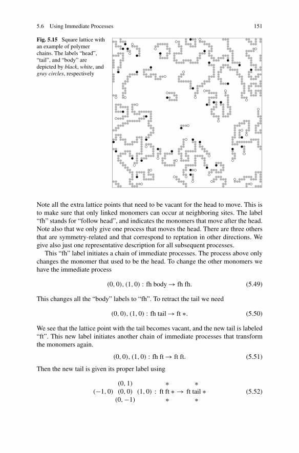
5.6 Using Immediate Processes 151

Fig. 5.15 Square lattice withan example of polymerchains. The labels “head”,“tail”, and “body” aredepicted by black, white, andgray circles, respectively

Note all the extra lattice points that need to be vacant for the head to move. This isto make sure that only linked monomers can occur at neighboring sites. The label“fh” stands for “follow head”, and indicates the monomers that move after the head.Note also that we only give one process that moves the head. There are three othersthat are symmetry-related and that correspond to reptation in other directions. Wegive also just one representative description for all subsequent processes.

This “fh” label initiates a chain of immediate processes. The process above onlychanges the monomer that used to be the head. To change the other monomers wehave the immediate process

(0,0), (1,0) : fh body → fh fh. (5.49)

This changes all the “body” labels to “fh”. To retract the tail we need

(0,0), (1,0) : fh tail → ft ∗. (5.50)

We see that the lattice point with the tail becomes vacant, and the new tail is labeled“ft”. This new label initiates another chain of immediate processes that transformthe monomers again.

(0,0), (1,0) : fh ft → ft ft. (5.51)

Then the new tail is given its proper label using

(0,1)

(−1,0) (0,0) (1,0)

(0,−1)

:∗

ft ft ∗∗

→∗

ft tail ∗∗

(5.52)

152 5 Modeling Surface Reactions I

and the rest of the monomer are changed to “body” using

(0,0) : ft → body. (5.53)

Note that (5.52) needs all the vacant lattice points to detect the proper “ft” label thatis the new tail.

It might seem that the combination of immediate processes is needlessly com-plicated, but it is not. In fact, these process as they stand are not complete yet. It isvery important to give them the correct priorities. The reason why there are so manyimmediate processes is that we want the changes that they make to occur in the sameorder that we have described them. What would definitely not work is moving thehead with (5.48) and the tail with

(0,0), (1,0) : body tail → tail ∗. (5.54)

The problem with this is that the processes are not coupled. We would then have oneprocess that elongates a polymer chain and another that shortens it but they can takeplace at different times and for different molecules. This would not be a reptation ofone polymer. The need for (5.49) is that we want to determine the tail of the samepolymer for which we move the head.

To see why we need (5.50) and (5.51) is more subtle. Why not have

(0,0), (1,0) : fh tail → tail ∗ (5.55)

instead of (5.50) and

(0,0) : fb → body ? (5.56)

The problem with this is that we get an infinite loop of immediate processes. As soonas the last process takes place, process (5.49) becomes possible again and changes“body” back to “fb”. The reason for changing “fb” to “ft” is to avoid such infiniteloops.

For processes (5.48) to (5.53) to work we need to assign priorities to avoid thesame kind of infinite loop. This means that we should not change “ft” too soon to“body”. Changing “fh” to “ft”, process (5.51), and making the new tail, process(5.52), should have a higher priority than the other processes. However, (5.51) and(5.52) can be given the same priority, and also the other processes can be given thesame, but lower, priority. Note that although some processes need to occur beforeothers, this does not necessarily imply that they need to have a higher priority. Forexample, (5.50) will always occur after (5.49) independent on the priorities.

The implementation above distinguishes between the two ends of the polymer,and reptation is only possible in one direction. If you want the polymer to reptatein both directions there are at least two possibilities. The easiest is to add a set ofprocesses that is identical to the ones above except that the roles of “head” and “tail”are reversed. (The names “head” and “tail” are then not appropriate anymore, andshould be changed.) It is advisable not to use “fh” and “ft” again, however, but useother labels. This is to avoid triggering any of the processes above.

References 153

The alternative is to add a set of processes that swap the labels “head” and “tail”.The drawback of this approach is that reptation in the opposite direction becomesa combination of two processes. This makes it slower and the distribution functionfor the time of occurrence is not an exponential function anymore (see Eq. (5.39)).

References

1. D.A. McQuarrie, Statistical Mechanics (Harper, New York, 1976)2. D.T. Gillespie, J. Comput. Phys. 22, 403 (1976)3. D.T. Gillespie, J. Phys. Chem. 81, 2340 (1977)4. V. Privman, Nonequilibrium Statistical Mechanics in One Dimension (Cambridge University

Press, Cambridge, 1997)5. S. Redner, in Nonequilibrium Statistical Mechanics in One Dimension, ed. by V. Privman

(Cambridge University Press, Cambridge, 1996), pp. 3–276. A.A. Ovchinnikov, Y.B. Zeldovich, Chem. Phys. 28, 215 (1978)7. D. Toussaint, F. Wilczek, J. Chem. Phys. 78, 2642 (1983)8. W.K. Offermans, A.P.J. Jansen, R.A. van Santen, Surf. Sci. 600, 1714 (2006)9. W.K. Offermans, A.P.J. Jansen, R.A. van Santen, G. Novell-Leruth, J.M. Ricart, J. Pérez-

Ramirez, J. Phys. Chem. C 111, 17551 (2007)10. B. Stroustrup, The C++ Programming Language (Addison-Wesley, Reading, 1991)11. V.N. Kuzovkov, O. Kortlüke, W. von Niessen, Phys. Rev. Lett. 83, 1636 (1999)12. O. Kortlüke, V.N. Kuzovkov, W. von Niessen, Phys. Rev. Lett. 83, 3089 (1999)13. V.N. Kuzovkov, O. Kortlüke, W. von Niessen, Phys. Rev. E 66, 011603 (2002)14. R.J. Gelten, A.P.J. Jansen, R.A. van Santen, J.J. Lukkien, J.P.L. Segers, P.A.J. Hilbers,

J. Chem. Phys. 108, 5921 (1998)15. M.T.M. Koper, J.J. Lukkien, A.P.J. Jansen, R.A. van Santen, J. Phys. Chem. B 103, 5522

(1999)16. M.T.M. Koper, N.P. Lebedeva, C.G.M. Hermse, Faraday Discuss. 121, 301 (2002)17. R.M. Ziff, E. Gulari, Y. Barshad, Phys. Rev. Lett. 56, 2553 (1986)18. B.H. Davis, M.L. Occelli, Fischer–Tropsch Synthesis, Catalysts and Catalysis. Studies in Sur-

face Science and Catalysis, vol. 163 (Elsevier, Amsterdam, 2006)19. C.G.M. Hermse, A.P.J. Jansen, in Catalysis, vol. 19, ed. by J.J. Spivey, K.M. Dooley (Royal

Society of Chemistry, London, 2006)

Chapter 6Modeling Surface Reactions II

Abstract The way to model many processes for kinetic Monte Carlo simulationsis straightforward. There are however also processes that one encounters regularlyand for which there are more modeling options and for which the best is not alwaysclear. We discuss here several of them. We look at how to handle site blocking bylarge adsorbates and other cases with strong repulsion. We show several ways to im-plement finite lateral interactions. Fast diffusion and other fast processes are shownto be not necessarily a hindrance for efficient simulations. Some fast processes caneven be combined with slower processes in one effective process. Tagging adsor-bates is introduced to simulate isotope experiments and to obtain information ondiffusion. Our two-dimensional modeling framework is shown to be capable to dealwith simulating reactions on nanoparticles. Non-physical processes are shown to beuseful to create the initial configuration of a kinetic Monte Carlo simulation.

6.1 Introduction

Chapter 5 has introduced the tools that are available within the theoretical frame-work of Chap. 2 to model processes on surfaces. In this chapter we discuss howthese tools can be used to model specific chemical and physical aspects that onemeets when one starts implementing such processes. The distinction between thetopics discussed here and those in Chap. 5 are not completely unambiguous. Forexample, the discussion on how to implement multiple sites in the unit cell of a sur-face (Sect. 5.5.2) and the various ways to model steps (Sect. 5.5.3) would also fitwell in this chapter. The difference between the chapters is really a point of view.In Chap. 5 we discussed modeling tools and showed what could be done with them.Here we will start with the question of how to model some process and then showhow to do that.

This chapter is also mainly important if you are using a general-purpose codefor your kinetic Monte Carlo (kMC) simulations, but it also gives an impression ofthe various ways you can hardcode some model in special-purpose codes. In fact,because the starting point in this chapter is some chemical or physical problem, itbrings the fact that there are often several ways to implement a model better to thefore.

A.P.J. Jansen, An Introduction to Kinetic Monte Carlo Simulations of SurfaceReactions, Lecture Notes in Physics 856,DOI 10.1007/978-3-642-29488-4_6, © Springer-Verlag Berlin Heidelberg 2012

155

156 6 Modeling Surface Reactions II

6.2 Large Adsorbates and Strong Repulsion

Suppose that we have adsorption of a somewhat bulky adsorbate A. The adsorbateoccupies not only a particular site, but also makes it impossible for other adsor-bates to occupy neighboring sites. We have already seen how this can be done withinfinitely fast processes in Sect. 5.6.4. The adsorption we model simply with

(0,0) : ∗ → A (6.1)

with ∗ a vacant site. This process has a finite rate constant. The blocking of theneighboring sites is modeled with the immediate process

(0,0), (1,0) : A ∗ → A blocked, (6.2)

and symmetry-related processes. For desorption we have

(0,0) : A → vacated. (6.3)

The label “vacated” indicates that an adsorbate has just desorbed from the site. It isused to remove the “blocked” labels by

(0,0), (1,0) : vacated blocked → vacated ∗, (6.4)

which is an another immediate process. Note that the label “vacated” stays so thatit can remove all “blocked” labels. To get rid of the “vacated” label we finally haveyet another immediate process

(0,0) : vacated → ∗. (6.5)

These immediate processes should be given the right priorities as discussed inSect. 5.6.4: i.e., (6.4) should have the highest priority, (6.5) a lower one, and (6.2)should have the lowest.

We have to take care if we want to extend this approach to diffusion. We mighttry

(0,0), (1,0) : A blocked → vacated A. (6.6)

The “vacated” label removes the “blocked” labels for the neighbors of the old ad-sorption site of A. However, this is not always correct, because site (1,0) mighthave other A’s at neighboring sites besides the one originally at (0,0). The processwould then put two, or more, A’s at neighboring sites.

One way to deal with this is to check the neighboring sites of (1,0). If we have asquare lattice this might look as follows. Instead of the process above, we have

(1,1)

(0,0) (1,0) (2,0)

(1,−1)

:notA

A blocked notAnotA

→notA

vacated A notAnotA

. (6.7)

6.2 Large Adsorbates and Strong Repulsion 157

Here “notA” stands for either “blocked” or “∗”. So there are really eight differentprocesses, plus symmetry-related ones, that we have to include to model the diffu-sion in this way. An alternative approach would be to undo a diffusion process thatshould not have occurred. We do use (6.6), but also add the immediate process

(0,0), (1,0), (2,0) : vacated A A → A blocked A (6.8)

with a priority higher than any of the other immediate processes. This process putsthe A that has just jumped back on its original site when it gets another A as itsneighbor. We also need to add two more processes to test for A’s at sites (1,1) and(1,−1) instead of (2,0).

Of course, undoing a process is inefficient. There may also be an inefficiencyrelated to the “vacated” label. The “blocked” labels on neighbors of “vacated” arechanged to “∗”, but this is not always what we want, because these sites may beneighbors of other adsorbates. These adsorbates will change the appropriate “∗”labels back to “blocked”, but only after “vacated” has been changed to “∗”. For thisreason another way to model these processes might be considered.

The advantage of using immediate processes is that the number of sites involvedin the description of a process can be kept low. Pattern matching will be efficient.Another way to model the same processes above is to check always the neighborsof a site that becomes occupied. If we have a square lattice the adsorption becomes

(0,1)

(−1,0) (0,0) (1,0)

(0,−1)

:∗

∗ ∗ ∗∗

→∗

∗ A ∗∗

. (6.9)

The desorption is very simple, because it involves no changes in labels except toone of the adsorption site.

(0,0) : A → ∗. (6.10)

Diffusion is very similar to adsorption. We get

(0,1)

(−1,0) (0,0) (1,0)

(0,−1)

:∗

A ∗ ∗∗

→∗

∗ A ∗∗

(6.11)

for a square lattice. For diffusion there are three other symmetry-related processes.We see that with this approach we do not have immediate processes, but adsorptionand diffusion involve more than two sites. Note also that we need to specify explic-itly all neighbors of a site. The description of adsorption and diffusion would bedifferent for a hexagonal lattice.

Although we have started this section with stating that the adsorbate A is bulky,the descriptions above are also valid for other adsorbates that prevent neighbor-ing sites from becoming occupied. This is the case for example when an adsorbatechanges the electronic structure of the substrate in such a way that adsorption onneighboring sites becomes unfavorable. Other mechanisms might be operable as

158 6 Modeling Surface Reactions II

well: see [1]. Suppose that the adsorbate is really large and not only prevents otheradsorbates from occupying neighboring sites, but actually occupies not just one sitebut also the neighboring sites. The following implementation then seems obvious.For adsorption we use

(0,1)

(−1,0) (0,0) (1,0)

(0,−1)

:∗

∗ ∗ ∗∗

→A

A A AA

, (6.12)

for desorption

(0,1)

(−1,0) (0,0) (1,0)

(0,−1)

:A

A A AA

→∗

∗ ∗ ∗∗

, (6.13)

and for diffusion

(0,1) (1,1)

(−1,0) (0,0) (1,0) (2,0)

(0,−1) (1,−1)

:A ∗

A A A ∗A ∗

→∗ A

∗ A A A∗ A

. (6.14)

There is one big problem with this implementation, however, and if that problem issolved then there is still one important difference with the two preceding implemen-tations.

The big problem is that the implementation is incorrect. When several adsorbatesare located close to each other, it is no longer clear which label “A” belongs to whichadsorbate. This makes it possible that processes take place that involve some A’sfrom one adsorbate and some from another. This is obviously not what we want.We need to distinguish between the different parts of the adsorbate. The adsorptioncould for example be modeled by

(0,1)

(−1,0) (0,0) (1,0)

(0,−1)

:∗

∗ ∗ ∗∗

→a

a A aa

. (6.15)

An adsorbate is now well-defined, because it is an “A” surrounded by “a”’s.This implementation however is not equivalent to the previous two. Only neigh-

boring sites were blocked for adsorption in the previous two implementations, butin the last implementation more sites are blocked. This can most easily be seen fora square lattice. An adsorbate on site (0,0) blocks only sites (1,0), (0,1), (−1,0),and (0,−1) in the first two implementations. A site like (1,1) is available for ad-sorption. This is not the case in the last implementation. The reason is that an ad-sorbate at (1,1) in the last implementation would also occupy the neighboring sites,among them (1,0) and (0,1). But these are already occupied. In the first two imple-mentation the maximum coverage for a square lattice is 0.5 ML and the adlayer thenhas a translational symmetry given by the primitive vectors a(1,1) and a(1,−1)

with a the distance between neighboring sites. In last implementation the maximumcoverage for a square lattice is 0.2 ML and the adlayer then has a translational sym-metry given by the primitive vectors a(2,1) and a(1,−2) (see Fig. 6.1).

6.3 Lateral Interactions 159

Fig. 6.1 A square lattice with an adsorbate that blocks neighboring sites for adsorption (left) andan adsorbate that occupies a central site and the four neighboring sites (right). In both cases anadlayer is shown with a maximum coverage. The black circles show the adsorbates (left) or thecentral sites occupied by the adsorbates (right). The white circles indicate all other sites

6.3 Lateral Interactions

Lateral interactions are interactions between adsorbates. It has been well-known fora long time that these interactions lead to structured or ordered adlayers at low tem-peratures. The realization that the kinetics of surface reactions can be substantiallyaffected by these interactions even at high temperatures is more recent. Relativelylittle is known about the form of these interactions and even less about the strengthof them [1]. In this section we present a number of ways to implement these inter-actions. In all cases we assume that the lateral interactions are short range.

The most general method to model lateral interactions consists of specifying theprocess and the occupation of the sites that may have adsorbates that will affect theprocess. For example, if we have a simple desorption of an adsorbate A on a squarelattice with a rate constant that depends on the occupation of the four neighboringsites, then we have

(0,1)

(−1,0) (0,0) (1,0)

(0,−1)

:∗

∗ A ∗∗

→∗

∗ ∗ ∗∗

,

(0,1)

(−1,0) (0,0) (1,0)

(0,−1)

:∗

∗ A A∗

→∗

∗ ∗ A∗

,

(0,1)

(−1,0) (0,0) (1,0)

(0,−1)

:A

∗ A A∗

→A

∗ ∗ A∗

, (6.16)

160 6 Modeling Surface Reactions II

(0,1)

(−1,0) (0,0) (1,0)

(0,−1)

:∗

A A A∗

→∗

A ∗ A∗

,

(0,1)

(−1,0) (0,0) (1,0)

(0,−1)

:A

A A A∗

→A

A ∗ A∗

,

(0,1)

(−1,0) (0,0) (1,0)

(0,−1)

:A

A A AA

→A

A ∗ AA

,

and symmetry-related desorptions. Each of these processes can be given a differentrate constant (or activation energy and prefactor). By specifying all possible occu-pations of the neighboring sites explicitly any dependence of the lateral interactionson the occupation of neighboring sites can be modeled. The disadvantage shouldalso be clear. The list of processes can be quite long. With Z neighboring sites thatmay be occupied by an adsorbate affecting a process and A possible occupations ofeach of these sites (including no adsorbate) there are AZ processes to specify.

Suppose that the rate constant for the desorption above depends only on the num-ber of neighbors of the adsorbate that desorbs. This is for example the case if wehave only interactions between pairs of adsorbates that change the activation en-ergy: i.e., the activation energy can be written as E

(0)act − nϕ with E

(0)act the activation

energy in the absence of neighbors, n the number of neighbors, and ϕ the interac-tion parameter that is negative for attractive and positive for repulsive interactions.Instead of (6.16) we have

(0,0/0), (0,0/1) : A 0 → gone 0,

(0,0/0), (0,0/1) : A 1 → gone 1,

(0,0/0), (0,0/1) : A 2 → gone 2,

(0,0/0), (0,0/1) : A 3 → gone 3,

(0,0/0), (0,0/1) : A 4 → gone 4

(6.17)

each with a different rate constant. We have introduced a bookkeeping site (0,0/1)

that holds the number of neighbors of the desorbing adsorbate at (0,0/0). How tocount these neighbors was shown in Sect. 5.6.3. The label “gone” was introducedthere also. It is used to update the counts of the neighbors of (0,0/0).

The advantage of this implementation of lateral interactions is that it requiresfewer process descriptions. Instead of 2Z we only need Z + 1. On a hexagonallattice (Z = 6) this reduces the number of process descriptions by almost an orderof magnitude. If there are adsorbates with different lateral interaction parameters,we need a sublattice of bookkeeping sites for each type of adsorbate. The number ofprocess descriptions changes then from AZ to (Z+1)A−1. We see that this approachworks best if A � Z. It can however also be extended to include more complicated

6.3 Lateral Interactions 161

interactions by including more bookkeeping sites: e.g., three-particle interactions,et cetera.

It is clear from these expressions for the number of processes that lateral interac-tions involve many processes in the formalism that we have used so far. The reasonis fundamental. There can be a very large number of ways that neighboring sitescan be occupied, which may lead to an equally large number of rate constants, andhence an equally large number of processes. We need to extend our formalism if wewant to avoid this.

One way of doing this is to partition the sites involved in a process in two groups.The first group has the sites with a changing occupation when the process takesplace. The second group contains the sites that do not change their occupation, butthe adsorbates on these sites affect the rate constant. For the first group we canuse the formalism as before. For the second group we need a description, rule, orfunction that yields a rate constant given a particular occupation of its sites. It is notpossible to say more than this for general lateral interactions. A popular form forthe lateral interactions is the cluster expansion [1–12]. The adsorption energy Eads

of an adsorbate in a particular adlayer structure is then written as

Eads =∑

m

cmVm (6.18)

with Vm the value of the interaction of type m, and cm the number of interactions oftype m per adsorbate. The interactions Vm stand for the interaction of the adsorbatewith the substrate (adsorption energy of an isolated adsorbate), pair interactions be-tween adsorbates at various distances, all possible three-particle interactions, four-particle interactions, et cetera. This expansion can be made to reproduce the calcu-lated adsorption energy as accurately as one wants, and therefore can describe anyform of lateral interaction [2]. It also depends linearly on its parameters cm, whichmakes them relatively easy to determine. The number of terms can become verylarge however. Moreover, it may lead to overfitting: i.e, the cluster expansion willnot only describe the interactions, but also the errors one makes in the calculationsof the adsorption energies. To avoid this one needs to truncate the cluster expansion(see Sects. 4.5.3 and 4.5.4) [3, 4, 8–13]. Other functional forms for the lateral inter-actions that are based on the physical mechanism that causes the lateral interactionsexist as well [1], but, as there are a number of such mechanisms, none of them canbe used universally.

The Carlos/Kinetix code uses such a partitioning of the sites to describe the lat-eral interactions, but implements only pair interactions [14]. This may seem ratherlimited, but by using immediate processes and bookkeeping sites more complicatedinteractions can be modeled as well. An example of this is the model to implementthe effect of stress in the top layer of a Cu(110) surface caused by adsorption of(R,R)-bitartrate [15]. This adsorbate forms diagonal rows in the 〈114〉 direction atmaximum coverage. Three of these rows are close together and form a bundle, butthere is a trough separating these bundles. The reason is that the rows of Cu atomsin the 〈110〉 direction are stressed. This needs to be relieved by interspersing the Cu

162 6 Modeling Surface Reactions II

atoms with an adsorbate attached by Cu atoms without adsorbate. The effect can beregarded as an elastic lateral interaction, but it is clearly not a pair interaction [1].

6.4 Diffusion and Fast Reversible Reactions

Diffusion is often mentioned when shortcomings of kMC are discussed. This isnot quite appropriate. It is even less appropriate to say that kMC has problems whenthere are processes with very different rate constants. This is indeed a problem whenan algorithm with a fixed step size is used, because the step size should be smallenough so that the fastest process is simulated correctly. For the slower processes asmall step size is, however, inefficient. But there is no problem with algorithms withvariable step sizes. Diffusion is often much faster than the other processes. kMCwill happily simulate this fast diffusion, but most computer time is then spent ondiffusion and only a very small fraction on the other process, which are often theones one is really interested in. This is not really a shortcoming of kMC, however,but reflects an intrinsic property of the system one is studying. Any method thatsimulates all processes that take place will have to spend most time on the diffusionsimply because most events are adsorbates moving from site to site. A similar situ-ation arises also when one has a very fast adsorption-desorption equilibrium: mostevents are then adsorption and desorption processes. Nevertheless, there are someways to reduce the fraction of computer time that one has to spend on such fastprocesses.

It is important to understand what the problem really is. A fast process in itselfis not a problem. Suppose we have NO at high coverage on a Rh(111) surface [16].On this surface NO readily dissociates, provided that the coverage is low enough sothat there are vacant sites for the oxygen that is formed. At high coverage these sitesmay not be available, and then the dissociation is suppressed. Increasing the temper-ature causes some NO to desorb. This creates vacant sites for oxygen, and the NOremaining on the surface will then dissociate. The rate constant for he dissociationat these elevated temperatures is many orders of magnitude larger than those of allother processes. This is however no problem at all for kMC, because the process isirreversible. It would not even be a problem if the reverse process would not be fast.There is only a problem if we have processes that lead to an infinite chain of eventstaking place on a very short time scale. This occurs if both a process and its reversehave a high rate constant, or if there is a whole set of fast consecutive processes asfor diffusion.

Mason et al. have discussed a method in which a number of subsequent processare treated analytically and then have modeled them as one single effective processtaking place on a longer time scale [17]. We discuss this method in Sect. 8.1.4. Itis often possible to use a much simpler approach, which we first discuss here fordiffusion and then for other processes.

The idea is based on the fact that the main effect of diffusion is to bring theadlayer to steady state or equilibrium, and that realistic rate constants do this at a

6.5 Combining Processes 163

much shorter time scale than the time scale of all other processes. This means thatif we reduce the rate constant for diffusion, but not too much, the adlayer is stillbrought to steady state or equilibrium on a time scale short compared to that ofother processes. As a consequence the kinetics does not change, but the number ofdiffusional hops in a kMC simulation can be reduced: in practice often by orders ofmagnitude.

Finding by how much the rate constants can be reduced requires doing severalsimulations, which can be short however. The simulations need to be done with dif-ferent values for the rate constant. The times the simulations take can be minimizedby starting with low values of the rate constants, increase them, and look when theresults converge. This yields minimal values for the rate constants and fastest simu-lations with good results for the kinetics. The same approach can not only be usedfor diffusion, but also for other fast processes with a fast reverse process that rapidlyreach equilibrium.

The precise value that can be used for the rate constant for diffusion depends onthe system size. The displacement of a particle through diffusion increases with thesquare of time. If the system is small, then it will rapidly have moved through thewhole system. If the system is large, then this will take longer. This means that forsmall systems the diffusion rate can be reduced more than for large systems.

Sometimes it also suffices if there is a possibility for the chain of fast processesto break off. Figure 5.14 shows the results of fast CO diffusion followed by an evenfaster CO2 formation. Because the latter is irreversible, the chain of diffusional hopswill end when a CO meets an oxygen atom with which it can react. Section 8.1 hasmore on advanced methods to deal with fast processes.

6.5 Combining Processes

Infinitely fast processes can sometimes be removed altogether. Suppose we havethe Ziff–Gulari–Barshad (ZGB) model of Sects. 5.6.1 and 7.4.3. Straightforwardmodeling as in that section yields

(0,0) : ∗ → A (6.19)

for the adsorption, and

(0,0), (1,0) : A B → ∗ ∗ (6.20)

plus symmetry-related expressions for the infinitely fast formation of AB. We cannow combine these two processes. For example an adsorption on a site with vacantneighboring sites can be modeled as

(0,1)

(−1,0) (0,0) (1,0)

(0,−1)

:∗

∗ ∗ ∗∗

→∗

∗ A ∗∗

. (6.21)

164 6 Modeling Surface Reactions II

(For simplicity we have assumed that we have a square lattice.) The rate constantfor this process equals the rate constant for adsorption. More interesting is the ad-sorption on a site with one B neighbor. We then have

(0,1)

(−1,0) (0,0) (1,0)

(0,−1)

:∗

∗ ∗ B∗

→∗

∗ ∗ ∗∗

. (6.22)

The adsorption takes place at (0,0), but there is an immediate process with the B sothat the sites at (0,0) and (1,0) become vacant again. On a square lattice there arethree other symmetry-related processes. The rate constant for each of them is againthe rate constant for adsorption. If there are two B neighbors we get

(0,1)

(−1,0) (0,0) (1,0)

(0,−1)

:B

∗ ∗ B∗

→B

∗ ∗ ∗∗

(6.23)

and symmetry-related processes or

(0,1)

(−1,0) (0,0) (1,0)

(0,−1)

:∗

B ∗ B∗

→∗

B ∗ ∗∗

(6.24)

and symmetry-related processes. In both processes there are two possibilities for Ato react. This affects the rate constant. Suppose we have at time t the situation

∗B ∗ B

∗(6.25)

and an A adsorbs in the middle. This adsorption takes on average a time W−1ads , where

Wads is the rate constant for adsorption. So after adsorption we are on average at timet + W−1

ads and have the situation

∗B A B

∗. (6.26)

Next the A reacts with one of the B’s to give

∗∗ ∗ B

∗, or

∗B ∗ ∗

∗(6.27)

with equal probability, and we are still at time t + W−1ads . If we use process (6.24) to

model the adsorption of A followed by the immediate formation and desorption ofAB, we need to be careful in defining the rate constant for (6.24). If the rate constantis W2B, then on average the process leading to one of the two possibilities of (6.27)

6.6 Isotope Experiments and Diffusion 165

takes place at time t + (2W2B)−1. We get a factor 2, because in the initial situationthere are two processes possible. The total rate constant for that situation is the sumof the rate constants of all possible processes: i.e., 2W2B. To get the same result asbefore we therefore must have W2B = Wads/2. In general, if we have N B neighborsin the initial situation then the direct processes should have a rate constant that isequal to the rate constant for adsorption divided by N .

Such a combination of processes as above may seem artificial, but it is actuallyquite common for dissociative adsorption and associative desorption. In the ZGBmodel we have A’s and B’s reacting with each other immediately when they becomeneighbors. The A’s stand for CO molecules and the B’s for oxygen atoms. They formCO2 which subsequently desorbs from the surface. Neither process is always fast.Often the desorption is fast, but the CO2 formation is not. In that case we can modelthe combined process as a slow reaction between CO and O that leads to two vacantsites.

Another example is methane adsorption, which is often a difficult process [18].The molecule is either scattered or it dissociates upon adsorption. So instead ofhaving adsorption of CH4 and then a dissociation of the adsorbed CH4, we candescribe this as a single process that leads directly to adsorbed CH3 and H [19, 20].The remarks concerning the rate constants made above apply to such descriptionand also the description for the CO2 formation.

6.6 Isotope Experiments and Diffusion

Isotope experiments are often done to resolve questions on reaction mechanisms[21]. By using different isotopes of an element for different reactants or in differentpositions in a reactant it is often possible to determine which atoms in reactantsend up at which places in the products. The isotopes can also be used to studykinetics. By switching in an experiment to another isotope it might be possible tomake statements on the rate of certain processes.

It is very easy to simulate isotope experiments. The only thing that needs to bedone is to copy each process that involves isotopes. For example, suppose we haveCO oxidation with 12CO and 13CO. For the adsorption of CO we then might have

(0,0) : ∗ → 12CO (6.28)

and

(0,0) : ∗ → 13CO. (6.29)

If we would neglect the isotope effect, we would not even have to give the processesdifferent rate constants.

Figure 6.2 shows how the coverage of 12CO and 13CO varies in a simulatedisotope experiment based on the ZGB model (see Sects. 5.6.1 and 7.4.3). CO isswitched every Δt = 40 unit of time from one isotope to another. This is about thetime to replace all CO on the surface. The coverage of vacancies is θ∗ = 0.50 ML,

166 6 Modeling Surface Reactions II

Fig. 6.2 Variations in the coverage of the 12CO and 13CO isotopes during CO oxidation simulatedusing the ZGB-model. Isotopes were switched every 40 units of time. The parameter of the modelwas chosen to be y = 0.5255 which is about the value with maximum reactivity. This parameterstands for the fraction of molecules in the gas phase that are CO molecules and it also definesthe unit of time as explained in Sect. 7.4.3. The simulation was done with a square lattice with1024 × 1024 lattice points and periodic boundary conditions. The inset shows a snapshot of oneisotope (gray circles) being replaced by another (black circles). The white circles depict oxygenatoms

so the number of CO molecules that adsorb per site during these 40 units of timeis yθ∗Δt = 10.5. The CO coverage is θCO = 0.075 ML, which means that there areabout yθ∗Δt/θCO = 140 adsorptions of CO necessary per adsorbed CO to replaceall CO on the surface. Figure 6.2 also shows why so many are needed. The COmolecules form islands, and only those at the edge can react with oxygen and areremoved from the surface. To get to the center of the islands the CO2 formationsthat break down the islands should be faster locally than adsorption of CO whichmakes the islands grow.

The same technique that is used to simulate isotope experiments can also be usedto get information on diffusion of adsorbates. Suppose we have an adlayer with justone type of adsorbate, the only process is hopping from one site to a neighboringone, and we want to know how the diffusion constant depends on coverage. Thehopping can be modeled as

(0,0), (1,0) : A ∗ → ∗ A (6.30)

and symmetry-related processes for a simple lattice with A an adsorbate and ∗ avacant site. We now tag one adsorbate: i.e., we have

(0,0), (1,0) : T ∗ → ∗ T (6.31)

and symmetry-related processes with T being a single tagged adsorbate. Figure 6.3shows the square of the difference of the number of hops to the right and the numberof hops to the left plus the square of the difference of the number of hops upwardand the number of hops downward as a function of time. If we multiply this by the

6.6 Isotope Experiments and Diffusion 167

Fig. 6.3 Diffusion on a square lattice of size 128 × 128 modeled as hops for various coverages.Shown is the squared displacement (in Å2) as a function of time (in s) averaged over 1000 simu-lations. Distance between lattice points 2.72 Å and rate constant for hopping is 0.1352 s−1. Theline shows the analytical result in the limit of zero coverage (see Sect. 4.6.5). The curves are forthe coverages indicated next to each curve

square of the distance between the sites (which is actually done for the results in thefigure) we get the displacement squared of the tagged particle as a function of time.Averaged over many adsorbates this should give a straight line through the originwith slope 4D with D the diffusion coefficient. As we follow only one adsorbate ina simulation, we would get quite bad statistics. The determination of the diffusioncoefficient from a single simulation would not be very reliable.

It is possible to improve the statistics by using more tagged particles, but oneshould make sure that they are distinguishable, because otherwise it is not possibleto determine the displacements of the individual adsorbates. This is the reason whywe need to tag an adsorbate in the first place. It is also possible to average overmany simulations as was done in the figure, or take different moments during asingle simulation to start looking at the displacement of the tagged adsorbate fromthe position it is at these moments.

Another way such tagged adsorbate can be used is to have it adsorb and thenmonitor its diffusion until it reacts in some way. Figure 6.4 for example shows thesites that an adsorbate visits during a simulation of precursor-mediated adsorption.The most straightforward way to model this is to have two lattice points in the unitcell. The first stands for the adsorption site and the adsorbates in the first layer. The

168 6 Modeling Surface Reactions II

Fig. 6.4 The track of aparticle duringprecursor-mediatedadsorption. The gray circlesare adsorbates in the firstlayer. The black circles arethe sites that have beenvisited by an adsorbate thatinitially adsorbed on top of anadsorbate in the first layer.The gray circle with the blackborder indicates where thatadsorption took place. Theadsorbate hopped toneighboring sites in thesecond layer until it found thevacancy in the first layerindicated by the white circlewith black border

second stands for the adsorbates in the second layer. An adsorption on top of anadsorbate in the first layer can then be model by

(0,0/0), (0,0/1) : A ∗ → A T (6.32)

with A the adsorbate in the first layer, ∗ a vacant site in the second layer, and T theparticle adsorbing in the second layer: i.e., as a precursor.

The particle will then start moving around in the second layer as follows.

(0,0/0), (0,0/1), (1,0/0), (1,0/1) : A T A ∗ → At ∗ A T. (6.33)

At is an adsorbate in the first layer on a site that has been visited by the diffusing T.We introduce this label so that we can see how T has moved. If this is of no interest,then the process might be simplified to

(0,0/1), (1,0/0), (1,0/1) : T A ∗ → ∗ A T. (6.34)

If we decide however to keep track of where T has been, then we have to take careof the possibility that T revisits sites. This means we need

(0,0/0), (0,0/1), (1,0/0), (1,0/1) : A T A ∗ → At ∗ A T,

(0,0/0), (0,0/1), (1,0/0), (1,0/1) : At T A ∗ → At ∗ A T,

(0,0/0), (0,0/1), (1,0/0), (1,0/1) : A T At ∗ → At ∗ At T,

(6.35)

and

(0,0/0), (0,0/1), (1,0/0), (1,0/1) : At T At ∗ → At ∗ At T (6.36)

6.6 Isotope Experiments and Diffusion 169

to deal with all combinations of A’s and At’s and the two sites involved.A desorption of T before it adsorbs in the first layer can be modeled by

(0,0/0), (0,0/1) : A T → At ∗ (6.37)

and

(0,0/0), (0,0/1) : At T → At ∗. (6.38)

If we want to remember where the desorption took place, then the At on the rightshould be replaced by another label.

A final adsorption in the first layer can be modeled by

(0,0/0), (0,0/1), (1,0/0) : A T ∗ → At ∗ T (6.39)

and

(0,0/0), (0,0/1), (1,0/0) : At T ∗ → At ∗ T. (6.40)

The T on the right is not changed to A or At, so we can see where the final adsorptionhas taken place.

Note that we have not shown the symmetry-related processes above. We havealso assumed above that the diffusion in the second layer is much faster than diffu-sion in the first layer so that we can neglect the latter. If we want to include diffusionin the first layer, we need to make sure that the “t” in “At” is transferred to the va-cancy that is formed when the At hops to another site. We have also assumed thatthere is only one particle in the second layer. If that is not the case, then the pro-cesses above do not distinguish between the tracks formed by the different particlesin that layer. The processes also model only an extrinsic precursor: i.e., there is al-ways an adsorbate in the first layer below an adsorbate in the second layer. A hopof T to a position with a vacancy in the first layer always results in an adsorptionin the first layer. It would of course be possible to extend the model to allow for anintrinsic precursor. The number of hops of T in the second layer is useful to knowas it tells us how difficult it was to find a vacancy in the first layer.

It is also possible to model the precursor-mediated adsorption with a single sitein the unit cell. This is very easy, because we did not include an intrinsic precursor.For adsorption on top of an adsorbate in the first layer we have

(0,0) : A → T (6.41)

with A the adsorbate in the first layer and T now two adsorbates on top of each other.The hops in the second layer become

(0,0), (1,0) : T A → At T (6.42)

and

(0,0), (1,0) : T At → At T. (6.43)

170 6 Modeling Surface Reactions II

A desorption of T before it adsorbs in the first layer can be modeled by

(0,0) : T → At, (6.44)

and a final adsorption in the first layer can be modeled by

(0,0), (1,0) : T ∗ → At Tt. (6.45)

The Tt on the right is used so we can see where the final adsorption has taken place.We see that this way to model the process is conceptually a little bit more difficult,but the processes are simpler.

6.7 Simulating Nanoparticles and Facets

We have already seen in Sect. 5.5.3 that the surface need not be flat. Our modelingframework allows steps, but, as we will see here, also the simulation of reactionsand other processes on nanoparticles. In fact, there are several ways to do this.

If the nanoparticles are very small so that the number of adsorption sites is alsovery small, then we can simply model these sites by using a unit cell with the samenumber of sites. A single unit cell then models the whole nanoparticle. For example,suppose that we have a tetrahedral metal particle of just four atoms, and suppose thatwe have just one adsorption site per atom. We can then model the processes on sucha particle with four sites in a unit cell. Simple adsorption then becomes

(0,0/0) : ∗ → A,

(0,0/1) : ∗ → A,

(0,0/2) : ∗ → A,

(0,0/3) : ∗ → A,

(6.46)

with A an adsorbate and ∗ a vacant site. A dissociation AB → A + B will be

(0,0/0), (0,0/1) : AB ∗ → A B,

(0,0/0), (0,0/2) : AB ∗ → A B,(6.47)

and possibly other combinations of sites on which the dissociation is possible.This way of modeling a nanoparticle does not use the translational symmetry that

is built in our modeling framework. Each unit cell corresponds to one nanoparticle,and by having a large system we simulate simply a large number of nanoparticles.This has the advantage that we can get good statistics with even just a single simu-lation. We should note however that it is questionable if kMC simulations are reallythe best way to study the kinetics on such small particle. When the number of waysin which the sites can be occupied is not too large, it might be possible to solve

6.7 Simulating Nanoparticles and Facets 171

Fig. 6.5 A nanobump on a (100) surface of an fcc metal on the left. We can model the top siteswith the lattice on the right. The open circles are not used as adsorption sites. The numbers indicatecoordination numbers of the sites in the enclosed areas. The atoms forming the facets on the sidesof the bump form (111) surfaces and have therefore coordination number 9. The sites on the edgeshave all coordination number 7. The sites at the vertices have coordination number 6

the probabilities in the master equation explicitly. This can either be done numeri-cally by using a method to solve sets of ordinary differential equations [22], or bydiagonalizing the matrix W in Eq. (2.7) and using Eqs. (2.12)–(2.14).

If the nanoparticle becomes too large for the approach above, then the wholelattice needs to be used to simulate the particle. There are three problems that weneed to address. The first is that a nanoparticle has various facets that might havedifferent surface structures. The second is that a nanoparticle is a three-dimensionalobject, whereas our framework is two-dimensional. The third is that we have tomake sure that periodic boundary conditions of our two-dimensional lattice doesnot put sites next to each other that are far apart on the nanoparticle. We start withlooking at the facets.

Figure 6.5 shows a (100) surface of an fcc metal with a nanobump. The bumphas five facets. The top one has also the structure of a (100) surface, but the otherones have the structure of a (111) surface. Moreover, there are different edges andcorner atoms. The coordination numbers of the exposed metal atoms vary from 6 to10.

Now suppose that we want to model processes on such a surface with a bump,that the processes only involve top sites, and that there is one top site per exposedmetal atom. The sites are then the ones depicted by the black circles on the rightof Fig. 6.5. They do not form a lattice, but by adding the white circles we do geta lattice. This can be regarded as taking the top sites of the original lattice of the(100) surface and then adding a second site in each unit cell at the hollow position.Alternatively, we can take the top and hollow positions, disregard their difference,which gives us a simple square lattice, and use labels to indicate what kind of sitea lattice point corresponds to. This last approach seems simpler, as we will want touse labels anyway to indicate the coordination number of the metal atom at a site. Ifwe take the primitive vectors horizontally and vertically in both cases, then the two

172 6 Modeling Surface Reactions II

Fig. 6.6 A snapshot of asimulation of anadsorption-desorptionequilibrium on a nanobumpon a (100) surface of an fccmetal. If Wads is theadsorption rate constant andW

(z)des the desorption rate

constant for an atom withcoordination number z, thenwe have used Wads/W

(8)des = 4,

W(6)des/W

(8)des = 0.1,

W(7)des/W

(8)des = 0.2,

W(9)des/W

(8)des = 5, and

W(10)des /W

(8)des = 10 to account

for the variation in adsorptionenergy with coordinationnumber

approaches yield the same system but rotated with respect to each other over 45◦.This can be seen when comparing Figs. 6.5 and 6.6.

This second approach then looks as follows. We take a simple square lattice. Wehave a first sublattice with labels that indicate the occupation of the adsorption sites.We add a second sublattice that functions as an overlay to indicate the facets. Itslabels have the coordination numbers. So we have (n1, n2/1) : c, which means thatthe site at n1[ 1

2 (a1 + a2)] + n2[ 12 (a1 − a2)] is on top of an atom with coordination

number c. Here a1 and a2 are the primitive vectors of the (100) surface, and weuse a special value, say c = 0, to indicate a lattice point that does not correspondto an actual site. These lattice points are the white circles on the right of Fig. 6.5.Figure 6.6 shows the result of a simple adsorption-desorption equilibrium where thedesorption rate constant depends on the coordination number. The atoms formingthe facets with (111) structure have a higher coordination number than the atomsforming the surface and the facet with (100) structure. The adsorbate is thereforeweaker bounded, the rate constant for desorption is higher, and the coverage lowerfor the (111) facets. The same effect is even more apparent where the (111) facetsmeet the (100) surface. There is a row of atoms with coordination number 10. Theprobability to have an adsorbate there is very low. There are indeed four lines in thefigure with vacant sites.

The second problem with nanoparticles is that they are really three-dimensionalobjects whereas our modeling framework is two-dimensional. This does not make itimpossible to use our framework. The surface of a nanoparticle is after all also two-dimensional and it is quite possible to model that surface within our framework. Asan example we look at a cubic particle and we assume that we can model the siteson each of its six facets with a simple square lattice. We take the processes from

6.7 Simulating Nanoparticles and Facets 173

Fig. 6.7 A snapshot of a simulation of the ZGB model on a cube that is modeled with a simplesquare lattice. The squares on the left with the big spots indicate the facets. If we imagine the cubeto be a regular die, then the number of the spots indicate the six facets. Neighboring circles on theleft with the same color indicate lattice points on the right that are forced to have the same label.Black circles on the right depict CO molecules and white circles oxygen atoms

the ZGB model. We assume for simplicity that the oxygen adsorption and CO2formation can also occur at on two neighboring sites that straddle the edge of twoadjacent facets.

We start with mapping the facets onto a simple square lattice. We do this as isshown on the left of Fig. 6.7. We imagine the nanoparticle to be a normal six-sideddie with opposite sides having a total number of spots equal to seven. The problemwith this mapping is that sites on different facets that are neighbors are no longerneighbors with this mapping. The mapping retains the neighborhood relations be-tween the sites on sides “2” and “6”, “4” and “6”, “3” and “6”, “5” and “6” and “5”and “1”. (We mean with side “X” the side with X spots in the figure.) The neighbor-hood relation between sides “1” and “2” is also retained because we can use periodicboundary conditions in horizontal direction. The neighborhood relation is lost how-ever for the other six pairs of neighboring sides. The size of the two-dimensionallattice in vertical direction is made large enough so that periodic boundary condi-tions in that direction do not accidentally cause sites to become neighbors that arereally not.

The sites on the right edge of side “4” and those on the top edge of side “5” areneighbors on the nanoparticle, but not on the two-dimensional map in Fig. 6.7. Toallow reactions on one site of side “4” and a neighboring one on side “5” we copythe labels of the sites on the right edge of side “4” to the lattice points above thetop edge of side “5”. As a consequence the reactions now become possible on siteson opposite sides of the top edge of side “5”. This will change labels of the lattice

174 6 Modeling Surface Reactions II

points above the top edge of side “5”, and we need to copy such a change back tothe sites on the right edge of side “4”. We do this with processes that make sure thatthe labels on neighboring lattice points that are depicted with the same kind of circle(black or white) on the left of Fig. 6.7 are always the same. The figure also showshow labels for neighboring sites on “5” and “2”, “3” and “5”, “3” and “2”, “1” and“5”, and “1” and “2” are copied.

We use three sublattices to accomplish this. Each adsorption site on the nanopar-ticle is represented by a three lattice points: one from each sublattice. The first sub-lattice holds the labels that indicate the occupation of the sites and copies of theselabels on the lattice points depicted by the circles on the left of Fig. 6.7. The sec-ond sublattice has labels that indicate the color of these circles. The third sublatticehas labels that indicate whether a lattice point corresponds to a real site or not. Thelabels of the second and third sublattice do not change during a simulation.

The reactions of the ZGB model are now implemented as follows. For the ad-sorption of CO we have

(0,0/0), (0,0/2) : V S → COt S. (6.48)

The label S for the lattice point of the sublattice 2 indicates that the lattice point is areal site on the nanoparticle. Labels V and COt of sublattice 0 indicate that a vacantsite becomes a site that is occupied by CO. The reason for the “t” in COt is that COtis a temporary label. The site where the adsorption takes place may be one of thesites for which we need to copy the label.

For the oxygen adsorption we have

(0,0/0), (1,0/0), (0,0/2), (1,0/2) : V V S S → Ot Ot S S (6.49)

and symmetry-related descriptions. The “t” in Ot again indicates that we have atemporary label that may need to be copied. The lattice points in this description areboth actual sites, but that need not always be the case. The adsorption of oxygen canalso occur on two sites that are neighbors but on different facets of the nanoparticle,but that are not neighbors on the two-dimensional lattice. We therefore also have

(0,0/0), (1,0/0), (0,0/2), (1,0/2) : V V S X → Ot Ot S X (6.50)

and

(0,0/0), (1,0/0), (0,0/2), (1,0/2) : V V X S → Ot Ot X S, (6.51)

and symmetry-related descriptions, with X indicating a lattice point that does notcorrespond to an actual site. This allows for example adsorption on oxygen on alattice point below the top edge of side “5” and on a lattice point above that edge.The latter corresponds to a site at the right edge of side “4”. Note that we do nothave

(0,0/0), (1,0/0), (0,0/2), (1,0/2) : V V X X → Ot Ot X X. (6.52)

6.7 Simulating Nanoparticles and Facets 175

For the CO2 formation we have

(0,0/0), (1,0/0), (0,0/2), (1,0/2) : CO O S S → Vt Vt S S,

(0,0/0), (1,0/0), (0,0/2), (1,0/2) : CO O S X → Vt Vt S X,

(0,0/0), (1,0/0), (0,0/2), (1,0/2) : CO O X S → Vt Vt X S

(6.53)

and symmetry-related descriptions. This is very similar to oxygen adsorption. The“t” in Vt is again to indicate that the label is temporary.

To copy labels we need some immediate processes. The actual copying is donewith

(0,0/0), (1,0/0), (0,0/1), (1,0/1) : COt CO B B → COt COt B B,

(0,0/0), (1,0/0), (0,0/1), (1,0/1) : COt O B B → COt COt B B,

(0,0/0), (1,0/0), (0,0/1), (1,0/1) : COt V B B → COt COt B B,

(6.54)

and symmetry-related descriptions. These processes take care of copying COt alongthe black circles, hence the label B, on the left of Fig. 6.7. If we replace all B’s byW’s we take care of copying along the white circles. Copying Ot and Vt is accom-plished with the same processes but with COt replaced by Ot and Vt, respectively.These processes make clear why we need the “t” at the end of COt, Ot, and Vt. Itmakes clear what needs to be copied.

At the end of the copying process the labels COt, Ot, and Vt have to be changedto the normal form CO, O, and V. Having immediate processes that simply do thatdoes not work. The reason is that either the normal forms are immediately changedback to one of the forms with a “t” at the end, or the copying above does not work. Itdepends on the priority which of these possibilities actually occurs. Instead we usethe immediate processes

(0,0/0) : COt → COtt,

(0,0/0) : Ot → Ott,

(0,0/0) : Vt → Vtt,

(6.55)

and

(0,0/0) : COtt → CO,

(0,0/0) : Ott → O,

(0,0/0) : Vtt → V,

(6.56)

with processes (6.54) having a higher priority than (6.55), and (6.56) having thelowest priority. The reason for the labels ending in “tt” is that this prevents (6.54)to occur when the normal forms of the labels are restored. The formation of CO2 isalso an immediate process, but it should have a priority that is even lower than theone of (6.56).

176 6 Modeling Surface Reactions II

Fig. 6.8 A snapshot of a simulation of an adsorption-desorption equilibrium for the top sites on ananocluster of about 10 000 platinum atoms

The result of a simulation with these processes is shown on the right of Fig. 6.7.The facets show distribution of the adsorbates that is characteristic for the ZGBmodel, but also see how the labels are copied from the edge from one facet to an-other.

A much more flexible and simpler approach is to extend our modeling frame-work to three spatial dimensions. Figure 6.8 shows an example. The nanoparticleand the adsorbates shown in that figure were modeled as follows. We used a three-dimensional lattice with a cubic unit cell. We defined four sublattices by takingfour lattice points in the unit cell at positions (0,0,0), ( 1

2 a1,12 a2,0), ( 1

2 a1,0, 12 a3),

and (0, 12 a2,

12 a3). This gave us an fcc lattice. The four sublattices were used to con-

struct the nanoparticle. About 10 000 Pt atoms were put together on lattice positions.(We used only pair interactions between neighboring atoms with a value that gavethe proper formation energy for bulk platinum.) The atoms were allowed to hop toneighboring lattice points at 2200 K to equilibrate. The particle was then slowlycooled down to room temperature. This yielded the particle in Fig. 6.8 with (111)and (100) facets, but also with steps and kinks on these facets.

After the nanoparticle was created, we added 12 more sublattices correspond-ing the tetrahedral and octahedral interstitial positions of the fcc lattice. Tetrahedralposition with only one neighboring Pt atom were used to define top sites on (111)facets. Octahedral positions with only one neighboring Pt atom were used to de-fine top sites on (100) facets. These positions were then used to simulate a simpleadsorption-desorption equilibrium. The desorption from tetrahedral positions was

6.8 Making the Initial Configuration 177

treated as the desorption from a (111) facets of the nanobump shown in Fig. 6.6.The desorption from octahedral positions was treated as the desorption from the(100) facets. The adsorption rate constant was the same for all sites.

6.8 Making the Initial Configuration

We have focused in this chapter, and also in the preceding ones, almost exclusivelyon the processes. We need however also some initial configuration to do a kMCsimulation. Creating such an initial configuration is often fairly straightforward, butnot always. It is possible to make it by hand or to use a special-purpose tool or code.We will look here however how to use our modeling framework to create varioustypes of initial configurations.

Kinetic experiments often start with the preparation of the system. One might tryto simulate this preparation to get the initial configuration for the simulation of thekinetic experiment itself. That is indeed an option, but it may be not a convenientone. The preparation often consists of processes that may be hard to simulate orit may not be completely clear what the mechanisms of the processes are that takeplace during the preparation. For example, there often is adsorption involved. Simpleadsorption causes no problems for a simulation, but if there is an precursor involved,then it might be difficult to find out which processes take place and what the rateconstants are of all these processes. As the desired end result is just an adlayer witha specific coverage, there are much easier ways to get the initial configuration.

We will assume that it is a trivial matter to create a configuration in which alllattice points have the same label. This already takes care of many situations. Forexample, kinetic experiments in catalysis often start with an empty surface of thecatalyst. Suppose however that we want to create an adlayer with some fractionalcoverage. The easiest way to get this would be to implement a simple adsorption-desorption equilibrium. Assuming for simplicity that we have just one site per unitcell, then

(0,0) : ∗ → A (6.57)

with rate constant Wads and

(0,0) : A → ∗ (6.58)

with rate constant Wdes, and A an adsorbate and ∗ a vacant site give a coverage ofθ = λ with

λ = Wads

Wads + Wdes. (6.59)

Because a kMC simulation is a stochastic simulation, the coverage is not exactly λ.It will fluctuate around that value. The standard deviation of the occupation of asingle site equals

√λ(1 − λ). The adsorptions and desorptions at different sites are

independent of each other. The standard deviation of the coverage over the wholesurface is then

√λ(1 − λ)/S with S the number of sites. It is important to realize

178 6 Modeling Surface Reactions II

that the adsorption and desorption need not correspond to processes that actuallytake place or are even actually possible. If the adsorbates would be oxygen atoms,then the species in the gas phase would be dioxygen. Using O2(gas) � 2O(ads) toget a certain coverage is possible, but the relation between the rate constants and thecoverage will not be as simple as the one above.

We use simple adsorption and desorption also to make adlayers of more than oneadsorbate. We must have for each adsorbate X

W(X)ads θ∗ = W

(X)des θX (6.60)

with θ∗ the fraction of vacant sites. This expression gives us rate constants to getgiven coverages. The use of processes that are not actually possible also opens upother possibilities. Suppose we want to create an adlayer with adsorbates A and Bwith coverage θA and θB, respectively. We can then also use a two-step approach asfollows. We first create an adlayer with only A’s and coverage θA + θB as describedabove. The second step consists of the conversions A → B and B → A with rateconstants WA→B = WθB/(θA + θB) and WB→A = WθA/(θA + θB) with W somearbitrary rate constant.

The processes mentioned so far yield adlayer structures that consist of adsor-bates that are randomly distributed over the surface. Often the adsorbates form asuperstructure or islands. Such structures can be created simply as follows. Afteran adlayer is made with a given coverage, a second simulation is done in whichthe adsorbates are allowed to diffuse. The desired structure is obtained by includ-ing the proper lateral interactions in the second simulation. The same approach canalso be used to construct bimetallic surfaces. Instead of labels standing for occupiedand vacant sites, we need to use labels denoting the two different metals. Instead ofdiffusion, we have exchange of substrate atoms.

The drawback of the approach with diffusion or exchange is that the resultingstructure will show defects. Instead of an adlayer showing a perfect superstructure,we will get domains each showing the same superstructure but displaced or rotatedwith respect to the superstructures in neighboring domains. To obtain a perfect ad-layer immediate processes form a better approach.

Suppose we have a square lattice and an adsorbate that blocks neighboring sites.We want to construct an adlayer with a perfect checkerboard structure. We startwith a lattice with all labels equal to “T” that stands for “temporary”. We then havea simple adsorption

(0,0) : T → A (6.61)

with A the adsorbate. This is a normal process with a finite rate constant. Thecheckerboard structure is then made by the immediate processes

(0,0), (1,0) : A T → A ∗,

(0,0), (1,0) : ∗ T → ∗ A,(6.62)

References 179

and symmetry-related processes. These processes start after a single occurrence ofT → A and change the whole system to a checkerboard structure. There will not bea second adsorption.

The reason for the label “T” is the following. Suppose we start with all labelsequal to “∗” and adsorption

(0,0) : ∗ → A. (6.63)

We might try to construct the checkerboard structure using

(0,0), (1,1) : A ∗ → A A (6.64)

and symmetry-related processes as immediate processes. This will create indeed thecheckerboard structure initially, but then there will be a second adsorption followedby more immediate processes and we will end up with a surface with all sites oc-cupied by A’s. The label “T” is used to prevent this. It allows for adsorption, but itis removed when the checkerboard structure is created which prevents new adsorp-tions. This is however not the only way to prevent a second adsorption. It is possibleto use (6.64) and only “A” and “∗” as labels by using

(0,0), (1,0) : ∗ ∗ → A ∗ (6.65)

as adsorption. Here a second adsorption is prevented because after the checkerboardstructure is formed there is no vacant site anymore with a neighboring site that isalso vacant.

Immediate processes can also be used to create other adlayers with a defect-freestructure or substrates with a perfect structure: e.g., a substrate with parallel stepsseparated by terraces with a given width. Note also that this approach also enables usto create adlayers and substrate structures without long-range order but with a well-defined ratio of different labels. For example, in the A + B model (see Sect. 8.2)we want to start with an adlayer that is a random mixture of A’s and B’s exceptthat their numbers should be exactly the same. To get such a structure we can startwith constructing a checkerboard structure of A’s and B’s and then use exchangeprocesses A B � B A to randomize the adlayer.

References

1. C.G.M. Hermse, A.P.J. Jansen, in Catalysis, vol. 19, ed. by J.J. Spivey, K.M. Dooley (RoyalSociety of Chemistry, London, 2006)

2. J.N. Murrell, S. Carter, P. Huxley, S.C. Farantos, A.J.C. Varandas, Molecular Potential EnergyFunctions (Wiley-Interscience, Chichester, 1984)

3. A. van der Walle, G. Ceder, J. Phase Equilibria, 23, 348 (2002)4. V. Blum, A. Zunger, Phys. Rev. B 69, 020103(R) (2004)5. A.P.J. Jansen, W.K. Offermans, in Computational Science and Its Applications—ICCSA-2005.

LNCS, vol. 3480, ed. by O. Gervasi (Springer, Berlin, 2005)6. Y. Zhang, V. Blum, K. Reuter, Phys. Rev. B 75, 235406 (2007)7. D.M. Hawkins, J. Chem. Inf. Comput. Sci. 44, 1 (2004)

180 6 Modeling Surface Reactions II

8. A.P.J. Jansen, C. Popa, Phys. Rev. B 78, 085404 (2008)9. N.A. Zarkevich, D.D. Johnson, Phys. Rev. Lett. 92, 255702 (2004)

10. R. Drautz, A. Díaz-Ortiz, Phys. Rev. B 73, 224207 (2006)11. D.E. Nanu, Y. Deng, A.J. Böttger, Phys. Rev. B 74, 014113 (2006)12. T. Mueller, G. Ceder, Phys. Rev. B 80, 024103 (2009)13. T. Mueller, G. Ceder, Phys. Rev. B 82, 184107 (2010)14. Carlos is a general-purpose program, written in C by J.J. Lukkien, for simulating reac-

tions on surfaces that can be represented by regular lattices: an implementation of theFirst Reaction Method, the Variable Step Size Method, and the Random Selection Method.http://www.win.tue.nl/~johanl/projects/Carlos/

15. C.G.M. Hermse, A.P. van Bavel, A.P.J. Jansen, L.A.M.M. Barbosa, P. Sautet, R.A. van Santen,J. Phys. Chem. B 108, 11035 (2004)

16. C.G.M. Hermse, F. Frechard, A.P. van Bavel, J.J. Lukkien, J.W. Niemantsverdriet, R.A. vanSanten, A.P.J. Jansen, J. Chem. Phys. 118, 7081 (2003)

17. D.R. Mason, R.E. Rudd, A.P. Sutton, Comput. Phys. Commun. 160, 140 (2004)18. J.H. Larsen, I. Chorkendorff, Surf. Sci. Rep. 35, 163 (2000)19. I.M. Ciobîcã, F. Frechard, A.P.J. Jansen, R.A. van Santen, in Studies in Surfaces Science and

Catalysis, vol. 133, ed. by G.F. Froment, K.C. Waugh (Elsevier, Amsterdam, 2001), pp. 221–228

20. I.M. Ciobîcã, F. Frechard, C.G.M. Hermse, A.P.J. Jansen, R.A. van Santen, in Surface Chem-istry and Catalysis, ed. by A.F. Carley, P.R. Davies, G.J. Hutchings, M.S. Spencer (KluwerAcademic/Plenum, New York, 2001)

21. J.M. Thomas, W.J. Thomas, Principles and Practice of Heterogeneous Catalysis (VCH, Wein-heim, 1997)

22. W.H. Press, B.P. Flannery, S.A. Teukolsky, W.T. Vetterling, Numerical Recipes. The Art ofScientific Computing (Cambridge University Press, Cambridge, 1989)

Chapter 7Examples

Abstract We discuss a number of complete surface reaction systems and show thebenefits of using kinetic Monte Carlo simulations for modeling them. The followingtopics will be discussed: lateral interactions and the link with the occupation ofunfavorable sites and the suppression of processes, the effect of the structure of thesubstrate on kinetics, the role of equilibrium and non-equilibrium phase transitionsand symmetry breaking, and non-linear kinetics.

7.1 Introduction

This chapter is somewhat similar to Chaps. 5 and 6. It also discusses how to modelreactions. However, the emphasis here is more on the information one can get fromkinetic Monte Carlo (kMC) simulations: i.e., the reason why one wants to do kMCsimulations instead of using conventional macroscopic rate equations. The discus-sions in this chapter focus more on aspects of kinetics than on technical details onhow to implement processes. Also whole reactions systems are discussed insteadof individual processes. The discussion on the derivation of macroscopic rate equa-tions in Sect. 4.6 has shown that rate equations are approximate equations exceptfor very simple systems. This means that there always will be a quantitative differ-ence between the results from rate equations and those from kMC simulations. Theexamples in this chapter are chosen because these differences are very large or thebehavior predicted by rate equations and by kMC simulations is even qualitativelydifferent. This is not to say that it is hard to find such systems. On the contrary, espe-cially for systems for which lateral interactions are important (and those include allsystems with high coverages) rate equations can at best be regarded as descriptive.Their drawback is then that the rate constants have no physical meaning as has beenpointed out in Chap. 1.

7.2 NO Reduction on Rh(111)

One of the most important reasons for doing kMC simulations is to include theeffect of lateral interactions on the kinetics. It is still not widely appreciated how

A.P.J. Jansen, An Introduction to Kinetic Monte Carlo Simulations of SurfaceReactions, Lecture Notes in Physics 856,DOI 10.1007/978-3-642-29488-4_7, © Springer-Verlag Berlin Heidelberg 2012

181

182 7 Examples

important these interactions can be. It has been argued that much of catalysis takesplace at high temperatures where the adsorbates are randomly distributed over thesites, and that lateral interactions, if present at all, can be incorporated in an effectiverate constant. This however underestimates how strong lateral interactions can be,and that adsorbates are rarely, if at all, randomly distributed. Moreover, even if theyare so distributed, the lateral interactions lead to a very complicated dependence onthe coverage that can not just be represented by an effective rate constant.

Lateral interactions can easily be just as large as the interactions between ad-sorbate and substrate [1]. This holds in particular when they are repulsive. Kineticexperiments however do not always show these large interactions. Let’s look at COon Rh(100) as an example [2]. Temperature-Programmed Desorption (TPD) ex-periments for initial coverages of up to 0.5 ML show hardly any effect of lateralinteractions. This is because two CO molecules that prefer top sites never need tooccupy neighboring sites and thus strong repulsion is avoided. The TPD spectrashow only variation in the energetics comparable to the thermal energy kBT . Thefact that the system avoids two CO molecules at neighboring sites indicates thatthe interactions between such molecules must be well above the thermal energy.A Density-Functional Theory (DFT) calculation of NO molecules on Rh(111) atthe same distance gives lateral interactions between 15 and 20 kJ/mol dependingon the adsorption site [3]. However, the distance between a preferred fcc site ofRh(111) and the nearest hcp site is much smaller, and a substantial higher repulsionis expected if both of these sites were to be occupied. CO/Rh(100) with coverageabove 0.5 ML still doesn’t show the high lateral interaction of CO’s on neighbor-ing top sites. Instead, a smaller increase of energy is seen that results from movingCO molecules to bridge sites. To avoid the large fcc-hcp interaction in NO/Rh(111)some NO molecules are moved to top sites, which have an adsorption energy that is55 kJ/mol less than fcc sites, and 64 kJ/mol less than hcp sites. This means that thelateral interactions that are avoided are larger than these numbers.

Even if a system avoids large repulsive interactions, they can still have an ef-fect on the kinetics although that effect will be subtle. Let’s look a bit closer atCO/Rh(100). At very low coverage the top sites already occupied and the four neigh-boring top sites are not available for adsorption. This means that the macroscopicrate equation for adsorption

dθCO

dt= Wads(1 − 5θCO) (7.1)

is a good approximation for small θCO. At coverages just below 0.5 ML when weassume that the CO’s can not become neighbors, each CO that is removed leads tojust one new possibility for adsorption. We therefore get

dθCO

dt= Wads

(1

2− θCO

)(7.2)

(see Fig. 7.1). We see that the lateral interactions do not seem to affect the kinetics,but the rate at intermediate coverages has a complicated dependence on the cover-age. The structure of the adlayers is determined by the configurational entropy. ForθCO < 0.369 ML this results in a disordered structure. At θCO = 0.369 ML there is

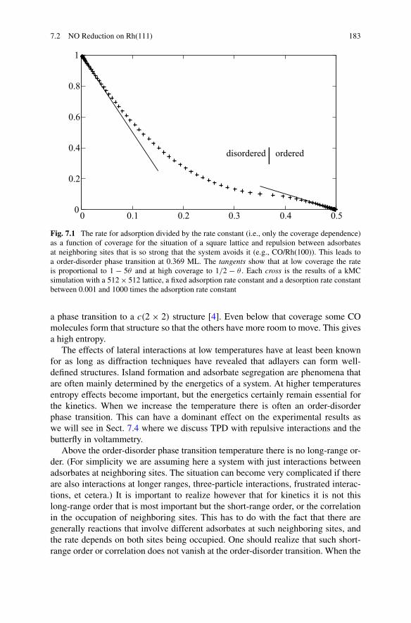
7.2 NO Reduction on Rh(111) 183

Fig. 7.1 The rate for adsorption divided by the rate constant (i.e., only the coverage dependence)as a function of coverage for the situation of a square lattice and repulsion between adsorbatesat neighboring sites that is so strong that the system avoids it (e.g., CO/Rh(100)). This leads toa order-disorder phase transition at 0.369 ML. The tangents show that at low coverage the rateis proportional to 1 − 5θ and at high coverage to 1/2 − θ . Each cross is the results of a kMCsimulation with a 512 × 512 lattice, a fixed adsorption rate constant and a desorption rate constantbetween 0.001 and 1000 times the adsorption rate constant

a phase transition to a c(2 × 2) structure [4]. Even below that coverage some COmolecules form that structure so that the others have more room to move. This givesa high entropy.

The effects of lateral interactions at low temperatures have at least been knownfor as long as diffraction techniques have revealed that adlayers can form well-defined structures. Island formation and adsorbate segregation are phenomena thatare often mainly determined by the energetics of a system. At higher temperaturesentropy effects become important, but the energetics certainly remain essential forthe kinetics. When we increase the temperature there is often an order-disorderphase transition. This can have a dominant effect on the experimental results aswe will see in Sect. 7.4 where we discuss TPD with repulsive interactions and thebutterfly in voltammetry.

Above the order-disorder phase transition temperature there is no long-range or-der. (For simplicity we are assuming here a system with just interactions betweenadsorbates at neighboring sites. The situation can become very complicated if thereare also interactions at longer ranges, three-particle interactions, frustrated interac-tions, et cetera.) It is important to realize however that for kinetics it is not thislong-range order that is most important but the short-range order, or the correlationin the occupation of neighboring sites. This has to do with the fact that there aregenerally reactions that involve different adsorbates at such neighboring sites, andthe rate depends on both sites being occupied. One should realize that such short-range order or correlation does not vanish at the order-disorder transition. When the

184 7 Examples

temperature increases the short-range order decreases, but only gradually convergesto zero. This is the reason why rate equations are also not correct for catalysis athigh temperatures.

And even if the temperature is so high that also the short-range order is negli-gible, the lateral interactions still can not be treated in the form of an effective rateconstant. To see this we need a short derivation of the type we did in Sect. 4.6.Suppose we have an adsorbate A that desorbs and that has interactions with adsor-bates with neighboring sites. Suppose for simplicity that the adsorption sites form asquare lattice. The phenomenological equation (4.73) then says that the probability〈A〉 that a site is occupied changes according to the following equation.

−d〈A〉dt

= W(0)des

⟨ ∗∗ A ∗

∗

⟩+ 4W

(1)des

⟨ ∗A A ∗

∗

⟩

+ 4W(2,1)des

⟨ AA A ∗

∗

⟩+ 2W

(2,2)des

⟨ ∗A A A

∗

⟩

+ 4W(3)des

⟨ AA A A

∗

⟩+ W

(4)des

⟨ AA A A

A

⟩. (7.3)

The probabilities on the right-hand-side specify a particular occupation of a centralsite and its four neighbors. There are different rate constants for these occupations.The coefficients before the rate constants indicate the number of symmetry-relatedways the sites can be occupied.

If we assume that the adsorbates are randomly distributed over the sites, then wecan simplify this expression to

−dθA

dt= W

(0)desθA(1 − θA)4 + 4W

(1)desθ

2A(1 − θA)3

+ [4W(2,1)des + 2W

(2,2)des

]θ3

A(1 − θA)2

+ 4W(3)desθ

4A(1 − θA) + W

(4)desθ

5A, (7.4)

where we have used 〈A〉 = θA and⟨ X2

X1 X0 X3X4

⟩= 〈X0〉〈X1〉〈X2〉〈X3〉〈X4〉 = θX0θX1θX2θX3θX4 . (7.5)

This is as far as we can go without making any assumption besides the one aboutthe random distribution of the adsorbates. To get a further simplification we needto make assumptions about the rate constants. If we assume that they are all equal,then the equation reduces to

−dθA

dt= W

(0)desθA

[θA + (1 − θA)

]4 = W(0)desθA, (7.6)

but this assumption means that there are no lateral interactions.

7.2 NO Reduction on Rh(111) 185

For pair interactions we have

W(n,...)des = W

(0)dese

nϕ/kBT (7.7)

with ϕ the interaction parameter. This simplifies the expression to

−dθA

dt= W

(0)desθA

[θAeϕ/kBT + (1 − θA)

]4. (7.8)

We see that we retain a strongly non-linear dependence of the rate on the coverage.The system NO/Rh(111) that we will discuss here shows most of the effects causedby lateral interactions that we have mentioned above.1 In addition it shows howlateral interactions can change the preferred adsorption site. NO on Rh(111) prefershollow sites, but at high coverages part of the NO moves to top sites. The adsorptionenergy of the top site is much lower than that of the hollow sites, but by moving totop sites a strong repulsion between the adsorbates is avoided.

At temperatures below 275 K NO adsorbs molecularly [5, 6]. It prefers the three-fold hcp site slightly over the threefold fcc site. The difference of the adsorptionenergy depends on the coverage, but it is only in the range of 3 to 8 kJ/mol [7–9].The bridge site and certainly the top site have much smaller adsorption energies.The difference is between 20 to 24 and 61 to 64 kJ/mol, respectively.

NO starts dissociating above 275 K and forms nitrogen and oxygen atoms. Ni-trogen prefers the threefold hcp site just as NO, but oxygen prefers the threefoldfcc site. The difference with the other threefold site is again small: between 9 and14 kJ/mol for nitrogen, and between 6 and 10 kJ/mol for oxygen. At low coverageall of the NO dissociates, but as the coverage increases less and less NO dissociatesand the temperature at which dissociation starts increases.

An explanation why less NO dissociates at higher coverages is that there are sim-ply no sites available. If the system is modeled with one (threefold) site per unit cell[9, 10], then the suppression of the NO dissociation can simply be explained becauseat high coverage there are not enough sites available for the atoms that are formedwhen NO dissociates. NO occupies only one site, but the atoms after dissociationoccupy two. When all NO dissociates the number of occupied sites doubles. Whenthe initial coverage of NO is higher than 0.5 ML, all sites are occupied before allNO has dissociated.

The 1-site model above has three shortcomings. First, it does not show that thedissociation of NO becomes already suppressed below 0.5 ML, and the maximumcoverage of NO is only 0.75 ML. Second, it does not explain the temperature de-pendence. In fact, it does not have any temperature dependence related to the initialcoverage of NO. Third, DFT results indicate that at least the other threefold sitesshould also play a role [7–9]. In fact, LEED shows that the NO adlayer with a cov-

1Parts of Sect. 7.2 have been reprinted with permission from C.G.M. Hermse, F. Frechard, A.P. vanBavel, J.J. Lukkien, J.W. Niemantsverdriet, R.A. van Santen, A.P.J. Jansen, Combining density-functional calculations with kinetic models: NO/Rh(111), J. Chem. Phys. 118, 7081 (2003). Copy-right 2003, American Institute of Physics.

186 7 Examples

erage of 0.75 ML has on equal distribution of the NO molecules over both threefoldsits and the top site [11, 12].

It is clear from this that lateral interactions play an important role in the system.So the 1-site model should be extended with lateral interactions. This can reproducethe dissociation behavior as far as initial coverage and temperature dependence isconcerned, but not the maximum NO coverage. Moreover, the lateral interactionsthat are needed for the 1-site model to reproduce the experimental Temperature-Programmed Reaction (TPR) spectra are an order of magnitude lower than thoseobtained from DFT calculations [7–9].

A correct model is obtained by including lateral interactions and the two three-fold and the top sites. NO can occupy all three sites, but is has a clear preference forthe threefold sites. The atoms are only allowed to occupy threefold sites. DFT cal-culations give lateral interactions for sites at a distance of 1

3

√3dRh−Rh, dRh−Rh, and

23

√3dRh−Rh with dRh−Rh the distance between neighboring substrate atoms. At the

shortest distance of 13

√3dRh−Rh the interactions are so strongly repulsive that they

can be modeled as site blocking. At a distance of dRh−Rh there is still a strong re-pulsion of at least 24 kJ/mol. This repulsion is still so strong that the system avoidsit, and it does not show up in the results of kinetic experiments. It does howeverstrongly determine the structure of the adlayer (it can be regarded as site blockingfor the structures as well), and only when the structure of the adlayer changes theadsorbates occasionally get as close as a distance dRh−Rh of each other. To avoidthis repulsion at coverages above 0.5 ML NO moves to top sites. There is also suchstrong repulsion at 2

3

√3dRh−Rh between atoms, between atoms and NO, and be-

tween NO molecules.The system and the model of it shows many of the phenomena that result from

lateral interactions that were discussed before. At low temperatures NO forms vari-ous superstructures depending on coverage. At 0.5 ML a c(4 × 2)-2NO structure isformed and at 0.75 ML a (2 × 2)-3NO structure (see Fig. 7.2) [11–13]. The maxi-mum coverage of 0.75 ML is a consequence of the fact that it is the maximum cov-erage that has no NO molecules at distance dRh−Rh. The phase transitions betweenthe structures are here not caused by temperature, but by a change in coverage. Theordered structures also show an order-disorder phase transition in the kMC simula-tions when the temperature increased and if we leave out the NO dissociation.

When NO starts dissociating we get an adlayer with NO, N, and O atoms thatsegregate (see Fig. 7.3). There is little difference in N–N, O–O, and N–O interac-tions. This means that the nitrogen and oxygen atoms mix. The interactions withNO are however different. In particular, the repulsion between NO and the atoms islarger than the average between the atom-atom and the NO–NO interactions, mainlybecause the NO–NO repulsion is much weaker. As a consequence we have the seg-regation as in the figure. There is a strong similarity with island formation, becausethe interactions are formally equivalent to one with attractive interactions betweenthe atoms and between the NO molecules.

That lateral interactions affect the kinetics is clear, but the effects are not soclear-cut as those for the structures. The suppression of the NO dissociation when

7.2 NO Reduction on Rh(111) 187

Fig. 7.2 Ordered structures of NO/Rh(111). The coverage on the left is 0.5 ML and on the right0.75 ML. Large circles depict NO molecules, small circles vacant sites. Top sites are gray andhollow sites are black. The structure of 0.5 ML has zigzag chains of molecules at alternating fccand hcp sites with a vacant top site in between. The structure of 0.75 ML has a honeycomb structureof molecules at hollow sites with molecules at top sites in the centers of the hexagons [9]

the initial coverage increases is clearly due to the increase in repulsive lateral inter-actions. This effect becomes even noticeable at quite low coverage (see Fig. 7.4).The same thing explains the higher temperature at which the dissociation starts. Athigh initial coverage the dissociation is partial or even suppressed completely. In thespectra there is a second peak for dissociation at high temperature. This results fromdesorption of NO that frees sites and makes new dissociation reactions possible.

One consequence of the lateral interactions that is easier to explain is the tem-perature at which NO desorbs that does not dissociate. The adsorption energy ofisolated NO has a value that suggests a much higher desorption temperature. Fortop sites there is a repulsion of six neighboring NO molecules at hollow sites. Thisis always the same, so the desorption from top sites is always at the same temper-ature but at a lower temperature than might be inferred from the adsorption energyfor an isolated NO molecule. The desorbing NO from hollow sites that is observedin TPR spectra is surrounded by nitrogen and oxygen atoms. These NO moleculesfeel a strong repulsion from these atoms, and also desorb at a lower temperature.

188 7 Examples

Fig. 7.3 Snapshot of part ofthe adlayer during asimulated TPR experiment ofNO/Rh(111). The initialcoverage of NO was 0.75 ML(see Fig. 7.2). The initialtemperature was 250 K andthe heating rate was 10 K/s.The snapshot was taken at490 K. Black circles depictoxygen atoms, gray circlesnitrogen atoms, and whitecircles NO molecules. Thesimulated system consisted of264 × 264 sites forming asimple hexagonal lattice.A third of the sites was fcc, athird hcp, and a third top.Labels were used todistinguish the type of site [9]

There are two peaks for N2 desorption. There is a narrow peak at a relatively lowtemperature and a broad peak at high temperature. The narrow peak is associatedwith the desorption of NO that makes new dissociation reactions possible. This cre-ates nitrogen atoms in the adlayer with a very high coverage and a fraction of them

Fig. 7.4 Temperature-Programmed Reaction spectra (rates in arbitrary units versus temperaturein Kelvin) of NO/Rh(111). The heating rate is 10 K/s. There are no spectra for oxygen desorptionbecause this takes place at higher temperatures and has not been included in the simulations. Thenumbers next to the curves are the initial coverages of NO. The spectra have been obtained byaveraging over 100 kMC simulations with a simple hexagonal 264 × 264 lattice representing thetop, fcc, and hcp sites [9]

7.3 NH3 Induced Reconstruction of (111) Steps on Pt(111) 189

is pushed of the surface. The broad peak is formed after all NO molecules have ei-ther dissociated or desorbed. It results from nitrogen surrounded by oxygen atoms.

7.3 NH3 Induced Reconstruction of (111) Steps on Pt(111)

Another reason why macroscopic rate equations may fail is that the substrate isnever homogeneous. We may have a bimetallic catalyst, but more common is that thesurface has defects. As a consequence different parts of the surface have sites withdifferent adsorption energies and reactivities. Using a model with a single coverageis then bound to fail, but even if we use different coverages for the different parts ofthe substrate we make an approximation that may not be justifiable.

Suppose that we have a simple adsorption-desorption equilibrium on a squarelattice, but that there is a step. Suppose for simplicity that we can model this with asingle row of sites that have a desorption rate constant that differs from that of othersites. The macroscopic rate equations are then

dθn

dt= kads(1 − θn) − k

(terrace)des θn + D

a2[θn+1 + θn−1 − 2θn] (7.9)

for n = 0 and

dθ0

dt= kads(1 − θ0) − k

(step)

des θ0 + D

a2[θ1 + θ−1 − 2θ0]. (7.10)

Here θn is the probability that a site a distance |n|a from the step is occupied. Siteswith n > 0 are on one side of the step and those with n < 0 on the other. Theparameter a is the distance between the sites, kads is the adsorption rate constantkdes is the desorption rate constant, and D/a2 the hopping rate constant (D is thediffusion coefficient). The derivation of these rate constants is very similar to theones in Sect. 4.6.

If the adsorbates do not hop to neighboring sites (D = 0), then we find

θ0 = kads

kads + k(step)

des

and θn = kads

kads + k(terrace)des

(7.11)

for n = 0. In this case using two coverages, one for the step and one for the terraces,is justified. If the adsorbates are allowed to hop (D = 0), then this is no longer thecase. We will see that we get a gradient in the coverage away from the step.

The general solution of the rate equations can be written as

θn = kads

kads + k(terrace)des

+ Bλ−|n|. (7.12)

Substitution of this expression in the rate equations for the terrace sites yields

λ + 1

λ= 2D/a2 + kads + k

(terrace)des

D/a2(7.13)

190 7 Examples

Fig. 7.5 Snapshot of part of a Pt-Ru electrode during a simulation of a linear sweep voltammetryexperiment in which CO is replaced by OH. The Ru part of the electrode is completely coveredby CO (gray circles) or OH (white circles). The Pt part is partially covered by CO (black circles)but a lot of it is vacant. The formation of OH on the electrode takes place initially on the Ru sideof the Pt-Ru interface. That OH reacts with CO on the Pt side of the interface which leads to thevacancies on Pt. The vacancies on Ru are filled by new OH being formed [14]

for the parameter λ. There are two solutions, but only the one with λ > 1 is physi-cally acceptable, because the second term of the right-hand-side of equations (7.12)should go to zero for large |n|. The appropriate value for λ is given by

λ = 1

2

[μ +

√μ2 − 4

](7.14)

with μ equal to the right-hand-side of Eq. (7.13). Substitution of expression (7.12)in the rate equation for the step gives a linear equation for B . The solution of it is

B = kads(k(step)

des + k(terrace)des )

[k(step)

des − kads + 2D(λ − 1)/a2][kads + k(terrace)des ]

. (7.15)

The important point however is that, although all terrace sites have the same prop-erties, their coverage is not the same because of the presence of the step.

Another example is shown in Fig. 7.5. It shows a snapshot of a model of a Pt-Ru electrode during a voltammetry experiment [14]. Initially the whole electrodeis covered by CO except for a few vacancies. The initial potential is low and noreactions take place. The potential is then increased which causes water to adsorbdissociatively forming OH on the electrode. The OH reacts with CO to form CO2and a proton, which both desorb immediately. These reactions take place first at the

7.3 NH3 Induced Reconstruction of (111) Steps on Pt(111) 191

Pt-Ru interface. The OH forms on Ru and the CO is taken from Pt. The resultingvacancy on Ru is rapidly filled by another OH, but on Pt we get a gradient of COmolecules diffusing to the Pt-Ru interface.

When we cut a crystal we get a surface that is not necessarily stable. That surfacewill then change its structure. Such a change is called a reconstruction. This oftenleads to another form of heterogeneity of the substrate than the ones mentionedabove. The structure of surfaces is also often changed by catalytic reactions [15,16]. An example is discussed in Sect. 7.5. As a simpler model system for sucha restructuring process we consider here a stepped metal surface and look at thereconstruction of a step. Due to their reduced coordination number atoms at stepsoften exhibit an enhanced catalytic activity [17]. We discuss here the restructuringof a stepped Pt(111) surface in the presence of adsorbed ammonia. We look at asingle step and on the details of the meandering of such step [18].2

A Pt(443) surface in its clean state consists of monatomic (111) steps separatedby seven lattice units wide (111) terrace (Fig. 7.6a and b). When this surface is ex-posed to ammonia at 300 K with pNH3 = 10−6 mbar first individual Pt atoms movealong the step edge as shown by Figs. 7.6c and d. These atoms migrate and becomeagain attached rigidly to the step edge. Thus holes and protrusions are formed alongthe step edges generating a meandering of the step edges as shown in Fig. 7.6e.This meandering takes place in about 10–15 minutes. The dynamics of the substratechanges are frozen in when after approximately 30 minutes an ordered (2 × 2) am-monia overlayer forms on the (111) terraces visible in the STM image in Fig. 7.6f.

Several aspects of the energetics of meandering are obvious. The number of Pt-Ptbonds of the step atoms decreases when the step starts to meander thus increasingthe step energy of the step. Simultaneously, due to bond-order conservation the re-maining bonds of the Pt step atoms will become stronger, and the NH3 adsorptionenergy is expected to be highest on Pt step and kink atoms [19]. A first guess wouldtherefore be that the meandering is driven by the gain in ammonia adsorption energycaused by creation of low coordinated sites. To check this explanation plane-waveDFT calculations were performed of steps with various structures with and with-out ammonia [20]. Ammonia adsorbs on top sites of the Pt surface. The adsorptionenergy at a kink site is 17 kJ/mol larger than at a straight (111) step, but it costs41 kJ/mol to form the kink.

Ammonia adsorption on a surface with a single step was modeled allowing Ptatoms and ammonia molecules to diffuse on the upper and lower terrace but notacross the step [18]. To account for the formation a (2 × 2)-structure of ammonia ata 1/4 ML coverage molecules were not allowed to become nearest- or next-nearestneighbors. Adsorption of ammonia was assumed to be a simple direct adsorption.

kMC simulations without ammonia do not show any meandering at 300 K. Thisis not surprising as the energy changes are much higher than the thermal energy.

2Parts of Sect. 7.3 have been reprinted with permission from X.Q. Zhang, W.K. Offermans, R.A.van Santen, A.P.J. Jansen, A. Scheibe, U. Lins, R. Imbihl, Frozen thermal fluctuations in adsorbate-induced step restructuring, Phys. Rev. B 82, 113401 (2010). Copyright 2010, American PhysicalSociety.

192 7 Examples

Fig. 7.6 STM images showing the meandering of the step edges on a Pt(443) surface duringexposure to ammonia at 300 K with pNH3 = 10−6 mbar. t = 0 refers to at the beginning of adsorp-tion when the coverage is zero. (a) Structural model of Pt(443); (b) clean surface; (c) t = 3 min.;(d) t = 15 min.; (e) t = 15 min. The image in (f) at t = 35 min. at maximum coverage displays for-mations of a 2 × 2-NH3 structure. Sizes of the imaged areas are (b)–(d) 50 Å × 30 Å, (e) 150 Å ×95 Å, and (f) 45 Å × 30 Å [18]. (Color figure online)

Only when the temperature is increased to around 600 K or higher there are devi-ations from the straight (111) step. Starting with a bare surface it is observed thatduring ammonia adsorption the initially straight (111) step starts meandering as thecoverage of ammonia builds up. This is because part of the energy costs to formkinks is offset by the higher adsorption energy of ammonia at kink atoms. As aconsequence there is a decrease of the stiffness of the step.

As long as there are kinks and lone Pt atoms without ammonia the shape of thestep keeps changing. The meandering stops however almost completely when nomore ammonia can be added to the step edge. At that point some Pt atoms at the

7.4 Phase Transitions and Symmetry Breaking 193

Fig. 7.7 Snapshot of a kMC simulation showing part of a step formed with NH3. Open circlesare Pt atoms without NH3, closed circles are Pt atoms with NH3. The lower terrace is in a lightershade [18]

step edge can still move, but each Pt hop is immediately followed by its reversehop. The shape of the step is then fixed. More extensive changes to the step do notoccur because they would now drive ammonia to less favorable adsorption sites, andwould involve structures with energies that are substantially higher than the thermalenergy. If the coverage of ammonia is increased further, then also the remaining Pthops at the step edge become suppressed. This is because the Pt atoms at the stepbecome blocked by ammonia at the lower terrace. It takes about 20 minutes to freezethe step, which is in good agreement with the experimental results. Also the shapeof the final step is in good agreement with the STM images (see Fig. 7.7).

So the behavior of the step based on the STM experiments and the kMC simula-tions can be summarized as follows. Without ammonia the straight (111) step is en-ergetically the most favorable structure, and hence the equilibrium structure. Thereare no fluctuations in the structure at T = 300 K, because structural deviations froma straight edge have energies that are substantially higher than the thermal energy.Adding ammonia still leaves the structural deviations energetically unfavorable, butthe energy difference is now reduced strongly enough to allow for thermal fluctu-ations. This leads to meandering. When the density of ammonia at the step edgebecomes high, the diffusion of Pt atoms is suppressed because any jump generateslocally energetically unfavorable configurations, because ammonia would be forcedto unfavorable sites. The final structure of the step can therefore be regarded as afrozen thermal fluctuation.

7.4 Phase Transitions and Symmetry Breaking

Phase transitions are notoriously difficult to predict accurately. The Ising model ona square lattice is a prototype model to study phase transitions. It shows an order-disorder phase transition that can be solved analytically [4]. The exact temperatureof the phase transition is a factor 2 ln(1 + √

2) ≈ 1.763 lower than the temperaturethat is obtained from a Mean-Field Approximation similar to the one on which themacroscopic rate constants of chemical kinetics are based. Such a large discrepancyis typical, and forms a good reason for doing simulations.

194 7 Examples

The Ising model shows an example of an equilibrium phase transition that iscaused by the interactions between spins. Such phase transition can also be ob-served in adlayers, although there it originates from the interactions between adsor-bates. In fact, adlayers can show quite complicated phase diagrams as a function oftemperature, coverages, and possibly composition, because of multiple interactionsof various strengths between the adsorbates and different adsorption sites that mayplay a role. Equilibrium phase transitions may show up in kinetic experiments: inparticular, experiments in which reaction conditions are changed. The conditions atwhich the transition occurs will then also depend on the rate with which the changeof the conditions takes place.

There are also other phase transitions possible that are typical for systems withirreversible reactions. They originate from the fact that for some reaction conditionsthere may be more than one stable steady state, and changing reaction conditionsmay make the one that a system is unstable. This results then in non-equilibrium orkinetic phase transitions. When macroscopic rate equations are used they are alsocalled bifurcations [21, 22]. In fact, much more complicated situations may ariseshowing oscillations, pattern formation, and chaotic behavior [23, 24].

In this section we show two examples of equilibrium phase transitions showingup in kinetic experiments. In one lateral interactions cause a phase transition, inthe other the configurational entropy is responsible. We also show an example withkinetic phase transitions. All examples are kept simple so as to illustrate the phasetransitions most clearly.

7.4.1 TPD with Strong Repulsive Interactions

One of the clearest examples of the advantage of kMC simulations over macroscopicrate equations is formed by simple desorption with strong lateral interactions. Ifwe take for example a square lattice, an initial situation with all sites occupied,and repulsive interactions between nearest neighbors, then the following happens.Initially, each adsorbate has the same tendency to desorb. However, if one adsorbatedesorbs then its former neighbors suddenly feel less repulsion and become adsorbedmore strongly. This means that desorption takes place in two stages. First about halfthe adsorbates desorb, because they have many neighbors. After these adsorbateshave desorbed the structure of the adlayer is that of a checkerboard, with almost alladsorbates having no neighbors. Because these adsorbates feel little or no repulsionfrom other adsorbates they desorb at a later stages.

So we have a phase transition at half a monolayer coverage. At higher cover-ages the adlayer consists of patches with a checkerboard and patches with a 1 × 1structure (θ = 1). At lower coverages the adlayer consists again of patches with acheckerboard but with vacant areas in between. Also note that there is a symmetrybreaking. Initially all sites are equivalent, but after half the adsorbates have des-orbed alternate sites are occupied and vacant. Ordinary macroscopic rate equationsare not able to describe this symmetry breaking, because they assume that all sites

7.4 Phase Transitions and Symmetry Breaking 195

Fig. 7.8 Domain formation during desorption with strong repulsive interactions. This is a snapshotfrom a simulation of a Temperature-Programmed Desorption experiment with adsorbates with arepulsion of 6.65 kJ/mol (see Fig. 7.9). The coverage is 0.29 ML. All adsorbates are equivalent butblack and gray adsorbates are from different domains

are equivalent during the whole process. We can split the macroscopic rate equationsin two: one for the sites with the adsorbates that desorb first, and one for the siteswith adsorbates that desorb later. However, the equations for both sites are equiva-lent and the symmetry breaking only occurs if the initial state already has a smalldifference in the occupations between the sites with the early desorbers and the siteswith the late desorbers. For kMC simulations such an unrealistic initial conditionis not necessary. In kMC fluctuations in the times when reactions occur cause thesymmetry breaking as they do in real systems. Such fluctuations are not included inmacroscopic rate equations.

The fluctuations determine which adsorbates desorb first, and also affect thestructure of the adlayer when the coverage has been more of less halved. A per-fect checkerboard structure is only found when the adsorbates also diffuse fast andwhen the temperature is well below the order-disorder phase transition temperature.For small system sizes the diffusion need not be so fast as for large system sizes.Diffusion has to make sure that no domains are formed. Simulations show that evenat relatively small systems with say a 128 × 128 lattice it is almost impossible toavoid domain formation (see Fig. 7.8).

Figure 7.9 shows a TPD spectrum for a system with repulsive interactions. Weshow TPD instead of isothermal desorption, because the latter shows the two stagesin the desorption only in how fast the coverage and the desorption rate decreases.If the coverage is plotted logarithmically, then we get first a straight line with a

196 7 Examples

Fig. 7.9 Temperature-Programmed Desorption spectrum (desorption rate vs. temperature inKelvin) of adsorbates repelling each other. The fat line is the total desorption rate. The thin linesare separate contributions of adsorbates desorbing with a number of nearest neighbors given by thenumber next to the curve. Activation energy for desorption is Eact = 121.3 kJ/mol and the prefac-tor is ν = 1.435 · 1012 s−1. These numbers were taken from CO desorption from Rh(100) at lowcoverage. The repulsion between two adsorbates is 6.65 kJ/mol. The heating rate is 5 K/s and theinitial coverage 1.0 ML

large negative slope, followed by a straight line with a smaller, in absolute sense,negative slope. In TPD the two stages are much clearer, because the desorption ratehas two peaks. The figure shows that the second stage (i.e., the second peak) hasalso contributions from adsorbates with one, two, and even three neighbors, whichis due to the fact that the first stage never forms a perfect checkerboard structure andthe fact that many adsorbates first diffuse to a site with neighbors and desorb fromthat site. If the repulsion becomes very strong, then even more than two peaks canform.

In real systems the effects of lateral interactions are generally not so unambigu-ous. The lateral interactions have to be strong enough so that a well-defined struc-ture is formed when half the adsorbates have desorbed. If this is not the case thenthe lateral interactions only show up by shifting or broadening a single peak whenthe initial coverage is increased. When lateral interactions are strong enough, thenthey may also push adsorbates to other adsorption sites. These sites have a loweradsorption energy, but overall the energy is lowered because it lessens the repul-sion between the adsorbates. The result may even be an adlayer structure that isincommensurate with the substrate. Finally, lateral interactions need not just be be-tween nearest neighbors. Interactions between next- and next-next-nearest neigh-bors are not uncommon. Longer range interactions can sometimes be excluded [25],but charged adsorbates might have long-range interactions, which may explain verybroad desorption peaks [26, 27].

7.4 Phase Transitions and Symmetry Breaking 197

Fig. 7.10 Lateral interactionmodel on a fcc(111) lattice.The adsorbed anion binds totwo surface atoms in abridged fashion (blackatoms), making bonding tothe first shell of neighboringsites (gray) impossible

7.4.2 Voltammetry and the Butterfly

The adsorption of anions on single-crystal electrode surfaces usually gives rise tothe appearance of ordered adsorbate adlayers. The formation of these ordered adlay-ers is often accompanied by a characteristic sharply peaked current response in thecyclic voltammetry, commonly referred to as “butterfly” in the electrochemical com-munity [28–30]. We discuss this butterfly for a model of adsorption of (bi)sulfateon fcc(111) surfaces [31].3 The simulated voltammogram shows a broad peak as-sociated with adsorption in a disordered phase, and a sharp one associated with adisorder-order transition in the adlayer. The disorder-order transition converts theadlayer with a coverage of 0.18 ML into a (

√3 × √

7) ordered structure with a cov-erage of 0.20 ML. The (

√3 × √

7) structure with 0.20 ML saturation coverage isexperimentally known for the adsorption of anions from sulfuric acid solution onmany fcc(111) surfaces. The anion involved is either bisulfate (HSO−

4 ) or sulfate(SO2−

4 ). The reactions are

A2− + ∗∗ � Aads + 2e−, (7.16)

where ∗∗ denotes an vacant bridge site (formed by two vacant surface atoms): each∗ corresponds to a surface atom. Figure 7.10 shows the (111) substrate and theneighboring sites around a bridge-bonded adsorbate. There is a shell of purely hardinteractions, in which the simultaneous bonding of two anions to neighboring sitesis simply excluded. This model is equivalent to the elongated hard hexagon modelconsidered by Orts et al. [32].

Because of the hard interactions the phase transition here is different from theone observed in TPD with finite repulsive interactions (see Sect. 7.4.1). The phasetransition there involves a change in the energetics. This is not the case here. Thesystem avoids the hard interactions, and the energy of the adlayer is always zero. Thestructure of the adlayer is only determined by the configurational entropy. (We are

3Parts of Sect. 7.4.2 have been reprinted with permission from C.G.M. Hermse, A.P. van Bavel,

M.T.M. Koper, J.J. Lukkien, R.A. van Santen, A.P.J. Jansen, Modelling the butterfly: (√

3 × √7)

ordering on fcc(111) surfaces, Surf. Sci. 572, 247 (2004). Copyright 2004, Elsevier.

198 7 Examples

ignoring here the interactions of the adsorbates with the substrate. These interactionsonly determine the coverage. Their contribution is constant for a give coverage, andhence they do not affect the structure of the adlayer.)

In a voltammetry experiment the electrode potential E is varied: here we startwith a low value without adsorbates on the electrode surface, then increase the po-tential and monitor the coverage θ . The rate constants for adsorption and desorptionare

kads = k0 exp

(−αadsγ eE

kBT

)(7.17)

kdes = k0 exp

(αdesγ eE

kBT

)(7.18)

where αads = 1/2 is the transfer coefficient for adsorption, γ is the electrosorp-tion valency (taken −2), and e is the elementary charge. The exponent describesthe potential-dependent adsorption of the anion. The definitions in Eqs. (7.17)and (7.18) imply that in our model at zero potential the adsorption rate constantis equal to the desorption rate constant: kads = kdes = k0. The transfer coefficientsare related as follows.

αdes = 1 − αads. (7.19)

The diffusion steps were defined as hopping between neighboring bridge sites.Apart from the dependence of θ on E, we are particularly interested in the com-

pressibility dθ/dE of the adlayer, as this quantity is proportional to the Faradaiccurrent measured in an electrochemical voltammetry experiment

j = −eγΓmνdθ

dE, (7.20)

where j is the Faradaic current in A/cm2, Γm is the number of surface sites per unitsurface area (taken to be 1.5 × 1015 sites/cm2), and ν is the sweep rate (typically50 mV/s).

Figure 7.11 shows the voltammogram obtained from kMC simulations. Thedisorder-order transition at 0.11 V is particularly sensitive to the level of equili-bration: an insensitivity of this peak to reducing the sweep rate indicates that thesurface is well equilibrated. The simulations were therefore done by choosing therates of adsorption, desorption and diffusion such that upon reducing the sweep ratefrom 50 to 5 mV/s the disorder-order transition peak is shifted by less than 5 mV.This is also what is expected experimentally. The values fulfilling this requirementare k0 = 103 s−1 and k0

diff = 105 s−1. The sweep rate used was 50 mV/s.Going from more negative to more positive potential, the anion adsorbs between

−0.1 and 0.1 V in a disordered phase (see snapshots in Fig. 7.12a, b). This results ina broad adsorption peak in the voltammogram. There is a disorder-order transition at0.11 V, indicated by the sharp peak in the voltammogram. At this voltage the anioncoverage rapidly increases from 0.18 to 0.20 ML, which is the saturation coverage.This result was previously obtained by Orts et al. using an elongated hard hexagontype model [32]. The onset of the disorder-order transition is shown in Fig. 7.12c.

7.4 Phase Transitions and Symmetry Breaking 199

Fig. 7.11 Voltammograms (current in arbitrary units versus electrode potential in V) averagedover 500 kMC simulations with a hexagonal 128 × 128 lattice, temperature T = 300 K, and sweeprate of 50 mV/s. The width of the terraces in the surface with the steps is 16 rows

(√

3 × √7) Islands are forming, and, as indicated in the figure, these can have three

different orientations. After the disorder-order transition (at potentials of 0.12 V andabove) only large (

√3 × √

7) domains are present on the surface. These typicallyconsist of more than one thousand adsorbates. At 0.10 V, the surface is occupied byanions which have three different orientations. Packing of equal amounts of theseanions of different orientations is only possible up to about 0.18 ML. This causes adecrease in the adsorption current close to 0.10 V. It is only with the alignment ofthe adsorbates in the same direction that more anions can adsorb, since the ordered(√

3 × √7) structure allows for a tighter packing of anions.

The presence of defects in the surface prevents long-range ordering of adsor-bates. The voltammogram is therefore expected to change when steps are intro-duced. We have investigated this effect by introducing step sites at regular intervalsin our model. Bonding to these step sites is excluded, and the adsorbates are alsonot allowed to diffuse across the steps. Our results indicate that for different terracesizes only the disorder-order transition peak changes: the broad peak associatedwith adsorption in a disordered phase hardly changes. The disorder-order transitionpeak decreases in intensity with decreasing terrace size (Fig. 7.11). The saturationcoverage decreases as well. For terrace sizes of 64 and larger, the orientation ofthe (

√3 × √

7) domains is independent of the step orientation: i.e., islands of allthe three different orientations of the (

√3 × √

7) structure are found. The intensityof the disorder-order transition peak is comparable to the one for the case withoutsteps. For terrace sizes of 16 and 32, the (

√3 × √

7) domains align to the steps, asshown in Fig. 7.13. For an even smaller terrace size of 8, no ordering is observed,even if the sweep rate is reduced to 5 mV/s.

200 7 Examples

Fig. 7.12 Snapshots of the surface during anion adsorption. Before the disorder-order transition(panel (a) and (b)) there is no ordering; during the disorder-order transition (

√3 × √

7) islandsgrow ((c); the three different domain orientations are indicated by the small arrows); after thedisorder-order transition large islands dominate (d). The (

√3 × √

7) unit cell is indicated in (d)

7.4.3 The Ziff–Gulari–Barshad Model

Although the work by Ziff, Gulari, and Barshad does not represent the first appli-cation of Monte Carlo to model surface reactions it is probably the most influentialwork of its type [33]. There are several reasons for that. It deals with CO oxidationwhich was and still is a very important process in catalysis and surface science. It isa very simple model, which makes it generic. Its simplicity also makes it possibleto analyze in detail the relation between the microscopic reactions and the macro-scopic properties. It has shown the shortcomings of the macroscopic rate equationsand what the origin of these shortcomings were. It has shown that kMC simula-tions can describe kinetic or non-equilibrium phase transitions. In fact, apart fromthe first-order phase transition also known from macroscopic rate equations, it hasshown that there is a continuous phase transition as well.

We present here the model, which we will call the Ziff–Gulari–Barshad (ZGB)model, in its generic form. There are two adsorbates: A and B. If one wants to use

7.4 Phase Transitions and Symmetry Breaking 201

Fig. 7.13 Snapshot of the surface at 0.25 V after anion adsorption for the model with first neighborshell exclusion and a terrace width of 16. Bonding to the steps (shaded circles) is forbidden. Thearrows show the alignment of the adsorbate islands (in black) to the steps (shaded), the coverageequals 0.19 ML

the ZGB-model for CO oxidation, then A stands for CO and B for atomic oxygen.There are three reactions in the model. Adsorbate A can adsorb at single vacantsites. Adsorbate B can adsorb, but as it forms diatomic molecules in the gas phase,two neighboring vacant sites are needed. An A will react with a B if they are nearestneighbors. This reactions is infinitely fast, so this takes place immediately after anadsorption. We can write the reaction as

A(gas) + ∗ → A(ads)

B2(gas) + 2∗ → 2B(ads) (7.21)

A(ads) + B(ads) → AB(gas) + 2∗where ∗ is a vacant site, “ads” stands for an adsorbed species, and “gas” for a speciesin the gas phase. The reactions involving two sites can only take place on neighbor-ing sites. Focusing on the sites only we have

∗ → A

2∗ → 2B (7.22)

A + B → 2∗The adsorbates do not diffuse in the original model, and the lattice is a square one.There are many extensions to this model dealing, among others, with desorption ofCO and oxygen [34], diffusion of the adsorbates [34], an Eley–Rideal mechanismfor the oxidation step, physisorption of the reactants, lateral interactions between the

202 7 Examples

adsorbates [34], blocking of the sites due to poisoning with lead or alloying [35, 36],reconstruction of the surface (see Sect. 7.5.2) [37–44], and an inert adsorbate thatcauses oscillations [45, 46].

The rate constant for adsorption of A can be derived as in Sect. 4.6.3, and foradsorption of B as in Sect. 4.6.7. The results are

WA,ads = yPAsiteσA√2πmkBT

(7.23)

WB,ads = 2(1 − y)PAsiteσB

4√

2πmkBT. (7.24)

The σ ’s are sticking coefficients. The quantity y is the fraction of the molecules inthe gas phase that are A’s. If we assume that the sticking coefficients are equal toeach other, then we can simplify the rate constants to y and (1 − y)/2, respectively,by replacing time t by τ = tPAsiteσA/

√2πmkBT . We see that then the model de-

pends only on one parameter: i.e., only on y.Simulations show that there are three states for the system. One possibility is that

the surface is completely covered by A’s. There are no reactions that can take thesystem out of this state. Such a state is called on absorbing state (see Sect. 2.2.1). Incatalysis one talks in such a case of A poisoning, because it leads to the undesirablesituation that the reactivity is zero. There is another absorbing state, but then withB poisoning. If the parameter y is below a critical value y1, then the system willalways evolve into the B poisoning state. If the parameter y is above another criticalvalue y2, then the system will always evolve into the A poisoning state. For y < y1there are so many B2 molecules in the gas phase that B adsorption will outcompetethe A’s for the vacant sites that are formed by the reaction between the A’s and B’s.To same thing happens for y > y2 except in this situations the A adsorption wins.At y1 and at y2 there is a kinetic or non-equilibrium phase transition.

For y1 < y < y2 there is a third state with A’s and B’s on the surface and a non-zero reactivity. Figure 7.14 shows how the reactivity and the coverage dependenceon y. Note that all quantities change discontinuously at y2. The phase transition atthat value of y is therefore called a first-order transition. At y1 the quantities changecontinuously, so we have a continuous (or second-order) phase transition. Macro-scopic rate equations also predict the first-order phase transition, but not the contin-uous one. Moreover, the first-order phase transition is predicted by the macroscopicrate equations to be at y1 = 2/3, whereas the best estimates from kMC simulationsare y2 = 0.52560 ± 0.00001 [47, 48]. The continuous phase transition is estimatedto be at y1 = 0.39065 ± 0.00010 [49].

Figure 7.15 shows the reason for the discrepancy between the kMC results andthose of macroscopic rate equations. The adlayer is definitely not a random mixtureof adsorbates. The reason is the fast reaction between the A’s and B’s. This reactioncauses segregation of the adsorbates. Isolated A’s will not last long on the surface,because a B may adsorb on one of the vacant neighboring sites that will immediatelyreact with the A which will remove the A from the surface. For a similar reasonisolated B’s will be rare. Only islands of the same kind of adsorbate can last, becausethe particles in the center of an island have no neighboring sites onto which other

7.5 Non-linear Kinetics 203

Fig. 7.14 Phase diagram ofthe Ziff–Gulari–Barshadmodel. The coverages and theAB formation per unit timeper site are shown as afunction of the y parameter

particles can adsorb with which they will react. These islands are formed randomly.Islands of B are larger. They need be because A’s need only one vacant site foradsorption and can relatively easily break them up. Islands of A can be smaller, B’sneed two neighboring vacant sites for adsorption and have more difficulty to removeA’s.

7.5 Non-linear Kinetics

The ZGB-model of Sect. 7.4.3 has shown that also the reactions themselves canresult in a structured adlayer. There have been some claims that this was becausethere was no diffusion in the ZGB-model but, as the A + B model has shown, alsowith diffusion the adlayer is not necessarily homogeneous.

Here we will look at other systems for which reactions and other processes canlead to interesting structured adlayers but also to oscillations and other forms ofnon-linear kinetics. These systems showing non-linear kinetics have mainly beenstudied with rate equations or with reaction-diffusion equations [23, 24, 50]. Suchsystems are difficult for kMC simulations. If one does a kMC simulation with a

Fig. 7.15 Snapshots of the adlayer in the Ziff–Gulari–Barshad model for y = 0.5255 a value justbelow the first-order transition point. The black islands are formed by B’s. The A’s form the whiteislands. Vacant sites are gray

204 7 Examples

small system size then fluctuations can be present that can easily be mistaken foroscillations. Even if the oscillations are real, their amplitude often decreases whenthe system size is increased. This is because local oscillations at different parts ona substrate may be out-of-phase. The variations in the local reactivities will thenaverage out and there will not be a global oscillation. There needs to be a so-calledsynchronization mechanism that couples the local oscillations. It is much easierto get global oscillations with rate equations, because they assume a priori that thecoverages are the same everywhere. It is a bit harder to get oscillations with reaction-diffusion equations [50]. They do allow variations in the coverages as a function ofposition, but they ignore fluctuations that tend to dephase local oscillations. Suchfluctuations are of course present in kMC simulations, which means that they formthe hardest test to see if oscillations can really exist in a given system.

Non-linear kinetics is generally only found in systems that are quite complicated.The best studied system is probably that of CO oxidation on Pt surfaces [23, 24, 37,51]. Apart from the processes found in the ZGB-model one needs also diffusion,but most importantly a reconstruction of the substrate. There are only a few simplemodels that show oscillations [23, 45, 52]. The models that are therefore used tostudy non-linear kinetics are not nearly as realistic as the others discussed in thischapter.

7.5.1 The Lotka Model

We first discuss what is probably the simplest model that shows oscillations: theLotka model [52–54].4 This model is not only interesting because of the oscilla-tions, but also because it shows behavior that is qualitatively different from what ispredicted by macroscopic rate equations. The model has been studied in by Mai etal. [53, 54], who used it in testing the applicability of different approximations. Theyshowed that even quite complicated approximations seem to fail in the descriptionof this reaction system. They concluded that there exists a critical value ζ ≈ 0.11for the only parameter in the model below which the coverages oscillate in time.

The model consists of two kinds of particles, denoted A and B, with the followingreactions. A’s adsorb with rate constant ζ , B’s desorb with rate constant 1 − ζ andwhen there is an A adsorbed next to a B it is immediately converted into a B. Thesites form a simple square lattice. We note that the whole system depends only on asingle parameter ζ . In effect this means that we have scaled time so that the sum ofthe rate constants for A adsorption and B desorption equals one.

This model has several potential experimental realizations, simulating a class ofpossible realistic feedback mechanisms. For example, A and B could be the same

4Parts of Sect. 7.5.1 have been reprinted with permission from J.P. Hovi, A.P.J. Jansen, R.M. Niem-inen, Oscillating temporal behavior in an autocatalytic surface reaction model, Phys. Rev. E 55,4170 (1997). Copyright 1997, American Physical Society.

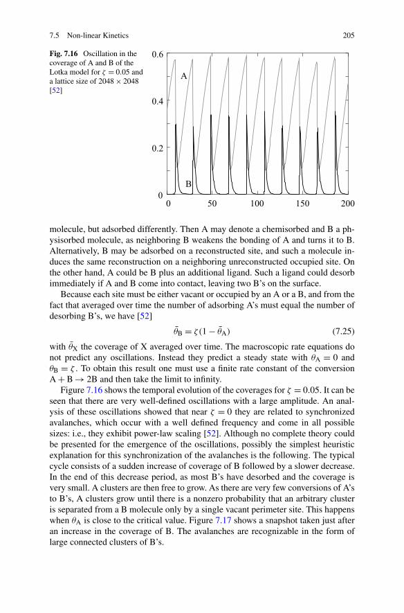
7.5 Non-linear Kinetics 205

Fig. 7.16 Oscillation in thecoverage of A and B of theLotka model for ζ = 0.05 anda lattice size of 2048 × 2048[52]

molecule, but adsorbed differently. Then A may denote a chemisorbed and B a ph-ysisorbed molecule, as neighboring B weakens the bonding of A and turns it to B.Alternatively, B may be adsorbed on a reconstructed site, and such a molecule in-duces the same reconstruction on a neighboring unreconstructed occupied site. Onthe other hand, A could be B plus an additional ligand. Such a ligand could desorbimmediately if A and B come into contact, leaving two B’s on the surface.

Because each site must be either vacant or occupied by an A or a B, and from thefact that averaged over time the number of adsorbing A’s must equal the number ofdesorbing B’s, we have [52]

θB = ζ(1 − θA) (7.25)

with θX the coverage of X averaged over time. The macroscopic rate equations donot predict any oscillations. Instead they predict a steady state with θA = 0 andθB = ζ . To obtain this result one must use a finite rate constant of the conversionA + B → 2B and then take the limit to infinity.

Figure 7.16 shows the temporal evolution of the coverages for ζ = 0.05. It can beseen that there are very well-defined oscillations with a large amplitude. An anal-ysis of these oscillations showed that near ζ = 0 they are related to synchronizedavalanches, which occur with a well defined frequency and come in all possiblesizes: i.e., they exhibit power-law scaling [52]. Although no complete theory couldbe presented for the emergence of the oscillations, possibly the simplest heuristicexplanation for this synchronization of the avalanches is the following. The typicalcycle consists of a sudden increase of coverage of B followed by a slower decrease.In the end of this decrease period, as most B’s have desorbed and the coverage isvery small. A clusters are then free to grow. As there are very few conversions of A’sto B’s, A clusters grow until there is a nonzero probability that an arbitrary clusteris separated from a B molecule only by a single vacant perimeter site. This happenswhen θA is close to the critical value. Figure 7.17 shows a snapshot taken just afteran increase in the coverage of B. The avalanches are recognizable in the form oflarge connected clusters of B’s.

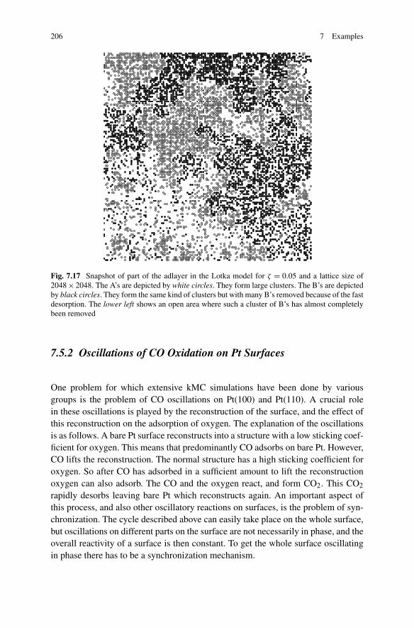
206 7 Examples

Fig. 7.17 Snapshot of part of the adlayer in the Lotka model for ζ = 0.05 and a lattice size of2048 × 2048. The A’s are depicted by white circles. They form large clusters. The B’s are depictedby black circles. They form the same kind of clusters but with many B’s removed because of the fastdesorption. The lower left shows an open area where such a cluster of B’s has almost completelybeen removed

7.5.2 Oscillations of CO Oxidation on Pt Surfaces

One problem for which extensive kMC simulations have been done by variousgroups is the problem of CO oscillations on Pt(100) and Pt(110). A crucial rolein these oscillations is played by the reconstruction of the surface, and the effect ofthis reconstruction on the adsorption of oxygen. The explanation of the oscillationsis as follows. A bare Pt surface reconstructs into a structure with a low sticking coef-ficient for oxygen. This means that predominantly CO adsorbs on bare Pt. However,CO lifts the reconstruction. The normal structure has a high sticking coefficient foroxygen. So after CO has adsorbed in a sufficient amount to lift the reconstructionoxygen can also adsorb. The CO and the oxygen react, and form CO2. This CO2

rapidly desorbs leaving bare Pt which reconstructs again. An important aspect ofthis process, and also other oscillatory reactions on surfaces, is the problem of syn-chronization. The cycle described above can easily take place on the whole surface,but oscillations on different parts on the surface are not necessarily in phase, and theoverall reactivity of a surface is then constant. To get the whole surface oscillatingin phase there has to be a synchronization mechanism.

7.5 Non-linear Kinetics 207

Fig. 7.18 Global oscillations and pattern formation with D = 250. The top shows temporal varia-tions of the coverages, the fraction of the substrate in the α phase, and the CO2 production R. Eachpicture has two parts. In the left part we plot the chemical species: CO particles are gray and Oparticles are white, and vacant sites are black. The right part shows the structure of the surface: α

phase sites are black, and β phase sites are white. Sections of the upper-left corner with L = 8192,4096, 1024, and 256 are shown on the left half of the figure. The sections correspond to the dot inthe temporal plot at the top. On the right half of the figure we have a wave front, a target, a spiral,and turbulence (L = 2048), which can be obtained with different initial conditions [51]

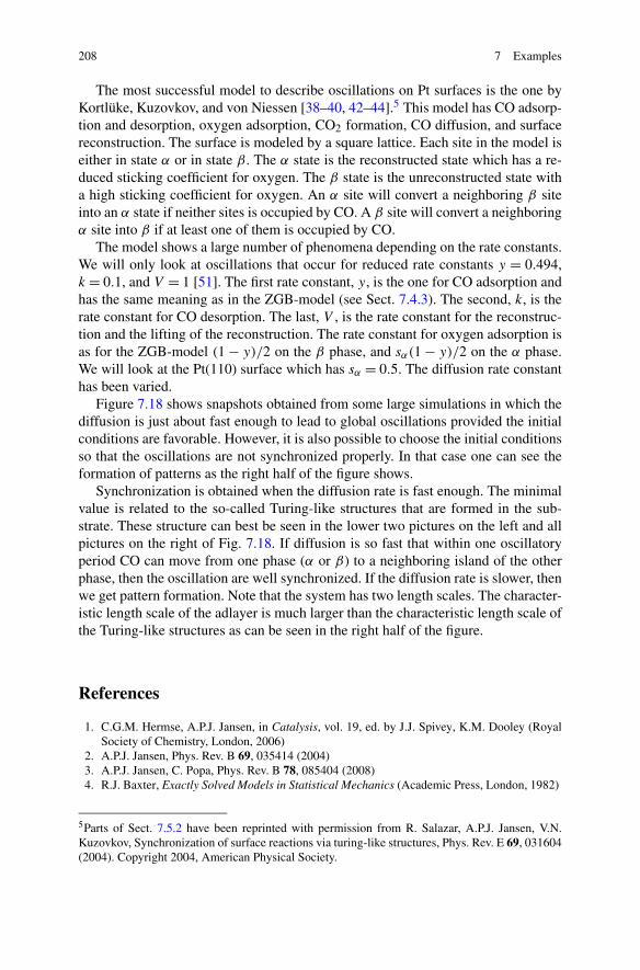
208 7 Examples

The most successful model to describe oscillations on Pt surfaces is the one byKortlüke, Kuzovkov, and von Niessen [38–40, 42–44].5 This model has CO adsorp-tion and desorption, oxygen adsorption, CO2 formation, CO diffusion, and surfacereconstruction. The surface is modeled by a square lattice. Each site in the model iseither in state α or in state β . The α state is the reconstructed state which has a re-duced sticking coefficient for oxygen. The β state is the unreconstructed state witha high sticking coefficient for oxygen. An α site will convert a neighboring β siteinto an α state if neither sites is occupied by CO. A β site will convert a neighboringα site into β if at least one of them is occupied by CO.

The model shows a large number of phenomena depending on the rate constants.We will only look at oscillations that occur for reduced rate constants y = 0.494,k = 0.1, and V = 1 [51]. The first rate constant, y, is the one for CO adsorption andhas the same meaning as in the ZGB-model (see Sect. 7.4.3). The second, k, is therate constant for CO desorption. The last, V , is the rate constant for the reconstruc-tion and the lifting of the reconstruction. The rate constant for oxygen adsorption isas for the ZGB-model (1 − y)/2 on the β phase, and sα(1 − y)/2 on the α phase.We will look at the Pt(110) surface which has sα = 0.5. The diffusion rate constanthas been varied.

Figure 7.18 shows snapshots obtained from some large simulations in which thediffusion is just about fast enough to lead to global oscillations provided the initialconditions are favorable. However, it is also possible to choose the initial conditionsso that the oscillations are not synchronized properly. In that case one can see theformation of patterns as the right half of the figure shows.

Synchronization is obtained when the diffusion rate is fast enough. The minimalvalue is related to the so-called Turing-like structures that are formed in the sub-strate. These structure can best be seen in the lower two pictures on the left and allpictures on the right of Fig. 7.18. If diffusion is so fast that within one oscillatoryperiod CO can move from one phase (α or β) to a neighboring island of the otherphase, then the oscillation are well synchronized. If the diffusion rate is slower, thenwe get pattern formation. Note that the system has two length scales. The character-istic length scale of the adlayer is much larger than the characteristic length scale ofthe Turing-like structures as can be seen in the right half of the figure.

References

1. C.G.M. Hermse, A.P.J. Jansen, in Catalysis, vol. 19, ed. by J.J. Spivey, K.M. Dooley (RoyalSociety of Chemistry, London, 2006)

2. A.P.J. Jansen, Phys. Rev. B 69, 035414 (2004)3. A.P.J. Jansen, C. Popa, Phys. Rev. B 78, 085404 (2008)4. R.J. Baxter, Exactly Solved Models in Statistical Mechanics (Academic Press, London, 1982)

5Parts of Sect. 7.5.2 have been reprinted with permission from R. Salazar, A.P.J. Jansen, V.N.Kuzovkov, Synchronization of surface reactions via turing-like structures, Phys. Rev. E 69, 031604(2004). Copyright 2004, American Physical Society.

References 209

5. H.J. Borg, J.F.C.J.M. Reijerse, R.A. van Santen, J.W. Niemantsverdriet, J. Chem. Phys. 101,10052 (1994)

6. R.M. van Hardeveld, M.J.P. Hopstaken, J.J. Lukkien, P.A.J. Hilbers, A.P.J. Jansen, R.A. vanSanten, J.W. Niemantsverdriet, Chem. Phys. Lett. 302, 98 (1999)

7. D. Loffreda, D. Simon, P. Sautet, J. Chem. Phys. 108, 6447 (1998)8. D. Loffreda, D. Simon, P. Sautet, J. Catal. 213, 211 (2003)9. C.G.M. Hermse, F. Frechard, A.P. van Bavel, J.J. Lukkien, J.W. Niemantsverdriet, R.A. van

Santen, A.P.J. Jansen, J. Chem. Phys. 118, 7081 (2003)10. A.P.J. Jansen, C.G.M. Hermse, F. Fréchard, J.J. Lukkien, in Computational Science—ICCS

2001, ed. by V. Alexandrov, J. Dongarra, B. Juliano, R. Renner, C. Tan (Springer, Berlin,2001), pp. 531–540

11. C.T. Kao, G.S. Blackman, M.A.V. Hove, G.A. Somorjai, C.M. Chan, Surf. Sci. 224, 77 (1989)12. I. Zasada, M.A.V. Hove, G.A. Somorjai, Surf. Sci. 418, L89 (1998)13. K.B. Rider, K.S. Hwang, M. Salmeron, G.A. Somorjai, Phys. Rev. Lett. 86, 4330 (2001)14. M.T.M. Koper, J.J. Lukkien, A.P.J. Jansen, R.A. van Santen, J. Phys. Chem. B 103, 5522

(1999)15. M. Flytzani-Stephanopoulos, L.D. Schmidt, Prog. Surf. Sci. 9, 83 (1979)16. T.C. Wei, J. Phillips, Adv. Catal. 41, 359 (1996)17. D.W. Blakely, G.A. Somorjai, Surf. Sci. 65, 419 (1977)18. X.Q. Zhang, W.K. Offermans, R.A. van Santen, A.P.J. Jansen, A. Scheibe, U. Lins, R. Imbihl,

Phys. Rev. B 82, 113401 (2010)19. E. Shustorovich, Surf. Sci. Rep. 6, 1 (1986)20. W.K. Offermans, A.P.J. Jansen, R.A. van Santen, G. Novell-Leruth, J.M. Ricart, J. Pérez-

Ramirez, J. Phys. Chem. C 111, 17551 (2007)21. S. Wiggins, Introduction to Applied Nonlinear Dynamical Systems and Chaos (Springer, New

York, 1990)22. J.K. Hale, H. Koçak, Dynamics and Bifurcations (Springer, New York, 1991)23. M.M. Slin’ko, N.I. Jaeger, Oscillating Heterogeneous Catalytic Systems. Studies in Surface

Science and Catalysis, vol. 86 (Elsevier, Amsterdam, 1994)24. R. Imbihl, G. Ertl, Chem. Rev. 95, 697 (1995)25. Q. Ge, R. Kose, D.A. King, Adv. Catal. 45, 207 (2000)26. M.T.M. Koper, J. Electroanal. Chem. 450, 189 (1998)27. M.T.M. Koper, A.P.J. Jansen, J.J. Lukkien, Electrochim. Acta 45, 645 (1999)28. J. Clavilier, in Interfacial Electrochemistry, Theory, Experiment and Applications, ed. by

A. Wieckowski (Dekker, New York, 1999), pp. 231–24829. B.M. Ocko, J.X. Wang, T. Wandlowski, Phys. Rev. Lett. 79, 1511 (1997)30. A.M. Funtikov, U. Stimming, R. Vogel, J. Electroanal. Chem. 428, 147 (1997)31. C.G.M. Hermse, A.P. van Bavel, M.T.M. Koper, J.J. Lukkien, R.A. van Santen, A.P.J. Jansen,

Surf. Sci. 572, 247 (2004)32. J.M. Orts, L. Blum, D. Huckaby, J.M. Feliu, A. Aldaz, Abstr. Pap. Am. Chem. Soc. 220, 91

(2000)33. R.M. Ziff, E. Gulari, Y. Barshad, Phys. Rev. Lett. 56, 2553 (1986)34. H.P. Kaukonen, R.M. Nieminen, J. Chem. Phys. 91, 4380 (1989)35. J.P. Hovi, J. Vaari, H.P. Kaukonen, R.M. Nieminen, Comput. Mater. Sci. 1, 33 (1992)36. J. Mai, A. Casties, W. von Niessen, V.N. Kuzovkov, J. Chem. Phys. 102, 5037 (1995)37. R.J. Gelten, A.P.J. Jansen, R.A. van Santen, J.J. Lukkien, J.P.L. Segers, P.A.J. Hilbers,

J. Chem. Phys. 108, 5921 (1998)38. V.N. Kuzovkov, O. Kortlüke, W. von Niessen, Phys. Rev. Lett. 83, 1636 (1999)39. O. Kortlüke, V.N. Kuzovkov, W. von Niessen, Phys. Rev. Lett. 83, 3089 (1999)40. V.N. Kuzovkov, O. Kortlüke, W. von Niessen, Phys. Rev. E 66, 011603 (2002)41. R.J. Gelten, R.A. van Santen, A.P.J. Jansen, in Molecular Dynamics: From Classical to Quan-

tum Methods, ed. by P.B. Balbuena, J.M. Seminario (Elsevier, Amsterdam, 1999), pp. 737–784

42. O. Kortlüke, V.N. Kuzovkov, W. von Niessen, Phys. Rev. Lett. 81, 2164 (1998)

210 7 Examples

43. V.N. Kuzovkov, O. Kortlüke, W. von Niessen, J. Chem. Phys. 108, 5571 (1998)44. O. Kortlüke, V.N. Kuzovkov, W. von Niessen, J. Chem. Phys. 110, 11523 (1999)45. A.P.J. Jansen, R.M. Nieminen, J. Chem. Phys. 106, 2038 (1997)46. A.P.J. Jansen, J. Mol. Catal. A, Chem. 119, 125 (1997)47. R.M. Ziff, B.J. Brosilow, Phys. Rev. A 46, 4630 (1992)48. B.J. Brosilow, E. Gulari, R.M. Ziff, J. Chem. Phys. 98, 674 (1993)49. I. Jensen, H. Fogedby, R. Dickman, Phys. Rev. A 41, 3411 (1990)50. P. Grindrod, The Theory and Applications of Reaction-Diffusion Equations: Patterns and

Waves (Clarendon, Oxford, 1996)51. R. Salazar, A.P.J. Jansen, V.N. Kuzovkov, Phys. Rev. E 69, 031604 (2004)52. J.P. Hovi, A.P.J. Jansen, R.M. Nieminen, Phys. Rev. E 55, 4170 (1997)53. J. Mai, V.N. Kuzovkov, W. von Niessen, A Lotka type model for oscillations in surface reac-

tions (1995). Private communication54. J. Mai, V.N. Kuzovkov, W. von Niessen, Oscillations beyond the mean-field description: The

Lotka model (1995). Private communication

Chapter 8New Developments

Abstract Kinetic Monte Carlo (kMC) is a very versatile and powerful methodto study the kinetics of surface reactions, but there are nevertheless some systemsand phenomena for which one would like it to be more efficient or one wouldlike to extend it. We discuss what kind of fast processes may pose a problem,when they become problematic, and what can be done about it so that kMC sim-ulations can be done with longer time scales. Coarse-graining is presented as amethod to do simulations with larger length scales. Mass transport and heat transferare discussed in the context of continuum models that are coupled to kMC sim-ulations. Finally, off-lattice kMC simulations are introduced to show that one canalso do kMC simulations of systems that can not be described with a lattice-gasmodel.

8.1 Longer Time Scales and Fast Processes

In many simulations the period that one has to simulate a system is determined byhow long it takes the system to reach the state of interest (e.g., a steady state), andthe time one needs to simulate the system to get good statistics for the results. Nei-ther times are generally very long. There are exceptions however. Relaxation timessometimes are long, or one is interested in processes with intrinsically long timescales: e.g., time-dependent experiments like Temperature-Programmed Desorptionor oscillations. It is not always possible to get to the time scale of interest with aconventional kinetic Monte Carlo (kMC) simulation.

Even if the real time that one wants to simulate a system is not long, a simulationmay still take a lot of computer time because some of the processes are very fast. Thecomputer time is determined by the number of processes that actually take place. Asthis number also determines if one has good statistics, one might assume that withfaster processes one need not simulate a system so long. That is correct, exceptwhen there are both fast and slow processes in the system. To get good statistics onthe slow processes one then needs to simulate an inordinate large number of fastprocesses.

A.P.J. Jansen, An Introduction to Kinetic Monte Carlo Simulations of SurfaceReactions, Lecture Notes in Physics 856,DOI 10.1007/978-3-642-29488-4_8, © Springer-Verlag Berlin Heidelberg 2012

211

212 8 New Developments

8.1.1 When Are Fast Processes a Problem?

The theory of kMC does not pose any restrictions on the rate constants of the pro-cesses being simulated. So there is no fundamental problem when there are pro-cesses in a reaction system with very dissimilar rate constants. However, fast pro-cesses can make a simulations slow and inefficient.

First, there is the question of which algorithm to use. This is discussed in Chap. 3.The problem is oversampling, which can become very inefficient with rate constantsthat differ a lot. The First Reaction Method (FRM) has no problems at all with fastprocesses because there is no oversampling, but the Random Selection Method willonly rarely work well. The Variable Step Size Method (VSSM) works well if nooversampling is used, but otherwise may be inefficient. The procedure in Sect. 3.9can be used to show rapidly which algorithm works best.

A different problem, one not so easily solved, is when almost all processes thatactual take place in a system are fast processes but one is really interested in thefew slow ones. This is for example quite common when one is interested in thechemical reactions on a catalyst’s surface, but most processes are diffusional hopsof the adsorbates. A kMC simulation will then spend almost all time on diffusionwhatever the algorithm one uses.

It is important to understand the precise nature of the problem. A fast processin itself is not a problem For example, suppose that a molecule has a high rateconstant for adsorption. The consequence of this is that a molecule will adsorb assoon as there is a vacancy. The number of such adsorption process will remain small,because adsorption will stop when all vacancies are occupied. It only becomes aproblem if the molecules also have a high rate constant for desorption. In that casenew vacancies will be formed with a high rate, and a simulation ends up in spendingall time simulating an adsorption-desorption equilibrium. There is also no problemif only the rate constant for desorption is high, because then the number of processesis limited by the slow adsorption. Of course, there will not be many molecules onthe surface, but that is as it should be, as it is a consequence of the nature of theadsorption-desorption equilibrium.

So there will only be problems with fast processes if a fast process can be fol-lowed by infinite many other fast processes. Adsorption-desorption is one example.Another would be a fast reaction that also has a fast reverse reaction. The mostcommon case is however fast diffusion.

8.1.2 A Simple Solution

The simplest approach is to reduce the rate constants of all fast processes involvedby some constant factor. This is the same as increasing the energies of the transi-tion states of these processes by the same amount. The idea is that what all theseprocesses do is to equilibrate a subset of all configurations. This equilibration can

8.1 Longer Time Scales and Fast Processes 213

however also be accomplished with much smaller rate constants. The pragmatic ap-proach is then to start with a very large reduction of the rate constants: so large,that the fast processes no longer dominate the time it takes to do a simulation. Thenone should increase the rate constants and look at how the results of the simulationchange. At a certain point the results will converge as a function of these rate con-stants. At this point the simulation yields the same results as a simulation with thereal rate constants, but with minimal computer time. We have noticed that in thecase of diffusion this approach can easily speed up a simulation by three or moreorders of magnitude. Note that reducing the rate constants of the fast processes doesnot slow down the evolution of the system because this is determined by the slowprocesses. The same behavior is seen but with fewer fast processes.

The idea of reducing the rate constants has been worked out and automated byChatterjee and Voter in their Accelerated Superbasin kMC [1]. The approach keepstrack of how often configurations are revisited. If this occurs often, then this is in-dicative of the system being trapped in a set of configurations connected by fastprocesses. This is the superbasin of the approach. The energies of the transitionstates of these fast processes is then increased. Depending on how much that theseenergies are changes, the procedure may have to be repeated a number of times untilthe fast processes are slowed down so much that an escape from the superbasin oc-curs. Chatterjee and Voter give criteria to determine when a revisit is indeed pointingto the existence of a superbasin.

Changing the rate constants as described here introduces no errors in the prob-abilities of the configurations if the system is in equilibrium. The energies of tran-sition states do not determine or affect equilibrium properties in any way. Manysituations exist however for surface reactions where there is an irreversible process:e.g., the desorption of a molecule that has been created on the surface. In these sit-uations the system is not in equilibrium, but at steady state. Forward and reversereactions have different rates in such a system, and the difference is proportional tothe overall reactivity. Changing the energies of the transition states changes initiallythe rates of forward and reverse reactions by the same factor, and that changes theirdifference as well. As a consequence the coverages and the reactivity will subse-quently change as well, and the behavior of the system is no longer the same. Ingeneral, this effect is small if only transition states of fast processes are changed,and the approach then is a good approximation.

8.1.3 Reduced Master Equations

A more sophisticated approach using the same equilibration idea is to remove thefast processes completely. Let C(α) be the set of all configurations that can bereached from configuration α by some fast processes only. We can partition all con-figurations in such sets. Let PC(α) be the probability that the system is in one of theconfigurations of C(α): i.e.,

PC(α) =∑

α′∈C(α)

Pα′ . (8.1)

214 8 New Developments

We then havedPC(α)

dt=∑

C(β)

[ΩC(α)C(β)PC(β) − ΩC(β)C(α)PC(α)] (8.2)

with the new rate constants

ΩC(α)C(β) =∑

α′∈C(α)

∑

β ′∈C(β)

Wα′β ′Pβ ′

PC(β)

. (8.3)

This equation is again a master equation provided that all Pβ ′/PC(β) are constant,which they are for infinitely fast processes. The reason is that such fast processesbring all β ′ ∈ C(β) to equilibrium instantaneously and the ratio is nothing but aconditional probability that the system is in β ′ given that it is in one of the configu-rations of C(β). This ratio is determined by the fast processes only.

The applicability of Eq. (8.2) depends a how easily Pβ ′/PC(β) can be deter-mined. For diffusion in a one-dimensional zeolite this proved to be easy, and insteadof a master equation with configurations a master equations with the numbers ofmolecules could be used [2]. For higher dimensional system things might not be soeasy.

To get Pβ ′/PC(β) in the general case, one has to solve∑

β ′′∈C(β)

[Wβ ′β ′′Pβ ′′ − Wβ ′′β ′Pβ ′ ] = 0 (8.4)

with β ′ ∈ C(β) and subject to the restriction∑

β ′∈C(β)

Pβ ′ = PC(β). (8.5)

We can remove the need to know PC(β) by rewriting this as

∑

β ′′∈C(β)

[Wβ ′β ′′

Pβ ′′

PC(β)

− Wβ ′′β ′Pβ ′

PC(β)

]= 0 (8.6)

with the restriction∑

β ′∈C(β)

Pβ ′

PC(β)

= 1. (8.7)

This does not yield the Pβ ′ ’s, but only the Pβ ′/PC(β)’s, but that is also really all weneed to know.

Equations (8.6) and (8.7) form a set of linear equations that need to be solved. Inthe case of the one-dimensional zeolite mentioned above this could be done analyt-ically [2], but if this is not possible one has to hope that the number of equations,which equals the number of configurations in C(β), is not too large.

Mastny et al. have used this reduced master equation (8.3) for a simple modelof CO oxidation [3]. They have defined the sets C(α) as all configurations with thesame number of adsorbates of each type just as was done for the one-dimensionalzeolite. They have tried two approaches to solve Eq. (8.6). In the first they used very

8.1 Longer Time Scales and Fast Processes 215

small lattices (5 × 5 or 10 × 10). With these lattices there are only several hundredsto several thousands equations (8.3) and the rate constants for all of them weredetermined by doing normal but short kMC simulations with these small lattices.Only diffusion of the adsorbates was included in these simulations. The probabilitythat a certain configuration β was found in such a simulation was then equal toPβ/PC(β), and that information was then used to compute ΩC(α)C(β) via Eq. (8.3).

Their second approach consisted of a derivation of the exact rate equations for thecoverages (see Sect. 4.6). The coverage dependence of the rates was then determinedusing kMC simulations with large lattices, but again also with only diffusion. Insteadof investigating all possible combinations of the number of adsorbates, which wouldnot have been possible, they looked at a discrete sampling of coverages and theninterpolated.

Both approaches were shown to give good results. An advantage of both ap-proaches is that it is much easier to study how the behavior of a system depends onthe rate constants of the processes than with kMC. The reason is that the effect ofthe diffusion can be determined independently from that of the other processes: i.e.,the kMC simulations with only diffusion need to be done only once and the resultscan be used in all subsequent simulations or calculations.

8.1.4 Dealing with Slightly Slower Reactions

A more sophisticated approach was introduced by Mason et al. in their work onflicker processes [4, 5]. It has the advantage that it can also be used when there isnot such a clearcut distinction between fast and slow processes, although the extracomputational costs of the more complicated algorithm may not be worthwhile ifthe “fast” processes become too slow. A flicker process is change α → β of config-urations immediately followed by the reverse change β → α. In their work Mason etal. grouped all changes α → β → α for a fixed α and all possible β’s, and computeda time when the chain of flicker processes is broken. They also determined whichconfiguration the system then goes to. Consequently, the flicker processes need nolonger be simulated explicitly which can speed up a simulation substantially.

8.1.4.1 The General Case

We will first discuss a more general situation. Suppose at time t = 0 we are at con-figuration α0 and there are a number of processes that we consider fast, that we donot want to simulate explicitly, and that can bring the system to a set of configu-rations C(α0). We also define the complement K(α0) of C(α0), which contains allconfigurations not in C(α0). The situation is sketched in Fig. 8.1. We want to knowfirst what the first configuration in K(α0) will be when the system moves outsideC(α0). We want to know second at what time this will occur. And third, we want analgorithm that can generate this information.

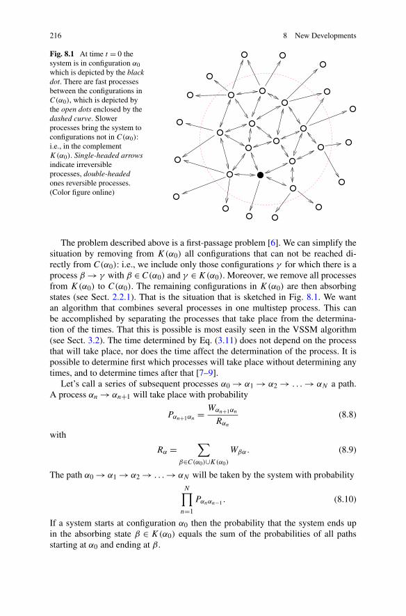
216 8 New Developments

Fig. 8.1 At time t = 0 thesystem is in configuration α0which is depicted by the blackdot. There are fast processesbetween the configurations inC(α0), which is depicted bythe open dots enclosed by thedashed curve. Slowerprocesses bring the system toconfigurations not in C(α0):i.e., in the complementK(α0). Single-headed arrowsindicate irreversibleprocesses, double-headedones reversible processes.(Color figure online)

The problem described above is a first-passage problem [6]. We can simplify thesituation by removing from K(α0) all configurations that can not be reached di-rectly from C(α0): i.e., we include only those configurations γ for which there is aprocess β → γ with β ∈ C(α0) and γ ∈ K(α0). Moreover, we remove all processesfrom K(α0) to C(α0). The remaining configurations in K(α0) are then absorbingstates (see Sect. 2.2.1). That is the situation that is sketched in Fig. 8.1. We wantan algorithm that combines several processes in one multistep process. This canbe accomplished by separating the processes that take place from the determina-tion of the times. That this is possible is most easily seen in the VSSM algorithm(see Sect. 3.2). The time determined by Eq. (3.11) does not depend on the processthat will take place, nor does the time affect the determination of the process. It ispossible to determine first which processes will take place without determining anytimes, and to determine times after that [7–9].

Let’s call a series of subsequent processes α0 → α1 → α2 → . . . → αN a path.A process αn → αn+1 will take place with probability

Pαn+1αn = Wαn+1αn

Rαn

(8.8)

with

Rα =∑

β∈C(α0)∪K(α0)

Wβα. (8.9)

The path α0 → α1 → α2 → . . . → αN will be taken by the system with probabilityN∏

n=1

Pαnαn−1 . (8.10)

If a system starts at configuration α0 then the probability that the system ends upin the absorbing state β ∈ K(α0) equals the sum of the probabilities of all pathsstarting at α0 and ending at β .

8.1 Longer Time Scales and Fast Processes 217

The evaluation of this sum can most easily be computed with a transition matrixP defined by

Pαj αi= Pαj αi

(8.11)

with αj ,αi ∈ C(α0). The matrix elements of P can be interpreted as the probabilitiesof paths that consist of only a single process. From

(P2)

αj αi=∑

αk

Pαj αkPαkαi

(8.12)

we see that P2 has the probabilities of paths consisting of two processes startingand ending at configurations of C(α0). Similarly Pn has the probabilities of pathsconsisting of n processes starting and ending at configurations of C(α0). Now theprobability that the system starts at α0 and ends up in β ∈ K(α0) after n processesin C(α0) equals

∑

α∈C(α0)

Pβα(Pn)αα0 . (8.13)

The probabilities that the system exits C(α0) after n processes is obtained by sum-ming over all β ∈ K(α0). These probabilities allow us to determine the number ofprocesses that take place in C(α0) before the system exits C(α0), and the probabil-ities for the configurations in K(α0) the system then goes to.

Now suppose that we are also able to determine the precise path that the systemtakes in C(α0), then the time when the system exits C(α0) can be determined asfollows. Let the path be α0 → α1 → α2 → . . . → αn → β . The time it takes for allprocesses in this path to occur is then

n∑

m=0

Δtm (8.14)

with Δtm a random number taken from the probability distribution

Rαm exp[−Rαmt]. (8.15)

The algorithm is then as follows

1. Determine the number of processes in C(α0) before the system exits C(α0) bysumming over the configurations β in Eq. (8.13).

2. Determine the configuration β ∈ K(α0) that the system moves to after exitingC(α0). Use again Eq. (8.13).

3. Determine the path from α0 to β with the correct number of processes.4. Determine the time that it takes to follow this path. Use Eq. (8.14).

Steps 1 and 2 are selections that can be done with one of the procedures discussedin Sect. 3.3.1. See also Sect. 8.1.4.5. Step 3 has not been discussed yet. In general itis a very complicated problem. So we will discuss only the most common cases butwith all steps in detail.

218 8 New Developments

Fig. 8.2 The threeconfigurations involved infast adsorption-desorptionwith a slower reaction of theadsorbed species. V standsfor a vacant adsorption site, Afor the adsorbed species, and∗ for the absorbing state withthe species that has reacted

8.1.4.2 Adsorption-Desorption

Suppose we have a single adsorption site and an adsorbate with high adsorption anddesorption rate constants. Figure 8.2 shows the three configurations involved. Wehave an adsorption rate constant Wads changing V to A, a desorption rate constantWdes changing A to V, and a reaction rate constant Wrx for the reaction A → ∗. Ourapproach is useful if Wads,Wdes � Wrx, but it is also correct if this inequality doesnot hold. From the rate constants we can derive the probabilities of the processes

Pads = 1, (8.16)

Pdes = Wdes

Wdes + Wrx, (8.17)

and

Prx = Wrx

Wdes + Wrx. (8.18)

The transition matrix P then becomes

P =(

0 Pdes1 0

)(8.19)

with the states ordered V, A. It is easy then to derive

P2n = P ndes

(1 00 1

)(8.20)

and

P2n+1 = P ndes

(0 Pdes1 0

). (8.21)

We start in configuration V. The probability that the reaction to ∗ takes place afteradsorption V → A, and n adsorption-desorption cycles A → V → A, is then

(P2n+1)

AVPrx = P ndesPrx. (8.22)

We note that these probabilities are properly normalized as

∞∑

n=0

P ndesPrx = Prx

1 − Pdes= 1. (8.23)

8.1 Longer Time Scales and Fast Processes 219

Fig. 8.3 Fast reactions fromA to one of the Vn’s and backoccur repeatedly before thesystem converts to ∗. Allprocesses A → Vn have thesame rate constant WA→V.All processes Vn → A havethe rate constant WV→A. Theconversion to ∗ has rateconstant WA→∗

We can use these probabilities to generate the number of cycles A → V → A thattake place before the reaction occurs with one the selection methods in Sect. 3.3.1.

To determine when the reaction takes place is easy in this case, because giventhe number n of cycles A → V → A it is clear what path the system takes. With n

such cycles there are n+1 adsorptions, n desorptions, and one reaction. So we needto generate n + 1 intervals Δt from the probability distribution Wads exp[−WadsΔt]and also n+ 1 intervals from (Wdes +Wrx) exp[−(Wdes +Wrx)Δt]. If we add up allthese intervals, we get the time when the reaction takes place if we start in V at timet = 0. Note that the intervals for the desorption and the reaction are taken from thesame distribution, because they occur in the same configuration A.

If we don’t have one adsorption site but many, then we can regard the adsorption,the desorption-adsorption cycles, and the reaction at each site as one multistep pro-cess, determine a time for each of them, and use FRM to determine which multistepprocess occurs first and to do the simulation (see Sect. 3.5). This avoids a muchlarger matrix P describing all possible occupations of the various sites.

The adsorption-desorption process above can easily be extended to the flickerprocesses studied by Mason et al. [4]. Figure 8.3 shows multiple configurations towhich the system can convert from and to A. (We use a notation similar to the oneof the adsorption-desorption case, but change the meaning.) This is essentially thesame process as adsorption-desorption except that the rate constant Wads should bereplaced by NWV→A and Wdes by NWA→V.

8.1.4.3 Fast Equilibrium

Suppose we have a fast conversion reaction A → B and a fast reverse B → A on asingle site. Also suppose that there are two slower reactions: A → X and B → Y(see Fig. 8.4). The important difference with the cases above is that there are twoways in which the cycles of fast reactions A → B → A can end. The additional

220 8 New Developments

Fig. 8.4 The fourconfigurations involved in afast equilibrium with slowerreactions of both species inthe equilibrium. A and B arethe species of the equilibrium.A converts slowly to X, and Bslowly to Y

question then is what the probabilities are for ending at X or Y. The P matrix hasthe following form.

P =(

0 PB→APA→B 0

)(8.24)

with

PA→B = WA→B

WA→B + WA→X(8.25)

and

PB→A = WB→A

WB→A + WB→Y. (8.26)

We have

P2n = (PA→BPB→A)n(

1 00 1

)(8.27)

and

P2n+1 = (PA→BPB→A)n(

0 PB→APA→B 0

). (8.28)

If we start at A, then the probability to end at X after n cycles A → B → A equals

(PA→BPB→A)nPA→X (8.29)

with

PA→X = WA→X

WA→B + WA→X. (8.30)

The probability to end at Y after A → B and n cycles B → A → B equals

PA→B(PB→APA→B)nPB→Y (8.31)

with

PB→Y = WB→Y

WB→A + WB→Y. (8.32)

We have

8.1 Longer Time Scales and Fast Processes 221

Fig. 8.5 A collection of adsorption sites for a CO molecule. The molecule can hop between neigh-boring sites. The open dots depict sites at which the molecule can react with an oxygen atom toform CO2. At time t = 0 the CO molecule is assumed to have adsorbed at the site indicated by thearrow. The large square centered at this site is an example of a protective domain. (Color figureonline)

∞∑

n=0

(PA→BPB→A)nPA→X +∞∑

n=0

PA→B(PB→APA→B)nPB→Y

= PA→X

1 − PA→BPB→A+ PA→BPB→Y

1 − PB→APA→B

= (1 − PA→B) + (1 − PB→A)PA→B

1 − PA→BPB→A= 1 (8.33)

as it should be. We also see that the probability to end up at X equals PA→X/(1 −PA→BPB→A) and the probability to end up at Y equals PA→BPB→Y/(1 −PB→APA→B).

The times it takes to end at X or Y after a number of cycles are sums ofintervals taken from the probability distributions fA(Δt) = (WA→B + WA→X) ×exp[−(WA→B + WA→X)Δt] and fB(Δt) = (WB→A + WB→Y) exp[−(WB→A +WB→Y)Δt]. To end up at X after n cycles A → B → A takes n + 1 intervals fromfA and n intervals from fB. To end up at Y after A → B and n cycles B → A → Btakes n + 1 intervals from fA and n + 1 intervals from fB.

8.1.4.4 Fast Diffusion

The analytical approaches for adsorption-desorption and fast equilibria are not al-ways possible for diffusion. To see the problem let’s look at a simple model. Sup-pose we have a single CO molecule that can hop between a number of sites. Someof these sites are next to sites occupied with oxygen atoms. If the CO molecule is atsuch a site, it can react with on oxygen atom to form CO2. The situation is sketchedin Fig. 8.5 for a square lattice of adsorption sites.

The problem is that, because of the irregular shape of the set of sites that CO canhop to, it will be very hard to derive expressions for finding CO at the edge sites

222 8 New Developments

where it can react with oxygen. Of course, it is possible to set up a transition matrixP as in Eqs. (8.11) to (8.13), but it is doubtful that explicit use of such a matrixis really more efficient than a standard kMC simulation. Moreover, the matricesPn may give the probabilities of finding the CO molecule at different sites after anumber of steps, but that still leaves the problem of determining the path. Note thateach site has a probability to hop to a particular neighboring site that depends on thenumber of neighbors. Also the time between hops depends on that number. Henceknowing the number of hops/steps in a path alone does not suffice for determiningthe time until the reaction.

Oppelstrup et al. have dealt with this problem by splitting the whole path inpieces, each of which can be treated analytically [10–12]. The idea is to define so-called protective domains (see Fig. 8.5). Inside such a domain the particle freelymoves and diffusion is the only process possible. The shape of the domain is suchthat the diffusion can be treated analytically. This is used to determine the time thatthe CO molecule reaches the boundary of the domain for the first time. (Hence thename for their method: first-passage kMC.) The system is then advanced to thattime. Then it is checked if the CO will react at its new site. If not, a new protectivedomain is defined and the procedure is repeated. Otherwise, CO will react and beremoved from the surface.

The example of CO diffusion and CO2 formation is really just a simple applica-tion of the method of Oppelstrup et al. [10–12]. They have extended their approachto many diffusing adsorbates that can react with each other. An important aspectof their approach is that in such situation it is not necessary to update the positionand protective domains of all adsorbates when one of them reaches the boundaryof its protective domain. Only the positions of that adsorbate and neighboring ad-sorbates need to be updated. This asynchronous algorithm makes the method size-independent and efficient.

The method works best if the protective domains are large, because then manydiffusional hops can be treated in one fell swoop. This is the case at low coverages.At high coverages and low reaction rate constants the method is not useful.

8.1.4.5 Algorithmic Aspects

Determining the number of reactions that take place in C(α0) before a configura-tion in K(α0) is reached is a selection problem (see Sect. 3.3.1). Suppose that theprobability that n steps take place in C(α0) equals Sn. We define the cumulativeprobability

Cn =n∑

m=0

Sm (8.34)

and a uniform deviate r ∈ [0,1). The number of steps n is given by

Cn−1 < r ≤ Cn (8.35)

with C−1 = 0 by definition.

8.1 Longer Time Scales and Fast Processes 223

It may be possible to do this selection easily by using the fact that there is asimple expression for Cn. For example, for the adsorption-desorption equilibriumcase (Sect. 8.1.4.2) the probability of the number of steps is given by PrxP

ndes with

n the number of A → V → A cycles. So the number of steps is 2n + 1 and S2n+1 =PrxP

ndes. We also have S2n = 0, because after 2n steps the system is in configuration

V from which no reaction is possible. Consequently

C2n = C2n+1 = Prx1 − P n+1

des

1 − Pdes. (8.36)

If we now look for Cn−1 < r ≤ Cn with r ∈ [0,1) a uniform deviate, then we caneasily determine n by solving

Prx1 − P

μ+1des

1 − Pdes= r (8.37)

for μ ∈ R. The number of cycles is simply the largest integer smaller or equal to μ.A similar solution can be found for the fast equilibrium (Sect. 8.1.4.3). Instead of

one summation, we have two: one for the paths that end up in X and one for thosethat end up in Y. We first do a simple selection for whether we end up in X or in Y,and then use a summation as for the adsorption-desorption case. For the situationof the fast diffusion the situation is not so easy however, because there is no simpleexpression for the probability of the number of processes in C(α0), and we need towork with Eq. (8.35).

The determination of the time when the system exits C(α0) has been presentedso far as a summation of the time intervals of all the individual processes. Whenthe number of these processes becomes large, this is a costly procedure. In fact, onemay wonder if treating the problem as a single multistep process is really so muchmore efficient than a normal kMC simulation. It is therefore useful to be able todetermine the time when the system exits C(α0) using a (hopefully small) numberof random number generations that does not depend on the number of processes inthe path in C(α0).

The examples above show that many of the time intervals are taken from the sameprobability distribution. We therefore will look here at the probability distributionof the sum

n∑

m=0

Δtm (8.38)

with all Δtm taken from the same probability distribution

P1(Δt) = We−WΔt . (8.39)

The subscript of P1 indicates that this is a probability distribution for a single pro-cess. For two subsequent processes we have

P2(Δt) =∫ Δt

0dτP1(Δt − τ)P1(τ ) = W 2

2Δte−WΔt . (8.40)

224 8 New Developments

Using

Pn+1(Δt) =∫ Δt

0dτP1(Δt − τ)Pn(τ ) (8.41)

it can be shown that

Pn(Δt) = Wn

n! Δtn−1e−WΔt . (8.42)

To determine the time tx that the system exits C(α0) after n processes we have tosolve

∫ tx

0dτPn(τ) = r (8.43)

with r a uniform deviate on the unit interval.For large n the integral in Eq. (8.43) does not yield a convenient expression.

Instead it seems better to use tabulation. We write∫ t

0dτPn(τ) = Wn

n!∫ t

0dττn−1e−Wτ = 1

n!∫ Wt

0dxxn−1e−x = πn(Wt) (8.44)

with

πn(τ) = 1

n!∫ τ

0dxxn−1e−x. (8.45)

So we compute and tabulate πn for many values of n and then use that tabulation tosolve Eq. (8.43).

8.1.5 Two Other Approaches

The time step in all of the algorithms that we have discussed so far, except the onein Sect. 3.7.1, is not under our control. This is sometimes a disadvantage: e.g., whenone wants to determine the temporal dependence of a probability distribution. Insuch a situation one would like to generate data at fixed points in time. Of course,one can use the fixed time step method of Sect. 3.7.1, but that is very inefficient.Moreover, the time step of that method is in general much smaller than the differencein time between two subsequent data sampling moments.

Kantorovich has investigated the possibility of an algorithm with a fixed largetime step [9]. Because the average times between the occurrence of two subsequentprocesses is generally smaller than the desired time step, this algorithm simulatesalso multistep processes. The difference between the approach in Sect. 8.1.4 is theway that the path of subsequent processes ends. In Sect. 8.1.4 this was determinedby the occurrence of a particular slow process. Here it is determined by the systemreaching a certain time.

The approach is based on the integral formulation of the master equation.

8.1 Longer Time Scales and Fast Processes 225

P(t) =[

Q(t,0) +∫ t

0dt ′Q

(t, t ′)W(t ′)Q(t ′,0

)

+∫ t

0dt ′∫ t ′

0dt ′′Q

(t, t ′)W(t ′)Q(t ′, t ′′

)W(t ′′)Q(t ′′,0

)+ . . .

]

× P(0) (8.46)

with

Q(t ′, t)= exp

[−∫ t ′

t

dt ′′R(t ′′)]

, (8.47)

Wαβ = Wαβ, (8.48)

and

Rαβ ={

0, if α = β,∑γ Wγβ, if α = β

(8.49)

(see Sects. 3.2.1 and 3.6). Note that this is the form for time-dependent rate con-stants. If the rate constants are time independent, then the argument of the matrix Wcan be left out and Q(t, t ′) depends only on the difference t − t ′ (see Sect. 3.2.1).The different terms on the right-hand-side of Eq. (8.46) stand for no processes tak-ing place between times 0 and t , one process taking place, two processes takingplace, et cetera.

Kantorovich proceeds by computing all of the contributions to P(t) analyticallyup to a preset maximum number of processes. This definitely yields the most de-tailed information on the evolution of the system, but it is very hard to do in general.By taking the time step not too large, the maximum number of processes can bechosen small, and the whole method may become feasible. However, it remains tobe seen how useful the method is from a practical point of view.

The τ -leap method also simulates many processes as one [13–15]. It was devel-oped for Dynamic Monte Carlo (DMC) simulations of rate equations, where onlyinformation on the total number of chemical species is used. The processes that aretaken together are assumed to be independent of each other: i.e., the occurrence ofone does not affect the others. In general, this is an approximation. It has been shownhowever that the errors thus introduced are negligible provided the relative changein the number of chemical species at each step is small [13]. This is the so-calledleap condition.

In normal lattice-gas kMC it seems impossible to fulfill this leap condition. A siteis either vacant or occupied and relative changes are always as large as they can be.Vlachos has tried to developed a method that leads to a much less restrictive leapcondition [16]. He groups all processes with the same rate constant together. Theτ -leap method is then applied to the processes in one group. The leap conditionthen becomes that the number of processes occurring in one time step must be smallcompared to the total number of processes in a group, but this number may still belarge.

The method has so far only been used for one system [16]. There it showedsubstantial savings in computer time. It was also noted however that the spatial in-formation in kMC, but absent in DMC, causes new problems for the τ -leap method.

226 8 New Developments

Fig. 8.6 Sketch of the coarse-graining of a lattice. The top-left part shows a square lattice witheach lattice point representing an adsorption site. This lattice is partitioned in 2 × 2 blocks, andeach of these blocks is represented by a single lattice point of the new lattice on the bottom-right.Each lattice point of the original microscopic lattice has a label indicating the occupation of theadsorption site. Each lattice point of the new coarse-grained lattice has information on the numberand type of adsorbates in the block. (The example here is of CO oxidation with sites being eithervacant ∗, occupied by CO, or occupied by atomic oxygen)

For example, it may occur that during a step two diffusional hops are chosen thatbring two different adsorbates to the same site, which should not be possible. Strongspatial correlation in general (e.g., when one has pattern formation or an ordered ad-layer) might pose problems for the approach. In individual causes a solution to theseproblems may be found, but it is not clear yet how easy it is to use the method foran arbitrary system.

8.2 Larger Length Scales

Very often the characteristic length scale of a system is small: e.g., the correlationlength of the occupation of sites is generally only a few times the distance betweenneighboring sites. If the substrate has however a long characteristic length scale orwhen there is pattern formation one may want to simulate a larger system than ispossible with conventional kMC.

A possible approach is to use coarse-graining. The idea is to replace the lattice ofsites by a lattice with a larger lattice spacing. Instead of a lattice point representinga single site, points of the new lattice represent a block of sites. Such a point doesnot specify an occupation of a single site, but for each type of adsorbate the numberof such adsorbates in the block of sites is given (see Fig. 8.6).

8.2 Larger Length Scales 227

Fig. 8.7 The arrows showsome diffusional hops andwhat happens with themwhen we do coarse-grainingwith a 4 × 4 block as shown.The gray arrows do not takean adsorbate outside theblock and can be ignored,because they do not changethe number of adsorbates inthe block. The black arrowsdo take them to another blockand do need to be simulated

An immediate advantage of blocking the lattice is that much less time needs tobe spent on simulating diffusion. There are two reasons for this. The first, and mostobvious, is that diffusional hops within the blocks need not be simulated. They donot change the numbers of the adsorbates within a block (i.e., they don’t change theconfiguration of the new coarse-grained lattice), and can therefore be ignored. Wecan estimate how much time this reduces the amount of time spent on simulatingdiffusion. Suppose we have a square lattice of adsorption sites that we partition insquare blocks of B × B lattice points. We only need to simulate diffusion that takesan adsorbate from one block to another. So hops originating from the (B −2)2 latticepoints in the interior of the block can be ignored. Only hops from the 4(B − 1) siteson the edges are important. However, also hops from these sites that remain in thesame block can be ignored. This means that from a site at the corner of a blockhops in two directions need to be taken into account, and from the other sites on theedges only hops in one direction (see Fig. 8.7). There are four corner sites whichaccount for 8 hops and 4(B − 2) other sites at the edges accounting for as manyhops. So in total 4B hops need to be simulated. Normally each site has four possiblehops, so that a block has 4B2 hops. We see that we get a reduction of a factor B inthe number of hops that we need to simulate. This number is a consequence of thedifferent ways in which the number of sites in a block and the number of sites onthe edges scale with the size of the block. Different partitions have the same scalingand yield therefore the same reduction.

There is yet another reduction factor which is equal to B , and which is a con-sequence of the fact that the lattice points of the coarse-grained lattice are a factorB farther apart than those in the microscopic lattice. The hops are therefore larger.An alternative way to see this is that the diffusion constant should be the same forboth lattices. As has been shown in Sect. 4.6.5 we have D = Whopa

2 in the limit oflow coverages with D the diffusion constant, Whop the hopping rate constant, and a

the distance between the sites. Increasing the latter by a factor B means decreasing

228 8 New Developments

Whop by a factor B2 to get the same D. One factor B originates from the fact thatonly a fraction 1/B of the adsorbates leaves a block and the other from the increasedsize of the hops.

By coarse-graining we reduce the amount of computer time that we have to spendon the diffusion by a factor B2. This is a very substantial reduction. Even with smallblocks of size B = 10 we get a reduction of two orders of magnitude. In simulationsof the A + B model (see below) with a block size of B = 32 a speed up of 1000 wasobserved.

This coarse-graining approach was developed most extensively by the Vlachosgroup [17–27]. One has to be careful with the definition and values of the rate con-stants for the coarse-grained lattice to get proper simulations. It would be possibleto use reduced master equations (Sect. 8.1.3), but an alternative and probably easierway is to make sure that the macroscopic rate equations that can be derived fromthe microscopic and the coarse-grained lattice are the same [25]. We already gavea small example above for diffusion using the diffusion constant. The assumptionthere was made that the coverage was low. In general the coverage can have an effecton the rate constants for the coarse-grained lattice however.

Let’s look at simple desorption. We assume that there is only one type of adsor-bate and that desorption involves only one site, no lateral interactions, and that thereis only one site in the unit cell. We can show that

dN

dt= −WdesN (8.50)

with N the number of adsorbates in a block of sites, and Wdes the rate constantfor desorption for the microscopic lattice (see Sect. 4.6.2). It looks as if the rateconstant for the coarse-grained lattice is the same as the one for the microscopic lat-tice. Indeed, we reached a similar conclusion in Sect. 4.6.2 with respect to the rateconstant for macroscopic rate equations. However, we want to do here kMC simula-tions with the coarse-grained lattice, and in these simulations elementary desorptionevents reduce the number of adsorbates by one, although the rate of desorption isproportional to the number of adsorbates as the expression above shows. This meansthat the rate constant to be used in a kMC simulation with a coarse-grained latticeshould be WdesN . Similar changes to the rate constants can be derived for otherprocesses. For an extensive discussion see reference [25].

For processes that involve only one site (simple desorption, simple adsorption,isomerization) the macroscopic rate equations have a closed form. For processes thatinvolve two or more sites that is no longer the case. This is related to an importantweakness of the approach. The problem is that the kinetics within the blocks isnot completely determined only by the number of adsorbates. The way adsorbatesare distributed within blocks is important as well. The problem is the same as theone we encountered for the derivation of the macroscopic equations for bimolecularreactions (Sect. 4.6.6). One therefore has to introduce an approximation. The mostwidely used approximation is Mean Field (MF): i.e., one assumes that the adsorbatesare randomly distributed over the sites in a block. It is not clear if this is goodenough, as can be shown for the simple A + B model [28]. In this model there

8.2 Larger Length Scales 229

Fig. 8.8 Snapshots taken at different times for the A + B model. The snapshots show A- andB-areas. A site belongs to an A-area when it is occupied by an A or when the nearest adsorbate isan A. A similar definition holds for B-areas. It can be seen that the adsorbates segregate in spiteof diffusion. As a consequence reactions takes place only where an A-area meets a B-area. Timeis in seconds, and the snapshots are from a simulation in which all rate constants are set to 1 s−1.(Color figure online)

is only one reaction: an A and a B next to each other can react to form an ABthat immediately desorbs. The A’s and B’s also diffuse by hopping to neighboringsites. The model shows anomalous kinetics. Because the adsorbates can only reactto form a product that desorbs, the coverages decrease in time. If we start withequal numbers of A and B, macroscopic rate equations predict that at large timest the coverage decreases as t−1. Scaling arguments show however that it shouldbe as t−1/2 [28]. The reason is that the adsorbates segregate and the reaction onlyoccurs where areas with only A’s and those with only B’s meet (see Fig. 8.8). kMCsimulations confirm this behavior.

One needs large lattices to study the low coverages in the A+B model, and there-fore one might want to do coarse-graining. If one uses a Mean Field Approximation(MFA) for the blocks, then one gets the following results (see Fig. 8.9). Initially,the A’s and B’s are randomly distributed and the rate equations and both simula-tions (normal and coarse-grained kMC) give identical results. When the areas withonly A’s or only B’s are larger than the size of the blocks, then the coarse-grained

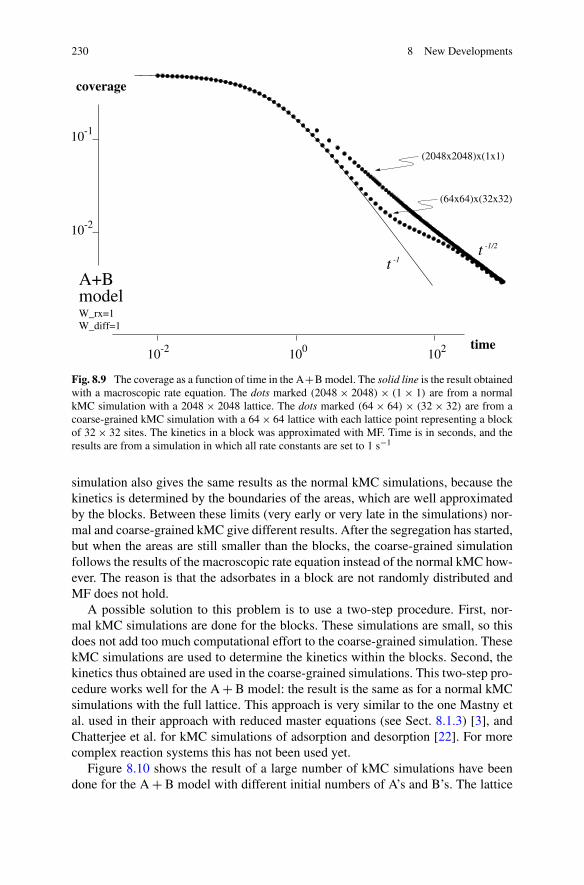
230 8 New Developments

Fig. 8.9 The coverage as a function of time in the A+B model. The solid line is the result obtainedwith a macroscopic rate equation. The dots marked (2048 × 2048) × (1 × 1) are from a normalkMC simulation with a 2048 × 2048 lattice. The dots marked (64 × 64) × (32 × 32) are from acoarse-grained kMC simulation with a 64 × 64 lattice with each lattice point representing a blockof 32 × 32 sites. The kinetics in a block was approximated with MF. Time is in seconds, and theresults are from a simulation in which all rate constants are set to 1 s−1

simulation also gives the same results as the normal kMC simulations, because thekinetics is determined by the boundaries of the areas, which are well approximatedby the blocks. Between these limits (very early or very late in the simulations) nor-mal and coarse-grained kMC give different results. After the segregation has started,but when the areas are still smaller than the blocks, the coarse-grained simulationfollows the results of the macroscopic rate equation instead of the normal kMC how-ever. The reason is that the adsorbates in a block are not randomly distributed andMF does not hold.

A possible solution to this problem is to use a two-step procedure. First, nor-mal kMC simulations are done for the blocks. These simulations are small, so thisdoes not add too much computational effort to the coarse-grained simulation. ThesekMC simulations are used to determine the kinetics within the blocks. Second, thekinetics thus obtained are used in the coarse-grained simulations. This two-step pro-cedure works well for the A + B model: the result is the same as for a normal kMCsimulations with the full lattice. This approach is very similar to the one Mastny etal. used in their approach with reduced master equations (see Sect. 8.1.3) [3], andChatterjee et al. for kMC simulations of adsorption and desorption [22]. For morecomplex reaction systems this has not been used yet.

Figure 8.10 shows the result of a large number of kMC simulations have beendone for the A + B model with different initial numbers of A’s and B’s. The lattice

8.3 Embedding kMC in Larger Simulations 231

Fig. 8.10 Correlation FAB in the occupation of neighboring sites for the A + B model. The figureshows the probability that one site of a pair of neighboring sites is occupied by an A and the otherby a B. This correlation is related via WrxθAθBFAB to the rate of the reaction, where θX is thecoverage of X and Wrx is the rate constant of the reaction. The correlation was determined fromsimulations in which all rate constants were set to 1 s−1

size was 128 × 128. These simulations were used to construct a table with the rateof the A + B reaction for any number of A’s and B’s in a 32 × 32 block. This infor-mation was then used in the coarse-grained kMC simulation. This approach is noteasy to use for more complicated systems. The A + B model has only two reactingspecies, so the table is only two-dimensional and therefore small. Moreover, it wasalso possible to do kMC simulations for the blocks with any possible combinationof numbers of A’s and B’s.

For more complicated systems it may well be necessary to only study those cov-erages that are really relevant. It is also necessary to have another representation ofthe rates as a function of the coverages. Such a representation must be flexible sothat it can incorporate incomplete and noisy data of kMC simulations. It must alsobe able to inter- and extrapolate this data to be used in coarse-graining kMC simu-lations. Neural networks might be useful, but this is very much unexplored territory[29, 30].

8.3 Embedding kMC in Larger Simulations

The kMC simulations that we have discussed focus on the processes taking placeon the surface of a catalyst. In a real catalytic system there are also other processes:in particular, processes dealing with transfer of matter and heat. It is quite possiblethat they affect the performance of a catalyst as much as the surface processes.Some studies have been done to extend the kMC simulations to include these otherprocesses.

232 8 New Developments

Fig. 8.11 A lattice-gas model of the surface of a growing copper crystal coupled to a continuummodel representing the liquid [31–35]. The bottom part shows a two-dimensional cross section of athree-dimensional lattice. The black squares represent the copper atoms. The isolated copper atomsdepict atoms still in solution. The arrows indicate hops that model the diffusion of these atoms.The flux of the atoms through the interface between the lattice gas and the continuum model canbe computed from the difference in frequency of upward and downward hops. The top part showsthe continuum model that specifies the concentration of the copper atoms in solution as a functionof distance to the surface. The flux through the interface can be computed in this model from thegradient of the concentration. Both fluxes should be equal

The main focus has been on the mass transport from the liquid or gas phase to thesurface. This has received most attention not in catalysis, but in crystal growth. In aseries of papers from the University of Illinois the electrodeposition of copper wasinvestigated [31–35]. The diffusion of the copper in the liquid was modeled witha continuum diffusion equation. This is a typical approach in modeling the systemexcept for the surface processes. The diffusion model was one-dimensional: only thedirection perpendicular to the surface was modeled and the concentration of copperwas assumed to be independent on the other directions. The diffusion equation wascoupled to a three-dimensional kMC simulation. The third dimension was used inthe kMC simulation to allow for the growth of the crystal.

A major concern in simulations where kMC is combined with a continuum modelis the coupling between the methods. For the copper deposition this was done asfollows (see Fig. 8.11). The bottom part of the third dimension of the lattice in thekMC simulation was used for the growing copper crystal, but the top part was usedto model the part of the liquid in contact with the surface. The diffusion of the copperin that part of the liquid was modeled as hops on the three-dimensional lattice. Thecoupling was accomplished by equating the flux of the copper in the liquid throughthe interface between the continuum part and the kMC lattice. In the continuum partthis flux can be derived from the gradient of the concentration perpendicular to the

8.3 Embedding kMC in Larger Simulations 233

surface. In the lattice part this flux can be computed by averaging over the numberof hops perpendicular to the surface.

Besides mass transport, heat transfer can also be an issue. This was investigatedfor pure heat transfer and a model of desorption by Castonguay and Wang [36]. Twoapproaches were tested. The first incorporated heat into the kMC simulations bymodeling it as so-called thermal bits that could be exchanged between lattice points.The second used a Poisson heat equation that was solved between occurrences ofregular processes. Both approaches were shown to give the same accurate results,but the approach with the Poisson heat equation was faster.

Matera and Reuter took this approach to a new level by including both mass andheat transport [37, 38]. These were modeled by the transient Navier–Stokes equationand conservation of energy and atomic species. They applied their method to a ab-initio model of CO oxidation on RuO2(110). This process had been studied beforeand a comparison between the simulations with and without modeling the massand heat transfer showed substantial differences [39, 40]. The surface kinetics wassometimes hidden in the overall reactivity by transport limitations, and the overallkinetics became more complicated because of various steady states that arose solelyfrom the coupling between the gas transport and surface processes.

The approaches described above all modeled only a relatively small patch of acatalyst’s surface compared to what is found in a reactor. A much more ambitiousapproach was developed by Majumder and Broadbelt [41]. They modeled a wholeflow reactor. (Actually, they modeled only a pore in the support with the catalystdeposited on the inner surface of the pore. The model however can just as well beused for a whole flow reactor. The main difference is the size of the system.) Thisreactor was envisioned as a pipe (see Fig. 8.12). The flow was described by

u∂Ci

∂z= Di

∂2Ci

∂y2(8.51)

with Ci the concentration of component i, Di its diffusion constant, u the localvelocity of the fluid phase, z the coordinate along the pipe, and y the coordinateperpendicular to the surface. Boundary conditions were Ci = C

(0)i for y > 0 and

z = 0 with C(0)i a constant, ∂Ci/∂y = 0 at the center of the pipe, and

Di

∂Ci

∂y= R

(ads)i − R

(des)i (8.52)

with R(ads)i the adsorption rate and R

(des)i the desorption rate of component i. This

last boundary condition couples the kMC simulation to the continuum model for theliquid.

In a flow reactor the processes on the catalyst change the concentrations in theliquid. This however takes place on a much larger length scale than can be modeledby a single kMC simulation. The reactor was therefore spatially discretized in agrid which was used the solve the continuum model. At the boundary where thecatalyst’s surface was found, the last boundary condition (8.52) was handled in oneof two ways. For some lattice points, periodically spaced, a kMC simulation wasdone to determine the adsorption and desorption rates. For the other grid points an

234 8 New Developments

Fig. 8.12 Modeling a flow reactor [41]. The reactor is modeled as a pipe as shown in the top-left.The reactants stream in from the left. The black strips depict the catalyst. The middle shows anenlargement of part of the reactor including same of the catalyst, and the lattice that is used tosolve the continuum equation for the flow. The points at the bottom of the lattice represent thecatalyst. The closed spheres indicate the lattice points that are coupled to a kMC simulations shownat the bottom. The reactivity of the catalyst at the open spheres are derived from interpolating kMCresults

interpolation scheme was used based on the kMC results of nearest lattice points forwhich simulations were done.

The approach was used to study two simple models. The first had adsorption ofA’s on a single site, conversion of the A’s into B’s, and then desorption of B’s. Thismodel was mainly used to make sure that the whole approach gave correct results,as it could also be solved analytically. The other model consisted of adsorption ofA’s and B’s, which together reacted to form C’s which immediately desorbed. Thismodel was used to highlight the difference with the conventional approach with rateequations.

8.4 Off-lattice kMC

Although lattice-gas models are very versatile, there are situations in which it issimply too difficult or cumbersome to model a system with a lattice. Sometimes itis possible to extend the lattice-gas concept while retaining its advantages. For ex-ample, Bos et al. have used multiple lattices to study massive phase transformationsmetals of fcc to bcc [42, 43]. The two lattices (fcc and bcc) cannot be modeled asone lattice that includes all the fcc and bcc sites. So the atoms are allowed to choosebetween the sites of an fcc and of a bcc lattice. In addition some random sites areincluded to make the transition from one to another lattice easier. These sites are

8.4 Off-lattice kMC 235

dynamically added and removed at positions where they prove to be most needed[43]. This approach has still all the advantages of a model with a single lattice, butit is more flexible. We will look here however at not using a lattice at all.

In the derivation of the master equation

dPα

dt=∑

β

[WαβPβ − WβαPα] (8.53)

the subscripts α and β refer to catchment regions or basins of attraction of thecorresponding minimum of the potential-energy surface (PES) of a system (seeSect. 2.2.2) [44]. This means that it is possible to do kMC simulations in whichthe processes are hops on the PES from on basin of attraction of the PES to a neigh-boring one. This can in principle be done for any PES, which would extend theapplicability of kMC compared to its use in combination with lattice-gas modelsenormously. Viewed like this kMC is competitive with a number of methods basedon Molecular Dynamics for simulating atomic systems over long time scales: seethe reviews of Henkelman et al. and Voter et al. [45, 46].

The way kMC works for hopping on a PES is as follows. Suppose that at a certaintime tn the system is near minimum αn of the PES. Then a list of hops αn → β needto be made, with β a neighboring minimum: i.e., a minimum that can be reachedfrom the current one along a continuous curve via a single saddle point of the PES.This means determining all saddle points or transition states of the PES surroundingthe minimum αn. The rate constant Wβαn needs to be computed for each transitionstate that is found. The transition to another minimum αn+1 is then made with aprobability proportional to Wαn+1αn and time is advanced to

tn+1 = tn − ln r∑β Wβαn

(8.54)

with r a uniform deviate on the unit interval. Alternatively, instead of the VSSMalgorithm described here, one of the other algorithms of Chap. 3 can be used just aswell.

The important difference with lattice-gas kMC is that the processes are no longerknown before a kMC simulation is started, but they have to be determined on-the-fly.This makes this general kMC method much more costly. Determining a transitionstate for a process is costly in itself, but the task here is especially daunting becausein principle all transition states around a minimum have to be determined. Never-theless, this approach has been used, even in combination with Density-FunctionalTheory calculations, in the pioneering work by Henkelman and Jónsson [47, 48].They applied it to diffusion of clusters of Al atoms on an Al surface. This workshowed a very important advantage of the method. Because the processes are notprecomputed, surprising processes may show up and may turn out to be highly rel-evant. In Henkelman and Jónsson’s work diffusion of the clusters took place withconcerted motions that included the atoms of the surface as well. Early applica-tion were also done on the formation of defects during crystallization [49], and thesegregation of atoms [50].

236 8 New Developments

Although there are methods that can insure finding all transition states around aminimum [51–53], these are extremely costly. Sometimes it is possible, similarlyto lattice-gas kMC, to say in advance what the processes are. For example, in astudy on diffusion in binary alloys a vacancy could move in only twelve possible di-rections [54]. Consequently, the transition states were at least approximately knownand needed only to be refined. The same approach could be used in a study on H dif-fusion in iron [55], and in a similar study of vacancy diffusion in crystalline silicon alist could be made during a simulation with topological characteristics of diffusionmechanisms to facilitate finding transition states [56]. In general, however, this isnot possible. In their seminal work Henkelman and Jónsson started each search fora new transition state with a random displacement of all atoms and then did 25 to 50searches from each minimum [47]. In a later study more selective initial displace-ments were tested [57]. These studies naturally lead to the question how one knowsthat all transition states have been found.

This question was given a statistical answer by Xu and Henkelman [57]. Theyargued that if there are T transition states, one has already found F different ones,and each transition state has the same probability of being found, then the proba-bility of having found all transition states equals F/T . This equation is not usefulas one does not know T . However, if one finds only one new transition state per S

searches, then F/T = 1 − 1/S. So the latter expression can be used as a criterion tostop looking for new transition states. One simply requires 1 − 1/S to be larger thansome preset value.

Some Bayesian statistics can put this criterion on a firmer footing. The proba-bility that the next transition state search, number n, will find a new transition state(Xn = 1) is given by

P(Xn = 1|Fn−1T ) = T − Fn−1

T, (8.55)

and the probability of finding one that has been found before (Xn = 0) equals

P(Xn = 0|Fn−1T ) = Fn−1

T. (8.56)

Here Fn−1 is the number of transition states found after n − 1 searches. FromBayes’s theorem

P(Xn|Fn−1T )P (T |Fn−1) = P(XnT |Fn−1) = P(T |Fn−1Xn)P (Xn|Fn−1) (8.57)

we get

P(T |Fn−1Xn) ∝ P(Xn|Fn−1T )P (T |Fn−1). (8.58)

So if we have the probabilities P(T |Fn−1) that there are T transition states, thena new transition state search will change these probabilities. If it leads to a newtransition state, then the probabilities should be multiplied by (T − Fn−1)/T , if notby Fn−1/T . (The probabilities of course also need to be normalized.) Subsequenttransition state searches will make P(T |Fn) sharper peaked. One should stop if themaximum P(T |Fn) becomes larger than some preset value.

8.4 Off-lattice kMC 237

Initially we have F0 = 0 and let’s assume P(T |F0) = 1/M with M a numberthat is larger than the number of transition states. Suppose we do S searches. Wecan then write

P(T |FS) = A(T ,FS)

T S(8.59)

From Eqs. (8.55) to (8.58) we can see that A(T ,FS) is a product of factors T − Fm,Fm, and a normalization constant. The Fm’s here are the number of transition statesfound so far during the searches. Because we started with F0 = 0 these factors yieldT (T − 1)(T − 2) . . . (T − FS + 1). There is one factor for every time that a newtransition state was found. For searches that did not yield a new transition state weget some factor Fm. Because such a factor does not affect the T -dependence ofP(T |FS) we can include these factors in the normalization constant. So we have

P(T |FS) ={

N T !(T −FS)!T S , if T ≥ FS ,

0, if T < FS ,(8.60)

with N a normalization constant.The probability P(T |FS) has a single maximum. If we want to know if we have

found all transition states, then we want that maximum to be at T = FS . From

P(T = FS + 1|FS)

P (T = FS |FS)= FS

S

(FS + 1)S−1< 1 (8.61)

we then get

S >ln(FS + 1)

ln(FS + 1) − lnFS

. (8.62)

This is however only a lower bound for the number of searches that we need to do.It insures that the number of transition states that we have found is the most likelynumber of transition states, but in general we want the probability that we havefound all transition states to be higher: i.e., we will require P(T = FS |FS) > Pfoundwith Pfound to be some number close to 1. Figure 8.13 shows how many searchesone needs to do to achieve such higher probabilities. We see that the number ofsearches is a factor of two to three higher than the lower bound depending on theactual number of transition states and how certain one wants to be that one has foundall transition states. We also see that when there are more transition states that wealso need to do more searches per transition state.

An even better criterion can be given if one realizes that one does not really needto known all transition states. One only needs to know that one that correspondsto the process that will take place first. Instead of the VSSM expression (8.54) onecan also use FRM and compute a time for each transition state (see Sect. 3.5). Thenthe problem becomes finding the transition state with the smallest value for thattime: i.e., the one corresponding the first process to occur. We will not determineall transition states to compare all times, but we will give a statistical criterion thatgives us a probability that we have found the first process to take place.

We define two new stochasts. Stochast Yn = 1 if at transition state search n wefind a transition state of an earlier process than any we have found so far, and Yn = 0

238 8 New Developments

Fig. 8.13 The number of transition states searches per transition state that are needed to achievea probability of 0.99, 0.95, or 0.9 (markers from top to bottom) that all transition states have beenfound as a function of the actual number of transition states. The curve indicates the situation thatthe number of transition states that have been found is the most likely number of transition states

if that is not the case. Stochast Rn is the rank number of the transition state that hasbeen found after n searches corresponding to the earliest process: i.e., the first ofall processes has rank Rn = 1, the second Rn = 2, et cetera. Of course, we do notknow the value of Rn, but we can make some statistical inferences from finding newtransition states corresponding to earlier processes.

We have

P(XnYn|T Fn−1Rn−1) =

⎧⎪⎨

⎪⎩

Rn−1−1T

, if Xn = Yn = 1,Fn−1

T, if Xn = Yn = 0,

T −(Rn−1−1)−Fn−1T

, if Xn = 1 and Yn = 0.

(8.63)

Note that Xn = 0 and Yn = 1 is not possible: if we find a transition state of an earlierprocess it must also be a new transition state. Bayes’s theorem then gives

P(T Rn−1|Fn−1XnYn) ∝ P(XnYn|T Fn−1Rn−1)P (T Rn−1|Fn−1). (8.64)

This is however not quite what we want. We do not want the probabilities for Rn−1but for Rn. If Xn = 0 or Yn = 0, then there is no new transition state of an earlierprocess, and P(T Rn|Fn−1XnYn) = P(T Rn−1|Fn−1XnYn). If Yn = 1, and henceXn = 1, then the new transition state corresponds to an earlier process: i.e., it hasa rank number smaller than Rn−1. Of course, we do not know the value of Rn, butwe can use the same assumption as before that all transition states with Rn < Rn−1are equally likely. This means that the probabilities P(T Rn−1|Fn−1XnYn) shouldbe equally divided into the probabilities P(T Rn|Fn−1XnYn) with Rn < Rn−1, or

P(T Rn|Fn−1XnYn) =T∑

Rn−1=Rn+1

1

Rn−1 − 1P(T Rn−1|Fn−1XnYn). (8.65)

8.4 Off-lattice kMC 239

Fig. 8.14 The number of transition states searches per transition state that are needed to achieve aprobability of 0.99, 0.95, or 0.9 (markers from top to bottom) that the first process to occur has beenfound as a function of the actual number of transition states (see Fig. 8.13). The curve indicates thesituation that the number of transition states that have actually been found is also the most likelynumber of transition states

This expression will give a strong concentration of probabilities for lower values ofRn. This is advantageous, because we really want to know the probability that wehave found the first process of all: i.e., we want P(T ,Rn = 1|Fn−1XnYn).

We start as before with assuming that P(T |F0) =∑TR0=1 P(T R0|F0) = c/M

with c a normalization constant. We also assume that all values for R0 are equallylikely, so P(T R0|F0) = c/MT . Figure 8.14 shows the number of transition searchthat needs to be done to find the first process with different probabilities. We noticetwo differences with respect to trying to find all transition states. First the number ofsearches is significant smaller. The curve in Fig. 8.14 is the same one as in Fig. 8.13and indicates a lower bound for the number of searches to find all transition states.If there are many transition states we need not even do so many searches if we onlywant to find the first process to occur. This makes sense, because it is of courseharder to find all transition states than to find one particular transition state. Thesecond differences is that the number of searches per transition state does not in-crease with the actual number of transition states, but seems to be constant for manytransition states and even decreases if there are few transition states. This is a morefavorable behavior than was seen for finding all transition states.

Xu and Henkelman also looked at the case when not all transition states areequally likely to be found, which is more realistic for the methods that are generallyused in the transition state searches. They have a higher probability of finding low-energy transition states.

Some other techniques have been used to deal with the problem of finding transi-tion states. An obvious one is to save transition states that have already been found[57, 58]. For example, when a process has just occurred, the transition state for thereverse process is then of course known. By constructing the graph of minima that

240 8 New Developments

are connected via transition states, no transition state needs to be done for minimathat are visited again. In fact, it might even be possible to use one of the methodsin Sect. 8.1.4 and use multistep processes so that the simulation only goes to newminima. For example, a superbasin approach was used by Xu and Henkelman todeal with fast processes with low-energy transition states [57].

A more sophisticated approach attempts to use the fact that different transitionstates may resemble each other [57, 59]. Suppose that we are at a certain mini-mum and that two processes are possible that affect different parts of the systemthat are far apart. Suppose that one of these processes takes place. The system thengets to another minimum with a new set of transition states. However, the processthat did not take place in the original minimum is still possible, but correspondsstrictly speaking to another transition state. It should be relatively easy to determinethis new transition state using the information of the transition states of the origi-nal minimum. This has been called recycling transition states. It is very similar towhat is done in the algorithms of lattice-gas kMC when lists of processes are notrecomputed but only updated.

There have been few studies yet using off-lattice kMC so far. It remains to beseen how big the problem is of finding transition states on-the-fly. Increasing thesystem size seems to increase the number of transition states exponentially [60].Recycling may change this unfavorable scaling just as it does for lattice-gas kMC.Much more work needs definitely to be done.

For some systems off-lattice kMC needs not be so much more time consumingthan lattice-gas kMC. For reactions in solvents it is possible to use lattice-gas mod-els [61–65]. The drawback is that a lot of computer time is spent on diffusion ofparticles that need to find each other first before they can react. It has recently beenshown that this need not be necessary [66]. It can be assumed that diffusion in thesolvent is a Brownian motion. This can be treated analytically, which leads to effec-tive rate constants that depend on the distance between the reacting particles whenthey are formed and their diffusion constants. Moreover, there is also a factor that isan intrinsic rate constant, which can be computed before doing the kMC simulation.This makes the simulation more efficient than simulations in which rate constantsare computed on-the-fly [67, 68].

References

1. A. Chatterjee, F. Voter, J. Chem. Phys. 132, 194101 (2010)2. S.V. Nedea, A.P.J. Jansen, J.J. Lukkien, P.A.J. Hilbers, Phys. Rev. E 65, 066701 (2002)3. E.A. Mastny, E.L. Haseltine, J.B. Rawlings, J. Chem. Phys. 125, 194715 (2006)4. D.R. Mason, R.E. Rudd, A.P. Sutton, Comput. Phys. Commun. 160, 140 (2004)5. R.E. Rudd, D.R. Mason, A.P. Sutton, Prog. Mater. Sci. 52, 319 (2007)6. N.G. van Kampen, Stochastic Processes in Physics and Chemistry (North-Holland, Amster-

dam, 1981)7. S.X. Sun, Phys. Rev. Lett. 96, 210602 (2006)8. S.A. Trygubenko, D.J. Wales, Graph transformation method for calculating waiting times in

Markov Chains. http://arXiv.org/abs/cond-mat/0603830 (2006)

References 241

9. L. Kantorovich, Phys. Rev. B 75, 064305 (2007)10. T. Oppelstrup, V.V. Bulatov, G.H. Gilmer, M.H. Kalos, B. Sadigh, Phys. Rev. Lett. 97, 230602

(2006)11. T. Oppelstrup, V.V. Bulatov, A. Donev, M.H. Kalos, G.H. Gilmer, B. Sadigh, Phys. Rev. E 80,

066701 (2009)12. A. Donev, V.V. Bulatov, T. Oppelstrup, C.H. Gilmer, B. Sadigh, M.H. Kalos, J. Comput. Phys.

229, 3214 (2010)13. D.T. Gillespie, J. Chem. Phys. 115, 1716 (2001)14. D.T. Gillespie, L.R. Petzold, J. Chem. Phys. 119, 8229 (2003)15. Y. Cao, L. Petzold, M. Rathinam, D.T. Gillespie, J. Chem. Phys. 121, 12169 (2004)16. D.G. Vlachos, Phys. Rev. E 78, 046713 (2008)17. M.A. Katsoulakis, A.J. Majda, D.G. Vlachos, Proc. Natl. Acad. Sci. USA 100, 782 (2003)18. M.A. Katsoulakis, A.J. Majda, D.G. Vlachos, J. Comput. Phys. 186, 250 (2003)19. M.A. Katsoulakis, D.G. Vlachos, J. Chem. Phys. 119, 9412 (2003)20. A. Chatterjee, D.G. Vlachos, J. Chem. Phys. 121, 11420 (2004)21. M.A. Snyder, A. Chatterjee, D.G. Vlachos, Comput. Chem. Eng. 29, 701 (2005)22. A. Chatterjee, D.G. Vlachos, J. Chem. Phys. 124, 064110 (2006)23. A. Chatterjee, D.G. Vlachos, J. Comput. Phys. 211, 596 (2006)24. A. Chatterjee, D.G. Vlachos, J. Comput.-Aided Mater. Des. 14, 253 (2007)25. S.D. Collins, A. Chatterjee, D.G. Vlachos, J. Chem. Phys. 129, 184101 (2008)26. J. Dai, D. Seider, T. Sinno, J. Chem. Phys. 128, 194705 (2008)27. S. Are, M.A. Katsoulakis, A. Szepessy, Chin. Ann. Math., Ser. B 30, 653 (2009)28. S. Redner, in Nonequilibrium Statistical Mechanics in One Dimension, ed. by V. Privman

(Cambridge University Press, Cambridge, 1996), pp. 3–2729. K. Gurney, An Introduction to Neural Networks (University College London Press, London,

1997)30. J. Hertz, A. Krogh, R.G. Palmer, Introduction to the Theory of Neural Computation (Addison-

Wesley, Redwood City, 1991)31. T.J. Pricer, M.J. Kushner, R.C. Alkire, J. Electrochem. Soc. 149, C396 (2002)32. T.J. Pricer, M.J. Kushner, R.C. Alkire, J. Electrochem. Soc. 149, C406 (2002)33. T.O. Drews, E.G. Webb, D.L. Ma, J. Alameda, R.D. Braatz, R.C. Alkire, AIChE J. 50, 226

(2004)34. E. Rusli, T.O. Drews, R.D. Braatz, Chem. Eng. Sci. 59, 5607 (2004)35. Z. Zheng, R.M. Stephens, R.D. Braatz, R.C. Alkire, L.R. Petzold, J. Comput. Phys. 227, 5184

(2008)36. T.C. Castonguay, F. Wang, J. Chem. Phys. 128, 124706 (2008)37. S. Matera, K. Reuter, Catal. Lett. 133, 156 (2009)38. S. Matera, K. Reuter, Phys. Rev. B 82, 085446 (2010)39. K. Reuter, M. Scheffler, Phys. Rev. B 68, 045407 (2003)40. K. Reuter, M. Scheffler, Phys. Rev. B 73, 045433 (2006)41. D. Majumder, L.J. Broadbelt, AIChE J. 52, 4214 (2006)42. C. Bos, F. Sommer, E.J. Mittemeijer, Acta Mater. 52, 3545 (2004)43. C. Bos, F. Sommer, E.J. Mittemeijer, Acta Mater. 53, 5333 (2004)44. P.G. Mezey, Potential Energy Hypersurfaces (Elsevier, Amsterdam, 1987)45. G. Henkelman, G. Jóhannesson, H. Jónsson, in Progress in Theoretical Chemistry and

Physics, ed. by S.D. Schwarts (Kluwer Academic, London, 2000)46. A.F. Voter, F. Montalenti, T.C. Germann, Annu. Rev. Mater. Res. 32, 321 (2002)47. G. Henkelman, H. Jónsson, J. Chem. Phys. 115, 9657 (2001)48. G. Henkelman, H. Jónsson, Phys. Rev. Lett. 90, 116101 (2003)49. F. Much, M. Ahr, M. Biehl, W. Kinzel, Comput. Phys. Commun. 147, 226 (2002)50. T.F. Middleton, D.J. Wales, J. Chem. Phys. 120, 8134 (2004)51. K.M. Westerberg, C.A. Floudas, J. Chem. Phys. 110, 9259 (1999)52. Y. Lin, M.A. Stadtherr, J. Chem. Phys. 121, 10159 (2004)53. Y. Lin, M.A. Stadtherr, J. Comput. Chem. 26, 1413 (2005)

242 8 New Developments

54. E.A. Bleda, X. Gao, M.S. Daw, Comput. Mater. Sci. 43, 608 (2008)55. A. Ramasubramaniam, M. Itakura, M. Ortiz, E.A. Carter, J. Mater. Res. 23, 2757 (2008)56. F. El-Mellouhi, N. Mousseau, L.J. Lewis, The kinetic activation-relaxation technique: A pow-

erful off-lattice on-the-fly kinetic Monte Carlo algorithm. http://arXiv.org/abs/0805.2158v1(2008)

57. L. Xu, G. Henkelman, J. Chem. Phys. 129, 114104 (2008)58. D.R. Mason, T.S. Hudson, A.P. Sutton, Comput. Phys. Commun. 165, 37 (2005)59. A. Kara, O. Trushin, H. Yildirim, T.S. Rahman, J. Phys., Condens. Matter 21, 084213 (2009)60. R.A. Olsen, G.J. Kroes, G. Henkelman, A. Arnaldsson, H. Jónsson, J. Chem. Phys. 121, 9776

(2004)61. M. Jorge, S.M. Auerbach, P.A. Monson, J. Am. Chem. Soc. 127, 14388 (2005)62. M.H. Ford, S.M. Auerbach, P.A. Monson, J. Chem. Phys. 126, 144701 (2007)63. L. Jin, S.M. Auerbach, P.A. Monson, J. Phys. Chem. C 114, 14393 (2010)64. A. Malani, S.M. Auerbach, P.A. Monson, J. Phys. Chem. Lett. 1, 3219 (2010)65. A. Malani, S.M. Auerbach, P.A. Monson, J. Phys. Chem. C 115, 15988 (2011)66. X.Q. Zhang, A.P.J. Jansen, Phys. Rev. E 82, 046704 (2010)67. X.Q. Zhang, T.T. Trinh, R.A. van Santen, A.P.J. Jansen, J. Am. Chem. Soc. 133, 6613 (2011)68. X.Q. Zhang, T.T. Trinh, R.A. van Santen, A.P.J. Jansen, J. Phys. Chem. C 115, 9561 (2011)

Glossary

absorbing state A state of a master equation from which there is no transition pos-sible to another state (Sect. 2.2.1). If the master equation describes the evolutionof an adlayer, then a state is a configuration and an absorbing state corresponds topoisoning.

activation barrier When one or more molecules react the potential energy in-creases from a minimum value, reaches a maximum, and then decreases to anotherminimum value. The activation barrier is the difference between the maximum andthe initial minimum value. It is an energy threshold that needs to be overcomefor a reaction to occur (Sect. 4.2). Sometimes zero-point energy is added to theinitial minimum and the maximum to get a zero-point corrected activation barrier(Sect. 4.3.2). The concept is closely related to the activation energy.

activation energy A parameter in the Arrhenius expression for rate constants thatdescribes how a rate constant changes with temperature. The activation energy isclosely related to the activation barrier, as the latter is the dominant contribution tothe activation energy, but they are not quite the same (Sect. 4.2.2).

adlayer The layer on top of the substrate where the adsorbates are found.adsorption Process in which an atom or a molecule from the gas phase or from a

solution attaches itself to a surface. It is the reverse of a desorption.adsorption site A preferred position for an atom, a molecule, or a molecular frag-

ment on a surface. This position corresponds to a minimum of the potential-energysurface (Sect. 2.1).

Arrhenius form An expression that describes the rate constant as depending ex-ponentially on the reciprocal temperature. It has two parameters: the activationenergy and the prefactor (Sect. 4.2.2).

bookkeeping site A lattice point in a lattice-gas model that does not correspond toan adsorption site, but that is used to store information that simplifies running asimulation (Sect. 5.5.4).

cluster expansion A mathematical expression that can be used to express the lat-eral interactions in an adlayer. It is a sum of terms that correspond to interactionsbetween adsorbates and substrate, between pairs of adsorbates, between triplets ofadsorbates, between quadruplets of adsorbates, et cetera (Sect. 4.5.1).

A.P.J. Jansen, An Introduction to Kinetic Monte Carlo Simulations of SurfaceReactions, Lecture Notes in Physics 856,DOI 10.1007/978-3-642-29488-4, © Springer-Verlag Berlin Heidelberg 2012

243

244 Glossary

coarse-graining A technique in which an atomic scale description is replaced byone with a longer length scale. In kinetic Monte Carlo coarse-graining is usedwhen the (catchment regions of the) minima of a potential-energy surface areused instead of the precise values of the coordinates and velocities of the atoms(Sect. 2.2.2), and when lattice is used with each lattice point corresponding to ablock of sites instead of a single site (Sect. 8.2).

configuration The lattice points in lattice-gas models that are used in kinetic MonteCarlo all have a label. A particular assignment of values to all the labels in a lattice-gas model is called a configuration. If each lattice point corresponds to an adsorp-tion site (as is often the case), then a configuration is also a particular way todistribute adsorbates over the adsorption sites (Sect. 2.1.3).

configuration space If we take all coordinates of all Natom atoms of a molecularsystem and put them together to form one vector with 3Natom components, thenthe vector space formed by such vectors is the configuration space of the molecularsystem. Potential-energy surfaces are defined on the configuration space, and thespace is also important in statistical physics.

coordination number The number of neighbors of a adsorption site or an atom(Sects. 4.6.6, 4.6.7, and 6.7).

coverage The density of the adsorbates. It is most often defined as the numberof adsorbates per number of unit cell of the substrate, but also as the number ofadsorbates per number of adsorption sites or per unit area.

defect A change in structure that destroys periodicity or translational symmetry(Sect. 5.5.3).

desorption A process in which an atom or a molecule detaches itself from a surfaceand goes into the gas phase or a solution. It is the reverse of an adsorption.

diffusion A random motion of an atom, a molecule, or a molecular fragment that isa consequence of collisions with other particles or the interaction with the thermalmotion of other particles. It corresponds to random hops from one adsorption siteto a neighboring one in a lattice-gas model.

diffusion coefficient A parameter describing the rate of diffusion. Apart from aconstant is a proportionality factor between the square of a displacement and time(Sect. 4.6.5).

disabled process A process that is no longer possible because of changes in thesystem by other processes (Sects. 3.2.3 and 3.3.2). It is also called a null event.

dissociation A process in which a molecule is split into two or more parts. It is thereverse of a formation.

dividing surface In the derivation of the master equation phase space is partitionedinto regions that correspond to the minima of the potential-energy surface or con-figurations of an adlayer. The boundaries separating the regions in phase space arecalled dividing surfaces (see Sect. 2.2.2). The term originates from a derivation ofVariational Transition-State Theory in which phase space is split into a part corre-sponding to reactants and a part corresponding to products separated by a dividingsurface.

dynamic correction factor Sometimes a process occurs but it is immediately fol-lowed by the reverse of the process. A calculation of the rate constants for the

Glossary 245

processes will give higher values when we regard forward and reverse processactually having taken place, than when we assume that effectively nothing hashappened. The latter is regarded the correct approach. The factor that corrects foroverestimated rate constants that are obtained from the former approach is calledthe dynamic correction factor (Sect. 4.4.3).

Eley–Rideal reaction Chemical reaction with reactants both on a surface and inthe gas phase or in a solution (Sect. 4.4.4).

enabled process A process that is possible (Sect. 3.2.3). The term is mainly usedto distinguish it from a disabled process.

event The actual occurrence of a process (Sects. 2.1 and 3.2.2).event list A list of all possible processes that can occur at a certain moment in a

simulation (Sect. 3.2.3). This list includes besides the processes that actual willoccur (i.e., the events) also other processes. These other processes never occur,because, before they can occur, the system changes in such a way that they are nolonger possible. We prefer the term “list of all processes” in this book. This is lesssuccinct but also less confusing.

First Reaction Method An algorithm of kinetic Monte Carlo in which a time iscomputed for each possible process. The process that actually takes place is thenthe one with the smallest value for the time (Sect. 3.5).

flicker process A process that is very rapidly followed by its reverse process(Sect. 8.1.4).

floppy molecule A floppy molecule is a molecule with a potential-energy surfacethat has many minima that are separated by barriers that can easily overcome bythermal excitation or tunneling.

fluctuation Random variations of some property around an average value(Sect. 5.2).

formation A process in which atoms or molecular fragments get together to forma molecule. It is the reverse of a dissociation.

immediate process A process with an infinitely large rate constant (Sect. 5.3). Thetime in a simulation does not change when an immediate process takes place. Im-mediate processes are mainly used for changes in the configuration that are toocomplicated to be described by a single process. They are often used together withbookkeeping sites.

interaction model A particular way to describe the lateral interactions between ad-sorbates (Sect. 4.5.1).

inverted list A list that specifies the processes that are possible for each adsorbate(Sect. 3.3.2). This list can be regarded as the inverse (hence its name) of the eventlist.

label Each lattice point in a lattice-gas model has a label. This label specifies thestatus of the lattice point (Sect. 2.1.3). We represent labels in this book by stringsbecause of their flexibility (Sect. 5.3). The most common use of labels is to indicatethe occupation of adsorption sites, but they have many other uses in particular incombination with bookkeeping sites and immediate processes (Chaps. 5 and 6).

Langmuir–Hinshelwood reaction Chemical reaction with all reactants on a sur-face (Sect. 4.4.1).

246 Glossary

lateral interaction Interaction between two or more adsorbates (Sect. 4.5). Lateralinteractions include direct interactions, but also interactions that are a consequenceof adsorbates changing the electronic structure of the substrate or displacing theatoms of the substrate and thereby inducing stress.

lattice A collection of discrete points that is invariant under certain shifts or trans-lations (Sect. 2.1). For a simple lattice the vectors connecting the points can bewritten as a linear combination of basis vectors with integer coefficients. Thesebasis vectors are called primitive vectors. A composite lattice is a collection of twoor more interpenetrating simple lattices with the same primitive vectors.

lattice gas A lattice with a label for each lattice point (Sect. 2.1).long-range order Strong correlation in the structure of a system over a much

longer distance than the range of the interactions in the system (Sects. 7.2and 7.4.1).

macroscopic equation An equation that describes how a statistical average ofsome property changes with time (Sect. 4.6.1). It is also called the phenomeno-logical equation. It is derived from the master equation. The name indicates thatone generally uses it for macroscopic properties, although it also holds for otherproperties. If the property is a coverage, then it is often also called macroscopicrate equation or just rate equation. Note however that the macroscopic equation isexact, whereas a rate equation often implies that a Mean Field Approximation hasbeen used.

Markov chain A sequence of Markov processes.Markov process A process that depends only on the current state of a system and

not on the system’s history (Sect. 2.2.1).master equation A linear equation that describes how the probabilities of various

states of a system change in time (Sect. 2.2.1). The equation conserves the totalprobability of all states. For kinetic Monte Carlo the states are configurations of alattice-gas model.

Mean Field Approximation Name for various similar approximations. For lattice-gas models it assumes a random distribution of the adsorbates over the adsorptionsites.

noise Random variations of some property around an average value (Sect. 5.2).Another term for noise is fluctuation.

null event A process that is no longer possible because of changes in the system byother processes. We prefer the term “disabled process” in this book (Sect. 3.3.2).

occupation A specification of the adsorbate on a site (Sect. 2.1).overfitting A situation in a fitting process where the fit not only describes the un-

derlying data but also the errors in that data (Sect. 4.5.1).oversampling A two-step procedure. In the first step numbers are generated or

items chosen with (transition) probabilities that are too high. In the second stepthere is a correction for the incorrect (transition) probability (Sects. 3.3.1, 3.3.4,and 3.4).

partition function A function of the thermodynamic variables that define a statis-tical ensemble and from which other thermodynamic variables can be calculated(Sect. 4.3).

Glossary 247

phase space If we take all coordinates and all conjugate momenta of all Natomatoms of a molecular system and put them together to form one vector with 6Natomcomponents, then the vector space formed by such vectors is the phase space ofthe molecular system.

phase transition Discontinuity in the properties of a system when external condi-tions are changed (Sect. 7.4).

phenomenological equation An equation that describes how a statistical averageof some property changes with time (Sect. 4.6.1). It is also called the macroscopicequation. It can be derived from the master equation.

poisoning Situation in which no chemical reactions on a surface are possible any-more because the presence of some chemical species prevents the adsorption ofone or more reactants (Sect. 7.4.3).

potential-energy surface A function that gives the potential energy of a molecularsystem as a function of the position of the atoms. If there are Ndof degrees offreedom, then the function can be represented as a surface in a space of dimensionNdof + 1.

pre-exponential factor It is the factor in the Arrhenius form of a rate constant be-sides the exponential factor that describes the temperature dependence of a rateconstant. The rate constant becomes equal to the prefactor at infinitely high tem-perature (Sect. 4.2.2).

prefactor Short for pre-exponential factor.primitive vector A vector of a minimal set of vectors that generate a simple lattice.

The lattice is obtained by taking all linear combination of the primitive vectorswith integer coefficients (Sect. 2.1.1). A primitive vector is also called a primitivetranslation.

process A description of how labels of a lattice-gas model can change or the changeitself. The description consists of a list of lattice points, the labels that are to bechanged, and the labels into which they are changed (Sect. 2.1.3). Processes areoften actual physical processes or chemical reactions. We use in this book alsoprocesses that are only defined to facilitate a simulation and that often use book-keeping sites and labels that do not correspond to adsorbates.

Random Selection Method An algorithm of kinetic Monte Carlo in which it isassumed that all processes have the same rate constant and that each process cantake place anywhere on the surface. Oversampling is then used to correct for thisobviously erroneous assumption (Sect. 3.4).

rate The magnitude of the change of some property with time. Mathematically it isthe first derivative of that property with respect to time. In kinetics the property isgenerally a concentration, a density, or a coverage.

rate constant A proportionality constant between a rate and some other propertyof a system. In kinetics this property is generally of the same type as the propertyof the rate: i.e., we write the rate with which a coverage changes as a rate constanttimes some expression of the same or other coverages. Note that we make a strictdistinction between a rate and a rate constant. There are two kinds of rate constantsin this book. One is found in the master equation and is also called the transitionprobability per unit time (Sect. 2.2). The other kind is found in macroscopic rateequations (Sect. 4.6).

248 Glossary

rate equation An equation that describes how a property changes with time(Sect. 4.6.1). It is also called the macroscopic rate equation and the property isusually a concentration or a coverage (Sect. 4.6).

reaction-diffusion equation An extension of the macroscopic rate equation for thecoverage or concentration in which the coverage or concentration is allowed to varywith position. In addition to the terms in the macroscopic rate equation there is alsoa term for describing diffusion.

short-range order Strong correlation in the structure of a system over a distancecomparable to the range of the interactions in the system (Sect. 7.2).

site Short for adsorption site.sticking coefficient The fraction of the total number of atoms and molecules in the

gas phase or solution that hit a surface and that also adsorb (Sect. 4.4.3).sublattice A lattice can either be simple or composite. A composite lattice consists

of two or more identical simple lattices that are shifted with respect to each other.Such a simple lattice is called a sublattice (Sect. 2.1).

superbasin A collection of catchment regions (or basins of attraction) of minimaof a potential-energy surface. The catchment regions should be neighbors and thesuperbasin is a connected region (Sect. 8.1.2).

supertype A collection of different types of processes that are given the same rateconstant. A supertype is used together with oversampling to correct for the fact thatsome types of processes forming the supertype have a smaller rate constant than isgiven to the supertype (Sect. 3.3.4).

surface reconstruction A structure of a surface that is different from the one that isobtained by cutting a crystal, or the change that leads to that structure (Sects. 5.5.3,7.3, and 7.5).

symmetry breaking Phenomenon where a system changes in such a way that thesymmetry group of the system is reduced to that of a subgroup (Sect. 7.4).

Temperature-Programmed Desorption Experimental technique in which an ad-layer is heated up and the desorption of atoms and molecules is monitored. If dur-ing the experiment there are also reactions on the surface, then one also talks aboutTemperature-Programmed Reaction (Sects. 3.6 and 7.2).

transition matrix A matrix that gives the probabilities with which a systemchanges from one configuration into another (Sect. 8.1.4). The transition matrixis closely related to the matrix of transition probabilities of the master equation.

transition probability This is short for transition probability per unit time. It isa parameter in the master equation (Sect. 2.2.1). Because of the similarity andbecause the term is better known, we mostly use the term “rate constant” insteadof transition probability in this book.

transition state When one or more molecules react their potential energy increasesfrom a minimum value, reaches a maximum, and then decreases to another min-imum value. The structure of the molecule(s) corresponding to the maximum en-ergy is called the transition state (Sect. 4.2).

Transition-State Theory An approximation to calculate rate constants. There aremany assumptions that can be made that all lead to the same expression. In rela-tion to the derivation of the master equation in this book the assumption is thatrecrossings of the dividing surface is ignored (Sects. 4.2 and 4.4.3).

Glossary 249

unit cell A representative part of a periodic system or system with translationalsymmetry. The whole system can be obtained by making copies the unit cell andshifting them over all symmetry translations (Sect. 2.1).

Variable Step Size Method An algorithm of kinetic Monte Carlo in which a singletime is computed for each configuration that is encountered during a simulation andwhere processes are chosen proportional to their rate constants (Sects. 3.2 and 3.3).The method is also often called the n-fold way.

voltammetry Experimental technique in which the potential of an electrode ischanged and the current is measured that is caused by reactions on the electrode’ssurface (Sects. 3.6 and 7.4.2).

zero-point energy The difference in energy between the energy of the minimum ofa potential-energy surface and the ground state energy (Sect. 4.3.2).

Ziff–Gulari–Barshad model A simple model for CO oxidation that has only threeprocesses: adsorption of CO, dissociative adsorption of molecular oxygen, and for-mation and immediate desorption of CO2 (see Sect. 7.4.3).

Index

AAbsorbing state, 24, 202, 216Activation barrier, 11, 75, 78Activation energy, 76, 78

Brønsted–Polanyi relation, 103definition of, 76, 77

Adlayer, 22, 28, 75, 105, 158island, 178ordered, 2, 94, 159, 178, 179, 226structure, 2, 3, 11, 21, 59, 95superstructure, 178

Adsorption, 87–92, 147, 212, 218, 219dissociative, 114, 115, 165, 174modeling, 128, 129, 136, 149, 156, 165,

167–170, 174, 176precursor-mediated, 167–170simple, 108–110, 128, 129, 156, 170, 174,

176sticking coefficient, 89–91

Adsorption site, 14, 126label, 18, 126, 171lattice point, 14, 126modeling, 133–141, 171occupation, 14, 18

AlgorithmFirst Reaction Method, 53parallel, 61–64Random Selection Method, 52rejection-free, 48Variable Step Size Method, 40–50

Arrhenius form, 76, 77

BBookkeeping site, 144, 146, 160, 161

label, 141

CCluster expansion, 94–96

truncation, 95Coarse-graining, 226–231Configuration, 18, 22

initial, 177–179Continuum model, coupling to, 231–234

DDefect, 9, 140Desorption, 86, 87, 89, 92, 122, 156, 169, 170,

212, 218, 219associative, 130, 131, 165modeling, 128–131, 156, 165, 169, 170,

176simple, 106–108, 128, 129, 176

Diffusion, 5, 91, 109–111, 130–132, 141, 148,162, 163, 166–169, 212, 221, 222,226

modeling, 130–132, 141, 148, 162, 163,166–169

Diffusion coefficient, 111, 167Dissociation, 134, 162, 170

modeling, 134, 170Dividing surface, 30Dynamic correction factor, 90

EEvent

event list, 42null event, 48

Event list, 42

FFirst Reaction Method, 53–55, 219, 237

algorithm, 53scaling with system size, 54, 66

A.P.J. Jansen, An Introduction to Kinetic Monte Carlo Simulations of SurfaceReactions, Lecture Notes in Physics 856,DOI 10.1007/978-3-642-29488-4, © Springer-Verlag Berlin Heidelberg 2012

251

252 Index

time-dependent rate constant, with, 56Floppy molecule, 84, 85Fluctuation, 112, 113, 193, 195Formation, 141, 142, 175

modeling, 141, 175FRM, see First Reaction Method

HHeat transfer, 233

IImmediate process, 128, 142–153

modeling, 142–153, 156, 157, 161, 175,178

priority, 142, 175structure

counting, 146–148flagging, 143–146

superstructure, 178Interaction model, 95, 98, 99Inverted list, 48

LLabel, 18–20, 126

adsorption site, 18, 126, 171bimetallic surface, 140bookkeeping site, 141coordination number, 172defect, 140lattice point, 18, 126modeling, 126, 171occupation, 18, 128–132process, 18, 127reconstruction, surface, 140step, 137–140sublattice, 133–137

Lateral interaction, 5, 8, 34, 51, 94–104,181–185, 194–196

Bayesian model selection, 98–102calculating, 94–104cluster expansion, 94–96, 161cross validation, 97, 98interaction model, 95, 98, 99linear regression, 96, 97long-range order, 183, 199modeling, 159–162pair interaction, 160phase transition, 183, 197rate equation, 184, 185short-range order, 183site preference, and, 185systematic error, 95transition state, effect on a, 103

Lattice, 13–22, 176

Bravais lattice, 15coarse-graining, 226–231composite lattice, 15lattice vector, 15primitive vector, 15simple lattice, 15sublattice, 15, 176translational symmetry, 14unit cell, 15

Lattice gas, 13–22configuration, 18label, 18–20shortcomings, 20, 21

Lattice point, 15, 126adsorption site, 14, 126label, 18, 126number of adsorbates, 226occupation, 18sublattice, 135–137

MMacroscopic equation, 106Macroscopic rate equation, 1, 106–115

lateral interaction, 6, 7, 184, 185substrate, 189

Markov chain, 23Markov process, 24Mass transport, 232, 233Master equation, 22–35, 171

absorbing state, 24class structure, 24configuration, 22decomposable, 24derivation, 26–32integral form, 38, 55irreducible, 25lateral interaction, and, 34lattice-gas model, for, 32–35Markov chain, 23Markov process, 24rate constant, 23, 31, 75reduced, 213–215reducible, 24splitting, 25transition matrix, 216transition probability, 22

Mean Field Approximation, 7, 112, 113, 228MFA, see Mean Field ApproximationMicrokinetics, 1, 8, 9Modeling

adsorption, 136, 149, 169dissociative, 165, 174precursor-mediated, 167–170simple, 128, 129, 156, 170, 174, 176

Index 253

Modeling (cont.)adsorption site, 133–141, 171averaging over simulations, 122averaging over system size, 123averaging over time, 124bimetallic surface, 140, 178, 190bimolecular reaction, 130–132bookkeeping site, 141, 144, 146, 160, 161defect, 140desorption, 156, 169, 170

associative, 130, 131, 165simple, 128, 129, 176

diffusion, 130–132, 141, 148, 162, 163,166–169

dissociation, 134, 170Eley–Rideal reaction, 128flow reactor, 233formation, 141, 142, 175immediate process, 142–153, 156, 157,

161, 175, 178island, 178isotope experiment, 165, 166label, 126, 171lateral interaction, 159–162nanoparticle, 170–177noise reduction, 122–125occupation, 128–132process, very fast, 142reconstruction, surface, 140, 191–193site blocking, 149, 150, 156–158, 191, 197step, 137–140, 191, 199sublattice, 133–137, 168, 170, 172, 174superstructure, 178unimolecular reaction, 128, 129

Nn-fold way, see Variable Step Size MethodNet, see latticeNoise reduction, 122–125Normal mode, 80Null event, 48

OOccupation

adsorption site, 14, 18label, 18, 128–132lattice point, 18modeling, 128–132

Orderlong-range, 183, 199short-range, 183

Overfitting, 95, 98Oversampling, 45, 49, 50, 52

PParallel algorithm, 61–64

approximate algorithm, 64causality error, 62–64control parallelism, 62data parallelism, 62–64

conservative algorithm, 63deadlock, 63optimistic algorithm, 63safe process, 63

noise reduction, 62Partition function, 78–85

classical, 78hindered rotation, 83, 84normal mode, 80quantum, 78rotation, 81–83translation, 84, 87vibration, 80, 81

PES, see potential-energy surfacePhase transition, 5, 183, 193–203

equilibrium, 194kinetic, 4, 194, 200non-equilibrium, 194, 200

Phenomenological equation, 106Poisoning, 5, 24, 202Potential-energy surface, 11, 14, 27, 31, 32,

75, 79, 80, 83, 85, 87, 88, 235Pre-exponential factor, see prefactorPrefactor, 76, 86Primitive vector, 15Process

adsorption, 87–92, 136, 147, 149, 167–170,212, 218, 219

dissociative, 114, 115, 165, 174precursor-mediated, 167–170simple, 108–110, 128, 129, 156, 170,

174, 176sticking coefficient, 89–91

decomposition, 148desorption, 86, 87, 89, 92, 122, 156, 169,

170, 212, 218, 219associative, 130, 131, 165simple, 106–108, 128, 129, 176

diffusion, 5, 91, 109–111, 130–132, 141,148, 162, 163, 166–169, 212, 221,222, 226

disabled, 42, 46–49, 65dissociation, 134, 162, 170Eley–Rideal reaction, 91enabled, 41flicker, 215formation, 141, 175immediate, see immediate process

254 Index

Process (cont.)label, 18, 127Langmuir–Hinshelwood reaction, 85, 86multistep, 216, 224

RRandom Selection Method, 51–53

algorithm, 52oversampling, 52scaling with system size, 66

Rate constant, 23, 79activation barrier, 75, 78activation energy, 76, 78adsorption, 87–91, 108–110

dissociative, 114, 115sticking coefficient, 89–91, 109, 115

Arrhenius form, 76, 77bimolecular reactions, 111–114calculating, 85–94desorption, 86, 87, 89, 106–108diffusion, 91, 110, 111dynamic correction factor, 90Eley–Rideal reaction, 91experiment, from, 104–115general expression, 31, 75Langmuir–Hinshelwood reaction, 85, 86partition function, 78–85prefactor, 76, 86time-dependent, 55–58transition state, 31, 32, 75Transition-State Theory, 75tunneling, 78unimolecular reactions, 110

Rate equation, 1, 106–115lateral interaction, 6, 7, 184, 185substrate, 189

Reaction, see processReaction-diffusion equation, 11, 203Rejection-free algorithm, 48RSM, see Random Selection Method

SSelection, 43–46, 217, 222

hierarchical, 44oversampling, 45, 49Schulze’s method, 46uniform, 44weighted, 43

Site, see adsorption siteStep, 9, 137–140Sticking coefficient, 89–91, 109, 115

Sublattice, 15label, 133–137lattice point, 135–137layer, 168modeling, 133–137, 168, 170, 172, 174

Superbasin, 213Supertype, 50, 51Symmetry breaking, 5, 193–203

TTemperature-Programmed Desorption, 5,

194–196time that a process occurs, 57

Temperature-Programmed Reaction, 186–189TPD, see Temperature-Programmed

DesorptionTPR, see Temperature-Programmed ReactionTransition matrix, 216Transition probability, 22

rate constant, 23Transition state, 31, 32, 75

early barrier, 103late barrier, 103

Translational symmetry, 14Tunneling, 78

UUnit cell, 15

VVariable Step Size Method, 38–51, 235, 237

algorithm, concept, 40algorithm, improved version of the

concept, 42algorithm with approximate list of

processes, 47algorithm with random search, 49lateral interactions, and, 51scaling with system size, 41, 43–46, 49, 66supertype, 50, 51

time-dependent rate constant, with, 55Voltammetry, 190, 197–199

time that a process occurs, 57VSSM, see Variable Step Size Method

ZZero-point energy, 78–80ZGB, see Ziff–Gulari–Barshad modelZiff–Gulari–Barshad model, 4, 24, 67, 122,

142, 163, 165, 172–176, 200–203