Lecture Notes in Quantum Mechanics

Doron CohenDepartment of Physics, Ben-Gurion University, Beer-Sheva 84105, Israel

(arXiv:quant-ph/0605180)

These are the lecture notes of quantum mechanics courses that are given by DC at Ben-Gurion University. They cover textbook topics that are listed below, and also additional advancedtopics (marked by *) at the same level of presentation.

Fundamentals I

• The classical description of a particle• Hilbert space formalism• A particle in an N site system• The continuum limit (N =∞)• Translations and rotations

Fundamentals II

• Quantum states / EPR / Bell• The 4 postulates of the theory• The evolution operator• The rate of change formula• Finding the Hamiltonian for a physical system• The non-relativistic Hamiltonian• The ”classical” equation of motion• Symmetries and constants of motion

Fundamentals III

• Group theory, Lie algebra• Representations of the rotation group• Spin 1/2, spin 1 and Y `,m

• Multiplying representations• Addition of angular momentum (*)• The Galilei group (*)• Transformations and invariance (*)

Dynamics and driven systems

• Systems with driving• The interaction picture• The transition probability formula• Fermi golden rule• Markovian master equations• Cross section / Born

• The adiabatic equation• The Berry phase• Theory of adiabatic transport (*)• Linear response theory and Kubo (*)• The Born-Oppenheimer picture (*)

The Green function approach (*)

• The evolution operator• Feynman path integral• The resolvent and the Green function

• Perturbation theory for the resolvent• Perturbation theory for the propagator• Complex poles from perturbation theory

Scattering theory (*)

• Scattering: T matrix formalism• Scattering: S matrix formalism• Scattering: R matrix formalism• Cavity with leads ‘mesoscopic’ geometry• Spherical geometry, phase shifts• Cross section, optical theorem, resonances

Quantum mechanics in practice

• The dynamics of a two level system• Fermions and Bosons in a few site system (*)• Quasi 1D network systems (*)

• Approximation methods for H diagonalization• Perturbation theory for H = H0 + V• Wigner decay, LDOS, scattering resonances

• The Aharonov-Bohm effect• Magnetic field (Landau levels, Hall effect)• Motion in a central potential, Zeeman• The Hamiltonian of spin 1/2 particle, implications

Special Topics (*)

• Quantization of the EM field• Fock space formalism

• The Wigner Weyl formalism• Theory of quantum measurements• Theory of quantum computation• The foundations of Statistical Mechanics

2

Opening remarks

These lecture notes are based on 3 courses in non-relativistic quantum mechanics that are given at BGU: ”Quantum 2”(undergraduates), ”Quantum 3” (graduates), and ”Selected topics in Quantum and Statistical Mechanics” (graduates).The lecture notes are self contained, and give the road map to quantum mechanics. However, they do not intend tocome instead of the standard textbooks. In particular I recommend:

[1] L.E.Ballentine, Quantum Mechanics (library code: QC 174.12.B35).

[2] J.J. Sakurai, Modern Quantum mechanics (library code: QC 174.12.S25).

[3] Feynman Lectures Volume III.

[4] A. Messiah, Quantum Mechanics. [for the graduates]

The major attempt in this set of lectures was to give a self contained presentation of quantum mechanics, which is notbased on the historical ”quantization” approach. The main inspiration comes from Ref.[3] and Ref.[1]. The challengewas to find a compromise between the over-heuristic approach of Ref.[3] and the too formal approach of Ref.[1].

Another challenge was to give a presentation of scattering theory that goes well beyond the common undergraduatelevel, but still not as intimidating as in Ref.[4]. A major issue was to avoid the over emphasis on spherical geometry.The language that I use is much more suitable for research with “mesoscopic” orientation.

Some highlights for those who look for original or advanced pedagogical pieces: The EPR paradox, Bell’s inequality,and the notion of quantum state; The 4 postulates of quantum mechanics; Berry phase and adiabatic processes; Linearresponse theory and the Kubo formula; Wigner-Weyl formalism; Quantum measurements; Quantum computation;The foundations of Statistical mechanics. Note also the following example problems: Analysis of systems with 2or 3 or more sites; Analysis of the Landau-Zener transition; The Bose-Hubbard Hamiltonian; Quasi 1D networks;Aharonov-Bohm rings; Various problems in scattering theory.

Additional topics are covered by:

[5] D. Cohen, Lecture Notes in Statistical Mechanics and Mesoscopic, arXiv:1107.0568

Credits

The first drafts of these lecture notes were prepared and submitted by students on a weekly basis during 2005.Undergraduate students were requested to use HTML with ITEX formulas. Typically the text was written in Hebrew.Graduates were requested to use Latex. The drafts were corrected, integrated, and in many cases completely re-writtenby the lecturer. The English translation of the undergraduate sections has been prepared by my former student GiladRosenberg. He has also prepared most of the illustrations. The current version includes further contributions by myPhD students Maya Chuchem and Itamar Sela. I also thank my colleague Prof. Yehuda Band for some commentson the text. The arXiv versions are quite remote from the original (submitted) drafts, but still I find it appropriateto list the names of the students who have participated: Natalia Antin, Roy Azulai, Dotan Babai, Shlomi Batsri,Ynon Ben-Haim, Avi Ben Simon, Asaf Bibi, Lior Blockstein, Lior Boker, Shay Cohen, Liora Damari, Anat Daniel,Ziv Danon, Barukh Dolgin, Anat Dolman, Lior Eligal, Yoav Etzioni, Zeev Freidin, Eyal Gal, Ilya Gurwich, DavidHirshfeld, Daniel Hurowitz, Eyal Hush, Liran Israel, Avi Lamzy, Roi Levi, Danny Levy, Asaf Kidron, Ilana Kogen,Roy Liraz, Arik Maman, Rottem Manor, Nitzan Mayorkas, Vadim Milavsky, Igor Mishkin, Dudi Morbachik, ArielNaos, Yonatan Natan, Idan Oren, David Papish, Smadar Reick Goldschmidt, Alex Rozenberg, Chen Sarig, Adi Shay,Dan Shenkar, Idan Shilon, Asaf Shimoni, Raya Shindmas, Ramy Shneiderman, Elad Shtilerman, Eli S. Shutorov,Ziv Sobol, Jenny Sokolevsky, Alon Soloshenski, Tomer Tal, Oren Tal, Amir Tzvieli, Dima Vingurt, Tal Yard, UziZecharia, Dany Zemsky, Stanislav Zlatopolsky.

3

Contents

Fundamentals (part I)

1 Introduction 5

2 Digression: The classical description of nature 8

3 Hilbert space 12

4 A particle in an N site system 19

5 The continuum limit 21

6 Rotations 27

Fundamentals (part II)

7 Quantum states / EPR / Bell / postulates 32

8 The evolution of quantum mechanical states 42

9 The non-relativistic Hamiltonian 46

10 Getting the equations of motion 51

Fundamentals (part III)

11 Group representation theory 58

12 The group of rotations 64

13 Building the representations of rotations 67

14 Rotations of spins and of wavefunctions 70

15 Multiplying representations 78

16 Galilei group and the non-relativistic Hamiltonian 87

17 Transformations and invariance 89

Dynamics and Driven Systems

18 Transition probabilities 95

19 Transition rates 99

20 The cross section in the Born approximation 101

21 Dynamics in the adiabatic picture 104

22 The Berry phase and adiabatic transport 108

23 Linear response theory and the Kubo formula 114

24 The Born-Oppenheimer picture 117

The Green function approach

25 The propagator and Feynman path integral 118

26 The resolvent and the Green function 122

27 Perturbation theory 132

28 Complex poles from perturbation theory 137

4

Scattering Theory

29 The plane wave basis 140

30 Scattering in the T -matrix formalism 143

31 Scattering in the S-matrix formalism 150

32 Scattering in quasi 1D geometry 160

33 Scattering in a spherical geometry 168

QM in Practice (part I)

34 Overview of prototype model systems 177

35 Discrete site systems 178

36 Two level dynamics 179

37 A few site system with Bosons 183

38 A few site system with Fermions 186

39 Boxes and Networks 188

QM in Practice (part II)

40 Approximation methods for finding eigenstates 193

41 Perturbation theory for the eigenstates 197

42 Perturbation theory / Wigner 203

43 Decay into a continuum 206

44 Scattering resonances 215

QM in Practice (part III)

45 The Aharonov-Bohm effect 219

46 Motion in uniform magnetic field (Landau, Hall) 227

47 Motion in a central potential 236

48 The Hamiltonian of a spin 1/2 particle 240

49 Implications of having ”spin” 243

Special Topics

50 Quantization of the EM Field 247

51 Quantization of a many body system 252

52 Wigner function and Wigner-Weyl formalism 263

53 Quantum states, operations and measurements 271

54 Theory of quantum computation 283

55 The foundation of statistical mechanics 292

5

Fundamentals (part I)

[1] Introduction

====== [1.1] The building blocks of the universe

The universe consists of a variety of particles which are described by the ”standard model”. The known particles aredivided into two groups:

• Quarks: constituents of the proton and the neutron, which form the ∼ 100 nuclei known to us.• Leptons: include the electrons, muons, taus, and the neutrinos.

The interaction between the particles is via fields (direct interaction between particles is contrary to the principlesof the special theory of relativity). These interactions are responsible for the way material is ”organized”. Weshall consider in this course the electromagnetic interaction. The electromagnetic field is described by the Maxwellequations. Within the framework of the ”standard model” there are additional gauge fields that can be treated onequal footing. In contrast the gravity field has yet to be incorporated into quantum theory.

====== [1.2] A particle in an electromagnetic field

Within the framework of classical electromagnetism, the electromagnetic field is described by the scalar potential

V (x) and the vector potential ~A(x). In addition one defines:

B = ∇× ~A (1.1)

E = −1

c

∂ ~A

∂t−∇V

We will not be working with natural units in this course, but from now on we are going to absorb the constants c ande in the definition of the scalar and vector potentials:

e

cA → A, eV → V (1.2)

e

cB → B, eE → E

In classical mechanics, the effect of the electromagnetic field is described by Newton’s second law with the Lorentzforce. Using the above units convention we write:

x =1

m(E − B × v) (1.3)

The Lorentz force dependents on the velocity of the particle. This seems arbitrary and counter intuitive, but we shallsee in the future how it can be derived from general and fairly simple considerations.

In analytical mechanics it is customary to derive the above equation from a Lagrangian. Alternatively, one can use aLegendre transform and derive the equations of motion from a Hamiltonian:

x =∂H∂p

(1.4)

p = −∂H∂x

6

where the Hamiltonian is:

H(x, p) =1

2m(p−A(x))2 + V (x) (1.5)

====== [1.3] Canonical quantization

The historical method of deriving the quantum description of a system is canonical quantization. In this method weassume that the particle is described by a ”wave function” that obeys the equation:

∂Ψ(x)

∂t= − i

~H(x,−i~ ∂

∂x

)Ψ(x) (1.6)

This seems arbitrary and counter-intuitive. In this course we shall abandon the historical approach. Instead we shallconstruct quantum mechanics using simple heuristic considerations. Later we shall see that classical mechanics canbe obtained as a special limit of the quantum theory.

====== [1.4] Second quantization

The method for quantizing the electromagnetic field is to write the Hamiltonian as a sum of harmonic oscillators(normal modes) and then to quantize the oscillators. It is exactly the same as finding the normal modes of spheresconnected with springs. Every normal mode has a characteristic frequency. The ground state of the field (all theoscillators are in the ground state) is called the ”vacuum state”. If a specific oscillator is excited to level n, we saythat there are n photons with frequency ω in the system.

A similar formalism is used to describe a many particle system. A vacuum state and occupation states are defined.This formalism is called ”second quantization”. A better name would be ”formalism of quantum field theory”. Oneimportant ingredient of this formulation is the distinction between fermions and bosons.

In the first part of this course we regard the electromagnetic field as a classical entity, where V (x), A(x) are given asan input. The distinction between fermions and bosons will be obtained using the somewhat unnatural language of”first quantization”.

====== [1.5] Definition of mass

The ”gravitational mass” is defined using a weighting apparatus. Since gravitational theory is not includes in thiscourse, we shall not use that definition. Another possibility is to define ”inertial mass”. This type of mass is determinedby considering the collision of two bodies:

m1v1 + m2v2 = m1u1 + m2u2 (1.7)

Accordingly one can extract the mass ratio of the two bodies:

m1

m2= −u2 − v2

u1 − v1(1.8)

In order to give information on the inertial mass of an object, we have to agree on some reference mass, say the ”kg”,to set the units.

Within the framework of quantum mechanics the above Newtonian definition of inertial mass will not be used. Ratherwe define mass in an absolute way, that does not require to fix a reference mass. We shall define mass as a parameterin the ”dispersion relation”.

7

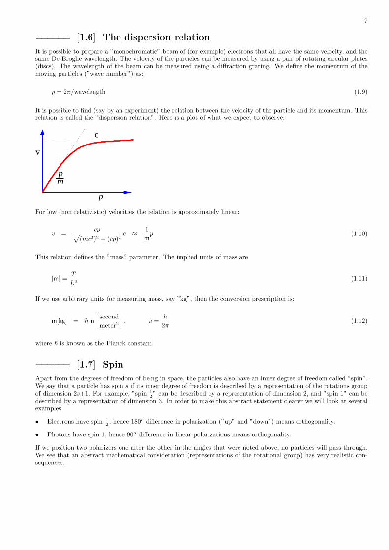
====== [1.6] The dispersion relation

It is possible to prepare a ”monochromatic” beam of (for example) electrons that all have the same velocity, and thesame De-Broglie wavelength. The velocity of the particles can be measured by using a pair of rotating circular plates(discs). The wavelength of the beam can be measured using a diffraction grating. We define the momentum of themoving particles (”wave number”) as:

p = 2π/wavelength (1.9)

It is possible to find (say by an experiment) the relation between the velocity of the particle and its momentum. Thisrelation is called the ”dispersion relation”. Here is a plot of what we expect to observe:

c

p

v

p

m

For low (non relativistic) velocities the relation is approximately linear:

v =cp√

(mc2)2 + (cp)2c ≈ 1

mp (1.10)

This relation defines the ”mass” parameter. The implied units of mass are

[m] =T

L2(1.11)

If we use arbitrary units for measuring mass, say ”kg”, then the conversion prescription is:

m[kg] = ~m[

second

meter2

], ~ =

h

2π(1.12)

where ~ is known as the Planck constant.

====== [1.7] Spin

Apart from the degrees of freedom of being in space, the particles also have an inner degree of freedom called ”spin”.We say that a particle has spin s if its inner degree of freedom is described by a representation of the rotations groupof dimension 2s+1. For example, ”spin 1

2” can be described by a representation of dimension 2, and ”spin 1” can bedescribed by a representation of dimension 3. In order to make this abstract statement clearer we will look at severalexamples.

• Electrons have spin 12 , hence 180o difference in polarization (”up” and ”down”) means orthogonality.

• Photons have spin 1, hence 90o difference in linear polarizations means orthogonality.

If we position two polarizers one after the other in the angles that were noted above, no particles will pass through.We see that an abstract mathematical consideration (representations of the rotational group) has very realistic con-sequences.

8

[2] Digression: The classical description of nature

====== [2.1] The electromagnetic field

The electric field E and the magnetic field B can be derived from the vector potential A and the electric potential V :

E = −∇V − 1

c

∂ ~A

∂t(2.1)

B = ∇× ~A

The electric potential and the vector potential are not uniquely determined, since the electric and the magnetic fieldsare not affected by the following changes:

V 7→ V = V − 1

c

∂Λ

∂t(2.2)

A 7→ A = A+∇Λ

where Λ(x, t) is an arbitrary scalar function. Such a transformation of the potentials is called ”gauge”. A special caseof ”gauge” is changing the potential V by an addition of a constant.

Gauge transformations do not affect the classical motion of the particle since the equations of motion contain onlythe derived fields E ,B.

d2x

dt2=

1

m

[eE − e

cB × x

](2.3)

This equation of motion can be derived from the Lagrangian:

L(x, x) =1

2mx2 +

e

cxA(x, t)− eV (x, t) (2.4)

Or, alternatively, from the Hamiltonian:

H(x, p) =1

2m(p− e

cA)2 + eV (2.5)

====== [2.2] The Lorentz Transformation

The Lorentz transformation takes us from one reference frame to the other. A Lorentz boost can be written in matrixform as:

S =

γ −γβ 0 0−γβ γ 0 0

0 0 1 00 0 0 1

(2.6)

where β is the velocity of our reference frame relative to the reference frame of the lab, and

γ =1√

1− β2(2.7)

9

We use units such that the speed of light is c = 1. The position of the particle in space is:

x =

txyz

(2.8)

and we write the transformations as:

x′ = Sx (2.9)

We shall see that it is convenient to write the electromagnetic field as:

F =

0 E1 E2 E3E1 0 B3 −B2

E2 −B3 0 B1

E3 B2 −B1 0

(2.10)

We shall argue that this transforms as:

F ′ = SFS−1 (2.11)

or in terms of components:

E ′1 = E1 B′1 = B1

E ′2 = γ(E2 − βB3) B′2 = γ(B2 + βE3)E ′3 = γ(E3 + βB2) B′3 = γ(B3 − βE2)

====== [2.3] Momentum and energy of a particle

Let us write the displacement of the particle as:

dx =

dtdxdydz

(2.12)

We also define the proper time (as measured in the particle frame) as:

dτ2 = dt2 − dx2 − dy2 − dz2 = (1− vx2 − vy2 − vz2)dt2 (2.13)

or:

dτ =√

1− v2dt (2.14)

The relativistic velocity vector is:

u =dx

dτ, [u2

t − u2x − u2

y − u2z = 1] (2.15)

10

It is customary to define the non-canonical momentum as

p = mu =

εpxpypz

(2.16)

According to the above equations we have:

ε2 − p2x − p2

y − p2z = m2 (2.17)

and write the dispersion relation:

ε =√

m2 + p2 (2.18)

v =p√

m2 + p2

We note that for non-relativistic velocities pi ≈ mvi for i = 1, 2, 3 while:

ε = mdt

dτ=

m√1− v2

≈ m +1

2mv2 + . . . (2.19)

====== [2.4] Equations of motion for a particle

The non-relativistic equations of motion for a particle in an electromagnetic field are:

md~v

dt= eE − eB × ~v (2.20)

The right hand side is the so-called Lorentz force ~f . It gives the rate of change of the non-canonical momentum. Therate of change of the associated non-canonical energy E is

dε

dt= ~f · ~v = eE · ~v (2.21)

The electromagnetic field has equations of motion of its own: the Maxwell equations. We shall see shortly thatMaxwell equations are Lorentz invariant. But what Newton’s second law as written above is not Lorentz invariant.In order for the Newtonian equations of motion to be Lorentz invariant we have to adjust them. It is not difficult tosee that the obvious required revision is:

mdu

dτ= eFu (2.22)

To prove the invariance under the Lorentz transformation we write:

du′

dτ=

d

dτ(Su) = S

d

dτu = S

e

mFu =

e

mSFS−1(Su) =

e

mF ′u′ (2.23)

Hence we have deduced the transformation F ′ = SFS−1 of the electromagnetic field.

11

====== [2.5] Equations of motion of the field

Back to the Maxwell equations. A simple way of writing them is

∂†F = 4πJ† (2.24)

where the derivative operator ∂, and the four-current J , are defined as:

∂ =

∂∂t

− ∂∂x

− ∂∂y

− ∂∂z

∂† =

(∂

∂t,∂

∂x,∂

∂y,∂

∂z

)(2.25)

and:

J =

ρJxJyJz

J† = (ρ,−Jx,−Jy,−Jz) (2.26)

The Maxwell equations are invariant because J and ∂ transform as vectors. For more details see Jackson. Animportant note about notations: in this section we have used what is called a ”contravariant” representation for thecolumn vectors. For example u = column(ut, ux, uy, uz). For the ”adjoint” we use the ”covariant” representationu = row(ut,−ux,−uy,−uz). Note that u†u = (ut)

2 − (ux)2 − (uy)2 − (uz)2 is a Lorentz scalar.

====== [2.6] The full Hamiltonian

The Hamiltonian that describes a system of charged particles including the electromagnetic field will be discussed ina dedicated lecture (see “special topics”). Here we just cite the bottom line expression:

H(r,p, A, E) =∑i

1

2mi(pi − eiA(ri))

2 +1

8π

∫(E2 + c2(∇×A)2)d3x (2.27)

The canonical coordinates of the particles are (r,p), and the canonical coordinates of the field are (A, E⊥). Note that

the radiation field satisfies E⊥ = −A, which is conjugate to the magnetic field B = ∇×A. The units of E as well asthe prefactor 1/(8π) are determined via Coulomb law as in the Gaussian convention. The units of B are determinedvia the Lorentz force formula as in the SI convention. Note that for the purpose if conceptual clarity we do not makethe replacement A 7→ (1/c)A, hence B and E do not have the same units.

In the absence of particles the second term of the Hamiltonian describes waves that have a dispersion relationω = c|k|. The strength of the interaction is determined by the coupling constants ei. Assuming that all the particleshave elementary charge ei = ±e, it follows that in the quantum treatment the above Hamiltonian is characterized bya single dimensionless coupling constant e2/c, which is knows as the “fine-structure constant”.

12

[3] Hilbert space

====== [3.1] Linear algebra

In Euclidean geometry, three dimensional vectors can be written as:

~u = u1~e1 + u2~e2 + u3~e3 (3.1)

Using Dirac notation we can write the same as:

|u〉 = u1|e1〉+ u2|e2〉+ u3|e3〉 (3.2)

We say that the vector has the representation:

|u〉 7→ ui =

u1

u2

u3

(3.3)

The operation of a linear operator A is written as |v〉 = A|u〉 which is represented by:

v1

v2

v3

=

A11 A12 A13

A21 A22 A23

A31 A32 A33

u1

u2

u3

(3.4)

or shortly as vi = Aijuj . Thus a linear operator is represented by a matrix:

A 7→ Aij =

A11 A12 A13

A21 A22 A23

A31 A32 A33

(3.5)

====== [3.2] Orthonormal basis

We assume that an inner product 〈u|v〉 has been defined. From now on we assume that the basis has been chosen tobe orthonormal:

〈ei|ej〉 = δij (3.6)

In such a basis the inner product (by linearity) can be calculated as follows:

〈u|v〉 = u∗1v1 + u∗2v2 + u∗3v3 (3.7)

It can also be easily proved that the elements of the representation vector can be calculated as follows:

uj = 〈ej |u〉 (3.8)

And for the matrix elements we can prove:

Aij = 〈ei|A|ej〉 (3.9)

13

====== [3.3] Completeness of the basis

In Dirac notation the expansion of a vector is written as:

|u〉 = |e1〉〈e1|u〉+ |e2〉〈e2|u〉+ |e3〉〈e3|u〉 (3.10)

which implies

1 = |e1〉〈e1|+ |e2〉〈e2|+ |e3〉〈e3| (3.11)

Above 1 7→ δij stands for the identity operator, and P j = |ej〉〈ej | are called ”projector operators”,

1 7→

1 0 00 1 00 0 1

, P 1 7→

1 0 00 0 00 0 0

, P 2 7→

0 0 00 1 00 0 0

, P 3 7→

0 0 00 0 00 0 1

, (3.12)

Now we can define the ”completeness of the basis” as the requirement

∑j

P j =∑j

|ej〉〈ej | = 1 (3.13)

From the completeness of the basis it follows e.g. that for any operator

A =

[∑i

P i

]A

∑j

P j

=∑i,j

|ei〉〈ei|A|ej〉〈ej | =∑i,j

|ei〉Aij〈ej | (3.14)

====== [3.4] Operators

In what follows we are interested in ”normal” operators that are diagonal in some orthonormal basis. Say that wehave an operator A. By definition, if it is normal, there exists an orthonormal basis |a〉 such that A is diagonal.Hence we write

A =∑a

|a〉a〈a| =∑a

aP a (3.15)

In matrix representation it means:

a1 0 00 a2 00 0 a3

= a1

1 0 00 0 00 0 0

+ a2

0 0 00 1 00 0 0

+ a3

0 0 00 0 00 0 1

(3.16)

It is useful to define what is meant by B = f(A) where f() is an arbitrary function. Assuming that A =∑|a〉a〈a|, it

follows by definition that B =∑|a〉f(a)〈a|. Another useful rule to remember is that if A|k〉 = B|k〉 for some complete

basis k, then it follows by linearity that A|ψ〉 = B|ψ〉 for any vector, and therefore A = B.

With any operator A, we can associate an “adjoint operator” A†. By definition it is an operator that satisfies thefollowing relation:

〈u|Av〉 = 〈A†u|v〉 (3.17)

14

If we substitute the basis vectors in the above relation we get the equivalent matrix-style definition

(A†)ij = A∗ji (3.18)

If A is normal then it is diagonal in some orthonormal basis, and then also A† is diagonal in the same basis. It followsthat a normal operator has to satisfy the necessary condition A†A = AA†. As we show below this is also a sufficientcondition for ”normality”.

We first consider Hermitian operators, and show that they are ”normal”. By definition they satisfy A† = A. If wewrite this relation in the eigenstate basis we deduce after one line of algebra that (a∗ − b)〈a|b〉 = 0, where a and b areany two eigenvalues. If follows (considering a = b) that the eigenvalues are real, and furthermore (considering a 6= b)that eigenvectors that are associate with different eigenvalues are orthogonal. This is called the spectral theorem: onecan find an orthonormal basis in which A is diagonal.

We now consider a general operator Q. Always we can write it as

Q = A+ iB, with A =1

2(Q+Q†), and B =

1

2i(Q−Q†) (3.19)

One observes that A and B are Hermitian operators. It is easily verified that Q†Q = QQ† iff AB = BA. It followsthat there is an orthonormal basis in which both A and B are diagonal, and therefore Q is a normal operator.

We see that an operator is normal iff it satisfies the commutation Q†Q = QQ† and iff it can be written as a functionf(H) of an Hermitian operator H. We can regard any H with non-degenerate spectrum as providing a specificationof a basis, and hence any other operator that is diagonal in that basis can be expressed as a function of this H.

Of particular interest are unitary operators. By definition they satisfy U†U = 1, and hence they are ”normal” andcan be diagonalized in an orthonormal basis. Hence their eigenvalues satisfy λ∗rλr = 1, which means that they can bewritten as:

U =∑r

|r〉eiϕr 〈r| = eiH (3.20)

where H is Hermitian. This is an example for the general statement that any normal operator can be written as afunction of some Hermitian operator H.

====== [3.5] Conventions regarding notations

In Mathematica there is a clear distinction between dummy indexes and fixed values. For example f(x ) = 8 meansthat f(x) = 8 for any x, hence x is a dummy index. But if x = 4 then f(x) = 8 means that only one element of thevector f(x) is specified. Unfortunately in the printed mathematical literature there are no clear conventions. Howeverthe tradition is to use notations such as f(x) and f(x′) where x and x′ are dummy indexes, while f(x0) and f(x1)where x0 and x1 are fixed values. Thus

Aij =

(2 35 7

)(3.21)

Ai0j0 = 5 for i0 = 2 and j0 = 1

Another typical example is

Tx,k = 〈x|k〉 = matrix (3.22)

Ψ(x) = 〈x|k0〉 = column (3.23)

In the first equality we regard 〈x|k〉 as a matrix: it is the transformation matrix form the position to the momentumbasis. In the second equality we regard the same object (with fixed k0) as a column, or as a ”wave-function”.

15

We shall keep the following extra convention: The ”bra” indexes would appear as subscripts (used for representation),while the ”ket” indexes would appear as superscripts (reserved for the specification of the state). For example:

Y `m(θ, ϕ) = 〈θ, ϕ|`m〉 = spherical harmonics (3.24)

ϕn(x) = 〈x|n〉 = harmonic oscillator eigenfunctions (3.25)

ψn = 〈n|ψ〉 = representation of wavefunction in the n basis (3.26)

Sometime it is convenient to use the Einstein summation convention, where summation over repeated dummy indexesis implicit. For example:

f(θ, ϕ) =∑`m

〈θ, ϕ|`m〉〈`m|f〉 = f`mY`m(θ, ϕ) (3.27)

In any case of ambiguity it is best to translate everything into Dirac notations.

====== [3.6] Change of basis

Definition of T :

Assume we have an ”old” basis and a ”new” basis for a given vector space. In Dirac notation:

old basis = |a = 1〉, |a = 2〉, |a = 3〉, . . . (3.28)

new basis = |α = 1〉, |α = 2〉, |α = 3〉, . . .

The matrix Ta,α whose columns represent the vectors of the new basis in the old basis is called the ”transformationmatrix from the old basis to the new basis”. In Dirac notation this may be written as:

|α〉 =∑a

Ta,α |a〉 (3.29)

In general, the bases do not have to be orthonormal. However, if they are orthonormal then T must be unitary andwe have

Ta,α = 〈a|α〉 (3.30)

In this section we will discuss the general case, not assuming orthonormal basis, but in the future we will always workwith orthonormal bases.

Definition of S:

If we have a vector-state then we can represent it in the old basis or in the new basis:

|ψ〉 =∑a

ψa |a〉 (3.31)

|ψ〉 =∑α

ψα |α〉

So, the change of representation can be written as:

ψα =∑a

Sα,aψa (3.32)

16

Or, written abstractly:

ψ = Sψ (3.33)

The transformation matrix from the old representation to the new representation is: S = T−1.

Similarity Transformation:

A unitary operation can be represented in either the new basis or the old basis:

ϕa =∑a

Aa,bψb (3.34)

ϕα =∑α

Aα,βψβ

The implied transformation between the representations is:

A = SAS−1 = T−1AT (3.35)

This is called a similarity transformation.

====== [3.7] Generalized spectral decompositions

Not any operator is normal: that means that not any matrix can be diagonalized by a unitary transformation. Inparticular we have sometime to deal with non-Hermitian Hamiltonian that appear in the reduced description of opensystems. For this reason and others it is important to know how the spectral decomposition can be generalized. Thegeneralization has a price: either we have to work with non-orthonormal basis or else we have to work with twounrelated orthonormal sets. The latter procedure is known as singular value decomposition (SVD).

Given a matrix A we can find its eigenvalues λr, which we assume below to be non degenerate. without making anyother assumption we can always define a set |r〉 of right eigenstates that satisfy A|r〉 = λr|r〉. We can also define aset |r〉 of left eigenstates that satisfy A†|r〉 = λ∗r |r〉. Unless A is normal, the r basis is not orthogonal, and therefore〈r|A|s〉 is not diagonal. But by considering 〈r|A|s〉 we can prove that 〈r|s〉 = 0 if r 6= s. Hence we have dual basissets, and without loss of generality we adopt a normalization convention such that

〈r|s〉 = δr,s (3.36)

so as to have the generalized spectral decomposition:

A =∑r

|r〉λr〈r| = T [diagλr] T−1 (3.37)

where T is the transformation matrix whose columns are the right eigenvectors, while the rows of T−1 are theleft eigenvectors. In the standard decomposition method A is regarded as describing stretching/squeezing in someprincipal directions, where T is the transformation matrix. The SVD procedure provides a different type of decom-positions. Within the SVD framework A is regarded as a sequence of 3 operations: a generalized ”rotation” followedby stretching/squeezing, and another generalized ”rotation”. Namely:

A =∑r

|Ur〉√pr〈Vr| = U

√diagprV † (3.38)

Here the positive numbers pr are called singular values, and Ur and Vr are not dual bases but unrelated orthonormalsets. The corresponding unitary transformation matrices are U and V .

17

====== [3.8] The separation of variables theorem

Assume that the operator H commutes with an Hermitian operator A. It follows that if |a, ν〉 is a basis in which Ais diagonalized, then the operator H is block diagonal in that basis:

〈a, ν|A|a′, ν′〉 = aδaa′δνν′ (3.39)

〈a, ν|H|a′, ν′〉 = δaa′H(a)νν′ (3.40)

where the top index indicates which is the block that belongs to the eigenvalue a.To make the notations clear consider the following example:

A =

2 0 0 0 00 2 0 0 00 0 9 0 00 0 0 9 00 0 0 0 9

H =

5 3 0 0 03 6 0 0 00 0 4 2 80 0 2 5 90 0 8 9 7

H(2) =

(5 33 6

)H(9) =

4 2 82 5 98 9 7

(3.41)

Proof: [H, A] = 0 (3.42)

〈a, ν|HA−AH|a′, ν′〉 = 0

a′〈a, ν|H|a′, ν′〉 − a〈a, ν|H|a′, ν′〉 = 0

(a− a′)Haν,a′ν′ = 0

a 6= a′ ⇒ Haν,a′ν′ = 0

〈a, ν|H|a′, ν′〉 = δaa′ H(a)νν′

It follows that there is a basis in which both A and H are diagonalized. This is because we can diagonalize thematrix H block by block (the diagonalizing of a specific block does not affect the rest of the matrix).

====== [3.9] Separation of variables - examples

The best know examples for “separation of variables” are for the Hamiltonian of a particle in a centrally symmetricfield in 2D and in 3D. In the first case Lz is constant of motion while in the second case both L2 and Lz are constantsof motion. The separation of the Hamiltonian into blocks is as follows:

Central symmetry in 2D:

standard basis = |x, y〉 = |r, ϕ〉 (3.43)

constant of motion = Lz (3.44)

basis for separation = |m, r〉 (3.45)

〈m, r|H|m′, r′〉 = δm,m′ H(m)r,r′ (3.46)

The original Hamiltonian and its blocks:

H =1

2p2 + V (r) =

1

2

(p2r +

1

r2L2z

)+ V (r) (3.47)

H(m) =1

2p2r +

m2

2r2+ V (r) where p2

r 7→ −1

r

∂

∂r

(r∂

∂r

)(3.48)

18

Central symmetry in 3D:

standard basis = |x, y, z〉 = |r, θ, ϕ〉 (3.49)

constants of motion = L2, Lz (3.50)

basis for separation = |`m, r〉 (3.51)

〈`m, r|H|`′m′, r′〉 = δ`,`′ δm,m′ H(`m)r,r′ (3.52)

The original Hamiltonian and its blocks:

H =1

2p2 + V (r) =

1

2

(p2r +

1

r2L2

)+ V (r) (3.53)

H(`m) =1

2p2r +

`(`+ 1)

2r2+ V (r) where p2

r 7→ −1

r

∂2

∂r2r (3.54)

19

[4] A particle in an N site system

====== [4.1] N site system

A site is a location where a particle can be positioned. If we have N = 5 sites it means that we have a 5-dimensionalHilbert space of quantum states. Later we shall assume that the particle can ”jump” between sites. For mathematicalreasons it is conveneint to assume torus topology. This means that the next site after x = 5 is x = 1. This is alsocalled periodic boundary conditions.

The standard basis is the position basis. For example: |x〉 with x = 1, 2, 3, 4, 5. So we can define the position operatoras follows:

x|x〉 = x|x〉 (4.1)

In this example we get:

x 7→

1 0 0 0 00 2 0 0 00 0 3 0 00 0 0 4 00 0 0 0 5

(4.2)

The operation of this operator on a state vector is for example:

|ψ〉 = 7|3〉+ 5|2〉 (4.3)

x|ψ〉 = 21|3〉+ 10|2〉

====== [4.2] Translation operators

The one-step translation operator is defined as follows:

D|x〉 = |x+ 1〉 (4.4)

For example:

D 7→

0 0 0 0 11 0 0 0 00 1 0 0 00 0 1 0 00 0 0 1 0

(4.5)

and hence D|1〉 = |2〉 and D|2〉 = |3〉 and D|5〉 = |1〉. Let us consider the superposition:

|ψ〉 =1√5

[|1〉+ |2〉+ |3〉+ |4〉+ |5〉] (4.6)

It is clear that D|ψ〉 = |ψ〉. This means that ψ is an eigenstate of the translation operator (with eigenvalue ei0). Thetranslation operator has other eigenstates that we will discuss in the next section.

20

====== [4.3] Momentum states

The momentum states are defined as follows:

|k〉 → 1√N

eikx (4.7)

k =2π

Nn, n = integer mod (N)

In the previous section we have encountered the k = 0 momentum state. In Dirac notation this is written as:

|k〉 =∑x

1√N

eikx|x〉 (4.8)

or equivalently as:

〈x|k〉 =1√N

eikx (4.9)

while in old fashioned notation it is written as:

ψkx = 〈x|k〉 (4.10)

where the upper index k identifies the state, and the lower index x is the representation index. Note that if x werecontinuous then it would be written as ψk(x).

The k states are eigenstates of the translation operator. This can be proved as follows:

D|k〉 =∑x

D|x〉〈x|k〉 =∑x

|x+ 1〉 1√N

eikx =∑x′

|x′〉 1√N

eik(x′−1) = e−ik∑x′

|x′〉 1√N

eikx′

= e−ik|k〉 (4.11)

Hence we get the result:

D|k〉 = e−ik|k〉 (4.12)

and conclude that |k〉 is an eigenstate of D with an eigenvalue e−ik. Note that the number of independent eigenstatesis N . For exmaple for a 5-site system we have eik6 = eik1 .

====== [4.4] Momentum operator

The momentum operator is defined as follows:

p|k〉 ≡ k|k〉 (4.13)

From the relation D|k〉 = e−ik|k〉 it follows that D|k〉 = e−ip|k〉. Therefore we deduce the operator identity:

D = e−ip (4.14)

We can also define 2-step, 3-step, and a-step translation operators as follows:

D(2) = (D)2 = e−i2p (4.15)

D(3) = (D)3 = e−i3p

D(a) = (D)a = e−iap

21

[5] The continuum limit

====== [5.1] Definition of the Wave Function

Below we will consider a site system in the continuum limit. ε→ 0 is the distance between the sites, and L is the lengthof the system. So, the number of sites is N = L/ε→∞. The eigenvalues of the position operator are xi = ε× integer.We use the following recipe for changing a sum into an integral:

∑i

7→∫dx

ε(5.1)

|2>|1>

The definition of the position operator is:

x|xi〉 = xi|xi〉 (5.2)

The completeness of the basis can be written as follows

1 =∑|xi〉〈xi| =

∫|x〉dx〈x| (5.3)

In order to get rid of the ε in the integration measure we have re-defined the normalization of the basis states asfollows:

|x〉 =1√ε|xi〉 [infinite norm!] (5.4)

Accordingly the orthonormality relation takes the following form,

〈x|x′〉 = δ(x− x′) (5.5)

where the Dirac delta function is defined as δ(0) = 1/ε and zero otherwise. Consequently the representation of aquantum state is:

|ψ〉 =∑i

ψi|xi〉 =

∫dxψ(x)|x〉 (5.6)

where

ψ(x) ≡ 〈x|ψ〉 =1√εψx (5.7)

Note the normalization of the ”wave function” is:

〈ψ|ψ〉 =∑x

|ψx|2 =

∫dx

ε|ψx|2 =

∫dx|ψ(x)|2 = 1 (5.8)

22

====== [5.2] Momentum States

The definition of the momentum states using this normalization convention is:

ψk(x) =1√L

eikx (5.9)

where the eigenvalues are:

k =2π

L× integer (5.10)

We use the following recipe for changing a sum into an integral:

∑k

7→∫

dk

2π/L(5.11)

We can verify the orthogonality of the momentum states:

〈k2|k1〉 =∑x

〈k2|x〉〈x|k1〉 =∑x

ψk2x

∗ψk1x =

∫dxψk2(x)

∗ψk1(x) =

1

L

∫dxei(k1−k2)x = δk2,k1

(5.12)

The transformation from the position basis to the momentum basis is:

Ψk = 〈k|ψ〉 =∑x

〈k|x〉〈x|ψ〉 =

∫ψk(x)

∗ψ(x)dx =

1√L

∫ψ(x)e−ikxdx (5.13)

For convenience we will define:

Ψ(k) =√LΨk (5.14)

Now we can write the above relation as a Fourier transform:

Ψ(k) =

∫ψ(x)e−ikxdx (5.15)

Or, in the reverse direction:

ψ(x) =

∫dk

2πΨ(k)eikx (5.16)

====== [5.3] Translations

We define the translation operator:

D(a)|x〉 = |x+ a〉 (5.17)

We now proof the following:

Given that: |ψ〉 7→ ψ(x) (5.18)

It follows that: D(a)|ψ〉 7→ ψ(x− a) (5.19)

23

In Dirac notation we may write:

〈x|D(a)|ψ〉 = 〈x− a|ψ〉 (5.20)

This can obviously be proved easily by operating D† on the ”bra”. However, for pedagogical reasons we will alsopresent a longer proof: Given

|ψ〉 =∑x

ψ(x)|x〉 (5.21)

Then

D(a)|ψ〉 =∑x

ψ(x)|x+ a〉 =∑x′

ψ(x′ − a)|x′〉 =∑x

ψ(x− a)|x〉 (5.22)

====== [5.4] The Momentum Operator

The momentum states are eigenstates of the translation operators:

D(a)|k〉 = e−iak|k〉 (5.23)

The momentum operator is defined the same as in the discrete case:

p|k〉 = k|k〉 (5.24)

Therefore the following operator identity emerges:

D(a) = e−iap (5.25)

For an infinitesimal translation:

D(δa) = 1− iδap (5.26)

We see that the momentum operator is the generator of the translations.

====== [5.5] The differential representation

The matrix elements of the translation operator are:

〈x|D(a)|x′〉 = δ((x− x′)− a) (5.27)

For an infinitesimal translation we write:

〈x|(1− iδap)|x′〉 = δ(x− x′)− δaδ′(x− x′) (5.28)

Hence we deduce:

〈x|p|x′〉 = −iδ′(x− x′) (5.29)

24

We notice that the delta function is symmetric, so its derivative is anti-symmetric. In analogy to multiplying amatrix with a column vector we write: A|Ψ〉 7→

∑j AijΨj . Let us examine how the momentum opertor operates on

a ”wavefunction”:

p|Ψ〉 7→∑x′

pxx′Ψx′ =

∫〈x|p|x′〉Ψ(x′)dx′ = (5.30)

= −i∫δ′(x− x′)Ψ(x′)dx′ = i

∫δ′(x′ − x)Ψ(x′)dx′

= −i∫δ(x′ − x)

∂

∂x′Ψ(x′)dx′ = −i ∂

∂xΨ(x)

Therefore:

p|Ψ〉 7→ −i ∂∂x

Ψ(x) (5.31)

We see that in the continuum limit the operation of p can be realized by a differential operator. Let us perform aconsistency check. We have already proved in a previous section that:

D(a)|ψ〉 7→ ψ(x− a) (5.32)

For an infinitesimal translation we have:

(1− iδap

)|ψ〉 7→ ψ(x)− δa d

dxψ(x) (5.33)

From here it follows that

〈x|p|ψ〉 = −i ddxψ(x) (5.34)

This means: the operation of p on a wavefunction is realized by the differential operator −i(d/dx).

====== [5.6] Algebraic characterization of translations

If |x〉 is an eigenstate of x with eigenvalue x, then D|x〉 is an eigenstate of x with eigenvalue x+ a. In Dirac notations:

x[D|x〉

]= (x+ a)

[D|x〉

]for any x (5.35)

We have (x+ a)D = D(x+ a), and x|x〉 = x|x〉. Therefore the above equality can be re-written as

xD|x〉 = D (x+ a)|x〉 for any x (5.36)

Therefore the following operator identity is implied:

x D = D (x+ a) (5.37)

Which can also be written as

[x, D] = aD (5.38)

25

The opposite is correct too: if an operator D fulfills the above relation with another operator x, then the former is atranslation operator with respect to the latter, where a is the translation distance.

The above characterization applies to any type of translation operators, include ”raising/lowering” operators whichare not necessarily unitary. A nicer variation of the algebraic relation that characterizes a translation operator isobtained if D is unitary:

D−1xD = x+ a (5.39)

If we write the infinitesimal version of this operator relation, by substituting D(δa) = 1− iδap and expanding to thefirst order, then we get the following commutation relation:

[x, p] = i (5.40)

The commutation relations allow us to understand the operation of operators without having to actually use them onwave functions.

====== [5.7] Particle in a 3D space

Up to now we have discussed the representation of a a particle which is confined to move in a one dimensionalgeometry. The generalization to a system with three geometrical dimensions is straightforward:

|x, y, z〉 = |x〉 ⊗ |y〉 ⊗ |z〉 (5.41)

x|x, y, z〉 = x|x, y, z〉y|x, y, z〉 = y|x, y, z〉z|x, y, z〉 = z|x, y, z〉

We define a ”vector operator” which is actually a ”package” of three operators:

r = (x, y, z) (5.42)

And similarly:

p = (px, py, pz) (5.43)

v = (vx, vy, vz)

A = (Ax, Ay, Az)

Sometimes an operator is defined as a function of other operators:

A = A(r) = (Ax(x, y, z), Ay(x, y, z), Az(x, y, z)) (5.44)

For example A = r/|r|3. We also note that the following notation is commonly used:

p2 = p · p = p2x + p2

y + p2z (5.45)

====== [5.8] Translations in 3D space

The translation operator in 3-D is defined as:

D(a)|r〉 = |r + a〉 (5.46)

26

An infinitesimal translation can be written as:

D(δa) = e−iδaxpxe−iδay pye−iδaz pz (5.47)

= 1− iδaxpx − iδaypy − iδaz pz = 1− iδa · p

The matrix elements of the translation operator are:

〈r|D(a)|r′〉 = δ3(r− (r′ + a)) (5.48)

Consequently, the differential representation of the momentum operator is:

p|Ψ〉 7→(−i ∂∂x

Ψ,−i ∂∂y

Ψ,−i ∂∂z

Ψ

)(5.49)

or in simpler notation p|Ψ〉 7→ −i∇Ψ. We also notice that p2|Ψ〉 7→ −∇2Ψ.

27

[6] Rotations

====== [6.1] The Euclidean Rotation Matrix

The Euclidean Rotation Matrix RE(~Φ) is a 3× 3 matrix that rotates the vector r.

x′y′z′

=

(ROTATIONMATRIX

)xyz

(6.1)

The Euclidean matrices constitute a representation of dimension 3 of the rotation group. The parametrization of a

rotation is requires three numbers that are kept in a vector ~Φ. These are the rotation axis orientation (θ, ϕ), and therotation angle Φ. Namely,

~Φ = Φ~n = Φ(sin θ cosφ, sin θ sinφ, cos θ) (6.2)

An infinitesimal rotation δ~Φ can be written as:

REr = r + δ~Φ× r (6.3)

Recalling the definition of a cross product we write this formula using matrix notations:

∑j

REijrj =∑j

[δij +

∑k

δΦk εkji

]rj (6.4)

Hence we deduce that the matrix that represents an arbitrary infinitesimal rotations is

REij = δij +∑k

δΦk εkji (6.5)

To find the matrix representation for a finite rotation is more complicated. In the future we shall learn a simple recipehow to construct a matrix that represents an arbitrary large rotation around an arbitrary axis. For now we shall besatisfied in writing the matrix that represents an arbitrary large rotation around the Z axis:

R(Φ~ez) =

cos(Φ) − sin(Φ) 0sin(Φ) cos(Φ) 0

0 0 1

≡ Rz(Φ) (6.6)

Similar expressions hold for X axis and Y axis rotations. We note that ~Φ = Rz(ϕ)Ry(θ)~ez, hence by similaritytransformation it follows that

R(~Φ) = Rz(ϕ)Ry(θ)Rz(Φ)Ry(−θ)Rz(−ϕ) (6.7)

This shows that it is enough to know the rotations matrices around Y and Z to construct any other rotation matrix.However, this is not an efficient way to construct rotation matrices. Optionally a rotation matrice can be parameterizedby its so-called ”Euler angles”

R(~Φ) = Rz(α) Rx(β) Rz(γ) (6.8)

28

This reflects the same idea (here we use the common ZXZ convention). To find the Euler angles can be complicated,and the advantage is not clear.

====== [6.2] The Rotation Operator Over the Hilbert Space

The rotation operator over the Hilbert space is defined (in analogy to the translation operator) as:

R(~Φ)|r〉 ≡ |RE(~Φ)r〉 (6.9)

This operator operates over an infinite dimension Hilbert space (the standard basis is an infinite number of ”sites” inthe three-dimensional physical space). Therefore, it is represented by an infinite dimension matrix:

Rr′r = 〈r′|R|r〉 = 〈r′|REr〉 = δ(r′ −REr) (6.10)

That is in direct analogy to the translation operator which is represented by the matrix:

Dr′r = 〈r′|D|r〉 = 〈r′|r + a〉 = δ(r′ − (r + a)) (6.11)

Both operators R and D can be regarded as ”permutation operators”. When they act on some superposition (rep-resented by a ”wavefunction”) their effect is to shift it somewhere else. As discussed in a previous section if awavefunction ψ(r) is translated by D(a) then it becomes ψ(r− a). In complete analogy,

Given that: |ψ〉 7→ ψ(r) (6.12)

It follows that: R(Φ)|ψ〉 7→ ψ(RE(−Φ)r) (6.13)

====== [6.3] Which Operator is the Generator of Rotations?

The generator of rotations (the ”angular momentum operator”) is defined in analogy to the definition of the generatorof translations (the ”linear momentum operator”). In order to define the generator of rotations around the axis n wewill look at an infinitesimal rotation of an angle δΦ~n. An infinitesimal rotation is written as:

R(δΦ~n) = 1− iδΦLn (6.14)

Below we will prove that the generator of rotations around the axis n is:

Ln = ~n · (r× p) (6.15)

where:

r = (x, y, z) (6.16)

p = (px, py, pz)

Proof: We shall show that both sides of the equation give the same result if they operate on any basis state |r〉. Thismeans that we have an operator identity.

R(δ~Φ)|r〉 = |RE( ~δΦ)r〉 = |r + δ~Φ× r〉 = D(δ~Φ× r)|r〉 (6.17)

= [1− i(δ~Φ× r) · p]|r〉 = [1− ip · δ~Φ× r]|r〉 = [1− ip · δ~Φ× r]|r〉

29

So we get the following operator identity:

R(δ~Φ) = 1− ip · δ~Φ× r (6.18)

Which can also be written (by exploiting the cyclic property of the triple vectorial multiplication):

R(δ~Φ) = 1− iδ~Φ · (r× p) (6.19)

From here we get the desired result. Note: The more common procedure to derive this identity is based on expandingthe rotated wavefunction ψ(RE(−δΦ)r) = ψ(r − δΦ× r), and exploiting the association p 7→ −i∇.

====== [6.4] Algebraic characterization of rotations

A unitary operator D realizes a translation a in the basis which is determined by an observable x if we have theequality D−1xD = x+ a. Let us prove the analogous statement for rotations: A unitary operator R realizes rotationΦ in the basis which is determined by an observable r if we have the equality

R−1riR =∑j

REij rj (6.20)

where RE is the Euclidean rotation matrix. This relation constitutes an algebraic characterization of the rotationoperator. As a particular example we write the characterization of an operator that induce 90o rotation around theZ axis:

R−1xR = −y, R−1yR = x, R−1zR = z (6.21)

This should be contrasted, say, with the characterization of translation in the X direction:

D−1xD = x+ a, D−1yD = y, D−1zD = z (6.22)

Proof: The proof of the general statement with regard to the algebraic characterization of the rotation operator istotally analogous to that in the case of translations. We first argue that R is a rotation operator iff

R|r〉 = |REr〉 for any r (6.23)

This implies that

ri

[R|r〉

]=

∑j

REijrj

[R|r〉

]for any r (6.24)

By the same manipulation as in the case of translations we deduce that

ri R |r〉 =∑j

REij R rj |r〉 for any r (6.25)

From here, operating on both sides with R−1, we get the identity that we wanted to prove.

30

====== [6.5] The algebra of the generators of rotations

Going on in complete analogy with the case of translations we write the above algebraic characterization for aninfinitesimal rotation:

[1 + iδΦjLj ] ri [1− iδΦjLj ] = ri + εijk δΦj rk (6.26)

where we used the Einstein summation convention. We deduce that

[Lj , ri] = −i εijk rk (6.27)

Thus we deduce that in order to know if a set of operators (Jx, Jy, Jz) generate rotations of eigenstates of a 3-componentobservable A, we have to check whether the following algebraic relation is satisfied:

[Ji, Aj ] = i εijk Ak (6.28)

Note that for a stylistic convenience we have interchanged the order of the indexes. In particular we deduce that thealgebra that characterized the generators of rotations is

[Ji, Jj ] = i εijk Jk (6.29)

This is going to be the starting point for constructing other representations of the rotation group.

====== [6.6] Scalars, Vectors, and Tensor Operators

We can classify operators according to the way that they transform under rotations. The simplest possibility is ascalar operator C. It has the defining property

R−1CR = C, for any rotation (6.30)

which means that

[Ji, C] = 0 (6.31)

Similarly the defining property of a vector is

R−1AiR = REijAj for any rotation (6.32)

or equivalently

[Ji, Aj ] = iεijkAk (6.33)

The generalization of this idea leads to the notion of a tensor. A multi-component observer is a tensor of rank `, if ittransforms according to the R`ij representation of rotations. Hence a tensor of rank ` should have 2`+ 1 components.In the special case of a 3-component ”vector”, as discussed above, the transformation is done using the Euclideanmatrices REij .

It is easy to prove that if A and B are vector operators, then C = A · B is a scalar operator. We can prove it eitherdirectly, or by using the commutation relations. The generalization of this idea to tensors leads to the notion of”contraction of indices”.

31

====== [6.7] Wigner-Eckart Theorem

If we know the transformation properties of an operator, it has implications on its matrix elements. This sectionassumes that the student is already familiar with the representations of the rotation group.

Let us assume that the representation of the rotations over our Hilbert (sub)space is irreducible of dimensiondim=2j+1. The basis states are |m〉 with m = −j...+ j. Let us see what are the implications with regard toscalar and vector operators.

The representation of a scalar operator C should be trivial, i.e. proportional to the identity, i.e. a ”constant”:

Cm′m = c δm′m within a given j irreducible subspace (6.34)

else it would follow from the “separation of variables theorem” that all the generators (Ji) are block-diagonal in thesame basis. Note that within the pre-specified subspace we can write c = 〈C〉, where the expectation value can betaken with any state.

A similar theorem applies to a vector operator A. Namely,

[Ak]m′m = g × [Jk]m′m within a given j irreducible subspace (6.35)

How can we determine the coefficient g? We simply observe that from the last equation it follows that

[A · J ]m′m = g [J2]m′m = g j(j + 1) δm′m (6.36)

in agreement with what we had claimed regarding scalars in general. Therefore we get the formula

g =〈J ·A〉j(j + 1)

(6.37)

where the expectation value of the scalar can be calculated with any state.

The direct proof of the Wigner-Eckart theorem, as e.g. in Cohen-Tannoudji, is extremely lengthy. Here we propose avery short proof that can be regarded as a variation on what we call the ”separation of variable theorem”.

Proof step (1): From [Ax, Jx] = 0 we deduce that Ax is diagonal in the Jx basis, so we can write this relationas Ax = f(Jx). The rotational invariance implies that the same function f() related Ay to Jy and Az to Jz. Thisinvariance is implied by a similarity transformation and using the defining algebraic property of vector operators.

Proof step (2): Next we realize that for a vector operator [Jz, A+] = A+ where A+ = Ax + iAy. It follows that A+

is a raising operator in the Jz basis, and therefore must be expressible as A+ = g(Jz)[Jx + iJy], where g() is somefunction.

Proof step (3): It is clear that the only way to satisfy the equality f(Jx) + if(Jy) = g(Jz)[Jx + iJy], is to havef(X) = gX and g(X) = g, where g is a constant. Hence the Wigner-Eckart theorem is proved.

32

Fundamentals (part II)

[7] Quantum states / EPR / Bell / postulates

====== [7.1] The two slit experiment

If we have a beam of electrons, that have been prepared with a well defined velocity, and we direct it to a screenthrough two slits, then we get an interference pattern from which we can determine the ”de-Broglie wavelength” ofthe electrons. I will assume that the student is familiar with the discussion of this experiment from introductorycourses. The bottom line is that the individual electrons behave like wave and can be characterized by a wavefunctionψ(x). This by itself does not mean that our world in not classical. We still can speculate that ψ(x) has a classicalinterpenetration. Maybe our modeling of the system is not detailed enough. Maybe the two slits, if they are bothopen, deform the space in a special way that makes the electrons likely to move only in specific directions? Maybe,if we had better experimental control, we could predict with certainty where each electron will hit the screen.

The modern interpenetration of the two slit experiment is not classical. The so called ”quantum picture” is that theelectron can be at the same time at two different places: it goes via both slits and interferes with itself. This soundsstrange.

Whether the quantum interpenetration is correct we cannot establish: maybe in the future we will have a differenttheory. What we can establish is that a classical interpretation of reality is not possible. This statement is based ona different type of an experiment that we discuss below.

====== [7.2] Is the world classical? (EPR, Bell)

We would like to examine whether the world we live in is “classical” or not. The notion of classical world includesmainly two ingredients: (i) realism (ii) determinism. By realism we means that any quantity that can be measuredis well defined even if we do not measure it in practice. By determinism we mean that the result of a measurementis determined in a definite way by the state of the system and by the measurement setup. We shall see later thatquantum mechanics is not classical in both respects: In the case of spin 1/2 we cannot associate a definite value ofσy for a spin which has been polarized in the σx direction. Moreover, if we measure the σy of a σx polarized spin, weget with equal probability ±1 as the result.

In this section we would like to assume that our world is ”classical”. Also we would like to assume that interactionscannot travel faster than light. In some textbooks the latter is called ”locality of the interactions” or ”causality”. Ithas been found by Bell that the two assumptions lead to an inequality that can be tested experimentally. It turnsout from actual experiments that Bell’s inequality are violated. This means that our world is either non-classical orelse we have to assume that interactions can travel faster than light.

If the world is classical it follows that for any set of initial conditions a given measurement would yield a definiteresult. Whether or not we know how to predict or calculate the outcome of a possible measurement is not assumed.To be specific let us consider a particle of zero spin, which disintegrates into two particles going in opposite directions,each with spin 1/2. Let us assume that each spin is described by a set of state variables.

state of particle A = xA1 , xA2 , ... (7.1)

state of particle B = xB1 , xB2 , ...

The number of state variables might be very big, but it is assumed to be a finite set. Possibly we are not aware ornot able to measure some of these “hidden” variables.

Since we possibly do not have total control over the disintegration, the emerging state of the two particles is describedby a joint probability function ρ

(xA1 , ..., x

B1 , ...

). We assume that the particles do not affect each other after the

disintegration (“causality” assumption). We measure the spin of each of the particles using a Stern-Gerlach apparatus.The measurement can yield either 1 or −1. For the first particle the measurement outcome will be denoted as a,

33

and for the second particle it will be denoted as b. It is assumed that the outcomes a and b are determined in adeterministic fashion. Namely, given the state variables of the particle and the orientation θ of the apparatus we have

a = f(θA, xA1 , x

A2 , ...) = ±1 (7.2)

b = f(θB , xB1 , x

B2 , ...) = ±1

where the function f() is possibly very complicated. If we put the Stern-Gerlach machine in a different orientationthen we will get different results:

a′ = f(θ′A, x

A1 , x

A2 , ...

)= ±1 (7.3)

b′ = f(θ′B , x

B1 , x

B2 , ...

)= ±1

We have the following innocent identity:

ab+ ab′ + a′b− a′b′ = ±2 (7.4)

The proof is as follows: if b = b′ the sum is ±2a, while if b = −b′ the sum is ±2a′. Though this identity looks innocent,it is completely non trivial. It assumes both ”reality” and ”causality”. The realism is reflected by the assumptionthat both a and a′ have definite values, as implied by the function f(), even if we do not measure them. In theclassical context it is not an issue whether there is a practical possibility to measure both a and a′ at a single run ofthe experiment. As for the causality: it is reflected by assuming that a depends on θA but not on the distant setupparameter θB .

Let us assume that we have conducted this experiment many times. Since we have a joint probability distribution ρ,we can calculate average values, for instance:

〈ab〉 =

∫ρ(xA1 , ..., x

B1 , ...

)f(θA, x

A1 , ...

)f(θB , x

B1 , ...

)(7.5)

Thus we get that the following inequality should hold:

|〈ab〉+ 〈ab′〉+ 〈a′b〉 − 〈a′b′〉| ≤ 2 (7.6)

This is called Bell’s inequality (in fact it is a variation of the original version). Let us see whether it is consistent withquantum mechanics. We assume that all the pairs are generated in a singlet (zero angular momentum) state. It isnot difficult to calculate the expectation values. The result is

〈ab〉 = − cos(θA − θB) ≡ C(θA − θB) (7.7)

we have for example

C(0o) = −1, C(45o) = − 1√2, C(90o) = 0, C(180o) = +1. (7.8)

If the world were classical the Bell’s inequality would imply

|C(θA − θB) + C(θA − θ′B) + C(θ′A − θB)− C(θ′A − θ′B)| ≤ 2 (7.9)

Let us take θA = 0o and θB = 45o and θ′A = 90o and θ′B = −45o. Assuming that quantum mechanics holds we get

∣∣∣∣(− 1√2

)+

(− 1√

2

)+

(− 1√

2

)−(

+1√2

)∣∣∣∣ = 2√

2 > 2 (7.10)

34

It turns out, on the basis of celebrated experiments that Nature has chosen to violate Bell’s inequality. Furthermoreit seems that the results of the experiments are consistent with the predictions of quantum mechanics. Assuming thatwe do not want to admit that interactions can travel faster than light it follows that our world is not classical.

====== [7.3] Optional tests of realism

Mermin and Greenberger-Horne-Zeilinger have proposed optional tests for realism. The idea is to show that thefeasibility of preparing some quantum states cannot be explained within the framework of a classical theory. Weprovide below two simple examples. The spin 1/2 mathematics that is required to understand these examples will bediscussed in later lecture. What we need below is merely the following identities that express polarizations in the Xand Y directions as a superposition of polarizations in the Z direction:

|x〉 =1√2

(|z〉+ |z〉) (7.11)

|x〉 =1√2

(|z〉 − |z〉) (7.12)

|y〉 =1√2

(|z〉+ i|z〉) (7.13)

|y〉 =1√2

(|z〉 − i|z〉) (7.14)

We use the notations |z〉 and |z〉 for denoting ”spin up” and ”spin down” in Z polarization measurement, and similarconvection for polarization measurement in the other optional directions X and Y.

Three spin example.– Consider 3 spins that are prepared in the following superposition state:

|ψ〉 =1√2

(| ↑↑↑〉 − | ↓↓↓〉) ≡ 1√2

(|zzz〉 − |zzz〉) (7.15)

If we measure the polarization of 3 spins we get a = ±1 and b = ±1 and c = ±1, and the product would beC = abc = ±1. If the the measurement is in the ZZZ basis the result might be either CZZZ = +1 or CZZZ = −1with equal probabilities. But optionally we can perform an XXX measurement or XYY, or YXY, or YYX measure-ment. If for example we perform XYY measurement it is useful to write the state in the XYY basis:

|ψ〉 =1

2(|xyy〉+ |xyy〉+ |xyy〉+ |xyy〉) (7.16)

We see that the product of polarization is always CXY Y = +1. Similarly one can show that CY XY = +1 andCY Y X = +1. If the world were classical we could predict the result of an XXX measurement:

CXXX = axbxcx = ax bx cx a2y b

2y c

2y = CXY Y CY XY CY Y X = 1 (7.17)

But quantum theory predicts a contradicting result. To see what is the expected result we write the state in the XXXbasis:

|ψ〉 =1

2(|xxx〉+ |xxx〉+ |xxx〉+ |xxx〉) (7.18)

We see that the product of polarization is always CXXX = −1. Thus, the experimental feasibility of preparing suchquantum state contradicts classical realism.

35

Two spin example.– Consider 2 spins that are prepared in the following superposition state:

|ψ〉 =1√3

(|zz〉+ |zz〉 − |zz〉) (7.19)

=1√6

(|zx〉 − |zx〉+ 2|zx〉) (7.20)

=1√6

(|xz〉 − |xz〉+ 2|xz〉) (7.21)

=1√12

(|xx〉+ |xx〉+ |xx〉 − 3|xx〉) (7.22)

Above we wrote the state in the optional bases ZZ and ZX and XZ and XX. By inspection we see the following:(1) The ZZ measurement result |zz〉 is impossible.(2) The ZX measurement result |zx〉 is impossible.(3) The XZ measurement result |xz〉 is impossible.(4) All XX measurement results are possible with finite probability.

We now realize that in a classical reality observation (4) is in contradiction with observations (1-3). The argument isas follow: in each run of the experiment the state ~a = (ax, az) of the first particle is determined by some set of hidden

variables. The same applies with regard to the ~b = (bx, bz) of the second particle. We can define a joint probability

function f(~a,~b)

that gives the probabilities to have any of the 4 × 4 possibilities (irrespective of what we measure

in practice). It is useful to draw a 4× 4 truth table and to indicate all the possibilities that are not compatible with(1-3). Then it turns out that the remaining possibilities are all characterized by having ax = −1 or bx = −1. Thismeans that in a classical reality the probability to measure |xx〉 is zero. This contradicts the quantum prediction (4).Thus, the experimental feasibility of preparing such quantum state contradicts classical realism.

====== [7.4] The notion of quantum state

A-priory we can classify the possible ”statistical states” of a prepared system as follows:

• Classical state: any measurement gives a definite value.

• Pure state: there is a complete set of measurements that give definite value, while any other measurement givesan uncertain value.

• Mixture: it is not possible to find a complete set of measurements that give a definite value.

When we go to Nature we find that classical states do not exist. The best we can get are ”pure states”. For example:

(1) The best we can have with the spin of an electron is 100% polarization (say) in the X direction, but thenany measurement in any different direction gives an uncertain result, except the −X direction which we call the”orthogonal” direction. Consequently we are inclined to postulate that polarization (say) in the non-orthogonal Zdirection is a superposition of the orthogonal X and −X states.

(2) With photons we are inclined to postulate that linear polarization in the 45o direction is a superposition of theorthogonal X polarization and Y polarization states. Note however that contrary to the electronic spin, here thesuperposition of linear polarized states can optionally give different type of polarization (circular / elliptic).

(3) With the same reasoning, and on the basis of the “two slit experiment” phenomenology, we postulate that aparticle can be in a superposition state of two different locations. The subtlety here is that superposition of differentlocations is not another location but rather (say) a momentum state, while superposition of different polarizationsstates is still another polarization state.

Having postulated that all possible pure states can be regarded as forming an Hilbert space, it still does not helpus to define the notion of quantum state in the statistical sense. We need a second postulate that would imply thefollowing: If a full set of measurements is performed (in the statistical sense), then one should be able to predict (inthe statistical sense) the result of any other measurement.

36

Example: In the case of spins 1/2, say that one measures the average polarization Mi in the i = X,Y, Z directions.Can one predict the result for Mn, where n is a unit vector pointing in an arbitrary direction? According to the secondpostulate of quantum mechanics (see next section) the answer is positive. Indeed experiments reveal that Mn = n ·M .Taking together the above two postulates, our objective would be to derive and predict such linear relations from ourconception of Hilbert space. In the spin 1/2 example we would like to view Mn = n ·M as arising from the dim=2representation of the rotation group. Furthermore, we would like to derive more complicated relations that wouldapply to other representations (higher spins).

====== [7.5] The four Postulates of Quantum Mechanics

The 18th century version of classical mechanics can be derived from three postulates: The three laws of Newton. Thebetter formulated 19th century version of classical mechanics can be derived from three postulates: (1) The stateof classical particles is determined by the specification of their positions and its velocities; (2) The trajectories aredetermined by an “action principle”, hence derived from a Lagrangian. (3) The form of the Lagrangian of the theoryis determined by symmetry considerations, namely Galilei invariance in the non-relativistic case. See the Mechanicsbook of Landau and Lifshitz for details.

Quantum mechanics requires four postulates: two postulates define the notion of quantum state, while the other twopostulates, in analogy with classical mechanics, are about the laws that govern the evolution of quantum mechanicalsystems. The four postulates are:

(1) The collection of ”pure” states is a linear space (Hilbert).

(2) The expectation values of observables obey linearity: 〈αX + βY 〉 = α〈X〉+ β〈Y 〉

(3) The evolution in time obey the superposition principle: α|Ψ0〉+ β|Φ0〉 → α|Ψt〉+ β|Φt〉

(4) The dynamics of a system is invariant under specific transformations (”gauge”, ”Galilei”).

The first postulate refers to ”pure states”. These are states that have been filtered. The filtering is called ”prepara-tion”. For example: we take a beam of electrons. Without ”filtering” the beam is not polarized. If we measure thespin we will find (in any orientation of the measurement apparatus) that the polarization is zero. On the other hand,if we ”filter” the beam (e.g. in the left direction) then there is a direction for which we will get a definite result (inthe above example, in the right/left direction). In that case we say that there is full polarization - a pure state. The”uncertainty principle” tells us that if in a specific measurement we get a definite result (in the above example, inthe right/left direction), then there are different measurements (in the above example, in the up/down direction) forwhich the result is uncertain. The uncertainty principle is implied by the first postulate.

The second postulate use the notion of ”expectation value” that refers to ”quantum measurement”. In contrast withclassical mechanics, the measurement has meaning only in a statistical sense. We measure ”states” in the followingway: we prepare a collection of systems that were all prepared in the same way. We make the measurement on all the”copies”. The outcome of the measurement is an event x = x that can be characterized by a distribution function.The single event can show that a particular outcome has a non-zero probability, but cannot provide full informationon the state of the system. For example, if we measured the spin of a single electron and get σz = 1, it does not meanthat the state is polarized ”up”. In order to know if the electron is polarized we must measure a large number ofelectrons that were prepared in an identical way. If only 50% of the events give σz = 1 we should conclude that thereis no definite polarization in the direction we measured!

====== [7.6] Observables as random variables

Observable is a random variable that can have upon measurement a real numerical value. In other words x = xis an event. Let us assume, for example, that we have a particle that can be in one of five sites: x = 1, 2, 3, 4, 5.An experimentalist could measure Prob(x = 3) or Prob(p = 3(2π/5)). Another example is a measurement of theprobability Prob(σz = 1) that the particle will have spin up.

The collection of values of x is called the spectrum of values of the observable. We make the distinction betweenrandom variables with a discrete spectrum, and random variables with a continuous spectrum. The probability

37

function for a random variable with a discrete spectrum is defined as:

f(x) = Prob(x = x) (7.23)

The probability density function for a random variable with a continuous spectrum is defined as:

f(x)dx = Prob(x < x < x+ dx) (7.24)

The expectation value of a variable is defined as:

〈x〉 =∑x

f(x)x (7.25)

where the sum should be understood as an integral∫dx in the case the x has a continuous spectrum. Of particular

importance is the random variable

P x = δx,x (7.26)

This random variable equals 1 if x = x and zero otherwise. Its expectation value is the probability to get 1, namely

f(x) = 〈P x〉 (7.27)

Note that x can be expressed as the linear combination∑x xP

x.

====== [7.7] Quantum Versus Statistical Mechanics

Quantum mechanics stands opposite classical statistical mechanics. A particle is described in classical statisticalmechanics by a probability function:

ρ(x, p)dxdp = Prob(x < x < x+ dx, p < p < p+ dp) (7.28)

Optionally this definition can be expressed as the expectation value of a phase space projector

ρ(x, p) = 〈 δ(x− x) δ(p− p) 〉 (7.29)

The expectation value of a random variable A = A(x, p) is implied:

〈A〉 =

∫A(x, p)ρ(x, p)dxdp (7.30)

From this follows the linear relation:

〈αA+ βB〉 = α〈A〉+ β〈B〉 (7.31)

We see that the linear relation of the expectation values is a trivial result of classical probability theory. It assumesthat a joint probability function can be defined. But in quantum mechanics we cannot define a ”quantum state” usinga joint probability function, as implied by the observation that our world is not “classical”. For example we cannothave both the location and the momentum well defined simultaneously: a momentum state, by definition, is spreadall over space. For this reason, we have to use a more sophisticated definition of ρ. The more sophisticated definition

38

regards ρ as set of expectation values, from which all other expectation values can be deduced, taking the linearity ofthe expectation value as a postulate.

====== [7.8] Observables as operators

In the quantum mechanical treatment we regard an observable x as an operator. Namely we define its operation onthe basis states as x|x〉 = x|x〉, and by linearity its operation is defined on any other state. We can associate with the

basis states projectors P x. For example

x 7→

1 0 00 2 00 0 3

; P 1 7→

1 0 00 0 00 0 0

; P 2 7→

0 0 00 1 00 0 0

; P 3 7→

0 0 00 0 00 0 1

; (7.32)

In order to further discuss the implications of the first two postulates of quantum mechanics it is useful to considerthe simplest example, which is spin 1/2. Motivated by the experimental context, we make the following associationsbetween random variables and operators:

σn 7→(

1 00 −1

)in the n basis

n = x, y, z or any other direction (7.33)

Optionally we can define the projectors

Pn 7→(

1 00 0

)in the n basis

n = x, y, z or any other direction (7.34)

Note that

σn = 2Pn − 1 (7.35)

It follows from the first postulate that the polarization state |n〉 can be expressed as a linear combination of, say, ”up”and ”down” polarizations. We shall see that the mathematical theory of the rotation group representation, impliesthat in the standard (up/down) basis the operators σx, σy, and σz are represented by the Pauli matrices σx, σy, andσz. We use the notations:

σx =

(0 11 0

), σy =

(0 −ii 0

), σz =

(1 00 −1

)(7.36)

Furthermore, the mathematical theory of the rotation group representation, allows us to write any σn as a linearcombination of (σx, σy, σz).

Taking a more abstract viewpoint we point out that any spin operator is represented by a 2× 2 matrix, that can bewritten as a linear combination of standard basis matrices as follows:(

a bc d

)= a

(1 00 0

)+ b

(0 10 0

)+ c

(0 01 0

)+ d

(0 00 1

)=

∑nm

AnmPmn (7.37)

In the example above we denote the basis matrices as P z, S+, S−, P−z. In general we use the notation Pmn = |n〉〈m|.Note that Pn = Pnn are projectors, while the n 6= m operators are not even hermitian, and therefore cannot beinterpreted as representing observables.

Instead of using the standard basis P z, S+, S−, P−z it is possibly more physically illuminating to take 1, σx, σy, σzas the basis set. Optionally one can take 1, P x, P y, P z or P z, P−z, P x, P y as the basis set.

39

The bottom line is that the operators that act on an N dimensional Hilbert space form an N2 dimensional space. Wecan span this space in the standard basis, but physically it is more illuminating, and always possible, to pick a basisset of N2 hermitian operators. Optionally we can pick a complete set of N2 linearly independent projectors. Thelinear relations between sets of states (as implied by the first postulate of quantum mechanics) translate into linearrelations between sets of operators. One should be careful not to abuse the latter statement: in the above examplethe projectors P x, P y, P z are linearly independent, while the associated states |x〉, |y〉, |z〉 are not.

====== [7.9] The tomography of quantum states

The first postulate of Quantum Mechanics implies that with any observable we can associate an Hermitian operatorthat belongs to the N2-dimensional space of operators. We can span the whole space of observables by any set ofN2 independent operators P r. The standard basis is not physically illuminating, because the matrices Pmn are nothermitian, and therefore cannot be associated with random variables. But without loss of generality we can alwaysassume an optional basis of hermitian matrices, possibly N2 independent projectors.

From the second postulate of Quantum mechanics it follows that if A =∑r arP

r then

〈A〉 =∑r

arρr where ρr ≡ 〈P r〉 (7.38)

The set of N2 expectation values fully characterizes the quantum state. Hence we can say the ρ represents thequantum state, in the same sense that a probability function represent a statistical state in classical mechanics. Thedetermination of the state ρ on the basis of a set of measurements is called ”quantum tomography”. It should beclear that if we know ρ we can predict the expectation value of any other measurement.

In the dim= 2 spin case any operator can be written as a linear combination of the Pauli matrices:

A = a01 + axσx + ayσy + azσz = a0 + a · σ (7.39)

It is implied by the second postulate of quantum mechanics that

〈A〉 = a0 + ax〈σx〉+ ay〈σy〉+ az〈σz〉 = a0 + a ·M (7.40)

where the polarization vector is defined as follows:

M =(〈σx〉, 〈σy〉, 〈σz〉

)(7.41)

In the general case, to be discussed below, we define a package ρ = ρr of expectation values that we call probabilitymatrix. The polarization vector M can be regarded as the simplest example for such matrix. The term “matrix” isused because in general the label r that distinguishes the N2 basis operators is composed of two indexes. We note thata measurement of a non-degenerate observable provides N−1 independent expectation values (the probabilities to getany of the possible outcomes). Accordingly quantum tomography requires the measurement of N+1 non-commutingobservables.

====== [7.10] Definition of the probability matrix

The definition of ρ in quantum mechanics is based on the trivial observation that any observable A can be written asa linear combination of N2−1 independent projectors. If we know the associated N2−1 independent probabilities, orany other set of N2−1 independent expectation values, then we can predict the result of any other measurement (inthe statistical sense). The possibility to make a prediction is based on taking the linearity of the expectation value asa postulate. The above statement is explained below, but the best is to consider the N = 2 example that comes later.

Any Hermitian operator can be written as a combination of N2 operators as follows:

A =∑n,m

|n〉〈n|A|m〉〈m| =∑n,m

Anm Pmn (7.42)

40

where Pmn = |n〉〈m|. These N2 operators are not all hermitians, and therefore, strictly speaking, they do not representa set of observables. However we can easily express them using a set of N2 hermitian observables as follows:

Pnn = Pn (7.43)

Pmn =1

2(Xr + iY r) for m>n (7.44)

Pmn =1

2(Xr − iY r) for m<n (7.45)

where r = (nm) = (mn) is a composite index that runs over the [N(N−1)/2] possible combinations of n and m. Thedefinitions of Xr and Y r are implied by the above expressions: in the dim= 2 case X and Y are called Pauli matrices,while here we shall call them generalized Pauli matrices. It is useful to notice that the generalized Pauli matrices canbe expressed as combinations of elementary Projectors. Define Qr as a projector on the state |n〉+ |m〉 and Rr as aprojector on the state |n〉+ i|m〉. Then we have:

X(nm) = 2Q(nm) − Pn − Pm (7.46)

Y (nm) = 2R(nm) − Pn − Pm (7.47)

Accordingly the set of generalized projectors Pmn, is in fact equivalent to a set of N2 proper projectors (Pn, Qr, Rr).If one can extract from measurements the associated probabilities, it becomes possible to predict the result of anyother expectation value according to the equation:

〈A〉 =∑n,m

Anm ρmn = trace(Aρ) (7.48)

where ρ is named the probability matrix. Each entry in the probability matrix is a linear combination of expectationvalues of projectors. Note that the expectation value of a projector P = |ψ〉〈ψ| is the probability to find the systemsin the state |ψ〉, while the expectation values of a generalized projector Pr is defined as (〈Xr〉 ± i〈Y r〉)/2, as impliedby the definitions above.

====== [7.11] Example: probability matrix for spin

Let us relate the two common ways in which one can specify the quantum state of a spin 1/2 entity. On possibilityis to specify the polarization vector, as discussed in previous section. The other way is to define a 2 × 2 probabilitymatrix as follows. The generalized projectors are

P↑↑ = | ↑〉〈↑ | =

(1 00 0

)=

1

2(1 + σz) = P z (7.49)

P↓↓ = | ↓〉〈↓ | =

(0 00 1

)=

1

2(1− σz) = 1− P z

P↓↑ = | ↑〉〈↓ | =

(0 10 0

)=

1

2(σx + iσy) =

1

2(2P x − 1) +

i

2(2P y − 1)

P↑↓ = | ↓〉〈↑ | =

(0 01 0

)=

1

2(σx − iσy) =

1

2(2P x − 1)− i

2(2P y − 1)

The elements of the probability matrix are the expectation values of the above generalized projectors. Consequentlywe deduce the following relation between the probability matrix and the polarization vector:

ρ = 〈P ji〉 =

(12 (1 +M3) 1

2 (M1 − iM2)12 (M1 + iM2) 1

2 (1−M3)

)=

1

2(1 + ~M · ~σ) (7.50)

41

====== [7.12] Pure states as opposed to mixed states

After diagonalization, the probability matrix can be written as:

ρ →

p1 0 0 .0 p2 0 .0 0 p3 .. . . .

..

(7.51)

The convention is to order the diagonal elements in descending order. Using the common jargon we say that the staterepresented by ρ is a mixture of |1〉, |2〉, |3〉, . . . with weights p1, p2, p3, . . .. The most well known mixed state is thecanonical state:

pr =1

Ze−βEr , β ≡ 1/T, Z ≡

∑r

e−βEr (7.52)

A ”pure state” is the special case where the probability matrix after diagonalization is of the form:

ρ →

1 0 0 .0 0 0 .0 0 0 .. . . .

..

(7.53)

This may be written in a more compact way as ρ = |1〉〈1| = |ψ〉〈ψ| = Pψ. Note that 〈Pψ〉 = 1. This means a definiteoutcome for a measurement that is aimed in checking whether the particle is in state ”1”. That is why we say thatthe state is pure.

====== [7.13] Various versions of the expectation value formula

[1] The standard version of the expectation value formula:

〈A〉 = tr(Aρ) (7.54)

[2] The ”mixture” formula:

〈A〉 =∑r

pr〈r|A|r〉 (7.55)

[3] The ”sandwich” formula:

〈A〉ψ = 〈ψ|A|ψ〉 (7.56)

[4] The ”projection” formula:

Prob(φ|ψ) = |〈φ|ψ〉|2 (7.57)

The equivalence of statements 1-4 can be proved. In particular let us see how we go from the fourth statement to thethird:

〈A〉ψ =∑a

Prob(a|ψ)a =∑a

|〈a|ψ〉|2a = 〈ψ|A|ψ〉 (7.58)

42

[8] The evolution of quantum mechanical states

====== [8.1] The Evolution Operator and the Hamiltonian

Consider a particle in an N site system. If we redefine the first basis state as |1〉 = −8|1〉 we get a non-orthonormalbasis, and therefore not convenient for practical mathematical calculations. Explanation: if we represent the state |ψ〉as a linear combination of normalized basis vectors |ψ〉 =

∑j ψj |j〉, then we can find the coefficients of the combination

by using the formula ψi = 〈i|ψ〉.

Even if we decide to work with a set of orthonormal states, still there is some freedom left which is called ”gaugefreedom” or ”phase freedom”: multiplying a state with a phase factor does not imply a different state, ρ stays thesame, and hence all physical expectation values remain the same too. Example: The spin states | ↑〉 and e

π8 i| ↑〉 are

represented by the same polarization vector, or optionally by the same ρ.

From the superposition principle, and from the above remarks regarding the normalization, it follows that the evolutionin quantum mechanics is described by a unitary operator:

|ψt=0〉 → |ψt〉 (8.1)

|ψt〉 = U |ψt=0〉

It is assumed here that the system is isolated. In order to simplify the discussion below we further assume that theexternal fields are constant in time. In such a case, the evolution operator must fulfill the following ”group property”:

U(t2 + t1) = U(t2) U(t1) (8.2)

It follows that the evolution operator can be written as

U(t) = e−itH (8.3)

where H is called the Hamiltonian or ”generator” of the evolution.

Proof: The constructive way of proving the last formula is as follows: In order to know the evolution of a systemfrom t1 to t2 we divide the time into many small intervals of equal size dt = (t2 − t1)/N . This means that:

U(t2, t1) = U(t2, t2−dt) · · · U(t1+2dt, t1 + dt) U(t1+dt, t1) (8.4)

The evolution during an infinitesimal time interval can be written as:

U(dt) ≡ 1− idtH (8.5)

where the Hamiltonian can be regarded as the ”evolution per unit of time”. Or we may say that H is the log derivativeof U with respect to time. By multiplying many infinitesimal time steps we get:

U = (1− idtH) · · · (1− idtH)(1− idtH) =

(1− i t

#stepsH)#steps

= e−itH (8.6)

where we have assumed that the Hamiltonian does not change in time, so that the multiplication of exponentscan be changed into a single exponent with a sum of powers. We have used above the definition of the expo-nential function in mathematics: exp(t) = lim(1 + t/N)N , that follows from the assumed multiplicative propertyexp(t1) exp(t2) = exp(t1 + t2).

43

====== [8.2] The Schrodinger Equation

Consider the evolution of a pure state:

ψt = Uψt=0 (8.7)

From the rerlation ψt+dt = (1− idtH)ψt it follows that

dψ

dt= −iHψ (8.8)

This is the Schrodinger equation. We have allowed ourselves above to use sloppy notations (the ”ket” has beenomitted). One should realize that the Schrodinger equation reflects the definition of the Hamiltonian as the generatorof the evolution.

We now consider the evolution of a general mixture:

ρ =∑r

|r〉pr〈r| (8.9)

we have |r〉 → U |r〉 and 〈r| → 〈r|U†, therefore the evolution of ρ in time is:

ρt = Uρt=0U† (8.10)

dρ

dt= −i[H, ρ] (8.11)

This is the Liouville von-Neumann equation. One of its advantages is that the correspondence between the formalismof statistical mechanics and quantum mechanics becomes explicit. The difference is that in quantum mechanics wedeal with a probability matrix whereas in statistical mechanics we deal with a probability function.

====== [8.3] Stationary States (the ”Energy Basis”)

We can find the eigenstates |n〉 and the eigenvalues En of a Hamiltonian, which is called diagonalization:

H|n〉 = En|n〉 (8.12)

U |n〉 = e−iEnt|n〉 (8.13)

U → δn,me−iEnt (8.14)

Using Dirac notations:

〈n|U |m〉 = δnme−iEnt (8.15)

If we prepare a superposition of basis states:

|ψt=0〉 =∑n

ψn |n〉 (8.16)

we get after time t

|ψ(t)〉 =∑n

e−iEntψn |n〉 (8.17)

44

====== [8.4] How do we construct the Hamiltonian?

We construct the Hamiltonian from ”symmetry” considerations. In the next lecture our object will be to show thatthe Hamiltonian of a non-relativistic particle is of the form:

H =1

2m(p−A(x))2 + V (x) (8.18)

In this lecture we discuss a simpler case: the Hamiltonian of a particle in a two-site system. We make the followingassumptions about the two-site dynamics:

• The system is symmetric with respect to reflection.• The particle can move from site to site.

These two assumptions determine the form of the Hamiltonian. In addition, we will see how ”gauge” considerationscan make the Hamiltonian simpler, without loss of generality.

In advance we note that because of gauge considerations, the Hamiltonian can only be determined up to a constant.

H → H+ ε01 (8.19)

Namely, if we add a constant to a Hamiltonian, then the evolution operator only changes by a global phase factor:

U(t) → e−it(H+ε01) = e−iε0t e−itH (8.20)

This global phase factor can be gauged away by means of time dependent gauge transformation. We shall discussgauge transformations in the next sections.

====== [8.5] The Hamiltonian of a two-site system

It would seem that the most general Hamiltonian for a particle in a two-site system includes 4 parameters:

H =

(ε1 ce−iφ

ceiφ ε2

)(8.21)

The first observation is that thanks to gauge freedom we can define a new basis such that φ = 0. The new basis is

|1〉 = |1〉 (8.22)

|2〉 = eiφ|2〉

and we see that:

〈2|H|1〉 = e−iφ〈2|H|1〉 = e−iφceiφ = c (8.23)

Next we can make change the Hamiltonian by a constant ε1. This can be regarded as gauge transformation in time.This means that the basis in time t is identified as |1〉 = exp(−iε1t)|1〉 and |2〉 = exp(−iε1t)|2〉. In this time dependentbasis the diagonal matrix elements of the Hamiltonian becomes 0 instead of ε1, and ε = ε2 − ε1 instead of ε2. It should

45

be emphasized that on physical grounds one cannot say whether the old or new basis is ”really” time dependent. Allwe can say is that the new basis is time dependent relative to the old basis. This is just another example of therelativity principle.

The bottom line is that without loss of generality we can set φ = 0 and ε1 = 0, hence the most general Hamiltonianof a two site systems included 2 physical parameters:

H =

(0 cc ε

)= cσ1 − (ε/2)σ3 + const (8.24)

where σ1 and σ3 are the Pauli matrices. If we further assume reflection symmetry, then ε = 0. In the next subsectionwe discuss the dynamics that is generated.

====== [8.6] The evolution of a two-site system

The eigenstates of the mirror symmetric (ε = 0) Hamiltonian are the states that are symmetric or anti-symmetricwith respect to reflection:

|+〉 =1√2

(|1〉+ |2〉) (8.25)

|−〉 =1√2

(|1〉 − |2〉) (8.26)

The Hamiltonian in the new basis is:

H =

(c 00 −c

)≡

(E+ 00 E−

)(8.27)

Let us assume that we have prepared the particle in the first site:

|ψt=0〉 = |1〉 =1√2

(|+〉+ |−〉) (8.28)

The state of the particle, after time t will be:

|ψt〉 =1√2

(e−ict|+〉+ e−i(−c)t|−〉) = cos(ct)|1〉 − i sin(ct)|2〉 (8.29)

We see that a particle in a two-site system makes coherent oscillations between the two sites. In particular theprobability to find it in the initial site is:

P (t) = | cos(ct)|2 =1

2[1 + cos(Ωt)] (8.30)

where the frequency of oscillations is

Ω = E+ − E− = 2c (8.31)

This result should be contrasted with classical stochastic evolution where the probability to be in each site (if we waitlong enough time) would become equal. In the future we will see that the tendency to make a transition from site tosite is characterized by a parameter that is called ”inertial mass”.

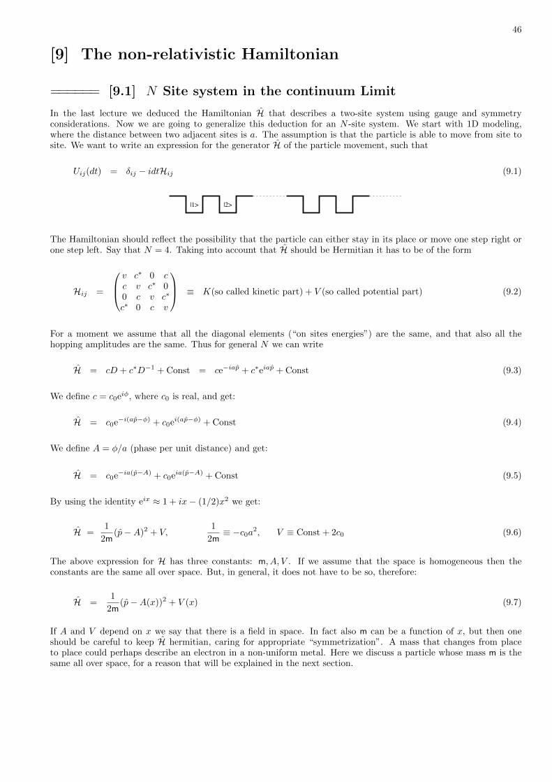
46

[9] The non-relativistic Hamiltonian

====== [9.1] N Site system in the continuum Limit

In the last lecture we deduced the Hamiltonian H that describes a two-site system using gauge and symmetryconsiderations. Now we are going to generalize this deduction for an N -site system. We start with 1D modeling,where the distance between two adjacent sites is a. The assumption is that the particle is able to move from site tosite. We want to write an expression for the generator H of the particle movement, such that

Uij(dt) = δij − idtHij (9.1)

|2>|1>

The Hamiltonian should reflect the possibility that the particle can either stay in its place or move one step right orone step left. Say that N = 4. Taking into account that H should be Hermitian it has to be of the form

Hij =

v c∗ 0 cc v c∗ 00 c v c∗

c∗ 0 c v

≡ K(so called kinetic part) + V (so called potential part) (9.2)

For a moment we assume that all the diagonal elements (“on sites energies”) are the same, and that also all thehopping amplitudes are the same. Thus for general N we can write

H = cD + c∗D−1 + Const = ce−iap + c∗eiap + Const (9.3)

We define c = c0eiφ, where c0 is real, and get:

H = c0e−i(ap−φ) + c0ei(ap−φ) + Const (9.4)

We define A = φ/a (phase per unit distance) and get:

H = c0e−ia(p−A) + c0eia(p−A) + Const (9.5)

By using the identity eix ≈ 1 + ix− (1/2)x2 we get:

H =1

2m(p−A)2 + V,

1

2m≡ −c0a2, V ≡ Const + 2c0 (9.6)

The above expression for H has three constants: m, A, V . If we assume that the space is homogeneous then theconstants are the same all over space. But, in general, it does not have to be so, therefore:

H =1

2m(p−A(x))2 + V (x) (9.7)

If A and V depend on x we say that there is a field in space. In fact also m can be a function of x, but then oneshould be careful to keep H hermitian, caring for appropriate “symmetrization”. A mass that changes from placeto place could perhaps describe an electron in a non-uniform metal. Here we discuss a particle whose mass m is thesame all over space, for a reason that will be explained in the next section.

47

====== [9.2] The Hamiltonian of a Particle in 3-D Space

In 3D we can adopt the same steps in order to deduce the Hamiltonian. We write:

H = cDx + c∗D−1x + cDy + c∗D−1

y + cDz + c∗D−1z (9.8)

= ce−iapx + c∗eiapx + ce−iapy + c∗eiapy + ce−iapz + c∗eiapz

After expanding to second order and allowing space dependence we get:

H =1

2m(px −Ax(x, y, z))2 +

1

2m(py −Ay(x, y, z))2 +

1

2m(pz −Az(x, y, z))2 + V (x, y, z)

=1

2m(p−A(r))2 + V (r) =

1

2m(p− A)2 + V (9.9)

This is the most general Hamiltonian that is invariant under Galilein transformations. Note that having a mass thatis both isotropic and position-independent is required by this invariance requirement. The Galilein group includestranslations, rotations and boosts. The relativistic version of the Galilein group is the Lorentz group (not includedin the syllabus of this course). In addition, we expect the Hamiltonian to be invariant under gauge transformations,which is indeed the case as further discussed below.

====== [9.3] Invariance of the Hamiltonian

The definition of ”invariance” is as follows: Given that H = h(x, p;V,A) is the Hamiltonian of a system in the labora-

tory reference frame, there exist V and A such that the Hamiltonian in the ”new” reference frame is H = h(x, p; V , A).The most general Hamiltonian that is invariant under translations, rotations and boosts is:

H = h(x, p;V,A) =1

2m(p−A(x))2 + V (x) (9.10)

Let us demonstrate the invariance of the Hamiltonian under translations: in the original basis |x〉 we have the fields

V (x) and A(x). In the translated reference frame the new basis is |x〉 ≡ |x+ a〉, hence 〈x|H|x′〉 = 〈x|H|x′〉 with

H = D†HD. Hence we deduce that the Hamiltonian is ”invariant” (keeps its form) with

V (x) = V (x+ a) (9.11)

A(x) = A(x+ a) (9.12)

In order to verify that we are not confused with the signs, let us consider the potential V (x) = δ(x). If we make a

translation with a = 7, then the basis in the new reference frame will be |x〉 = |x+ 7〉, and we get V (x) = δ(x+ 7)which means a delta at x = −7.

For completeness we cite how the Hamiltonian transform under Galilean transformation T to a moving frame whosevelocity is v0. This transformation is composed of a translation e−iv0tp and a boost eimv0x. The following result isderived in a dedicated lecture:

H = T †H T − v0 · p = h(x, p; V , A) (9.13)

where

V (x) = V (x+ v0t) − v0 ·A(x+ v0t) (9.14)

A(x) = A(x+ v0t) (9.15)

From here follows the well know no-relativistic transformation E = E + v0 × B, and B = B.

48

====== [9.4] The dynamical phase, electric field

Consider the case where there is no hopping between sites (c0 = 0). Accordingly the Hamiltonian H = V (x) does not

include a kinetic part, and the evolution operator is U(t) = exp[−itV (x)]. A particle that is located in a given pointin space will accumulate so called a dynamical phase:

U(t)|x0〉 = e−itV (x0)|x0〉 (9.16)

The potential V is the ”dynamical phase” that the particle accumulates per unit time. The V in a specific site iscalled ”binding energy” or ”on site energy” or ”potential energy” depending on the physical context. A V (x) thatchanges from site to site reflects the non-homogeneity of the space, or the presence of an ”external field”. To furtherclarify the significance of V let us consider a simple prototype example. Let us assume that V (x) = −Ex. If theparticle is initially prepared in a momentum eigenstate we get after some time

U(t)|p0〉 = e−itV |p0〉 = eiEtx|p0〉 = |p0 + Et〉 (9.17)

This means that the momentum changes with time. The rate of momentum increase equals E . We shall see later thatthis can be interpreted as the ”second law of Newton”.

====== [9.5] The geometric phase, magnetic field

Once we assume that the particle can move from site to site we have a hopping amplitude which we write as c = c0eiφ.It includes both a geometric phase φ and an inertial parameter c0. The latter tells us what is the tendency of theparticle to ”leak” from site to site. In order to have a Galileo invariant Hamiltonian we assume that c0 is isotropicand the same all over space, hence we can characterize the particle by its inertial mass m.

Still, in general the hopping amplitudes might be complex numbers ci→j ∝ eiφi→j . These phases do not threatenGalileo invariance. Accordingly, as the particle moves from site to site, it accumulates in each jump an additionalphase φi→j that can vary along its path. This is called ”geometric phase”. By definition the vector potential A is the”geometric phase” that the particle accumulates per unit distance. It is defined via the following formula:

φi→j ≡ ~A · (rj − ri) = Axdx+Aydy +Azdz (9.18)

The three components of ~A give the accumulated phase per distance for motion in the X, Y, and Z directionsrespectively. An infinitesimal jump in a diagonal direction is regarded as a sum of infinitesimal jumps in the X, Y,and Z directions, hence the scalar product.

In the following section we shall clarify that using gauge freedom we can describe the same system by a different ~A.

However, the circulation of ~A, which gives the total phase that is accumulated along a closed trajectory, is gaugeinvariant. Consequently we can define the circulation per unit area:

B = ∇×A (9.19)

We shall see later that this can be interpreted as ”magnetic field”. This field characterizes ~A in a gauge invariant way.

====== [9.6] What determines V (x) and A(x)

We have defined V (x) and A(x) as the phase that is accumulated by a particle per time or per distance, respectively.In the next section we shall see that the presence of V (x) and A(x) in the Hamiltonian are required in order to ensuregauge invariance: the Hamiltonian should have the same form irrespective of the way we gauge the ”phases” of theposition basis states. Next comes the physical question: what determines V (x) and A(x) in reality. A-priori theparticle can accumulate phase either due to a non-trivial geometry of space-time, or due to the presence of fields. Theformer effect is called Gravitation, while the latter are implied by the standard model. For our purpose it is enough to

49

consider the electromagnetic (EM) field. It is reasonable to postulate that different particles have different couplingsto the EM field. Hence we characterize a particle by its charge (e) and write in CGS units:

V (x) = V (x) + eV EM(x) (9.20)

A(x) = A(x) + (e/c)AEM(x) (9.21)

With regard to the gravitation we note that on the surface of Earth we have V = mgh, where h is the vertical heightof the particle, and ∇×A = 2mΩ which is responsible for the Coriolis force. Note that by the equivalence principle,so-called fictitious forces are merely a simple example of a gravitational effect, i.e. they reflect a non-trivial metrictensor that describes the space-time geometry in a given coordinate system.

From now on, unless stated otherwise, V (x) and A(x) refer to the electromagnetic field. We note that in the Feynmanpath-integral formalism, which we describe in a different lecture, the probability amplitude of a particle to get formpoint 1 to point 2, namely 〈x2|U(t2, t1)|x1〉, is expressed as a sum over amplitudes exp[iφ[x(t)]]. The sum extendsover all possible paths. The contribution of the electromagnetic field to the accumulated phase along a give path is

φ[x(t)] = φ0[x(t)] +

∫ 2

1

A · dx −∫ 2

1

V · dt (9.22)

One realizes that this is the so called ”action” in classical mechanics.

====== [9.7] Invariance under Gauge Transformation

Let us define a new basis:

|x1〉 = e−iΛ1 |x1〉 (9.23)

|x2〉 = e−iΛ2 |x2〉

and in general:

|x〉 = e−iΛ(x)|x〉 (9.24)

The hopping amplitudes in the new basis are:

c1→2 = 〈x2|H|x1〉 = ei(Λ2−Λ1)〈x2|H|x1〉 = ei(Λ2−Λ1)c1→2 (9.25)

We can rewrite this as:

φ1→2 = φ1→2 + (Λ2 − Λ1) (9.26)

Dividing by the size of the step and taking the continuum limit we get:

A(x) = A(x) +d

dxΛ(x) (9.27)

Or, in three dimensions:

A(x) = A(x) +∇Λ(x) (9.28)

We see that the Hamiltonian is invariant (keeps its form) under gauge. As we have said, there is also invariance for allthe Galilei transformations (notably boosts). This means that it is possible to find transformation laws that connectthe fields in the ”new” reference frame with the fields in the ”laboratory” reference frame.

50

====== [9.8] Is it possible to simplify the Hamiltonian further?

Is it possible to find a gauge transformation of the basis so that A will disappear? We have seen that for a two-sitesystem the answer is yes: by choosing Λ(x) correctly, we can eliminate A and simplify the Hamiltonian. On the otherhand, if there is more than one route that connects two points, the answer becomes no. The reason is that in anygauge we may choose, the following expression will always be gauge invariant:∮

A · dl =

∮A · dl = gauge invariant (9.29)

In other words: it is possible to change each of the phases separately, but the sum of phases along a closed loop willalways stay the same. We shall demonstrate this with a three-site system:

|1> |2>

|3>

|1〉 = e−iΛ1 |1〉 (9.30)

|2〉 = e−iΛ2 |2〉|3〉 = e−iΛ3 |3〉φ1→2 = φ1→2 + (Λ2 − Λ1)

φ2→3 = φ2→3 + (Λ3 − Λ2)

φ3→1 = φ3→1 + (Λ1 − Λ3)

φ1→2 + φ2→3 + φ3→1 = φ1→2 + φ2→3 + φ3→1

If the system had three sites but with an open topology, then we could have gotten rid of A like in the two-site system.That is also generally true of all the one dimensional problems, if the boundary conditions are ”zero” at infinity. Oncethe one-dimensional topology is closed (”ring” boundary conditions) such a gauge transformation cannot be made.Furthermore, when the motion is in two or three dimensional space, there is always more than one route that connectsany two points, without regard to the boundary conditions. Consequently we can define the gauge invariant field Bthat characterizes A. It follows that in general one cannot eliminate A from the Hamiltonian.

====== [9.9] Gauging away the V (x) potential

We have concluded that in general it is impossible to gauge away the A(x). But we can ask the opposite question,whether it is possible to gauge away the V (x). The answer here is trivially positive, but the ”price” is getting timedependent hopping amplitudes. Namely, the gauge transformation that does the job is

|x〉 = e−iΛ(x,t)|x〉 with Λ(x, t) = V (x) t (9.31)

This is a temporal gauge of the basis. It is analogous to a transforming into a moving frame (in both cases the newbasis is time dependent relative to the lab frame). In the new frame we have

V (x; t) = 0 (9.32)

A(x; t) = A(x) + t∇V (x) (9.33)

Hence we get the same magnetic and electric fields, but now both derived from a time dependent A(x; t).

51

[10] Getting the equations of motion

====== [10.1] Rate of change of the expectation value

Given an Hamiltonian, with any operator A we can associate an operator B,

B = i[H, A] +∂A

∂t(10.1)

such that

d〈A〉dt

= 〈B〉 (10.2)

proof: From the expectation value formula:

〈A〉t = trace(Aρ(t)) (10.3)

Using the Liouville equation and the cyclic property of the trace, we get:

d

dt〈A〉t = trace

(∂A

∂tρ(t)

)+ trace

(Adρ(t)

dt

)(10.4)

= trace

(∂A

∂tρ(t)

)− itrace (A[H, ρ(t)])

= trace

(∂A

∂tρ(t)

)+ itrace ([H, A]ρ(t))

=

⟨∂A

∂t

⟩+ i 〈[H, A]〉

Optionally, if the state is pure, we can write:

〈A〉t = 〈ψ(t)|A|ψ(t)〉 (10.5)

Using the Schrodinger equation, we get

d

dt

⟨A⟩

=⟨ ddtψ∣∣∣A∣∣∣ψ⟩+

⟨ψ∣∣∣A∣∣∣ d

dtψ⟩

+⟨ψ∣∣∣∂A∂t

∣∣∣ψ⟩ (10.6)

= i⟨ψ∣∣∣HA∣∣∣ψ⟩− i⟨ψ∣∣∣AH∣∣∣ψ⟩+

⟨ψ∣∣∣∂A∂t

∣∣∣ψ⟩ = ...

We would like to highlight the distinction between a full derivative and a partial derivative. Let us assume that thereis an operator that perhaps represents a field that depends on the time t:

A = x2 + tx8 (10.7)

Then the partial derivative with respect to t is:

∂A

∂t= x8 (10.8)

While the total derivative of 〈A〉 takes into account the change in the quantum state too.

52

====== [10.2] The classical equations of motion

If x is the location of a particle, then its rate of change is called velocity. By the rate of change formula we identifythe velocity operator v as follows:

v = i[H, x] = i

[1

2m(p−A(x))2, x

]=

1

m(p−A(x)) (10.9)

and we have:

d〈x〉dt

= 〈v〉, 3D: x := (x, y, z), v := (vx, vy, vz) (10.10)

It is useful to relaize that the kinetic part of the Hamiltonian can be written as (1/2)mv2. The commutaion relationsof the velocity components are

[mvi,mvj ] = i(∂iAj − ∂jAi) = iεijkBk (10.11)

[V (x),mvj ] = i ∂jV (x) (10.12)

The rate of change of the velocity v is called acceleration. By the rate of change formula

d〈v〉dt

=

⟨i

[1

2mv2 + V (x), v

]+∂v

∂t

⟩=

1

m

⟨1

2(v × B − B × v) + E

⟩(10.13)

Note that this is dense vector-style writing of 3 equations, for the rate of change of 〈vx〉 and 〈vy〉 and 〈vz〉. Above wehave used the follwing notations:

B = ∇×A (10.14)

E = −∂A∂t−∇V

We would like to emphasize that the Hamiltonian is the ”generator” of the evolution of the system, and therefore allthe equations of motion can be derived from it. From the above it follows that in case of a ”minimal” wavepacketthe expectation values of x and v obey the classical equations approximately. The classical Lorentz force equationbecomes exact if the B and E are constants in the region where the motion takes place:

d〈v〉dt

=1

m

[− B0 × 〈v〉+ E0

](10.15)

====== [10.3] Heuristic interpretation

In the expression for the acceleration we have two terms: the “electric” force and the “magnetic” (Lorentz) force.These forces bend the trajectory of the particle. It is important to realize that the bending of trajectories has to dowith interference and has a very intuitive heuristic explanation. This heuristic explanation is due to Huygens: Weshould regard each front of the propagating beam as a point-like source of waves. The next front (after time dt) isdetermined by interference of waves that come from all the points of the previous front. For presentation purposeit is easier to consider first the interference of N = 2 points, then to generalize to N points, and then to take thecontinuum limit of plane-wave front. The case N = 2 is formally equivalent to a two slit experiment. The mainpeak of constructive interference is in the forward direction. We want to explain why the presence of an electric or amagnetic field can shift the main peak. A straightforward generalization of the argument explains why a trajectoryof a plane-wave is bent.

53

The Huygens deflection formula: Consider a beam with wavenumber k that propagates in the x direction. Itgoes through two slits that are located on the y axis. The transverse distance between the slits is d. A detector ispositioned at some angle θ very far away from the slits. The phase difference between the oscillations that arrive tothe detector from the two slits is

φ2 − φ1 = ∆φ − k · d · θ (10.16)

In this formula it is assumed that after the slits there is a ”scattering region” of length ∆x where fields may beapplied. We define ∆φ as the phase difference after this ”scattering region”, while φ2 − φ1 is the phase difference atthe very distant detector. The ray propagation direction is defined by the requirement φ2 − φ1 = 0, leading to theoptical deflection formula θ = ∆φ/(kd). Changing notations k 7→ px and d 7→ ∆y we write the deflection formula asfollows:

θ =∆pypx

= Deflection angle (10.17)

∆py ≡ ∆φ

∆y= Optical Impulse (10.18)

From the definition of the dynamical and the geometrical phases it follows that if there are electric and magneticfields in the scattering region then

∆φ = (V2 − V1)∆t + ΦB (10.19)

where ΦB = B∆x∆y is the magnetic flux that is enclosed by the interfering rays, and V2 − V1 = E∆y is the potentialdifference between the two slits, and ∆t = ∆x/v is the travel time via the scattering region. From here follows thatthe optical impulse is

∆py =∆φ

∆y= E∆t + B∆x (10.20)

The Newtonian deflection formula: In the Newtonian perspective the deflection of a beam of particles is

θ =∆pypx

= Deflection angle (10.21)

∆py ≡ F∆t = Newtonian Impulse (10.22)

where F is called the ”Newtonian force”. By comparison with the Huygens analysis we deduce that the ”force” onthe particles is

F =∆py∆t

= E + Bv = Lorentz force (10.23)

It is important to realize that the deflection is due to an interference effect: The trajectory is bending either due toa gradient in V (x), or due to the presence of an enclosed magnetic flux. Unlike the classical point of view, it is notB(x) that matters but rather A(x), which describes the geometric accumulation of the phase along the interferingrays. We further discuss this interference under the headline “The Aharonov Bohm effect”:

54

====== [10.4] The continuity Equation (conservation of probability)

The Schrodinger equation is traditionally written as follows:

H = H(x, p) (10.24)

∂|Ψ〉∂t

= −iH|Ψ〉

∂Ψ

∂t= −iH

(x,−i ∂

∂x

)Ψ

∂Ψ

∂t= −i

[1

2m(−i∇−A(x))2 + V (x)

]Ψ(x)

Using the ”rate of change formula” for the probability density we can obtain a continuity equation:

∂ρ(x)

∂t= −∇ · J(x) (10.25)

In this formula the probability density and probability current are defined as the expectation values of the followingoperators:

ρ(x) = δ(x− x) (10.26)

J(x) =1

2(vδ(x− x) + δ(x− x)v)) (10.27)

leading to

ρ(x) = 〈Ψ|ρ(x)|Ψ〉 = |Ψ(x)|2 (10.28)

J(x) = 〈Ψ|J(x)|Ψ〉 = Re

[Ψ∗(x)

1

m(−i∇−A(x))Ψ(x)

](10.29)

The procedure to get this result can be optionally applied to a particle in an N -site system (see appropriate ”QM inpractice” section).

====== [10.5] Definition of generalized forces

We would like to know how the system energy changes when we change a parameters X on which the Hamiltonian Hdepends. We define the generalized force F as

F = −∂H∂X

(10.30)

We recall that the rate of change formula for an operator A is:

d〈A〉dt

=

⟨i[H, A] +

∂A

∂t

⟩(10.31)

In particular, the rate of change of the energy is:

dE

dt=

d〈H〉dt

=

⟨i[H, H] +

∂H∂t

⟩=

⟨∂H∂t

⟩= X

⟨∂H∂X

⟩= −X 〈F〉 (10.32)

55

If E(0) is the energy at time t = 0 we can calculate the energy E(t) at a later time. Using standard phrasing we saythat an external work E(t) − E(0) is involved in the process. Hence it is customary to define the work W which isdone by the system as:

W = −(E(t)− E(0)) =

∫〈F〉 Xdt =

∫〈F〉 dX (10.33)

A ”Newtonian force” is associated with the displacement of a piston. A generalized force called ”pressure” is associatedwith the change of the volume of a box. A generalized force called ”polarization” is associated with the change in anelectric field. A generalized force called ”magnetization” is associated with the change in a magnetic field.

====== [10.6] Definition of currents

There are two ways to define ”current” operators. The ”probability current” is defined via the rate of change of theoccupation operator (see discussion of the ”continuity equation”). The ”electrical current” is defined as the generalizedforce associated with the change in a magnetic flux, as explained below.

Let us assume that at a moment t the flux is Φ, and that at the moment t+ dt the flux is Φ + dΦ. The electromotiveforce (measured in volts) is according to Faraday’s law:

EMF = −dΦ

dt(10.34)

If the electrical current is I then the amount of charge that has been displaced is:

dQ = Idt (10.35)

The (”external”) work which is done by the electric field on the displaced charge, is

−dW = EMF× dQ = −IdΦ (10.36)

This formula implies that the generalized force which is associated with the change of magnetic flux is in fact theelectrical current. Note the analogy between flux and magnetic field, and hence between current and magnetization.In fact one can regard the current in the ring as the ”magnetization” of a spinning charge.

56

====== [10.7] The Concept of Symmetry

Pedagogical remark: In order to motivate and to clarify the abstract discussion in this section it is recommended toconsider the problem of finding the Landau levels in Hall geometry, where the system is invariant to x translations andhence px is a constant of motion. Later the ideas are extended to discuss motion in centrally symmetrical potentials.

We emphasize that symmetry and invariance are two different concepts. Invariance means that the laws of physicsand hence the form of the Hamiltonian do not change. But the fields in the Hamiltonian may change. In contrastto that in case of a symmetry we requite H = H, meaning that the fields look the literally same. As an exampleconsider a particle that moves in the periodic potential V (x;R) = cos(2π(x − R)/L). The Hamiltonian is invariantunder translations: If we make translation a then the new Hamiltonian will be the same but with R = R− a. But inthe special case that R/L is an integer we have symmetry, because then V (x;R) stays the same.

====== [10.8] What is the meaning of commutativity?

Let us assume for example that [H, px] = 0. We say in such case that the Hamiltonian commutes with the generatorof translations. What are the implication of this statement? The answer is that in such case:

• The Hamiltonian is symmetric under translations• The Hamiltonian is block diagonal in the momentum basis• The momentum is a constant of motion• There might be systematic degeneracies in the spectrum

The second statement follows from the “separation of variables” theorem. The third statement follows from theexpectation value rate of change formula:

d〈px〉dt

= 〈i[H, px]〉 = 0 (10.37)

For time independent Hamiltonians E = 〈H〉 is a constant of the motion because [H,H] = 0. Thus 〈H〉 = constis associated with symmetry with respect to “translations” in time, while 〈p〉 = const is associated with symmetrywith respect to translations in space, and 〈L〉 = const is associated with symmetry with respect to rotations. In thefollwing two subsection we further dwell on the first and last statements in the above list.

====== [10.9] Symmetry under translations and rotations

We would like to clarify the algebraic characterization of symmetry. For simplicity of presentation we considertranslations. We claim that the Hamiltonian is symmetric under translations iff

[H, pi] = 0 for i = x, y, z (10.38)

This implies that

[H, D(a)] = 0, for any a (10.39)

which can be written as HD −DH = 0, or optionally as

D−1HD = H (10.40)

If we change to a translated frame of reference, then we have a new basis which is defined as follows:

|x〉 = |x+ a〉 = D|x〉 (10.41)

The transformation matrix is

Tx1,x2 ≡ 〈x1|x2〉 =[D(a)

]x1,x2

(10.42)

57

and the Hamiltonian matrix in the new basis is

Hx1,x2≡ 〈x1|H|x2〉 =

[T−1HT

]x1,x2

(10.43)

The commutation of H with D implies that the transformed Hamiltonian H is the same in the translated frame ofreference.

An analogous statement holds for rotations. The algebraic characterization of symmetry in this case is

[H, Li] = 0 for i = x, y, z (10.44)

which implies

[H, R(~Φ)] = 0, for any ~Φ (10.45)

leading as before to the conclusion that the Hamiltonian remains the same if we transform it to a rotated frame ofreference.

====== [10.10] Symmetry implied degeneracies

Let us assume that H is symmetric under translations D. Then if |ψ〉 is an eigenstate of H then also |ϕ〉 = D|ψ〉 isan eigenstate with the same eigenvalue. This is because

H|ϕ〉 = HD|ψ〉 = DH|ψ〉 = E|ϕ〉 (10.46)

Now there are two possibilities. One possibility is that |ψ〉 is an eigenstate of D, and hence |ϕ〉 is the same state as|ψ〉. In such case we say that the symmetry of |ψ〉 is the same as of H, and a degeneracy is not implied. The otherpossibility is that |ψ〉 has lower symmetry compared with H. Then it is implied that |ψ〉 and |ϕ〉 span a subspace ofdegenerate states. If we have two symmetry operations A and B, then we might suspect that some eigenstates wouldhave both symmetries: that means both A|ψ〉 ∝ |ψ〉 and B|ψ〉 ∝ |ψ〉. If both symmetries hold for all the eigenstates,then it follows that [A,B] = 0, because both are diagonal in the same basis.

In order to argue a symmetry implied degeneracy the Hamiltonian should commute with a non-commutative group ofoperators. It is simplest to explain this statement by considering an example. Let us consider particle on a clean ring.The Hamiltonian has symmetry under translations (generated by p) and also under reflections (R). We can take thekn states as a basis. They are eigenstates of the Hamiltonian, and they are also eigenstates of p. The ground staten = 0 has the same symmetries as that of the Hamiltonian and therefore there is no implied degeneracy. But |kn〉with n 6= 0 has lower symmetry compared with H, and therefore there is an implied degeneracy with its mirror image|k−n〉. These degeneracies are unavoidable. If all the states were non-degenerated it would imply that both p and Rare diagonal in the same basis. This cannot be the case because the group of translations together with reflection isnon-commutative.

The dimension of a degenerate subspace must be equal to the dimension of a representation of the symmetry group.This is implied by the following argument: One can regardH as a mutual constant of motion for all the group operators;therefore, by the “separation of variables theorem”, it induces a block-decomposition of the group representation. Thedimensions of the blocks are the dimensions of the degenerate subspaces, and at the same time they must be compatiblewith the dimensions of the irreducible representations of the group.

Above we were discussing only the systematic degeneracies that are implied by the symmetry group of the Hamiltonian.In principle we can have also “accidental” degeneracies which are not implied by symmetries. The way to ”cook”such symmetry is as follows: pick two neighboring levels, and change some parameters in the Hamiltonian so as tomake them degenerate. It can be easily argued that in general we have to adjust 3 parameters in order to cook adegeneracy. If the system has time reversal symmetry, then the Hamiltonian can be represented by a real matrix. Insuch case it is enough to adjust 2 parameters in order to cook a degeneracy.

58

Fundamentals (part III)

[11] Group representation theory

====== [11.1] Groups

A group is a set of elements with a binary operation:

• The operation is defined by a multiplication table for τ ∗ τ ′.• There is a unique identity element 1.• Every element has an inverse element such that ττ−1 = 1• Associativity: τ ∗ (τ ′ ∗ τ ′′) = (τ ∗ τ ′) ∗ τ ′′

Commutativity does not have to be obeyed: this means that in general τ ∗ τ ′ 6= τ ′ ∗ τ .

The Galilein group is our main interst. It includes translations, rotations, and boosts. A translation is specifieduniquely by three parameters a = (a1, a2, a3). Rotations are specified by (θ, ϕ,Φ), from which Φ is constructed. Aboost is parametrized by the relative velocity u = (u1, u2, u3). A general element is any translation, rotation, boost,or any combination of them. Such a group, that has a general element that can be defined using a set of parametersis called a Lie group. The Galilein group is a Lie group with 9 parameters. The rotation group is a Lie group with3 parameters.

====== [11.2] Realization of a Group

If there are ℵ elements in a group, then the number of rows in the full multiplication table will be (ℵ9)2 = ℵ18. Themultiplication table is too big for us to construct and use. Instead we use the following strategy: each element of thegroup is regarded as a transformation over some space:

element of the group = τ = (τ1, τ2, ..., τd) (11.1)

corresponding transformation = U(τ ) (11.2)

the ”group property” = U(τ )U(τ ′) = U(τ ∗ τ ′) (11.3)

The association τ 7→ U(τ ) is called a realization. For convenience we assume that the parameterization is constructedsuch that τ = (0, 0, ..., 0) is the identity, and τ ∗ τ ∗ ...∗ τ ≡ nτ , where n is the number of repetitions. Hence U(0) = 1,and U(nτ) = U(τ)U(τ)...U(τ) = U(τ)n. For example (Φx,Φy,Φz) is good parameterization of a rotation, that hasthis property, as opposed to (θ, ϕ,Φ).

It is best to consider an example. The realization that defines the Galilein group is over the six dimensional phasespace (x,v). The realization of a translation is

τa :

x = x + av = v

(11.4)

The realization of a boost is

τu :

x = xv = v + u

(11.5)

and the realization of a rotation is

τΦ :

x = RE(Φ)xv = RE(Φ)v

(11.6)

59

A translation by b, and afterward a translation by a, gives a translation by b + a. This composition rule is simple.More generally the ”multiplication” of group elements τ = τ ′ ∗ τ ′′ implies a very complicated function

(a,Φ,u) = f(a′,Φ′,u′; a′′,Φ′′,u′′) (11.7)

We notice that this function requires 18 input parameters, and outputs 9 parameters. It is not practical to constructthis function explicitly. Rather, in order to ”multiply” elements we compose transformations.

====== [11.3] Realization using linear transformations

As mentioned above, a realization means that we regard each element of the group as an operation over a space. Wetreat the elements as transformations. Below we will discuss the possibility of finding a realization which consists oflinear transformations.

First we will discuss the concept of linear transformation, in order to clarify it. As an example, we will check whetherf(x) = x+ 5 is a linear function. A linear function must fulfill the condition:

f(αX1 + βX2) = αf(X1) + βf(X2) (11.8)

Checking f(x):

f(3) = 8, f(5) = 10, f(8) = 13 (11.9)

f(3 + 5) 6= f(3) + f(5)

Hence we realize that f(x) is not linear.

In the defining realization of the Galilein group over phase space, rotations are linear transformations, but translationsand boosts are not. If we want to realize the Galilein group using linear transformations, the most natural way wouldbe to define a realization over the function space. For example, the translation of a function is defined as:

τa : Ψ(x) = Ψ(x− a) (11.10)

The translation of a function is a linear operation. In other words, if we translate the function αΨa(x) + βΨb(x) a spa-tial distance d, then we get the appropriate linear combination of the translated functions αΨa(x− d) + βΨb(x− d).

Linear transformations are represented by matrices. This leads us to the concept of a ”representation”, which wediscuss in the next section.

====== [11.4] Representation of a group using matrices

A representation is a realization of the elements of a group using matrices. With each element τ of the group, weassociate a matrix Uij(τ ). The requirement is to have the ”multiplication table” for the matrices would be be in one-to-one correspondence to the multiplication table of the elements of the group. Below we ”soften” this requirement,being satisfied with having a ”multiplication table” that is the same ”up to a phase factor”:

U(τ ′ ∗ τ ′′) = ei(phase)U(τ ′)U(τ ′′) (11.11)

It is natural to realize the group elements using orthogonal transformations (over a real space) or unitary transforma-tions (over a complex space). Any realization using a linear transformation is automatically a ”representation”. Thereason for this is that linear transformations are always represented by matrices. For example, we may consider therealization of translations over the function space. Any function can be written as a combination of delta functions:

Ψ(x) =

∫Ψ(x′)δ(x− x′)dx (11.12)

60

In Dirac notation this can be written as:

|Ψ〉 =∑x

Ψx|x〉 (11.13)

In this basis, each translation is represented by a matrix:

Dx,x′ = 〈x|D(a)|x′〉 = δ(x− (x′ + a)) (11.14)

Finding a ”representation” for a group is very useful: the operative meaning of ”multiplying group elements” becomes”multiplying matrices”. This means that we can deal with groups using linear algebra tools.

====== [11.5] Generators

Every element in a Lie group is specified by a set of parameters. Below we assume that we have a ”unitary represen-tation” of the group. That means that there is a mapping

τ 7→ U(τ1, τ2, ...) (11.15)

We also use the convention:

1 7→ U(0, 0, ...) = 1 = identity matrix (11.16)

We define a set of generators Gµ in the following way:

U(δτ1, 0, 0, ...) = 1− iδτ1G1 = e−iδτ1G1 , [etc.] (11.17)

The number of independent generators is the same as the number of parameters that specify the elements of thegroup, e.g. 3 generators for the rotation group. In the case of the Galieli we have 9 generators, but since we allowarbitrary phase factor in the multiplaication table, we have in fact 10 generators:

Px, Py, Pz, Jx, Jy, Jz, Qx, Qy, Qz, and 1. (11.18)

Consider the standard representation over wavefunctions. It follows from the commutation relation [x, p] = i that −xis the generator of translations in p. Hence it follows that he generators of the boosts are Qx = −mx, where m is themass.

====== [11.6] Generating a representation

In general a transformation that is generated by a generator A would not commute with a transformation that isgenerated by a different generator B,

eAeB 6= eBeA 6= eA+B (11.19)

But if the generated transformations are infinitesimal then:

eε(A+B) = eεAeεB = eεBeεA = 1 + εA+ εB +O(ε2) (11.20)

If ε is not small we can still do the exponentiation in ”small steps” using the so called ”Trotter formula”, namely,

eA+B = limN→∞

[e(1/N)A e(1/N)B

]N(11.21)

61

We can use this observation in order to show that any transformation U(τ) can be generated using the completeset of generators that has been defined in the previous section. This means that it is enough to know what are thegenerators in order to calculate all the matrices of a given representation. Defining δτ = τ/N . where N is arbitrarilylarge, the calculation goes as follows:

U(τ) = [U(δτ)]N (11.22)

= [U(δτ1)U(δτ2)...]N =

= [e−iδτ1G1e−iδτ2G2 ...]N =

= [e−iδτ1G1−iδτ2G2...]N =

= [e−iδτ ·G]N = e−iτ ·G

In the above manipulation infinitesimal transformations are involved, hence it was allowed to perform O(N) transpo-sitions in the ordering of their multiplication. Obviously the number of transpositions should not reach O(N2), elsethe accumulated error would invalidate the procedure. The next issue is how to multiply transformations. For thiswe have to learn about the algebra of the generators.

====== [11.7] Combining generators

It should be clear that if A and B generate (say) rotations, it does not imply that (say) the hermitian operatorAB +BA is a generator of a rotation. On the other hand we have the following important statement: if A and B aregenerators of group elements, then also G = αA+ βB and G = i[A,B] are generators of group elements.

Proof: By definition G is a generator if e−iεG is a matrix that represents an element in the group. We will prove thestatement by showing that the infinitesimal transformation e−iεG can be written as a multiplication of matrices thatrepresent elements in the group. In the first case:

e−iε(αA+βB) = e−iεαA e−iεβB (11.23)

In the second case we use the identity:

eε[A,B] = e−i√εB e−i

√εA ei

√εB ei

√εA + O(ε2) (11.24)

This identity can be proved as follows:

1 + ε(AB −BA) = (1− i√εB − 1

2εB2)(1− i

√εA− 1

2εA2)(1 + i

√εB − 1

2εB2)(1 + i

√εA− 1

2εA2) (11.25)

====== [11.8] Structure constants

Any element in the group can be written using the set of basic generators:

U(τ) = e−iτ ·G (11.26)

From the previous section it follows that i[Gµ, Gν ] is a generator. Therefore, it must be a linear combination of thebasic generators. In other words, there exit constants cλµν such that the following closure relation is satisfied:

[Gµ, Gν ] = i∑λ

cλµνGλ (11.27)

62

The constants cλµν are called the ”structure constants” of the group. Every ”Lie group” has its own structurecoefficients. If we know the structure constants, we can reconstruct the group ”multiplication table”. In the nextlecture we shall deduce the structure constants of the rotation group from its defining representation, and then weshall learn how to build up all its other representations, just from our knowledge of the structure constants.

====== [11.9] The structure constants and the multiplication table

In order to find the group multiplication table based on our knowledge of the generators, we can use, in principle, thefollowing formula:

eAeB = eA+B+C (11.28)

Here C is an expression that includes only commutators. There is no simple expression for C. However, it is possibleto find an explicit expression up to any desired accuracy. This is called the Baker-Campbell-Hausdorff formula. ByTaylor expansion up to the third order we deduce:

C = log(eAeB)−A−B =1

2[A,B] +

1

12[(A−B), [A,B]] + ... (11.29)

From this we conclude that:

e−iα·G−iβ·G = e−iγ·G (11.30)

where

γλ = αλ + βλ +1

2cλµναµβν −

1

12cλκσc

κµν(α− β)σαµβν + ... (11.31)

For more details see Wikipedia, or a paper by Wilcox (1967) that is available in the course site.

====== [11.10] The group of rotations

In the next lecture we are going to concentrate of the group of rotations. More precisely we consider on equalfooting the groups SO(3) and SU(2). Both a characterized by the same Lie algebra, and consequently share the samemultiplication table up to phase factors.

====== [11.11] The Heisenberg group

In the present section we relate to the group of translations and boosts. Without loss of generality we assume aone-dimensional geometrical space. One option is to define this group is via a realization over an (x, v) phase space. Ifwe adopt this definition we get a Abelian group whose elements commute with each other. Let us call it the ”Galileinversion” of the group.

Optionally we can consider a realization of translations and boosts over complex wavefunctions Ψ(x). In the standardrepresentation the space of wavefunctions is spanned by the eigenstates of the x operator, and the translations aregenerated by P = p. It follows from [x, p] = i that the generator of boosts is Q = −x. Hence the group is non-Abelianand characterized by the Lie algebra [P,Q] = i. It is known as the ”Heisenberg group”. It has the same multiplicationtable as the Abelian ”Galilein version”, up to phase factors.

If we believe (following the two slit experiment) that the state of particle is described by a wavefunction, it follows,as argued above, that boost and translations do not commute. Let us illuminate this point using an intuitive physicslanguage. Say we have a particle in the laboratory reference frame that is described by a wavefunction Ψ(x) that isan eigenstate of the translation operators. In other words, we are talking about a momentum eigenstate that has awell defined wavenumber k. Let us transform to a moving reference frame. Assuming that boosts were commuting

63

with translations, if follows that boost is a symmetry operation, and hence the transformed state Ψ(x) is still amomentum eigenstate with the same k. From this we would come to the absurd conclusion that the particle has thesame momentum in all reference frames.

It is interesting to look for a realization of the Heisenberg group over a finite-dimensional ”phase-space”. For thispurpose we have to assume that phase space has a third coordinate: instead of (x, v) we need (a, b, c). The way tocome to this conclusion is based on the observation that any element of the Heisenberg group can be written in thestandard representation as

U(a, b, c) = exp (iaQ+ ibP + ic) (11.32)

Hence the multiplication U(a1, b1, c1)U(a2, b2, cc) is realized by the composition law

(a1, b1, c1

)?(a2, b2, c2

)=

(a1 + a2, b1 + b2, c1 + c2,+

1

2(a1b2 − b1a2)

)(11.33)

Here a is position displacement, and b is momentum displacement, and c is an additional coordinate. If the orderof a translation and a boost is reversed the new result is different by a phase factor exp(iC), where C equals thesymplectic area of the encircled phase-space cell. This non-commutativity is reflected in the c coordinate.

64

[12] The group of rotations

====== [12.1] The rotation group SO(3)

The rotation group SO(3) is a non-commutative group. That means that the order of rotations is important. Despitethis, it is important to remember that infinitesimal rotations commute. We have already proved this statement ingeneral, but we shall prove it once again for the specific case of rotations:

R(δΦ)r = r + δΦ× r (12.1)

Therefore

R(δΦ2)R(δΦ1)r = (r + δΦ1 × r) + δΦ2 × (r + δΦ1 × r) = (12.2)

= r + (δΦ1 + δΦ2)× r =

= R(δΦ1)R(δΦ2)r

Obviously, this is not correct for finite non-infinitesimal rotations:

R(~Φ1)R(~Φ2) 6= R(~Φ1 + ~Φ2) 6= R(~Φ2)R(~Φ1) (12.3)

We can construct any infinitesimal rotation from small rotations around the major axes:

R(δ~Φ) = R(δΦx~ex + δΦy~ey + δΦz~ez) = R(δΦx~ex)R(δΦy~ey)R(δΦz~ez) (12.4)

Using the vector notation ~M = (Mx,My,Mz), we conclude that a finite rotation around any axis can be written as:

R(Φ~n) = R(~Φ) = R(δ~Φ)N = (R(δΦx)R(δΦy)R(δΦz))N (12.5)

= (e−iδ~Φ· ~M )N = e−i

~Φ· ~M = e−iΦMn

Hence we conclude that Mn = ~n · ~M is the generator of the rotations around the axis ~n.

====== [12.2] Structure constants of the rotation group

We would like to find the structure constants of the rotation group SO(3), using its defining representation. The SO(3)matrices induce rotations without performing reflections and all their elements are real. The matrix representation ofa rotation around the z axis is:

R(Φ~ez) =

cos(Φ) − sin(Φ) 0sin(Φ) cos(Φ) 0

0 0 1

(12.6)

For a small rotation:

R(δΦ~ez) =

1 −δΦ 0δΦ 1 00 0 1

= 1 + δΦ

0 −1 01 0 00 0 0

= 1− iδΦMz (12.7)

where:

Mz =

0 −i 0i 0 00 0 0

(12.8)

65

We can find the other generators in the same way:

Mx =

0 0 00 0 −i0 i 0

, My =

0 0 i0 0 0−i 0 0

(12.9)

In compact notation the 3 generators are[Mk

]ij

= −iεijk (12.10)

Now we can calculate the structure constants. For example [Mx,My] = iMz, and in general:

[Mi,Mj ] = iεijkMk (12.11)

We could of course use a different representation of the rotation group in order to deduce this Lie algebra. In particularwe could use the differential representation of the Li over the infinite-dimensional Hilbert space of wavefunctions.

====== [12.3] Motivation for finding dim=2 representation

We have defined the rotation group by the Euclidean realization over 3D space. Obviously, this representation canbe used to make calculations (”to multiply rotations”). The advantage is that it is intuitive, and there is no needfor complex numbers. The disadvantage is that they are 3 × 3 matrices with inconvenient algebraic properties, so acalculation could take hours. It would be convenient if we could ”multiply rotations” with simple 2× 2 matrices. Inother words, we are interested in a dim=2 representation of the rotation group. The mission is to find three simple2× 2 matrices that fulfill:

[Jx, Jy] = iJz etc. (12.12)

In the next lecture we will learn a systematic approach to building all the representations of the rotation group. Inthe present lecture, we will simply find the requested representation by guessing. It is easy to verify that the matrices

Sx =1

2σx, Sy =

1

2σy, Sz =

1

2σz (12.13)

fulfill the above commutation relations. So, we can use them to create a dim=2 representation of the rotation group.We construct the rotation matrices using the formula:

R = e−i~Φ·~S (12.14)

The matrices that are generated necessarily satisfy the group multiplication table.

We should remember the distinction between a realization and a representation: in a realization it matters what weare rotating. In a representation it only matters to us that the correct multiplication table is fulfilled. Is it possibleto regard any representation as a realization? Is it possible to say what the rotation matrices rotate? When there is adim=3 Euclidean rotation matrix we can use it on real vectors that represent points in space. If the matrix operateson complex vectors, then we must look for another interpretation for the vectors. This will lead us to the definitionof the concept of spin (spin 1). When we are talking about a dim=2 representation it is possible to give the vectorsan interpretation. The interpretation will be another type of spin (spin 1/2).

====== [12.4] How to calculate a general rotation matrix

The calculation of a 2× 2 rotation matrix is extremely simple. All the even powers of a given Pauli matrix are equalto the identity matrix, while all the odd powers are equal to the original matrix. From this (using Taylor expansion

66

and separating into two partial sums), we get the result:

R(Φ) = R(Φ~n) = e−iΦSn = cos(Φ/2)1− i sin(Φ/2)σn (12.15)

where σn = ~n · ~σ, and Sn = (1/2)σn is the generator of a rotation around the ~n axis.

The analogous formula for constructing a 3× 3 rotation matrix is:

R(~Φ) = R(Φ~n) = e−iΦMn = 1− (1− cos(Φ))M2n − i sin(Φ)Mn (12.16)

where Mn = ~n · ~M is the generator of a rotation around the ~n axis. The proof is based on a Taylor expansion.We notice that M3

z = Mz, from this it follows that for all the odd powers Mkz = Mz, while for all the even powers

Mkz = M2

z where k > 0. The same properties apply to any Mn, because all the rotations are ”similar” one to theother (moving to another reference frame is done by means of a similarity transformation that represents a change ofbasis).

====== [12.5] An example for multiplication of rotations

Let us make a 90o rotation R(900ez) around the Z axis, followed by a 90o rotation R(900ey) around the Y axis. Wewould like to know what this sequence gives. Using the Euclidean representation

R = 1− i sin ΦMn − (1− cos Φ)M2n (12.17)

we get

R(900ez) = 1− iMz −M2z (12.18)

R(900ey) = 1− iMy −M2y

We do not wish to open the parentheses, and add up 9 terms which include multiplications of 3× 3 matrices. Thereforewe abandon the Euclidean representation and try and do the same thing with a dim=2 representation, working withthe 2× 2 Pauli matrices.

R(Φ) = cos(Φ/2)1− i sin(Φ/2)σn (12.19)

R(900ez) =1√2

(1− iσz)

R(900ey) =1√2

(1− iσy)

Hence

R = R(900ey)R(900ez) =1

2(1− iσx − iσy − iσz) (12.20)

where we have used the fact that σyσz = iσx. We can write this result as:

R = cos120o

2− i sin

120o

2~n · ~σ (12.21)

where n = 1√3(1, 1, 1). This defines the equivalent rotation which is obtained by combining the two 90o rotations.

67

[13] Building the representations of rotations

====== [13.1] Irreducible representations

A reducible representation is a representation for which a basis can be found such that each matrix in the groupdecomposes into the same block structure. In this basis the set of single-block sub-matrices obeys the same multipli-cation table as that of the full matrices, hence we say that the representation is the sum of smaller representations.For a commutative group a basis can be found in which all the matrices are diagonal. In the latter case we can saythat the representation decomposes into one-dimensional representations.

The rotation group is not a commutative group. We are interested in finding all its irreducible representations. Letus assume that someone hands us an irreducible representation. We can find its generators, written as matrices insome ”standard basis”, and we can verify that they satisfy the desired Lie algebra. We shall see that it is enoughto know the dimension of the irreducible representation in order to figure out what are the matrices that we have inhand (up to a choice of basis). In this way we establish that there is one, and only one, irreducible representation foreach dimension.

====== [13.2] First Stage - determination of basis

If we have a representation of the rotation group, we can look at infinitesimal rotations and define generators. For asmall rotation around the X axis, we can write:

R(δΦ~ex) = 1− iδΦJx (13.1)

In the same way we can write rotations round the Z and Y axes. So, we can find the matrices Jx, Jy, Jz. How canwe check that the representation that we have is indeed a representation of the rotation group? All we have to do ischeck that the following equation is obeyed:

[Ji, Jj ] = iεijkJk (13.2)

We define:

J± = Jx ± iJy (13.3)

J2 = J2x + J2

y + J2z =

1

2(J+J− + J−J+) + J2

z

We notice that the operator J2 commutes with all the generators, and therefore also with all the rotation matrices.From the “separation of variable” theorems it follows that if J2 has (say) two different eigenvalues, then it induces adecomposition of all the rotation matrices into two blocks. So in such case the representation is reducible. Withoutloss of generality our interest is focused on irreducible representations for which we necessarily have J2 = λ1, where λis a constant. Later we shall argue that λ is uniquely determined by the dimension of the irreducible representation.

If we have a representation, we still have the freedom to decide in which basis to write it. Without loss of generality,we can decide on a basis that is determined by the operator Jz:

Jz|m〉 = m|m〉 (13.4)

Obviously, the other generators, or a general rotation matrix will not be diagonal in this basis, so we have

〈m|J2|m′〉 = λδmm′ (13.5)

〈m|Jz|m′〉 = mδmm′

〈m|R|m′〉 = Rλmm′

68

====== [13.3] Reminder: Ladder Operators

Given an operator D, which does not have to be unitary or Hermitian, and an observable x that obeys the commutationrelation

[x, D] = aD (13.6)

we prove that D is a “ladder” operator that shifts between eigenstates of x.

xD − Dx = aD (13.7)

xD = D(x+ a)

xD|x〉 = D(x+ a)|x〉xD|x〉 = D(x+ a)|x〉x[D|x〉] = (x+ a)[D|x〉]

So the state |Ψ〉 = D|x〉 is an eigenstate of x with eigenvalue (x+ a). The normalization of |Ψ〉 is determined by:

||Ψ|| =√〈Ψ|Ψ〉 =

√〈x|D†D|x〉 (13.8)

====== [13.4] Second stage: identification of ladder operators

It follows from the commutation relations of the generators that:

[Jz, J±] = ±J± (13.9)

So J± are ladder operators in the basis that we have chosen. Using them we can shift from a given eigenstate |m〉 toother eigenstates: ..., |m− 2〉, |m− 1〉, |m+ 1〉, |m+ 2〉, |m+ 3〉, ....

From the commutation relations of the generators

(J+J−)− (J−J+) = [J+, J−] = 2Jz (13.10)

From the definition of J2

(J+J−) + (J−J+) = 2(J2 − (Jz)2) (13.11)

By adding and subtracting these two identities we get respectively:

J−J+ = J2 − Jz(Jz + 1) (13.12)

J+J− = J2 − Jz(Jz − 1)

Now we can find the normalization of the states that are found by using the ladder operators:

||J+|m〉||2 = 〈m|J−J+|m〉 = 〈m|J2|m〉 − 〈m|Jz(Jz + 1)|m〉 = λ−m(m+ 1) (13.13)

||J−|m〉||2 = 〈m|J+J−|m〉 = 〈m|J2|m〉 − 〈m|Jz(Jz − 1)|m〉 = λ−m(m− 1) (13.14)

69

It will be convenient from now on to write the eigenvalue of J2 as λ = j(j + 1). Therefore:

J+|m〉 =√j(j + 1)−m(m+ 1) |m+ 1〉 (13.15)

J−|m〉 =√j(j + 1)−m(m− 1) |m− 1〉 (13.16)

====== [13.5] Third stage - deducing the representation

Since the representation is of a finite dimension, the shift process of raising or lowering cannot go on forever. Bylooking at the results of the last section we may conclude that there is only one way that the raising process couldstop: at some stage we should get m = +j. Similarly, there is only one way that the lowering process could stop: atsome stage we should get m = −j. Hence from the raising/lowering process we get a ladder that includes dim = 2j + 1basis states. This number must be an integer number. Therefore j must be either an integer or half integer number.

For a given j the matrix representation of the generators is determined uniquely. This is based on the formulas of theprevious section, from which we conclude:

[J+]m′m =√j(j + 1)−m(m+ 1) δm′,m+1 (13.17)

[J−]m′m =√j(j + 1)−m(m− 1) δm′,m−1

And all that is left to do is to write:

[Jx]m′m =1

2

[(J+)m′m + (J−)m′m

](13.18)

[Jy]m′m =1

2i

[(J+)m′m − (J−)m′m

][Jz]m′m = m δm′m

And then we get every rotation matrix in the representation by:

Rm′m = e−i~Φ· ~J (13.19)

A technical note: In the raising/lowering process described above we get a ”multiplet” of m states. Can we getseveral independent multiplets? Without loss of generality we had assumed that we are dealing with an irreduciblerepresentation, and therefore there is only one multiplet.

70

[14] Rotations of spins and of wavefunctions

====== [14.1] Building the dim=2 representation (spin 1/2)

Let us find the j = 1/2 representation. This representation can be interpreted as a realization of spin 1/2. Wetherefore we use from now on the notation S instead on J .

S2|m〉 =1

2

(1

2+ 1

)|m〉 (14.1)

Sz =

(12 00 − 1

2

)(14.2)

Using formulas of the previous section we find S+ and S− and hence Sx and Sy

S+ =

(0 10 0

)(14.3)

S− =

(0 01 0

)(14.4)

Sx =1

2

((0 10 0

)+

(0 01 0

))=

1

2σx (14.5)

Sy =1

2i

((0 10 0

)−(

0 01 0

))=

1

2σy (14.6)

We recall that

R(Φ) = R(Φ~n) = e−iΦSn = cos(Φ/2)1− i sin(Φ/2)σn (14.7)

where

~n = (sin θ cosϕ, sin θ sinϕ, cos θ) (14.8)

σn = ~n · ~σ =

(cos θ e−iϕ sin θ

eiϕ sin θ − cos θ

)(14.9)

Hence

R(~Φ) =

(cos(Φ/2)− i cos(θ) sin(Φ/2) −ie−iϕ sin(θ) sin(Φ/2)−ieiϕ sin(θ) sin(Φ/2) cos(Φ/2) + i cos(θ) sin(Φ/2)

)(14.10)

In particular a rotation around the Z axis is given by:

R = e−iΦSz =

(e−iΦ/2 0

0 eiΦ/2

)(14.11)

And a rotation round the Y axis is given by:

R = e−iΦSy =

(cos(Φ/2) − sin(Φ/2)sin(Φ/2) cos(Φ/2)

)(14.12)

71

====== [14.2] Polarization states of Spin 1/2

We now discuss the physical interpretation of the ”states” that the s = 1/2 matrices rotate. Any state of ”spin 1/2” isrepresented by a vector with two complex number. That means we have 4 parameters. After gauge and normalization,we are left with 2 physical parameters which can be associated with the polarization direction (θ, ϕ). Thus it makessense to represent the state of spin 1/2 by an arrow that points to some direction in space.

The eigenstates of Sz do not change when we rotate them around the Z axis (aside from a phase factor). Thereforethe following interpretation comes to mind:

∣∣∣∣m = +1

2

⟩= |~z〉 = | ↑〉 7→

(10

)(14.13)∣∣∣∣m = −1

2

⟩= |←z 〉 = | ↓〉 7→

(01

)(14.14)

This interpretation is confirmed by rotating the ”up” state by 180 degrees, and getting the ”down” state.

R = e−iπSy =

(0 −11 0

)(14.15)

We see that:(10

); 1800 ;

(01

); 1800 ; −

(10

)(14.16)

With two rotations of 180o we get back the ”up” state, with a minus sign. Optionally one observes that

e−i2πSz = e−iπσz = −1 (14.17)

and hence by similarity this holds for any 2π rotation. We see that the representation that we found is not a one-to-one representation of the rotation group. It does not obey the multiplication table in a one-to-one fashion! In fact,we have found a representation of SU(2) and not SO(3). The minus sign has a physical significance. In a two slitexperiment it is possible to turn destructive interference into constructive interference by placing a magnetic field inone of the paths. The magnetic field rotates the spin of the electrons. If we induce 360o rotation, then the relativephase of the interference change sign, and hence constructive interference becomes destructive and vice versa. Therelative phase is important! Therefore, we must not ignore the minus sign.

It is important to emphasize that the physical degree of freedom that is called ”spin 1/2” cannot be visualized as aarising from the spinning of small rigid body around some axis like a top. If it were possible, then we could say thatthe spin can be described by a wave function. In this case, if we would rotate it by 360o we would get the same state,with the same sign. But in the representation we are discussing we get minus the same state. That is in contradictionwith the definition of a (wave) function as a single valued object.

We can get from the ”up” state all the other possible states merely by using the appropriate rotation matrix. Inparticular we can get any spin polarization state by combining a rotation round the Y axis and a rotation round theZ axis. The result is:

|~nθ,ϕ〉 = R(ϕ)R(θ)| ↑〉 = e−iϕSze−iθSy | ↑〉 7→(

e−iϕ/2 cos(θ/2)eiϕ/2 sin(θ/2)

)(14.18)

72

====== [14.3] Building the dim=3 representation (spin 1)

Let us find the j = 1 representation. This representation can be interpreted as a realization of spin 1, and hence weuse the notation S instead of J as in the previous section.

S2|m〉 = 1(1 + 1)|m〉 (14.19)

Sz =

1 0 00 0 00 0 −1

(14.20)

S+ =

0√

2 0

0 0√

20 0 0

(14.21)

The standard representation of the generators is:

S →

1√2

0 1 01 0 10 1 0

,1√2

0 −i 0i 0 −i0 i 0

,

1 0 00 0 00 0 −1

(14.22)

We remember that the Euclidean representation is:

M →

0 0 00 0 −i0 i 0

,

0 0 i0 0 0−i 0 0

,

0 −i 0i 0 00 0 0

(14.23)

Now we have two different dim=3 representations that represent the rotation group. They are actually the samerepresentation in a different basis. By changing bases (diagonalizing Mz) it is possible to move from the Euclideanrepresentation to the standard representation. It is obvious that diagonalizing Mz is only possible over the complexfield. In the defining realization, the matrices of the Euclidean representation rotate points in the real space. But itis possible also to use them on complex vectors. In the latter case it is a realization for spin 1.

For future use we list some useful matrices:

S2x =

1

2

1 0 10 2 01 0 1

, S2y =

1

2

1 0 −10 2 0−1 0 1

, S2z =

1 0 00 0 00 0 1

(14.24)

As expected for the s = 1 representation we have

S2 = S2x + S2

y + S2z =

2 0 00 2 00 0 2

= s(s+ 1)δm,m′ (14.25)

We note that one can define a projector P z = 1− S2z on the m = 0 state. Similarly we can define projectors

P x = 1− S2x and P y = 1− S2

y . We see that this set is complete P x + P y + P z = 1, and one can verify that theseprojectors are orthogonal. In the next section we shall see that they define the Euclidean basis that consist of so-calledlinearly polarized states. In this basis the generators are represented by the matrices Mx,My,Mz.

Having found the generators we can construct any rotation of spin 1. We notice the following equation:

S3i = S2

i Si = Si for i = x, y, z (14.26)

From this equation we conclude that all the odd powers (1, 3, 5, ...) are the same and are equal to Si, and all the evenpowers (2, 4, 6, ...) are the same and equal to S2

i . It follows (by way of a Taylor expansion) that:

U(~Φ) = e−i~Φ·~S = 1− i sin(Φ)Sn − (1− cos(Φ))S2

n (14.27)

73

where:

Sn = ~n · ~S (14.28)

Any rotation can be given by a combination of a rotation round the z axis and a rotation round the y axis. We markthe rotation angle around the y axis by θ, and the rotation angle around the z axis by ϕ, and get:

U(ϕ~nz) = e−iϕSz =

e−iϕ 0 00 1 00 0 eiϕ

(14.29)

U(θ~ny) = e−iθSy =

12 (1 + cos θ) − 1√

2sin θ 1

2 (1− cos θ)1√2

sin θ cos θ − 1√2

sin θ12 (1− cos θ) 1√

2sin θ 1

2 (1 + cos θ)

(14.30)

====== [14.4] Polarization states of a spin 1

The states of ”Spin 1” cannot be represented by simple arrows. This should be obvious in advance because it isrepresented by a vector that has three complex components. That means we have 6 parameters. After gauge andnormalization, we still have 4 physical parameters. Hence it is not possible to find all the possible states of spin 1 byusing only rotations. Below we further discuss the physical interpretation of spin 1 states. This discussion suggest touse the following notations for the basis states of the standard representation:

|m = 1〉 = |~z〉 = | ⇑〉 7→

100

(14.31)

|m = 0〉 = |↔z 〉 = | m〉 7→

010

(14.32)

|m = −1〉 = |←z 〉 = | ⇓〉 7→

001

(14.33)

The first and the last states represent circular polarizations. By rotating the first state by 180o around the Y axiswe get the third state. This means that we have 180o degree orthogonality. However, the middle state is different: itdescribes linear polarization. Rotating the middle state by 180o degrees around the Y axis gives the same state again!This explains the reason for marking this state with a double headed arrow.

If we rotate the linear polarization state | m〉 by 90o, once around the Y axis and once around the X axis, we get anorthogonal set of states:

|↔x〉 =1√2

(−| ⇑〉+ | ⇓〉) 7→ 1√2

−101

(14.34)

|↔y 〉 =i√2

(| ⇑〉+ | ⇓〉) 7→ 1√2

i0i

(14.35)

|↔z 〉 = | m〉 7→

010

(14.36)

This basis is called the linear basis. States of ”spin 1” can be written either in the standard basis or in the basis

74

of linear polarizations. The latter option, where we have 90o orthogonality of the basis vectors, corresponds to theEuclidean representation.

We can rotate the state | ⇑〉 in order to get other circularly polarized states:

|~nθ,ϕ〉 = U(ϕ~nz)U(θ~ny)| ⇑〉 =

12 (1 + cos θ)e−iϕ

1√2

sin θ12 (1− cos θ)eiϕ

(14.37)

Similarly, we can rotate the state | m〉 in order to get other linearly polarized states:

|↔nθ,ϕ〉 = U(ϕ~nz)U(θ~ny)| m〉 =

− 1√2

sin θe−iϕ

cos θ1√2

sin θeiϕ

(14.38)

In particular we note that linearly polarized states in the XY plane can be written as follows:

|↔nϕ〉 =1√2

(−e−iϕ| ⇑〉+ eiϕ| ⇓〉) = cos(ϕ)|↔x〉+ sin(ϕ)|↔y 〉 (14.39)

As defined above the circularly polarized states are obtained by rotating the | ⇑〉 state, while the linearly polarizedstates are obtained by rotating the | m〉 state. But a general polarization state will not necessarily be circularlypolarized, neither linearly polarized. We shall argue below that any polarization state of spin 1 can be obtained byrotation of so-called elliptically polarized state

|elliptic〉 ≡ 1√2

(√1 + q| ⇑〉 −

√1− q| ⇓〉

)(14.40)

where 0 < q < 1. This is an interpolation between q = 1 circular polarization in the Z direction, and q = 0 linearpolarization in the X direction. The states that are obtained by rotation of the q = 1 state are the circularly polarizedstates, while the states that are obtained by rotation of the q = 0 state are the linearly polarized states. From thisfollows that a general spin 1 state is characterized by 4 parameters: q and the 3 angles that define rotation. This isconsistent with the discussion in the opening of this section.

In order to establish that the most general polarization state is elliptic we define the following procedure. Givenan arbitrary state vector (ψ+, ψ0, ψ−) we can re-orient the z axis in a (θ, ϕ) direction such that ψ0 = 0. We saythat this (θ, ϕ) direction defines a “polarization plane”. Using φ rotation around the new Z axis, and taking gaugefreedom into account, we can arrange that the amplitudes (ψ+, ψ−) would be real with opposite sign (representingX polarization). Hence we have establish that after suitable rotation we get what we called elliptic polarization thatcan be characterized by a number 0 < q < 1. Thus we see that indeed an arbitrary state is characterized by the fourparameters (θ, ϕ, φ, q). We can represent the state by an ellipse as follows: The angles (θ, ϕ) define the plane of theellipse, while φ describes the angle of major axes in this plane, and q describes the ratio of the major radii. Note that180o rotation in the polarization plane leads to the same state (with minus sign). The special case q = 0 is calledcircular polarization because any rotation in the polarization plane leads to the same state (up to a phase). Thespecial case q = 0 is called linear polarization: the ellipse becomes a double headed arrow.

It follows from the above procedure that is possible to find one-to-one relation between polarization states of spin 1and ellipses. The direction of the polarization is the orientation of the ellipse. When the ellipse is a circle, the spin iscircularly polarized, and when the ellipse shrinks down to a line, the spin is linearly polarized. In the latter case theorientation of the polarization plane is ill defined.

75

====== [14.5] Translations and rotations of wavefunctions

We first consider in this section the space of functions that live on a torus (bagel). We shall see that the representationof translations over this space decomposes into one-dimensional irreducible representations, as expected in the case ofa commutative group. Then we consider the space of functions that live on the surface of a sphere. We shall see thatthe representation of rotations over this space decomposes as 1⊕ 3⊕ 5⊕ . . .. The basis in which this decompositionbecomes apparent consists of the spherical harmonics.

Consider the space of functions that live on a torus (bagel). This functions can represent the motion of a particle in a2-D box of size Lx × Ly with periodic boundary conditions. Without loss of generality we assume that the dimensionsof the surface are Lx = Ly = 2π, and use x = (θ, ϕ) as the coordinates. The representation of the state of a particlein the standard basis is:

|Ψ〉 =∑θ,ϕ

ψ(θ, ϕ)|θ, ϕ〉 (14.41)

The momentum states are labeled as k = (n,m). The representation of a wavefunction in this basis is:

|Ψ〉 =∑n,m

Ψn,m|n,m〉 (14.42)

where the transformation matrix is:

〈θ, ϕ|n,m〉 =1

2πei(nθ+mϕ) (14.43)

The displacement operators in the standard basis are not diagonal:

Dx,x′ = δ(θ − (θ′ + a))δ(ϕ− (ϕ′ + b)) (14.44)

However, in the momentum basis we get diagonal matrices:

Dk,k′ = δn,n′δm,m′ e−i(an+bm) (14.45)

In other words, we have decomposed the translations group into 1-D representations. This is possible because thegroup is commutative. If a group is not commutative it is not possible to find a basis in which all the matrices of thegroup are diagonal simultaneously.

Now we consider the space of functions that live on the surface of a sphere. This functions can represent the motionof a particle in a 2-D spherical shell. Without loss of generality we assume that the radius of the sphere is unity. Infull analogy with the case of a torus, the standard representation of the states of a particle that moves on the surfaceof a sphere is:

|Ψ〉 =∑θ,ϕ

ψ(θ, ϕ)|θ, ϕ〉 (14.46)

Alternatively, we can work with a different basis:

|Ψ〉 =∑`m

Ψ`m|`,m〉 (14.47)

where the transformation matrix is:

〈θ, ϕ|`,m〉 = Y `m(θ, ϕ) (14.48)

76

The ”displacement” matrices are actually ”rotation” matrices. They are not diagonal in the standard basis:

Rx,x′ = δ(θ − f(θ′, ϕ′))δ(ϕ− g(θ′, ϕ′)) (14.49)

where f() and g() are complicated functions. But if we take Y `m(θ, ϕ) to be the spherical harmonics then in the newbasis the representation of rotations becomes simpler:

R`m,`′m′ =

1× 1 0 0 00 3× 3 0 00 0 5× 5 00 0 0 . . .

= block diagonal (14.50)

When we rotate a function, each block stays ”within itself”. The rotation does not mix states that have different `. Inother words: in the basis |`,m〉 the representation of rotations decomposes into a sum of irreducible representationsof finite dimension:

1⊕ 3⊕ 5⊕ . . . (14.51)

In the next section we show how the general procedure that we have learned for decomposing representations, doesindeed help us to find the Y `m(θ, ϕ) functions.

====== [14.6] The spherical harmonics

We have already found the representation of the generators of rotations over the 3D space of wavefunctions. Namely

we have proved that ~L = ~r × ~p. If we write the differential representation of L is spherical coordinates we find asexpected that the radial coordinate r is not involved:

Lz → −i ∂∂ϕ

(14.52)

L± → e±iϕ(± ∂

∂θ+ i cot(θ)

∂

∂ϕ

)(14.53)

L2 → −[

1

sin(θ)

∂

∂θ(sin(θ)

∂

∂θ) +

1

sin2 θ

∂2

∂ϕ2

](14.54)

Thus the representation trivially decompose with respect to r, and without loss of generality we can focus on thesubspace of wavefunctions Ψ(θ, ϕ) that live on a spherical shell of a given radius. We would like to find the basis inwhich the representation decomposes, as defined by

L2Ψ = `(`+ 1)Ψ (14.55)

LzΨ = mΨ (14.56)

The solution is:

Y `m(θ, φ) =

[2`+ 1

4π

(`−m)!

(`+m)!

]1/2

[(−1)mP`m(cos(θ))] eimϕ (14.57)

It is customary in quantum textbooks to absorb the factor (−1)m in the definition of the Legendre polynomials. Wenote that it is convenient to start with

Y ``(θ, φ) ∝ (sin(θ))` ei`ϕ (14.58)

77

and then to find the rest of the functions using the lowering operator:

|`,m〉 ∝ L(`−m)− |`, `〉 (14.59)

Let us give some examples for Spherical Functions. The simplest function is spread uniformly over the surface of thesphere, while a linear polarization state along the Z axis is concentrated mostly at the poles:

Y 0,0 =1√4π, Y 1,0 =

√3

4πcos(θ) (14.60)

If we rotate the polar wave function by 90 degrees we get:

Y 1,x =

√3

4πsin(θ) cos(ϕ), Y 1,y =

√3

4πsin(θ) sin(ϕ) (14.61)

While according to the standard ”recipe” the circular polarizations are:

Y 1,1 = −√

3

8πsin(θ)eiϕ, Y 1,−1 =

√3

8πsin(θ)e−iϕ (14.62)

The Y lm can be visualized as a free-wave with m periods in the azimuthal ϕ direction, and `−m nodal circles in theθ direction. Here is an illustration that is taken from Wikipedia:

78

[15] Multiplying representations

====== [15.1] Product space

Let us assume that we have two Hilbert spaces. One is spanned by the basis |i〉 and the other is spanned by the basis|α〉. We can multiply the two spaces ”externally” and get a space with a basis defined by:

|i, α〉 = |i〉 ⊗ |α〉 (15.1)

The dimension of the Hilbert space that we obtain is the multiplication of the dimensions. For example, we canmultiply the ”position” space x by the spin space m. We assume that the space contains three sites x = 1, 2, 3, andthat the particle has spin 1/2 with m = ±1/2. The dimension of the space that we get from the external multiplicationis 2× 3 = 6. The basis states are

|x,m〉 = |x〉 ⊗ |m〉 (15.2)

A general state is represented by a column vector:

|Ψ〉 →

Ψ1↑Ψ1↓Ψ2↑Ψ2↓Ψ3↑Ψ3↓

(15.3)

Or, in Dirac notation:

|Ψ〉 =∑x,m

Ψx,m|x,m〉 (15.4)

If x has a continuous spectrum then the common notational style is

|Ψ〉 =∑x,m

Ψm(x)|x,m〉 7→ Ψm(x) =

(Ψ↑(x)Ψ↓(x)

)(15.5)

If we prepare separately the position wavefunction as ψx and the momentum polarization as χm, then the state ofthe particle is:

|Ψ〉 = |ψ〉 ⊗ |χ〉 7−→ Ψx,m = ψxχm =

ψ1χ↑ψ1χ↓ψ2χ↑ψ2χ↓ψ3χ↑ψ3χ↓

(15.6)

It should be clear that in general an arbitrary |Ψ〉 of a particle cannot be written as a product of some |ψ〉 with some|χ〉. In other words: the space and spin degrees of freedom of the particle might be entangled. Similarly one observedthat different subsystems might be entangled: this is unusually the case after the subsystems interact with each other.

====== [15.2] External multiplication of operators

Let us assume that in the Hilbert space that is spanned by the basis |α〉, an operator is defined, with the representation

A→ Aα,β . This definition has a natural extension over the product space |i, α〉, namely A→ δi,jAα,β . Similarly for

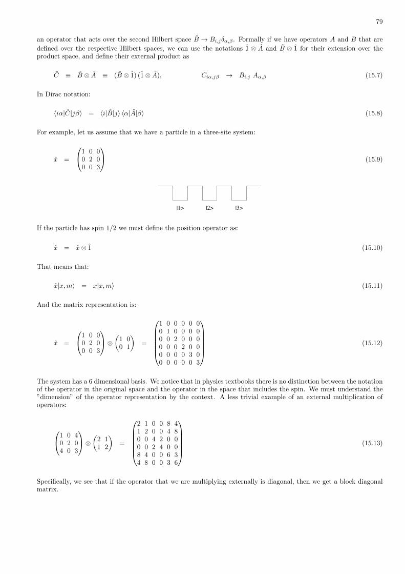
79

an operator that acts over the second Hilbert space B → Bi,jδα,β . Formally if we have operators A and B that are

defined over the respective Hilbert spaces, we can use the notations 1 ⊗ A and B ⊗ 1 for their extension over theproduct space, and define their external product as

C ≡ B ⊗ A ≡ (B ⊗ 1) (1⊗ A), Ciα,jβ → Bi,j Aα,β (15.7)

In Dirac notation:

〈iα|C|jβ〉 = 〈i|B|j〉 〈α|A|β〉 (15.8)

For example, let us assume that we have a particle in a three-site system:

x =

1 0 00 2 00 0 3

(15.9)

|1> |2> |3>

If the particle has spin 1/2 we must define the position operator as:

x = x⊗ 1 (15.10)

That means that:

x|x,m〉 = x|x,m〉 (15.11)

And the matrix representation is:

x =

1 0 00 2 00 0 3

⊗ (1 00 1

)=

1 0 0 0 0 00 1 0 0 0 00 0 2 0 0 00 0 0 2 0 00 0 0 0 3 00 0 0 0 0 3

(15.12)

The system has a 6 dimensional basis. We notice that in physics textbooks there is no distinction between the notationof the operator in the original space and the operator in the space that includes the spin. We must understand the”dimension” of the operator representation by the context. A less trivial example of an external multiplication ofoperators:

1 0 40 2 04 0 3

⊗ (2 11 2

)=

2 1 0 0 8 41 2 0 0 4 80 0 4 2 0 00 0 2 4 0 08 4 0 0 6 34 8 0 0 3 6

(15.13)

Specifically, we see that if the operator that we are multiplying externally is diagonal, then we get a block diagonalmatrix.

80

====== [15.3] External multiplication of spin spaces

Let us consider two operators in different Hilbert spaces L and S. The bases of the spaces are |m`〉, |ms〉. Theeigenvalues are m` = 0,±1 and ms = ±1/2. We label the new states as follows: | ⇑↑〉, | ⇑↓〉, | m↑〉, | m↓〉, | ⇓↑〉,| ⇓↓〉 This basis consists of 6 states. Therefore, each operator is represented by a 6× 6 matrix. For example:

Jx = Sx + Lx (15.14)

A mathematician would write it as follows:

Jx = 1⊗ Sx + Lx ⊗ 1 (15.15)

Let us consider for example the case ` = 1 and s = 1/2. In the natural basis we have

Sz →

11

1

⊗ 12

(1 00 −1

)=

1

2

1 00 −1

1 00 −1

1 00 −1

(15.16)

Sx →

11

1

⊗ 12

(0 11 0

)=

1

2

0 11 0

0 11 0

0 11 0

(15.17)

Lz →

1 0 00 0 00 0 −1

⊗ (11

)=

1 0 0

1 0 00 0 0

0 0 00 0 −1

0 0 −1

(15.18)

Lx →

0 1 01 0 10 1 0

⊗ (11

)=

0 1 0

0 1 01 0 1

1 0 10 1 0

0 1 0

(15.19)

etc. Empty entries means a zero value that is implied by the fact that the operator act only on the ”other” degree offreedom. This way of writing highlights the block structure of the matrices.

====== [15.4] Rotations of a Composite system

We assume that we have a spin ` entity whose states are represented by the basis

|m` = −`...+ `〉 (15.20)

and a spin s entity whose states are represented by the basis

|ms = −s...+ s〉 (15.21)

The natural (2`+ 1)× (2s+ 1) basis for the representation of the composite system is defined as

|m`,ms〉 = |m`〉 ⊗ |ms〉 (15.22)

81

A rotation of the ` entity is represented by the matrix

R = R` ⊗ 1 = e−iΦLn ⊗ 1 = e−iΦLn⊗1 (15.23)

We have used the identity f(A)⊗ 1 = f(A⊗ 1) which is easily established by considering the operation of both sideson a basis |a, b〉 that diagonalizes A. More generally we would like to rotate both the ` entity and the s entity. Thistwo operations commute since they act on different degrees of freedom (unlike two successive rotation of the sameentity). Thus we get

R = e−iΦ1⊗Sn e−iΦLn⊗1 = e−i~Φ·J (15.24)

where

J = L⊗ 1 + 1⊗ S = L+ S (15.25)

From now on we use the conventional sloppy notations of physicists as in the last equality: the space over which theoperator operates and the associated dimension of its matrix representation are implied by the context. Note that infull index notations the above can be summarized as follows:

〈m`ms|R|m′`m′s〉 = R`m`,m′`Rsms,m′s (15.26)

〈m`ms|Ji|m′`m′s〉 = [Li]m`,m′`δms,m′s + δm`,m′` [Si]ms,m′s (15.27)

====== [15.5] Addition of angular momentum

It is important to realize that the basis states |m`,ms〉 are eigenstates of Jz, but not of J2.

Jz∣∣m`,ms

⟩= (m` +ms)

∣∣m`,ms

⟩≡ mj

∣∣m`,ms

⟩(15.28)

J2∣∣m`,ms

⟩= superposition

[∣∣m`[±1],ms[∓1]⟩]

(15.29)

The second expression is based on the observation that

J2 = J2z +

1

2(J+J− + J−J+) (15.30)

J± = L± + S± (15.31)

This means that the representation is reducible, and can be written as a sum of irreducible representations. Using aconventional procedure we shall show later in this lecture that

(2`+ 1)⊗ (2s+ 1) = (2|`+ s|+ 1)⊕ · · · ⊕ (2|l − s|+ 1) (15.32)

It is called the ”addition of angular momentum” theorem. The output of the ”addition of angular momentum”procedure is a new basis |j,mj〉 that satisfies

J2|j,mj〉 = j(j + 1)|j,mj〉 (15.33)

Jz|j,mj〉 = mj |j,mj〉 (15.34)

In the next sections we learn how to make the following decompositions:

2⊗ 2 = 3⊕ 1 (15.35)

2⊗ 3 = 4⊕ 2

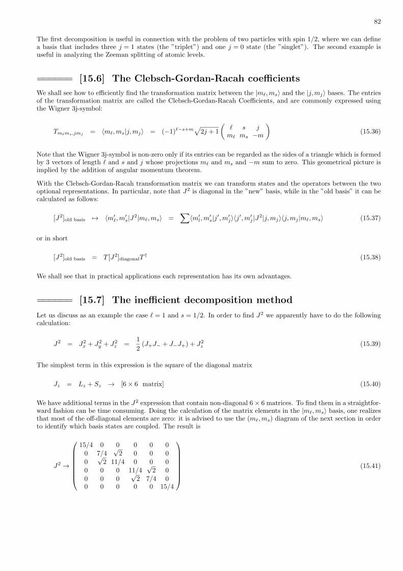
82

The first decomposition is useful in connection with the problem of two particles with spin 1/2, where we can definea basis that includes three j = 1 states (the ”triplet”) and one j = 0 state (the ”singlet”). The second example isuseful in analyzing the Zeeman splitting of atomic levels.

====== [15.6] The Clebsch-Gordan-Racah coefficients

We shall see how to efficiently find the transformation matrix between the |m`,ms〉 and the |j,mj〉 bases. The entriesof the transformation matrix are called the Clebsch-Gordan-Racah Coefficients, and are commonly expressed usingthe Wigner 3j-symbol:

Tm`ms,jmj = 〈m`,ms|j,mj〉 = (−1)`−s+m√

2j + 1

(` s jm` ms −m

)(15.36)

Note that the Wigner 3j-symbol is non-zero only if its entries can be regarded as the sides of a triangle which is formedby 3 vectors of length ` and s and j whose projections m` and ms and −m sum to zero. This geometrical picture isimplied by the addition of angular momentum theorem.

With the Clebsch-Gordan-Racah transformation matrix we can transform states and the operators between the twooptional representations. In particular, note that J2 is diagonal in the ”new” basis, while in the ”old basis” it can becalculated as follows:

[J2]old basis 7→ 〈m′`,m′s|J2|m`,ms〉 =∑〈m′l,m′s|j′,m′j〉〈j′,m′j |J2|j,mj〉〈j,mj |m`,ms〉 (15.37)

or in short

[J2]old basis = T [J2]diagonalT† (15.38)

We shall see that in practical applications each representation has its own advantages.

====== [15.7] The inefficient decomposition method

Let us discuss as an example the case ` = 1 and s = 1/2. In order to find J2 we apparently have to do the followingcalculation:

J2 = J2x + J2

y + J2z =

1

2(J+J− + J−J+) + J2

z (15.39)

The simplest term in this expression is the square of the diagonal matrix

Jz = Lz + Sz → [6× 6 matrix] (15.40)

We have additional terms in the J2 expression that contain non-diagonal 6× 6 matrices. To find them in a straightfor-ward fashion can be time consuming. Doing the calculation of the matrix elements in the |m`,ms〉 basis, one realizesthat most of the off-diagonal elements are zero: it is advised to use the (m`,ms) diagram of the next section in orderto identify which basis states are coupled. The result is

J2 →

15/4 0 0 0 0 0

0 7/4√

2 0 0 0

0√

2 11/4 0 0 0

0 0 0 11/4√

2 0

0 0 0√

2 7/4 00 0 0 0 0 15/4

(15.41)

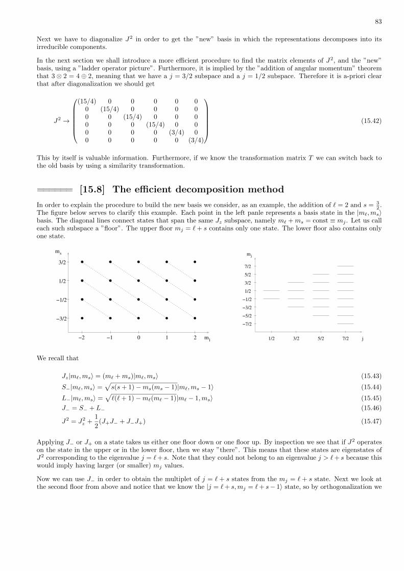
83

Next we have to diagonalize J2 in order to get the ”new” basis in which the representations decomposes into itsirreducible components.

In the next section we shall introduce a more efficient procedure to find the matrix elements of J2, and the ”new”basis, using a ”ladder operator picture”. Furthermore, it is implied by the ”addition of angular momentum” theoremthat 3 ⊗ 2 = 4 ⊕ 2, meaning that we have a j = 3/2 subspace and a j = 1/2 subspace. Therefore it is a-priori clearthat after diagonalization we should get

J2 →

(15/4) 0 0 0 0 0

0 (15/4) 0 0 0 00 0 (15/4) 0 0 00 0 0 (15/4) 0 00 0 0 0 (3/4) 00 0 0 0 0 (3/4)

(15.42)

This by itself is valuable information. Furthermore, if we know the transformation matrix T we can switch back tothe old basis by using a similarity transformation.

====== [15.8] The efficient decomposition method

In order to explain the procedure to build the new basis we consider, as an example, the addition of ` = 2 and s = 32 .

The figure below serves to clarify this example. Each point in the left panle represents a basis state in the |m`,ms〉basis. The diagonal lines connect states that span the same Jz subspace, namely m` +ms = const ≡ mj . Let us calleach such subspace a ”floor”. The upper floor mj = `+ s contains only one state. The lower floor also contains onlyone state.

ms

lm

3/2

1/2

−1/2

−3/2

210−1−2

jm

1/2 3/2 5/2 7/2

−1/2

7/25/23/21/2

−3/2

−7/2−5/2

j

We recall that

Jz|m`,ms〉 = (m` +ms)|m`,ms〉 (15.43)

S−|m`,ms〉 =√s(s+ 1)−ms(ms − 1)|m`,ms − 1〉 (15.44)

L−|m`,ms〉 =√`(`+ 1)−m`(m` − 1)|m` − 1,ms〉 (15.45)

J− = S− + L− (15.46)

J2 = J2z +

1

2(J+J− + J−J+) (15.47)

Applying J− or J+ on a state takes us either one floor down or one floor up. By inspection we see that if J2 operateson the state in the upper or in the lower floor, then we stay ”there”. This means that these states are eigenstates ofJ2 corresponding to the eigenvalue j = `+ s. Note that they could not belong to an eigenvalue j > `+ s because thiswould imply having larger (or smaller) mj values.

Now we can use J− in order to obtain the multiplet of j = ` + s states from the mj = ` + s state. Next we look atthe second floor from above and notice that we know the |j = `+ s,mj = `+ s− 1〉 state, so by orthogonalization we

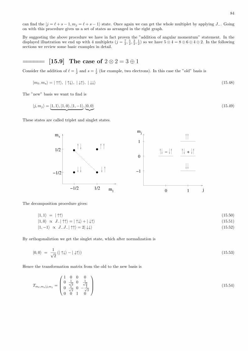
84

can find the |j = `+ s− 1,mj = `+ s− 1〉 state. Once again we can get the whole multiplet by applying J−. Goingon with this procedure gives us a set of states as arranged in the right graph.

By suggesting the above procedure we have in fact proven the ”addition of angular momentum” statement. In thedisplayed illustration we end up with 4 multiplets (j = 7

2 ,52 ,

32 ,

12 ) so we have 5⊗ 4 = 8⊕ 6⊕ 4⊕ 2. In the following

sections we review some basic examples in detail.

====== [15.9] The case of 2⊗ 2 = 3⊕ 1

Consider the addition of ` = 12 and s = 1

2 (for example, two electrons). In this case the ”old” basis is

|m`,ms〉 = | ↑↑〉, | ↑↓〉, | ↓↑〉, | ↓↓〉 (15.48)

The ”new” basis we want to find is

|j,mj〉 = |1, 1〉, |1, 0〉, |1,−1〉︸ ︷︷ ︸, |0, 0〉︸ ︷︷ ︸ (15.49)

These states are called triplet and singlet states.

ms

lm

−1/2

1/2

1/2−1/2

jm

0

1

−1

10 j

− +

The decomposition procedure gives:

|1, 1〉 = | ↑↑〉 (15.50)

|1, 0〉 ∝ J−| ↑↑〉 = | ↑↓〉+ | ↓↑〉 (15.51)

|1,−1〉 ∝ J−J−| ↑↑〉 = 2| ↓↓〉 (15.52)

By orthogonaliztion we get the singlet state, which after normalization is

|0, 0〉 =1√2

(| ↑↓〉 − | ↓↑〉) (15.53)

Hence the transformation matrix from the old to the new basis is

Tm`,ms|j,mj =

1 0 0 00 1√

20 1√

2

0 1√2

0 − 1√2

0 0 1 0

(15.54)

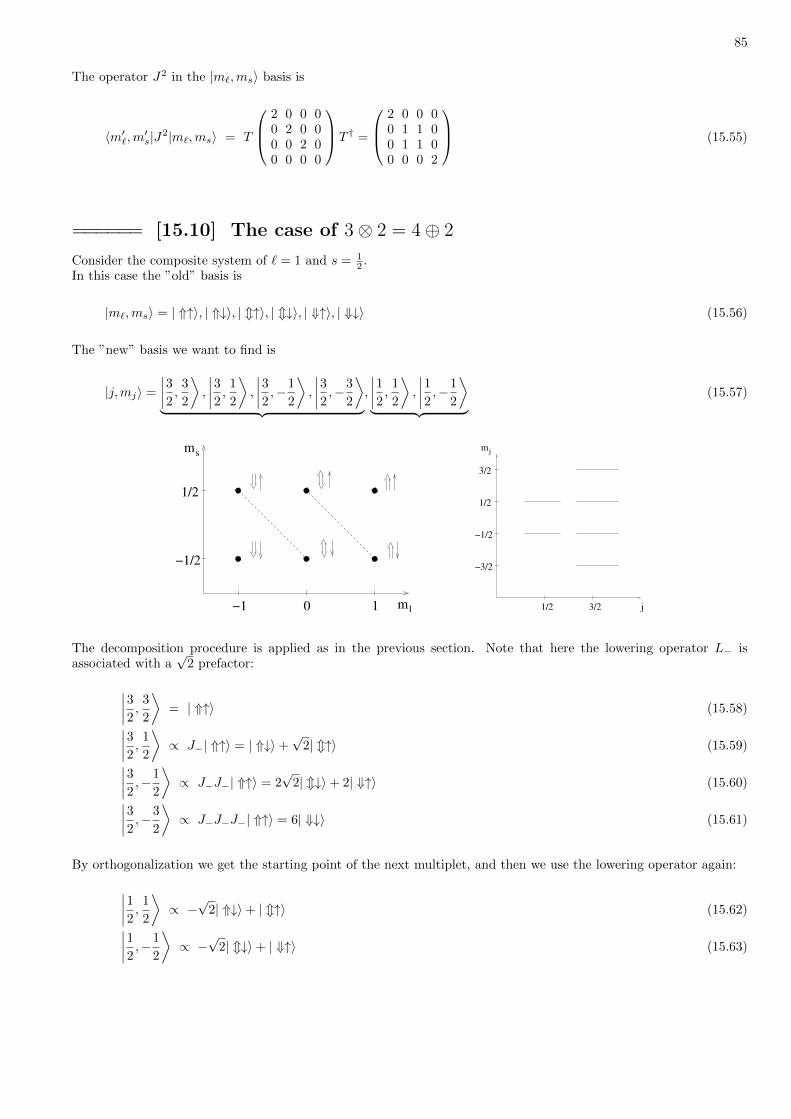
85

The operator J2 in the |m`,ms〉 basis is

〈m′`,m′s|J2|m`,ms〉 = T

2 0 0 00 2 0 00 0 2 00 0 0 0

T † =

2 0 0 00 1 1 00 1 1 00 0 0 2

(15.55)

====== [15.10] The case of 3⊗ 2 = 4⊕ 2

Consider the composite system of ` = 1 and s = 12 .

In this case the ”old” basis is

|m`,ms〉 = | ⇑↑〉, | ⇑↓〉, | m↑〉, | m↓〉, | ⇓↑〉, | ⇓↓〉 (15.56)

The ”new” basis we want to find is

|j,mj〉 =

∣∣∣∣32 , 3

2

⟩,

∣∣∣∣32 , 1

2

⟩,

∣∣∣∣32 ,−1

2

⟩,

∣∣∣∣32 ,−3

2

⟩︸ ︷︷ ︸,

∣∣∣∣12 , 1

2

⟩,

∣∣∣∣12 ,−1

2

⟩︸ ︷︷ ︸ (15.57)

lm

sm

10−1

−1/2

1/2

jm

1/2

−1/2

−3/2

1/2

3/2

j3/2

The decomposition procedure is applied as in the previous section. Note that here the lowering operator L− isassociated with a

√2 prefactor:

∣∣∣∣32 , 3

2

⟩= | ⇑↑〉 (15.58)∣∣∣∣32 , 1

2

⟩∝ J−| ⇑↑〉 = | ⇑↓〉+

√2| m↑〉 (15.59)∣∣∣∣32 ,−1

2

⟩∝ J−J−| ⇑↑〉 = 2

√2| m↓〉+ 2| ⇓↑〉 (15.60)∣∣∣∣32 ,−3

2

⟩∝ J−J−J−| ⇑↑〉 = 6| ⇓↓〉 (15.61)

By orthogonalization we get the starting point of the next multiplet, and then we use the lowering operator again:

∣∣∣∣12 , 1

2

⟩∝ −

√2| ⇑↓〉+ | m↑〉 (15.62)∣∣∣∣12 ,−1

2

⟩∝ −

√2| m↓〉+ | ⇓↑〉 (15.63)

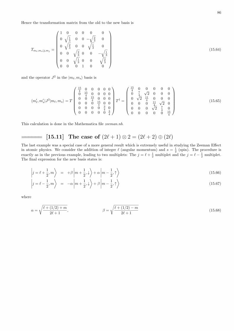
86

Hence the transformation matrix from the old to the new basis is

Tm`,ms|j,mj =

1 0 0 0 0 0

0√

13 0 0 −

√23 0

0√

23 0 0

√13 0

0 0√

23 0 0 −

√13

0 0√

13 0 0

√23

0 0 0 1 0 0

(15.64)

and the operator J2 in the |m`,ms〉 basis is

〈m′`,m′s|J2|m`,ms〉 = T

154 0 0 0 0 00 15

4 0 0 0 00 0 15

4 0 0 00 0 0 15

4 0 00 0 0 0 3

4 00 0 0 0 0 3

4

T † =

154 0 0 0 0 0

0 74

√2 0 0 0

0√

2 114 0 0 0

0 0 0 114

√2 0

0 0 0√

2 74 0

0 0 0 0 0 154

(15.65)

This calculation is done in the Mathematica file zeeman.nb.

====== [15.11] The case of (2`+ 1)⊗ 2 = (2`+ 2)⊕ (2`)

The last example was a special case of a more general result which is extremely useful in studying the Zeeman Effectin atomic physics. We consider the addition of integer ` (angular momentum) and s = 1

2 (spin). The procedure is

exactly as in the previous example, leading to two multiplets: The j = ` + 12 multiplet and the j = ` − 1

2 multiplet.The final expression for the new basis states is:

∣∣∣∣j = `+1

2,m

⟩= +β

∣∣∣∣m+1

2, ↓⟩

+ α

∣∣∣∣m− 1

2, ↑⟩

(15.66)∣∣∣∣j = `− 1

2,m

⟩= −α

∣∣∣∣m+1

2, ↓⟩

+ β

∣∣∣∣m− 1

2, ↑⟩

(15.67)

where

α =

√`+ (1/2) +m

2`+ 1, β =

√`+ (1/2)−m

2`+ 1(15.68)

87

[16] Galilei group and the non-relativistic Hamiltonian

====== [16.1] The Representation of the Galilei Group

The defining realization of the Galilei group is over phase space. Accordingly, that natural representation is withfunctions that ”live” in phase space. Thus the a-translated ρ(x, v) is ρ(x−a, v) while the u-boosted ρ(x, v) is ρ(x, v−u)etc.

The generators of the displacements are denoted Px,Py,Pz, the generators of the boosts are denoted Qx,Qy,Qz,and the generators of the rotations are denoted Jx,Jy,Jz. Thus we have 9 generators. It is clear that translationsand boosts commute, so the only non-trivial structure constants of the Lie algebra have to do with the rotations:

[Pi,Pj ] = 0 (16.1)

[Qi,Qj ] = 0 (16.2)

[Pi,Qj ] = 0 (to be discussed) (16.3)

[Ji,Aj ] = iεijkAk for A = P,Q, J (16.4)

Now we ask the following question: is it possible to find a faithful representation of the Galilei group that ”lives”in configuration space. We already know that the answer is ”almost” positive: We can represent pure quantumstates using ”wavefunctions” ψ(x). These wavefunctions can be translated and rotated. On a physical basis itis also clear that we can talk about ”boosted” states: this means to give the particle a different velocity. So wecan also boost wavefunctions. On physical grounds it is clear that the boost should not change |ψ(x)|2. In factit is not difficult to figure out that the boost is realized by a multiplication of ψ(x) by ei(mu)x. Hence we get theidentifications Px 7→ −i(d/dx) and Qx 7→ −mx for the generators. Still the wise reader should realize that in this”new” representation boosts and translations do not commute, while in case of the strict phase space realization theydo commute!

On the mathematical side it would be nice to convince ourselves that the price of not having commutation betweentranslations and boosts is inevitable, and that there is a unique representation (up to a gauge) of the Galilei group using”wavefunctions”. This mathematical discussion should clarify that the ”compromise” for having such a representationis: (1) The wavefunctions have to be complex; (2) The boosts commute with the translations only up to a phase factor.

We shall see that the price that we have to pay is to add 1 as a tenth generator to the Lie algebra. This is similarto the discussion of the relation between SO(3) and SU(2). The elements of the latter can be regarded as ”rotations”provided we ignore an extra ”sign factor”. Here rather than ignoring a ”sign factor” we have to ignore a complex”phase factor”.

Finally, we shall see that the most general form of the non-relativistic Hamiltonian of a spinless particle, and inparticular its mass, are implied by the structure of the quantum Lie algebra.

====== [16.2] The Mathematical Concept of Mass

An element τ of the Galilei group is parametrized by 9 parameters. To find a strict (unitary) representation meansto associate with each element a linear operator U(τ) such that τ1 ⊗ τ2 = τ3 implies

U(τ1)U(τ2) = U(τ3) (16.5)

Let us see why this strict requirement cannot be realized if we want a representation with ”wavefunctions”. Supposethat we have an eigenstate of P such that P |k〉 = k|k〉. since we would like to assume that boosts commute with

translations it follows that also Uboost|k〉 is an eigenstate of P with the same eigenvalue. This is absurd, becauseit is like saying that a particle has the same momentum in all reference frames. So we have to replace the strictrequirement by

U(τ1)U(τ2) = ei×phaseU(τ3) (16.6)

88

This means that now we have an extended group that ”covers” the Galilei group, where we have an additionalparameter (a phase), and correspondingly an additional generator (1). The Lie algebra of the ten generators ischaracterized by

[Gµ, Gν ] = i∑λ

cλµνGλ (16.7)

where G0 = 1 and the other nine generators are Pi, Qi, Ji with i = x, y, z. It is not difficult to convince ourselvesthat without loss of generality this introduces one ”free” parameter into the algebra (the other additional structureconstants can be set to zero via appropriate re-definition of the generators). The ”free” non-trivial structure constantm appears in the commutation

[Pi,Qj ] = imδij (16.8)

which implies that boosts do not commute with translations.

====== [16.3] Finding the Most General Hamiltonian

Assume that we have a spinless particle for which the standard basis for representation is |x〉. With appropriate gaugeof the x basis the generator of the translations is P 7→ −i(d/dx). From the commutation relation [P,Q] = im wededuce that Q = −mx+ g(p), where g() is an arbitrary function. With appropraite gauge of the momentum basis wecan assume Q = −mx.

The next step is to observe that the effect of a boost on the velocity operator should be

Uboost(u)−1vUboost(u) = v + u (16.9)

which implies that [Q, v] = −i. The simplest possibility is v = p/m. But the most general possibility is

v =1

m(p−A(x)) (16.10)

where A is an arbitrary function. This time we cannot gauge away A.

The final step is to recall the rate of change formula which implies the relation v = i[H, x]. The simplest operatorthat will give the desired result for v is H = 1

2m (p − A(x))2. But the most general possibility involves a secondundetermined function:

H =1

2m(p−A(x))2 + V (x) (16.11)

Thus we have determined the most general Hamiltonian that agrees with the Lie algebra of the Galilei group. In thenext sections we shall see that this Hamiltonian is indeed invariant under Galilei transformations.

89

[17] Transformations and invariance

====== [17.1] Transformation of the Hamiltonian

First we would like to make an important distinction between passive [”Heisenberg”] and active [”Schrodinger”] pointsof view regarding transformations. The failure to appreciate this distinction is an endless source of confusion.

In classical mechanics we are used to the passive point of view. Namely, to go to another reference frame (say adisplaced frame) is like a change of basis. Namely, we relate the new coordinates to the old ones (say x = x− a), andin complete analogy we relate the new basis |x〉 to the old basis |x〉 by a transformation matrix T = e−iap such that|x〉 = T |x〉 = |x+ a〉.

However we can also use an active point of view. Rather than saying that we ”change the basis” we can say that we”transform the wavefunction”. It is like saying that ”the tree is moving backwards” instead of saying that ”the car ismoving forward”. In this active approach the transformation of the wavefunction is induced by S = T−1, while theobservables stay the same. So it is meaningless to make a distinction between old (x) and new (x) coordinates!

From now on we use the more convenient active point of view. It is more convenient because it is in the spirit of theSchrodinger (rather than Heisenberg) picture. In this active point of view observables do not transform. Only thewavefunction transforms (”backwards”). Below we discuss the associated transformation of the evolution operatorand the Hamiltonian.

Assume that the transformation of the state as we go from the ”old frame” to the ”new frame” is ψ = Sψ. Theevolution operator that propagates the state of the system from t0 to t in the new frame is:

U(t, t0) = S(t)U(t, t0)S−1(t0) (17.1)

The idea is that we have to transform the state to the old frame (laboratory) by S−1, then calculate the evolutionthere, and finally go back to our new frame. We recall that the Hamiltonian is defined as the generator of theevolution. By definition

U(t+ δt, t0) = (1− iδtH(t))U(t, t0) (17.2)

Hence

H = i∂U

∂tU−1 = i

[∂S (t)

∂tUS (t0)

−1+ S(t)

∂U

∂tS(t0)−1

]S(t0)U−1S(t)−1 (17.3)

and we get the result

H = SHS−1 + i∂S

∂tS−1 (17.4)

In practice we assume a Hamiltonian of the form H = h(x, p;V,A). Hence we get that the Hamiltonian in the newframe is

H = h(SxS−1, SpS−1;V,A) + i∂S

∂tS−1 (17.5)

Recall that ”invariance” means that the Hamiltonian keeps its form, but the fields in the Hamiltonian may havechanged. So the question is whether we can write the new Hamiltonian as

H = h(x, p; A, V ) (17.6)

90

To have ”symmetry” rather than merely ”invariance” means that the Hamiltonian remains the same with A = A andV = V . We are going to show that the following Hamiltonian is invariant under translations, rotations, boosts andgauge transformations:

H =1

2m

(p− ~A(x)

)2

+ V (x) (17.7)

We shall argue that this is the most general non-relativistic Hamiltonian for a spinless particle. We shall also discussthe issue of time reversal (anti-unitary) transformations.

====== [17.2] Invariance Under Translations

T = D(a) = e−iap (17.8)

S = T−1 = eiap

The coordinates (basis) transform with T , while the wavefunctions are transformed with S.

SxS−1 = ˆx+ a (17.9)

SpS−1 = p

Sf(x, p)S−1 = f(SxS−1, SpS−1) = f(x+ a, p)

(17.10)

Therefore the Hamiltonian is invariant with

V (x) = V (x+ a) (17.11)

A(x) = A(x+ a)

====== [17.3] Invariance Under Gauge

T = e−iΛ(x) (17.12)

S = eiΛ(x)

SxS−1 = x

SpS−1 = p−∇Λ(x)

Sf(x, p)S−1 = f(SxS−1, SpS−1) = f(x, p−∇Λ(x))

Therefore the Hamiltonian is invariant with

V (x) = V (x) (17.13)

A(x) = A(x) +∇Λ(x)

Note that the electric and the magnetic fields are not affected by this transformation.

91

More generally we can consider time dependent gauge transformations with Λ(x, t). Then we get in the ”new”Hamiltonian an additional term, leading to

V (x) = V (x)− (d/dt)Λ(x, t) (17.14)

A(x) = A(x) +∇Λ(x, t)

In particular we can use the very simple gauge Λ = ct in order to change the Hamiltonian by a constant (H = H− c).

====== [17.4] Boosts and Transformations to a Moving System

From an algebraic point of view a boost can be regarded as a special case of gauge:

T = ei(mu)x (17.15)

S = e−i(mu)x

SxS−1 = x

SpS−1 = p+ mu

Hence V (x) = V (x) and A(x) = A(x)−mu. But a transformation to a moving frame is not quite the same thing. Thelatter combines a boost and a time dependent displacement. The order of these operations is not important becausewe get the same result up to a constant phase factor that can be gauged away:

S = eiphase(u) e−i(mu)x ei(ut)p (17.16)

SxS−1 = x+ ut

SpS−1 = p+ mu

The new Hamiltonian is

H = SHS−1 + i∂S

∂tS−1 = SHS−1 − up =

1

2m(p− A(x))2 + V (x) + const(u) (17.17)

where

V (x, t) = V (x+ ut, t)− u ·A(x+ ut, t) (17.18)

A(x, t) = A(x+ ut, t)

Thus in the new frame the magnetic field is the same (up to the displacement) while the electric field is:

E = −∂A∂t−∇V = E + u× B (17.19)

In the derivation of the latter we used the identity

∇(u ·A)− (u · ∇)A = u× (∇×A) (17.20)

Finally we note that if we do not include the boost in S, then we get essentially the same results up to a gauge. Byincluding the boost we keep the same dispersion relation: If in the lab frame A = 0 and we have v = p/m, then in

the new frame we also have A = 0 and therefore v = p/m still holds.

====== [17.5] Transformations to a rotating frame

Let us assume that we have a spinless particle held by a a potential V (x). Assume that we transform to a rotatingframe. We shall see that the transformed Hamiltonian will have in it a Coriolis force and a centrifugal force.

92

The transformation that we consider is

S = ei(~Ωt)·L (17.21)

The new Hamiltonian is

H = SHS−1 + i∂S

∂tS−1 =

1

2mp2 + V (x)− Ω · L (17.22)

It is implicit that the new x coordinate is relative to the rotating frame of reference. Without loss of generality we

assume ~Ω = (0, 0,Ω). Thus we got Hamiltonian that looks very similar to that of a particle in a uniform magneticfield (see appropriate lecture):

H =1

2m(p−A(x))2 + V (x) =

p2

2m− B

2mLz +

B2

8m(x2 + y2) + V (x) (17.23)

The Coriolis force is the ”magnetic field” B = 2mΩ. By adding and subtracting a quadratic term we can write theHamiltonian H in the standard way with

V = V − 1

2mΩ2(x2 + y2) (17.24)

A = A+ m~Ω× r

The extra −(1/2)mΩ2(x2 + y2) term is called the centrifugal potential.

====== [17.6] Time Reversal transformations

Assume for simplicity that the Hamiltonian is time independent. The evolution operator is U = e−iHt. If we make aunitary transformation T we get

U = T−1e−iHtT = e−i(T−1HT )t = e−iHt (17.25)

where H = T−1HT . Suppose we want to reverse the evolution in our laboratory. Apparently we have to engineerT such that T−1HT = −H. If this can be done the propagator U will take the system backwards in time. We canname such T operation a ”Maxwell demon” for historical reasons. Indeed for systems with spins such transformationshave been realized using NMR techniques. But for the ”standard” Hamiltonian H = p2/(2m) it is impossible to finda unitary transformation that do the trick for a reason that we explain below.

At first sight it seems that in classical mechanics there is a transformation that reverses the dynamics. All we haveto do is to invert the sign of the velocity. Namely p 7→ −p while x 7→ x. So why not to realize this transformationin the laboratory? This was Loschmidt’s claim against Boltzman. Boltzman’s answer was ”go and do it”. Why is it”difficult” to do? Most people will probably say that to reverse the sign of an Avogadro number of particles is tough.But in fact there is a better answer. In a sense it is impossible to reverse the sign even of one particle! If we believethat the dynamics of the system are realized by a Hamiltonian, then the only physical transformations are propercanonical transformations. Such transformations preserves the Poisson brackets, whereas p 7→ −p, x 7→ x invertssign. So it cannot be physically realized.

In quantum mechanical language we say that any physical realizable evolution process is described by a unitaryoperator. We claim that the transformation p 7→ −p while x 7→ x cannot be realized by any physical Hamiltonian.Assume that we have a unitary transformation T such that T pT−1 = −p while T xT−1 = x. This would implyT [x, p]T−1 = −[x, p]. So we get i = −i. This means that such a transformation does not exist.

But there is a way out. Wigner has proved that there are two types of transformations that map states in Hilbertspace such that the overlap between states remains the same. These are either unitary transformations or anti-unitary

93

transformations. The time reversal transformations that we are going to discuss are anti-unitary. They cannot berealized in an actual laboratory experiment. This leads to the distinction between ”microreversibility” and actual”reversibility”: It is one thing to say that a Hamiltonian has time reversal symmetry. It is a different story to actuallyreverse the evolution.

We shall explain in the next section that the ”velocity reversal” transformation that has been mentioned above canbe realized by an antiunitary transformation. We also explain that in the case of an antiunitary transformation weget

U = T−1e−iHtT = e+i(T−1HT )t = e−iHt (17.26)

where H = −T−1HT . Thus in order to reverse the evolution we have to engineer T such that T−1HT = H, orequivalently [H, T ] = 0. If such a T exists then we say that H has time reversal symmetry. In particular we shallexplain that in the absence of a magnetic field the non-relativistic Hamiltonian has a time reversal symmetry.

There is a subtle distinction between the physical notion of time reversal invariance, as opposed to invariance underunitary operation. In the latter case, say ”rotation”, the given transformation T is well defined irrespective of thedynamics. Then we can check whether the ”physical law” of the dynamics is ”invariant”

Given T , ∀A, ∃A, T−1U [A]T = U [A] (17.27)

In contrast to that time reversal invariance means:

∃T, ∀A, ∃A, U [A]−1 = TU [A]T−1 (17.28)

For example, if A is the vector potential, time reversal invariance implies the transformation A = −A, which meansthat the time reversed dynamics can be realized by inverting the magnetic field. Thus, the definition of time reversaltransformation is implied by the dynamics, and cannot be introduced out of context.

====== [17.7] Anti-unitary Operators

An anti-unitary operator has an anti-linear rather than linear property. Namely,

T (α |φ〉+ β |ψ〉) = α∗T |φ〉+ β∗T |ψ〉 (17.29)

An anti-unitary operator can be represented by a matrix Tij whose columns are the images of the basis vectors.Accordingly |ϕ〉 = T |ψ〉 implies ϕi = Tijψ

∗j . So its operation is complex conjugation followed by linear transformation.

It is useful to note that H = T−1HT implies Hµν = T ∗iµH∗ijTjν . This is proved by pointing out that the effect of double

complex conjugation when operating on a vector is canceled as far as its elements are concerned.

The simplest procedure to construct an anti-unitary operator is as follows: We pick an arbitrary basis |r〉 and definea diagonal anti-unitary operator K that is represented by the unity matrix. Such operator maps ψr to ψ∗r , and has

the property K2 = 1. Note also that for such operator Hij = H∗ij . In a sense there is only one anti-unitary operator

per choice of a basis. Namely, assume that T is represented by the diagonal matrix eiφr. That means

T |r〉 = eiφr |r〉 (17.30)

Without loss of generality we can assume that φr = 0. This is because we can gauge the basis. Namely, we can definea new basis |r〉 = eiλr |r〉 for which

T |r〉 = ei(φr−2λr) |r〉 (17.31)

By setting λr = φr/2 we can make all the eigenvalues equal to one, and hence T = K. Any other antiunitaryoperator can be written trivially as T = (TK)K where TK is unitary. So in practice any T is represented by complex

94

conjugation followed by a unitary transformation. Disregarding the option of having the ”extra” unitary operation,time reversal symmetry T−1HT = H means that in the particular basis where T is diagonal the Hamiltonian matrixis real (H∗r,s = Hr,s), rather than complex.

Coming back to the ”velocity reversal” transformation it is clear that T should be diagonal in the position basis (xshould remain the same). Indeed we can verify that such a T automatically reverses the sign of the momentum:

|k〉 =∑x

eikx |x〉 (17.32)

T |k〉 =∑x

T eikx |x〉 =∑x

e−ikx |x〉 = |−k〉

In the absence of a magnetic field the kinetic term p2 in the Hamiltonian has symmetry with respect to this T .Therefore we say that in the absence of a magnetic field we have time reversal symmetry. In which case the Hamiltonianis real in the position representation.

What happens if we have a magnetic field? Does it mean that there is no time reversal symmetry? Obviously inparticular cases the Hamiltonian may have a different anti-unitary symmetry: if V (−x) = V (x) then the Hamiltonianis symmetric with respect to the transformation x 7→ −x while p 7→ p. The anti-unitary T in this case is diagonal inthe p representation. It can be regarded as a product of ”velocity reversal” and ”inversion” (x 7→ −x and p 7→ −p).The former is anti-unitary while the latter is a unitary operation.

If the particle has a spin we can define K with respect to the standard basis. The standard basis is determined byx and σ3. However, T = K is not the standard time reversal symmetry: It reverse the polarization if it is in theY direction, but leave it unchanged if it is in the Z or in the X direction. We would like to have T−1σT = −σ. Thisimplies that

T = e−iπSyK = −iσyK (17.33)

Note that T 2 = (−1)N where N is the number of spin 1/2 particles in the system. This implies Kramers degeneracyfor odd N . The argument goes as follows: If ψ is an eigenstate of the Hamiltonian, then symmetry with respect to Timplies that also Tψ is an eigenstate. Thus we must have a degeneracy unless Tψ = λψ, where λ is a phase factor.But this would imply that T 2ψ = λ2ψ while for odd N we have T 2 = −1. The issue of time reversal for particles withspin is further discussed in [Messiah p.669].

95

Dynamics and Driven Systems

[18] Transition probabilities

====== [18.1] Time dependent Hamiltonians

To find the evolution which is generated by a time independent Hamiltonian is relatively easy. Such a Hamiltonianhas eigenstates |n〉 which are the ”stationary” states of the system. The evolution in time of an arbitrary state is:

|ψ(t)〉 =∑n

e−iEntψn|n〉 (18.1)

But in general the Hamiltonian can be time-dependent [H(t1),H(t2)] 6= 0. In such case the strategy that was describedabove for finding the evolution in time loses its significance. In this case, there is no simple expression for the evolutionoperator:

U(t, t0) = e−idtNH(tN ) · · · e−idt2H(t2)e−idt1H(t1) ≡ Texp

[−i∫ t

t0

H(t′)dt′]

(18.2)

where Texp denotes time-ordered exponential, that can be replaced by the ordinary exp if H is constant, but not ingeneral.

Of special interest is the case where the Hamiltonian can be written as the sum of a time independent part H0 and atime dependent perturbation V (t). In such case we can make the substitution

e−idtnH(tn) = e−idtnH0 (1− idtnV (tn)) (18.3)

Next we can expand and rearrange the Texp sum as follows:

U(t) = U0(t, t0) + (−i)∫t0<t1<t

dt1 U0(t, t1)V (t1)U0(t1, t0) (18.4)

+ (−i)2x

t0<t1<t2<t

dt2dt1 U0(t, t2)V (t2)U0(t2, t1)V (t1)U0(t1, t0) + · · · (18.5)

There are few cases where the calculation can be carried out analytically to infinite order (a nice example is theLandau-Zener problem). In many case, if the perturbation is weak enough, one is satisfied with the leading orderapproximation. Below we assume that the Hamiltonian can be written as a sum of a time independent part H0 anda time dependent perturbation. Namely,

H = H0 + V = H0 + f(t)W (18.6)

Using first order perturbation theory, we shall introduce a formula for calculating the probability of transition betweenunperturbed eigenstates. The formula can be obtained directly in ”one line” derivation from the above expansion.But for pedagogical reason we shall repeat its derivation using a traditional iterative scheme.

====== [18.2] The interaction picture

We would like to work in a basis such that H0 is diagonal:

H0|n〉 = En|n〉 (18.7)

|Ψ(t)〉 =∑n

Ψn(t) |n〉

96

The evolution is determined by the Schrodinger’s equation:

idψndt

= Enψn +∑n′

Vnn′Ψn′ (18.8)

which can be written in a matrix style as follows:

id

dt

Ψ1

Ψ2

...

=

E1Ψ1

E2Ψ2

...

+

V11 V12 · · ·V21 V22 · · ·

......

. . .

Ψ1

Ψ2

...

(18.9)

Without the perturbation we would get ψn(t) = cne−iEnt, where cn are constants. It is therefore natural to use thevariation of parameters method, and to write

Ψn(t) = cn(t) e−iEnt (18.10)

In other words, we represent the ”wave function” by the amplitudes cn(t) = ψn(t)eiEnt rather than by the amplitudesΨn(t). The Schrodinger’s equation in the new representation takes the form

idcndt

=∑n′

ei(En−En′ )t Vnn′ cn′(t) (18.11)

This is called the Schrodinger’s equation in the ”interaction picture”. It is a convenient equation because the termon the right is assumed to be ”small”. Therefore, the amplitudes cn(t) change slowly. This equation can be solvedusing an iterative scheme which leads naturally to a perturbative expansion. The iteration are done with the integralversion of the above equation:

cn(t) = cn(0) − i∑n′

∫ t

0

eiEnn′ t′Vn,n′ cn′(t

′) dt′ (18.12)

where Enn′ = En − En′ . In each iteration we get the next order. Let us assume that the system has been preparedin level n0. This means that the zero order solution is

c[0]n (t) = cn(0) = δn,n0 (18.13)

We iterate once and get the first-order solution:

cn(t) = δn,n0 − i∫ t

0

eiEnn0t′Vn,n0dt

′ (18.14)

It is instructive to consider constant perturbation (V does not depend on time). Doing the integral and going backto the standard representation we get the following result for the first-order transition amplitude:

ψn(t) = Vn,n0

e−iEnt − e−iEn0 t

En − En0

, [constant perturbation, n 6= n0] (18.15)

We notice that for very short times we get ψn(t) ≈ −iVn,n0t, which reflects the definition of the matrix elements of

the Hamiltonian as the ”hopping” amplitude per unit of time. As long as the energy difference (En − En0) is not

resolved, this expression is merely modulated ψn(t) ≈ [−iVn,n0t]e−iEnt, reflecting the choice of the energy reference.

97

But for longer times the accumulation of the amplitude is suppressed due to the temporal oscillations of the integrand.If the perturbation is constant, the oscillation frequency of the integrand is ω = (En − En′). If the perturbation ischaracterized by a frequency Ω, this oscillation frequency becomes ν = (En − En′ − Ω).

In order to illustrate the effect of the oscillating integrand, consider a problem in which the unperturbed Hamiltonianis ”to be in some site”. We can regard the possibility to move from site to site as a perturbation. The energydifferences in the site problem are the gradients of the potential energy, which we call “electric field”. The hoppingamplitude is the same in each ”hop” even if the hop into a potential wall. However, due to the potential differencethe probability amplitude does not ”accumulate” and therefore the particle is likely to be reflected. The reflection isnot due to the lack of coupling between site, but due to the potential difference that induces “fields” that suppressesthe transition probability.

====== [18.3] The transition probability formula

The expression we found for the wavefunction amplitudes using first-order perturbation theory can be written as:

cn(t) ≈ 1 for n = n0 (18.16)

cn(t) = −iWn,n0

∫ t

0

f(t′)eiEnn0 t′dt′ otherwise (18.17)

The latter expression for the transition amplitude can be written optionally as a Fourier transform (FT):

cn(t) ≈ −iWn,n0FT [f(t)] (18.18)

We use here the convention that f(t) = 0 before and after the pulse. For example, if we turn on a constant perturbationfor a finite duration, then f(t) is a rectangle function. It is implicit that the FT is calculated at the frequency of thetransition ω = En − En0

, namely,

FT [f(t)] =

∫ ∞−∞

f(t′) eiEn,n0 t′dt′ (18.19)

The associated expression for the transition probability is:

Pt(n|n0) ≈ |Wn,n0 |2 ×∣∣∣FT [f(t)]

∣∣∣2 (18.20)

====== [18.4] The effect of a constant or harmonic perturbation

We consider the following scenario: A particle is prepared in the state n0, and then a constant perturbation is turnedon for a time t. We want to know what is the probability of finding the particle at some later time in the state n.Using the transition probability formula we get

Pt(n|n0) = |cn(t)|2 = |Wnn0|2∣∣∣∣1− ei(En−En0

)t

En − En0

∣∣∣∣2 (18.21)

We notice that the transition amplitude is larger to closer levels and smaller for distant levels.

The above expression can be regarded as a special case of a more general result that concerns harmonic perturbation:

f(t′) = e−iΩt′

for t′ ∈ [0, t] (18.22)

98

Recall that the Hamiltonian should be hermitian. Therefore this perturbation has a physical meaning only if itappears together with a conjugate term e+iΩt′ . In other words, the driving is done by a real field 2 cos(Ωt′) thatchanges periodically. Below we treat only ”half” of the perturbation: the effect of the second half is obtained bymaking the replacement Ω 7→ −Ω.

Using the transition probability formula with finite Ω we get the same integral as for constant perturbation withEn − En0

replaced by En − En0− Ω. Accordingly the result is

Pt(n|n0) = |Wnn0|2∣∣∣∣1− ei(En−En0

−Ω)t

En − En0 − Ω

∣∣∣∣2 = |Wn,n0|2 2[1− cos(En − En0

− Ω)t)]

(En − En0 − Ω)2(18.23)

= |Wn,n0|2 4 sin2((En − En0)− Ω)t/2)

(En − En0− Ω)2

= |Wn,n0|2 t2 sinc2((En − En0

− Ω)t/2) (18.24)

Schematically we can write this result as follows:

Pt(n|n0) = 2π |Wn,n0|2 δ2π/t(En − En0

− Ω) × t (18.25)

The schematic way of writing emphasizes that if t is large enough the sinc2 function becomes a narrow function ofwidth 2π/t that resembles a delta function. Namely,

sinc(ν) ≡ sin(ν)

ν(18.26)∫ ∞

−∞

dν

2πsinc2

(ν2

)= 1 (18.27)

====== [18.5] The Fermi golden rule (FGR)

The main transitions which are induced by a purely harmonic driving is to energy levels that obey the ”resonancecondition”:

(En − En0) ∼ Ω (18.28)

From the expression we found, we see that the probability of transition to levels that obey |En − (En0 + Ω)| < 2π/tis proportional to t2. That is what we would expect to get by the definition of the Hamiltonian as the probabilityamplitude for transitions per unit time. But the ”width” of the area that includes these levels is proportional to 2π/t.From this we conclude that the probability of transition to other levels grows linearly. We call the rate of transitionto other levels Γ.

Γ =2π

∆|Wn,n0 |2 = 2π%(E) |Wn,n0 |2 (18.29)

The formula can be proved by calculating the probability to stay in level n0:

P (t) = 1−∑

n( 6=n0)

Pt(n|n0) = 1−∫dE

∆Pt(E|E0) = 1− 2πt

∆|Wn,n0 |2 = 1− Γt (18.30)

It is implicit in the above derivation that we assume a dense spectrum with well defined density of states. We alsoassume that the relevant matrix elements are all of the same order of magnitude.

Let us discuss the conditions for the validity of the Fermi golden rule picture. First-order perturbation theory is validas long as P (t) ≈ 1, or equivalently Γt 1. Hence a relevant time scale is the Wigner time

tΓ =1

Γ(18.31)

99

Another important time scale that gets into the game is the Heisenberg time which is defined as:

tH =2π

∆(18.32)

We distinguish below between the case of weak perturbation (|W | ∆), for which tH tΓ from the case of strongperturbation (|W | > ∆), for which tH tΓ.

In the case |W | ∆ first-order perturbation theory is still valid when t = tH . If perturbation theory is valid up tothis time then it is valid at any time, since after the Heisenberg time the (small) probability that has moved from theinitial state to other energy levels oscillates, and does not grow further. This argument is based on the assumptionthat the difference ν = En − (En0

+ Ω) is of the order ∆, even for levels in the middle of the resonance. If there isan ”exact” resonance, it is possible to show that the probability will oscillate between the two energy levels, as in the”two-site” problem, and there is no ”cumulative” leakage of the probability to other levels.

In the case |W | > ∆ first-order perturbation theory breaks down before the Heisenberg time. Then we must go tohigher orders of perturbation theory. With some limitation we find the result:

P (t) = e−Γt (18.33)

This means that there is a decay. In another lecture we analyze a simple model where we can get this result exactly. Inthe general case, this is an approximation that has, at best, limited validity. For an isolated system it can be justifiedon the basis of rezolvent theory (see separate lecture) assuming that a single pole is dominating. For a non-isolatedsystem it can be justified on the basis of a Markovian picture.

Finally it should be clear that the FGR is irrelevant if the time is very short. Let us assume that ∆b is the width ofthe energy-band whose levels En are coupled by Wn,n0

to the initial level En0. Or optionally let us assume that the

density of states has variation on some energy scale ∆b. We define an associate time scale

tc =2π

∆b(18.34)

During the time t < tc the total transition probability is possibly growing like t2. The FGR holds only after thebandwidth ∆b is ”resolved”, which can be written as t tc. If the driving source is noisy (the ”other” version ofFermi golden rule) one identifies tc = τc as the correlation time of the noise. The bottom line is that the Fermi goldenrule in any of its variations is likely to be applicable during a finite time interval

tc t tH (18.35)

[19] Transition ratesIn the previous subsection we have derived an expression for the transition probability if the driving is purely harmonic.In this section we assume a noisy driving. The “noise” is characterized by a correlation function

〈f(t)f(t′)〉 = F (t− t′) (19.1)

where the average is taken over realizations of f(t). The Fourier transform of of the correlation function is the power

spectrum of the noise F (ω). From the transition probability formula we get

Pt(n|m) = |Wnm|2∫ t

0

∫ t

0

〈f(t′)f(t′′)〉 eiEnm(t′−t′′) dt′dt′′ ≈ |Wnm|2 F (ω=Enm)× t (19.2)

where the approximation assumes that the duration of the noise is much larger compared with its correlation time τc.In practice we can distinguish 3 cases of interest: (a) White noise; (b) Low frequency noise; (c) Noisy periodic driving.

100

In the first case F (ω) is flat and wide, so it is enough to characterize it by its spectral intensity ν = F (ω), and to

write the above result as Pt(n|m) = wnmt, where the transition rates are wnm = ν|Wnm|2. In the second case F (ω)is narrow, with some spectral width 2π/τc, that is determined by the correlation time τc. We write F (0) = 〈f2〉 ≡ ε2

where ε is the RMS intensity of the noise. Then it follows that its peak spectral intensity is ν = F (0) = ε2τc. The third

case refers to noisy harmonic driving that has a correlation time τc 2π/Ω. In the latter case F (ω) is concentratedaround the frequency Ω, and it is suggestive to re-write the expression for the transition rate schematically as follows:

wnm = ε2 |Wn,m|2 2πδ2π/τc((En − Em)− Ω) (19.3)

Note that ε can be absorbed into the definition of W . The above result for constant rate transition between levels iscommonly regarded as a special version of the Fermi golden rule that we discussed in the previous lecture.

====== [19.1] Master equations

The above version of the FGR is commonly used in order to determine the rates constants in Master equations thatprovide a reduced description for the dynamics of a system that is coupled to a bath or to a noise source. Here wedemonstrates how a Master equation is derived for the simplest case: system that is subjected to the influence of awhite noise source.

Consider the Hamiltonian H = H0 + f(t)W , were f(t) represents white noise: that means that upon ensemble average〈f(t)〉 = 0, while 〈f(t)f(t′)〉 = νδ(t− t′). The Liouville von-Neumann equation for the time evolution of ρ can besolved iteratively in order to determine ρ(t+ dt) given ρ(t) ≡ ρ, where dt is small time interval:

ρ(t+ dt) = ρ− i∫ t+dt

t

dt′ [H, ρ]−∫ t+dt

t

∫ t′

t

dt′dt′′ [H, [H, ρ]] + ... (19.4)

Averaging over realizations of f(t) all the odd orders in this expansion vanish, while the leading dt contribution comesonly from the zero order term that involves H0 and from the second order term that involves W . Consequently weget the following Master equation:

dρ

dt= −i[H0, ρ]− 1

2ν[W, [W,ρ]] (19.5)

In the most standard example W = x, and the second term corresponds to the diffusion term (ν/2)∂2ρ/∂p2 in theclassical Fokker-Plank equation.

In the weak noise limit the rate of the noise induced transitions becomes much smaller compared with the Blochfrequency of the coherent transitions. Then we can ignore all the highly oscillating terms that involve the off-diagonalterms, because they average to zero. Consequently we get the so-called Pauli mater equation for the probabilities pn

dp

dt= W p W =

−Γ1 w12 ...w21 −Γ2 ...... ... ...

(19.6)

In this equation theW matrix is in agreement with the FGR picture. Namely, the rate constants are wnm = ν|Wnm|2,and the decay constants are Γn =

∑m wnm. We note that if we had interaction with a bath, then the ratio w12/w21

would not be unity, but would favor downwards transitions.

The noise induced “diffusion” term in the master equation that we have derived is WρW − (1/2)(WWρ+ ρWW ).We can regard it as a special case of the so-called Lindblad equation. The evolution of a non-isolated system isfurther discussed under Special topics in the lecture regarding Quantum states, operations and measurements. Thepresentation of the Master Equation formalism for a system that is coupled to a bath has been differed to LectureNotes in Statistical Mechanics and Mesoscopic, arXiv:1107.0568

101

[20] The cross section in the Born approximation

====== [20.1] Cross Section

In both classical mechanics and quantum mechanics there are two types of problems: closed systems and open systems.We will discuss an open system. The dynamical problem that we will analyze is called a ”scattering problem”. Forexample, a wave that is scattered on a sphere. In a problem of this type the energy is given. We assume that thereis an ”incident particle flux” and we ask what is the ”scattered flux”.

shadow

We notice that the sphere ”hides” a certain area of the beam. The total hidden area is called the ”total crosssection” σtotal. Let us assume that we have a beam of particles with energy E and velocity vE , so that the currentdensity is:

J [particles/time/area] = ρ0vE (20.1)

where ρ0 is the particle density. We write the scattered current as:

Iscattered = [σtotal]× J (20.2)

where the cross section σtotal is defined as the ratio of the scattered current Iscattered to the incident particle fluxdensity J . We notice that each area element of the sphere scatters to a different direction. Therefore, it is moreinteresting to talk about the differential cross section σ(Ω). In full analogy σ(Ω)dΩ is defined by the formula:

I(k ∈ dΩ|k0) = [σ(Ω)dΩ]× J (20.3)

where k0 denotes the initial momentum, while k is the final momentum. Here only the scattering into the angularelement dΩ is detected.

====== [20.2] Cross section and rate of transition

For the theoretical discussion that will follow, it is convenient to think of the space as if it has a finite volumeL3 = LxLyLz with periodic boundary conditions. In addition we assume that the ”incident” beam takes up the wholevolume. If we normalize the particle density according to the volume then ρ0 = 1/L3. With this normalization, theflux J (particles per unit time) is actually the ”probability current” (probability per unit time), and the currentIscattered is in fact the scattering rate. Therefore an equivalent definition of the cross section is:

Γ(k ∈ dΩ|k0) = [σ(Ω)dΩ]× 1

L3vE (20.4)

Given the scattering potential U(r) we can calculate its Fourier transform U(q)

U(q) = FT[U(r)] =

∫ ∫ ∫U(r)e−i~q·~rd3r (20.5)

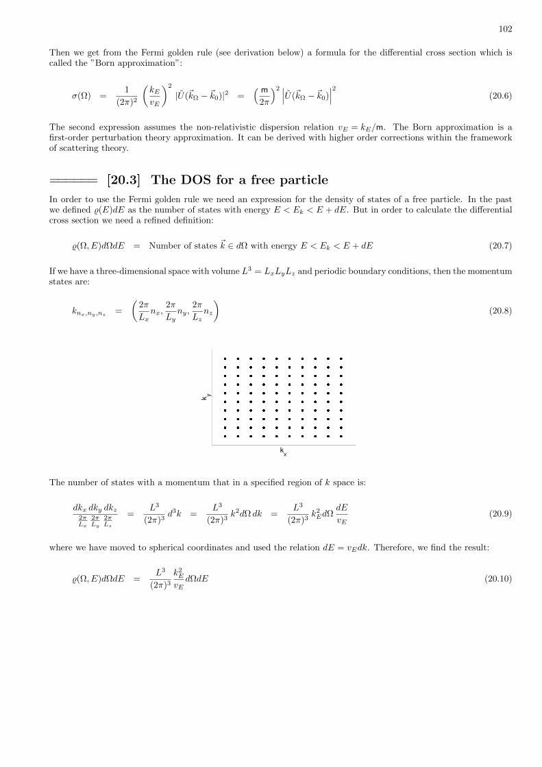
102

Then we get from the Fermi golden rule (see derivation below) a formula for the differential cross section which iscalled the ”Born approximation”:

σ(Ω) =1

(2π)2

(kEvE

)2

|U(~kΩ − ~k0)|2 =( m

2π

)2 ∣∣∣U(~kΩ − ~k0)∣∣∣2 (20.6)

The second expression assumes the non-relativistic dispersion relation vE = kE/m. The Born approximation is afirst-order perturbation theory approximation. It can be derived with higher order corrections within the frameworkof scattering theory.

====== [20.3] The DOS for a free particle

In order to use the Fermi golden rule we need an expression for the density of states of a free particle. In the pastwe defined %(E)dE as the number of states with energy E < Ek < E + dE. But in order to calculate the differentialcross section we need a refined definition:

%(Ω, E)dΩdE = Number of states ~k ∈ dΩ with energy E < Ek < E + dE (20.7)

If we have a three-dimensional space with volume L3 = LxLyLz and periodic boundary conditions, then the momentumstates are:

knx,ny,nz =

(2π

Lxnx,

2π

Lyny,

2π

Lznz

)(20.8)

kx

k y

The number of states with a momentum that in a specified region of k space is:

dkx dky dkz2πLx

2πLy

2πLz

=L3

(2π)3d3k =

L3

(2π)3k2dΩ dk =

L3

(2π)3k2EdΩ

dE

vE(20.9)

where we have moved to spherical coordinates and used the relation dE = vEdk. Therefore, we find the result:

%(Ω, E)dΩdE =L3

(2π)3

k2E

vEdΩdE (20.10)

103

====== [20.4] Derivation of the Born formula

Let us assume that we have a flux of particles that are moving in a box with periodic boundary conditions in thez direction. As a result of the presence of the scatterer there are transitions to other momentum states (i.e. to otherdirections of motion). According to the Fermi golden rule the transition rate is:

Γ(k ∈ dΩ|k0) = 2π [%(Ω, E)dΩ] |UkΩ,k0|2 (20.11)

By comparing with the definition of a cross section we get the formula:

σ(Ω) =2π

vEL3 %(Ω, E) |UkΩ,k0 |2 (20.12)

We notice that the matrix elements of the scattering potential are:

〈~k|U(r)| ~k0〉 =

∫d3x

L3e−ik·rU(r) eik0·r =

1

L3

∫U(r) e−i(k−k0)·rd3r =

1

L3U(k − k0) (20.13)

By substituting this expression and using the result for the density of states we get the Born formula.

====== [20.5] Scattering by a spherically symmetric potential

In order to use the Born formula in practice we define our system of coordinates as follows: the incident wavepropagates in the z direction, and the scattering direction is Ω = (θΩ, ϕΩ). The difference between the k of the

scattered wave and the k0 of the incident wave is ~q = ~k − ~k0. Next we have to calculate U(q) which is the Fouriertransform of U(r). If the potential is spherically symmetric we can use a rotated coordinate system for the calculationof the Fourier transform integral. Namely, we can use spherical coordinates such that θ = 0 is the direction of ~q.Consequently

U(q) =

∫ ∫ ∫U(r)e−iqr cos(θ)dϕd cos(θ)r2dr = 4π

∫ ∞0

U(r) sinc(qr) r2dr (20.14)

where the angular integration has been done using

∫ 1

−1

e−iλsds =

[e−iλs

−iλ

]1

−1

=eiλ − e−iλ

iλ=

2 sin(λ)

λ= 2sinc(λ) (20.15)

As an example consider U(r) = 1/r, for which we get U(q) = 4π/q2 (Rutherford formula).Next, we can go on calculating the total cross section:

σtotal =

∫ ∫σ(Ω)dΩ =

1

(2π)2

(kEvE

)2 ∫ π

0

|U(q)|2 2π sin θΩdθΩ (20.16)

We note that by simple trigonometry:

q = 2kE sin

(θΩ

2

); dq = kE cos

(θΩ

2

)dθΩ ; sin θΩdθΩ =

qdq

k2E

(20.17)

Hence we can write the integral of the cross section as:

σtotal =1

2πv2E

∫ 2kE

0

|U(q)|2qdq (20.18)

104

[21] Dynamics in the adiabatic picture

====== [21.1] The notion of adiabaticity

Consider a particle in a one dimensional box with infinite walls. We now move the wall. What happens to the particle?Let us assume that the particle has been prepared in a certain level. It turns out that if the wall is displaced slowly,the particle stays in the same level. This is called the ”adiabatic approximation”. We notice that staying in the sameenergy level means that the state of the particle changes! If the wall is moved very fast then the state of the particledoes not have time to change. This is called the ”sudden approximation”. In the latter case the final state (after thedisplacement of the wall) is not an eigenstate of the (new) Hamiltonian. After a sudden displacement of the wall, theparticle has to ”ergodize” its state inside the box.

The fact that the energy of the particle decreases when we move the wall outwards, means that the particle is doingwork. If the wall is displaced adiabatically, and then displaced back to its original location, then there is no net workdone. In such case we say that the process is reversible. But if the displacement of the wall is not adiabatically slow,the particle makes transitions to other energy levels. This scattering to other energy levels is in general irreversible.

In the problem that we have considered above, the parameter X that we change is the length L of the box. ThereforeV = X is the velocity at which the wall (or the ”piston”) is displaced. In other problems X could be any field. An

important example is a particle in a ring where X = Φ is the magnetic flux through the ring, and EMF = −X is theelectro motive force (by Faraday law). In problems of this type, the change in the parameter X can be very large,so we cannot use standard perturbation theory to analyze the evolution in time. Therefore, we would like to findanother way to write Schrodinger’s equation, so that X is the small parameter.

====== [21.2] The Schrodinger equation in the adiabatic basis

We assume that we have Hamiltonian H(Q, P ;X) that depends on a parameter X. The adiabatic states are theeigenstates of the instantaneous Hamiltonian:

H(X) |n(X)〉 = En(X) |n(X)〉 (21.1)

It is natural in such problems to work with the adiabatic basis and not with a fixed basis. We write the state of thesystem as:

|Ψ〉 =∑n

an(t) |n(X(t))〉 , an(t) ≡ 〈n(X(t))|Ψ(t)〉 (21.2)

If we prepare the particle in the energy level n0 and change X in adiabatically, then we shall see that |an(t)|2 ≈ δn,n0

at later times. We shall find a slowness condition for the validity of this approximation. Our starting point is theSchrodinger’s equation

dΨ

dt= −iH(x, p;X(t)) Ψ (21.3)

from which we get:

dandt

=

⟨n∣∣∣ ddt

Ψ

⟩+

⟨d

dtn∣∣∣Ψ⟩ = −i

⟨n∣∣∣Hψ⟩+

∑m

⟨d

dtn∣∣∣m⟩⟨m∣∣∣Ψ⟩ (21.4)

= −iEnan + X∑m

⟨∂

∂Xn∣∣∣m⟩ am ≡ −iEnan + iX

∑m

Anmam (21.5)

We conclude that in the adiabatic basis the effective Hamiltonian acquires an additional term, namely H 7→ H− XA.As an example consider the case where X is the position of a box that confine a particle, then we get in the movingframe H = H− Xp. See additional remark at the conclusion of the next sub-section.

105

====== [21.3] The calculation of Anm

Before we make further progress we would like to dwell on the calculation of the perturbation matrix Anm. First ofall we notice that for any X

⟨n∣∣∣m⟩ = δnm ;

∂

∂X

⟨n∣∣∣m⟩ = 0 ;

⟨∂

∂Xn∣∣∣m⟩+

⟨n∣∣∣ ∂∂X

m

⟩= 0 (21.6)

Which means that 〈∂n|m〉 is anti-Hermitian, and therefore −i 〈∂n|m〉 is Hermitian. If follows that

Anm = −i⟨

∂

∂Xn

∣∣∣∣m⟩ = i

⟨n

∣∣∣∣ ∂∂Xm

⟩= i

⟨n

∣∣∣∣T † ∂T∂X∣∣∣∣m⟩ (21.7)

where T (X) is the transformation to the moving frame, namely, |n(X)〉 = T (X) |n(0)〉. For the diagonal elements weuse the notation

An(X) = Ann = i

⟨n∣∣∣ ∂∂X

n

⟩(21.8)

With regard to the off-diagonal elements one observes that

Anm =−iVnmEn − Em

, Vnm ≡(∂H∂X

)nm

(21.9)

This is a very practical formula. Its proof is based on the following:

⟨n∣∣∣H∣∣∣m⟩ = 0 for n 6= m, for any X (21.10)

;∂

∂X

⟨n∣∣∣H∣∣∣m⟩ = 0

;⟨

∂

∂Xn∣∣∣H∣∣∣m⟩+

⟨n∣∣∣ ∂∂XH∣∣∣m⟩+

⟨n∣∣∣H∣∣∣ ∂

∂Xm

⟩= 0

; Em

⟨∂

∂Xn∣∣∣m⟩+ Vnm + En

⟨n∣∣∣ ∂∂X

m

⟩= 0

It should be noticed that the Hamiltonian in the adibatic basis can be regarded as the transformed Hamiltonian in amoving frame. Namely we have in fact re-derived the following result:

H = T †HT − iT † ∂T∂t

(21.11)

See lecture “Transformations and invariance” for further discussion. The second term (our ”A”) is simply the generatorof the transformation to the moving frame.

====== [21.4] The adiabatic condition

We found that in the adiabatic basis the Schrodinger’s equation takes the form

dandt

= −iEnan + iX∑m

Anmam ≡ −i(En − XAn)an − i∑m

Wnmam (21.12)

106

For sake of analysis we separated above the diagonal part of the perturbation. We use the simplified notationAn = Ann, and packed the off-diagonal elements into the matrix Wnm = −XAnm, whose diagonal elements are zero.It should be noticed that the strength of the perturbation in this representation is determined by the rate X and notby the amplitude of the driving.

Let us write again the Schrodinger equation in the adiabatic basis, with the substitution of the explicit expressionthat we have derived for the perturbation Wnm,

dandt

= −i(En − XAn)an + X∑m(6=n)

(Vnm

En − Em

)am (21.13)

If X is small enough, the perturbation matrix W is not able to induce transitions between levels, and we get theadiabatic approximation |an(t)|2 ≈ const. This means that the probability distribution does not change with time.In particular, if the particle is prepared in level n, then is stays in this level all the time.

From the discussion of first-order perturbation theory we know that we can neglect the coupling between two differentenergy levels if the absolute value of the matrix element is smaller compared with the energy difference between thelevels. Assuming that all the matrix elements are comparable the main danger to the adiabaticity are transitions toneighboring levels. Therefore the adiabatic condition is |W | ∆ or

X ∆2

~σ(21.14)

where σ is the estimate for the matrix element Vnm that couples neighbouring levels.

An example is in order. Consider a particle in a box of length L. The wall is displaced at a velocity X. Given that theenergy of the particle is E we recall that the energy level spacing is ∆ = (π/L)vE , while the coupling of neighbouringlevels, based on a formula that we derive in the Hard Walls subsection (p.188), is

σ =1

mLk2n =

1

mL(mvE)2 =

1

Lmv2

E (21.15)

It follows that the adiabatic condition is

X ~mL

(21.16)

Note that the result does not depend on E. This is not the typical case. In typical cases the density of states increaseswith energy, and consequently it becomes more difficult to satisfy the adiabatic condition.

It is worth pointing out that in the classical framework the adiabatic condition for a moving wall is X vE . Ifthe classical condition is violated the sudden approximation applies. If the classical condition is obeyed, but notthe quantum adiabatic condition, the dynamics is semi-classical. Namely, in each collision with the moving wall thechange of energy is ∆cl = 2mvEX. In the semi-classical regime the energy changes in steps ∆cl that are larger than ∆.This gives just the opposite condition to quantum adibaticity. For more details see [arXiv:cond-mat/0605591].

====== [21.5] The zero order adiabatic approximation

Assuming we can ignore the coupling between different levels, the adiabatic equation becomes

dandt

= −i(En − XAn)an (21.17)

And its solution is:

an(t) = eiΦn(t) an(0) (21.18)

107

where the accumulated phase is

Φn(t) =

∫ t

0

(−En + XAn

)dt′ = −

∫ t

0

Endt′ +

∫ X(t)

X(0)

An(X ′)dX ′ (21.19)

As already observed the probability |an(t)|2 to be in a specific energy level does not change in time. This is theadiabatic approximation. But it is interesting to look at the phase that the particle accumulates. Apart fromthe dynamical phase, the particle also accumulates a geometrical phase. An interesting case is when we severalparameters in a cyclic manner. In this case, just as in the Aharonov-Bohm effect, the “geometrical phase” is regardedas “topological phase” or “Berry phase”

ΦBerry ≡∮An(X) dX (21.20)

In fact, the Aharonov-Bohm effect can be viewed as a special case of the topological effect that has been explainedabove. In order to discuss further topological effects we have to generalize the derivation of the adiabatic equation.This will be done in the next lecture.

====== [21.6] Beyond the adiabatic approximation

Here we assume that we deal with one-parameter driving, accordingly the An can be gauged away, and the Φn issimply the integral over En. We can handle the adiabatic Hamiltonian within the framework of an “interactionpicture”, meaning that we substitute

an(t) = cn(t) eiΦn(t) (21.21)

hence getting the equation

dcndt

= X∑m(6=n)

VnmEn − Em

e−i(Φn−Φm) cm (21.22)

Note the implicit time dependence of the energies and the matrix elements, due to their parametric dependence onX = X(t). The leading order evaluation of the non-adiabatic transition probability is

Pt(n|m) =

∣∣∣∣∫ t

0

VnmEn − Em

e−i(Φn−Φm) Xdt

∣∣∣∣2 (21.23)

It is illuminating to consider a constant rate process X = const (>0) and use dX rather than dt integration. Thenthe above expression takes the following schematic form:

Pt =

∣∣∣∣∣∫ X2

X1

dX

g(X)exp

[− i

Xφ(X)

]∣∣∣∣∣2

∼ e−const/X (21.24)

The approximation is based on the assumption that the integral is dominated by a single complex pole where g(X) = 0.For the simplest example of such calculation see the Landau-Zener dynamics subsection, where we present the analysisof the non-adiabatic two-level crossing.

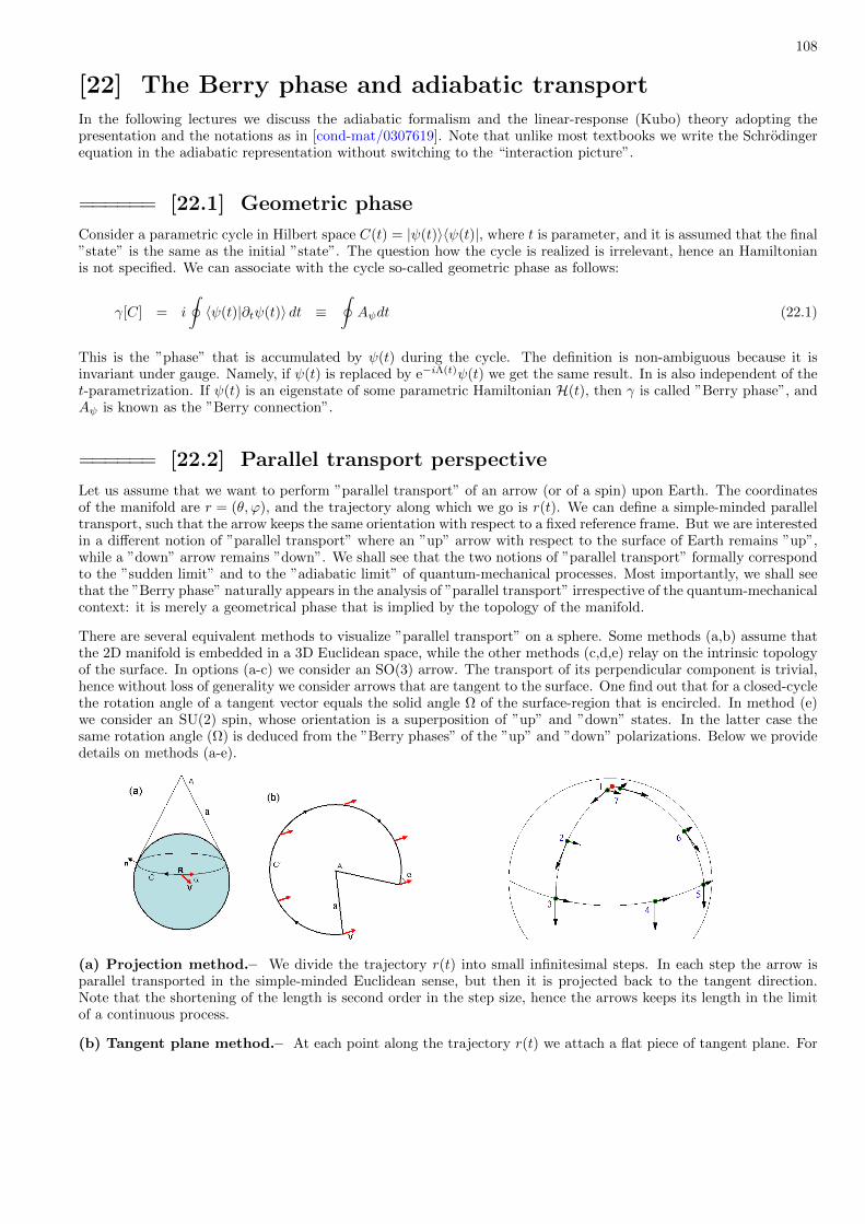
108

[22] The Berry phase and adiabatic transportIn the following lectures we discuss the adiabatic formalism and the linear-response (Kubo) theory adopting thepresentation and the notations as in [cond-mat/0307619]. Note that unlike most textbooks we write the Schrodingerequation in the adiabatic representation without switching to the “interaction picture”.

====== [22.1] Geometric phase

Consider a parametric cycle in Hilbert space C(t) = |ψ(t)〉〈ψ(t)|, where t is parameter, and it is assumed that the final”state” is the same as the initial ”state”. The question how the cycle is realized is irrelevant, hence an Hamiltonianis not specified. We can associate with the cycle so-called geometric phase as follows:

γ[C] = i

∮〈ψ(t)|∂tψ(t)〉 dt ≡

∮Aψdt (22.1)

This is the ”phase” that is accumulated by ψ(t) during the cycle. The definition is non-ambiguous because it isinvariant under gauge. Namely, if ψ(t) is replaced by e−iΛ(t)ψ(t) we get the same result. In is also independent of thet-parametrization. If ψ(t) is an eigenstate of some parametric Hamiltonian H(t), then γ is called ”Berry phase”, andAψ is known as the ”Berry connection”.

====== [22.2] Parallel transport perspective

Let us assume that we want to perform ”parallel transport” of an arrow (or of a spin) upon Earth. The coordinatesof the manifold are r = (θ, ϕ), and the trajectory along which we go is r(t). We can define a simple-minded paralleltransport, such that the arrow keeps the same orientation with respect to a fixed reference frame. But we are interestedin a different notion of ”parallel transport” where an ”up” arrow with respect to the surface of Earth remains ”up”,while a ”down” arrow remains ”down”. We shall see that the two notions of ”parallel transport” formally correspondto the ”sudden limit” and to the ”adiabatic limit” of quantum-mechanical processes. Most importantly, we shall seethat the ”Berry phase” naturally appears in the analysis of ”parallel transport” irrespective of the quantum-mechanicalcontext: it is merely a geometrical phase that is implied by the topology of the manifold.

There are several equivalent methods to visualize ”parallel transport” on a sphere. Some methods (a,b) assume thatthe 2D manifold is embedded in a 3D Euclidean space, while the other methods (c,d,e) relay on the intrinsic topologyof the surface. In options (a-c) we consider an SO(3) arrow. The transport of its perpendicular component is trivial,hence without loss of generality we consider arrows that are tangent to the surface. One find out that for a closed-cyclethe rotation angle of a tangent vector equals the solid angle Ω of the surface-region that is encircled. In method (e)we consider an SU(2) spin, whose orientation is a superposition of ”up” and ”down” states. In the latter case thesame rotation angle (Ω) is deduced from the ”Berry phases” of the ”up” and ”down” polarizations. Below we providedetails on methods (a-e).

(a) Projection method.– We divide the trajectory r(t) into small infinitesimal steps. In each step the arrow isparallel transported in the simple-minded Euclidean sense, but then it is projected back to the tangent direction.Note that the shortening of the length is second order in the step size, hence the arrows keeps its length in the limitof a continuous process.

(b) Tangent plane method.– At each point along the trajectory r(t) we attach a flat piece of tangent plane. For

109

example, if we move along a line of constant latitude the union of all these pieces is a conical surface. This surfacecan be regarded as flat, and we can perform on it an Euclidean ”parallel transport”. See left panels of the figure[N.P.Ong website].

(c) Geodesic walk method.– We can always approximated r(t) as a sum of infinitesimal geodesic steps. In thecase of a sphere ”geodesic” means to go along a big circle. The law of ”parallel transport” is simple: the arrow shouldkeep fixed angle with the geodesic. See right panel of the figure [N.Manini website].

(d) Metric connection method.– To each point r = (x1, x2) on the surface we attach a set of ”unit vectors” withwhich a metric is associated:

−→e n = ∂nr =∂r

∂xn, gnm = 〈−→e n|−→e m〉 = 〈∂nr|∂mr〉 (22.2)

Then we can define so called ”connection”, that can be derived from the metric:

Γn,km = 〈−→e n|∂k−→e m〉 = 〈∂nr|∂k∂mr〉 =1

2[∂kgnm + ∂mgkn − ∂ngkm] (22.3)

The metric connection allows us to calculate full derivatives:

|v〉 =∑n

vn |−→e n〉 , Dk |v〉 =∑n

[∂kvn +

∑m

Γn,kmvm

]|−→e n〉 (22.4)

The construct D = ∂ + Γ is known as the ”covariant derivative”. It takes into account the explicit variation of thevector-components as well as the implicit parametric variation of the basis-vectors. We say that the vector v isparallel transported if Dv = 0. Accordingly Γ can be regarded as the generator of an orthogonal transformation thatpreservers the scalar product.

(e) Hermitian connection method.– We can repeat the formal derivation of the parallel transport law, consideringtransport of SU(2) spins instead of SO(3) arrows. To each point r = (x1, x2) on the surface we attach a set basisvectors |n(r)〉. For example:

|↑ (θ, ϕ)〉 =

(cos(θ/2)

eiϕ sin(θ/2)

), |↓ (θ, ϕ)〉 =

(sin(θ/2)

−eiϕ cos(θ/2)

)(22.5)

Then we can define an Hermitian connection, and an associate covariant derivative as follows:

Dk[simple minded parallel transport] = ∂k + 〈n(r)|∂km(r)〉 ≡ ∂k − iAknm (22.6)

The requirement Dψ = 0 defines a simple-minded parallel transport, corresponding to the sudden-approximation inthe quantum-dynamics context. We would like to define a different notion of ”parallel transport” that respects ”up”and ”down” relative to the surface. Therefore the ”connection” in the definition of the covariant derivative shouldbe modified. In a fixed-basis frame we can write D = ∂ − iΓ, while in the n-basis frame it should transforms into adiagonal matrix

Dk[parametric parallel transport] = ∂k − i[Γknm +Aknm

]≡ ∂k − iAknm (22.7)

where A = diagAn is a diagonal matrix in the n-representation. In the concluding paragraph of this section we

argue that An should be identified as the Berry connection, hence Aknm = δn,mAknm. Once this is established it follows

automatically that for a cyclic parallel transport process Cn(t) = |n(t)〉〈n(t)|, the transported |n〉 accumulates a phasethat equals γn = γ[Cn]. Consequently, if we start at r0 and go along a trajectory r(t) back to r0, then a tangent spinwill rotate as follows:

|↑ (r0)〉+ |↓ (r0)〉 ; eiγ↑[r] |↑ (r0)〉+ eiγ↓[r] |↓ (r0)〉 RotationAngle = −(γ↑ − γ↓) (22.8)

110

Specifically if we go along the constant θ latitude line, the connection is Aϕ↑ = −[sin(θ/2)]2, and one obtains γ↑ = −Ω/2,

where Ω = 2π[1− cos(θ)]. Similarly for a ”down” spin one obtains γ↓ = +Ω/2. Hence the expected result for therotation angle is recovered.

Natural hermitian connection.– To deduce the connection for an SO(3) arrow given the metric of the manifoldis easy. To deduce the connection for an SU(2) spin requires further reasoning. What we want is to have a paralleltransport law that preserves |n〉〈n|. This means that ”up” remains ”up” and ”down” remains ”down”. Namely|ψ(t)〉 = eiγn(t) |n(t)〉 should be qualified as a parallel-transport process, where γn(t) still has to be determined. Fromsuch transport law it follows that An = ∂tγn. We would like to argue that the proper determination of γn(t) impliesthat An is the Berry connection.

At first sight it seems that the problem is ill-defined, and that γn(t) can be chosen in an arbitrary way. Thenaive prescription would be γn(t) = 0. Clearly such prescription is gauge dependent: if we define a different basis|n(r)〉 = e−iΛn(r) |n(r)〉 we get a different rotation angle for a tangent vector. Even if we allow such gauge-dependentlaw of transport, still there is a problem. For a manifold with non-trivial topology (here it is a sphere) there is no wayto have a well-defined gauge globally. With our choice of gauge the n states at the SouthPole remains ambiguous.Any gauge requires the exclusion of at least one point from the sphere, which is like saying that we are not dealingwith a sphere...

The remedy for all this gauge-related complications is to define a parallel-transport law that does not depend onthe gauge. Saying it differently, we claim that there is a natural way to define a gauge-invariant connection, suchthat ”up” remains ”up” and ”down” remains ”down”. We first note that a change |δψ〉 = |ψ(t+dt)〉 − |ψ(t)〉 can bedecomposed into ”parallel” and ”transverse” components as follows:

|δψ〉‖ = |ψ〉 〈ψ|δψ〉 = −iAψ |ψ〉 (22.9)

|δψ〉⊥ = |δψ〉 − |ψ〉 〈ψ|δψ〉 = |δψ〉+ iAψ |ψ〉 (22.10)

Inspired by the “projection method” for constructing a parallel-transport process, the requirement for parallel trans-port becomes |δψ〉‖ = 0. Note that in the SO(3) treatment the projection was onto the tangent direction, while here

we are keeping the spin in the perpendicular (”parallel”) direction. We realize that |n(t)〉 is not a proper paralleltransport process. The remedy is to consider |ψ(t)〉 = eiγn(t) |n(t)〉 with ∂tγn = An(t), which is a gauge-invariant

prescription. This implies that A = diagAn is the hermitian connection.

====== [22.3] The Berry curvature

We consider a set of basis states 〈n(x)| that depend on a set of parameters x = (x1, x2, x3, ...). In the previous sectionwe have motivated the definition of the hermitian connection matrix

Ajnm(x) = i~⟨n(x)

∣∣∣ ∂∂xj

m(x)

⟩(22.11)

The hermiticity of the matrix can be deduced via differentiation by parts of ∂j〈n(x)|m(x)〉 = 0. Furthermore, fromdifferentiation by parts of ∂j〈n(x)|H|m(x)〉 = 0, we get for n 6= m the following expressions:

Ajnm(x) =i~

Em − En

⟨n

∣∣∣∣ ∂H∂xj∣∣∣∣m⟩ ≡ − i~F jnm

Em − En(22.12)

It should be realized that Ajnm is not gauge invariant. The effect of gauge transformation is

|n(x)〉 7→ e−iΛn(x)

~ |n(x)〉 (22.13)

Ajnm 7→ eiΛn−Λm

~ Ajnm + (∂jΛn)δnm

We now focus on the the diagonal elements Ajn ≡ Ajnn. These are real, and transform as Ajn 7→ Ajn+∂jΛn. Associated

111

with An(x) is the gauge invariant 2-form which is called the ”Berry curvature”:

Bkjn = ∂kAjn − ∂jAkn = −2~Im〈∂kn|∂jn〉 = −2

~Im∑m

AknmAjmn (22.14)

This can be written in abstract notation as B = ∂ ∧ A, and if not singular (see below) it has zero divergence(∂ ∧B = ∂ ∧ ∂ ∧A = 0). The derivation of the following identity is straightforward:

Bkjn = 2~∑m(6=n)

Im[FknmF jmn

](Em − En)2

(22.15)

From this expression it is evident that the sources of the divergenceless field Bn are located at point where it encountersa degeneracy with a neighbouring level. Also it is useful to notice that

∑Bn = 0, because the double summation

results in a real expression inside the Im[]. The Berry phase can be regarded as the ”flux” of B, namely,

γn =

∮An · dr =

xBn · ds (22.16)

Using the same argumentation as in the discussion of Dirac monopoles (see [here]) we deduce that

1

2π

Bn · ds = integer ≡ Chern number (22.17)

The mathematical digression below clarifies the analogy between B and the notion of magnetic field.

====== [22.4] Digression - Geometrical Forms

Geometrical forms are the “vector analysis” generalization of the length, area and volume concepts to any dimension.In Euclidean geometry with three dimensions the basis for the usual vector space is e1, e2, e3. These are called 1-forms.We can also define a basis for surface elements (2-forms) and volume (3-form).

e12 = e1 ∧ e2 e23 = e2 ∧ e3 e31 = e3 ∧ e1 e1 ∧ e2 ∧ e3 (22.18)

By definition e21 = −e12, and e1∧ e2∧ e3 = −e2∧ e1∧ e3 etc. There is a natural duality between 2-forms and 1-forms,namely e12 7→ e3 and e23 7→ e1 and e31 7→ e2. This duality between surface elements and 1-forms does not holdin Euclidean geometry of higher dimension. For example in 4 dimensions the surface elements (2-forms) constituteC2

4 = 6 dimensional space. In the latter case we have duality between the hyper-surface elements (3-forms) and the1-forms, which are both 4 dimensional spaces. There is of course the simplest example of Euclidean geometry in 2diemnsional space where 2-forms are regarded as either area or as volume and not as 1-form vectors. In general forN dimensional Euclidean geometry the k forms constitute a CkN dimensional vector space, and they are dual to the(N − k) forms. We can multiply 1-forms as follows:[∑

Aiei

]∧[∑

Biej

]=

∑i,j

AiAj ei ∧ ej =∑i<j

(AiAj −AjAi)ei ∧ ej (22.19)

Note that ei ∧ ei = Null. This leads to the practical formula for a wedge product

(A ∧B)ij = AiBj −AjBi (22.20)

Similarly we use the notation (∂ ∧ A)ij = ∂iAj − ∂jAi. Note that in 3 dimensional Euclidean geometry we have thefollowing association with conventional ”vector analysis” notations:

∂ ∧A 7→ ∇ ×A if A is a 1-forms (22.21)

∂ ∧B 7→ ∇ ·B if B is a 2-forms

112

The above identifications are implied by the following:

∂ = ∂1e1 + ∂1e2 + ∂1e3 (22.22)

A = A1e1 +A2e2 +A3e3

B = B12e12 +B23e23 +B31e31

We now introduce a more flexible notations. We regard any scalar function f(x) as a 0-form, and associate differentialquantities with 1-forms and 2-forms as follows:

wf = f(x) wA =

∑j

Ajdxj

≡ A · dr wB =

∑i<j

Bijdxi ∧ dxj

≡ B · ds (22.23)

we also use the notation d =∑j ∂jdxj for full differential. With this notation a relation like B = ∂ ∧A can be written

as wB = d ∧ wA. The Stokes integral theorem is conventionally written as

∮A · dr =

x∂ ∧A · ds (22.24)

This concerns 1-forms. The Divergence integral theorem concerns 2-forms. The generalized Stokes theorem relatesthe closed boundary integral over a k-form to an integral over a (k+1)-form within the interior. With the abovenotations it can be written as∮

wA =x

d ∧ wA (22.25)

where A is any k-form.

====== [22.5] Adiabatic evolution

The adiabatic equation is obtained from the Schrodinger equation by expanding the wavefunction in the x-dependentadiabatic basis:

d

dt|ψ〉 = − i

~H(x(t)) |ψ〉 (22.26)

|ψ〉 =∑n

an(t) |n(x(t))〉

dandt

= − i~Enan +

i

~∑m

∑j

xjAjnmam

We define the perturbation matrix as

Wnm = −∑j

xjAjnm for n 6= m (22.27)

and W jnm = 0 for n = m. Then the adiabatic equation can be re-written as follows:

dandt

= − i~

(En − xAn)an −i

~∑m

Wnmam (22.28)

113

If we neglect the perturbation W , then we get the strict adiabatic solution:

|ψ(t)〉 = e− i

~

(∫ t0En(x(t′))dt′−

∫ x(t)

x(0)An(x)·dx

)|n(x(t))〉 (22.29)

The time dependence of this solution is exclusively via the x dependence of the basis states. On top, due to An(x)we have the so called geometric phase. This can be gauged away unless we consider a closed cycle. For a closed cycle,

the gauge invariant phase 1~∮~A · ~dx is called the Berry phase.

With the above zero-order solution we can obtain the following result:

〈Fk〉 =

⟨ψ(t)

∣∣∣∣− ∂H∂xk∣∣∣∣ψ(t)

⟩= − ∂

∂xk〈n(x)| H(x) |n(x)〉 (22.30)

In the standard examples this corresponds to a conservative force or to a persistent current. From now on we ignorethis trivial contribution to 〈Fk〉, and look for the a first order contribution.

====== [22.6] Adiabatic Transport

For linear driving (unlike the case of a cycle) the An(x) field can be gauged away. Assuming further that the adiabaticequation can be treated as parameter independent (that means disregarding the dependence of En and W on x) onerealizes that the Schrodinger equation in the adiabatic basis possesses stationary solutions. To first order these are:

|ψ(t)〉 = |n〉+∑m(6=n)

Wmn

En − Em|m〉 (22.31)

Note that in a fixed-basis representation the above stationary solution is in fact time-dependent. Hence the explicitnotations |n(x(t))〉 and |m(x(t))〉 are possibly more appropriate.

With the above solution we can write 〈Fk〉 as a sum of zero order and first order contributions. From now on weignore the zero order contribution, but keep the first order contribution:

〈Fk〉 = −∑m(6=n)

Wmn

En − Em

⟨n∣∣∣ ∂H∂xk

∣∣∣m⟩+ CC =∑j

(i∑m

AknmAjmn + CC

)xj = −

∑j

Bkjn xj (22.32)

For a general stationary preparation, either pure or mixed, one obtains

〈Fk〉 = −∑j

Gkj xj (22.33)

with

Gkj =∑n

f(En) Bkjn (22.34)

where f(En) are weighting factors, with the normalization∑n f(En) = 1. For a pure state preparation f(En)

distinguishes only one state n, while for a canonical preparation f(En) ∝ e−En/T , where T is the temperature.For a many-body system of non-interacting particles f(En) is re-interpreted as the occupation function, so that∑n f(En) = N is the total number of particles.

Thus we see that the assumption of a stationary first-order solution leads to a non-dissipative (antisymmetric) con-ductance matrix. This is known as either ”adiabatic transport” or ”geometric magnetism”. In the next lecture weare going to see that ”adiabatic transport” is in fact a special limit of the Kubo formula.

114

[23] Linear response theory and the Kubo formula

====== [23.1] Linear Response Theory

We assume that the Hamiltonian depends on several parameters, say three parameters:

H = H(~r, ~p; x1(t), x2(t), x3(t)) (23.1)

and we define generalized forces

Fk = − ∂H∂xk

(23.2)

Linear response means that

〈Fk〉t =∑j

∫ ∞−∞

αkj(t− t′) δxj(t′)dt′ (23.3)

where αkj(τ) = 0 for τ < 0. The expression for the response Kernel is known as the Kubo formula:

αkj(τ) = Θ(τ)i

~〈[Fk(τ),F j(0)]〉0 (23.4)

where the average is taken with the assumed zero order stationary solution. Before we present the standard derivationof this result we would like to illuminate the DC limit of this formula, and to further explain the adiabatic limit thatwas discussed in the previous section.

====== [23.2] Susceptibility and DC Conductance

The Fourier transform of αkj(τ) is the generalized susceptibility χkj(ω). Hence

[〈Fk〉]ω =∑j

χkj0 (ω)[xj ]ω −∑j

µkj(ω)[xj ]ω (23.5)

where the dissipation coefficient is defined as

µkj(ω) =Im[χkj(ω)]

ω=

∫ ∞0

αkj(τ)sin(ωτ)

ωdτ (23.6)

In the ”DC limit” (ω → 0) it is natural to define the generalized conductance matrix:

Gkj = µkj(ω ∼ 0) = limω→0

Im[χkj(ω)]

ω=

∫ ∞0

αkj(τ)τdτ (23.7)

Consequently the non-conservative part of the response can be written as a generalized Ohm law.

〈Fk〉 = −∑j

Gkj xj (23.8)

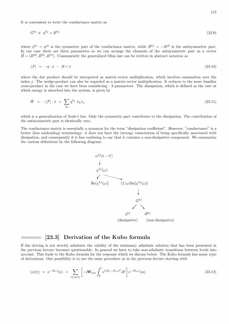
115

It is convenient to write the conductance matrix as

Gkj ≡ ηkj +Bkj (23.9)

where ηkj = ηjk is the symmetric part of the conductance matrix, while Bkj = −Bjk is the antisymmetric part.In our case there are three parameters so we can arrange the elements of the antisymmetric part as a vector~B = (B23, B31, B12). Consequently the generalized Ohm law can be written in abstract notation as

〈F〉 = −η · x − B ∧ x (23.10)

where the dot product should be interpreted as matrix-vector multiplication, which involves summation over theindex j. The wedge-product can also be regarded as a matrix-vector multiplication. It reduces to the more familiarcross-product in the case we have been considering - 3 parameters. The dissipation, which is defined as the rate atwhich energy is absorbed into the system, is given by

W = −〈F〉 · x =∑kj

ηkj xkxj (23.11)

which is a generalization of Joule’s law. Only the symmetric part contributes to the dissipation. The contribution ofthe antisymmetric part is identically zero.

The conductance matrix is essentially a synonym for the term ”dissipation coefficient”. However, ”conductance” is abetter (less misleading) terminology: it does not have the (wrong) connotation of being specifically associated withdissipation, and consequently it is less confusing to say that it contains a non-dissipative component. We summarizethe various definitions by the following diagram:

?

XXXXXXz

?

@@R

αkj(t− t′)

χkj(ω)

Re[χkj(ω)] (1/ω)Im[χkj(ω)]

ηkj Bkj

(non-dissipative)

Gkj

(dissipative)

====== [23.3] Derivation of the Kubo formula

If the driving is not strictly adiabatic the validity of the stationary adiabatic solution that has been presented inthe previous lecture becomes questionable. In general we have to take non-adiabatic transitions between levels intoaccount. This leads to the Kubo formula for the response which we discuss below. The Kubo formula has many typeof derivations. One possibility is to use the same procedure as in the previous lecture starting with

|ψ(t)〉 = e−iEnt|n〉 +∑m(6=n)

[−iWmn

∫ t

0

ei(En−Em)t′dt′]

e−iEmt|m〉 (23.12)

116

We shall not expand further on this way of derivation, which becomes quite subtle once we go beyond the stationaryadiabatic approximation. A one line derivation of the Kubo formula is based on the interaction picture, and ispresented in a dedicted section There are various different looking derivations of the Kubo formula that highlight thequantum-to-classical correspondence and/or the limitations of this formula. The advantage of the derivation below isthat it also allows some extensions within the framework of a master equation approach that takes the environmentinto account.

For notational simplicity we write the Hamiltonian as

H = H0 − f(t)V (23.13)

We assume that the system, in the absence of driving, is prepared in a stationary state ρ0. In the presence of drivingwe look for a first order solution ρ(t) = ρ0 + ρ(t). The equation for ρ(t) is:

∂ρ(t)

∂t≈ −i[H0, ρ(t)] + if(t)[V, ρ0] (23.14)

Next we use the substitution ρ(t) = U0(t)˜ρ(t)U0(t)−1, where U0(t) is the evolution operator which is generated byH0. Thus we eliminate from the equation the zero order term:

∂ ˜ρ(t)

∂t≈ if(t)[U0(t)−1V U0(t), ρ0] (23.15)

The solution of the latter equation is straightforward and leads to

ρ(t) ≈ ρ0 +

∫ t

i [V (−(t−t′)), ρ0] f(t′)dt′ (23.16)

where we use the common notation V (τ) = U0(τ)−1V U0(τ).

Consider now the time dependence of the expectation value 〈F〉t = trace(Fρ(t)) of an observable. Disregarding thezero order contribution, the first order expression is

〈F〉t ≈∫ t

i trace (F [V (−(t−t′)), ρ0]) f(t′)dt′ =

∫ t

α(t− t′) f(t′)dt′

where the response kernel α(τ) is defined for τ > 0 as

α(τ) = i trace (F [V (−τ), ρ0]) = i trace ([F , V (−τ)]ρ0) = i〈[F , V (−τ)]〉 = i〈[F(τ), V ]〉 (23.17)

where we have used the cyclic property of the trace operation; the stationarity U0ρ0U−10 = ρ0 of the unperturbed

state; and the notation F(τ) = U0(τ)−1FU0(τ).

117

[24] The Born-Oppenheimer pictureWe now consider a more complicated problem, where x becomes a dynamical variable. The standard basis for therepresentation of the composite system is |x,Q〉 = |x〉 ⊗ |Q〉. We assume a total Hamiltonian of the form

Htotal =1

2m

∑j

p2j +H(Q,P ;x)− f(t)V (Q) (24.1)

Rather than using the standard basis, we can use the Born-Oppenheimer basis |x, n(x)〉 = |x〉 ⊗ |n(x)〉. Accordinglythe state of the combined system is represented by the wavefunction Ψn(x), namely

|Ψ〉 =∑n,x

Ψn(x) |x, n(x)〉 (24.2)

The matrix elements of H are

〈x, n(x)|H|x0,m(x0)〉 = δ(x− x0)× δnmEn(x) (24.3)

The matrix elements of V (Q) are

〈x, n(x)|V (Q)|x0,m(x0)〉 = δ(x− x0)× Vnm(x) (24.4)

The matrix elements of p are

〈x, n(x)|pj |x0,m(x0)〉 = (−i∂jδ(x−x0))× 〈n(x)|m(x0)〉

The latter can be manipulated ”by parts” leading to

〈x, n(x)|pj |x0,m(x0)〉 = −i∂jδ(x− x0)δnm − δ(x− x0)Ajnm(x) (24.5)

This can be summarized by saying that the operation of pj on a wavefunction is like the differential operator−i∂j −Ajnm(x). Thus in the Born-Oppenheimer basis the total Hamiltonian takes the form

Htotal =1

2m

∑j

(pj −Ajnm(x))2 + δnmEn(x)− f(t)Vnm(x) (24.6)

Assuming that the system is prepared in energy level n, and disregarding the effect of A and V , the adiabatic motion ofx is determined by the effective potential En(x). This is the standard approximation in studies of diatomic molecules,where x is the distance between the nuclei. If we treat the slow motion as classical, then the interaction with A canbe written as

H(1)interaction = −

∑j

xjAjnm(x) (24.7)

This brings us back to the theory of driven systems as discussed in previous sections. The other interaction that caninduce transitions between levels is

H(2)interaction = −f(t)Vnm(x) (24.8)

The analysis of molecular ”wavepacket dynamics” is based on this picture.

118

The Green function approach

[25] The propagator and Feynman path integral

====== [25.1] The propgator

The evolution of a quantum mechanical system is described by a unitary operator

|Ψ(t)〉 = U(t, t0) |Ψ(t0)〉 (25.1)

The Hamiltonian is defined by writing the infinitesimal evolution as

U(t+ dt, t) = 1− idtH(t) (25.2)

This expression has an imaginary i in order to make H a Hermitian matrix. If we want to describe continuousevolution we can ”break” the time interval into N infinitesimal steps:

U(t, t0) = (1− idtNH) . . . (1− idt2H)(1− idt1H) ≡ T e−i∫ tt0H(t′)dt′

(25.3)

For a time independent Hamiltonian we get simply U(t) = e−itH because of the identity eAeB = eA+B if [A,B] = 0.

If we consider a particle and use the standard position representation then the unitary operator is represented by amatrix U(x|x0). The time interval [t0, t] is implicit. We alway assume that t > t0. Later it would be convenient todefine the propagator as U(x|x0) for t > t0 and as zero otherwise. The reason for this convention is related to theformalism that we are going to introduce later on.

====== [25.2] The Propagator for a free particle

Consider a free particle in one dimension. Let us find the propagator using a direct calculation. The hamiltonian is:

H =p2

2m(25.4)

As long as the Hamiltonian has a quadratic form, the answer will be a Gaussian kernel:

U(x|x0) =⟨x∣∣∣e−i t2mp2

∣∣∣x0

⟩=( m

2πit

) 12

eim2t (x−x0)2

(25.5)

We note that in the case of a harmonic oscillator

H =p2

2m+

1

2mΩ2x2 (25.6)

The propagator is

U(x|x0) =

(mΩ

2πi sin Ωt

) 12

eimΩ

2 sin Ωt [cos Ωt(x2+x20)−2xx0] (25.7)

If we take t→ 0 then U → 1, and therefore U(x|x0)→ δ(x− x0).

119

The derivation of the expression for the propagator in the case of a free particle goes as follows. For clarity we useunits such that m = 1:

〈x|e−ı 12 tp

2

|x0〉 =∑k

〈x|k〉e−ı 12 tk

2

〈k|x0〉 =

∫dk

2πe−ı

12 tk

2+ik(x−x0) (25.8)

This is formally an inverse FT of a Gaussian. One obtains the desired result, which is formally a Gaussian that hasan imaginary variance σ2 = it. We note that we can write the result in the form

〈x|e−ı 12 tp

2

|x0〉 =1√2πıt

eı(x−x0)2

2t =1√2πıt

[cos

1

2t(x− x0)2 + ı sin

1

2t(x− x0)2

](25.9)

If t → 0 we should get a delta function. This is implied by the FT, but it would be nice to verify this statementdirectly. Namely we have to show that in this limit we get a narrow function whose ”area” is unity. For this purposewe use identity

∫cos r2 . . . dr =

∫cosu

2√u. . . du (25.10)

and a similar expression in case of sin function. Then we recall the elementary integrals

∫ ∞0

sinu√udu =

∫ ∞0

cosu√udu =

√π

2(25.11)

Thus the ”area” of the two terms in the square brackets is proportional to (1 + i)/√

2 which cancels the√i of the

prefactor.

====== [25.3] Feynman Path Integrals

How can we find the propagator U(x|x0) for the general Hamiltonian H = p2

2m +V (x)? The idea is to write 〈x|e−ıtH|x0〉as a convolution of small time steps:

〈x|e−ıtH|x0〉 =∑

x1,x2,...xN−1

〈x|e−ıδtNH|xN−1〉 . . . 〈x2|e−ıδt2H|x1〉〈x1|e−ıδt1H|x0〉 (25.12)

Now we have to find the propagator for each infinitesimal step. At first sight it looks as if we just complicated thecalculation. But then we recall that for infinitesimal operations we have:

eεA+εB ≈ eεAeεB ≈ eεBeεA for any A and B (25.13)

This is because the higher order correction can be made as small as we want. So we write

〈xj |e−ıδt(p2

2m +V (x))|xj−1〉 ≈ 〈xj |e−ıδtV (x))e−ıδtp2

2m |xj−1〉 ≈ (m

2πıdtj)

12 eı m2dtj

(xj−xj−1)2−dtjV (xj)(25.14)

and get:

U(x|x0) =

∫dx1dx2 . . . dxN−1(

m

2πıdt)N2 eiA[x] ≡

∫d[x] eiA[x] (25.15)

120

where A[x] is called the action.

A[x] =

N−1∑j=1

[ m

2dt(xj − xj−1)2 − dtV (x)

]=

∫(1

2mx2 − V (x))dt =

∫L(x, x)dt (25.16)

More generally, if we include the vector potential in the Hamiltonian, then we get the Lagrangian

L(x, x) =1

2mx2 − V (x) +A(x)x (25.17)

leading to:

A[x] =

∫(1

2mx2 − V (x))dt+

∫A(x) · dx (25.18)

====== [25.4] Stationary Point Approximation

The Stationary Point Approximation is an estimate for an integral of the form∫

eıA(x)dx. The main contribution tothe integral comes from the point x = x, called a stationary point, where A′(x) = 0. We expand the function A(x)near the stationary point:

A(x) = A(x) +1

2A′′(x)(x− x)2 + . . . (25.19)

Leading to

∫eıA(x)dx ≈ eıA(x)

∫eı

12A

”(x)(x−x)2

dx =

√i2π

A”(x)eıA(x) (25.20)

where the exponential term is a leading order term, and the prefactor is an ”algebraic decoration”.

The generalization of this method to multi-dimensional integration over d[x] is immediate. The stationary point isin fact the trajectory for which the first order variation is zero (δA = 0). This leads to Lagrange equation, whichimplies that the ”stationary point” is in fact the classical trajectory. Consequently we get the so called semiclassical(Van-Vleck) approximation:

U(x|x0) =

∫d[x] eiA[x] ≈

∑cl

(1

i2π~

)d/2 ∣∣∣∣det

(− ∂

2Acl∂x∂x0

)∣∣∣∣1/2 eiAcl(x,x0)−i(π/2)νcl (25.21)

where d is the number of degrees of freedom, and

Acl(x, x0) ≡ A[xcl] (25.22)

is the action of the classical trajectory as a function of the two end points. In d dimensions the associated determinantis d×d. The Morse-Maslov index νcl counts the number of conjugate points along the classical trajectory. If the timeis short it equals zero and then both this index and the absolute value that enclosed the determinant can be omitted.Otherwise the recipe for the determination of the Morse index is as follows: The linearized equation of motion forx(t) = xcl(t) + δx(t) is

mδx+ V ′′(xcl)δx = 0 (25.23)

121

A conjugate point (in time) is defined as the time when the linearized equation has a non-trivial solution. Withthis rule we expect that in case of a reflection from a wall, the Morse index is +1 for each collision. This is correctfor “soft” wall. In case of “hard” wall the standard semiclassical result for νcl breaks down, and the correct resultturns out to be +2 for each collision. The latter rule is implied by the Dirichlet boundary conditions. Note, thatit would be +0 in the case of Neumann boundary conditions. The Van-Vleck semiclassical approximation is exactfor quadratic Hamiltonians because the ”stationary phase integral” is exact if there are no higher order terms in theTaylor expansion.

Let us compute again U(x|x0) for a free particle, this time using the Van-Vleck expression: The action A[x] for thefree particle is

A[x] =

∫ t

0

1

2mx2dt′. (25.24)

Given the end points we find the classical path

xcl = x0 +x− x0

tt′ (25.25)

and hence

Acl(x, x0) =

∫ t

0

1

2m(

x− x0

t)2dt′ =

m

2t(x− x0)2. (25.26)

We also observe that

− ∂2Acl

∂x∂x0=

m

t(25.27)

which leads to the exact result. The big advantage of this procedure emerges clearly once we try to derive the moregeneral expression in case of a harmonic oscillator.

122

[26] The resolvent and the Green function

====== [26.1] The resolvent

The resolvent is defined in the complex plane as

G(z) =1

z −H(26.1)

In case of a bounded system it has poles at the eigenvalues. We postpone for later the discussion of unboundedsystems. It is possibly more illuminating to look on the matrix elements of the resolvent

G(x|x0) = 〈x|G(z)|x0〉 =∑n

ψn(x)ψn(x0)∗

z − En≡∑n

qnz − En

(26.2)

where ψn(x) = 〈x|n〉 are the eigenstates of the Hamiltonian. If we fix x and x0 and regard this expression as a functionof z this is formally the complex representation of an electric field in a two dimensional electrostatic problem.

We can look on G(x|x0), with fixed z = E and x0, as a wavefunction in the variable x. We see that G(x|x0) is asuperposition of eigenstates. If we operate on it with (E − H) the coefficients of this superposition are multipliedby (E − Ek), and because of the completeness of the basis we get δ(x − x0). This means that G(x|x0) satisfies theSchrodinger equation with the complex energy E and with an added source at x = x0. Namely,

(E −H)G(x|x0) = δ(x− x0) (26.3)

This is simply the standard representation of the equation (z −H)G = 1 which defines the matrix inversionG = 1/(z −H). The wavefunction G(x|x0) should satisfy that appropriate boundary conditions. If we deal witha particle in a box this means Dirichlet boundary conditions. In the case of an unbounded system the issue ofboundary conditions deserves further discussion (see later).

The importance of the Green functions comes from its Fourier transform relation to the propagator. Namely,

FT[

Θ(t)e−γt U(t)]

= iG(ω + iγ) (26.4)

where Θ(t) is the step function, Θ(t)U(t) is the ”propagator”, and e−ηt is an envelope function that guaranteesconvergence of the FT integral. Later we discuss the limit η → 0.

We note that we can extract from the resolvent useful information. For example, we can get the energy eigenfunctionby calculation the residues of G(z). The Green functions, which we discuss in the next section are obtained (defined)as follows:

G±(ω) = G(z = ω ± i0) =1

ω −H± i0(26.5)

From this definition follows that

Im[G+] ≡ − i2

(G+ −G−) = −πδ(E −H) (26.6)

From here we get expression for the density of states %(E) and for the local density of states ρ(E), where the latteris with respect to an arbitrary reference state Ψ

%(E) = − 1

πtrace

(Im[G+(E)]

)(26.7)

ρ(E) = − 1

π

⟨Ψ∣∣∣ Im[G+(E)]

∣∣∣Ψ⟩

123

Further applications of the Green functions will be discussed later on.

Concluding this section we note that from the above it should become clear that there are three methods of calculatingthe matrix elements of the resolvent:

• Summing as expansion in the energy basis• Solving an equation (Helmholtz for a free particle)• Finding the Fourier transform of the propagator

Possibly the second method is the simplest, while the third one is useful in semiclassical schemes.

====== [26.2] Mathematical digression

Let us summarize some useful mathematical facts that are related to the theory of the resolvent. First of all we havethe following identity for a decomposition into ”principal” and ”singular” parts:

1

ω + i0=

ω

ω2 + 02− i 0

ω2 + 02=

1

ω− iπδ(ω) (26.8)

where 0 is an infinitesimal. An optional proof of this identity in the context of contour integration is based ondeforming the contour into a semicircle in the upper complex half plane, and then displacing the pole to be on the realaxis. Then the first term is contributed by the principal part, while the second term is contributed by the semicircle.

The following Fourier transform relation is extremely useful, and we would like to establish it both in the forwardand in the backward directions:

FT [Θ(t)] =i

ω + i0(26.9)

An equivalent relation is

FT

[Θ(t)− 1

2

]=

i

ω[the FT that gives the principal part] (26.10)

In the forward direction the proof is based on taking the γ → 0 limit of

FT[Θ(t)e−γt

]=

∫ ∞0

e−(γ−iω)tdt =1

γ − iω(26.11)

Note that this is not the same as

FT[e−γ|t|

]=

2γ

ω2 + γ2[the FT that gives the singular part] (26.12)

In the backward direction the simplest is to use contour integration:

∫ ∞−∞

dω

2π

[ie−iωt

ω + i0

]= 2πi× Residue [for t > 0 the contour is closed in the lower half plane] (26.13)

The other possibility is to stay with the original contour along the real axis, but to split the integrand into principalpart and singular part. The integral over the principal part is in-fact the inverse Fourier transform of i/ω. Itscalculation is based on the elementary integral

∫ +∞

−∞

sin(ax)

xdx = Sign(a)π = ±π (26.14)

124

====== [26.3] The Green function of a bounded particle

In order to get insight into the mathematics of G+(z) we first consider how G(z) looks like for a particle in a verylarge box. To be more specific we can consider a particle in a potential well or on a ring. In the latter case it meansperiodic boundary conditions rather than Dirichlet boundary conditions. Later we would like to take the length L ofthe box to be infinite so as to have a ”free particle”. Expanding ψ(x) = 〈x|G(z)|x0〉 in the energy basis we get thefollowing expressions:

〈x|Gwell(z)|x0〉 =2

L

∑n

sin(knx) sin(knx0)

z − En(26.15)

〈x|Gring(z)|x0〉 =1

L

∑n

eikn(x−x0)

z − En

where the real kn correspond to a box of length L. As discussed in the previous lecture, this sum can be visualizedas the field which is created by a string of charges along the real axis. If we are far enough from the real axis we geta field which is the same as that of a smooth distribution of ”charge”. Let us call it the ”far field” region. As wetake the volume of the box to infinity the ”near field” region, whose width is determined by the level spacing, shrinksand disappears. Then we are left with the ”far field” which is the resolvent of a free particle. The result should notdepend on whether we consider Dirichlet of periodic boundary conditions.

The summation of the above sums is technically too difficult. In order to get an explicit expression for the resolventwe recall that ψ(x) = 〈x|G(z)|x0〉 is the solution of a Schrodinger equation with complex energy z and a source atx = x0. The solution of this equation is

〈x|G(z)|x0〉 = −imk

eik|x−x0| +Aeikx +Be−ikx (26.16)

where k = (2mz)1/2 corresponds to the complex energy z. The first term satisfies the matching condition at thesource, while the other two terms are ”free waves” that solve the associated homogeneous equation. The coefficientsA and B should be adjusted such that the boundary conditions are satisfied. For the ”well” we should ensure theDirichlet boundary conditions ψ(x) = 0 for x = 0, L, while for the ”ring” we should ensure the periodic boundaryconditions ψ(0) = ψ(L) and ψ′(0) = ψ′(L).

Let us try to gain some insight for the solution. If z is in the upper half plane then we can write k = kE + iα whereboth kE and α are positive(!) real numbers. This means that a propagating wave (either right going or left going)exponentially decays to zero in the propagation direction, and exponentially explodes in the opposite direction. It isnot difficult to conclude that in the limit of a very large L the coefficients A and B become exponentially small. Inthe strict L → ∞ limit we may say that ψ(x) should satisfy ”outgoing boundary conditions”. If we want to makeanalytical continuation of G(z) to the lower half plane, we should stick to these ”outgoing boundary conditions”. Theimplication is that ψ(x) in the lower half plane exponentially explodes at infinity.

An optional argument that establishes the application of the outgoing boundary conditions is based on the observationthat the FT of the retarded G+(ω) gives the propagator. The propagator is identically zero for negative times. If weuse the propagator to propagate a wavepacket, we should get a non-zero result for positive times and a zero result fornegative times. In the case of an unbounded particle only outgoing waves are consistent with this description.

====== [26.4] Analytic continuation

The resolvent is well defined for any z away from the real axis. We define G+(z) = G(z) in the upper half of thecomplex plane. As long as we discuss bounded systems this ”definition” looks like a duplication. The mathematicsbecomes more interesting once we consider unbounded systems with a continuous energy spectrum. In the latter casethere are circumstances that allow analytic continuation of G+(z) into the lower half of the complex plane. Thisanalytical continuation, if exists, would not coincide with G−(z).

In order to make the discussion of analytical continuation transparent let us assume, without loss of generality, that

125

we are interested in the following object:

f(z) = 〈Ψ|G(z)|Ψ〉 =∑n

qnz − En

(26.17)

The function f(z) with z = x + iy can be regarded as describing the electric field in a two dimensional electrostaticproblem. The field is created by charges that are placed along the real axis. As the system grows larger and largerthe charges become more and more dense, and therefore in the ”far field” the discrete sum

∑n can be replaced by

an integral∫%(E)dE where %(E) is the smoothed density of states. By ”far field” we mean that Im[z] is much larger

compared with the mean level spacing and therefore we cannot resolve the finite distance between the charges. In thelimit of an infinite system this becomes exact for any finite (non-zero) distance from the real axis.

In order to motivate the discussion of analytical continuation let us consider a typical problem. Consider a systembuilt of two weakly coupled 1D regions. One is a small ”box” and the other is a very large ”surrounding”. The barrierbetween the two regions is a large delta function. According to perturbation theory the zero order states of the”surrounding” are mixed with the zero order bound states of the ”box”. The mixing is strong if the energy differenceof the zero order states is small. Thus we have mixing mainly in the vicinity of the energies Er where we formerly hadbound states of the isolated ”box”. Let us assume that Ψ describes the initial preparation of the particle inside the”box”. Consequently we have large qn only for states with En ≈ Er. This means that we have an increased ”chargedensity” in the vicinity of energies Er. It is the LDOS rather than the DOS which is responsible for this increasedcharge density. Now we want to calculate f(z). What would be the implication of the increased charge density onthe calculation?

In order to understand the implication of the increased charge density on the calculation we recall a familiar problemfrom electrostatics. Assume that we have a conducting metal plate and a positive electric charge. Obviously therewill be an induced negative charge distribution on the metal plate. We can follow the electric field lines through theplate, from above the plate to the other side. We realize that we can replace all the charge distribution on the plateby a single negative electric charge (this is the so called ”image charge”).

bounded system continuum image

Returning to the resolvent, we realize that we can represent the effect of the increased ”charge density” using an”image charge” which we call a ”resonance pole”. The location of the ”resonance pole” is written as Er − i(Γr/2).Formally we say that the resonance poles are obtained by the analytic continuation of G(z) from the upper half planeinto the lower half plane. In practice we can find these poles by looking for complex energies for which the Schrodingerequation has solutions with ”outgoing” boundary conditions. In another section we give an explicit solution for theabove problem. Assume that this way or another we find an approximation for f(z) using such ”image charges”:

f(E) = 〈Ψ|G+(E)|Ψ〉 =∑n

qnE − (En − i0)

=∑r

QrE − (Er − i(Γr/2))

+ smooth background (26.18)

We observe that the sum over n is in fact an integral, while the sum over r is a discrete sum. So the analyticcontinuation provides a simple expression for G(z). Now we can use this expression in order to deduce physicalinformation. We immediately find the LDOS can be written as as sum over Lorentzians. The Fourier transform ofthe LDOS is the survival amplitude, which comes out a sum over exponentials. In fact we can get the result for thesurvival amplitude directly by recalling that Θ(t)U(t) is the FT of iG+(ω). Hence

〈x|U(t)|x0〉 =∑r

Qre−iErt−(Γr/2)t + short time corrections (26.19)

126

If Ψ involves contribution from only one resonance, then the probability to stay inside the ”box” decreases exponen-tially with time. This is the type of result that we would expect form either Wigner theory or from the Fermi Goldenrule. Indeed we are going later to develop a perturbation theory for the resolvent, and to show that the expressionfor Γ in leading order is as expected.

====== [26.5] The Green function via direct diagonalization

For a free particle the eigenstates are known and we can calculate the expression by inserting a complete set andintegrating. From now on we set m = 1 in calculations, but we restore it in the final result.

G+(x|x0) =∑k

〈x|k〉 1

E − 12k

2 + i0〈k|x0〉 (26.20)

=

∫dk

(2π)deik·r

1

E − 12k

2 + i0

where d is the dimension of the space. In order to compute this expression we define ~r = ~x − ~x0 and choose ourcoordinate system in such a way that the z direction will coincide with the direction of r.

G+(x|x0) =

∫2eikr cos θ

kE2 − k2 + i0

dΩkd−1dk

(2π)d(26.21)

where kE =√

2mE is the wavenumber for a particle with energy E. The integral is a d-dimensional spherical integral.The solutions of |k| = k in 1D give two k’s, while in 2D and 3D the k’s lie on a circle and on a sphere respectively.We recall that Ωd is 2, 2π, 4π in 1D, 2D and 3D respectively, and define averaging over all directions for a functionf(θ) as follows:

〈f(θ)〉d =1

Ωd

∫f(θ)dΩ (26.22)

With this definition we get

〈eikr cos θ〉d =

cos(kr), d=1;J0(kr), d=2;sinc(kr), d=3.

(26.23)

where J0(x) is the zero order Bessel function of the first kind. Substituting these results and using the notation z = krwe get in the 3D case:

G+(r) =1

π2r

1

2

∫ ∞−∞

z sin z

zE2 − z2 + i0dz =

1

π2r

1

4i

∫ ∞−∞

z(eiz − e−iz)

zE2 − z2 + i0dz (26.24)

=1

π2r

1

4i

[−∫

zeiz

(z − (zE + i0))(z + (zE + i0))dz +

∫ze−iz

(z − (zE + i0))(z + (zE + i0))dz

]=

1

2πr

∑poles

Res[f(z)] =1

2πr

[−1

2eizE − 1

2e−i(−zE)

]= − m

2π

eikEr

r

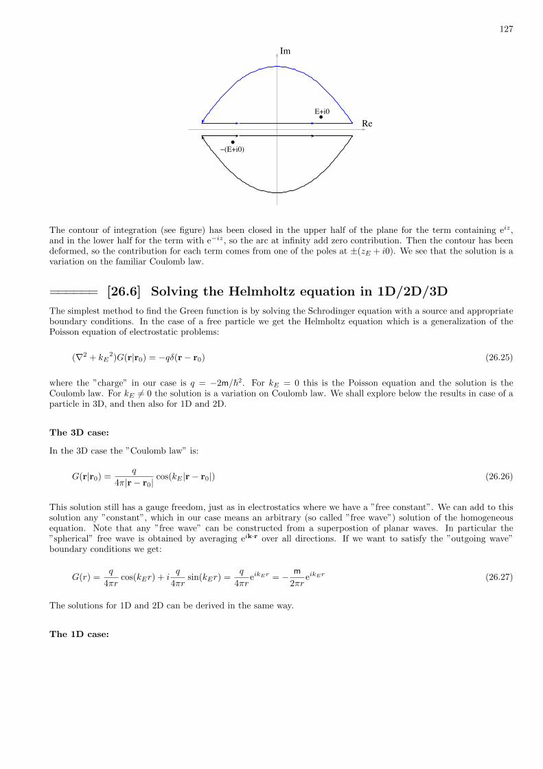
127

−(E+i0)

E+i0

Im

Re

The contour of integration (see figure) has been closed in the upper half of the plane for the term containing eiz,and in the lower half for the term with e−iz, so the arc at infinity add zero contribution. Then the contour has beendeformed, so the contribution for each term comes from one of the poles at ±(zE + i0). We see that the solution is avariation on the familiar Coulomb law.

====== [26.6] Solving the Helmholtz equation in 1D/2D/3D

The simplest method to find the Green function is by solving the Schrodinger equation with a source and appropriateboundary conditions. In the case of a free particle we get the Helmholtz equation which is a generalization of thePoisson equation of electrostatic problems:

(∇2 + kE2)G(r|r0) = −qδ(r− r0) (26.25)

where the ”charge” in our case is q = −2m/~2. For kE = 0 this is the Poisson equation and the solution is theCoulomb law. For kE 6= 0 the solution is a variation on Coulomb law. We shall explore below the results in case of aparticle in 3D, and then also for 1D and 2D.

The 3D case:

In the 3D case the ”Coulomb law” is:

G(r|r0) =q

4π|r− r0|cos(kE |r− r0|) (26.26)

This solution still has a gauge freedom, just as in electrostatics where we have a ”free constant”. We can add to thissolution any ”constant”, which in our case means an arbitrary (so called ”free wave”) solution of the homogeneousequation. Note that any ”free wave” can be constructed from a superpostion of planar waves. In particular the”spherical” free wave is obtained by averaging eik·r over all directions. If we want to satisfy the ”outgoing wave”boundary conditions we get:

G(r) =q

4πrcos(kEr) + i

q

4πrsin(kEr) =

q

4πreikEr = − m

2πreikEr (26.27)

The solutions for 1D and 2D can be derived in the same way.

The 1D case:

128

In the one dimensional case the equation that determines the Green function is

(∂2

∂x2+ k2

E

)G(x) = −qδ(x) (26.28)

where for simplicity we set x0 = 0. The delta function source requires a jump of the derivative G′(+0)−G′(−0) = −q.Using different phrasing: in order for the second derivative to be a delta function the first derivative must have a stepfunction. Thus, when kE = 0 we get the 1D Coulomb law G(x) = −(q/2)|x|, but for kE 6= 0 we have a variation onCoulomb law

G(x) = − q

2kEsin(kE |x|) (26.29)

(see figure). To this we can add any 1D free wave. In order to satisfy the ”outgoing waves” boundary conditions weadd cos(kx) = cos(k|x|) to this expression, hence we get the retarded Green’s function in 1D

G(x) = iq

2kEeikE |x| = −i m

kEeikE |x| (26.30)

−6 −4 −2 0 2 4 6−3

−2.5

−2

−1.5

−1

−0.5

0

0.5

x

G0(x

)

The 2D case:

In two dimensions for kE = 0 we use Gauss’ law to calculate the electrostatic field that goes like 1/r, and hence theelectrostatic potential is G(r) = −(1/(2π)) ln r. for kE 6= 0 we get the modulated result

G(r) = −q4

Y0(kEr) (26.31)

where Y0(x) is the Bessel function of the second kind

Y0′(x) = −Y1(x) (26.32)

Y0(x) ∼√

2

πxsin(x− π

4) , for large x

The second independent solution of the associated homogeneous equation is the Bessel function of the first kind J0(x).Adding this ”free wave” solution leads to a solution that satisfies the ”outgoing wave” boundary conditions. Hencewe get the retarded Green’s function in 2D

G(r) = iq

4H0(kEr) = −im

2H0(kEr) (26.33)

where H0(x) = J0(x) + iY0(x) is the Hankel function.

129

====== [26.7] Green function for a quasi 1D network

There is a very simple expression for the Green function of a particle that has energy E in a quasi 1D network (see”QM is practice” section):

G(x|x0) = −i 1

vE

∑p

Ap(E) eikELp (26.34)

where p labels trajectories that start at x0 and end at x. The length of a given trajectory is Lp, while Ap(E) isthe product of transmission and reflection amplitudes due to scattering at the nodes of the network. The proofof this formula is a straightforward generalization of the standard 1D case: The function Ψ(x) = G(x|x0) satisfiesthe Schrodinger equation for any x 6= x0, and in particular the matching conditions at the nodes are satisfied byconstruction. At x0 the function Ψ(x) has the same discontinuity as in the standard 1D case, because for the directtrajectory Lp = |x−x0| has a jump in its derivative. This discontinuity reflects having a source at x = x0 as required.

Delta scatterer.– Possibly the simplest quasi 1D networks, is a line with one node. We can describe the node as adelta function potential:

V (x) = uδ(x) = |0〉u〈0| (26.35)

In the last equality we point out that V (x) is essentially a projector |ψ〉〈ψ|. For this type of potential there is asimple inversion formula that we discuss below, that allows a direct evaluation of the resolvent. Optionally one cancalculate the reflection and the transmission coefficients for a delta function potential, and use the general formula ofthe previous paragraph, leading to

G(x|x0) = −i 1

vE

[eikE(x−x0) + reikE(|x|+|x0|)

](26.36)

where r is the reflection coefficient of a delta scatterer.

Inversion formula.– Given a state ψ we have the identity

1

1− |ψ〉λ〈ψ|= 1 +

1

1− λ|ψ〉λ〈ψ| (26.37)

This is proved by selecting an orthonormal basis that contains ψ as one of its states, such that the matrix in thedenominator is diag1−λ, 1, 1, 1, .... A generalization of this formula for any invertible A, and B = |ψ〉λ〈ψ| is

1

A−B=

1√A

[1− 1√

AB

1√A

]−11√A

=1

A+

(1

1− trace(A−1B)

)1

AB

1

A(26.38)

We can use this formula in order to find the resolvent in the case of a delta function:

G =1

(E −H0)− V= G0 +

(1

1− uG(E)

)G0V G0 ≡ G0 +G0TG0 (26.39)

where G(E) = G0(0|0), and T is like an effective interaction

T =

(1

1− uG(E)

)V =

u

1 + i(u/vE)δ(x) (26.40)

By inspection one can verify that this result is consistent with the result that we have cited at the beginning of thissection. We shall further discuss the significance of this expression and the details of the G(E) calculation in thelecture regarding the T matrix formalism.

130

====== [26.8] Semiclassical evaluation of the Green function

The semiclassical procedure, based on the Van-Vleck formula, provides a common approximation for all the specialcases that have been discussed above, and also allows further generalization. The Green function is the FT of thepropagator:

G(x|x0) ∼∫ ∞

0

eiAcl(x,x0)+iEtdt ∼ eiScl(x,x0) (26.41)

In order to derive the last expression one applies the stationary phase approximation for the evaluation of the dtintegral. The stationary point is determined by the equation Ecl = E where Ecl ≡ −dAcl/dt. The reduced action isdefined as

Scl(x, x0) = Acl + E =

∫ t

0

[Lcl + E]dt =

∫ x(t)

x(0)

pcl · dx (26.42)

It is implicit in this definition that the reduced action is evaluated for a classical trajectory that has energy E andconnects the points x(0) and x(t), and likewise the classical momentum pcl is evaluated along this trajectory.

====== [26.9] The boundary integral method

The Schrodinger equation Hψ = Eψ0 can be written as HEψ = 0 where

HE = −∇2 + UE(r) (26.43)

with UE(r) = U(r) − E. Green’s function solves the equation HEG(r|r0) = −qδ(r − r0) with q = −2m/~2. In thissection we follow the convention of electrostatics and set q = 1. From this point on we use the following (generalized)terminology:

Laplace equation [no source]: HEψ(r) = 0 (26.44)

Poisson equation: HEψ(r) = ρ(r) (26.45)

Definition of the Coulomb kernel: HEG(r|r0) = δ(r − r0) (26.46)

The solution of the Poisson equation is unique up to an arbitrary solution of the associated Laplace equation. If thecharge density ρ(r) is real, then the imaginary part of ψ(r) is a solution of the Laplace equation. Therefore withoutloss of generality we can assume that ψ(r) and G(r|r0) are real. From the definition of the Coulomb kernel it followsthat the solution of the Poisson equation is

Coulomb law: ψ(r) =

∫G(r|r′)ρ(r′)dr′ (26.47)

In particular we write the solution which is obtained if we have a charged closed boundary r = r(s). Assuming thatthe charge density on the boundary is σ(s) and that the dipole density (see discussion below) is d(s) we get:

ψ(r) =

∮ ([G(r|s)]σ(s) + [∂sG(r|s)]d(s)

)ds (26.48)

We use here the obvious notation G(r|s) = G(r|r(s)). The normal derivative ∂ = ~n · ∇ is taken with respect to thesource coordinate, where ~n is a unit vector that points outwards.

It should be obvious that the obtained ψ(r) solves the Laplace equation in the interior region, as well as in the exteriorregion, while across the boundary it satisfies the matching conditions

Gauss law: ∂ψ(s+)− ∂ψ(s−) = −σ(s) (26.49)

ψ(s+)− ψ(s−) = d(s) (26.50)

131

These matching conditions can be regarded as variations of Gauss law. They are obtained by integrating the Poissonequation over an infinitesimal range across the boundary. The charge density σ(s) implies a jump in the electric field−∂ψ(s). The dipole density d(s) is formally like a very thin parallel plates capacitor, and it implies a jump in thepotential ψ(s).

Let us ask the inverse question: Given a solution of Laplace equation in the interior region, can we find σ(s) and d(s)that generate it? The answer is yes. In fact, as implied from the discussion below, there are infinitely many possiblechoices. But in particular there is one unique choice that gives ψ(r) inside and zero outside. Namely, σ(s) = ∂ψ(s)and d(s) = −ψ(s), where ψ(s) = ψ(r(s)). Thus we get:

The bounday integral formula: ψ(r) =

∮ ([G(r|s)]∂ψ(s)− [∂sG(r|s)]ψ(s)

)ds (26.51)

The bounday integral formula allows to express the ψ(r) at an arbitrary point inside the domain using a boundaryintegral over ψ(s) and its normal derivative ∂ψ(s).

The standard derivation of the boundary integral formula is based on formal algebraic manipulations with Green’stheorem. We prefer below a simpler physics-oriented argumentation. If ψ(r) satisfies Laplace equation in the interior,and it is defined to be zero in the exterior, then it satisfies (trivially) the Laplace equation also in the exterior. Ontop it satisfies the Gauss matching conditions with σ(s) = ∂ψ(s−) and d(s) = −ψ(s−). Accordingly it is a solution ofthe Poisson equation with σ(s) and d(s) as sources. But for the same σ(s) and d(s) we can optionally obtain anothersolutions of the Poisson equation from the bounday integral formula. The two solutions can differ by a solution ofthe associated Laplace equation. If we supplement the problem with zero boundary conditions at infinity, the twosolutions have to coincide.

For the case where the wave function vanishes on the boundary ψ(s) = 0 the expression becomes very simple

ψ(r) =

∮G(r|s′)ϕ(s′)ds′ (26.52)

where ϕ(s) = ∂ψ(s), and in particular as we approach the boundary we should get:

∫G(s|s′)ϕ(s′)ds′ = 0 (26.53)

An obvious application of this formula leads to a powerful numerical method for finding eigenfunctions. This is theso called boundary integral method. Let us consider the problem of a particle in a billiard potential. Our Green’sfunction is (up to a constant)

G(s|s′) = Y0(kE |r(s)− r(s′)|) (26.54)

If we divide the boundary line into N segments then for any point on the boundary the equality∫G(s|s′)ϕ(s′)ds′ = 0

should hold, so:

∑j

Aijϕj = 0 with Aij = Y0(kE |r(si)− r(sj)|) (26.55)

Every time the determinant det(A) vanishes we get a non trivial solution to the equation, and hence we can constructan eigenfunction. So all we have to do is plot the determinant det(A) as a function of kE . The points where det(A)equals zero are the values of kE for which the energy E is an eigenvalue of the Hamiltonian H.

132

[27] Perturbation theory

====== [27.1] Perturbation theory for the resolvent

We first generalize the ”inversion formula” that has been introduced in the previous lecture. There it has been appliedto the exact calculation of the Green function for a delta function. Here we consider general matrices A and B, andpoint out the formal identity

1

(1−B)= (1−B)−1 =

∞∑n=0

Bn (27.1)

1

A−B= (A(1−A−1B))−1 = (1−A−1B)−1A−1 =

∑n

(A−1B)nA−1

=1

A+

1

AB

1

A+

1

AB

1

AB

1

A+ . . . (27.2)

Applying the above formal expansion for the calculation of the resolvent one obtains:

G(z) =1

z −H=

1

z − (H0 + V )=

1

(z −H0)− V(27.3)

= G0(z) +G0(z)V G0(z) +G0(z)V G0(z)V G0(z) + . . . (27.4)

Or, in matrix representation

G(x|x0) = G0(x|x0) +

∫G0(x|x2)dx2〈x2|V |x1〉dx1G0(x1|x0) + . . . (27.5)

Note that for the scalar potential V = u(x) we get

G(x|x0) = G0(x|x0) +

∫dx′G0(x|x′)u(x′)G0(x′|x0) + . . . (27.6)

====== [27.2] Perturbation Theory for the Propagator

For the Green function we get

G+(ω) = G+0 (ω) +G+

0 (ω)V G+0 (ω) +G+

0 (ω)V G+0 (ω)V G+

0 (ω) + . . . (27.7)

Recall that

G+(ω)→ FT → −iΘ(τ)U(τ) (27.8)

Then from the convolution theorem it follows that

(−i)[Θ(t)U(t)] = (−i)[ΘU0(t)] + (−i)2

∫dt′[Θ(t− t

′)U(t− t

′)] [V ] [Θ(t

′)U0(t

′)] + . . . (27.9)

which leads to

U(t) = U0(t) +

∞∑n=1

(−i)n∫

0<t1<t2<···<tn<tdtn . . . dt2dt1 U0(t− tn)V . . . U0(t2 − t1)V U0(t1) (27.10)

133

for t > 0 and zero otherwise. This can be illustrated diagrammatically using Feynman diagrams.

Let us see how we use this expression in order to get the transition probability formula. The first order expression forthe evolution operator is

U(t) = U0 − i∫dt′U0(t− t

′)V U0(t

′) (27.11)

Assume that the system is prepared in an eigenstate m of the unperturbed Hamiltonian, we get the amplitude to findit after time t in another eigenstate n is

〈n|U(t)|m〉 = e−iEntδnm − i∫dt′e−iEn(t−t

′)〈n|V |m〉e−iEmt

′

(27.12)

If n 6= m it follows that:

Pt(n|m) = |〈n|U(t)|m〉|2 =

∣∣∣∣∫ t

0

dt′Vnmei(En−Em)t′∣∣∣∣2 (27.13)

====== [27.3] Perturbation theory for the evolution

In this section we review the elementary approach to solve the evolution problem via an iterative scheme with theSchrodinger equation. Then we make the bridge to a more powerful procedure. Consider

|Ψ〉 =∑n

Ψn(t)|n〉 (27.14)

It follows that:

i∂Ψn

∂t= EnΨn +

∑n′

Vnn′Ψn′ (27.15)

We want to solve in the method which is called ”variation of parameters”, so we set:

Ψn(t) = cn(t)e−iEnt (27.16)

Hence:

dcndt

= −i∑n′

ei(En−En′ )tVnn′cn′(t) (27.17)

From the zero order solution cn(t) = δnm we get after one iteration:

cn(t) = δnm − i∫ t

0

dt′ei(En−Em)t′Vnm (27.18)

In order to make the connection with the formal approach of the previous and of the next section we write

cn = eiEntΨn =⟨n∣∣U−1

0 U(t)∣∣m⟩ ≡ 〈n|UI(t)|m〉 (27.19)

134

and note that

ei(En−Em)tVnm =⟨n∣∣U0(t)−1V U0(t)

∣∣m⟩ ≡ 〈n|VI(t)|m〉 (27.20)

Hence the above first order result can be written as

〈n|UI(t)|m〉 = δnm − i∫ t

0

〈n|VI(t′)|m〉 dt′ (27.21)

In the next sections we generalize this result to all orders.

====== [27.4] The Interaction Picture

First we would like to recall the definition of time ordered exponentiation

U(t, t0) = (1− idtNH(tN )) . . . (1− idt2H(t2))(1− idt1H(t1)) ≡ T e−i∫ tt0H(t′)dt′

(27.22)

Previously we have assumed that the Hamiltonian is not time dependent. But in general this is not the case, so wehave to keep the time order. The parenthesis in the above definition can be ”opened” and then we can assemble theterms of order of dt. Then we get the expansion

U(t, t0) = 1− i(dtNH(tN )) · · · − i(dt1H(t1)) + (−i)2(dtNH(tN ))(dtN−1H(tN−1)) + . . . (27.23)

= 1− i∫t0<t′<t

H(t′)dt′ + (−i)2

∫t0<t′<t′′<t

H(t′′)H(t′)dt′′dt′ + . . .

=

∞∑n=0

(−i)n∫t0<t1<t2···<tn<t

dtn . . . dt1H(tn) . . .H(t1)

Note that if H(t′) = H is not time dependent then we simply get the usual Taylor expansion of the exponentialfunction where the 1/n! prefactors would come from the time ordering limitation.

The above expansion is not very useful because the sum is likely to be divergent. What we would like to consider isthe case

H = H0 + V (27.24)

where V is a small perturbation. The perturbation V can be either time dependent or time independent. It isconvenient to regard the evolution as a sequence of ”free” evolution during [t0, 0], an interaction at t = 0, and a later”free” evolution during [0, t]. Consequently we define a unitary operator UI such that

U(t, t0) = U0(t, t0)UI U0(0, t0) (27.25)

Accordingly UI = 1 if V = 0. Otherwise UI gives the effect of the interaction as if it happened at the referencetime t = 0. For simplicity we adopt from now on the convention t0 = 0, and use the notation U(t) instead of U(t, t0).Thus

UI ≡ U0(t)−1 U(t) (27.26)

We also define the following notation

VI(t) = U0(t)−1 V U0(t) (27.27)

135

By definition of H as the generator of the evolution:

d

dtU(t) = −i(H0 + V ) U(t) (27.28)

Consequently:

d

dtUI = −iVI(t) UI (27.29)

The solution is by time ordered exponentiation

UI = T exp

(−i∫ t

0

VI(t′)dt′

)=

∞∑n=0

(−i)n∫

0<t1<t2···<tn<tdtn . . . dt1 VI(tn) . . . VI(t1) (27.30)

Which can be written formally as

UI =

∞∑n=0

(−i)n

N !

∫ t

0

dtn . . . dt1 T VI(tn) . . . VI(t1) (27.31)

Optionally we can switch back to the Schrodinger picture:

U(t) =

∞∑n=0

(−i)n∫

0<t1<t2<···<tn<tdtn . . . dt2dt1 U0(t− tn)V . . . U0(t2 − t1)V U0(t1) (27.32)

The latter expression is more general than the one which we had obtained via FT of the resolvent expansion, becausehere V is allowed to be time dependent.

====== [27.5] The Kubo formula

Consider the special case of having a time dependent perturbation V = −f(t)B. The first order expression for theevolution operator in the interaction picture is

UI(t) = 1 + i

∫ t

0

AI(t′)f(t′)dt′ (27.33)

where AI(t) is A in the interaction picture. If our interest is in the evolution of an expectation value of another

observable A, then we have the identity

〈A〉t = 〈ψ(t)|A|ψ(t)〉 = 〈ψ|AH(t)|ψ〉 = 〈ψ|UI(t)−1AI(t)UI(t)|ψ〉 (27.34)

To leading order we find

〈A〉t = 〈AI(t)〉 +

∫ t

0

α(t, t′)f(t′)dt′ (27.35)

where the linear response kernel is given by the Kubo formula:

α(t, t′) = i〈[AI(t), BI(t′)]〉 (27.36)

136

In the above formulas expectation values without subscript are taken with the state ψ. It should be clear that theKubo formula is merely the interaction picture version of the “rate of change” formula: The rate of change of theexpectation value of A is determined by the expectation value of the commutator [H, A], hence in the interactionpicture it is determined by the expectation value of [VI , AI ].

====== [27.6] The S operator

The formula that we have found for the evolution operator in the interaction picture can be re-written for an evolutionthat starts at t = −∞ (instead of t = 0) and ends at t =∞. For such scenario we use the notation S instead of UIand write:

S =

∞∑n=0

(−i)n

N !

∫ +∞

−∞dtn . . . dt1 T VI(tn) . . . VI(t1) (27.37)

It is convenient to regard t = −∞ and t =∞ as two well defined points in the far past and in the far future respectively.The limit t→ −∞ and t→∞ is ill defined unless S is sandwiched between states in the same energy shell, as in thecontext of time independent scattering.

The S operator formulation is useful for the purpose of obtaining an expression for the temporal cross-correlationof (say) two observables A and B. The type of system that we have in mind is (say) a Fermi sea of electrons. Theinterest is in the the ground state ψ of the system which we can regard as the “vacuum state”. The object that wewant to calculate, written in the Heisenberg / Schrodinger / Interaction pictures is

CBA(t2, t1) = 〈ψ|BH(t2)AH(t1)|ψ〉 (27.38)

= 〈ψ|U(t2)−1B U(t2, t1)AU(t1) |ψ〉 (27.39)

= 〈ψ|UI(t2)−1BI(t2)UI(t2, t1)AI(t1)UI(t1) |ψ〉 (27.40)

where it is implicitly assumed that t2 > t1 > 0, and we use the notation UI(t2, t1) = UI(t2)UI(t1)−1, which is the

evolution operator in the interaction picture referenced to the time t1 rather than to t=0. Note that S = UI(∞,−∞).Assuming that ψ is obtained from the non-interacting ground state φ via an adiabatic switching of the perturbationduring the time −∞ < t < 0 we can rewrite this expression as follows:

CBA(t2, t1) = 〈φ|UI(∞,−∞)−1 UI(∞, t2)BI(t2)UI(t2, t1)AI(t1)UI(t1,−∞) |φ〉 (27.41)

= 〈φ| S† T S BI(t2)AI(t1) |φ〉 (27.42)

In the last line it is implicit that one should first substitute the expansion for S, and then (prior to integration)perform the time ordering of each term. The Gell-Mann-Low theorem rewrites the above expression as follows:

〈ψ|T BH(t2)AH(t1)|ψ〉 =〈φ|T SBI(t2)AI(t1)|φ〉

〈φ|S|φ〉= 〈φ|T SBI(t2)AI(t1)|φ〉connected (27.43)

The first equality follows from the observation that due to the assumed adiabaticity the operation of S on φ is merelya multiplication by a phase factor. The second equality is explained using a diagrammatic language. Each term in theperturbative expansion is illustrated by a Feynman diagram. It is argued that the implicit unrestricted summationof the diagrams in the numerator equals to the restricted sum over all the connected diagrams, multiplied by theunrestricted summation of vacuum-to-vacuum diagrams (as in the numerator). The actual diagrammatic calculationis carried out by applying Wick’s theorem. The details of the diagrammatic formalism are beyond the scope of ourpresentation.

137

[28] Complex poles from perturbation theory

====== [28.1] Models of interest

In this section we solve the particle decay problem using perturbation theory for the resolvent. We are going to showthat for this Hamiltonian the analytical continuation of the resolvent has a pole in the lower part of the complexz-plane. The imaginary part (”decay rate”) of the pole that we find is the same as we found by either the Fermigolden rule or by the exact solution of the Schrodinger equation.

We imagine that we have an ”unperturbed problem” with one energy level |0〉 of energy E0 and a continuum of levels|k〉 with energies Ek. A model of this kind may be used for describing tunneling from a metastable state. Anotherapplication is the decay of an excited atomic state due to emission of photons. In the latter case the initial state wouldbe the excited atomic state without photons, while the continuum are states such that the atom is in its ground stateand there is a photon. Schematically we have

H = H0 + V (28.1)

where we assume

〈k|V |0〉 = σk (coupling to the continuum) (28.2)

〈k′|V |k〉 = 0 (no transitions within the continuum)

Due to gauge freedom we can assume that the coupling coefficients are real numbers without loss of generality. TheHamiltonian matrix can be illustrated as follows:

H =

E0 σ1 σ2 σ3 . . . σk .σ1 E1 0 0 . . . 0 .σ2 0 E2 0 . . . 0 .σ3 0 0 E3 . . . 0 .. . . . . . . 0 .. . . . . . . 0 .. . . . . . . 0 .σk 0 0 0 0 0 0 Ek .. . . . . . . . .

(28.3)

We later assume that the system under study is prepared in state |0〉 at an initial time (t = 0), and we want to obtainthe probability amplitude to stay in the initial state at a later times.

It is important to notice the following (a) we take one state and neglect other states in the well. (b) we assume that Vallows transitions from this particular state in the well (zero state |0〉) into the |k〉 states in the continuum, while we donot have transitions in the continuum itself. These assumptions allow us to make exact calculation using perturbationtheory to infinite order. The advantage of the perturbation theory formalism is that it allows the treatment of morecomplicated problems for which exact solutions cannot be found.

====== [28.2] Heuristic approach

The Hamiltonian of the previous section is of the form

H = H0 + V =

(HP

0 0

0 HQ0

)+

(0 V PQ

V QP 0

)(28.4)

and the wavefunction can be written as

Ψ =

(ψχ

)(28.5)

138

In the decay problem of the previous section HP0 is a 1× 1 matrix, and HQ

0 is an ∞×∞ matrix. The perturbationallows transitions between P and Q states. In the literature it is customary to define projectors P and Q on therespective sub-spaces.

P +Q = 1 (28.6)

Our interest is focused only in the ψ piece of the wavefunction, which describes the state of the particle in the P space.On the other hand we assume that H has a continuous spectrum, and therefore any E above the ground state definesa stationary state via the equation

(HP

0 V PQ

V QP HQ0

)(ψχ

)= E

(ψχ

)(28.7)

From the second raw of the above equation it follows that χ = GQV QPψ, where GQ0 = 1/(E −HQ0 ). Consequently

the reduced equation for ψ is obtained from the first raw of the matrix equation

[HP

0 + V PQGQV QP]ψ = Eψ (28.8)

The second term in the square brackets Σ(E) = V PQGQ0 VQP is the so called ”self energy”. Using the vague prescrip-

tion E 7→ E + i0 we can split it into an effective potential due to so called ”polarization cloud” (also known as Lambshift) and an imaginary part due to FGR decay:

HP = HP0 + ∆− iΓ/2 (28.9)

∆ij =∑k∈Q

VikVkjE − Ek

(28.10)

Γij = 2π∑k∈Q

VikVkjδ(E − Ek) (28.11)

We argue that HP generates the time evolution of ψ within P space. This effective Hamiltonian is non-hermitianbecause probability can escape to the Q space. It can be diagonalized so as to get the decay modes of the system.Each mode is characterized by its complex energy Er − i(Γr/2). Note that the effective Hamiltonian is non-hermitianand therefore the eigen-modes are in general non-orthogonal [see discussion of generalized spectral decomposition inthe Fundementals I section].

The advantage of the above treatment is its technical simplicity. However, the mathematical significance of theE 7→ E + i0 prescription is vague. We therefore turn to a more formal derivation of the same result, which illuminateshow the non-hermiticity emerges once the Q continuum is eliminated.

====== [28.3] The P +Q formalism

We want to calculate the resolvent. But we are interested only in the single matrix element (0, 0) because we want toknow the probability to stay in the |0〉 state:

survival probability =∣∣∣FT

[〈0|G(ω)|0〉

]∣∣∣2 (28.12)

Here G(ω) is the retarded Green function. More generally we may have several states in the well. In such a caseinstead of P = |0〉〈0| we have

P =∑

n∈well

|n〉〈n| (28.13)

139

If we prepare the particle in an arbitrary state Ψ inside the well, then the probability to survive in the same state is

survival probability =∣∣∣FT

[〈Ψ|G(ω)|Ψ〉

]∣∣∣2 =∣∣∣FT

[〈Ψ|GP (ω)|Ψ〉

]∣∣∣2 (28.14)

Namely, we are interested only in one block of the resolvent which we call

GP (z) = PG(z)P (28.15)

Using the usual expansion we can write

GP = PGP = P1

z − (H0 + V )P = P (G0 +G0V G0 + . . . )P (28.16)

= PG0P + PG0(P +Q)V (P +Q)G0P + PG0(P +Q)V (P +Q)G0(P +Q)V (P +Q)G0P + . . .

= GP0 +GP0 ΣPGP0 +GP0 ΣPGP0 ΣPGP0 + . . .

=1

z − (HP0 + ΣP )

where the ”self energy” term

ΣP = V PQGQ0 VQP (28.17)

represents the possibility of making a round trip out of the well. Note that only even order terms contribute to thisperturbative expansion because we made the simplifying assumption that the perturbation does not have ”diagonalblocks”. In our problem ΣP is a 1× 1 matrix that we can calculate as follows:

ΣP =∑k

〈0|V |k〉〈k|G0|k〉〈k|V |0〉 =∑k

|Vk|2

E − Ek + i0(28.18)

=∑k

|Vk|2

E − Ek− iπ

∑k

|Vk|2δ(E − Ek) ≡ ∆0 − i(Γ0/2)

In the last step we have implicitly assumed that our interest is in the retarded Green function. We have identified asbefore the Fermi golden rule rate

Γ0 = 2π∑k

|Vk|2δ(E − Ek) ≡ 2π%(E) |V |2 (28.19)

Thus, the resolvent is the 1× 1 matrix.

GP (z) =1

z − (HP0 + ΣP )

=1

z − (ε0 + ∆0) + i(Γ0/2)(28.20)

We see that due to the truncation of the Q states we get a complex Hamiltonian, and hence the resolvent has a polein the lower plane. The Fourier transform of this expression is the survival amplitude. After squaring it gives a simpleexponential decay e−Γt.

140

Scattering Theory

[29] The plane wave basisThere are several different conventions for the normalization of plane waves:• Box normalized plane waves |n〉• Density normalized plane waves |k〉• Energy shell normalized plane waves |E,Ω〉

We are going to be very strict in our notations, else errors are likely. We clarify the three conventions first in the 1Dcase, and later in the 3D case, and then to remark on energy shell bases in general.

====== [29.1] Plane waves in 1D

The most intuitive basis set originates from quantization in a box with periodic boundary conditions (a torus):

|n〉 −→ 1√L

eiknx (29.1)

where

kn =2π

Ln (29.2)

Orthonormality:

〈n|m〉 = δnm (29.3)

Completeness:

∑n

|n〉〈n| = 1 (29.4)

The second convention is to have the density normalized to unity:

|k〉 −→ eikx (29.5)

Orthonormality:

〈k|k′〉 = 2πδ(k − k′) (29.6)

Completeness:∫|k〉dk

2π〈k| = 1 (29.7)

Yet there is a third convention which assumes that the states are labeled by their energy, and by another index thatindicate the direction.

|E,Ω〉 =1√vE|kΩ〉 −→

1√vE

eikΩx (29.8)

141

where 0 < E <∞ and Ω is the direction of propagation with nΩ = ±1, hence

kΩ = nΩkE = ±√

2mE (29.9)

Orthonormality:

〈E,Ω|E′,Ω′〉 = 2πδ(E − E′)δΩΩ′ (29.10)

Completeness:∫dE

2π

∑Ω

|E,Ω〉〈E,Ω| = 1 (29.11)

In order to prove the orthonormality we note that dE = vEdk and therefore

δ(E − E′) =1

vEδ(k − k′) (29.12)

The energy shell normalization of plane waves in 1D is very convenient also for another reason. We see that theprobability flux of the plane waves is normalized to unity. We note that this does not hold in more than 1D. Still alsoin more than 1D, the S matrix formalism reduces the scattering problem to 1D channels, and therefore this propertyis very important in general.

====== [29.2] Plane waves in 3D

The generalization of the box normalization convention to the 3D case is immediate. The same applied to the densitynormalized plane waves:

|~k〉 −→ ei~k~x (29.13)

Orthonormality:

〈~k|~k′〉 = (2π)3δ3(~k − ~k′) (29.14)

Completeness:

∫|~k〉 d

3k

(2π)3〈~k| = 1 (29.15)

The generalization of the energy shell normalization convention is less trivial:

|E,Ω〉 =1

2π

kE√vE|~kΩ〉 −→

1

2π

kE√vE

ei~kΩ·~x (29.16)

where we define the direction by Ω = (θ, ϕ), with an associated unit vector ~nΩ and a wavenumber

~kΩ = kE~nΩ (29.17)

Orthonormality:

〈E,Ω|E′,Ω′〉 = 2πδ(E − E′)δ2(Ω− Ω′) (29.18)

142

Completeness:

∫dE

2π

∫|E,Ω〉dΩ〈E,Ω| = 1 (29.19)

To prove the identities above we note that

d3k = k2dkdΩ = k2E

dE

vEdΩ = k2

E

dE

vEdϕd cos θ (29.20)

and

δ3(~k − ~k′) =vEk2E

δ(E − E′)δ2(Ω− Ω′) =vEk2E

δ(E − E′)δ(ϕ− ϕ′)δ(cos θ − cos θ′) (29.21)

In general we have to remember that any change of the ”measure” is associated with a compensating change in thenormalization of the delta functions.

====== [29.3] Optional energy shell bases

Instead of the standard energy shell basis |E,Ω〉 one can use some other basis |E, a〉, where a is a quantum numberthat labels the different basis states. In particular in 3D problem it is convenient to use the |E, `m〉 basis:

〈E′,Ω|E, `m〉 = 2πδ(E′ − E) Y `m(Ω) (29.22)

Note that in position representation we have

〈r,Ω|E, `m〉 = 2kE√vE

j`(kEr) Y`m(Ω) (29.23)

This wavefunction is properly normalized as an energy-shell basis state. The asymptotic behaviour of the sphericalBessel function is j`(kr) ∼ sin(kr − phase)/(kr), and accordingly, as in the 1D case, this wavefunction is also ”fluxnormalized”: the flux of both the ingoing and the outgoing wave components is unity.

143

[30] Scattering in the T -matrix formalism

====== [30.1] The Scattering States

Our purpose is to solve the Schrodinger’s equation for a given energy E.

(H0 + V )Ψ = EΨ (30.1)

If we rearrange the terms, we get:

(E −H0 − V )Ψ = 0 (30.2)

In fact we want to find scattering solutions. These are determined uniquely if we define what is the ”incident wave”and require outgoing boundary conditions for the scattered component. Thus we write Ψ as a superposition of a freewave and a scattered wave,

Ψ = φ+ Ψscatt (30.3)

The scattered wave Ψscatt is required to satisfy outgoing boundary conditions. The free wave φ is any solution of:

H0φ = Eφ (30.4)

Substituting, we obtain:

(E −H0 − V )Ψscatt = V φ (30.5)

with the solution Ψscatt = G+V φ, leading to:

Ψ = (1 +G+V )φ (30.6)

====== [30.2] The Lippman Schwinger equation

The explicit solution for Ψ that was found in the previous section is in typically useless, because it is difficult to get G.A more powerful approach is to write an integral equation for Ψ. For this purpose we re-arrange the differentialequation as

(E −H0)Ψ = VΨ (30.7)

Using exactly the same procedure as in the previous section we get

Ψ = φ+G+0 VΨ (30.8)

This Lippman Schwinger equation can be solved for Ψ using standard techniques (see example in the next section).More generally closed analytical solutions cannot be obtained. Still if V is small we can try to find a solution iteratively,starting with the free wave as a zero order solution. This leads to a perturbative expansion for Ψ which we are goingto derive in a later section using a simpler approach.

144

====== [30.3] Example: scattering by a regularized delta function

Let us demonstrate the procedure of solving Lippman Schwinger equation for scattering on a delta potential uδ(x) inone dimension. The relation Ψ = φ+G+

0 VΨ is written as

Ψ(x) = eikx − i uvE

Ψ(0)eik|x| (30.9)

Setting x = 0 we obtain a closed equation for the unknown wave amplitude Ψ(0), whose solution leads to

Ψ(x) = eikx + reik|x|, r =−i(u/vE)

1 + i(u/vE)(30.10)

where r is identified as the reflection coefficient, while the transmission coefficient is t = 1 + r.

It is instructive to consider the more general case of scattering by a regularized delta function in any dimension, andwith any dispersion relation. This generalization is also known as s-scattering. In particular it illuminates how adivergent series for the T matrix (see next section) can give a finite result, and why in the absence of regularizationa delta function does not scatter in more than one dimension. By a regularized delta function we mean a potentialV (x) whose non-zero matrix elements are

Vk,k′ = u, for |k|, |k′| < Λ (30.11)

where Λ is a large momentum cutoff. The Lippman Schwinger equation reads

Ψ(x) = φ(x) +∑k,k′

〈x|G+0 |k〉Vk,k′〈k′|Ψ〉 (30.12)

The sum over k and k′ factorizes, hence the second term in the right hand side can be approximated as uG+0 (x|0)Ψ(0).

Setting x = 0 we obtain a closed equation for the unknown wave amplitude Ψ(0), whose solution leads to

Ψ(x) = φ(x) +G+0 (x|0) ueffφ(0), ueff =

u

1− uG(E)(30.13)

where G(E) = G+0 (0|0). The above expression for Ψ(x) can be written as Ψ = (1 +G+

0 T )φ where

T = ueff δ(x) (30.14)

In the next section we further discuss the significance of T , which can be regarded as a renormalized version of thepotential V = uδ(x).

We now turn to discuss the practical calculation of G(E). From the definition it follows that

G(E) = G+0 (0|0) =

∑k

1

E − Ek + i0(30.15)

The k summation should be treated with the appropriate integration measure. It equals −i/vE for a non-regularizedDirac delta function in one dimension. In higher dimensions G(E) has a real part that diverges, which implies thatthe scattering goes to zero. The regularization makes G(E) finite. In three dimensions we get G(E) = −(m/π2)ΛEwhere

ΛE = −2π2

∫ Λ

0

d3k

(2π)3

1

k2E − k2 + i0

= Λ− 1

2kE log

(Λ + kEΛ− kE

)+ i

π

2kE (30.16)

145

Another interesting case to consider is having (say) a constant density of states with a threshold energy. The divergenceof G(E) near a threshold is logarithmic. It is quite amusing that the second order as well as all the higher terms inperturbation theory are divergent, while their sum goes to zero...

====== [30.4] Perturbation Theory for the Scattering State

Going back to the formal solution for Ψ we can substitute there the perturbative expansion of G

G = G0 +G0V G0 +G0V G0V G0 + . . . (30.17)

leading to

Ψ = (1 +G+V )φ = φ+G0V φ+G0V G0V φ+ . . . (30.18)

As an example consider the typical case of scattering by a potential V (x). In this case the above expansion to leadingorder in space representation is:

Ψ(x) = φ(x) +

∫G0(x, x′)V (x′)φ(x′) dx′ (30.19)

====== [30.5] The T matrix

It is customary to define the T matrix as follows

T = V + V G0V + V G0V G0V + . . . = V + V GV (30.20)

The T matrix can be regarded as a ”corrected” version of the potential V , so as to make the following first orderlook-alike expression exact:

G = G0 +G0TG0 (30.21)

Or the equivalent expression for the wavefunction:

Ψ = φ+G+0 Tφ (30.22)

Later it is convenient to take matrix elements in the unperturbed basis of free waves:

Vαβ =⟨φα |V |φβ

⟩(30.23)

Tαβ(E) =⟨φα |T (E)|φβ

⟩In principle we can take the matrix elements between any states. But in practice our interest is in states that havethe same energy, namely Eα = Eβ = E. Therefore it is convenient to use two indexes (E, a), where the index adistinguishes different free waves that have the same energy. In particular a may stand for the ”direction” (Ω) of theplane wave. Thus in practice we are interested only in matrix elements ”on the energy shell”:

Tab(E) =⟨φE,a |T (E)|φE,b

⟩(30.24)

One should be very careful to handle correctly the different measures that are associated with different type of indexes.In particular note that in 3D:

TΩ,Ω0 =1

vE

(kE2π

)2

TkΩ,kΩ0(30.25)

146

====== [30.6] Scattering states in 1D problems

In this section we look for a scattering solution that originates from the free wave |k0〉. Using the result of a previoussection we write Ψ = φk0 +G+

0 Tφk0 with

φk0(r) = eik0x [density normalized] (30.26)

In Dirac notations:

|Ψ〉 = |φk0〉+G+0 T |φk0〉 (30.27)

In space representation:

〈x|Ψ〉 = 〈x|φk0〉+ 〈x|G+0 T |φk0〉 (30.28)

or in ”old style” notation:

Ψ(x) = φk0(x) +

∫G+

0 (x|x0)dx0〈x0|T |k0〉 (30.29)

In 1D problems the Green function is

G+0 (x|x0) = 〈x|G+

0 |x0〉 = − i

vEeikE |x−x0| (30.30)

Thus we get:

ψ(x) = ei~k0x − i

vE

∫eikE |x−x0|dx0〈x0|T |k0〉 (30.31)

By observation of the left asymptotic region we deduce that the reflection coefficient is

r = − i

vE〈−k0|T |k0〉 (30.32)

By observation of the right asymptotic region we deduce that the transmission coefficient is

t = 1− i

vE〈k0|T |k0〉 = 1 + r (30.33)

We note that conservation of probability implies |r|2 + |t|2 = 1. With the substitution of the above relation (t = 1 + r)it follows that

|r|2 = −Re[r] (30.34)

This is a special example for an ”optical theorem” that we shall discuss later on: it relates the total cross section (here2|r|2) to the ”forward” scattering amplitude. In order to understand this terminology note that r is the amplitude ofthe scattered wave both in the ”backward” and ”forward” directions while t is the sum of the forward scattering withthe incident wave. The above relation implies

scattering phase shift = arccos(r) (30.35)

147

====== [30.7] Scattering states in 3D problems

The derivation is the 3D case follows the same procedure as in the 1D case. The incident wave is

φk0(r) = ei~k0·~r [density normalized] (30.36)

and the implied scattering state is

Ψ(r) = φk0(r) +

∫G+

0 (r|r0)dr0〈r0|T |k0〉 (30.37)

where

G+0 (r|r0) = 〈r|G+

0 |r0〉 = − m

2π

eikE |r−r0|

|r − r0|(30.38)

Thus we get

Ψ(r) = φk0(r)− m

2π

∫eikE |r−r0|

|r − r0|〈r0|T |k0〉 dr0 (30.39)

So far everything is exact. Now we want to get a simpler expression for the asymptotic form of the wavefunction.Note that from the experimental point of view only the ”far field” region (far away from the target) is of interest.The major observation is that the dr0 integration is effectively bounded to the scattering region |r| < r0 where thematrix elements of V and hence of T are non-zero. Therefore for |r| |r0| we can use the approximation

|~r − ~r0| =√

(~r − ~r0)2 =√|r|2 − 2~r · ~r0 +O(|r0|2) ≈ |r|

[1− ~nΩ ·

~r0

|r|

]= |r| − ~nΩ · ~r0 (30.40)

Here and below we use the following notations:

~r ≡ |r|~nΩ (30.41)

Ω = (θ, ϕ) = spherical coordinates

~nΩ = (sin θ cosφ, sin θ sinφ, cos θ)

~kΩ = kE~nΩ

φ

θ

k 0

k Ω

z

x

y

rr0

148

With the approximation above we get:

Ψ(r) ≈ ei~k0·~r − m

2π

eikE |r|

r

∫e−i

~kΩ·~r0〈r0|T |k0〉 dr0 ≡ ei~k0·~r + f(Ω)

eikE |r|

|r|(30.42)

where

f(Ω) = − m

2π〈~kΩ|T (E)|~k0〉 (30.43)

It follows that the differential cross section is

dσ

dΩ= |f(Ω)|2 =

( m

2π~

)2∣∣∣∣1~TkΩ,k0

∣∣∣∣2 (30.44)

This formula assumes density normalized plane waves. It relates the scattering which is described by f(Ω) to the Tmatrix. It can be regarded as a special case of a more general relation between the S matrix and the T matrix, asdiscussed in later sections (and see in particular the discussion of the ”optical theorem” below).

====== [30.8] Born approximation and beyond

For potential scattering the first order approximation T ≈ V leads to the Born approximation:

f(Ω) = − m

2π〈~kΩ|T (E)|~k0〉 ≈ −

m

2πV (q) (30.45)

where ~q = ~kΩ − ~k0 and V (~q) is the Fourier transform of V (~r). The corresponding formula for the cross section isconsistent with the Fermi golden rule.

It is customary in high energy physics to take into account higher orders. The various terms in the expansion areillustrated using Feynman diagrams. However, there are circumstance where we can gain better insight by consideringthe analytical properties of the Green function. In particular we can ask what happens if G has a pole at some complexenergy z = Er − i(Γr/2). Assuming that the scattering is dominated by that resonance we get that the cross sectionhas a Lorentzian line shape. More generally, If there is an interference between the resonance and the non-resonantterms then we get a Fano line shape. We shall discuss further resonances later on within the framework of the Smatrix formalism.

====== [30.9] The Optical Theorem

From the energy-shell matrix elements of the T operator we can form an object that later we identify as the S matrix:

Sab = δab − i〈E, a|T |E, b〉 (30.46)

Using a more sloppy notation the equation above can be written as S = 1 − iT . We should remember that S is notan operator, and that Sab are not the matrix elements of an operator. In contrast to that Tab are the on-shell matrixelements of an operator. This relation assumes that the energy shell basis states are properly normalized.

The S matrix, as we define it later, is unitary. So we have S†S = 1, and therefore we conclude that the T matrixshould satisfy the following equality:

(T † − T ) = iT †T (30.47)

In particular we can write:

〈a0|T − T †|a0〉 = −i∑a

〈a0|T |a〉〈a|T †|a0〉 (30.48)

149

and we get:

∑a

|Taa0|2 = −2Im[Ta0a0

] (30.49)

This so called ”optical theorem” establishes a connection between the ”cross section” and the forward scatteringamplitude Ta0a0

. It should be clear that if this relation holds in one particular energy-shell basis, then it holds alsoin any other (properly normalized) energy shell basis. In 3D scattering problems we can write one of the followingexpressions:

∑`,m

|〈φE,`,m|T |φE,`0,m0〉|2 = −2Im[〈φE,l0,m0 |T |φE,l0,m0〉] (30.50)

∑Ω

|〈φE,Ω|T |φE,Ω0〉|2 = −2Im[〈φE,Ω0 |T |φE,Ω0〉]

Using the relations

|E,Ω〉 =1√vE

kE2π|kΩ〉 (30.51)

f(Ω) = − m

2π〈~kΩ|T (E)|~k0〉

we get

∫|〈~kΩ|T |~k0〉|2dΩ = −2vE

(2π

kE

)2

Im[〈~k0|T |~k0〉] (30.52)

Or the more familiar version:

σtotal =

∫|f(Ω)|2dΩ =

4π

kEIm[f(0)] (30.53)

150

[31] Scattering in the S-matrix formalism

====== [31.1] Channel Representation

Before we define the S matrix, Let us review some of the underlying assumptions of the S matrix formalism. Define

ρ(x) = |Ψ(x)|2 (31.1)

The continuity equation is

∂ρ

∂t= −∇ · J (31.2)

We are working with a time-independent Hamiltonian and looking for stationary solutions, hence:

∇ · J = 0 (31.3)

The standard basis for representation is |x〉. We assume that the wave function is separable outside of the scatteringregion. Accordingly we arrange the basis as follows:

|x ∈ inside〉 = the particle is located inside the scattering region (31.4)

|a, r〉 = the particle is located along one of the outside channels

and write the quantum state in this representation as

|Ψ〉 =∑

x∈inside

ϕ(x) |x〉 +∑a,r

Ra(r) |a, r〉 (31.5)

The simplest example for a system that has (naturally) this type of structure is a set of 1D wires connected togetherto some ”dot”. In such geometry the index a distinguishes the different wires. Another, less trivial example, is a leadconnected to a ”dot”. Assuming for simplicity 2D geometry, the wavefunction in the lead can be expanded as

Ψ(x) = Ψ(r, s) =∑a

Ra(r)χa(s) (31.6)

where the channel functions (waveguide modes) are:

χa(s) =

√2

`sin((π

`a)s)

with a = 1, 2, 3 . . . and 0 < s < ` (31.7)

In short, we can say that the wavefunction outside of the scattering region is represented by a set of radial functions:

Ψ(x) 7→ Ra(r) where a = 1, 2, 3 . . . and 0 < r <∞ (31.8)

The following figures illustrate several examples for scattering problems (from left to right): three connected wires,dot-waveguide system, scattering in spherical geometry, and inelastic scattering. The last two systems will be discussedbelow and in the exercises.

151

====== [31.2] The Definition of the S Matrix

Our Hamiltonian is time-independent, so the energy E is a good quantum number, and therefore the HamiltonianH is block diagonal if we take E as one index of the representation. For a given energy E the Hamiltonian has aninfinite number of eigenstates which form the so called ”energy shell”. For example in 3D for a given energy E we

have all the plane waves with momentum |~k| = kE , and all the possible superpositions of these waves. Once we areon the energy shell, it is clear that the radial functions should be of the form

Ra(r) = AaRE,a,−(r)−BaRE,a,+(r) (31.9)

For example, in case of a waveguide

RE,a,±(r) =1√va

e±ikar [flux normalized] (31.10)

where the radial momentum in channel a corresponds to the assumed energy E,

ka =

√2m

(E − 1

2m

(π`a)2)

(31.11)

and the velocity va = ka/m in channel a is determined by the dispersion relation. Thus on the energy shell thewavefunctions can be represented by a set of ingoing and outgoing amplitudes:

Ψ(x) 7−→ (Aa, Ba) with a = 1, 2, 3 . . . (31.12)

But we should remember that not all sets of amplitudes define a stationary energy state. In order to have a validenergy eigenstate we have to match the ingoing and outgoing amplitudes on the boundary of the scattering region.The matching condition is summarized by the S matrix.

Bb =∑a

SbaAa (31.13)

By convention the basis radial functions are ”flux normalized”. Consequently the current in channel a is Ia =|Ba|2 − |Aa|2 and from the continuity equation it follows that

∑a

|Ba|2 =∑a

|Aa|2 (31.14)

From here follows that the S matrix is unitary. The unitarity of the S matrix sometimes implies surprising conse-quences. For example: in 1D the transmission from-left-to-right must be equal to the transmission from-right-to-left.More generally: if we have a system with two different leads 1 and 2 then

∑a∈1,b∈2 |Sba|2 =

∑a∈2,b∈1 |Sba|2. The

latter observation is essential for the theory of the two-terminal Landauer conductance.

152

In order to practice the definition of the S matrix consider a system with a single 2D lead. Let us assume that thelead has 3 open channels. That means that ka is a real number for a = 1, 2, 3, and becomes imaginary for a > 3. Thea > 3 channels are called ”closed channels” or ”evanescent modes”. They should not be included in the S matrixbecause if we go far enough they contribute nothing to the wavefunction (their contribution decays exponentially).Thus we have a system with 3 open channels, and we can write

R1(r) =1√v1

(A1e−ik1r −B1e+k1r) (31.15)

R2(r) =1√v2

(A2e−ik2r −B2e+k2r)

R3(r) =1√v3

(A3e−ik3r −B3e+k3r)

and B1

B2

B3

= S

A1

A2

A3

(31.16)

Simple examples for S matrices are provided in the “delta junction” sections of the “Boxes and Networks” lecture.

====== [31.3] Scattering states

Let us define the unperturbed HamiltonianH0 as that for which the particle cannot make transitions between channels.Furthermore without loss of generality the phases of Ra±(r) is chosen such that Sab = δab, or equivalently Ba = Aa,should give the ”free wave” solutions. We label the ”free” energy states that correspond to the Hamiltonian H0 as|φ〉. In particular we define a complete set |φα〉, that are indexed by α = (E, a), Namely, we define

|φα〉 = |φEαaα〉 7−→ δa,aα(Ra−(r)−Ra+(r)) (31.17)

The following figure illustrates how the ”free wave” |φE,2〉 l of a three wire system looks like.

It is clear that the states |φE,a〉 form a complete basis. Now we take the actual Hamiltonian H that permits transitionsbetween channels. The general solution is written as

|Ψα〉 7−→ AaRa−(r)−BaRa+(r) (31.18)

where Ba = SabAb or the equivalent relation Aa = (S−1)abBb. In particular we can define the following sets ofsolutions:

|Ψα+〉 = |ΨEαaα+〉 7−→ δa,aαRa−(r)− Sa,aαRa+(r) (31.19)

|Ψα−〉 = |ΨEαaα−〉 7−→ (S−1)a,aαRa−(r)− δa,aαRa+(r)

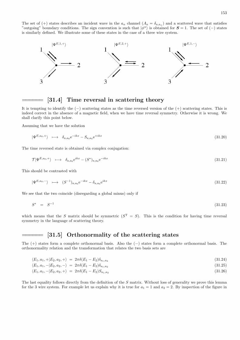
153

The set of (+) states describes an incident wave in the aα channel (Aa = δa,aα) and a scattered wave that satisfies”outgoing” boundary conditions. The sign convention is such that |φα〉 is obtained for S = 1. The set of (−) statesis similarly defined. We illustrate some of these states in the case of a three wire system.

|ΨE,1,+〉 |ΨE,2,+〉 |ΨE,1,−〉

====== [31.4] Time reversal in scattering theory

It is tempting to identify the (−) scattering states as the time reversed version of the (+) scattering states. This isindeed correct in the absence of a magnetic field, when we have time reversal symmetry. Otherwise it is wrong. Weshall clarify this point below.

Assuming that we have the solution

|ΨE,a0,+〉 7−→ δa,a0e−ikx − Sa,a0

e+ikx (31.20)

The time reversed state is obtained via complex conjugation:

T |ΨE,a0,+〉 7−→ δa,a0eikx − (S∗)a,a0e−ikx (31.21)

This should be contrasted with

|ΨE,a0,−〉 7−→ (S−1)a,a0e−ikx − δa,a0

eikx (31.22)

We see that the two coincide (disregarding a global minus) only if

S∗ = S−1 (31.23)

which means that the S matrix should be symmetric (ST = S). This is the condition for having time reversalsymmetry in the language of scattering theory.

====== [31.5] Orthonormality of the scattering states

The (+) states form a complete orthonormal basis. Also the (−) states form a complete orthonormal basis. Theorthonormality relation and the transformation that relates the two basis sets are

〈E1, a1,+|E2, a2,+〉 = 2πδ(E1 − E2)δa1,a2(31.24)

〈E1, a1,−|E2, a2,−〉 = 2πδ(E1 − E2)δa1,a2 (31.25)

〈E1, a1,−|E2, a2,+〉 = 2πδ(E1 − E2)Sa1,a2 (31.26)

The last equality follows directly from the definition of the S matrix. Without loss of generality we prove this lemmafor the 3 wire system. For example let us explain why it is true for a1 = 1 and a2 = 2. By inspection of the figure in

154

a previous section we see that the singular overlaps comes only from the first and the second channels. Disregardingthe ”flux” normalization factor the singular part of the overlap is

〈E1, 1,−|E2, 2,+〉∣∣∣singular

=

∫ ∞0

[− eikr

]∗[− S12e+ik0r

]dr +

∫ ∞0

[(S−1)21e−ikr

]∗[e−ik0r

]dr (31.27)

=

∫ ∞0

S12e−i(k−k0)rdr +

∫ 0

−∞S12e−i(k−k0)rdr = 2πδ(k − k0)S12

where is the second line we have changed the dummy integration variables of the second integral from r to −r,and used (S−1)∗21 = S12. If we restore the ”flux normalization” factor we get the desired result. One can wonderwhat about the non-singular contributions to the overlaps. These may give, and indeed give, an overlap that goeslike 1/(E ± E0). But on the other hand we know that for E 6= E0 the overlap should be exactly zero due to theorthogonality of states with different energy (the Hamiltonian is Hermitian). If we check whether all the non-singularoverlaps cancel, we find that this is not the case. What is wrong? The answer is simple. In the above calculation wedisregarded a non-singular overlap which is contributed by the scattering region. This must cancel the non-singularoverlap in the outside region because as we said, the Hamiltonian is Hermitian.

====== [31.6] Getting the S matrix from the T matrix

In this section we present a relation between the S matrix and the T matrix. The derivation of this relations goesas follows: On the one hand we express the overlap of the ingoing and outgoing scattering states using the S matrix.On the other hand we express it using the T matrix. Namely,

〈ΨE1,a1,−|ΨE2,a2,+〉 = 2πδ(E1 − E2)Sa1a2 (31.28)

〈ΨE1,a1,−|ΨE2,a2,+〉 = 2πδ(E1 − E2) (δa1a2− iTa1a2

)

By comparing the two expressions we deduce the relation between the S matrix and the T matrix:

Sa1a2 = δa1a2 − iTa1a2 (31.29)

or in abstract notation S = 1− iT . Another way to re-phrase this relation is to say that the S matrix can be obtainedfrom the matrix elements of an S operator:

〈φE1,a1 |S|φE2,a2〉 = 2πδ(E1 − E2)Sa1a2(31.30)

where the S operator is the evolution operator in the interaction picture. Within the framework of the time dependentapproach to scattering theory the latter relation is taken as the definition for the S matrix. The two identities that weprove in the previous and in this section establish that the time-independent definition of the S matrix and the timedependent approach are equivalent. The rest of this section is dedicated to the derivation of the T matrix relation.

First order derivation.– We recall that the scattering states are defined as the solution of HΨ = EΨ and theycan be expressed as

ΨE2,a2,+ =(1 +G+

0 (E2)V + ...)φE2,a2 (31.31)

ΨE1,a1,− =(1 +G−0 (E1)V + ...

)φE1,a1 (31.32)

Hence

〈ΨE1,a1,−|ΨE2,a2,+〉 = 〈φE1,a1 |φE2,a2〉+ 〈φE1,a1 |V G+0 (E1) +G+

0 (E2)V |φE2,a2〉+ ... (31.33)

= 〈φE1,a1 |φE2,a2〉+

[1

E1 − E2 + i0+

1

E2 − E1 + i0

]〈φE1,a1 |V |φE2,a2〉+ ... (31.34)

= 2πδ(E1 − E2)δa1a2− i2πδ(E1 − E2)〈φE1,a1 |V |φE2,a2〉+ ... (31.35)

155

Full derivation.– We recall that the scattering states can be expressed as

ΨE2,a2,+ = (1 +G+(E2)V )φE2,a2 =

(1 +

1

E2 −H+ i0V

)φE2,a2 (31.36)

ΨE1,a1,− = (1 +G−(E1)V )φE1,a1 =

(1 +

1

E1 −H0 − i0T (E1)†

)φE1,a1 (31.37)

where the last equality relays on GV = G0T . In the following calculation we use the first identity for the ”ket”, andafter that the second identity for the ”bra”:

⟨ΨE1,a1,−|ΨE2,a2,+

⟩=

⟨ΨE1,a1,−

∣∣∣∣1 +1

E2 −H+ i0V

∣∣∣∣φE2,a2

⟩(31.38)

=

⟨ΨE1,a

−1

∣∣∣∣1 +1

E2 − E1 + i0V

∣∣∣∣φE2,a2

⟩=

⟨φE1,a1

∣∣∣∣[1 + T (E1)1

E1 −H0 + i0

] [1 +

V

E2 − E1 + i0

]∣∣∣∣φE2,a2

⟩=

⟨φE1,a1

∣∣∣∣[1 +T (E1)

E1 − E2 + i0

]∣∣∣∣φE2,a2

⟩+

⟨φE1,a1

∣∣∣∣V + T (E1)G+0 (E1)V

E2 − E1 + i0

∣∣∣∣φE2,a2

⟩=

⟨φE1,a1

∣∣∣∣1 +T (E1)

E1 − E2 + i0

∣∣∣∣φE2,a2

⟩+

⟨φE1,a1

∣∣∣∣ T (E1)

E2 − E1 + i0

∣∣∣∣φE2,a2

⟩= 2πδ(E1 − E2)δa1a2 − i2πδ(E1 − E2)

⟨φE1,a1 |T (E1)|φE2,a2

⟩where before the last step we have used the relation V + TG0V = T .

====== [31.7] Subtleties in the notion of cross section

Assume that we have a scattering state Ψ. We can write it as a sum of ”ingoing” and ”outgoing” waves or as a sumof ”incident” and ”scattered” waves. This is not the same thing!

Ψ = Ψingoing + Ψoutgoing (31.39)

Ψ = Ψincident + Ψscattered

The ”incident wave” is a ”free wave” that contains the ”ingoing” wave with its associated ”outgoing” component.It corresponds to the H0 Hamiltonian. The ”scattered wave” is what we have to add in order to get a solution tothe scattering problem with the Hamiltonian H. In the case of the usual boundary conditions it contains only an”outgoing” component.

ΨoutgoingΨ ingoingΨscattered

Ψ incident

Below is an illustration of the 1D case where we have just two directions of propagation (forwards and backwards):

156

Ψ ingoing

ΨoutgoingΨoutgoing Ψscattered

Ψ incident

The S matrix gives the amplitudes of the outgoing wave, while the T = i(1 − S) matrix gives the amplitudes of thescattered component (up to a phase factor). Let us consider extreme case in order to clarify this terminology. If wehave in the above 1D geometry a very high barrier, then the outgoing wave on the right will have zero amplitude.This means that the scattered wave must have the same amplitude as the incident wave but with the opposite sign.

In order to define the ”cross section” we assume that the incident wave is a density normalized (ρ = 1) plane wave.This is like having a current density J = ρvE . If we regard the target as having some ”area” σ then the scatteredcurrent is

Iscattered = (ρvE)× σ (31.40)

It is clear from this definition that the units of the cross section are [σ] = Ld−1. In particular in 1D geometry the”differential cross section” into channel a, assuming an incident wave in channel a0 is simply

σa = |Ta,a0|2 (31.41)

and by the ”optical theorem” the total cross section is

σtotal = −2Im[Ta0,a0 ] (31.42)

The notion of ”cross section” is problematic conceptually because it implies that it is possible for the scattered flux tobe larger than the incident flux. This is most evident in the 1D example that we have discussed above. We see thatthe scattered wave is twice the incident wave, whereas in fact the forward scattering cancels the outgoing componentof the incident wave. Later we calculate the cross section of a sphere in 3D and get twice the classical cross section(2πa2). The explanation is the same - there must be forward scattering that is equal in magnitude (but opposite insign) to the outgoing component of the incident wave in order to create a ”shadow region” behind the sphere.

====== [31.8] The Wigner time delay

A given element of the S matrix can be written as

Sab =√geiθ (31.43)

where 0 < g < 1 is interpreted as either transmission or reflection coefficient, while θ is called phase shift. The crosssection is related to g while the Wigner time delay that we discuss below is related to θ. The Wigner time delay isdefined as follows:

τdelay(E) = ~dθ

dE(31.44)

Consider for example the time delay in the case of a scattering on a “hard” sphere of radius R. We shall see that insuch case we have a smooth energy dependence θ ≈ −2kR and consequently we get the expected result τ ≈ −2R/vE .On the other hand we shall consider the case of a scattering on a shielded well. If the energy is off resonance we getthe same result τ ≈ −2R/vE . But if E is in the vicinity of a resonance, then we can get a very large (positive) timedelay τ ∼ ~/Γr, where Γr is the so called “width” of the resonance. This (positive) time delay reflects ”trapping” andit is associated with an abrupt variation of the cross section as discussed in a later section.

157

Let us explain the reasoning that leads to the definition of the Wigner time delay. For this purpose we consider thepropagation of a Gaussian wavepacket in a given channel:

Ψ(x) =

∫dk e−σ

2(k−k0)2 √g exp [i (k(x− x0) + θ − Et)] (31.45)

where both g and θ and E are functions of k. In order to determine the position x of the wavepaket we use thestationary phase approximation. Disregarding the Gaussian envelope, and regarding g as constant at the energyrange of interest, most of contribution to the dk integral comes from the k region where the phase is stationary. Thisleads to

x− x0 +dθ

dk− dE

dkt = 0 (31.46)

The position x of the wavepacket is determined by the requirement that the above equation should have a solutionfor k ∼ k0. Thus we get

x = x0 + vgroup × (t− τdelay) (31.47)

where vgroup = (dE/dk) is the group velocity for k = k0 and τdelay is the Wigner time delay as defined above. Howthis is related to a scattering problem? Consider for example scattering on one dimensions where we have ”left” and”right” channels. Assume that the wavepacket at t = 0 is an undistorted Gaussian with θ = 0. The initial wavepacketis centered on the ”left” around x = x0 with momentum k = k0. We would like to know how x evolves with timebefore and after the scattering. Say that we observe the transmitted part of the wavepacket that emerges in the”right” channel. Following the above analysis we conclude that the effect of introducing θ 6= 0 is the Wigner timedelay.

====== [31.9] The Friedel phase and the DOS

The issue that we discuss in this section is how to determine the number N (E) of energy levels in the scatteringregion if we know how the S matrix depends on the energy E. This would be the number of no interacting Fermionsthat can be accommodated there at zero temperature. More precisely what we can extract from S(E) is the densityof states %(E) in the scattering region. To have a clear idea of the physical picture it is best to imagine a single leadsystem, where the lead is a waveguide with M modes, and the “depth” of the scattering region is L. In such system

%(E) ∼ M× vEπ

L∼ M× τdelay (31.48)

where τdelay ∼ L/vE is the semiclassical estimate for the time delay. We shall see that the so called Friedel-sum-ruleis merely a refinement of the latter formula. In complete analogy with the Wigner formula, that express τdelay as theE derivative of the scattering phase shift, we are going to express %(E) as the E derivative of the “Friedel phase”.

The most illuminating way to define the energy levels of the scattering region is to impose Dirichlet boundary conditionat the r = 0 section. This leads to the equation (say for 3 modes):

S

A1

A2

A3

=

A1

A2

A3

(31.49)

This equation has a non-trivial solution if and on if

det(S(E)− 1

)= 0 (31.50)

Form this condition we can extract the eigen-energies. Recall that the S matrix is unitary. Therefore its M complexeigenvalues eiθr are located on a circle. We get zero determinant in the above equation each time that one of the

158

eigen-phases cross through θ = 0. Thus the mean level spacing is simply 2π/M divided by the average “velocity”dθ/dE. This leads to

%(E) =1

2π

(dθE

dE

)=

1

2πitrace

(dS

dES†)

(31.51)

where the Friedel phase is θE =∑r θr. The last equality is easily derived by calculating the trace in the basis in

which S is diagonal.

A straightforward generalization of the above considerations allow to calculate the number of fermions that are emittedfrom the scattering region if a parameter X is being varied very very slowly such that at any moment we have zerotemperature occupation. The result can be written as dN = −GdX where

G =1

2πitrace

(dS

dXS†)

(31.52)

The further generalization of this relation to multi-lead geometry has been discussed by Brouwer following the workof Buttiker Pretre and Thomas, and is known as the scattering approach to quantum pumping.

====== [31.10] Phase shifts and resonances

If we have only one wire (hence one channel) the S matrix is 1× 1, and accordingly we can write

S00 = exp[i2δ0(E)] (31.53)

T00 = −eiδ02 sin(δ0) (31.54)

where δ0(E) is known as the phase shift. If the scattering potential is short range one can use a matching procedure inorder to determine the phase shift. This will be discussed in the next lecture. Another possibility is to use perturbationtheory via the T matrix formalism:

T00 = V00 + (V GV )00 = Born expansion (31.55)

It is essential to calculate the matrix elements using properly flux-normalized free waves:

|φE〉 =1√vE

e−ikEr − 1√vE

e+ikEr = −i 1√vE

2 sin(kEr) (31.56)

There are two limiting cases of particular interest.

• First order non-resonant scattering by a weak potential V

• Resonant scattering which is dominated by a single pole of G

In the case of scattering by a weak potential we can use the first order Born approximation for the T matrix:

T00 ≈ V00 = 〈φE |V |φE〉 =4

vE

∫ ∞0

V (r) (sin(kEr))2dr (31.57)

The assumption of weak scattering implies δ0 1, leading to the first order Born approximation for the phase shift:

δBorn0 ≈ − 2

vE

∫ ∞0

V (r) (sin(kEr))2dr (31.58)

159

This formula is similar to the WKB phase shift formula. It has a straightforward generalization to any ` which wediscuss in the context of spherical geometry. We note that we have manged above to avoid the standard lengthyderivation of this formula, which is based on the Wronskian theorem (Messiah p.404).

The other interesting case is resonant scattering where

T00 ≈ (V GV )00 =〈φE |V |r〉〈r|V |φE〉E − Er + i(Γr/2)

(31.59)

From the optical theorem 2Im[T00] = −|T00|2 we can deduce that the numerator, if it is real, must equal Γr. Thus wecan write this approximation in one of the following equivalent ways:

T00 =Γr

E − Er + i(Γr/2)(31.60)

S00 =E − Er − i(Γr/2)

E − Er + i(Γr/2)(31.61)

tan(δ`) = − Γr/2

E − Er(31.62)

Note that if the optical theorem were not satisfied by the approximation we would not be able to get a meaningfulexpression for the phase shift. In order to prove the equivalence of the above expressions note that δ0 can be regardedas the polar phase of the complex number z = (E−Er)− i(Γr/2).

The Wigner time delay is easily obtained by taking the derivative of δ0(E) with respect to the energy. This gives aLorentzian variation of τdelay as a function of (E−Er). The width of the Lorentzian is Γr, and the time delay at thecenter of the resonance is of order ~/Γr.

160

[32] Scattering in quasi 1D geometryIn this lecture we consider various scattering problems is which the radial functions are exp(±ikar), where a is thechannel index. In order to find a scattering solution we have to use a matching procedure. Namely the ingoing andoutgoing free wave solutions should match an interior solution within the scattering region. This requirement imposesa boundary condition that relates the wavefunction amplitude and its derivative on the boundary. The simplestexample for this class of systems is a network that consists of M semi 1D wires that are connected at one junction.The problem of s-scattering (` = 0) in spherical geometry is formally the same asM=1 ”semi 1D wire” problem. Weshall discuss the general case (any `) in a later lecture. The 1D scattering problem on a line, where we have ”left”and ”right” leads, is formally an M=2 ”semi 1D wire” system. Then it is natural to consider less trivial M channelsystems that can be regarded as generalizations of the 1D problem, including scattering in waveguides and multi-leadgeometries. Also inelastic scattering in 1D can be formally re-interpreted as an M channel ”semi 1D wire” problem.

====== [32.1] The matching procedure

In this section we would like to outline a procedure for finding an exact result for the phase shift is quasi 1D onechannel geometry. This procedure will allow us to analyze s-scattering by “hard” spheres as well as by “deep” wells.The key assumption is that we have a finite range potential which is contained within the region r < R. The boundaryof the scattering region at r = R is fully characterized by the logarithmic derivative k0(E). The definition of the latteris as follows: given the energy E, one finds the regular solution ψ(r) of the Schrodinger equation in the interior (r ≤ R)region; Typically this solution is required to satisfy Dirichlet boundary conditions at the origin r = 0; Once the regularsolution is known, the logarithmic derivative at the boundary is calculated as follows:

k0 =

[1

ψ(r)

dψ(r)

dr

]r=R

(32.1)

The derivative should be evaluated at the outer side of the boundary. For each problem k0(E) should be evaluatedfrom scratch. But once it is known we can find both the E < 0 bound states and the E > 0 scattering states of thesystem. It is useful the consider the simplest example: square well of radius R that has depth |V0|. The regularsolution in the interior region is Ψ(r) ∝ sin(αinr), and accordingly the logarithmic derivative at the boundary is

k0(E) = αin cot(αinR), where αin =√

2m(E + |V0|) (32.2)

Finding the bound states: In the case of a bound state the wavefunction at the outside region is ψ(r) ∝ exp(−αEr).The matching with the interior solution gives the equation

k0(E) = −αE where αE =√

2m|E| (32.3)

This equation determines the eigen-energies of the system. In order to have bound states k0 should become negative.This is indeed the case with square well as |V0| being increased. It should be opposed with the case of a square barrier.

Finding the scattering states: For positive energies we look for scattering states. The scattering solution in theoutside region is

Ψ(r) = Ae−ikEr −BeikEr = A(e−ikEr − ei2δ0eikEr) = C sin(kEr + δ0) (32.4)

where δ0 is the phase shift. The matching with the interior solution gives the equation

kE cot(kER+ δ0) = k0 (32.5)

This equation can be written as tan(δ0−δ∞0 ) = kE/k0, where δ∞0 = −kER is the solution for “hard sphere scattering”.Thus the explicit solution for the phase shift is

δ0 = δ∞0 + arctan(kE

k0

) (32.6)

161

It is clear that in practical problems the boundary r = R is an arbitrary radius in the ”outside” region. It is mostnatural to extrapolate the outside solution into the the region r < R as if the potential there is zero. Then it ispossible to define the logarithmic derivative k0 of the extrapolated wavefunction at r = 0. This function contains thesame information as k0, while the subtlety of fixing an arbitrary R is being avoided. From the above analysis we get

k0(E) =

[1

ψ(r)

dψ(r)

dr

]r=0

= kE cot(δ0(E)) =k0 + kE tan(kER)

kE − k0 tan(kER)(32.7)

At low energies, in the limit kE → 0, this expression takes the simpler form k0 = ((1/k0)−R)−1.

====== [32.2] Low energy scattering

Of particular interest is the long-wavelength limit, which means kER 1 where R is the radius of the scatteringregion. Then the regular solution for r ∼ R, where the potential is zero, has the form ψ(r) ∝ r − as. This implies bydefinition that for low energy δ0 = −kEas. The parameter as is called the scattering length. Given as, it follows fromthe above definition that the log derivative, referenced to the origin, is k0 = −1/as. More generally it is customaryto expand the log-derivative at the origin as follows:

k0(E) ≡ kE cot(δ0(E)) = − 1

as+

1

2rsk

2E + ... (32.8)

Thus as is merely a parameter in the expression for phase shift in the limit of low energies. If this phase shift is smallit can be expressed as δ0 = −kEas. For a sphere of radius R and potential V0 one obtains as = R in the hard spherelimit (V0 =∞). As V0 is decreased one obtains as ≈ (2/3)mR3V0. For negative V0 (“spherical well”) one obtains

as = R− (1/α) tan(αR), where α =√

2m|V0|.

At this stage we mention a common terminology that might look strange at first sight. Referring to a square wellit is clear that is |V0| is very small the potential has no bound state. We can regard such potential as a broadeneddelta function V (r) = uδ(r) that has u < 0. In such situation we have δ0 > 0 and as < 0, which should be contrastedwith hard sphere. Such u < 0 scattering potential is called “attractive”. As |V0| becomes larger it can accommodatea bound state, and it behaves like a u > 0 delta potential with δ0 < 0 and as > 0. Such scattering potential is called“repulsive”. The bound state energy of the such “repulsive” potential is determined from the matching condition thathas been discussed in the previous section, leading to

Ebound = − 1

2ma2s

(32.9)

It should be clear that this solution is meaningful provided the assumptions as R and |Ebound| < ∆ are satisfied.Here ∆ is the range within which as can be regarded as a constant.

From the definition of the scattering length it follows that for weak scattering it can be expressed as δ0 = −kEas. Ina later section we shall see that in 3D this means that the total s-scattering cross section is

σtotal =4π

k2E

sin2(δ0) ≈ 4πa2s (32.10)

A delta function V (x) = u δ3(x) in 3D has a zero total cross section. Still from the first order Born approximationfor the T matrix we get as an artifact

σtotal = 4π( m

2πu)2

(32.11)

It is therefore common to describe an s-scatterer that is characterize by a scattering length as, as a delta scattererwith u = 2πas/m. One should be very careful with the latter point of view.

162

====== [32.3] Inelastic scattering by a delta scatterer

We consider inelastic scattering on a delta scatterer in one dimension [arXiv:0801.1202]

H =p2

2m+Qδ(x) +Hscatterer (32.12)

The scatterer is assumed to have energy levels n with eigenvalues En. It should be clear that inelastic scattering ofa spinless particle by a multi level atom is mathematically equivalent to inelastic scattering of a multi level atom bysome static potential. Outside of the scattering region the total energy of the system (particle plus scatterer) is

E = εk + En (32.13)

We look for scattering states that satisfy the equation

H|Ψ〉 = E|Ψ〉 (32.14)

The scattering channels are labeled as

n = (n0, n) (32.15)

where n0 = left,right. We define

kn =√

2m(E − En) for n ∈ open (32.16)

αn =√−2m(E − En) for n ∈ closed (32.17)

later we use the notations

vn = kn/m (32.18)

un = αn/m (32.19)

and define diagonal matrices v = diagvn and u = diagun. The channel radial functions are written as

R(r) = Ane−iknr +Bne+iknr for n ∈ open (32.20)

R(r) = Cne−αnr for n ∈ closed (32.21)

where r = |x|. Next we derive expression for the 2N × 2N transfer matrix T and for the 2N × 2N scattering matrixS, where N is the number of open modes. The wavefunction can be written as

Ψ(r, n0, Q) =∑n

Rn0,n(r)χn(Q) (32.22)

The matching equations are

Ψ(0, right, Q) = Ψ(0, left, Q) (32.23)

1

2m[Ψ′(0, right, Q) + Ψ′(0, left, Q)] = QΨ(0, Q) (32.24)

The operator Q is represented by the matrix Qnm that has the block structure

Qnm =

(Qvv QvuQuv Quu

)(32.25)

163

For sake of later use we define

Mnm =

(1√vQvv

1√v

1√vQvu

1√u

1√uQuv

1√v

1√uQuu

1√u

)(32.26)

The matching conditions lead to the following set of matrix equations

AR +BR = AL +BL (32.27)

CR = CL (32.28)

−iv(AR −BR +AL −BL) = 2Qvv(AL +BL) + 2QvuCL (32.29)

−u(CR + CL) = 2Quv(AL +BL) + 2QuuCL (32.30)

from here we get

AR +BR = AL +BL (32.31)

AR −BR +AL −BL = i2(v)−1Q(AL +BL) (32.32)

where

Q = Qvv −Qvu1

(u+Quu)Quv (32.33)

The set of matching conditions can be expressed using a transfer matrix formalism that we discuss in the nextsubsection, where

M =1√vQ 1√

v= Mvv −Mvu

1

1 +MuuMuv (32.34)

====== [32.4] Finding the S matrix from the transfer matrix

The set of matching conditions in the delta scattering problem can be written as

(BRAR

)= T

(ALBL

)(32.35)

where An =√vnAn and Bn =

√vnBn. The transfer 2N × 2N matrix can be written in block form as follows:

T =

(T++ T+−T−+ T−−

)=

(1− iM −iMiM 1 + iM

)(32.36)

The S matrix is defined via(BLBR

)= S

(ALAR

)(32.37)

and can be written in block form as

Sn,m =

(SR STST SR

)(32.38)

164

A straightforward elimination gives

S =

(−T−1−−T−+ T−1

−−T++−T−+T

−1−−T+− T+−T

−1−−

)=

((1 + iM)

−1 − 1 (1 + iM)−1

(1 + iM)−1

(1 + iM)−1 − 1

)(32.39)

Now we can write expressions for SR and for ST using the M matrix.

ST =1

1 + iM= 1− iM−M2 + iM3 + ... (32.40)

SR = ST − 1 (32.41)

====== [32.5] Elastic scattering by a delta in a waveguide

The elastic scattering of a spinless particle by a regularized delta scatterer in a waveguide is mathematically the sameproblem as that of the previous section. We have

Q = cδ(y − y0) (32.42)

for which

Qnm = c

∫χnδ(y − y0)χmdy = c χn(y0)χm(y0) (32.43)

Given the total energy we define

Mnm =1√|vn|

Qnm1√|vm|

≡(Mvv Mvu

Muv Muu

)(32.44)

Regularization means that one impose a cutoff on the total number of coupled channels, hence M is a finite (truncated)matrix. Using the formula for inverting a matrix of the type 1− aa†, we first obtain M and then obtain

SR =iMvv

1 + i trace[Mvv] + trace[Muu](32.45)

Let us consider what happens as we change the total energy: Each time that a new channels is opened the scatteringcross section becomes zero. Similarly, if we remove the regularization we get zero scattering for any energy becauseof the divergent contribution of the closed channels.

====== [32.6] Transmission through a tight-binding network

Consider a network that consists of N sites and described by Hamiltonian H′. We can attach a lead to a site of thenetwork, or in general we attach several leads to different points. We would like to calculate the S matrix in thisconfiguration. For this purpose we apply the T matrix formalism, combined with the ”P+Q” formalism where ”P” isthe network and ”Q” are the leads.

The lead is regarded as a chain of sites (x = 1, 2, 3, ...) with hopping amplitude −c0. Accordingly a free ”wave” withwavenumber k has energy and velocity as follows:

ε = −2c0 cos(k) (32.46)

v = 2c0 sin(k), mass ≡ 1/(2c0) (32.47)

165

The flux-normalized free wave in a disconnected lead is

ϕ(x) =2√v

sin(kx), Note: ϕ(1) =

√v

c0(32.48)

The Green function due a source at the first site is

Glead(x|1) = − 1

c0eikx Note: G(1|1) =

ε− iv2c20

(32.49)

The hopping amplitude between the x = 1 site of the lead that is labeled as a, and a contact point the network thatis labeled as na, will be denoted −cγ . Later we shall define the dimensionless coupling parameter γ = (cγ/c0)2. If wehave M leads it is convenient to pack the couplings in a rectangular M ×N contact matrix Q that is composed ofzeros and ones, such that Va,n = −cγQa,n. The Green function of the network can be calculated using the ”P+Q”expression

G(n|m) =

[1

ε−H0 − V †GleadV

]n,m

=

[1

ε−H0 − γ2 (ε− iv)Q†Q

]n,m

(32.50)

The scattering matrix is expressed as S = 1− iT , where the T matrix elements are

Ta,b = =⟨ϕa∣∣V GV †∣∣ϕb⟩ =

[γv

ε−Heff + iγv2 Q†Q

]na,nb

(32.51)

where na and nb are the contact sites of lead a and lead b, and the definition of Heff is implied from the expressionfor G(n|m). Note that the Q†Q term implies that the on-site potential at the contact sites becomes complex.

Assume that the network represents a 1D wire segment to which leads are attached at the endpoint. Ideal contactscorresponds to γ = 1. It is instructive to consider the continuum limit of the T matrix expression for such a setup. Thislimit corresponds to small k at the bottom of the band where ε ≈ −2c0. One observes that the effective Hamiltonianbecomes

Heff = H0 − c0Q†Q (32.52)

This Hamiltonian corresponds to Neumann boundary conditions. The reasoning is as follows: If we place a negativedelta −[1/(2ma)]δ(x−a) at an infinitesimal distance a from the endpoint x = 0 of the segment, it forces the derivativeto be zero. In a tight-binding model this is like having a potential −c0 at the first site.

====== [32.7] Transmission through a cavity

Consider a cavity to which a lead is attached. We would like to calculate the S matrix in this configuration. Onepossibility is to take the continuum limit of the network model that we have solved in the previous section. This leadsto the so-called Weidenmuller formula:

S = 1 − iWGW = 1 − iW1

E −Heff + i(W †W/2)W † (32.53)

where Heff is the Hamiltonian of the cavity with Neumann boundary conditions on the surface of the scattering region.It is convenient to find a complete set ϕ(n)(x) of cavity eigenfunctions. Then the expression for the contact matrixtakes the form

Wa,n =√va

∫χa(s)ϕ(n)(x(s)) ds (32.54)

166

where χa(s) are the channel functions and s is the transverse coordinate. Conventionally the Weidenmuller formulais derived from the so called R matrix formalism, which we outline below.

The Fisher-Lee relation.– Before we go on it is appropriate to point out the duality between the Weidenmullerformula and the Fisher-Lee relation. The latter expresses the Green function G(s|s0) using the S matrix as given. Thesurface coordinates s and s0 indicate points x(s) and x(s′) on the boundary of the scattering region. The standardderivation goes as follows [Datta]: We place a source at the lead and use the S matrix to define the boundaryconditions on the surface x(s) of the scattering region. We solve for the outgoing amplitudes and find that

G(s|s0) = i∑ab

1√vaχa(s) (S − 1)ab

1√vbχb(s0) (32.55)

This relation can be inverted:

Sab = δab − i√vavb

∫χa(s) G(s|s0) χb(s0) dsds0 ≡

[1− iWGW †

]a,b

(32.56)

The latter expression has the same expected structure that is anticipated from T matrix theory, and therefore shouldbe equivalent to the Weidenmuller formula. Inserting a complete basis of cavity eigenstates for the representation ofthe Green function, the integral over s becomes a sum over n, and the definition of W is implied. Still this perspectivedoes not provide a practical procedure for the choice of the n basis, and for the evaluation of Gn,n′ .

The R matrix formalism.– We would like to describe a formulation that opens the way for a powerful numericalprocedure for finding the S matrix of a cavity-lead system. The idea is to reduce the scattering problem to a boundstate problem by chopping the leads. It can be regarded as a generalization of the one-dimensional phase shift methodwhere the outer solution is matched to an interior solution. The latter is characterized by its log derivative on theboundary. In the same spirit the R matrix is defined through the relation

Ψ(s) =

∫R(s, s′)∂Ψ(s′) ds′ (32.57)

If we decompose this relation into channels we can rewrite it as

Ψa =∑b

Rab∂Ψb (32.58)

Expressing Ψa and ∂Ψa as the sum and the difference of the ingoing and the outgoing amplitudes Aa and Ba, onefinds a simple relation between the R matrix and the S matrix:

Rab = i1√kakb

(1− S1 + S

)ab

(32.59)

The inverse relation is

S =1 + i

√kR√k

1− i√kR√k

(32.60)

From the Green theorem it follows that

R(s, s′) = − ~2

2mGN (s′|s) (32.61)

167

where GN is the Green function of the interior with Neumann boundary conditions on the surface of the scatteringregion. If we find a complete set of interior eigenfunctions then

GN (s′|s) =∑n

ϕ(n)(s′)ϕ(n)(s)

E − En(32.62)

and consequently

Rab = −1

2

∑n

(Wan√ka

)1

E − En

(Wbn√kb

)(32.63)

The corresponding result for the S matrix is obtained by expanding (1 + x)/(1− x) = 1 + 2(...) with the identificationof (...) as the diagrammatic expression of the resolvent. This leads to the Weidenmuller formula.

168

[33] Scattering in a spherical geometryOf special interest is the scattering problem in 3D geometry. We shall consider in this lecture the definitions of thechannels and of the S matrix for this geometry. Later analyze in detail the scattering by a spherically symmetrictarget. In the latter case the potential V (r) depends only on the distance from the origin. In order to find thescattering states we can perform separation of variables, where ` and m are good quantum numbers. In the (`,m)subspace the equation for the radial function u(r) = rR(r) reduces to a one dimensional Schrodinger equation on the0 < r <∞ axis. To avoid divergence in R(r) we have to use the boundary condition u(0) = 0, as if there is an infinitewall at r = 0.

Most textbooks focus on the Coulomb interaction V (r, θ, ϕ) = −α/r for which the effective radial potential isVeff(r) = −α/r + β/r2. This is an extremely exceptional potential because of the following:

• There is no centrifugal barrier.• Therefore there are no resonances with the continuum.• It has an infinite rather than a finite number of bound states.• The frequencies of the radial and the angular motions are degenerate.• Hence there is no precession of the Kepler ellipse.

We are going to consider as an example scattering on a spherical target which we call either ”sphere” or ”well”.The parameters that characterize the sphere are its radius a, the height of the potential floor V , and optionally the”thickness” the shielding U . Namely,

V (r, θ, ϕ) = VΘ(a− r) + Uδ(r − a) (33.1)

Disregarding the shielding the effective radial potential is Veff(r) = VΘ(a− r) + β/r2. We consider first hard sphere(V0 =∞) and later on the scattering on a spherical well (V0 < 0). The effective potential for 3 representative valuesof V is illustrated in panels (a)-(b)-(c) of the following figure. In panels (d) we illustrate, for sake of comparison, theeffective potential in case of a Coulomb interaction.

effV (r)

2

22mal

2

22mal

2

22mal

2

22mal

V0

a a

0V <0

0+V <0 −a/r + b/r 2

Classically it is clear that if the impact parameter b of a particle is larger than the radius a of the scattering region

169

then there is no scattering at all. The impact parameter is the distance of the particle trajectory (extrapolated asa straight line) from form the scattering center. Hence its angular momentum is ` = mvEb. Thus the semiclassicalcondition for non-negligible scattering can be written as

b < a ⇔ ` < kEa ⇔ `2

2ma2< E (33.2)

The last version is interpreted as the condition for reflection from the centrifugal barrier (see Fig). In the channelswhere the semiclassical condition is not satisfied we expect negligible scattering. (no phase shift). This semiclassicalexpectation assumes that the ”forbidden” region is unaccessible to the particle, hence it ignores the possibility oftunneling and resonances that we shall discuss later on. Whenever we neglect the latter possibilities, the scatteringstate is simply a free wave which is described by the spherical Bessel function j`(kEr). For kEr ` this sphericalBessel function is exponentially small due to the centrifugal barrier, and therefore it is hardly affected by the presenceof the sphere.

====== [33.1] The spherical Bessel functions

Irrespective of whether the scattering potential is spherically symmetric or not the Schrodinger equation is separableoutside of the scattering region. This means that we can expand any wavefunction that satisfies HΨ = EΨ in theoutside region as follows:

Ψ(x) =∑`,m

R`,m(r)Y `m(θ, ϕ) (33.3)

The channel index is a = (`,m) while Ω = (θ, ϕ) is analogous to the s of the 2D lead system. The Y `m are the channelfunctions. In complete analogy with the case of 1D geometry we can define the following set of functions:

h+` (kEr)↔ eikEr (33.4)

h−` (kEr)↔ e−ikEr

j`(kEr)↔ sin(kEr)

n`(kEr)↔ cos(kEr)

Note that the right side equals the left side in the special case ` = 0, provided we divide by r. This is because thesemi-1D radial equation becomes literally the 1D Schrodinger equation only after the substitution R(r) = u(r)/r.

In what follows we use Messiah convention p.489. Note that other textbooks may use different sign convention. Therelation between the functions above is defined as follows:

h±` = n`(kr)± ij`(kr) (33.5)

We note that the jn(r) are regular at the origin, while the nn(r) are singular at the origin. Therefore only the formerqualify as global ”free waves”. The l = 0 functions are:

j0(kr) =sin(kr)

kr(33.6)

n0(kr) =cos(kr)

kr

170

The asymptotic behavior for kr `+1 is:

h±` (kr) ∼ (∓i)` e±ikr

kr(33.7)

n`(kr) ∼cos(kr − π

2 `)

kr

j`(kr) ∼sin(kr − π

2 `)

kr

The short range kr `+1 behavior is:

n`(kr) ≈ (2l − 1)!!

(1

kr

)`+1 [1 +

1

2(2l − 1)(kr)2 + . . .

](33.8)

j`(kr) ≈(kr)`

(2l + 1)!!

[1− 1

2(2l + 3)(kr)2 + . . .

]

====== [33.2] Free spherical waves

On the energy shell we write the radial wavefunctions as

R`m(r) = A`mRE,`m,−(r)−B`mRE,`,m,+(r) (33.9)

where in complete analogy with the 1D case we define

RE,`m,±(r) =kE√vE

h±` (kEr) (33.10)

The asymptotic behavior of the spherical Hankel functions is (∓i)`e±ikEr/(kEr). From this follows that the flux of theabove radial functions is indeed normalized to unity as required. Also the sign convention that we use for RE,`m,±(r)is appropriate because the free waves are indeed given by

|φE,`m〉 = [Rlm−(r)−Rlm+(r)]Y `m(θ, ϕ) = −i kE√vE

2j`(kEr)Y`m(θ, ϕ) (33.11)

This spherical free wave solution is analogous to the planar free wave |φE,Ω〉 7→ eikE~nΩ·~x. If we decide (without loss ofgenerality) that the planar wave is propagating in the z direction, then we can use the following expansion in orderto express a planar wave as a superposition of spherical waves:

eikEz =∑`

(2`+ 1) (i)` P`(cos(θ)) j`(kEr) (33.12)

We note that we have only m = 0 basis functions because there is no dependence on the angle ϕ. In different phrasingone may say that a plane wave that propagates in the z direction has Lz = 0 angular momentum. Using the identity

Y `0 =

√2`+ 1

4πP`(cos(θ)) (33.13)

we can write

eikEz =∑`,m=0

√(2l + 1)π (i)`+1

√vEkE

φE,`,m(r, θ, ϕ) (33.14)

171

which makes it easy to identify the ingoing and the outgoing components:

(eikz)ingoing =∑`m

A`mY`m(θ, ϕ)R`m−(r) (33.15)

(eikz)outgoing = −∑`m

B`mY`m(θ, ϕ)R`m+(r)

where

B`m = A`m = δm,0√

(2l + 1)π (i)`+1

√vEkE

(33.16)

This means that the incident flux in channel (`, 0) is simply

iincident =

[π

k2E

(2`+ 1)

]vE (33.17)

The expression in the square brackets has units of area, and has the meaning of cross section. The actual cross section(see next section) contains an additional factor that express how much of the incident wave is being scattered. Themaximum fraction that can be scattered is 400% as explained in the previous section.

====== [33.3] The scattered wave, phase shifts, cross section

In the past we were looking for a solution which consists of incident plane wave plus scattered component. Namely,

Ψ(r) = eik0z + f(Ω)eikEr

r(33.18)

From the decomposition of the incident plane wave it is implied that the requested solution is

Ψingoing =∑`m

A`mY`m(θ, ϕ)R`m−(r) (33.19)

Ψoutgoing = −∑`m

B`mY`m(θ, ϕ)R`m+(r)

where

A`m = δm,0√

(2l + 1)π (i)`+1

√vEkE

(33.20)

B`m = S`m,`′m′ A`′m′

If we are interested in the scattered wave then we have to subtract from the outgoing wave the incident component.This means that in the expression above we should replace S`m,`′m′ by −iT`m,`′m′ .

Of major interest is the case where the target has spherical symmetry. In such case the S matrix is diagonal:

S`m,`′m′(E) = δ``′δmm′ e2iδ` (33.21)

T`m,`′m′(E) = −δ``′δmm′ eiδ` 2 sin(δ`)

Consequently we get

Ψscattered = −∑`m

T``√

(2`+ 1)π (i)` Y `0(θ, ϕ)h+` (r) ∼ f(Ω)

eikr

r(33.22)

172

with

f(Ω) = − 1

kE

∑`

√(2`+ 1)π T`` Y

`0(θ, ϕ) (33.23)

It follows that

σtotal =

∫|f(Ω)|2dΩ =

π

k2E

∑`

(2`+ 1)|T``|2 =4π

k2E

∑`

(2`+ 1)| sin(δ`)|2 (33.24)

By inspection of the scattered wave expression we see that the scattered flux in each of the (`,m=0) channels can bewritten as i` = σ`vE , where the partial cross section is

σ` = |T``|2 ×[(2`+ 1)

π

k2E

]= (2`+ 1)| sin(δ`)|2

4π

k2E

(33.25)

It is important to realize that the scattered flux can be as large as 4 times the corresponding incident flux. Themaximum is attained if the scattering induces a π/2 phase shift which inverts the sign of the incident wave. In suchcase the scattered wave amplitude should be twice the incident wave with an opposite sign.

====== [33.4] Finding the phase shift from T matrix theory

We can get expressions for T`` = V`` + (V GV )`` using the Born expansion, and hence to get approximations for thephase shift δ` and for the partial cross section σ`. The derivation is the same as in the quasi 1D `=0 case. Theflux-normalized free waves are

|φE`m〉 = −i kE√vE

2j`(kEr)Y`m(θ, ϕ) (33.26)

The first order result for the phase shift is

δBorn` ≈ − 2

~vE

∫ ∞0

V (r) (kErjl(kEr))2dr (33.27)

while in the vicinity of resonances we have

δ` = δ∞` − arctan

(Γr/2

E − Er

)(33.28)

where δ∞` is a slowly varying “background” phase that represent the non-resonant contribution.

There are two physical quantities which are of special interest and can be deduced from the phase shift. One is thetime delay that we already have discussed in the quasi one dimensional context. The other is the cross section:

σ`(E) = (2`+ 1)4π

k2E

| sin(δ`)|2 (33.29)

For resonant scattering the ”line shape” of the cross section versus energy is typically Breit-Wigner and more generallyof Fano type. The former is obtained if we neglect δ∞` , leading to

σ` = (2`+ 1)4π

k2E

(Γr/2)2

(E − Er)2 + (Γr/2)2(33.30)

173

We see that due to a resonance the partial cross section σ` can attain its maximum value (the so called ”unitarylimit”). If we take δ∞` into account we get a more general result which is known as Fano line shape:

σ` = (2`+ 1)4π

k2E

[sin(δ∞` )]2[ε+ q]2

ε2 + 1(33.31)

where ε = (E − Er)/(Γ/2) is the scaled energy, and q = − cot(δ∞` ) is the so called Fano asymmetry parameter.The Breit-Wigner peak is obtained in the limit q → ∞, while a Breit-Wigner dip (also known as anti-resonance) isobtained for q = 0.

====== [33.5] Scattering by a soft sphere

Assuming that we have a soft sphere (|V | is small), we would like to evaluate the phase shift using the Born approx-imation. Evidently the result makes sense only if the phase shift comes out small (δ` 1). There are two limitingcases. If ka `+1 we can use the short range approximation of the spherical Bessel function to obtain

δBorn` ≈ − 2

(2`+ 3) [(2l + 1)!!]2

mV

~2a2(ka)2`+1 (33.32)

On the other hand, if ka `+1 we can use the ”far field” asymptotic approximation of the spherical Bessel functionwhich implies [krj`(kr)]

2 ≈ [sin(kr)]2 ≈ 1/2. Then we obtain

δBorn` ≈ − 1

~vEV a = −mV

~2a2(ka)−1 (33.33)

====== [33.6] Finding the phase shift by matching

We would like to generalize the quasi one-dimensional matching scheme to any `. First we have to find the radialfunction for 0 < r < a and define the logarithmic derivative

k` =

(1

R(r)

dR(r)

dr

)r=a

(33.34)

Note that we use here R(r) and not u(r) and therefore in the ` = 0 case we get k0 = k0 − (1/a). The solution in theoutside region is

R(r) = Ah−` (kEr)−Bh+` (kEr) (33.35)

= A(h−` (kEr)− ei2δ`h+` (kEr))

= C(cos(δ`)j`(kEr) + sin(δ`)n`(kEr))

We do not care about the normalization because the matching equation involves only logarithmic derivatives:

kEcos(δ)j′ + sin(δ)n′

cos(δ)j + sin(δ)n= k` (33.36)

solving this equation for tan(δ`) we get

tan(δ`) = − k`j`(ka)− kEj′`(ka)

k`n`(ka)− kEn′`(ka)(33.37)

174

which can also be written as:

ei2δ` =

(h−`h+`

)k` − (h′−` /h

−` )kE

k` − (h′+` /h+` )kE

(33.38)

In order to go from the first expression to the second note that if tan(δ) = a/b determines the phase of a complexnumber z = a+ ib then (a+ ib)/(a− ib) = ei2δ. Thus we have expressions for the phase shift given the log derivativeof the regular solution on the boundary of the scattering region.

====== [33.7] Scattering by a hard sphere

The phase shifts for a hard sphere (V →∞) can be found from the phase shift formula of the previous section usingk` →∞, leading to

tan(δ∞` ) = − j`(kEa)

n`(kEa)(33.39)

or equivalently

ei2δ∞` =

h−(kEa)

h+(kEa)(33.40)

From the first version it is convenient to derive the result

δ∞` ≈ −1

(2`+ 1)!!(2`− 1)!!(kEa)2`+1 for ` ka (33.41)

where we have used the short range expansions j` ∝ r` and n` ∝ 1/r`+1. From the second version it is convenient toderive the result

δ∞` = − arg(h+(kEa)) ≈ −(kEa−π

2`) for ` ka (33.42)

where we have used the asymptotic expression h(r) ∼ (−ı)` eikEr/r.

Small hard sphere: In the case of a small sphere (kEa 1) we have 1 δ0 δ1 δ2 . . . and the ` = 0 crosssection is dominant

δ0 = −(kEa) (33.43)

Hence

σtotal =4π

k2

∞∑l=0

(2l + 1) sin2 (δ`) ≈4π

k2sin2 (δ0) ≈ 4πa2 (33.44)

We got a σ that is 4 times bigger than the classical one. The scattering is isotropic because only the ` = 0 componentcontributes to the scattered wave.

Large hard sphere: Now we turn to the case of a large sphere (kEa 1). We neglect all δ` for which ` > kEa. Forthe non-vanishing phase shifts we get

δ` = −(kEa) for ` = 0, 2, 4, . . . (33.45)

δ` = −(kEa) + π2 for ` = 1, 3, 5, . . .

175

hence

σtotal =4π

k2

∑`=0,2...ka

(2l + 1) sin2(kEa) +∑

`=1,3...ka

(2l + 1) cos2(kEa)

(33.46)

≈ 4π

k2

`=ka∑`=0,1...ka

(2l + 1)1

2≈ 2π

k2

∫ ka

0

2xdx =2π

k2(kEa)2 = 2πa2

This time the result is 2 times the classical result. The factor of 2 is due to forward scattering which partially cancelsthe incident wave so as to create a shadow region behind the sphere.

====== [33.8] Summary of results for scattering on a sphere

We have discussed scattering on a ”hard sphere”, on a ”deep well”, and finally on a ”soft sphere”. Now we would liketo put everything together and to draw an (a, V ) diagram of all the different regimes.

V~ hma2

2

hma2

2V~ −

V

a

EV~EBorn

ka>>1

Hard Sphere

ka<<1

Resonance

Let us discuss the various regimes in this diagram. It is natural to begin with a small sphere. A small sphere meansthat the radius is small compared with the De-Broglie wavelength (ka < 1). This means that disregarding resonancesthe cross section is dominated by s-scattering (` = 0). On the one hand we have the Born approximation and on theother hand the hard sphere result:

δBorn0 ≈ −2

3

[mV

~2a2

](ka) (33.47)

δHard0 ≈ −(ka)

Thus we see that the crossover from ”soft” to ”hard” happens at V ∼ ~2/(ma2). What about V < 0? It is clearthat the Born approximation cannot be valid once we encounter a resonance (at a resonance the phase shift becomeslarge). So we are safe as long as the well is not deep enough to contain a quasi bound state. This leads to the sufficientcondition −~2/(ma2) < V < 0. For more negative V values we have resonances on top of a ”hard sphere” behavior.Thus we conclude that for ka < 1 soft sphere means

|V | < ~2/(ma2) (33.48)

176

We now consider the case of a large sphere (ka 1). In the absence of resonances we have for small impact parameter(` ka) either the Born or the hard sphere approximations:

δBorn` ≈ − V

~vEa (33.49)

δHard` = O(1)

Also here we have to distinguish between two regimes. Namely, for ka 1 soft sphere means

|V | < ~vE/a (33.50)

If this condition breaks down we expect to have a crossover to the Hard sphere result. However, one should be awarethat if V < E, then one cannot trust the hard sphere approximation for the low ` scattering.

177

QM in Practice (part I)

[34] Overview of prototype model systemsBelow we consider some simple one-particle closed systems in 0D/1D/2D/3D. Later we further illuminate and analyzesome prototype problems.

Discrete site systems: Consider an N site systems. Each site is regarded as a zero dimensional (0D) object,sometimes called ”dot”. In the condense matter context these are known as ”tight binding models”. The simplestis the two site (N = 2) system. If we want to have non-trivial topology we must consider at least a 3-site (N = 3)system. Next we can construct N -site chains, or rings or networks or so called tight-binding arrays. If we regard thesemodels as a coarse grained description of motion in free space, then the hopping amplitude per unit time between twonearby sites i and j is determined by the mass of the particle (m) and by the hopping distance (a):

Kij = − 1

2ma2(34.1)

Network systems: A one dimensional (1D) segment can be regarded as the continuum limit of a 1D chain. If theparticle in confined between two ends, the model is know as ”infinite well” or as 1D box with hard walls. If there areperiodic boundary conditions, the model is know as ”1D ring”. Several ”1D boxes” can be connected into a network:each 1D segment is called ”bond”, and the junctions are called ”vortices”. The simplest is a ”delta junction” thatconnects two wires: If we regard the junction as a barrier uδ(x) the coupling between wire wavefunctions is

Unm = − 1

4m2u

[dψ(n)

dr

]0

[dψ(m)

dr

]0

(34.2)

An unconnected endpoint of a 1D segment can be regarded as ”hard wall”. If this hard wall can be displaced, it canbe regarded as a ”piston”. The perturbation due to a small displacement dL is

Wnm = − dL2m

[dψ(n)

dr

]0

[dψ(m)

dr

]0

(34.3)

1D systems: In the more general class of 1D systems the confining potential is not stepwise, but changes smoothly.The simplest example is ”a well with soft walls”, such as the harmonic oscillator, where the potential is V (x) = x2.The prototype example for anharmonic potential, with a dividing separatrix in phase space, is the pendulum whereV (x) = cos(x).

2D systems: Genuine 2D systems are chaotic. If the potential floor is flat, and the walls are ”hard”, they are called”billiards”. These serve as prototype models for ”quantum chaos” studies. But if the system has (say) rectangular orcylindrical symmetry then the problem reduces back to 1D.

3D systems: Genuine 3D systems are rarely considered. Typically people consider models with spherical symmetry(e.g. the Hydrogen atom) where the problem is reduced to 1D, while the perturbations that do not respect the highsymmetry are treated using a few-level approximation.

Interacting particles: The treatment of non-interacting system with Bosons or with Fermions reduces to one-particle analysis. In order to have new physics we have to take into account interactions. The prototype models

(Kondo / Hubburd) assume that the interaction is of the type U ∝ (n−1)n where n = a†1a1 is the simplest non-trivial

possibility in the case of Bosons, while n = a†1a1 + a†2a2 is the simplest non-trivial possibility in the case of Fermions.

System-bath models: If we have few distinguished degrees of freedom that we call ”system”, and all the otherdegrees of freedoms form a weakly coupled background that we call ”environment”, then there is a sense in usinga system-bath model in order to describe the (reduced) dynamics of the system. Typically the environment ischaracterized by its fluctuations, and then modeled as a large collection of harmonic oscillators.

178

[35] Discrete site systemsTwo site model.– The simplest non-trivial network that we can imagine is of course a two site system. Withoutloss of generality we can write the Hamiltonian with a real hopping amplitude c, namely,

H =

(ε/2 cc −ε/2

)=

ε

2σz + cσx = ~Ω · ~S (35.1)

where ~Ω = (2c, 0, ε). We can define the occupation operator of (say) the first site as

N1 ≡ |1〉〈1| ≡ 1

2(1 + σz) (35.2)

The definition of the current that comes out from this site is implied by the ”rate of change formula”, namely

I1→2 ≡ −i[H,N1] = −cσy (35.3)

So we have the continuity equation

d

dt〈N1〉 = −〈I1→2〉, 〈N1〉 = |ψ1|2, 〈I1→2〉 = 2c Im[ψ∗2ψ1] (35.4)

General site model.– The generalization from a two site system to an N site system is straightforward. Assumingthat the one-particle Hamiltonian in the standard (position) basis is represented by a matrix Hij , we define occupationoperators and current operators as follow:

Ni ≡ |i〉〈i| (35.5)

Ii→j ≡ −i[|j〉Hji〈i| − |i〉Hij〈j|

](35.6)

so as to have the continuity equation

d

dt〈Ni〉 = −

∑j

〈Ii→j〉 (35.7)

Chain model.– Of particular important is the the standard tight binding model where we have a chain of N siteswith near neighbor hopping. For simplicity we assume periodic boundary conditions, which is like saying that wehave a closed ring. We also use length units such that the sites are positioned at x = 1, 2, 3.... The Hamiltonian, withreal hopping amplitudes −c, can be written as

H = −c(D + D−1) + V (x) = −2c cos(p) + V (x) (35.8)

where D is the one site displacement operator. The definition of the velocity operator is implied by the ”rate ofchange formula”, namely

v = i[H, x] = ic(D − D−1) = 2c sin(p) (35.9)

Note that for small velocities we have linear dispersion relation v = (1/m)p, where the mass is m = 1/(2c). If distancebetween the sites were a rather then unity one would conclude the identification c = 1/(2ma2).

Lattices.– It is interesting to consider a generalizations of the simple chain model, where the motion is on a lattice.For example: the case of 1D chain with alternating lattice constant (a, b, a, b, ....). In the latter case we get two energybands rather than one. For further information consult textbooks on Solid State Physics.

179

[36] Two level dynamics

====== [36.1] Bloch sphere picture of the dynamics

The most general Hamiltonian for a particle with spin 12 is:

H = ~Ω · ~S = ΩxSx + ΩySy + ΩzSz (36.1)

where ~S = 12~σ. The evolution operator is:

U(t) = e−itH = e−i(~Ωt)·~S = R(~Φ(t)) (36.2)

where ~Φ(t) = ~Ωt. This means that the spin makes precession. It is best to represent the state of the spin using the

polarization vector ~M . Then we can describe the precession using a classical-like, so called ”Bloch sphere picture”.The formal derivation of this claim is based on the relation between M(t) and ρ(t). We can write it either as

M(t) = trace(σρ(t)) or as an inverse relation ρ(t) = (1 + ~M(t) · σ)/2. In the former case the derivation goes asfollows:

Mi(t) = trace(σiρ(t)) = trace(σi(t)ρ) (36.3)

= trace((R−1σiR)ρ) = trace((REijσj)ρ) = REij(Φ(t)) Mj(0)

where we have used the evolution law ρ(t) = U(t)ρ(0)U(t)−1 and the fact that ~σ is a vector operator.

We notice that the evolution of any system whose states form a dim=2 Hilbert space can always be described usinga precession picture. The purpose of the subsequent exposition is (i) to show the power of the precession picture asopposed to diagonalization; (ii) To explain the notion of small versus large perturbations. With appropriate gauge ofthe standard basis the Hamiltonian can be written as:

H =

(ε/2 cc −ε/2

)=

ε

2σz + cσx = ~Ω · ~S, ~Ω = (2c, 0, ε) (36.4)

In the case of a symmetric system (ε = 0) we can find the eigenstates and then find the evolution by expanding theinitial state at that basis. The frequency of the oscillations equals to the energy splitting of the eigen-energies. Butonce (ε 6= 0) this scheme becomes very lengthy and intimidating. It turns out that it is much much easier to use theanalogy with spin 1/2. Then it is clear, just by looking at the Hamiltonian that the oscillation frequency is

Ω =√

(2c)2 + ε2 (36.5)

and hence the eigenenergies are E± = ±Ω/2. Furthermore, it is clear that the precession axis is tilted relative to thez axis with an angle

θ = arctan(2c/ε) (36.6)

Accordingly the eigenstates can be obtained from the ↑ and from the ↓ states by rotating them an angle θ around they axis:

|+〉 =

(cos(θ/2)sin(θ/2)

), |−〉 =

(− sin(θ/2)cos(θ/2)

)(36.7)

If we are interested in studying the dynamics there is no need to expand the initial state at this basis. It is mucheasier to use write the explicit expression for the evolution operator:

U(t) = R(~Φ(t)) = cos(Ωt/2)− i sin(Ωt/2)[

cos θ σz + sin θ σx

](36.8)

180

Let us assume that initially the system is in the ”up” state. We get that the state after time t is

|ψ(t)〉 = U(t)| ↑〉 =[

cos(Ωt/2)− i cos θ sin(Ωt/2)]| ↑〉 − i

[sin θ sin(Ωt/2)

]| ↓〉 (36.9)

Let us define P (t) as the probability to be found after time t in the same state. Initially we have P (0) = 1. We caneasily find the explicit expression for P (t) without having to do any diagonalization of the Hamiltonian. Rather weexploit the explicit expression above and get

P (t) =∣∣∣〈↑ |ψ(t)〉

∣∣∣2 = 1− sin2(θ) sin2

(Ωt

2

)(36.10)

This result is called the Rabi Formula. We see that in order to have nearly complete transitions to the other site afterhalf a period, we need a very strong coupling (c ε). In the opposite limit (c ε) the particle tends to stay in thesame site, indicating that the eigenstates are barely affected.

We note that the Rabi Formula can be optionally derived by considering the precession of the polarization vectorM(t). This procedure is on the one hand more illuminating, but on the other requires better geometrical insight: Oneshould realize that the inclination angle of M(t) oscillates between the values 0 and 2θ. Therefore Mz(t) oscillatesbetween the maximal value Mz = 1 and the minimal value Mz = cos(2θ). Using the relation P (t) = (1 + Mz(t))/2one concludes that P (t) oscillates with the frequency Ω between the maximal value 1 and the minimal value (cos(θ))2

leading to the Rabi Formula.

====== [36.2] Landau-Zener dynamics

A prototype adiabatic process is the Landau-Zener crossing of two levels. The Hamiltonian is

H =1

2

(αt κκ −αt

)=

1

2αtσ3 +

1

2κσ1 (36.11)

Let us assume that the system is prepared at t = −∞ in the lower (”-”) level (which is the ”up” state). We want tofind what is the probability to find the system at t =∞ in the upper (”+”) level (which is again the ”up” state!).The exact result is know as the Landau-Zener formula:

PLZ = P∞(+|−) = P∞(↑ | ↑) = exp

[−π

2

κ2

α

](36.12)

The straightforward way to derive this formula is to sum the Texp terms up to infinite order:

〈↑ |U(t, t0)| ↑〉 = e−iα4 (t2−t20) +

x

t0<t1<t2<t

dt2dt1

(−iκ

2

)2

e−iα4 ((t2−t22)−(t22−t

21)+(t21−t

20))

+x x

dt4dt3dt2dt1

(−iκ

2

)4

e−iα4 ((t2−t24)−(t24−t

23)+(t23−t

22)−(t22−t

21)+(t21−t

20)) + · · · (36.13)

where time ordering of the integration variables is required. Each term represent a sequence of spin flips that areinduced by the perturbation. Obviously only even orders appear in the calculation of P (↑ | ↑). Dropping phase factor,rescaling the time variables, and taking the integration limits to infinity we get

〈↑ |U(t, t0)| ↑〉 =

∞∑n=0

(−iκ

2

1√α

)2n x· · ·

xdt2n · · · dt1 exp

[− i

2

(t21 − t22 + t23 · · · − t22n

)](36.14)

Following Kayanuma [Appendix] we note that the time-ordered integral can be calculated using the following trick:the nth term can be regarded as describing a train of n pulses; New integration variables τj = t2j − t2j−1 and tj are

181

defined; The τj is the length of the pulse and the tj is its reduced time; The latter is the value of tj if the pulses wereof zero length. Consequently one obtains integrals that are symmetric under time permutation, and can be factorizedinto elementary Gaussian integrals, leading to πn/n!. Thus we get

〈↑ |U(t, t0)| ↑〉 =

∞∑n=0

1

n!

(−π

4

κ2

α

)n= exp

[−π

4

κ2

α

](36.15)

For pedagogical purpose we consider below the standard procedures for obtaining approximations for the Landau-Zenerformula. For a “fast” (non-adiabatic) process the problem can be treated using conventional (fixed basis) perturbationtheory. The first order result requires the calculation of p = |〈↓ |U(t, t0)| ↑〉|2. Performing the time integration oneobtains p ≈ (π/2)[κ2/α], in consistency with the leading order term in the expansion of PLZ. Optionally the sameresult is obtained from the Schrodinger equation for the amplitude c↓(t) in the interaction picture:

dc↓(t)

dt= −iκ

2exp

[−i1

2αt2]c↑(t) (36.16)

Setting c↑(t) 7→ 1 and performing the time integration, one obtains the same first order estimate for p. In order toanalyze the Landau-Zener transition in the adiabatic regime we write the Schrodinger equation in the adiabatic basis,and write the analogous equation for the amplitude c+(t). The instantaneous eigenenergies are E± = ±(1/2)Ω, with

Ω(t) =√

(αt)2 + κ2 (36.17)

and the associated eigenstates are |+〉 and |−〉, as defined in the previous section, with

θ(t) = arctan (κ/(αt)) . (36.18)

Note that θ=π at t=−∞ evolves to θ=0 at t=∞. In our choice of gauge the adiabatic eigenstates have real amplitudes,and therefore the Berry “vector potential” comes out zero. At the same time the non-zero element of the perturbationmatrix Wnm is

W+− = iα

E+ − E−

[1

2σ3

]+−

= −iα sin(θ)

2Ω= −i ακ

2Ω2= − i

2

α

κ

[1

(αt/κ)2 + 1

](36.19)

Following the standard procedure as in time-dependent perturbation theory we substitute

a±(t) = c±(t) exp

[−i∫ t

E±dt′]

(36.20)

Using the rescaled variable τ = αt/κ, and changing to τ = sinh(z), the expression for the dynamical phase is

Φ(t) =κ2

α

∫ τ

dτ√τ2 + 1 =

κ2

α× 1

2

(z +

1

2sinh(2z)

)(36.21)

Thus for the amplitude c+(t) we get the equation

dc+(t)

dt= −1

2

α

κ

[1

(αt/κ)2 + 1

]eiΦ(t) c−(t) (36.22)

Starting with the zero order solution (c−(t) 7→ −1), and performing the time integration, one obtains the first orderadiabatic estimate for the amplitude c+(t), leading to

PLZ ≈∣∣∣∣12∫ ∞−∞

1

τ2 + 1eiΦ(τ)dτ

∣∣∣∣2 =

∣∣∣∣12∫ ∞−∞

1

cosh(z)eiΦ(z)dz

∣∣∣∣2 (36.23)

182

In order to evaluate this integral one can use contour integration. The explicit expression for the phase Φ as a functionof z = x+ iy is

Φ(z) =κ2

α× 1

2

[(x+

1

2sinh(2x) cos(2y)

)+ i

(y +

1

2cosh(2x) sin(2y)

)](36.24)

The original contour of integration is y = 0, but we would like to deform it into the complex plane so as to get rid ofthe rapid oscillations of the phase factor, and have instead a smooth monotonic variation. The details can be foundin section VI of [arXiv]. The deformed contour is displayed in Fig4 there. The phase is pure imaginary along thecurves C− and C+. At z0 = 0 + i(π/2) we have Φ = i(π/4)κ2/α, while cosh z ≈ i(z − z0). Consequently we have apole leading to the same exponent as in the Landau-Zener result. The prefactor come out (π/3)2. The derivation ofthe correct prefactor, which is unity, requires either exact solution of the differential equation using parabolic cylinderfunctions, or otherwise iterations of the above procedure to infinite order.

====== [36.3] Adiabatic transfer from level to level

A practical problem which is encountered in Chemical Physical applications is how to manipulate coherently thepreparation of a system. Let us as assume that an atom is prepared in level |Ea〉 and we want to have it eventually atlevel |Eb〉. We have in our disposal a laser source. This laser induce AC driving that can couple the two levels. Thefrequency of the laser is ω and the induced coupling is Ω. The detuning is defined as δ = ω − (Eb − Ea). Once the laser

is turned “on” the system starts to execute Bloch oscillation. The frequency of these oscillation is Ω = (Ω2 + δ2)1/2.This is formally like the coherent oscillations of a particle in a double well system. Accordingly, in order to simplifythe following discussion we are going to use the terminology of a site-system. Using this terminology we say that witha laser we control both the energy difference δ and the coupling Ω between the two sites.

By having exact resonance (δ = 0) we can create “complete” Bloch oscillations with frequency Ω. This is formallylike the coherent oscillations of a particle in a symmetric double well system. In order to have 100% transfer fromstate |Ea〉 to state |Eb〉 we have to keep δ = 0 for a duration of exactly half period (t = π/Ω). In practice this isimpossible to achieve. So now we have a motivation to find a practical method to induce the desired transfer.

There are two popular methods that allow a robust 100% transfer from state |Ea〉 to state |Eb〉. Both are based on anadiabatic scheme. The simplest method is to change δ gradually from being negative to being positive. This is called“chirp”. Formally this process is like making the two levels “cross” each other. This means that a chirp inducedtransfer is just a variation of the Landau-Zener transition that we have discussed in the previous section.

There is another so called “counter intuitive scheme” that allows a robust 100% transfer from state |Ea〉 to state |Eb〉,which does not involve a chirp. Rather it involves a gradual turn-on and then turn-off of two laser sources. The firstlaser source should couple the (empty) state |Eb〉 to a third level |Ec〉. The second laser source should couple the (full)state |Ea〉 to the same third level |Ec〉. The second laser is tuned on while the first laser it turned off. It is argued inthe next paragraph that this scheme achieves the desired transfer. Thus within the framework of this scheme it looksas if a transfer sequence a 7→ c 7→ b is realized using a counter intuitive sequence c 7→ b followed by a 7→ c.

The explanation of the “counter intuitive scheme” is in fact very simple. All we have to do is to draw the adiabaticenergy levels E−(t) and E0(t) and E+(t) as a function of time, and then to figure out what is the “identity” of (say)the middle level at each stage. Initially only the first laser in “on” and therefore |Eb〉 and |Ec〉 split into “even”and “odd” superpositions. This means that initially E0(t) corresponds to the full state |Ea〉. During the very slowswitching process an adiabatic evolution takes place. This means that the system remains in the middle level. At theend of the process only the second laser is “on” and therefore, using a similar argumentation, we conclude that E0(t)corresponds to the state |Eb〉. The conclusion is that a robust 100% transfer from state |Ea〉 to state |Eb〉 has beenachieved.

183

[37] A few site system with Bosons

====== [37.1] A two site system with N Bosons

We discuss in what follows the Bose-Hubbard Hamiltonian for N Bose particles in a two site system. Defining j = N/2we shall see that the Hamiltonian can be regarded as describing a spin entity. The dimension of the Hilbert space isN = N + 1 = 2j + 1. Later we assume N 1. The Hamiltonian is

H =∑i=1,2

[Eini +

U

2ni(ni − 1)

]− K

2(a†2a1 + a†1a2) (37.1)

where K represents the hopping, and U is the interaction, and E = E2 − E1 is the potential bias. The total numberof particles n1 + n2 = N is constant of the motion. The Hamiltonian for a given N is formally equivalent to theHamiltonian of a spin j entity. Defining

Jz ≡ 1

2(n1 − n2) ≡ n (37.2)

J+ ≡ a†1a2 (37.3)

we can re-write the Hamiltonian as

H = UJ2z − E Jz −KJx + const (37.4)

In the absence of interaction this is like having a spin in magnetic field with precession frequency Ω = (K, 0, E). Inorder to analyze the dynamics for finite U it is more convenient to re-write this Hamiltonian with canonically conjugatevariables. Formally we are dealing with two coupled oscillators. So for each we can define action-angle variables inthe following way (no approximations involved):

ai =

0 1 0 00 0 1 00 0 0 10 0 0 0

0 0 0 0

0√

1 0 0

0 0√

2 0

0 0 0√

3

=

0√

1 0 0

0 0√

2 0

0 0 0√

30 0 0 0

≡ eiϕi√ni (37.5)

One should be aware that the translation-like operator eiϕi is in fact non-unitary because it annihilates the ground

state. We shall denote its adjoint operator as e−iϕ, so we have a†i =√nie−iϕi . Now it is possible to re-write the

Hamiltonian using the conjugate variables n and ϕ ≡ ϕ1 −ϕ2. Ignoring the issue of commutation the result is

H = Un2 − En − K√

(N/2)2 − n2 cos(ϕ) (37.6)

If we did not ignore the proper ordering of the operators the above would be exact. But we are interested intreating N 1 system, where a semiclassical picture is applicable, hence small corrections that are associated withthe ordering are neglected. In the n ∼ N/2 region of phase space H resembles the so-called Josephson Hamiltonian,which is essentially the Hamiltonian of a pendulum

HJosephson = EC(n− n0)2 − EJ cos(ϕ) (37.7)

with Ec = U and EJ = KN/2, while n0 is linearly related to E . The Josephson Hamiltonian is an over-simplificationbecause it does not capture correctly the global topology of phase space. In order to shed better light on the actualHamiltonian it is convenient to define in addition to the ϕ operator also a θ operator such that Jz ≡ (N/2) cos(θ)while Jx ≈ (N/2) sin(θ) cos(ϕ). It is important to realize that ϕ and θ do not commute. Using the (ϕ,θ) coordinates,the Hamiltonian takes the form

H ≈ NK

2

[1

2u(cosθ)2 − ε cosθ − sinθ cosϕ

](37.8)

184

where the scaled parameters are

u ≡ NU

K, ε ≡ E

K(37.9)

We can describe phase space using the canonical coordinates (ϕ,n), so the total area of phase space is 2πN andPlanck cell is 2π~ with ~ = 1. Optionally we can use spherical coordinates (ϕ,θ), so the total area of phase spaceis 4π and Planck cell 4π/N . Note that an area element in phase space can be written as dϕd cosθ.

Within the framework of the semiclassical picture a quantum state is described as a distribution in phase space, andthe eigenstates are associated with strips that are stretched along contour lines H(ϕ,θ) = E of the Hamiltonian. The|n〉 states are the eigenstates of the K = 0 Hamiltonian. In particular the |n=N〉 state (all the particles are in thefirst site) is a Gaussian-like wavepacket which is concentrated in the NorthPole. By rotation we get from it a familyof states |θ,ϕ〉 that are called coherent states. If U is large, E = 0, and K is very small, then the eigenstates are thesymmetric and the antisymmetric superpositions of the | ± n〉 states. In particular we have ”cat states” of the type:

|CatState〉 = |n1=N,n2=0〉 + eiphase|n1=0, n2=N〉 (37.10)

If a coherent state evolves, then the non-linearity (for non zero U) will stretch it. Sometimes the evolved statemight resemble a cat state. We can characterize the one-body coherence of a state by defining the one-body reducedprobability matrix as

ρ(1)ji =

1

N〈a†i aj〉 =

1

2(1 + S · σ) (37.11)

where Si = (2/N)〈Ji〉, and the so called polarization vector is S = (Sx, Sy, Sz). Note that

AverageOccupation = (N/2) [1 + Sz] (37.12)

OneBodyPurity = (1/2)[1 + S2

x + S2y + S2

z

](37.13)

The coherent states have maximum OneBodyPurity. This purity can be diminished due to non-linear effects or due tointeraction with environmental degrees of freedom. First example: If we prepare the particles in the ground state ofthe U = 0 Hamiltonian of a symmetric double well, then we have a coherent state ”polarized” in the x direction. If weturn on U , then this state will be stretched and eventually it will spread over the whole equator, thus leading to lossof the OneBodyPurity. Second example: The interaction with the environment leads to the loss of OneBodyPuritydue to the loss of the ManyBodyPurity. If we have an environmental collisional effect that ”measures” in which wellare the particles (Jz interaction), then it leads to dephasing towards the z axis, while if the collisional effect is likemeasuring whether the particles are in the barrier region (Jz interaction) then the dephasing is towards the x axis.

====== [37.2] An M site system with N Bosons

A double well system with Bosons has formally the same Hilbert space as that of spin N/2 particle. The generalizationof this statement is straightforward. The following model systems have formally the same Hilbert space:

• The “N particle” states of a Bosonic system with M sites.• The “N quanta” states of M Harmonic oscillators.• The states of a dim(N) ”spin” of the SU(M) group.

We shall explain and formulate mathematically the above statements, and later we shall use the formal analogy with”spin” in order to shed light on the dynamics of N Bosons in M = 2 site system.

To regard Bosonic site as an Harmonic ”mode” is just a matter of language: We can regard the ”creation” operator a†ias a ”raising” operator, and we can regard the ”occupation” of the ith site ni = a†iai as the number of quanta stored

185

in ith mode. The one particle states of an M site system form an M dimensional Hilbert space. The set of unitarytransformations within this space is the SU(M) group. Let us call these transformation generalized ”rotations”. If wehave N particles in M sites then the dimensionality of Hilbert space is dim(N) = (N+1)!/[(M−1)!N−M+2)!]. Forexample for M = 2 system we have dim(N) = N+1 basis states |n1, n2〉 with n1 + n2 = N . We can ”rotate” the wholesystem using dim(N) matrices. Thus we obtain a dim(N) representation of the SU(M) group. By definition these

”rotations” can be expressed as a linear combination of the SU(M) generators Jµ, and they all commute with N .We shall see that the many body Hamiltonian H may contain “non linear” terms such as J2

µ that correspond tointeractions between the particles. Accordingly H of an interacting system is not merely a ”rotation”. Still we assumethat H commutes with N , so we can work within dim(N) subspace.

There is a common mean field approximation which is used in order to analyze the dynamics of many Bosons system.In the semiclassical framework the dynamics in phase space is generated by the Hamilton equations of motion for theaction-variables ni and ϕi. These are the “polar coordinates” that describe each of the oscillators. Optionally onecan define a “macroscopic wavefunction”

ψi ≡√ni eiϕ representing a single point in phase space (37.14)

The equation for Ψi is known as the discrete version of the non-linear Schrodinger (DNLS) equation:

idψidt

=(Ei + U |ψi|2

)Ψi −

K

2(ψi+1 + ψi−1) (37.15)

In the continuum limit this equations is known as the Gross-Pitaevskii equation:

idψ(x)

dt=

[V (x) + gs|ψ(x)|2 − 1

2m∇2]ψ(x) (37.16)

The potential V (x) corresponds to the Ei of the DNLS equation, and the mass m is associated with the hopping am-plitude K using the standard prescription. In addition to that we have the interaction parameter gs that correspondsto U multiplied by the volume of a site. It also can be related to the scattering length using the relation gs = 4πas/m.

Within the framework of the proper semiclassical treatment the quantum state is described as a distribution of pointsin phase space. The proper semiclassical treatment goes beyond the conventional mean field approximation. Thelatter assumes that in any time the state of the system looks like a coherent state. Such a state corresponds to aGaussian-like distribution is phase space (“minimal wavepacket”) and accordingly it is characterized by ni = 〈ni〉 andϕi = 〈ϕi〉 or equivalently by the mean field

ψi = 〈ψi〉 representing the center of a wavepaket (37.17)

To the extend that the mean field assumption can be trusted the equation of motion for ψi is the DNLS. Indeedif U = 0 there is no non-linear spreading and the mean field description becomes exact. Otherwise it is a crudeapproximation.

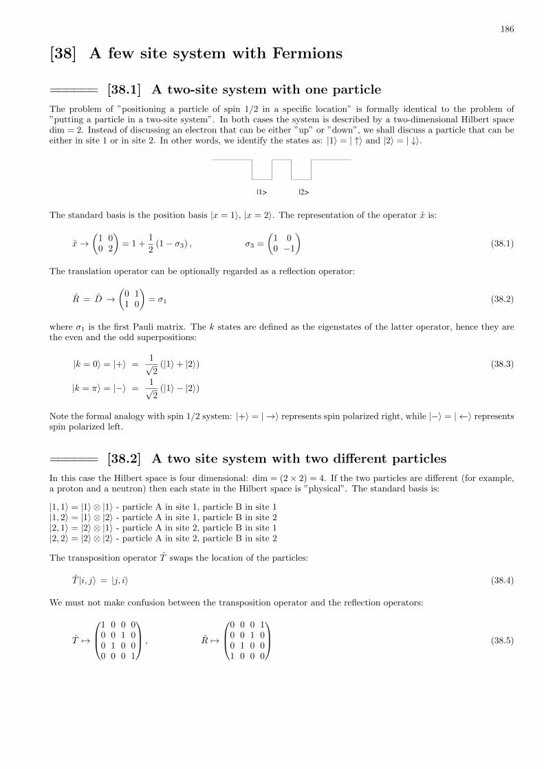
186

[38] A few site system with Fermions

====== [38.1] A two-site system with one particle

The problem of ”positioning a particle of spin 1/2 in a specific location” is formally identical to the problem of”putting a particle in a two-site system”. In both cases the system is described by a two-dimensional Hilbert spacedim = 2. Instead of discussing an electron that can be either ”up” or ”down”, we shall discuss a particle that can beeither in site 1 or in site 2. In other words, we identify the states as: |1〉 = | ↑〉 and |2〉 = | ↓〉.

|1> |2>

The standard basis is the position basis |x = 1〉, |x = 2〉. The representation of the operator x is:

x→(

1 00 2

)= 1 +

1

2(1− σ3) , σ3 =

(1 00 −1

)(38.1)

The translation operator can be optionally regarded as a reflection operator:

R = D →(

0 11 0

)= σ1 (38.2)

where σ1 is the first Pauli matrix. The k states are defined as the eigenstates of the latter operator, hence they arethe even and the odd superpositions:

|k = 0〉 = |+〉 =1√2

(|1〉+ |2〉) (38.3)

|k = π〉 = |−〉 =1√2

(|1〉 − |2〉)

Note the formal analogy with spin 1/2 system: |+〉 = | →〉 represents spin polarized right, while |−〉 = | ←〉 representsspin polarized left.

====== [38.2] A two site system with two different particles

In this case the Hilbert space is four dimensional: dim = (2× 2) = 4. If the two particles are different (for example,a proton and a neutron) then each state in the Hilbert space is ”physical”. The standard basis is:

|1, 1〉 = |1〉 ⊗ |1〉 - particle A in site 1, particle B in site 1|1, 2〉 = |1〉 ⊗ |2〉 - particle A in site 1, particle B in site 2|2, 1〉 = |2〉 ⊗ |1〉 - particle A in site 2, particle B in site 1|2, 2〉 = |2〉 ⊗ |2〉 - particle A in site 2, particle B in site 2

The transposition operator T swaps the location of the particles:

T |i, j〉 = |j, i〉 (38.4)

We must not make confusion between the transposition operator and the reflection operators:

T 7→

1 0 0 00 0 1 00 1 0 00 0 0 1

, R 7→

0 0 0 10 0 1 00 1 0 01 0 0 0

(38.5)

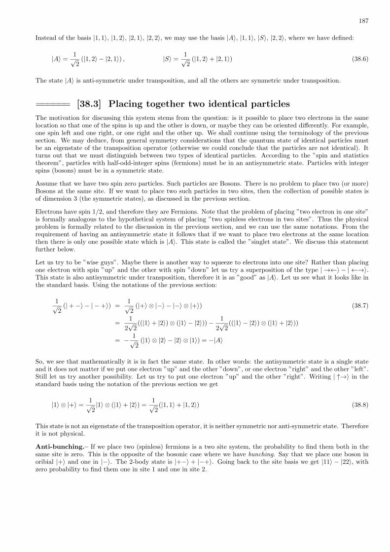
187

Instead of the basis |1, 1〉, |1, 2〉, |2, 1〉, |2, 2〉, we may use the basis |A〉, |1, 1〉, |S〉, |2, 2〉, where we have defined:

|A〉 =1√2

(|1, 2〉 − |2, 1〉) , |S〉 =1√2

(|1, 2〉+ |2, 1〉) (38.6)

The state |A〉 is anti-symmetric under transposition, and all the others are symmetric under transposition.

====== [38.3] Placing together two identical particles

The motivation for discussing this system stems from the question: is it possible to place two electrons in the samelocation so that one of the spins is up and the other is down, or maybe they can be oriented differently. For example,one spin left and one right, or one right and the other up. We shall continue using the terminology of the previoussection. We may deduce, from general symmetry considerations that the quantum state of identical particles mustbe an eigenstate of the transposition operator (otherwise we could conclude that the particles are not identical). Itturns out that we must distinguish between two types of identical particles. According to the ”spin and statisticstheorem”, particles with half-odd-integer spins (fermions) must be in an antisymmetric state. Particles with integerspins (bosons) must be in a symmetric state.

Assume that we have two spin zero particles. Such particles are Bosons. There is no problem to place two (or more)Bosons at the same site. If we want to place two such particles in two sites, then the collection of possible states isof dimension 3 (the symmetric states), as discussed in the previous section.

Electrons have spin 1/2, and therefore they are Fermions. Note that the problem of placing ”two electron in one site”is formally analogous to the hypothetical system of placing ”two spinless electrons in two sites”. Thus the physicalproblem is formally related to the discussion in the previous section, and we can use the same notations. From therequirement of having an antisymmetric state it follows that if we want to place two electrons at the same locationthen there is only one possible state which is |A〉. This state is called the ”singlet state”. We discuss this statementfurther below.

Let us try to be ”wise guys”. Maybe there is another way to squeeze to electrons into one site? Rather than placingone electron with spin ”up” and the other with spin ”down” let us try a superposition of the type | →←〉 − | ←→〉.This state is also antisymmetric under transposition, therefore it is as ”good” as |A〉. Let us see what it looks like inthe standard basis. Using the notations of the previous section:

1√2

(|+−〉 − | −+〉) =1√2

(|+〉 ⊗ |−〉 − |−〉 ⊗ |+〉) (38.7)

=1

2√

2((|1〉+ |2〉)⊗ (|1〉 − |2〉))− 1

2√

2((|1〉 − |2〉)⊗ (|1〉+ |2〉))

= − 1√2

(|1〉 ⊗ |2〉 − |2〉 ⊗ |1〉) = −|A〉

So, we see that mathematically it is in fact the same state. In other words: the antisymmetric state is a single stateand it does not matter if we put one electron ”up” and the other ”down”, or one electron ”right” and the other ”left”.Still let us try another possibility. Let us try to put one electron ”up” and the other ”right”. Writing | ↑→〉 in thestandard basis using the notation of the previous section we get

|1〉 ⊗ |+〉 =1√2|1〉 ⊗ (|1〉+ |2〉) =

1√2

(|1, 1〉+ |1, 2〉) (38.8)

This state is not an eigenstate of the transposition operator, it is neither symmetric nor anti-symmetric state. Thereforeit is not physical.

Anti-bunching.– If we place two (spinless) fermions is a two site system, the probability to find them both in thesame site is zero. This is the opposite of the bosonic case where we have bunching. Say that we place one boson inoribial |+〉 and one in |−〉. The 2-body state is |+−〉 + |−+〉. Going back to the site basis we get |11〉 − |22〉, withzero probability to find them one in site 1 and one in site 2.

188

[39] Boxes and NetworksA 1D segment can be regarded as the continuum limit of a discrete tight-binding chain. If the particle in confinedbetween two ends, the model is know as ”infinite well” or as ”1D box”. If there are periodic boundary conditions, themodel is know as ”1D ring”. Several ”1D boxes” can be connected into a network: each 1D segment is called ”bond”,and the junctions are called ”vortices”.

The ends of an isolated bond can be regarded as hard walls. It is easily argued that the wavefunction should satisfyDirichlet boundary conditions at the boundary of a hard wall. The perturbation which is created by an infinitesimaldisplacement of the wall is finite (see section below).

The coupling between two wavefunctions in a network due to the introduction of a connecting junction can be deducedby considering a wire which is divided by a high uδ(x) barrier (see section below).

We characterize a network by specifying the lengths La of the bonds, and the the potentials u at each vertex. Giventhis information we would like to find the eigenfunctions and the eigenenergies. We describe below two procedures forthat purpose: one is based on a straightforward generalization of the standard matching conditions, while the otheris based on the scattering matrix formalism.

====== [39.1] Hard walls

Let us assume that we have a particle in a one dimensional box of length L, such that V (x) = 0 within the interval0 < x < L. We assume Dirichlet boundary conditions at x = 0, while at x = L0 we assume a potential step, such thatV (x) = V0 for x > L0. We are going to see that if we take the limit V0 →∞, then this implies Dirichlet boundaryconditions at x = L0 too.

The wavefunction of nth eigenstate has to satisfy the Dirichlet boundary conditions at x = 0, and therefore has to beof the form

ψ(x) =

A sin(kx) for 0 < x < LBe−αx for x > L

(39.1)

where

k =√

2mE (39.2)

α =√

2m(V0 − E) ≈√

2mV0

The normalization factor at the limit V0 →∞ is A = (2/L)1/2. It would be convenient later to make the replacementA 7→ (−1)nA, in order to have the same sign for ψ(x) at x ∼ L. The matching condition at x = L is:

ψ‘(x)

ψ(x)

∣∣∣∣x=L−0

=ψ‘(x)

ψ(x)

∣∣∣∣x=L+0

= −α (39.3)

Consequently the eigenvalue equation is

k cot(kL) = −α (39.4)

In the limit V0 →∞ the equation becomes sin(kL) = 0 which implies that the unperturbed eigen-energies areEn = k2

n/2m with kn = (π/L)n. In this limit we see that the matching condition at x = L simply forces the wave-function to be zero there. Thus we have established that Hard walls implies Dirichlet boundary conditions.

Perturbation due to wall displacement.– We would like to find the perturbation due to a small shift dL in theposition of the wall. We keep V0 finite, but assume that it is very very large. We shall take the strict limit V0 → ∞only at the end of the calculation. For L = L0 the unperturbed Hamiltonian after digonalization is

[H0]nm =1

2m

(π

L0n

)2

δnm (39.5)

189

If we displace the wall a distance dL the new Hamiltonian becomes H = H0 + dLW . We ask what are the matrixelements Wnm of this perturbation. At first sight it looks as if to displace an ”infinite wall” constitutes ”infiniteperturbation” and hence Wnm =∞. But in fact it is not like that. We shall see that

Wnm = − π2

mL30

nm, [note sign convention] (39.6)

It is easily verified that the diagonal terms WnndL of the perturbation matrix give correctly the first order shift dEnof the energy levels due to the dL displacement.

Derivation.– The Hamiltonian of the unperturbed system, and the Hamiltonian after we have displaced the wall adistance dL are respectively

H0 =p2

2m+ V (x), H =

p2

2m+ V (x) (39.7)

The perturbation is:

δV (x) = V (x)− V (x) ≡ dL×W (39.8)

which is a rectangle of width dL and height −V0. It follows that the matrix elements of the perturbation are

Wnm =1

dL

∫ L+dL

L

ψ(n)(x)[−V0]ψ(m)(x)dx = −V0ψ(n)(L)ψ(m)(L) (39.9)

The ”matching conditions” allow to express ψ(0) using its derivative as −(1/α)ψ′(0), leading to

Wnm = − 1

2m

(d

dxψ(n)(L)

)(d

dxψ(m)(L)

)(39.10)

The last expression has only an implicit dependence on V0, through the derivatives of the wavefunctions at x = L.Obviously the limit V0 →∞ gives a well defined finite result:

d

dxψ(n)(x)

∣∣∣∣x=L

=

√2

Lkn =

[2π2

L3

]1/2

n (39.11)

leading to the result for Wnm that has been cited in the introduction to this derivation.

====== [39.2] The two-terminal delta junction

The simplest non-trivial example for an S matrix, is for a system which is composed of two 1D wires labeled as i = 1, 2,attached by a junction that is modeled as a delta barrier uδ(x). Using the standard ”s-scattering” convention thechannel wavefunctions are written as Ψ(r) ∝ Ai exp(−ikr)−Bi exp(ikr) where r = |x|. The linear relation betweenthe As and the Bs is determined by the matching conditions. The matching conditions for the channel wavefunctionat the origin r = 0 in the case of a delta barrier are further discussed in the next subsection, where it is also generalizedto the case of having a junction with M wires. The S matrix which is implied by these matching conditions is

S = −(r tt r

), [such that S=1 for u=∞] (39.12)

190

with

v ≡ (2E/m)1/2 (39.13)

t =1

1 + i(u/v)(39.14)

r = −1 + t (39.15)

There is a more elegant way to re-write this expression. Define the phase

γ ≡ phase(v + iu) ∈ [0, π/2] (39.16)

Then it follows that

|t|2 = (cos(γ))2 phase(t) = −γ (39.17)

|r|2 = (sin(γ))2 phase(r) = −γ − (π/2) (39.18)

In practice it is more convenient to use in the present context an ad-hoc convention of writing a raw-swapped Smatrix, corresponding to the re-definition of the outgoing amplitudes as B1 = −B2 and B2 = −B1, namely,

S =

(t rr t

)= e−iγ

( √geiφ −i

√1−ge−iα

−i√

1−geiα√ge−iφ

)[such that S=1 for u=0] (39.19)

with α = φ = 0 and

g = |t|2 =1

1 + (u/vE)2= (cos(γ))2 (39.20)

The advantage of the ad-hoc convention is the possibility to regard u = 0 as the unperturbed Hamiltonian, and touse the T matrix formalism to find the S matrix. All the elements of the T matrix equal to the same number T , andthe equality S = 1− iT implies that r = −iT and t = 1− iT .

====== [39.3] The multi-terminal delta junction

The simplest junction is composed ofM = 2 wires that are connected at one point. We can model such a junction asa delta barrier V (x) = uδ(x). The matching condition at x = 0 is implied by the Schrodinger equation, and relatesthe jump in the derivative to the value of the wavefuntion at that point.

1

2m[∂ψ(+0)− ∂ψ(−0)] = u ψ(0) (39.21)

A more elegant way of writing this relation is

M∑a=1

dψadr

∣∣∣∣r=0

= Mmuψ(0) (39.22)

with M = 2. The derivative of the radial functions ψ1(r) = ψ(−r) and ψ2(r) = ψ(+r) is with respect to the radialcoordinate r = |x|. It is implicit that these wavefuntions should have the same value at the meeting point r = 0. If wehaveM wires connected at one point we can define a generalized “delta junction” using the same matching condition.Say that we have a = 1, 2, 3 leads. The matching conditions at the junction are ψ1(0) = ψ2(0) = ψ3(0) ≡ ψ(0) while

191

the sum over the radial derivatives should equal Mmuψ(0). This means that the sum over the outgoing currents iszero.

More generally a junction can be fully characterized by its S matrix. So we can ask what is the S matrix of a deltajunction. It is straightforward to find out that the S matrix which is implied by the above matching conditions is

Sab = δab −2

M

(1

1 + i(u/vE)

)[such that S=1 for u=∞] (39.23)

For u = 0 we get zero reflection if M = 2, while if M = 3 we get

S =

+1/3 −2/3 −2/3−2/3 +1/3 −2/3−2/3 −2/3 +1/3

(39.24)

In the limit M→∞ we get total reflection.

Sometimes we want to treat the connecting junction as a perturbation. Consider for example the simplest possibilityof having two 1D boxes connected at x = 0 hence forming a double well structure which is described by a HamiltonianH(x, p;u) in which the barrier is represented by V (x) = uδ(x). The eigenstates n of the unperturbed HamiltonianH(x, p;∞) are those of the left box together with those of the right box. We want to have an explicit expressionfor the perturbation Wnm due to the coupling at x = 0. Note that W is defined as the difference H(u)−H(∞) soit is not the same as V = H(u)−H(0). We can obtain the total perturbation W from a sequence of infinitesimalvariations of the barrier height starting from u =∞. Namely,

H(u) = H(∞)−∫ ∞u

(∂H∂u

)du′ ≡ H(∞) +W (39.25)

For any value of u the Hilbert space of the system is spanned by a set of (real) eigenfunction labeled by n. The matrixelements for an infinitesimal variation of the barrier height is

(∂H∂u

)nm

= ψ(n)(0) ψ(m)(0) =1

(2mu)2

[dψ(n)

dr

]0

[dψ(m)

dr

]0

(39.26)

where is the last step we have used the matching conditions in order to express the wave function by the total radialderivative. As long as the barrier has small transmission (g 1), the nth and the mth states remain similar to theunperturbed states and accordingly, upon integration, we get the result [arXiv:0807.2572]

Wnm = − 1

4m2u

[dψ(n)

dr

]0

[dψ(m)

dr

]0

(39.27)

The d/dr in this expression is the total radial derivative, but in fact the contribution comes from one term only,because the unperturbed wavefunction of a given eigenstate ψ(n) is non-zero only in one box.

====== [39.4] Finding the eigenstates of a network

Consider a network which is composed of b bonds and v vertexes. The wavefunction on bond a ≡ (i, j) that connectsvertex i to vertex j is written as

ψa(x) = Baeikax +Aae−ikax (39.28)

where 0 < x < La is the position of the particle along the bond with the origin at vertex i. Note that the wavefunctionon a = (j, i) is with Aa = BaeikaLa and Ba = Aae−ikaLa . The wavenumber is ka =

√2mE + (φa/La), where φa is

192

determined by the vector potential. Note that φa = −φa. For simplicity we assume below that there is no magneticfield, and accordingly ka = ka.

The most economical way to represent the wavefunction is by a vector ψ 7→ ψ1, ψ2, ..., ψv that contains the waveamplitudes at the vertexes. If we know this vector then we can construct the whole wavefunction on bond a = (i, j)using the formula

ψa(x) =1

sin(kaLa)

[ψi sin(ka(La−x)) + ψj sin(kax)

](39.29)

The in order to find the eigenstates we simply have to write the v matching conditions of the vertexes, and look forthe energies E for which there is non-trivial solution for this homogeneous set of equations.

Optionally the wavefunction can be represented by the vector A = Aa of length 2b, or equivalently by the vectorB = Ba. The wavefunction and its gradient in a particular vertex are related to the latter as follows:

ψ = B +A (39.30)

∂ψ = ik × (B −A) (39.31)

If the junctions are represented by a scattering matrix and not by a simple matching condition there is an optionalprocedure for finding the eigenstates. The A and the B vectors are related by

B = S A (39.32)

A = J eikL B (39.33)

where S is a 2b × 2b matrix that relates the outgoing to the ingoing fluxes, and J is a 2b × 2b permutation matrixthat induces the mapping a 7→ a, and L = diagLa, and k = diagka. The equation for the eigenstates is

(JeikLS − 1

)A = 0 (39.34)

We can get from this equation a set of eigenvalues En with the corresponding eigenvectors A(n) and the associatedamplitudes B(n) = SA(n).

The S matrix of the network (if appropriately ordered) has a block structure, and can be written as S =∑j S

j ,

where Sj is the vj×vj block that describes the scattering in the jth vertex. vj is the number of leads that stretch outof that vertex. A delta function scatterer is regarded as a vj = 2 vertex. Let us construct a simple example. Considera ring with two delta barriers. Such ring can be regarded as a network with two bonds. The bonds are labeled as12, 12′, 21, 21′, where the prime distinguishes the second arm. The matrices that define the system are

S =

r1 t1 0 0t1 r1 0 00 0 r2 t20 0 t2 r2

, L =

L 0 0 00 L′ 0 00 0 L 00 0 0 L′

, J =

0 0 1 00 0 0 11 0 0 00 1 0 0

(39.35)

Finally we note that k =√

2mE + φ/L, where the fluxes matrix is φ = diagφa. If there is a single flux line φ onecan write φ = φP , where P can be expressed as a linear combination of the channel projectors Pa. For example, ifonly one wire a encloses the flux line, then P = Pa − Pa and we get

k =1

~√

2mE + φP

L(39.36)

The obvious application of this procedure is for the analysis of a multi-mode Aharonov-Bohm ring, where the ”bonds”are the propagation-modes of the ring, and they all enclose the same flux line.

193

QM in Practice (part II)

[40] Approximation methods for finding eigenstates

====== [40.1] The WKB approximation

In the next sections we discuss the canonical version of perturbation theory. The small parameter is the strengthof the perturbation. Another family of methods to find approximate expressions for the eigen-functions is based ontreating “~” as the small parameter. The ~ in this context is not the ~ of Planck but rather its scaled dimensionlessversion that controls quantum-to-classical correspondence. For a particle in a box the scaled ~ is the ratio between theDe-Broglie wavelength and the linear size of the box. Such approximation methods are known as semi-classical. Themost elementary example is known as the WKB (Wentzel, Kramers, Brillouin) approximation [Messiah p.231]. It isdesigned to treat slowly varying potentials in 1D where the wavefunction looks locally like a plane wave (if V (x) < E)or as a decaying exponential (in regions where V (x) > E). The refined version of WKB, which is known as ”uniformapproximation”, allows also to do the matching at the turning points (where V (x) ∼ E). The generalization of thed = 1 WKB for d > 1 dimensions integrable systems is known as the EBK scheme. There is also a different type ofgeneralization for d > 1 chaotic systems, via the Wigner Weyl formalism.

Assuming free wave propagation, hence neglecting back reflection, the WKB wavefunction is written as

Ψ(x) =√ρ(x)eiS(x) (40.1)

This expression is inserted into the 1D Schrodinger equation. In leading order in ~ we get a continuity equation forthe probability density ρ(x), while the local wavenumber should be as expected

dS(x)

dx= p(x) =

√2m(E − V (x)) (40.2)

Hence (for a right moving wave) one obtains the WKB approximation

ψ(x) =1√p(x)

EXP[i

∫ x

x0

p(x′)dx′]

(40.3)

where x0 is an arbitrary point. For a standing wave the ”EXP” can be replaced by either ”sin” or ”cos”. It shouldbe clear that for a ”flat” potential floor this expression becomes exact. Similarly in the ”forbidden” region we have adecaying exponential. Namely, the local wavenumber ±p(x) is replaced by ±iα(x), where α(x) = (2m(V (x)−E))1/2.

Scattering.– If we have a scattering problem in one dimension we can use the WKB expression (with exp) in order todescribe (say) a right moving wave. It should be realized that there is no back-reflection within the WKB framework,but still we can calculate the phase shift for the forward scattering:

θWKB =

∫ ∞−∞

p(x)dx−∫ ∞−∞

pEdx =

∫ ∞−∞

[√2m(E − V (x))−

√2mE

]dx (40.4)

=√

2mE

∫ ∞−∞

[√1− V (x)

E− 1

]dx ≈ −

√m

2E

∫ ∞−∞

V (x)dx

Hence we get

θWKB = − 1

~vE

∫ ∞−∞

V (x)dx (40.5)

194

It should be noted that θWKB1D is the phase shift in a 1D scattering geometry (−∞ < x <∞). A similar looking result

for semi-1D geometry (r > 0) is known as the Born approximation for the phase shift.

Bound states.– If we have a particle in a well, then there are two turning points x1 and x2. On the outer sides of thewell we have WKB decaying exponentials, while in the middle we have a WKB standing wave. As mentioned abovethe WKB scheme can be extended so as to provide matching conditions at the two turning points. Both matchingconditions can be satisfied simultaneously if

∫ x2

x1

p(x)dx =

(1

2+ n

)π~ (40.6)

where n = 0, 1, 2, . . . is an integer. Apart from the 1/2 this is a straightforward generalization of the quantizationcondition of the wavenumber of a particle in a 1D box with hard walls (k × (x2 − x1) = nπ). The (1/2)π phase shiftarise because we assume soft rather than hard walls. This 1/2 becomes exact in the case of harmonic oscillator.

The WKB quantization condition has an obvious phase space representation, and it coincides with the ”Born Oppen-heimer quantization condition”:

∮p(x)dx =

(1

2+ n

)2π~ (40.7)

The integral is taken along the energy contour which is formed by the curves p = ±p(x). This expression implies thatthe number of states up to energy E is

N (E) =x

H(x,p)<E

dxdp

2π~(40.8)

The d > 1 generalization of this idea is the statement that the number of states up to energy E is equal to the phasespace volume divided by (2π~)d. The latter statement is known as Weyl law, and best derived using the Wigner-Weylformalism.

====== [40.2] The variational scheme

The variational scheme is an approximation method that is frequently used either as an alternative or in combinationwith perturbation theory. It is an extremely powerful method for the purpose of finding the ground-state. Moregenerally we can use it to find the lowest energy state within a subspace of states.

The variational scheme is based on the trivial observation that the ground state minimize the energy functional

F [ψ] ≡ 〈ψ|H|ψ〉 (40.9)

If we consider in the variational scheme the most general ψ we simply recover the equation Hψ = Eψ and hencegain nothing. But in practice we can substitute into F [] a trial function ψ that depends on a set of parametersX = (X1, X2, ...). Then we minimize the function F (X) = F [ψ] with respect to X.

The simplest example is to find the ground state on an harmonic oscillator. If we take the trail function as a Gaussianof width σ, then the minimization of the energy functional with respect to σ will give the exact ground state. If weconsider an anharmonic oscillator we still can get a very good approximation. A less trivial example is to find bondingorbitals in a molecules using as a trial function a combination of hydrogen-like orbitals.

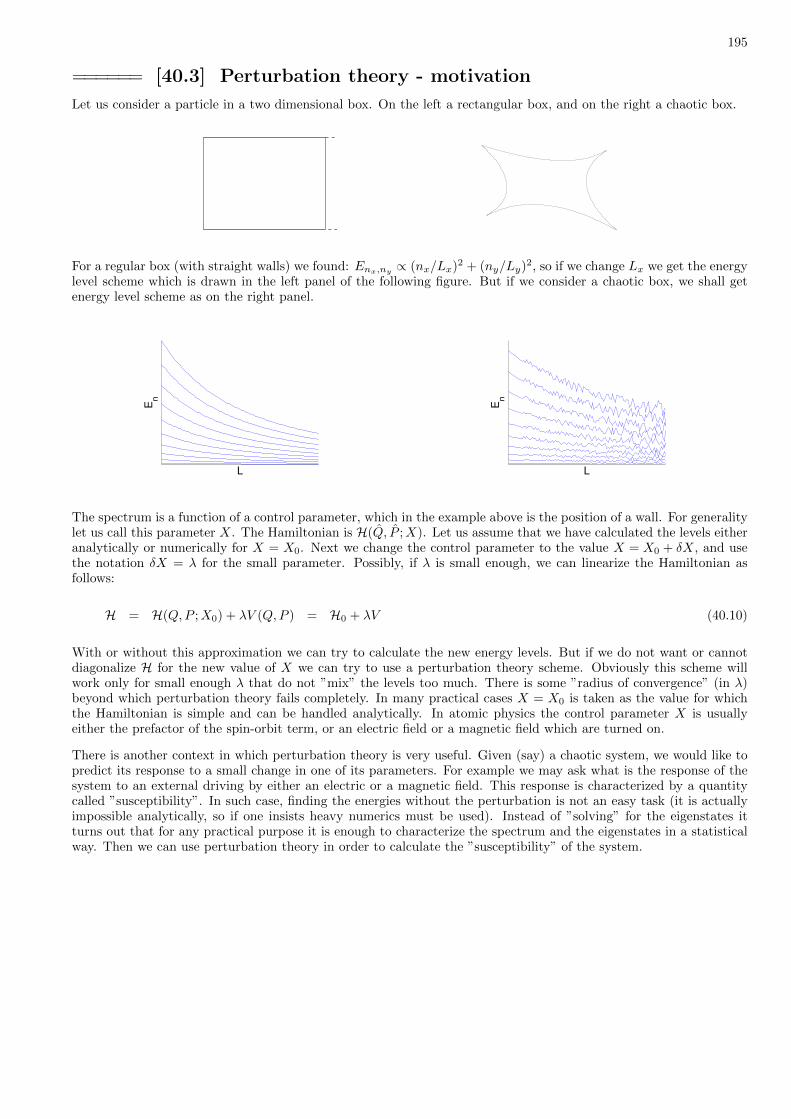
195

====== [40.3] Perturbation theory - motivation

Let us consider a particle in a two dimensional box. On the left a rectangular box, and on the right a chaotic box.

For a regular box (with straight walls) we found: Enx,ny ∝ (nx/Lx)2 + (ny/Ly)2, so if we change Lx we get the energylevel scheme which is drawn in the left panel of the following figure. But if we consider a chaotic box, we shall getenergy level scheme as on the right panel.

L

E n

L

E n

The spectrum is a function of a control parameter, which in the example above is the position of a wall. For generalitylet us call this parameter X. The Hamiltonian is H(Q, P ;X). Let us assume that we have calculated the levels eitheranalytically or numerically for X = X0. Next we change the control parameter to the value X = X0 + δX, and usethe notation δX = λ for the small parameter. Possibly, if λ is small enough, we can linearize the Hamiltonian asfollows:

H = H(Q,P ;X0) + λV (Q,P ) = H0 + λV (40.10)

With or without this approximation we can try to calculate the new energy levels. But if we do not want or cannotdiagonalize H for the new value of X we can try to use a perturbation theory scheme. Obviously this scheme willwork only for small enough λ that do not ”mix” the levels too much. There is some ”radius of convergence” (in λ)beyond which perturbation theory fails completely. In many practical cases X = X0 is taken as the value for whichthe Hamiltonian is simple and can be handled analytically. In atomic physics the control parameter X is usuallyeither the prefactor of the spin-orbit term, or an electric field or a magnetic field which are turned on.

There is another context in which perturbation theory is very useful. Given (say) a chaotic system, we would like topredict its response to a small change in one of its parameters. For example we may ask what is the response of thesystem to an external driving by either an electric or a magnetic field. This response is characterized by a quantitycalled ”susceptibility”. In such case, finding the energies without the perturbation is not an easy task (it is actuallyimpossible analytically, so if one insists heavy numerics must be used). Instead of ”solving” for the eigenstates itturns out that for any practical purpose it is enough to characterize the spectrum and the eigenstates in a statisticalway. Then we can use perturbation theory in order to calculate the ”susceptibility” of the system.

196

====== [40.4] Perturbation theory - a mathematical digression

Let us illustrate how the procedure of perturbation theory is applied in order to find the roots of a toy equation.Later we shall apply the same procedure to find the eigenvalues and the eigenstates of a given Hamiltonian. The toyequation that we consider is

x+ λx5 = 3 (40.11)

We assume that the magnitude of the perturbation (λ) is small. The Taylor expansion of x with respect to λ is:

x(λ) = x(0) + x(1)λ+ x(2)λ2 + x(3)λ3 + . . . (40.12)

The zero-order solution gives us the solution for the case λ = 0:

x(0) = 3 (40.13)

To find the perturbed solution substitute the expansion:

[x(0) + x(1)λ+ x(2)λ2 + ...

]+ λ

[x(0) + x(1)λ+ x(2)λ2 + ...

]5= 3 (40.14)

This can be re-arranged as follows:

[x(0) − 3

]+[x(1) + (x(0))5

]λ +

[5(x(0))4x(1) + x(2)

]λ2 + O(λ3) = 0 (40.15)

By comparing coefficients we get a system of equations that can be solved iteratively order by order:

x(0) = 3 (40.16)

x(1) = −(x(0))5 = −35 (40.17)

x(2) = −5(x(0))4x(1) = 5× 39 (40.18)

It is obviously possible to find the corrections for higher orders by continuing in the same way.

197

[41] Perturbation theory for the eigenstates

====== [41.1] Degenerate perturbation theory (zero-order)

Consider a diagonal Hamiltonian matrix, with a small added perturbation that spoils the diagonalization:

H =

2 0.03 0 0 0 0.5 00.03 2 0 0 0 0 0

0 0 2 0.1 0.4 0 00 0 0.1 5 0 0.02 00 0 0.4 0 6 0 0

0.5 0 0 0.02 0 8 0.30 0 0 0 0 0.3 9

(41.1)

The Hamiltonian can be visualized using an energy level diagram:

2

89

65

The eigenvectors without the perturbation are:

1000000

0100000

0010000

· · · (41.2)

The perturbation spoils the diagonalization. The question we would like to answer is what are the new eigenvaluesand eigenstates of the Hamiltonian. We would like to find them ”approximately”, without having to diagonalize theHamiltonian again. First we will take care of the degenerated blocks. The perturbation can remove the existingdegeneracy. In the above example we make the following diagonalization:

2 ·

1 0 00 1 00 0 1

+ 0.03 ·

0 1 01 0 00 0 0

→

1.97 0 00 2.03 00 0 2

(41.3)

We see that the perturbation has removed the degeneracy. At this stage our achievement is that there are no matrixelements that couple degenerate states. This is essential for the next steps: we want to ensure that the perturbativecalculation would not diverge.

198

For the next stage we have to transform the Hamiltonian to the new basis. See the calculation in the Mathematicafile ”diagonalize.nb”. If we diagonalize numerically the new matrix we find that the eigenvector that corresponds tothe eigenvalue E ≈ 5.003 is

|Ψ〉 →

0.00080.03

0.00081

−0.01−0.0070.0005

=

0001000

+

0.00080.03

0.00080

−0.01−0.0070.0005

≡ Ψ[0]

n + Ψ[1,2,3,... ]n (41.4)

We note that within the scheme of perturbation theory it is convenient to normalize the eigenvectors according to thezero order approximation. We also use the convention that all the higher order corrections have zero overlap with thezero order solution. Else the scheme of the solution becomes ill defined.

====== [41.2] Perturbation theory to arbitrary order

We write the Hamiltonian as H = H0 + λV where V is the perturbation and λ is the control parameter. Note thatλ can be ”swallowed” in V . We keep it during the derivation in order to have clear indication for the ”order” of theterms in the expansion. The Hamiltonian is represented in the unperturbed basis as follows:

H = H0 + λV =∑n

|n〉εn〈n| + λ∑n,m

|n〉Vn,m〈m| (41.5)

which means

H →

ε1 0 0 00 ε2 0 00 0 ε3 00 0 0 . . .

+ λ

V1,1 V1,2 . . . . . .V2,1 V2,2 . . . . . .. . . . . . . . . . . .. . . . . . . . . . . .

(41.6)

In fact we can assume without loss of generality that Vn,m = 0 for n = m, because these terms can be swallowed intothe diagonal part. Most importantly we assume that none of the matrix element couples degenerated states. Suchcouplings should be treated in the preliminary ”zero order” step that has been discussed in the previous section.

We would like to introduce a perturbative scheme for finding the eigenvalues and the eigenstates of the equation

(H0 + λV )|Ψ〉 = E|Ψ〉 (41.7)

The eigenvalues and the eigenvectors are expanded as follows:

E = E[0] + λE[1] + λ2E[2] + · · · (41.8)

Ψn = Ψ[0]n + λΨ[1]

n + λ2Ψ[2]n

where it is implicit that the zero order solution and the normalization are such that

E[0] = εn0(41.9)

Ψ[0]n = δn,n0

Ψ[1,2,3,... ]n = 0 for n = n0

It might be more illuminating to rewrite the expansion of the eigenvector using Dirac notations. For this purpose welabel the unperturbed eigenstates as |εn〉 and the perturbed eigenstates as |En〉. Then the expansion of the latter is

199

written as

|En0〉 = |E[0]

n0〉+ λ|E[1]

n0〉+ λ2|E[2]

n0〉+ · · · (41.10)

hence

〈εn|En0〉 = δn,n0

+ λ〈εn|E[1]n0〉+ λ2〈εn|E[2]

n0〉+ · · · (41.11)

which coincides with the traditional notation. In the next section we introduce a derivation that leads to the followingpractical results (absorbing λ into the definition of V ):

Ψ[0]n = δn,n0 (41.12)

Ψ[1]n =

Vn,n0

εn0− εn

E[0] = εn0

E[1] = Vn0,n0

E[2] =∑

m(6=n0)

Vn0,mVm,n0

εn0 − εm

The calculation can be illustrated graphically using a ”Feynman diagram”. For the calculation of the second ordercorrection to the energy we should sum all the paths that begin with the state n0 and also end with the state n0.We see that the influence of the nearer levels is much greater than the far ones. This clarifies why we cared to treatthe couplings between degenerated levels in the zero order stage of the calculation. The closer the level the strongerthe influence. This influence is described as ”level repulsion”. Note that in the absence of first order correction theground state level always shifts down.

====== [41.3] Derivation of the results

The equation we would like to solve is

ε1 0 0 00 ε2 0 00 0 ε3 00 0 0 . . .

Ψ1

Ψ2

. . .

+ λ

V1,1 V1,2 . . . . . .V2,1 . . . . . . . . .. . . . . . . . . . . .. . . . . . . . . . . .

Ψ1

Ψ2

. . .

= E

Ψ1

Ψ2

. . .

(41.13)

Or, in index notation:

εnΨn + λ∑m

Vn,mΨm = EΨn (41.14)

This can be rewritten as

(E − εn)Ψn = λ∑m

Vn,mΨm (41.15)

We substitute the Taylor expansion:

E =∑k=0

λkE[k] = E[0] + λE[1] + . . . (41.16)

Ψn =∑k=0

λkΨ[k]n = Ψ[0]

n + λΨ[1]n + . . .

200

We recall that E[0] = εn0 , and

Ψ(0)n = δn,n0

→

. . .00100. . .

, Ψ[k 6=0]

n →

. . .??0??. . .

(41.17)

After substitution of the expansion we use on the left side the identity

(a0 + λa1 + λ2a2 + . . . )(b0 + λb1 + λ2b2 + . . . ) =∑k

λkk∑

k′=0

ak′bk−k′ (41.18)

Comparing the coefficients of λk we get a system of equations k = 1, 2, 3...

k∑k′=0

E[k′]Ψ[k−k′]n − εnΨ[k]

n =∑m

Vn,mΨ[k−1]m (41.19)

We write the kth equation in a more expanded way:

(E[0] − εn)Ψ(k)n + E[1]Ψ[k−1]

n + E[2]Ψ[k−2]n + · · ·+ E[k]Ψ[0]

n =∑m

Vn,mΨ[k−1]m (41.20)

If we substitute n = n0 in this equation we get:

0 + 0 + · · ·+ E[k] =∑m

Vn0,mΨ[k−1]m (41.21)

If we substitute n 6= n0 in this equation we get:

(εn0− εn)Ψ[k]

n =∑m

Vn,mΨ[k−1]m −

k−1∑k′=1

E[k′]Ψ[k−k′]n (41.22)

Now we see that we can solve the system of equations that we got in the following order:

Ψ[0] → E[1] , Ψ[1] → E[2] , Ψ[2] → E[3] , Ψ[3] → . . . (41.23)

where:

E[k] =∑m

Vn0,mΨ[k−1]m (41.24)

Ψ[k]n =

1

(εn0 − εn)

[∑m

Vn,mΨ[k−1]m −

k−1∑k′=1

E[k′]Ψ[k−k′]n

]

The practical results that were cited in the previous sections are easily obtained from this iteration scheme.

201

====== [41.4] Delta scatterer in a box

Possibly the simplest non-trivial example for the demonstration of perturbation theory and its limitations is to findthe effect of introducing a delta scatterer V (r) = δ(r) in a box. We consider first the exact solution in the onedimensional (d = 1) case, where the delta is placed in the centre of segment |r| < R, and the d = 3 case, where thedelta is placed in the centre of sphere |r| < R. Later we consider the case of a delta in the centre of a rectangular box[−R,R]d. Below we use units such that the mass is unity, and also R = 1.

In the one dimensional case the wavefunction has to satisfy Dirichlet boundary conditions at the walls, and thematching condition across the delta barrier at the origin, leading to the eigenvalue equation k cot(k) = u for E > 0

and k coth(k) = u for E < 0 where k =√

2E. One observes that for u < −1 the ground state become bounded(E0 < 0), while all the other states are extended (with E > 0). For very negative u we get E0 ≈ −u2/2 andEn,− = (πn)2/2 and En,+ ≈ En,− that are slightly shifted downwards.

For d ≥ 2 the effect of introducing a delta scatterer is zero. This is complementary to the statement that a deltafunction has zero scattering cross-section. In order to have a non-zero effect the scatterer should have a finite size.To clarify the ”zero” effect of a point scatterer let us consider the eigenfunctions of a d = 3 sphere that has an infinitebarrier V0 of radius a in its centre. The zero angular momentum wavefuntions in the extreme case of an infinitebarrier are

Ψ(r, θ, ϕ) = constsin(k|r − a|)

r(41.25)

The healing length is of order a and in the limit a → 0 the “hole” in the wavefunction disappears irrespective ofwhether V0a

3 is kept constant or becomes infinite.

Now we would like to see how/whether the above results can be obtained formally via perturbation theory. For thispurpose it is most convenient to consider a delta function in a centre of a rectangular box (segment if d = 1, squareif d = 2). Excluding all the states that have node at the centre the Hamiltonian matrix takes the following form:

H =

ε1 0 0 0 ...0 ε2 0 0 ...0 0 ε3 0 ...0 0 0 ε4 ...... ... ... ... ...

+ u

1 1 1 1 ...1 1 1 1 ...1 1 1 1 ...1 1 1 1 ...... ... ... ... ...

(41.26)

We note that the same Hamiltonian (with u < 0) emerges in the analysis of the Copper pair problem, which has inspiredthe BCS theory of superconductivity. In turns out (see below) that the important information for the analysis is thedensity of states % ∝ εα, where α = (d/2)−1 with d = 1, 2, 3. If we introduce a cutoff and consider the finite-sizeHamiltonian that consists of the levels εn < ωc, it is like to give the scatterer a finite width a ∼ (2mωc)

−1/2.

The ground state energy using second order perturbation is

E0 = ε1 + u+∑n

u2

E0 − εn∼ −

∑n

u2

En(41.27)

In the one dimensional case this expression is finite and give a meaningful result if u 1. But if α ≥ 1 this sumdiverges in the ωc →∞ limit:

E0 ∼ −∑n

u2

En∼ −∞ (41.28)

This divergence obviously applies to all the levels, and to all orders of perturbation theory (we consider above theground state just as an example). It turns out from the exact analysis (below) that the this divergence indicatesthat the perturbation in an infinite order (exact) calculation has a zero effect. One way to think about this puzzlingobservation is to realize that the geometric sum 1 + x+ x2 + x3 + ... is formally zero (and not infinite) in the limitx→∞ because it equals 1/(1− x).

202

The exact solution of the eigenvalue problem requires to solve the matrix equation HΨ = EΨ, namely

εnΨn − u∑m

Ψm = EΨn (41.29)

Introduction the notation C =∑m Ψm, which later will be determined via normalization, we can solve for the

wavefunction:

Ψn = Cu

E − εn(41.30)

From the definition of C it follows that the eigenvalues should be the solution of the following equation:

∑ u

E − εn= 1 (41.31)

The equation has a nice graphical visualization, and one can easily be convinced that in the limit ωc → ∞ theperturbed eigenvalues approach the unperturbed values.

In view of the interest in the Cooper pair problem it is of interest to see what happens if we have constant density ofstates % with finite cutoff ωc and negative u. The graphical visualization implies that the ground state separates fromthe quasi-continuum and forms a bound state of energy E0 = −∆, as in the familiar d = 1 case. In order to estimate∆ we approximate the sum by an integral and get the equation

|u|% ln

(∆ + ωc

∆

)= 1 (41.32)

leading to

∆ =ωc

exp(

1|u|%

)− 1

(41.33)

In the limit of small u we have the BCS-like result ∆ = exp(−1/(|u|%)), while in the other extreme of very strongu we get ∆ = Nu where N = %ωc is the number of levels in the quasi-degenerated band. The latter result is easilyverified by direct diagonalization of of the Hamiltonian. Namely, if the unperturbed energies were degenerated theHamiltonian would become diagonal in the “momentum” representation, where only the zero momentum state isaffected.

203

[42] Perturbation theory / Wigner

====== [42.1] The overlap between the old and the new states

We have found that the perturbed eigenstates to first-order are given by the expression

|En〉 ≈ |εn〉+∑m

Vm,nεn − εm

|εm〉 (42.1)

So, it is possible to write:

〈εm|En〉 ≈Vmn

εn − εmfor m 6= n (42.2)

which implies

P (m|n) ≡ |〈εm|En〉|2 ≈ |Vmn|2

(Em − En)2for m 6= n (42.3)

In the latter expression we have replaced in the denominator the unperturbed energies by the perturbed energies.This is OK in leading order treatment. The validity condition is

|V | ∆ (42.4)

In other words, the perturbation must be much smaller than the mean level spacing. We observe that once thiscondition breaks down the sum

∑m P (m|n) becomes much larger than one, whereas the exact value should have unit

normalization. This means that if |V | ∆ the above first order expression cannot be trusted.

Can we do better? In principle we have to go to higher orders of perturbation theory, which might be very complicated.But in fact the generic result that comes out is quite simple:

P (m|n) ≈ |Vm,n|2

(Em − En)2 + (Γ/2)2(42.5)

This is called ”Wigner Lorentzian”. As we shall see later it is related to an exponential decay law that is called”Wigner decay”. The expression for the ”width” of this Lorentzian is implied by normalization:

Γ =2π

∆|V |2 (42.6)

The Lorentzian expression is not exact. It is implicit that we assume a dense spectrum (high density of states). Wealso assume that all the matrix elements are of the same order of magnitude. Such assumption can be justified e.g.in the case of a chaotic system. In order to show that

∑m P (m|n) =

∑n P (m|n) = 1 one use the recipe:

∑n

f(En) ≈∫dE

∆f(E) (42.7)

where ∆ is the mean level spacing. In the following we shall discuss further the notion Density of States (DOS) andLocal Density of States (LDOS) which are helpful in further clarifying the significance of the Wigner Lorentzian.

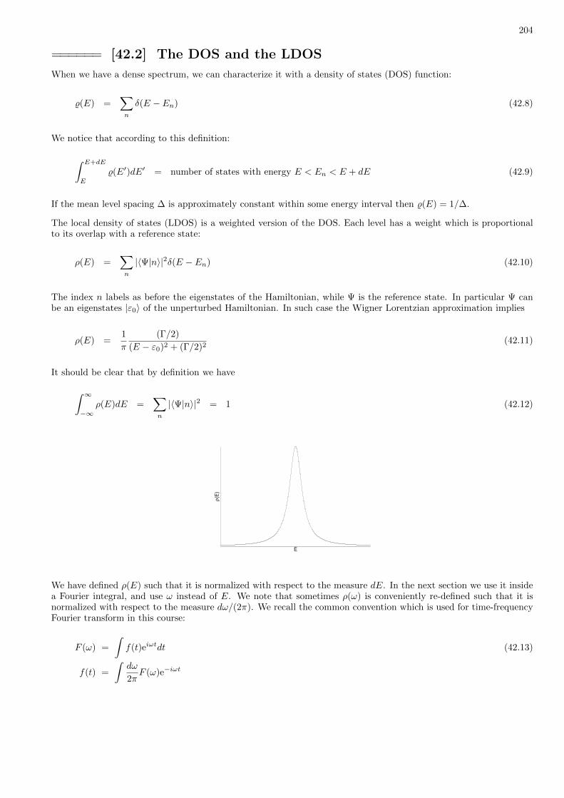
204

====== [42.2] The DOS and the LDOS

When we have a dense spectrum, we can characterize it with a density of states (DOS) function:

%(E) =∑n

δ(E − En) (42.8)

We notice that according to this definition:

∫ E+dE

E

%(E′)dE′ = number of states with energy E < En < E + dE (42.9)

If the mean level spacing ∆ is approximately constant within some energy interval then %(E) = 1/∆.

The local density of states (LDOS) is a weighted version of the DOS. Each level has a weight which is proportionalto its overlap with a reference state:

ρ(E) =∑n

|〈Ψ|n〉|2δ(E − En) (42.10)

The index n labels as before the eigenstates of the Hamiltonian, while Ψ is the reference state. In particular Ψ canbe an eigenstates |ε0〉 of the unperturbed Hamiltonian. In such case the Wigner Lorentzian approximation implies

ρ(E) =1

π

(Γ/2)

(E − ε0)2 + (Γ/2)2(42.11)

It should be clear that by definition we have

∫ ∞−∞

ρ(E)dE =∑n

|〈Ψ|n〉|2 = 1 (42.12)

E

ρ(E)

We have defined ρ(E) such that it is normalized with respect to the measure dE. In the next section we use it insidea Fourier integral, and use ω instead of E. We note that sometimes ρ(ω) is conveniently re-defined such that it isnormalized with respect to the measure dω/(2π). We recall the common convention which is used for time-frequencyFourier transform in this course:

F (ω) =

∫f(t)eiωtdt (42.13)

f(t) =

∫dω

2πF (ω)e−iωt

205

====== [42.3] Wigner decay and its connection to the LDOS

Let us assume that we have a system with many energy states. We prepare the system in the state |Ψ〉. Now weapply a field for a certain amount of time, and then turn it off. What is the probability P (t) that the system willremain in the same state? This probability is called the survival probability. By definition:

P (t) = |〈Ψ(0)|Ψ(t)〉|2 (42.14)

Let H0 be the unperturbed Hamiltonian, while H is the perturbed Hamiltonian (while the field is ”on”). In whatfollows the index n labels the eigenstates of the perturbed Hamiltonian H. We would like to calculate the survivalamplitude:

〈Ψ(0)|Ψ(t)〉 = 〈Ψ|U(t)|Ψ〉 =∑n

〈n|Ψ〉|2e−iEnt (42.15)

We notice that:

〈Ψ(0)|Ψ(t)〉 = FT

[∑n

〈n|Ψ〉|22πδ(ω − En)

]= FT [2πρ(ω)] (42.16)

If we assume that the LDOS is given by Wigner Lorentzian then:

P (t) =∣∣∣FT [2πρ(E)]

∣∣∣2 = e−Γt (42.17)

The Wigner decay appears when we ”break” first-order perturbation theory. The perturbation should be strongenough to create transitions to other levels. Else the system stays essentially at the same level all the time (P (t) ≈ 1).

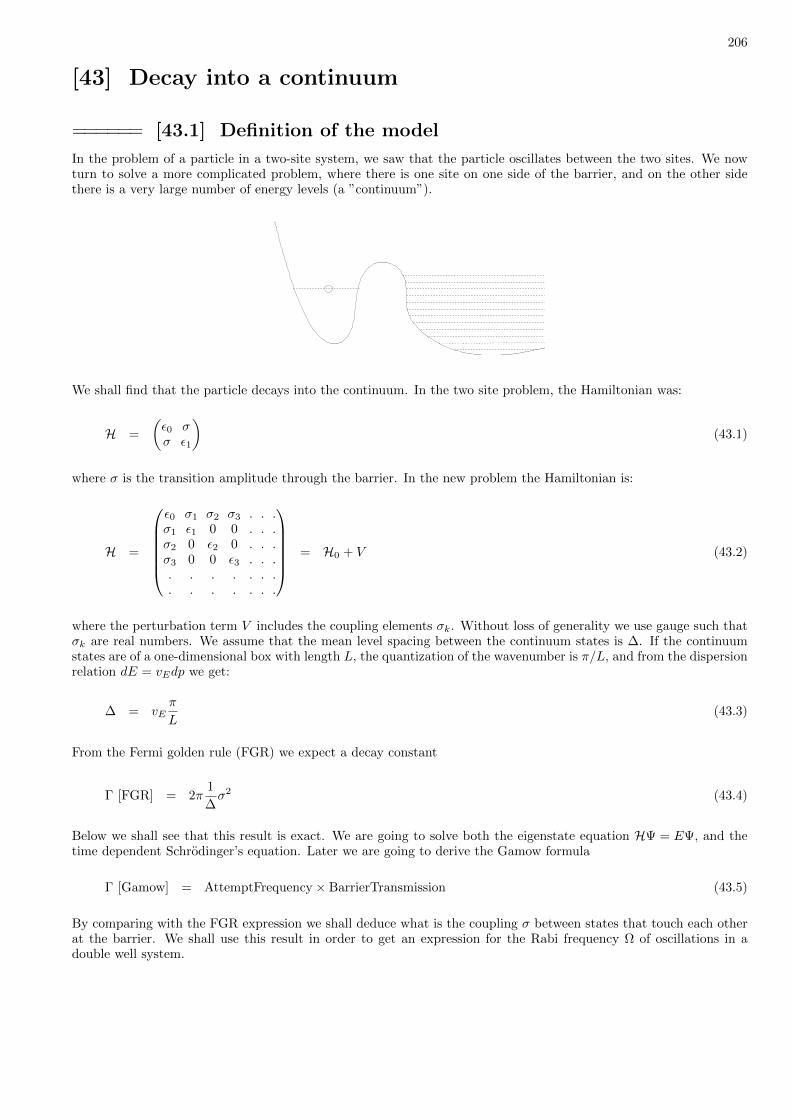
206

[43] Decay into a continuum

====== [43.1] Definition of the model

In the problem of a particle in a two-site system, we saw that the particle oscillates between the two sites. We nowturn to solve a more complicated problem, where there is one site on one side of the barrier, and on the other sidethere is a very large number of energy levels (a ”continuum”).

We shall find that the particle decays into the continuum. In the two site problem, the Hamiltonian was:

H =

(ε0 σσ ε1

)(43.1)

where σ is the transition amplitude through the barrier. In the new problem the Hamiltonian is:

H =

ε0 σ1 σ2 σ3 . . .σ1 ε1 0 0 . . .σ2 0 ε2 0 . . .σ3 0 0 ε3 . . .. . . . . . .. . . . . . .

= H0 + V (43.2)

where the perturbation term V includes the coupling elements σk. Without loss of generality we use gauge such thatσk are real numbers. We assume that the mean level spacing between the continuum states is ∆. If the continuumstates are of a one-dimensional box with length L, the quantization of the wavenumber is π/L, and from the dispersionrelation dE = vEdp we get:

∆ = vEπ

L(43.3)

From the Fermi golden rule (FGR) we expect a decay constant

Γ [FGR] = 2π1

∆σ2 (43.4)

Below we shall see that this result is exact. We are going to solve both the eigenstate equation HΨ = EΨ, and thetime dependent Schrodinger’s equation. Later we are going to derive the Gamow formula

Γ [Gamow] = AttemptFrequency× BarrierTransmission (43.5)

By comparing with the FGR expression we shall deduce what is the coupling σ between states that touch each otherat the barrier. We shall use this result in order to get an expression for the Rabi frequency Ω of oscillations in adouble well system.

207

====== [43.2] An exact solution - the eigenstates

The unperturbed basis is |0〉, |k〉 with energies ε0 and εk. The level spacing of the quasi continuum states is ∆. Thecouplings between the discrete state and the quasi-continuum levels are σk. The set of equations for the eigenstates|En〉 is

ε0Ψ0 +∑k′

σk′Ψk′ = EΨ0 (43.6)

εkΨk + σkΨ0 = EΨk, k = 1, 2, 3, ... (43.7)

From the kth equation we deduce that

Ψk =σk

E − εkΨ0 (43.8)

Hence the expression for the eigenstates is

|Ψ〉 =√p |0〉 +

√p∑k

σkE − εk

|k〉 (43.9)

where p ≡ |Ψ0|2 is determined by normalization. Substitution of Ψk into the 0th equation leads to the secular equationfor the eigenenergies

∑k

σ2k

E − εk= E − ε0 (43.10)

This equation can be illustrated graphically.Clearly the roots En interlace the the unperturbed values εk. For equalspacing ∆ and equal couplings σ the secular equation can be written as

cot

(πE

∆

)=

1

π

∆

σ2(E − ε0) ; En =

(n+

1

πϕn

)∆ (43.11)

where ϕ changes monotonically from π to 0. Above and below we use the following identities:

∞∑n=−∞

1

x− πn= cot(x) ≡ S,

∞∑n=−∞

1

(x− πn)2=

1

sin2(x)= 1 + S2 (43.12)

Using the second identity and the secular equation one obtains a compact expression for the normalization constant

p = |Ψ0|2 = |〈0|En〉|2 =σ2

(En − ε0)2 + (Γ/2)2(43.13)

where

Γ

2=

√σ2 +

( π∆σ2)2

(43.14)

The plot of |Ψ0|2 versus En is the Wigner Lorentzian. It gives the overlap of the eigenstates with the unperturbeddiscrete state.

208

====== [43.3] An exact solution - the time dependent decay

We switch to the interaction picture:

Ψk(t) = ck(t)e−iεkt, k = 0, 1, 2, 3, ... (43.15)

We distinguish between ck and c0. From here on the index runs over the values k = 1, 2, 3, ..., and we use the notationVk,0 = σk for the couplings. We get the system of equations:

idc0dt

=∑k

ei(ε0−εk)t V0,k ck(t) (43.16)

idckdt

= ei(εk−ε0)t Vk,0 c0(t), k = 1, 2, 3, ...

From the second equation we get:

ck(t) = 0 − i∫ t

0

ei(εk−ε0)t′ Vk,0 c0(t′) dt′ (43.17)

By substituting into the first equation we get:

dc0dt

= −∫ t

0

C(t− t′) c0(t′) dt′ (43.18)

where

C(t− t′) =∑k

|Vk,0|2 e−i(εk−ε0)(t−t′) (43.19)

The Fourier transform of this function is:

C(ω) =∑k

|Vk,0|2 2πδ(ω − (εk − ε0)) ≈ 2π

∆σ2 (43.20)

Accordingly

C(t− t′) ≈[

2π

∆σ2

]δ(t− t′) = Γδ(t− t′) (43.21)

We notice that the time integration only ”catches” half of the area of this function. Therefore, the equation for c0 is:

dc0dt

= −Γ

2c0(t) (43.22)

This leads us to the solution:

P (t) = |c0(t)|2 = e−Γt (43.23)

209

====== [43.4] An exact solution - the rezolvent and its pole

Using the ”P+Q” formalism we can eliminate the continuum and find an explicit expression for the rezolvent of thedecaying state:

G(z) =

[1

z −H

]0,0

=1

z − ε0 − g(z)(43.24)

where

g(z) =∑k

|Vk,0|2

z − εk(43.25)

The equation for the pole of the rezolvent takes the from z − ε0 = g(z). This equation has a simple visualization. Inthe upper complex-plane perspective (z > 0) one can regard g(z) as an ”electric field” that originates from an ”imagecharge” at z = −i∞. This electric field pushes the zero at z = ε0 into the lower plane a distance Γ0. If the weighteddensity of εk is non-uniform, it is like having a tilted ”electric field”, hence there is an additional shift ∆0 in thelocation of the zero. This correction, that arises due to the interaction of the discrete level with the continuum, isknown as the Lamb shift. Accordingly, for the pole that appears in the analytic continuation of G(z) from the uppersheet we write

zpole = ε0 + ∆0 − iΓ0

2(43.26)

Using leading order perturbation theory the expressions for the decay rate Γ0 and for the Lamb shift ∆0 are:

Γ0 =∑k

2πδ(ε0 − εk) |Vk,0|2 (43.27)

∆0 =∑k

|Vk,0|2

ε0 − εk(43.28)

The solution above is appealing, but still it does not illuminate the relation to the characteristics of the barrier. Wetherefore turn in the next section to consider a less artificial example.

====== [43.5] Related matrix models

We have discussed a 2× 2 matrix model for Rabi oscillations, for which we found

Ω =√|2VR,L|2 + (εL − εR)2 (43.29)

where VR,L is the coupling between the ”left” and the ”right” eigenstates. Above we have discussed the decay of adiscrete ”left” state into a continuum of ”right” states, getting

Γ = 2π%R |VR,L|2 (43.30)

where %R is the density of states. It is also possible to consider the scattering problem, involving a junction that hastwo attached leads of length L. The transmission can be calculated using the T -matrix formalism. In leading orderthe result is

g = |TL,R|2 ≈ (2π%L)(2π%R)|VR,L|2 (43.31)

210

In order to obtain this result notice that the matrix elements of the T matrix should be taken with flux-normalizedstates (2/L)1/2 sin(kx). while the matrix elements of V are defined with standard normalized states (2/v

1/2E ) sin(kx).

Note also that within a lead the density of states is % = L/(πvE), where vE is the velocity at the energy of interest. Ifg is large, one should include higher orders in the T matrix calculation. Accordingly the result depends on the detailsof the junction. For a simple point-contact junction the result of the geometric summation implies g 7→ g/(1 + g), asexpected from the delta-barrier expression.

It is illuminating to realize that (2π%)−1 can be interpreted as the attempt frequency: the number of collisions withthe barrier per units time. For a lead of length L it equals vE/2L. By the above analysis one can deduce that thedecay constant can be calculated using the Gamow formula:

Γ =1

2π%Rg =

vE2a

g (43.32)

where a is the length of the ”left” lead, and vE/(2a) is the attempt frequency. In fact this semi-classically expectedresult is quite general as discussed in later sections.

Consider a 1D Hamiltonian with a potential V (x) that describes free ”left” and ”right” regions that are separated by a”barrier”. In practice one one would like to be able to represent it by a matrix-type model that involves a ”junction”:

H =p2

2m+ V (x) 7→ HL +HJ +HR (43.33)

Namely, the unperturbed Hamiltonian is the sum of ”left” and ”right” segments, and the perturbation is the couplingat a ”junction” that couples the two segments. This approach is most popular in STM applications. The questionarises how exactly to define the 3 terms in the Hamiltonian. Apparently we have to selects a good basis that iscomposed of ”left” and ”right” eigenstates, and figure out how they are coupled at the junction. If the a ”pointcontact” junction is modelled as a delta function uδ(x− x0) it is most natural to define the ”left” and ”right”eigenstates as ϕ(x) = sin(k(x− x0)), and one can show that the couplings at the energy of interest are given by theformula

VR,L =1

4m2u(∂ϕR)(∂ϕL) (43.34)

where the derivative ∂ is taken at the point x = x0. Bardeen has found that for a wide barrier it is possible to usethe following approximation:

VR,L =1

2m

[ϕR(∂ϕL)− (∂ϕR)ϕL

]x0

(43.35)

where x = x0 is an arbitrary point within the barrier region. Note that the point-contact junction formula can beregarded as a limit of the latter. It should be clear that the implied matrix representation of the Hamiltonian issomewhat problematic. Effectively we consider a smaller Hilbert space, from which all the high lying states and thebarrier region are truncated. This is possibly not very important for transmission or decay rate calculation, but mightbe disastrous for Lamb shift calculation. We note that within the matrix model analysis the Lamb shift is

∆ ≈∑k

|Vk,0|2

ε0 − εk= prefactor× Γ (43.36)

where the prefactor depends on the cutoff of the dk integration. Thus ∆, unlike Γ depends not only on the transmis-sion g of the junction but also on the k dependence and on the global variation of the density of states.

211

====== [43.6] Decay out of a square well

A particle of mass m in 1D is confined from the left by an infinite potential wall and from the right by a delta barrierU(x) = uδ(x − a). We assume large u such that the two regions are weakly coupled. In this section we shall derivean expression for the decay constant Γ. We shall prove that it equals the ”attempt frequency” multiplied by thetransmission of the barrier. This is called Gamow formula.

V

x=ax=0 x

U

We look for the complex poles of the rezolvent. We therefore look for stationary solutions of the equation Hψ = Eψthat satisfy ”outgoing wave” boundary conditions. The wavenumber of the outgoing wave is written as

k = kn − iγn (43.37)

which implies complex energies

E =k2

2m= En − i

Γn2, n = 0, 1, 2, 3... (43.38)

En =1

2m(k2n − γ2

n) (43.39)

Γn =2

mknγn ≡ 2vnγn (43.40)

Within the well the most general stationary solution is ψ(x) = Aeikx +Be−ikx. Taking into account the boundarycondition ψ(0) = 0 at the hard wall, and the outgoing wave boundary condition at infinity we write the wavefunctionas

ψ(x) = C sin(kx) for 0 < x < a (43.41)

ψ(x) = Deikx for x > a

The matching conditions across the delta barrier are:

ψ(a+ 0)− ψ(a− 0) = 0 (43.42)

ψ′(a+ 0)− ψ′(a− 0) = 2mu ψ(a) (43.43)

Thus at x = a the logarithmic derivative should have a jump:

ψ′

ψ

∣∣∣∣+

− ψ′

ψ

∣∣∣∣−

= 2mu (43.44)

leading to the equation

ik − k cot(ka) = 2mu (43.45)

212

We can write the last equation as:

tan(ka) = −k

2mu

1− i k2mu

(43.46)

The zero order solution in the coupling (u =∞) are the energies of an isolated well corresponding to

k(0)n =

π

an [zero order solution] (43.47)

We assume small kn/(2mu), and expand both sides of the equation around kn. Namely we set k = (kn + δk)− iγwhere δk and γ are small corrections to the unperturbed energy of the isolated state. To leading order the equationtakes the form

aδk − iaγ = − kn2α− i(kn2α

)2

(43.48)

Hence we get in leading order

kn = k(0)n −

1

a

(k

(0)n

2mu

)(43.49)

γn =1

a

(k

(0)n

2mu

)2

(43.50)

From here we can calculate both the shift and the ”width” of the energy. To write the result in a more attractive waywe recall that the transmission of the delta barrier at the energy E = En is

g =1

1 + (u/vn)2≈

(vnu

)2

(43.51)

hence

Γn = 2vnγn ≈ vn2a

g (43.52)

This is called Gamow formula. It reflects the following semiclassical picture: The particle oscillates with velocity vninside the well, hence vn/(2a) is the number of collisions that it has with the barrier per unit time. The Gamowformula expresses the decay rate as a product of this“attempt frequency” with the transmission of the barrier. It iseasy to show that the assumption of weak coupling can be written as g 1.

213

====== [43.7] The Gamow Formula

We consider a particle in a well of width a that can decay to the continuum through a general barrier that hastransmission g and reflection amplitude

reflection amplitude = −√

1− g eiθ0 (43.53)

where both g and the phase shift θ0 can depend on energy. We would like to derive the Gamow Formula in this moregeneral setup. Our starting point as before is the zero order solution of an isolated square well (g = 0) for which theunperturbed eigenstates are ψ(x) = sin(knx) with

k(0)n =

[n− θ0

2π

]π

a[zero order solution] (43.54)

But for finite barrier (g > 0) the poles of the rezolvent become complex. The equation that determines these polesis obtained by matching of the inside solution exp(ikx)− exp(−ikx) with the barrier at x = a. Namely, the reflectedamplitude B = −e−ika should match the incident amplitude A = eika as follows:

B = −√

1− g eiθ0 A (43.55)

This leads to the equation

exp [−i(2ka+ θ0)] =√

1− g (43.56)

Assuming that the real part kn of the solution is known we solve for γn which is assumed to be small. In leadingorder the solution is

γn =1

4anln

[1

1− g

](43.57)

In the latter expression we have taken into account that the phase shift might depend on energy, defining the effectivewidth of the well as

an = a +1

2

d

dkθ0(k) (43.58)

From here we get

Γn ≈ vn2an

g (43.59)

This is the Gamow formula, and it is in agreement with the semi-classical expectation. Namely, the interpretation ofthe prefactor as the attempt frequency is consistent with the definition of the Wigner delay time: the period of theoscillations within the well is

TimePeriod =2a

vn+

d

dEθ0(E) =

2anvn

(43.60)

214

====== [43.8] From Gamow to the double well problem

Assume a double well which is divided by the same delta function as in the Gamow decay problem. Let us use thesolution of the Gamow decay problem in order to deduce the oscillation frequency in the double well.

x=0

V

x

U

x=a

Re-considering the Gamow problem we assume that the region outside of the well is very large, namely it has somelength L much larger than a. The k states form a quasi-continuum with mean level spacing ∆L. By Fermi goldenrule the decay rate is

Γ =2π

∆L|Vnk|2 =

2L

vE|Vnk|2 (43.61)

where Vnk is the probability amplitude per unit time to make a transitions form level n inside the well to any of thek states outside of the well. This expression should be compared with the Gamow formula, which we write as

Γ =vE2a

g (43.62)

where g is the transmission of the barrier, The Gamow formula should agree with the Fermi golden rule. Hence wededuce that the over-the-barrier coupling is

|Vnk|2 =(vE

2L

) (vE2a

)g (43.63)

Once can verify that this is consistent with the formula for the coupling between two wavefunctions at the point of adelta junction [see Section 34]:

Vnk = − 1

4m2u[∂ψ(n)][∂ψ(k)] (43.64)

where ∂ψ is the radial derivative at the point of the junction. This formula works also if both functions are on thesame side of the barrier.

Now we can come back to the double well problem. For simplicity assume a symmetric double well. In the two levelapproximation n and k are “left” and “right” states with the same unperturbed energy. Due to the coupling we havecoherent Bloch oscillation whose frequency is

Ω = 2|Vnk| =vEa

√g (43.65)

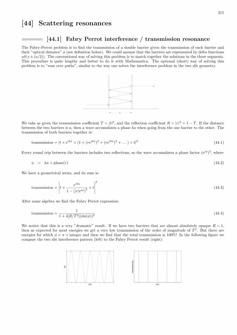
215

[44] Scattering resonances

====== [44.1] Fabry Perrot interference / transmission resonance

The Fabry-Perrot problem is to find the transmission of a double barrier given the transmission of each barrier andtheir ”optical distance” φ (see definition below). We could assume that the barriers are represented by delta functionsuδ(x± (a/2)). The conventional way of solving this problem is to match together the solutions in the three segments.This procedure is quite lengthy and better to do it with Mathematica. The optional (short) way of solving thisproblem is to ”sum over paths”, similar to the way one solves the interference problem in the two slit geometry.

L

We take as given the transmission coefficient T = |t|2, and the reflection coefficient R = |r|2 = 1− T . If the distancebetween the two barriers is a, then a wave accumulates a phase ka when going from the one barrier to the other. Thetransmission of both barriers together is:

transmission = |t× eika × (1 + (reika)2 + (reika)4 + . . . )× t|2 (44.1)

Every round trip between the barriers includes two reflections, so the wave accumulates a phase factor (eiφ)2, where

φ = ka+ phase(r) (44.2)

We have a geometrical series, and its sum is:

transmission =

∣∣∣∣∣t× eika

1− (|r|eiφ)2 × t

∣∣∣∣∣2

(44.3)

After some algebra we find the Fabry Perrot expression:

transmission =1

1 + 4[R/T 2](sin(φ))2(44.4)

We notice that this is a very ”dramatic” result. If we have two barriers that are almost absolutely opaque R ∼ 1,then as expected for most energies we get a very low transmission of the order of magnitude of T 2. But there areenergies for which φ = π × integer and then we find that the total transmission is 100%! In the following figure wecompare the two slit interference pattern (left) to the Fabry Perrot result (right):

−5 −4 −3 −2 −1 0 1 2 3 4 50

1

2

φ(π)

I(φ)

−2 −1 0 1 2

φ(π)

trans

miss

ion(

φ)

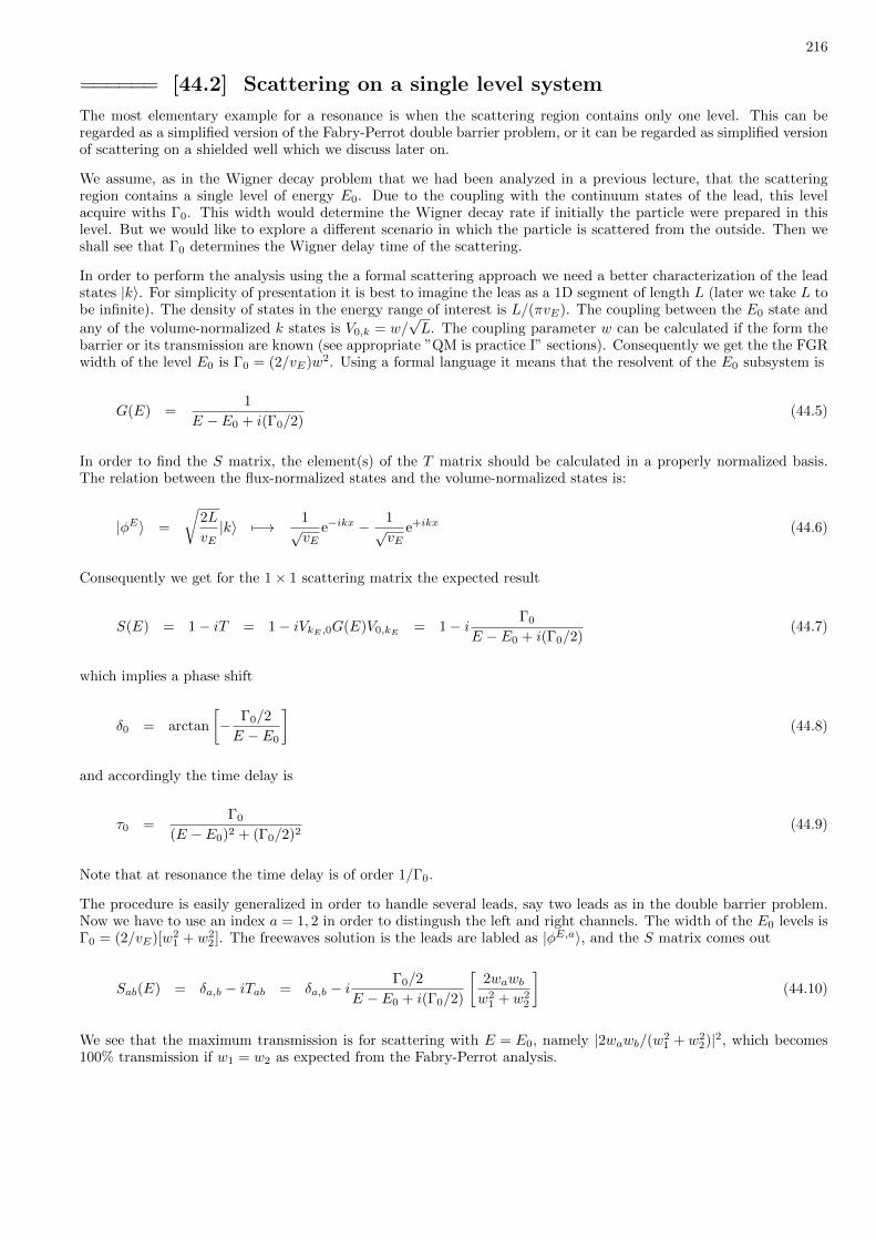
216

====== [44.2] Scattering on a single level system

The most elementary example for a resonance is when the scattering region contains only one level. This can beregarded as a simplified version of the Fabry-Perrot double barrier problem, or it can be regarded as simplified versionof scattering on a shielded well which we discuss later on.

We assume, as in the Wigner decay problem that we had been analyzed in a previous lecture, that the scatteringregion contains a single level of energy E0. Due to the coupling with the continuum states of the lead, this levelacquire withs Γ0. This width would determine the Wigner decay rate if initially the particle were prepared in thislevel. But we would like to explore a different scenario in which the particle is scattered from the outside. Then weshall see that Γ0 determines the Wigner delay time of the scattering.

In order to perform the analysis using the a formal scattering approach we need a better characterization of the leadstates |k〉. For simplicity of presentation it is best to imagine the leas as a 1D segment of length L (later we take L tobe infinite). The density of states in the energy range of interest is L/(πvE). The coupling between the E0 state and

any of the volume-normalized k states is V0,k = w/√L. The coupling parameter w can be calculated if the form the

barrier or its transmission are known (see appropriate ”QM is practice I” sections). Consequently we get the the FGRwidth of the level E0 is Γ0 = (2/vE)w2. Using a formal language it means that the resolvent of the E0 subsystem is

G(E) =1

E − E0 + i(Γ0/2)(44.5)

In order to find the S matrix, the element(s) of the T matrix should be calculated in a properly normalized basis.The relation between the flux-normalized states and the volume-normalized states is:

|φE〉 =

√2L

vE|k〉 7−→ 1

√vE

e−ikx − 1√vE

e+ikx (44.6)

Consequently we get for the 1× 1 scattering matrix the expected result

S(E) = 1− iT = 1− iVkE ,0G(E)V0,kE = 1− i Γ0

E − E0 + i(Γ0/2)(44.7)

which implies a phase shift

δ0 = arctan

[− Γ0/2

E − E0

](44.8)

and accordingly the time delay is

τ0 =Γ0

(E − E0)2 + (Γ0/2)2(44.9)

Note that at resonance the time delay is of order 1/Γ0.

The procedure is easily generalized in order to handle several leads, say two leads as in the double barrier problem.Now we have to use an index a = 1, 2 in order to distingush the left and right channels. The width of the E0 levels isΓ0 = (2/vE)[w2

1 + w22]. The freewaves solution is the leads are labled as |φE,a〉, and the S matrix comes out

Sab(E) = δa,b − iTab = δa,b − iΓ0/2

E − E0 + i(Γ0/2)

[2wawbw2

1 + w22

](44.10)

We see that the maximum transmission is for scattering with E = E0, namely |2wawb/(w21 + w2

2)|2, which becomes100% transmission if w1 = w2 as expected from the Fabry-Perrot analysis.

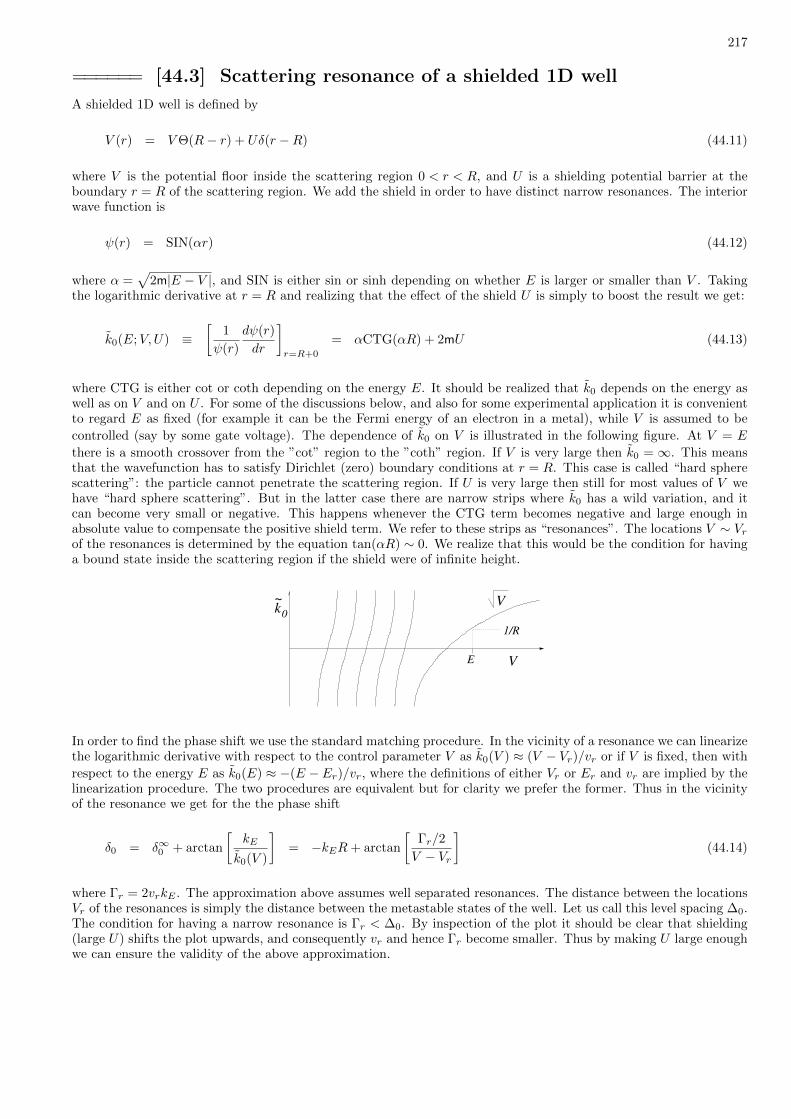
217

====== [44.3] Scattering resonance of a shielded 1D well

A shielded 1D well is defined by

V (r) = VΘ(R− r) + Uδ(r −R) (44.11)

where V is the potential floor inside the scattering region 0 < r < R, and U is a shielding potential barrier at theboundary r = R of the scattering region. We add the shield in order to have distinct narrow resonances. The interiorwave function is

ψ(r) = SIN(αr) (44.12)

where α =√

2m|E − V |, and SIN is either sin or sinh depending on whether E is larger or smaller than V . Takingthe logarithmic derivative at r = R and realizing that the effect of the shield U is simply to boost the result we get:

k0(E;V,U) ≡[

1

ψ(r)

dψ(r)

dr

]r=R+0

= αCTG(αR) + 2mU (44.13)

where CTG is either cot or coth depending on the energy E. It should be realized that k0 depends on the energy aswell as on V and on U . For some of the discussions below, and also for some experimental application it is convenientto regard E as fixed (for example it can be the Fermi energy of an electron in a metal), while V is assumed to be

controlled (say by some gate voltage). The dependence of k0 on V is illustrated in the following figure. At V = E

there is a smooth crossover from the ”cot” region to the ”coth” region. If V is very large then k0 = ∞. This meansthat the wavefunction has to satisfy Dirichlet (zero) boundary conditions at r = R. This case is called “hard spherescattering”: the particle cannot penetrate the scattering region. If U is very large then still for most values of V wehave “hard sphere scattering”. But in the latter case there are narrow strips where k0 has a wild variation, and itcan become very small or negative. This happens whenever the CTG term becomes negative and large enough inabsolute value to compensate the positive shield term. We refer to these strips as “resonances”. The locations V ∼ Vrof the resonances is determined by the equation tan(αR) ∼ 0. We realize that this would be the condition for havinga bound state inside the scattering region if the shield were of infinite height.

k

V

1/R

V0

E

~

In order to find the phase shift we use the standard matching procedure. In the vicinity of a resonance we can linearizethe logarithmic derivative with respect to the control parameter V as k0(V ) ≈ (V − Vr)/vr or if V is fixed, then with

respect to the energy E as k0(E) ≈ −(E − Er)/vr, where the definitions of either Vr or Er and vr are implied by thelinearization procedure. The two procedures are equivalent but for clarity we prefer the former. Thus in the vicinityof the resonance we get for the the phase shift

δ0 = δ∞0 + arctan

[kE

k0(V )

]= −kER+ arctan

[Γr/2

V − Vr

](44.14)

where Γr = 2vrkE . The approximation above assumes well separated resonances. The distance between the locationsVr of the resonances is simply the distance between the metastable states of the well. Let us call this level spacing ∆0.The condition for having a narrow resonance is Γr < ∆0. By inspection of the plot it should be clear that shielding(large U) shifts the plot upwards, and consequently vr and hence Γr become smaller. Thus by making U large enoughwe can ensure the validity of the above approximation.

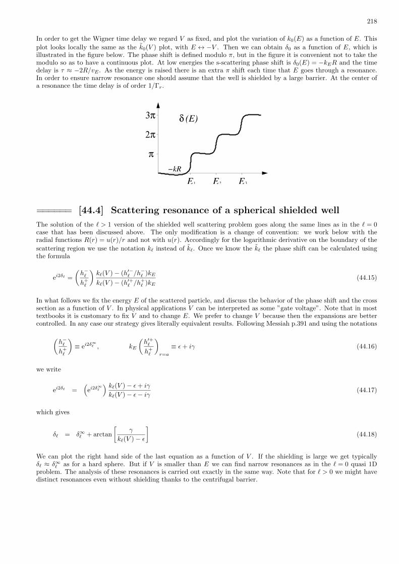
218

In order to get the Wigner time delay we regard V as fixed, and plot the variation of k0(E) as a function of E. This

plot looks locally the same as the k0(V ) plot, with E ↔ −V . Then we can obtain δ0 as a function of E, which isillustrated in the figure below. The phase shift is defined modulo π, but in the figure it is convenient not to take themodulo so as to have a continuous plot. At low energies the s-scattering phase shift is δ0(E) = −kER and the timedelay is τ ≈ −2R/vE . As the energy is raised there is an extra π shift each time that E goes through a resonance.In order to ensure narrow resonance one should assume that the well is shielded by a large barrier. At the center ofa resonance the time delay is of order 1/Γr.

3π

2π

π

δ (E)

−kR1E 3E2E

====== [44.4] Scattering resonance of a spherical shielded well

The solution of the ` > 1 version of the shielded well scattering problem goes along the same lines as in the ` = 0case that has been discussed above. The only modification is a change of convention: we work below with theradial functions R(r) = u(r)/r and not with u(r). Accordingly for the logarithmic derivative on the boundary of the

scattering region we use the notation k` instead of k`. Once we know the k` the phase shift can be calculated usingthe formula

ei2δ` =

(h−`h+`

)k`(V )− (h′−` /h

−` )kE

k`(V )− (h′+` /h+` )kE

(44.15)

In what follows we fix the energy E of the scattered particle, and discuss the behavior of the phase shift and the crosssection as a function of V . In physical applications V can be interpreted as some ”gate voltage”. Note that in mosttextbooks it is customary to fix V and to change E. We prefer to change V because then the expansions are bettercontrolled. In any case our strategy gives literally equivalent results. Following Messiah p.391 and using the notations

(h−`h+`

)≡ ei2δ

∞` , kE

(h′+`h+`

)r=a

≡ ε+ iγ (44.16)

we write

ei2δ` =(

ei2δ∞`

) k`(V )− ε+ iγ

k`(V )− ε− iγ(44.17)

which gives

δ` = δ∞` + arctan

[γ

k`(V )− ε

](44.18)

We can plot the right hand side of the last equation as a function of V . If the shielding is large we get typicallyδ` ≈ δ∞` as for a hard sphere. But if V is smaller than E we can find narrow resonances as in the ` = 0 quasi 1Dproblem. The analysis of these resonances is carried out exactly in the same way. Note that for ` > 0 we might havedistinct resonances even without shielding thanks to the centrifugal barrier.

219

QM in Practice (part III)

[45] The Aharonov-Bohm effect

====== [45.1] The Aharonov-Bohm geometry

In the quantum theory it is natural to describe the electromagnetic field using the potentials V,A and regard E ,Bas associated observables. Below we discuss the case in which E = B = 0 in the region where the particle is moving.According to the classical theory one expects that the motion of the particle would not be affected by the field, sincethe Lorentz force is zero. However, we shall see that according to the quantum theory the particle is affected due tothe non-zero circulation of A. This is a topological effect that we are going to clarify. Specifically we consider ringthat is penetrated by a magnetic flux Φ through its center. This is the so-called Aharonov-Bohm geometry. To havea flux through the ring means that:

∮~A · d~l =

xB · d~s = Φ (45.1)

The simplest gauge choice for the vector potential is

A =Φ

L[tangential] (45.2)

where L is the length of the ring. Below we treat the ring as a 1D segment 0 < x < L with periodic boundaryconditions. The Hamiltonian is

H =1

2m

(p− eΦ

cL

)2

(45.3)

The eigenstates of H are the momentum states |kn〉 where:

kn =2π

Ln, n = 0,±1,±2, ... (45.4)

The eigenvalues are (written with ~ for historical reasons):

En =1

2m

(2π~Ln− eΦ

cL

)2

=1

2m

(2π~L

)2(n− eΦ

2π~c

)2

(45.5)

The unit 2π~c/e is called ”fluxon”. It is the basic unit of flux in nature. We see that the energy spectrum is influencedby the presence of the magnetic flux. On the other hand, if we draw a plot of the energies as a function of the flux wesee that the energy spectrum repeats itself every time the change in the flux is an integer multiple of a fluxon. (Toguide the eye we draw the ground state energy with thick line).

The fact that the electron is located in an area where there is no Lorentz force E = B = 0, but is still influenced bythe vector potential is called the Aharonov-Bohm Effect. This is an example of a topological effect.

220

Φ

−3 −2 −1 0 1 2 3

Φ [fluxons]

E n(Φ)

====== [45.2] The energy levels of a ring with a scatterer

Consider an Aharonov-Bohm ring with (say) a delta scatterer:

H =1

2m

(p− eΦ

L

)2

+ uδ(x) (45.6)

We would like to find the eigenenergies of the ring. The standard approach is to write the general solution in theempty segment, and then to impose the matching condition over the delta scatterer. An elegant procedure for solutionis based on the scattering formalism. In order to characterize the scattering within the system, the ring is cut atsome arbitrary point and the S matrix of the open segment is specified. It is more convenient to use the row-swappedmatrix, such that the transmission amplitudes are along the diagonal:

S = eiγ( √

geiφ −i√

1− ge−iα

−i√

1− geiα√ge−iφ

)(45.7)

where the transmission is

g(E) =

[1 +

(u

vE

)2]−1

, vE = velocity at energy E (45.8)

We include “legs” to the delta scatterer, hence the total transmission phase is

γ(E) = kEL− arctan

(u

vE

)(45.9)

More precisely, with added flux the transmission phases are γ ± φ where φ = eΦ/~. The reflection phases areγ − (π/2)± α, where α = 0 if we cut the ring symmetrically, such that the two legs have the same length.

The periodic boundary conditions imply the ”matching condition”

(AB

)= S

(AB

)(45.10)

221

This equation has a non-trivial solution if and only if

det(S(E)− 1) = 0 (45.11)

For the calculation is is useful to note that

det(S− 1) = det(S)− trace(S) + 1 (45.12)

det(S) = (eiγ)2 (45.13)

trace(S) = 2√geiγ cosφ (45.14)

Hence we get an equation for the eigen-energies:

cos(γ(E)) =√g(E) cos(φ) (45.15)

In order to find the eigen-energies we plot both sides as a function of E. The left hand side oscillates between −1and +1, while the right hand side is slowly varying monotonically. It is easily verified that the expected results areobtained for clean ring (g = 1) and for infinite well (g = 0).

====== [45.3] Perturbation theory for a ring + scatterer

Let us consider a particle with mass m on a 1D ring. A flux Φ goes through the ring. In addition, there is a scattererthat is described by a delta function. The Hamiltonian that describes the system is:

H =1

2m

(p− Φ

L

)2

+ uδ(x) (45.16)

For Φ = u = 0 the symmetry group of this Hamiltonian is O(2). This means symmetry with respect to rotations andreflections. Note that in one-dimension ring = circle = torus, hence rotations and displacements are the same. Onlyin higher dimensions they are different (torus 6= sphere).

Degeneracies are an indication for symmetries of the Hamiltonian. If the eigenstate has a lower symmetry than theHamiltonian, a degeneracy appears. Rotations and reflections do not commute, that is why we have degeneracies.When we add flux or a scatterer, the degeneracies open up. Adding flux breaks the reflection symmetry, and addinga scatterer breaks the rotation symmetry. Accordingly, depending on the perturbation, it would be wise to use oneof the following two bases:

The first basis: The first basis complies with the rotation (=translations) symmetry:

|n = 0〉 =1√L

(45.17)

|n, anticlockwise〉 =1√L

e+iknx, n = 1, 2, ...

|n, clockwise〉 =1√L

e−iknx, n = 1, 2, ...

The degenerate states are different under reflection. Only the ground state |n = 0〉 is symmetric under both reflectionsand rotations, and therefore it does not have to be degenerate. It is very easy to calculate the perturbation matrixelements in this basis:

〈n|δ(x)|m〉 =

∫Ψn(x)δ(x)Ψm(x)dx = Ψn(0)Ψm(0) =

1

L(45.18)

222

so we get:

Vnm =u

L

1 1 1 1 . . .1 1 1 1 . . .1 1 1 1 . . .1 1 1 1 . . .. . . . . . . . . . . . . . .

(45.19)

The second basis: The second basis complies with the reflection symmetry:

|n = 0〉 =1√L

(45.20)

|n,+〉 =

√2

Lcos(knx), n = 1, 2, ...

|n,−〉 =

√2

Lsin(knx), n = 1, 2, ...

The degeneracy is between the even states and the odd states that are displaced by half a wavelength with respectto each other. If the perturbation is not the flux but rather the scatterer, then it is better to work with the secondbasis, which complies with the potential’s symmetry. The odd states are not influenced by the delta function, andthey are also not ”coupled” to the even states. The reason is that:

〈m|δ(x)|n〉 =

∫Ψm(x)δ(x)Ψn(x)dx = 0, if n or m are ”sin” (45.21)

Consequently the subspace of odd states is not influenced by the perturbation, i.e. V(−)nm = 0, and we only need to

diagonalize the block that belongs to the even states. It is very easy to write the perturbation matrix for this block:

V (+)nm =

u

L

1√

2√

2√

2 . . .√2 2 2 2 . . .√2 2 2 2 . . .√2 2 2 2 . . .

. . . . . . . . . . . . . . .

(45.22)

Energy levels: Without a scatterer the eigenenergies are:

En(Φ, u=0) =1

2m

(2π

L× integer− Φ

L

)2

, integer = 0,±1,±2, ... (45.23)

On the other hand, in the limit u→∞ the system does not ”feel” the flux, and the ring becomes a one-dimensionalbox. The eigenenergies in this limit are:

En(Φ, u=∞) =1

2m

(πL× integer

)2

, integer = 1, 2, ... (45.24)

As one increases u the number of the energy levels does not change, they just move. See figure below. We would liketo use perturbation theory in order to find corrections to the above expressions. We consider how we do perturbationtheory with respect to the u=0 Hamiltonian. It is also possible to carry out perturbation theory with respect to theu=∞ Hamiltonian (for that one should use the formula for the interaction at a junction).

223

9

4

10

16

En

u=− u=0 u=+

8 8

The corrections to the energy: Let us evaluate the first-order correction to the energy of the eigenstates in theabsence of an external flux.

En=0 = E[0]n=0 +

u

L(45.25)

En=2,4,... = E[0]n +

2u

L

The correction to the ground state energy, up to the second order is:

En=0 = 0 +u

L+( uL

)2 ∞∑k=1

(√

2)2

0− 12m

(2πL k)2 =

u

L

(1− 1

6umL

)(45.26)

where we have used the identity:

∞∑k=1

1

k2=

π2

6(45.27)

Optional calculation: We will now assume that we did not notice the symmetry of the problem, and we chose towork with the first basis. Using perturbation theory on the ground state energy is simple in this basis:

En=0 = 0 +u

L+( uL

)2

2

∞∑k=1

(1)2

0− 12m

(2πL k)2 =

u

L

(1− 1

6umL

)(45.28)

But using perturbation theory on the rest of the states is difficult because there are degeneracies. The first thing wemust do is ”degenerate perturbation theory”. The diagonalization of each degenerate energy level is:

(1 11 1

)→

(2 00 0

)(45.29)

Now we should transform to a new basis, where the degeneracy is removed. This is exactly the basis that we choseto work with due to symmetry considerations. The moral lesson is: understanding the symmetries in the system cansave us work in the calculations of perturbation theory.

224

====== [45.4] The AB effect in a closed geometry

The eigen-energies of a particle in a closed ring are periodic functions of the flux. In particular in the absence ofscattering

En =1

2m

(2π~L

)2(n− eΦ

2π~c

)2

=1

2mv2

n (45.30)

That is in contrast with classical mechanics, where the energy can have any positive value:

Eclassical =1

2mv2 (45.31)

According to classical mechanics the lowest energy of a particle in a magnetic field is zero, with velocity zero. Thisis not true in the quantum case. It follows that an added magnetic flux has an detectable effect on the system. Theeffect can be described in one of the following ways:

• The spectrum of the system changes (it can be measured using spectroscopy)• For flux that is not an integer or half integer number there are persistent currents in the system.• The system has either a diamagnetic or a paramagnetic response (according to the occupancy).

We already have discussed the spectrum of the system. So the next thing is to derive an expression for the current inthe ring. The current operator is

I ≡ −∂H∂Φ

=e

L

[1

m

(p− eΦ

L

)]=

e

Lv (45.32)

It follows that the current which is created by an electron that occupies the nth level is:

In =

⟨n

∣∣∣∣(−∂H∂Φ

)∣∣∣∣n⟩ = −dEndΦ

(45.33)

The proof of the second equality is one line of algebra. If follows that by looking at the plot of the energies En(Φ)as a function of the flux, one can determine (according to the slope) what is the current that flows in each occupiedenergy level. If the flux is neither integer nor half integer, all the states ”carry current” so that in equilibrium the netcurrent is not zero. This phenomenon is called ”persistent currents”. The equilibrium current in such case cannotrelax to zero, even if the temperature of the system is zero.

There is a statement in classical statistical mechanics that the equilibrium state of a system is not affected by magneticfields. The magnetic response of any system is a quantum mechanical effect that has to do with the quantization ofthe energy levels (Landau magnetism) or with the spins (Pauly magnetism). Definitions:

• Diamagnetic System - in a magnetic field, the system energy increases.• Paramagnetic System - in a magnetic field, the system energy decreases.

The Aharonov Bohm geometry provides the simplest example for magnetic response. If we place one electron in a ring,and add a weak magnetic flux, the system energy increases. Accordingly we say that the response is ”diamagnetic”.The electron cannot ”get rid” of its kinetic energy, because of the quantization of the momentum.

225

====== [45.5] Dirac Monopoles

Yet another consequence of the ”Aharonov Bohm” effect is the quantization of the magnetic charge. Dirac has claimedthat if magnetic monopoles exist, then there must be an elementary magnetic charge. The formal argument can bephrased as follows: If a magnetic monopole exists, it creates a vector potential field in space (A(x)). The effect of the

field of the monopole on an electron close by is given by the line integral∮~A · d~r. We can evaluate the integral by

calculating the magnetic flux Φ through a Stokes surface. The result should not depend on the choice of the surface,otherwise the phase is not be well defined. In particular we can choose Stokes surfaces that pass above and below themonopole, and deduce that the phase difference φ = eΦ/~c should be zero modulo 2π. Hence the flux Φ should be aninteger multiple of 2π~c/e. Using ”Gauss law” we conclude that the monopole must have a magnetic charge that isquantized in units of ~c/2e.

Dirac’s original reasoning was somewhat more constructive. Let us assume that a magnetic monopole exist. Themagnetic field that would be created by this monopole would be like that of a tip of a solenoid. But we have toexclude the region in space where we have the magnetic flux that goes through the solenoid. If we want this ”fluxline” to be unobservable then it should be quantized in units of 2π~c/e. This shows that Dirac ”heard” about theAharonov Bohm effect, but more importantly this implies that the ”tip” would have a charge which equals an integermultiple of ~c/2e.

====== [45.6] The AB effect: path integral formulation

We can optionally illustrate the Aharonov-Bohm Effect by considering an open geometry. In an open geometry theenergy is not quantized: it is determined by scattering arrangement. If the energy potential floor is taken as a reference- the energy E can be any positive value. We are looking for stationary states that solve the Schrodinger equationfor a given energy. These states are called ”scattering states”. Below we discuss the Aharonov-Bohm effect in a ”twoslit” geometry, and later refer to a ”ring” geometry (with leads).

First we notice the following rule: if we have a planar wave ψ(x) ∝ eikx, and if the amplitude at the point x = x1 isψ(x1) = C, then at another point x = x2 the amplitude is ψ(x2) = Ceik(x2−x1).

Now we generalize this rule for the case in which there is a vector potential A. For simplicity, we assume that themotion is in one-dimension. The eigenstates of the Hamiltonian are the momentum states. If the energy of the particleis E then the wavefunctions that solve the Schrodinger’s equation are ψ(x) ∝ eik±x, where

k± = ±√

2mE +A ≡ ±kE +A (45.34)

Below we refer to the advancing wave: if at point x = x1 the amplitude is ψ(x1) = C, then at another point x = x2

the amplitude is ψ(x2) = CeikE(x2−x1)+A·(x2−x1). It is possible to generalize the idea to three dimensions: if a waveadvances along a certain path from point x1 to point x2, then the accumulated phase is:

φ = kEL+

∫ x2

x1

A · dx, L = length of the path (45.35)

If there are two different paths that connect the points x1 and x2, then the phase difference is:

∆φ = kE∆L+

∫L2

A · dx−∫L1

A · dx = kE∆L+

∮A · dx = kE∆L+

e

~cΦ (45.36)

where in the last term we ”bring back” the standard physical units. The approach which was presented above forcalculating the probability of the particle to go from one point to another is called ”path integrals”. This approachwas developed by Feynman, and it leads to what is called ”path integral formalism” - an optional approach todo calculations in quantum mechanics. The conventional method is to solve the Schrodinger’s equation with theappropriate boundary conditions.

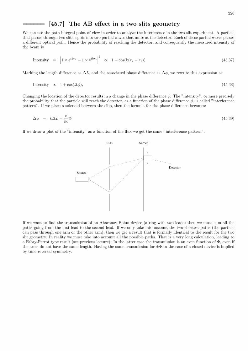
226

====== [45.7] The AB effect in a two slits geometry

We can use the path integral point of view in order to analyze the interference in the two slit experiment. A particlethat passes through two slits, splits into two partial waves that unite at the detector. Each of these partial waves passesa different optical path. Hence the probability of reaching the detector, and consequently the measured intensity ofthe beam is

Intensity =∣∣∣1× eikr1 + 1× eikr2

∣∣∣2 ∝ 1 + cos(k(r2 − r1)) (45.37)

Marking the length difference as ∆L, and the associated phase difference as ∆φ, we rewrite this expression as:

Intensity ∝ 1 + cos(∆φ), (45.38)

Changing the location of the detector results in a change in the phase difference φ. The ”intensity”, or more preciselythe probability that the particle will reach the detector, as a function of the phase difference φ, is called ”interferencepattern”. If we place a solenoid between the slits, then the formula for the phase difference becomes:

∆φ = k∆L+e

~cΦ (45.39)

If we draw a plot of the ”intensity” as a function of the flux we get the same ”interference pattern”.

Detector

Slits Screen

Source

If we want to find the transmission of an Aharonov-Bohm device (a ring with two leads) then we must sum all thepaths going from the first lead to the second lead. If we only take into account the two shortest paths (the particlecan pass through one arm or the other arm), then we get a result that is formally identical to the result for the twoslit geometry. In reality we must take into account all the possible paths. That is a very long calculation, leading toa Fabry-Perrot type result (see previous lecture). In the latter case the transmission is an even function of Φ, even ifthe arms do not have the same length. Having the same transmission for ±Φ in the case of a closed device is impliedby time reversal symmetry.

227

[46] Motion in uniform magnetic field (Landau, Hall)

====== [46.1] The two-dimensional ring geometry

Let us consider a three-dimensional box with periodic boundary conditions in the x direction, and zero boundaryconditions on the other sides. In the absence of magnetic field we assume that the Hamiltonian is:

H =1

2mp2x +

[1

2mp2y + V (y)

]+

[1

2mp2z + Vbox(z)

](46.1)

The eigenstates of a particle in such box are labeled as

|kx, ny, nz〉 (46.2)

kx =2π

L× integer

ny, nz = 1, 2, 3 . . .

The eigenenergies are:

Ekx,ny,nz =k2x

2m+ εny +

1

2m

(π

Lznz

)2

(46.3)

We assume Lz to be very small compared to the other dimensions. We shall discuss what happens when the systemis prepared in low energies such that only nz = 1 states are relevant. So we can ignore the z axis.

====== [46.2] Classical Motion in a uniform magnetic field

Consider the motion of an electron in a two-dimensional ring. We assume that the vertical dimension is ”narrow”, sothat we can safely ignore it, as was explained in the previous section. For convenience we ”spread out” the ring suschthat it forms a rectangle with periodic boundary conditions over 0 < x < Lx, and an arbitrary confining potentialV (y) in the perpendicular direction. Additionally we assume that there is a uniform magnetic field B along the z axis.Therefore the electron is affected by a Lorentz force F = −(e/c)B × v. If there is no electrical potential, the electronperforms a circular motion with the cyclotron frequency:

ωB =eBmc

(46.4)

If the electron has a kinetic energy E, its velocity is:

vE =

√2E

m(46.5)

Consequently it moves along a circle of radius

rE =vEωB

=mc

eBvE (46.6)

If we take into account a non-zero electric field

Ey = −dVdy

(46.7)

228

we get a motion along a cycloid with the drift velocity (see derivation below):

vdrift = cEyB

(46.8)

Let us remind ourselves why the motion is along a cycloid. The Lorentz force in the laboratory reference frame is(from now on we absorb the (e/c) of the electron into the definition of the field):

F = E − B × v (46.9)

If we transform to a reference frame that is moving at a velocity v0 we get:

F = E − B × (v′ + v0) = (E + v0 × B)− B × v′ (46.10)

Therefore, the non-relativistic transformation of the electromagnetic field is:

E ′ = E + v0 × B (46.11)

B′ = B

If there is a field in the y direction in the laboratory reference frame, we can transform to a new reference frame wherethe field is zero. From the transformation above we conclude that in order to have a zero electrical field, the velocityof the ”new” frame of reference should be:

v0 =EBc [restoring CGS units for clarity] (46.12)

In the new reference frame the particle moves along a circle. Therefore, in the laboratory reference frame it movesalong a cycloid.

x

y

(x,y) (v ,v )x y

(X,Y)

Conventionally the classical state of the particle is described by the coordinates r = (x, y) and v = (vx, vy). But fromthe above discussion it follows that a simpler description of the trajectory is obtained if we follow the motion of themoving circle. The center of the circle R = (X,Y ) is moving along a straight line, and its velocity is vdrift. Thetransformation that relates R to r and v is

~R = ~r − ~ez ×1

ωB~v (46.13)

where ~ez is a unit vector in the z direction. The second term in the right hand side is a vector of length rE in theradial direction (perpendicular to the velocity). Thus instead of describing the motion with the canonical coordinates(x, y, vx, vy), we can use the new coordinated (X,Y, vx, vy).

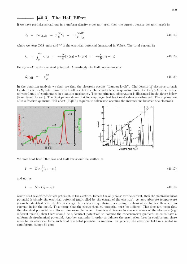
229

====== [46.3] The Hall Effect

If we have particles spread out in a uniform density ρ per unit area, then the current density per unit length is:

Jx = eρvdrift = ρec

BEy = −ρec

BdV

dy(46.14)

where we keep CGS units and V is the electrical potential (measured in Volts). The total current is:

Ix =

∫ y2

y1

Jxdy = −ρecB

(V (y2)− V (y1)) = −ρ cB

(µ2 − µ1) (46.15)

Here µ = eV is the chemical potential. Accordingly the Hall conductance is:

GHall = −ρecB

(46.16)

In the quantum analysis we shall see that the electrons occupy ”Landau levels”. The density of electrons in eachLandau Level is eB/2π~c. From this it follows that the Hall conductance is quantized in units of e2/2π~, which is theuniversal unit of conductance in quantum mechanics. The experimental observation is illustrated in the figure below[taken from the web]. The right panels shows that for very large field fractional values are observed. The explanationof this fraction quantum Hall effect (FQHE) requires to taken into account the interactions between the electrons.

We note that both Ohm law and Hall law should be written as:

I = G× 1

e(µ2 − µ1) (46.17)

and not as:

I = G× (V2 − V1) (46.18)

where µ is the electrochemical potential. If the electrical force is the only cause for the current, then the electrochemicalpotential is simply the electrical potential (multiplied by the charge of the electron). At zero absolute temperatureµ can be identified with the Fermi energy. In metals in equilibrium, according to classical mechanics, there are nocurrents inside the metal. This means that the electrochemical potential must be uniform. This does not mean thatthe electrical potential is uniform! For example: when there is a difference in concentrations of the electrons (e.g.different metals) then there should be a ”contact potential” to balance the concentration gradient, so as to have auniform electrochemical potential. Another example: in order to balance the gravitation force in equilibrium, theremust be an electrical force such that the total potential is uniform. In general, the electrical field in a metal inequilibrium cannot be zero.

230

====== [46.4] Electron in Hall geometry: Landau levels

In this section we show that there is an elegant formal way of treating the problem of an electron in Hall geometry usinga canonical transformation. This method of solution is valid both in classical mechanics and in quantum mechanics(all one has to do is to replace the Poisson brackets with commutators). In the next lecture we solve the quantumproblem again, using the conventional method of ”separation of variables”. Here and later we use the Landau gauge:

~A = (−By, 0, 0) (46.19)

B = ∇× ~A = (0, 0,B)

Recall that we absorb the charge of the electron in the definition of the fields. Consequently the Hamiltonian is

H =1

2m(px + By)2 +

1

2m(py)2 + V (y) (46.20)

We define a new set of operators:

vx =1

m(px + By) (46.21)

vy =1

mpy

X = x+1

ωBvy = x+

1

Bpy

Y = y − 1

ωBvx = − 1

Bpx

Recall that from a geometrical perspective, (X,Y ) represent the center of the circle along which the particle is moving.Note also that the operators X,Y commute with vx, vy. On the other hand:

[X,Y ] = −iB−1 (46.22)

[vx, vy] = i1

m2B

Consequently we can define a new set of canonical coordinates:

Q1 =m

Bvx, P1 = mvy, Q2 = Y, P2 = BX (46.23)

The Hamiltonian takes the form

H(Q1, P1, Q2, P2) =1

2mP 2

1 +1

2mω2

BQ21 + V (Q1 +Q2) (46.24)

We see, as expected, that Q2 = Y is a constant of motion. Let us further assume that the potential V (y) is zerowithin a large box of area LxLy. Then also P2 ∝ X is a constant of motion. The coordinates (X,Y ) are conjugatewith ~B = B−1 and therefore we deduce that there are gLandau states that have the same energy, where

gLandau =LxLy2π~B

=LxLy

2πB (46.25)

Later we shall explain that it leads to the e2/(2π~) quantization of the Hall conductance. Beside the (X,Y ) degreeof freedom we have of course the kinetic (vx, vy) degree of freedom. Form the transformed Hamiltonian in the newcoordinates we clearly see that the kinetic energy is quantized in units of ωB . Therefore, it is natural to label the

231

eigenstates as |`, ν〉, where: ν = 0, 1, 2, 3 . . ., is the kinetic energy index, and ` labels the possible values of the constantof motion Y .

====== [46.5] Electron in Hall geometry: The Landau states

We go back to the Hamiltonian that describes the motion of a particle in the Hall bar geometry (see beginningof previous section). Recall that we have periodic boundary conditions in the x axis, and an arbitrary confiningpotential V (y) in the y direction. We would like to find the eigenstates and the eigenvalues of the Hamiltonian. Thekey observation is that in the Landau gauge the momentum operator px is a constant of motion. It is more physicalto re-phrase this statement in a gauge independent way. Namely, the constant of motion is in fact

Y = y − 1

ωBvx = − 1

Bpx (46.26)

which represents the y location of the classical cycloid. In fact the eigenstates that we are going to find are thequantum mechanical analogue of the classical cycloids. The eigenvalues of px are 2π/Lx × integer. Equivalently, we

may write that the eigenvalues of Y are:

Y` =2π

BLx`, [` = integer] (46.27)

That means that the y distance between the eigenstates is quantized. According to the ”separation of variablestheorem” the Hamiltonian matrix is a block diagonal matrix in the basis in which the Y matrix is diagonal. It isnatural to choose the basis |`, y〉 which is determined by the operators px, y.

〈`, y|H|`′, y′〉 = δ`,`′ H`yy′ (46.28)

It is convenient to write the Hamiltonian of the block ` in abstract notation (without indexes):

H` =1

2mp2y +B2

2m(y − Y`)2 + V (y) (46.29)

Or, in another notation:

H` =1

2mp2y + V`(y) (46.30)

where the effective potential is:

V`(y) = V (y) +1

2mω2B(y − Y`)2 (46.31)

For a given `, we find the eigenvalues |`, ν〉 of the one-dimensional Hamiltonian H`. The running index ν = 0, 1, 2, 3, . . .indicates the quantized values of the kinetic energy.

For a constant electric field we notice that this is the Schrodinger equation of a displaced harmonic oscillator. Moregenerally, the harmonic approximation for the effective potential is valid if the potential V (y) is wide compared tothe quadratic potential which is contributed by the magnetic field. In other words, we assume that the magnetic fieldis strong. We write the wave functions as:

|`, ν〉 → 1√Lx

e−i(BY`)x ϕ(ν)(y − Y`) (46.32)

We notice that BY` are the eigenvalues of the momentum operator. If there is no electrical field then the harmonicapproximation is exact, and then ϕ(ν) are the eigenfunctions of a harmonic oscillator. In the general case, we must

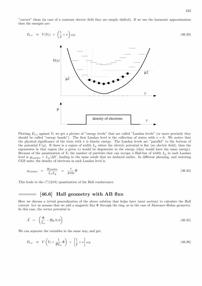
232

”correct” them (in case of a constant electric field they are simply shifted). If we use the harmonic approximationthen the energies are:

E`,ν ≈ V (Y`) +

(1

2+ ν

)ωB (46.33)

y

V(y)

µ1

µ2

y

ρ

density of electrons

Plotting E`,ν against Y` we get a picture of ”energy levels” that are called ”Landau levels” (or more precisely theyshould be called ”energy bands”). The first Landau level is the collection of states with ν = 0. We notice thatthe physical significance of the term with ν is kinetic energy. The Landau levels are ”parallel” to the bottom ofthe potential V (y). If there is a region of width Ly where the electric potential is flat (no electric field), then theeigenstates in that region (for a given ν) would be degenerate in the energy (they would have the same energy).Because of the quantization of Y` the number of particles that can occupy a Hall-bar of width Ly in each Landaulevel is gLandau = Ly/∆Y , leading to the same result that we deduced earlier. In different phrasing, and restoringCGS units, the density of electrons in each Landau level is

ρLandau =gLandau

LxLy=

e

2π~cB (46.34)

This leads to the e2/(2π~) quantization of the Hall conductance.

====== [46.6] Hall geometry with AB flux

Here we discuss a trivial generalization of the above solution that helps later (next section) to calculate the Hallcurrent. Let us assume that we add a magnetic flux Φ through the ring, as in the case of Aharonov-Bohm geometry.In this case, the vector potential is:

~A =

(Φ

Lx− By, 0, 0

)(46.35)

We can separate the variables in the same way, and get:

E`,ν ≈ V

(Y` +

1

BLxΦ

)+

[1

2+ ν

]ωB (46.36)

233

====== [46.7] The Quantum Hall current

We would like to calculate the current for an electron that occupies a Landau state |`, ν〉:

Jx(x, y) =1

2(vxδ(x− x)δ(y − y) + h.c.) (46.37)

Jx(y) =1

Lx

∫Jx(x, y)dx =

1

Lxvxδ(y − y)

Ix = −∂H∂Φ

=1

Lxvx =

∫Jx(y)dy

Recall that vx = (B/m)(y − Y ), and that the Landau states are eigenstates of Y . Therefore, the current density ofan occupied state is given by:

Jν`x (y) = 〈`ν|Jx(y)|`ν〉 =BLxm

⟨(y − Y ) δ(y − y)

⟩=

BmLx

(y − Y`) |ϕν(y − Y`)|2 (46.38)

If we are in the region (Y` < y) we observe current that flows to the right (in the direction of the positive x axis), andthe opposite if we are on the other side. This is consistent with the classical picture of a particle moving clockwise ina circle. If there is no electric field, the wave function is symmetric around Y`, so we get zero net current. If thereis a non-zero electric field, it shifts the wave function and then we get a net current that is not zero. The current isgiven by:

I`νx =

∫J`νx (y)dy = −∂E`ν

∂Φ= − 1

BLxdV (y)

dy

∣∣∣∣y=Y`

(46.39)

For a Fermi occupation of the Landau level we get:

Ix =∑`

I`νx =

∫ y2

y1

dy

2π/(BLx)

(− 1

BLxdV (y)

dy

)(46.40)

= − 1

2π(V (y2)− V (y1)) = − e

2π~(µ2 − µ1)

In the last equation we have restored the standard physical units. We see that if there is a chemical potential differencewe get a current Ix. Writing µ = eV , the Hall coefficient is e2/(2π~) times the number of full Landau levels.

====== [46.8] Hall effect and adiabtic transport

The calculation of the Hall conductance is possibly the simplest non-trivial example for adiabatic non-dissipativeresponse. The standard geometry is the 2D ”hall bar” of dimension Lx × Ly. We have considered what happensif the electrons are confined in the transverse direction by a potential V (y). Adopting the Landauer approach it isassumed that the edges are connected to leads that maintain a chemical potential difference. Consequently there is anet current in the x direction. From the ”Landau level” picture it is clear that the Hall conductance Gxy is quantizedin units e2/(2π~). The problem with this approach is that the more complicated case of disordered V (x, y) is difficultfor handling. We therefore turn to a formal linear response approach [see section 22]. From now on we use units suchthat e = ~ = 1.

We still consider a Hall bar Lx × Ly, but now we impose periodic boundary condition such that ψ(Lx, y) = eiφxψ(0, y)and ψ(x, Ly) = eiφyψ(x, 0). Accordingly the Hamiltonian depends on the parameters (φx, φy,ΦB), where ΦB is theuniform magnetic flux through the Hall bar in the z direction. The currents Ix = (e/Lx)vx and Iy = (e/Ly)vyare conjugate to φx and φy. We consider the linear response relation Iy = −Gyxφx. This relation can be written asdQy = −Gyxdφx. The Hall conductance quantization means that a 2π variation of φx leads to one particle transportedin the y direction. The physical picture is very clear in the standard V (y) geometry: the net effect is to displace allthe filled Landau level ”one step” in the y direction.

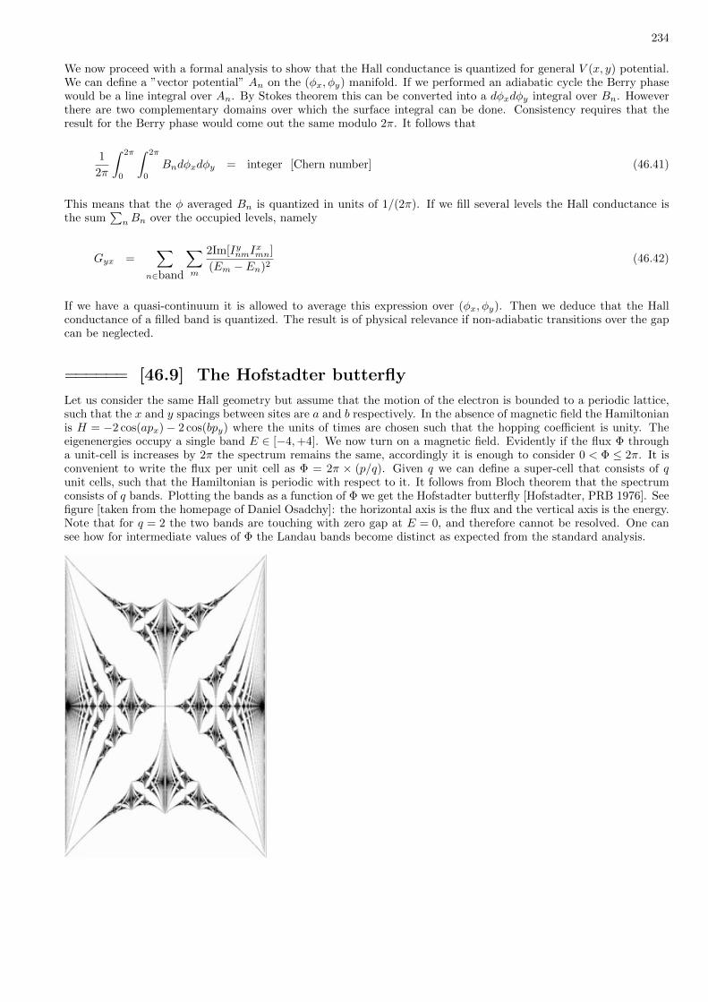
234

We now proceed with a formal analysis to show that the Hall conductance is quantized for general V (x, y) potential.We can define a ”vector potential” An on the (φx, φy) manifold. If we performed an adiabatic cycle the Berry phasewould be a line integral over An. By Stokes theorem this can be converted into a dφxdφy integral over Bn. Howeverthere are two complementary domains over which the surface integral can be done. Consistency requires that theresult for the Berry phase would come out the same modulo 2π. It follows that

1

2π

∫ 2π

0

∫ 2π

0

Bndφxdφy = integer [Chern number] (46.41)

This means that the φ averaged Bn is quantized in units of 1/(2π). If we fill several levels the Hall conductance isthe sum

∑nBn over the occupied levels, namely

Gyx =∑

n∈band

∑m

2Im[IynmIxmn]

(Em − En)2(46.42)

If we have a quasi-continuum it is allowed to average this expression over (φx, φy). Then we deduce that the Hallconductance of a filled band is quantized. The result is of physical relevance if non-adiabatic transitions over the gapcan be neglected.

====== [46.9] The Hofstadter butterfly

Let us consider the same Hall geometry but assume that the motion of the electron is bounded to a periodic lattice,such that the x and y spacings between sites are a and b respectively. In the absence of magnetic field the Hamiltonianis H = −2 cos(apx)− 2 cos(bpy) where the units of times are chosen such that the hopping coefficient is unity. Theeigenenergies occupy a single band E ∈ [−4,+4]. We now turn on a magnetic field. Evidently if the flux Φ througha unit-cell is increases by 2π the spectrum remains the same, accordingly it is enough to consider 0 < Φ ≤ 2π. It isconvenient to write the flux per unit cell as Φ = 2π × (p/q). Given q we can define a super-cell that consists of qunit cells, such that the Hamiltonian is periodic with respect to it. It follows from Bloch theorem that the spectrumconsists of q bands. Plotting the bands as a function of Φ we get the Hofstadter butterfly [Hofstadter, PRB 1976]. Seefigure [taken from the homepage of Daniel Osadchy]: the horizontal axis is the flux and the vertical axis is the energy.Note that for q = 2 the two bands are touching with zero gap at E = 0, and therefore cannot be resolved. One cansee how for intermediate values of Φ the Landau bands become distinct as expected from the standard analysis.

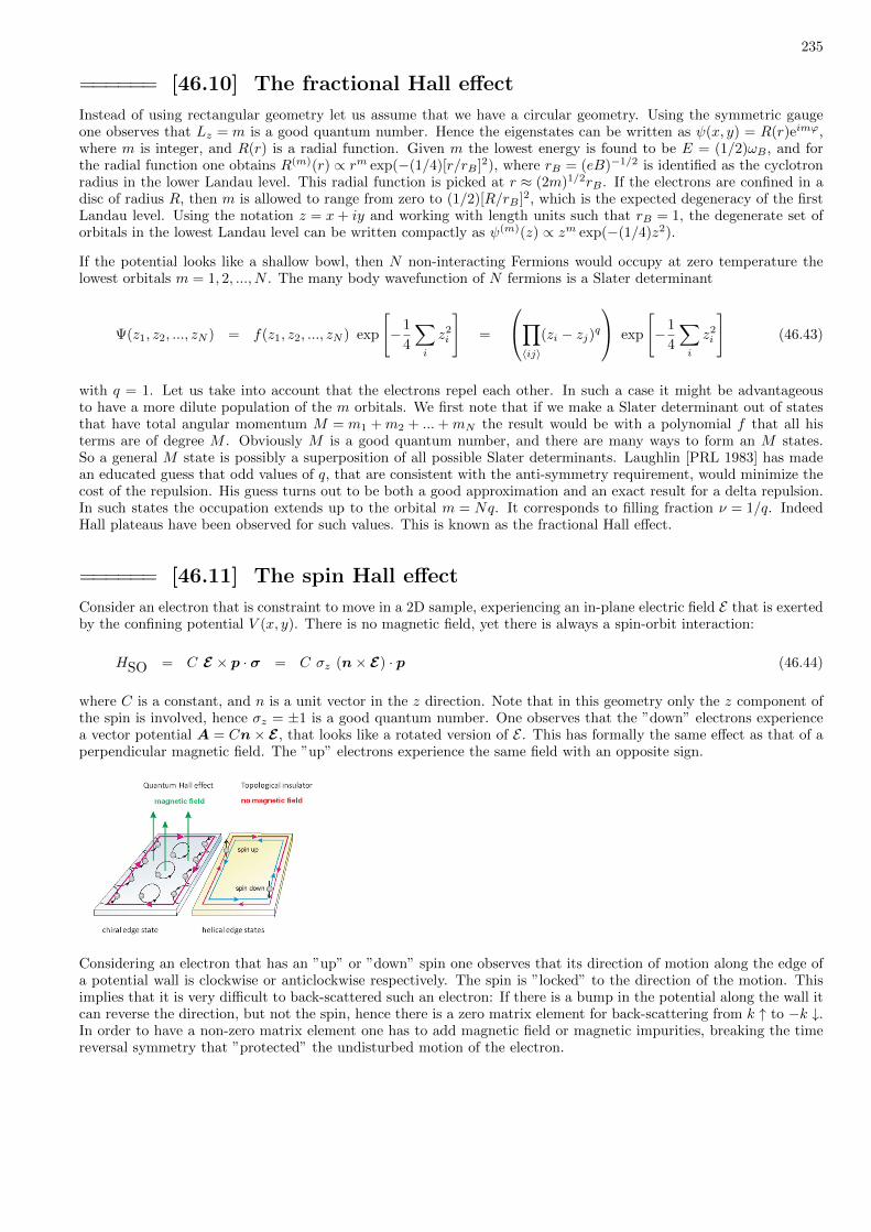
235

====== [46.10] The fractional Hall effect

Instead of using rectangular geometry let us assume that we have a circular geometry. Using the symmetric gaugeone observes that Lz = m is a good quantum number. Hence the eigenstates can be written as ψ(x, y) = R(r)eimϕ,where m is integer, and R(r) is a radial function. Given m the lowest energy is found to be E = (1/2)ωB , and forthe radial function one obtains R(m)(r) ∝ rm exp(−(1/4)[r/rB ]2), where rB = (eB)−1/2 is identified as the cyclotronradius in the lower Landau level. This radial function is picked at r ≈ (2m)1/2rB . If the electrons are confined in adisc of radius R, then m is allowed to range from zero to (1/2)[R/rB ]2, which is the expected degeneracy of the firstLandau level. Using the notation z = x+ iy and working with length units such that rB = 1, the degenerate set oforbitals in the lowest Landau level can be written compactly as ψ(m)(z) ∝ zm exp(−(1/4)z2).

If the potential looks like a shallow bowl, then N non-interacting Fermions would occupy at zero temperature thelowest orbitals m = 1, 2, ..., N . The many body wavefunction of N fermions is a Slater determinant

Ψ(z1, z2, ..., zN ) = f(z1, z2, ..., zN ) exp

[−1

4

∑i

z2i

]=

∏〈ij〉

(zi − zj)q exp

[−1

4

∑i

z2i

](46.43)

with q = 1. Let us take into account that the electrons repel each other. In such a case it might be advantageousto have a more dilute population of the m orbitals. We first note that if we make a Slater determinant out of statesthat have total angular momentum M = m1 +m2 + ...+mN the result would be with a polynomial f that all histerms are of degree M . Obviously M is a good quantum number, and there are many ways to form an M states.So a general M state is possibly a superposition of all possible Slater determinants. Laughlin [PRL 1983] has madean educated guess that odd values of q, that are consistent with the anti-symmetry requirement, would minimize thecost of the repulsion. His guess turns out to be both a good approximation and an exact result for a delta repulsion.In such states the occupation extends up to the orbital m = Nq. It corresponds to filling fraction ν = 1/q. IndeedHall plateaus have been observed for such values. This is known as the fractional Hall effect.

====== [46.11] The spin Hall effect

Consider an electron that is constraint to move in a 2D sample, experiencing an in-plane electric field E that is exertedby the confining potential V (x, y). There is no magnetic field, yet there is always a spin-orbit interaction:

HSO = C E × p · σ = C σz (n× E) · p (46.44)

where C is a constant, and n is a unit vector in the z direction. Note that in this geometry only the z component ofthe spin is involved, hence σz = ±1 is a good quantum number. One observes that the ”down” electrons experiencea vector potential A = Cn× E, that looks like a rotated version of E . This has formally the same effect as that of aperpendicular magnetic field. The ”up” electrons experience the same field with an opposite sign.

Considering an electron that has an ”up” or ”down” spin one observes that its direction of motion along the edge ofa potential wall is clockwise or anticlockwise respectively. The spin is ”locked” to the direction of the motion. Thisimplies that it is very difficult to back-scattered such an electron: If there is a bump in the potential along the wall itcan reverse the direction, but not the spin, hence there is a zero matrix element for back-scattering from k ↑ to −k ↓.In order to have a non-zero matrix element one has to add magnetic field or magnetic impurities, breaking the timereversal symmetry that ”protected” the undisturbed motion of the electron.

236

[47] Motion in a central potential

====== [47.1] The Hamiltonian

Consider the motion of a particle under the influence of a spherically symmetric potential that depends only on thedistance from the origin. We can write the Hamiltonian in “spherical coordinates” as a sum of radial term and an

additional azimuthal term that involves the generators ~L = ~r × ~p. Namely,

H =1

2mp2 + eV (r) =

1

2m

(p2r +

1

r2L2

)+ eV (r) (47.1)

In order to go form the first to the second expression we have used the vector style version of 1 = cos2 + sin2, whichis A2B2 = (A ·B)2 + (A×B)2, with A = r and B = p. One should be careful about operator ordering. Optionallywe can regard this identity as the differential representation of the Laplacian in spherical coordinates, with

p2r → −1

r

∂2

∂r2r (47.2)

The Hamiltonian commutes with rotations:

[H, R] = 0 (47.3)

And in particular:

[H, L2] = 0 (47.4)

[H, Lz] = 0

According to the separation of variables theorem the Hamiltonian becomes block diagonal in the basis whichis determined by L2 and Lz. The states that have definite ` and m quantum numbers are of the formψ(x, y, z) = R(r)Y `m(θ, ϕ), so there is some freedom in the choice of this basis. The natural choice is |r, `,m〉

〈r, θ, ϕ|r0, `0,m0〉 = Y `0,m0(θ, ϕ)1

rδ(r − r0) (47.5)

These are states that ”live” on spherical shells. Any wavefunction can be written as a linear combination of the statesof this basis. Note that the normalization is correct (the volume element in spherical coordinates includes r2). TheHamiltonian becomes

〈r, `,m|H|r′, `′,m′〉 = δ`,`′δm,m′H(`,m)r,r′ (47.6)

H(`,m) =1

2mp2 +

(`(`+ 1)

2mr2+ V (r)

)=

1

2mp2 + V (`)(r) (47.7)

where p→ −i(d/dr). The wavefunction in the basis which has been defined above are written as

|ψ〉 =∑r,`,m

u`m(r) |r, `,m〉 7−→∑`m

u`m(r)

rY `,m(θ, ϕ) (47.8)

In the derivation above we have made a ”shortcut”. In the approach which is popular in textbooks the basis is notproperly normalized, and the wave function is written as ψ(x, y, z) = ψ(r, θ, ϕ) = R(r)Y `,m(θ, ϕ), without taking thecorrect normalization measure into account. Only in a later stage they define u(r) = rR(r). Eventually they get thesame result. By using the right normalization of the basis we have saved an algebraic stage.

237

By separation of variables the Hamiltonian has been reduced to a semi-one-dimensional Schrodinger operator actingon the wave function u(r). By ”semi-one-dimensional” we mean that 0 < r <∞. In order to get a wave functionψ(x, y, z) that is continuous at the origin, we must require the radial function R(r) to be finite, or alternatively thefunction u(r) has to be zero at r = 0.

====== [47.2] Eigenstates of a particle on a spherical surface

The simplest central potential that we can consider is such that confine the particle to move within a spherical shellof radius R. Such potential can be modeled as V (r) = −λδ(r −R). For ` = 0 we know that a narrow deep well hasonly one bound state. We fix the energy of this state as the reference. The centrifugal potential for ` > 0 simply liftsthe potential floor upwards. Hence the eigen-energies are

E`m =1

2mR2`(`+ 1) (47.9)

We remind ourselves of the considerations leading to the degeneracies. The ground state Y 00, has the same symmetryas that of the Hamiltonian: both invariant under rotations. This state has no degeneracy. On the other hand, thestate Y 10 has a lower symmetry and by rotating it we get 3 orthogonal states with the same energy. The degeneracyis a ”compensation” for the low symmetry of the eigenstates: the symmetry of the energy level as a whole (i.e. as asubspace) is maintained.

The number of states N(E) up to energy E, that satisfy E`m < E, is easily found. The density of states turns out tobe constant:

dN

dE≈ m

2π~2A, A = 4πR2 (47.10)

It can be proved that this formula is valid also for other surfaces: to leading order only the surface area A is important.The most trivial example is obviously a square for which

En,m =π2

2mL2(n2 +m2) (47.11)

The difference between the E`m spectrum of a particle on a sphere, and the En,m spectrum of a particle on a square,is in the way that the eigenvalues are spaced, not in their average density. The degeneracies of the spectrum aredetermined by the symmetry group of the surface on which the motion is bounded. If this surface has no specialsymmetries the spectrum is expected to be lacking systematic degeneracies.

====== [47.3] The Hydrogen Atom

The effective potential V `(r) that appears in the semi-one-dimensional problem includes the original potential plusa centrifugal potential (for ` 6= 0). Typically, the centrifugal potential +1/r2 leads to the appearance of a potentialbarrier. Consequently there are ”resonance states” in the range E > 0, that can ”leak” out through the centrifugalbarrier (by tunnelling) into the outside continuum. But in the case of the Hydrogen atom the attractive potential−1/r wins over the centrifugal potential, and there is no such barrier. Moreover, unlike typical short range potentials,there are infinite number of bound states in the E < 0 range. Another special property of the Hydrogen atom isthe high degree of symmetry: the Hamiltonian commutes with the Runge-Lentz operators. This is manifested in thedegeneracy of energy levels, which is much greater than expected from SO(3).

For sake of later reference we write the potential as:

V (r) = −αcr, α =

e2

~c≈ 1

137(47.12)

238

Below we use as usual ~ = 1 units. Solving the radial equation (for each ` separately) one obtains:

E`,m,ν = [mc2] − α2mc2

2(`+ ν)2(47.13)

where ν = 1, 2, 3, . . .. The rest-mass of the atom has been added here in square brackets as a reminder that from arelativistic point of view we are dealing here with an expansion with respect to the fine structure constant α. In thenon-relativistic treatment this term is omitted. The energy levels are illustrated in the diagram below. It is customaryin text books to use the quantum number n = `+ ν in order to label the levels. One should bare in mind that the nquantum number has significance only for the 1/r potential due to its high symmetry: it has no meaning if we havesay 1/r5 potential.

0 1 2 3 4

−1

−0.8

−0.6

−0.4

−0.2

0

l

E lν

Degeneracies.– We would like to remind the reader why there are degeneracies in the energy spectrum (this issuehas been discussed in general in the section about symmetries and their implications). If the Hamiltonian has a singleconstant of motion, there will usually not be a degeneracy. According to the separation of variables theorem it ispossible to transform to a basis in which the Hamiltonian has a block structure, and then diagonalize each blockseparately. There is no reason for a conspiracy amongst the blocks. Therefore there is no reason for a degeneracy. Ifwe still get a degeneracy it is called an accidental degeneracy.

But, if the Hamiltonian commutes with a ”non-commutative group” then there are necessarily degeneracies that aredetermined by the dimensions of the irreducible representations. In the case of a central potential, the symmetrygroup is the ”rotation group”. In the special case of the potential −1/r a larger symmetry group exists.

A degeneracy is a compensation for having eigenstates with lower symmetry compared with the Hamiltonian. Thedegree of degeneracy is determined by the dimensions of the irreducible representations. These statements werediscussed in the Fundamentals II section. Let us paraphrase the argument in the present context: Assume that wehave found an eigenstate of the Hamiltonian. If it has full spherical symmetry then there is no reason for degeneracy.These are the states with ` = 0. But, if we have found a state with a lower symmetry (the states with ` 6= 0) then wecan rotate it and get another state with the same energy level. Therefore, in this case there must be a degeneracy.

Instead of ”rotating” an eigenstate, it is simpler (technically) to find other states with the same energy by using ladderoperators. This already gives an explanation why the degree of the degeneracy is determined by the dimension ofthe irreducible representations. Let us paraphrase the standard argument for this statements in the present context:The Hamiltonian H commutes with all the rotations, and therefore it also commutes with all their generators andalso with L2. We choose a basis |n, `, µ〉 in which both H and L2 are diagonal. The index of the energy levels n isdetermined by H, while the index ` is determined by L2. The index µ differentiates states with the same energy andthe same `. According to the ”separation of variables theorem” every rotation matrix will have a ”block structure” inthis basis: each level that is determined by the quantum numbers (n, `) is an invariant subspace under rotations. Inother words, H together with L2 induce a decomposition of the group representation. Now we can apply the standardprocedure in order to conclude that the dimension of the (sub) representation which is characterized by the quantumnumber `, is 2`+ 1. In other words, we have “discovered” that the degree of the degeneracy must be 2`+ 1 (or amultiple of this number).

239

Corrections.– The realistic expression for the energy levels of Hydrogen atom contains a term that originates fromthe relativistic Dirac equation, plus a Lamb-Shift due to the interaction with the fluctuations of the electromagneticvacuum, plus additional ”hyperfine” correction due to the interaction with the nucleus:

E`,j,m,ν = mc2

1 +

[α

ν + `− (j + s) +√

(j + s)2 − α2

]2−1/2

+ LambShift + HyperFine (47.14)

Disregarding the hyperfine interaction, the good quantum numbers are `, and j, and s = 1/2. Defining n = `+ ν andusing (n, `, j,m) as good quantum numbers, one observes that the eigen-energies are independent of `. It is customaryto expand the Dirac expression with respect to the the fine-structure constant α ≡ e2/(~c). The leading α2 term isthe same as that of Bohr. The next α4 term can be regarded as the sum of relativistic kinetic p4 correction, a Darwinterm δ3(r) that affects s-orbitals, and a spin-orbit term (1/r3)L·S. On top we have the α5 Lamb-shift correction, thatcan be approximated as an additional δ3(r) term. The Darwin and the Lamb-shift terms can be interpreted as arisingfrom the smearing of the 1/r interaction, either due to zitterbewegung or due to the fluctuations that are induced bythe electromagnetic field, respectively. The Lamb shift splits the degeneracy of the j = 1/2 levels ”2s” and ”2p”. TheLamb shift physics is also responsible for the anomalous value of the spin-orbit coupling (g ≈ 2 + (α/π)).

The spin-related fine-structure will be discussed in the next lectures. It will be regarded as arising from ”corrections”to the non-relativistic Schroedinger Hamiltonian. In particular we shall see how the quantum number j arises due tothe addition of the angular momentum of the spin, and the presence of the spin-orbit interaction.

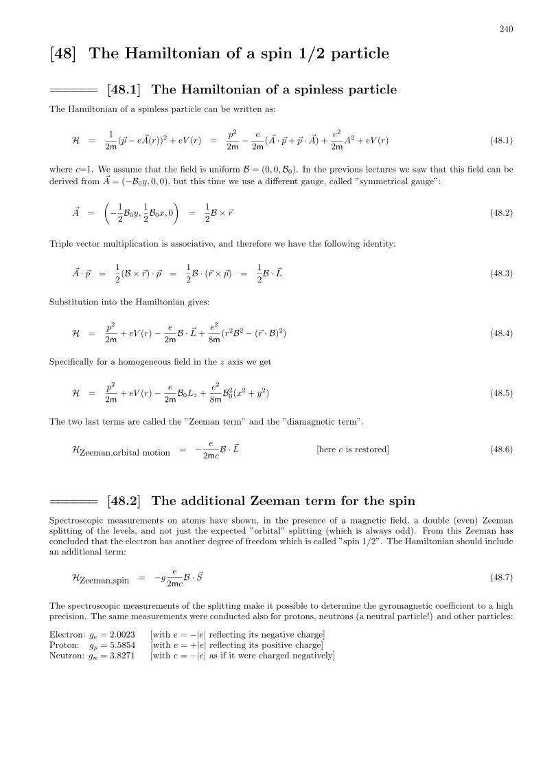
240

[48] The Hamiltonian of a spin 1/2 particle

====== [48.1] The Hamiltonian of a spinless particle

The Hamiltonian of a spinless particle can be written as:

H =1

2m(~p− e ~A(r))2 + eV (r) =

p2

2m− e

2m( ~A · ~p+ ~p · ~A) +

e2

2mA2 + eV (r) (48.1)

where c=1. We assume that the field is uniform B = (0, 0,B0). In the previous lectures we saw that this field can be

derived from ~A = (−B0y, 0, 0), but this time we use a different gauge, called ”symmetrical gauge”:

~A =

(−1

2B0y,

1

2B0x, 0

)=

1

2B × ~r (48.2)

Triple vector multiplication is associative, and therefore we have the following identity:

~A · ~p =1

2(B × ~r) · ~p =

1

2B · (~r × ~p) =

1

2B · ~L (48.3)

Substitution into the Hamiltonian gives:

H =p2

2m+ eV (r)− e

2mB · ~L+

e2

8m(r2B2 − (~r · B)2) (48.4)

Specifically for a homogeneous field in the z axis we get

H =p2

2m+ eV (r)− e

2mB0Lz +

e2

8mB2

0(x2 + y2) (48.5)

The two last terms are called the ”Zeeman term” and the ”diamagnetic term”.

HZeeman,orbital motion = − e

2mcB · ~L [here c is restored] (48.6)

====== [48.2] The additional Zeeman term for the spin

Spectroscopic measurements on atoms have shown, in the presence of a magnetic field, a double (even) Zeemansplitting of the levels, and not just the expected ”orbital” splitting (which is always odd). From this Zeeman hasconcluded that the electron has another degree of freedom which is called ”spin 1/2”. The Hamiltonian should includean additional term:

HZeeman,spin = −g e

2mcB · ~S (48.7)

The spectroscopic measurements of the splitting make it possible to determine the gyromagnetic coefficient to a highprecision. The same measurements were conducted also for protons, neutrons (a neutral particle!) and other particles:

Electron: ge = 2.0023 [with e = −|e| reflecting its negative charge]Proton: gp = 5.5854 [with e = +|e| reflecting its positive charge]Neutron: gn = 3.8271 [with e = −|e| as if it were charged negatively]

241

The implication of the Zeeman term in the Hamiltonian is that the wavefunction of the electron precesses with thefrequency

Ω = − e

2mcB (48.8)

while the spin of the electron precesses with a twice larger frequency

Ω = −gee

2mcB,

[ge ≈ 2

](48.9)

====== [48.3] The spin orbit term

The added Zeeman term describes the interaction of the spin with the magnetic field. In fact, the ”spin” degree offreedom (and the existence of anti-particles) is inevitable because of relativistic considerations of invariance underthe Lorentz transformation. These considerations lead to Dirac’s Hamiltonian. There are further ”corrections” tothe non-relativistic Hamiltonian that are required in order to make it ”closer” to Dirac’s Hamiltonian. The mostimportant of these corrections is the ”spin orbit interaction”:

Hspin−orbit = −(g−1)e

2(mc)2~E × ~p · ~S (48.10)

In other words, the spin interacts with the electric field. This interaction depends on its velocity. This is why theinteraction is called spin-orbit interaction. If there is also a magnetic field then we have the additional interactionwhich is described by the Zeeman term.

We can interpret the ”spin-orbit” interaction in the following way: even if there is no magnetic field in the ”laboratory”reference frame, still there is a magnetic field in the reference frame of the particle, which is a moving reference frame.This follows from Lorentz transformation:

B = B − (1/c)~vframe × E (48.11)

It looks by this argument that the spin-orbit term should be proportional to g, while in fact it is proportional to(g−1). The extra contribution is called “Thomas precession” and has a purely kinematical reason [discussed in thebook of Jackson]. The physical picture is as follows: the spin-orbit term originates from the component of the electricfield that is perpendicular to the velocity; This leads to a rotated motion; In the rotating rest-frame of the particle oneobserves precession due to the Zeeman interaction; Going back to the laboratory frame the Lorentz transformationimplies that the spin experiences an extra magnetic-like field, analogous to Coriolis. This is because the laboratoryframe is rotating with respect to the rest frame of the particle.

We summarize this section by writing the common non-relativistic approximation to the Hamiltonian of a particlewith spin 1/2.

H =1

2m

(~p− e

c~A(r)

)2

+ eV (r) − g e

2(mc)B · ~S − (g−1)

e

2(mc)2(E × ~p) · ~S (48.12)

In the case of spherically symmetric potential V (r) the electric field is

E = −V′(r)

r~r (48.13)

Consequently the Hamiltonian takes the form (here again c=1):

H =1

2m

(p2r +

1

r2L2

)+ eV (r) +

e2

8mB2r2⊥ −

e

2mB · ~L− g e

2mB · ~S + (g−1)

e

2m2

V ′(r)

r~L · ~S (48.14)

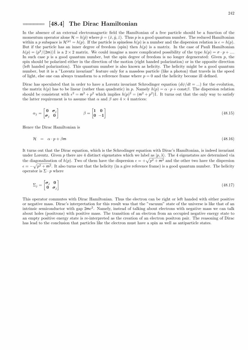
242

====== [48.4] The Dirac Hamiltonian

In the absence of an external electromagnetic field the Hamiltonian of a free particle should be a function of themomentum operator aloneH = h(p) where p = (x, y, z). Thus p is a good quantum number. The reduced Hamiltonianwithin a p subspace is H(p) = h(p). If the particle is spineless h(p) is a number and the dispersion relation is ε = h(p).But if the particle has an inner degree of freedom (spin) then h(p) is a matrix. In the case of Pauli Hamiltonian

h(p) = (p2/(2m))1 is a 2× 2 matrix. We could imagine a more complicated possibility of the type h(p) = σ · p+ ....In such case p is a good quantum number, but the spin degree of freedom is no longer degenerated: Given p, thespin should be polarized either in the direction of the motion (right handed polarization) or in the opposite direction(left handed polarization). This quantum number is also known as helicity. The helicity might be a good quantumnumber, but it is a ”Lorentz invariant” feature only for a massless particle (like a photon) that travels in the speedof light, else one can always transform to a reference frame where p = 0 and the helicity become ill defined.

Dirac has speculated that in order to have a Lorentz invariant Schrodinger equation (dψ/dt = ...) for the evolution,the matrix h(p) has to be linear (rather than quadratic) in p. Namely h(p) = α · p+ constβ. The dispersion relation

should be consistent with ε2 = m2 + p2 which implies h(p)2 = (m2 + p2)1. It turns out that the only way to satisfythe latter requirement is to assume that α and β are 4× 4 matrices:

αj =

[0 σjσj 0

]β =

[1 00 −1

](48.15)

Hence the Dirac Hamiltonian is

H = α · p+ βm (48.16)

It turns out that the Dirac equation, which is the Schrodinger equation with Dirac’s Hamiltonian, is indeed invariantunder Lorentz. Given p there are 4 distinct eigenstates which we label as |p, λ〉. The 4 eigenstates are determined via

the diagonalization of h(p). Two of them have the dispersion ε = +√p2 + m2 and the other two have the dispersion

ε = −√p2 + m2. It also turns out that the helicity (in a give reference frame) is a good quantum number. The helicity

operator is Σ · p where

Σj =

[σj 00 σj

](48.17)

This operator commutes with Dirac Hamiltonian. Thus the electron can be right or left handed with either positiveor negative mass. Dirac’s interpretation for this result was that the ”vacuum” state of the universe is like that of anintrinsic semiconductor with gap 2mc2. Namely, instead of talking about electrons with negative mass we can talkabout holes (positrons) with positive mass. The transition of an electron from an occupied negative energy state toan empty positive energy state is re-interpreted as the creation of an electron positron pair. The reasoning of Dirachas lead to the conclusion that particles like the electron must have a spin as well as antiparticle states.

243

[49] Implications of having ”spin”

====== [49.1] The Stern-Gerlach effect

We first discuss what effect the Zeeman term has on the dynamics of a ”free” particle. We shall see that because of thisterm, there is a force acting on the particle if the magnetic field is non-homogeneous. For simplicity of presentation weassume that the magnetic field is mainly in the Z direction, and neglect its other components. Defining r = (x, y, z)the Hamiltonian takes the form

H =~p2

2m− g e

2mBz(r)Sz (49.1)

We see that Sz is a constant of motion. If particle is prepared with spin ”up” it experiences an effective potential:

Veff = −1

2ge

2mBz(r) (49.2)

A a particle with spin ”down” experiences an inverted potential (with the opposite sign). That means that thedirection of the force depends on the direction of the spin. We can come to the same conclusion by looking at theequations of motion. The velocity of the particle is

d

dt〈r〉 = 〈i[H, r]〉 =

⟨1

m(~p−A(r))

⟩(49.3)

This still holds with no change. But what about the acceleration? We see that there is a new term:

d

dt〈v〉 = 〈i[H, v]〉 =

1

m

⟨Lorentz force + g

e

2m(∇Bz)Sz

⟩(49.4)

The observation that in inhomogeneous magnetic field the force on the particle depends on the spin orientation isused in order to measure the spin using a Stern-Gerlach apparatus.

====== [49.2] The reduced Hamiltonian in a central potential

We would like to consider the problem of electron in a central potential, say in the Hydrogen atom, taking into accountthe spin-orbit interaction. This add an L · S term to the Hamiltonian. We first would like to clarify what are thesurviving constants of motion. The system still has symmetry to rotations, and therefore the full Hamiltonian as wellas L · S commutes with J = L+ S. The Ji generate rotations of the wavefunction and the spin as one ”package”.The Hamiltonian does not commute with the generators Lx, Ly, Lz separately. For example [L · S,Lx] 6= 0. Stillthe Hamiltonian commutes with L2. In particular [L · S,L2] = 0. This is clear because L2 is a Casimir operators(commutes with all the generators). Note also that

~L · ~S =1

2

(J2 − L2 − S2

)(49.5)

Form the above we deduce that ` is still a good quantum number, and therefore it makes sense to work with theorbital states

|`mν〉 → R`ν(r)Y `m(θ, ϕ) (49.6)

The Hamiltonian in the ` subspace is

H(`) = H(`)0 −

e

2mBLz − g

e

2mBSz + f(r)L · S (49.7)

244

So far no approximations were involved. If we further assume that the last terms in the Hamiltonian is a weakperturbation that does not ”mix” energy levels, then we can make an approximation that reduces further Hamiltonianinto the subspace of states that have the same energy:

H(`ν) = −hLz − ghSz + vL · S + const (49.8)

where the first term with h = eB/(2m) is responsible for the orbital Zeeman splitting, and the second term with ghis responsible to the spin-related Zeeman splitting. Note that g = 2.0023. We also use the notation

v = 〈`, ν|f(r)|`, ν〉 (49.9)

If the spin-orbit interaction did not exist, the dynamics of the spin would become independent of the dynamics of thewave function. But even with the spin-orbit interaction, the situation is not so bad. L · S couples only states withthe same `. Furthermore the ` = 0 for which L · S = 0 are not affected by the spin-orbit interactions.

====== [49.3] The Zeeman Hamiltonian

From now we focus on the ` = 1 subspace in the second energy level of the Hydrogen atom. The Hamiltonian matrixis 6× 6. The reduced Hamiltonian can be written in the standard basis |` = 1, ν = 1,m`,ms〉. It is easy to write thematrices for the Zeeman terms:

Lz →

1 0 00 0 00 0 −1

⊗ (1 00 1

)=

1 0 0 0 0 00 1 0 0 0 00 0 0 0 0 00 0 0 0 0 00 0 0 0 −1 00 0 0 0 0 −1

(49.10)

Sz →

1 0 00 1 00 0 1

⊗ 1

2

(1 00 −1

)=

1

2

1 0 0 0 0 00 −1 0 0 0 00 0 1 0 0 00 0 0 −1 0 00 0 0 0 1 00 0 0 0 0 −1

But the spin-orbit term is not diagonal. The calculation of this term is more demanding:

~L · ~S =1

2

(J2 − L2 − S2

)=

1

2

(J2 − 11

4

)(49.11)

The calculation of the matrix that represent J2 in the standard basis is lengthy, though some shortcuts are possible(see lecture regarding ”addition of angular momentum”). Doing the calculation, the result for the total Hamiltonianis

H → −h

1 0 0 0 0 00 1 0 0 0 00 0 0 0 0 00 0 0 0 0 00 0 0 0 −1 00 0 0 0 0 −1

− gh

12 0 0 0 0 00 − 1

2 0 0 0 00 0 1

2 0 0 00 0 0 − 1

2 0 00 0 0 0 1

2 00 0 0 0 0 − 1

2

+ v

12 0 0 0 0 00 − 1

21√2

0 0 0

0 1√2

0 0 0 0

0 0 0 0 1√2

0

0 0 0 1√2− 1

2 0

0 0 0 0 0 12

(49.12)

At this stage we can diagonalize the Hamiltonian, and find exact results for the eigen-energies. However, we shall seein the next section that it is possible to find some shortcuts that save much of the technical burden.

245

====== [49.4] The Zeeman energies

We write again the Hamiltonian that we want to diagonalize:

H =v

2

(J2 − 11

4

)− hLz − ghSz (49.13)

There is a relatively simple way to figure out the representation of J2 using the ”addition theorem”. Namely, afterdiagonalization it should become:

J2 →

(15/4) 0 0 0 0 0

0 (15/4) 0 0 0 00 0 (15/4) 0 0 00 0 0 (15/4) 0 00 0 0 0 (3/4) 00 0 0 0 0 (3/4)

(49.14)

It follows that the exact eigenenergies of the Hamiltonian in the absence of a magnetic field are:

Ej= 32

= v/2, [degeneracy = 4] (49.15)

Ej= 12

= −v, [degeneracy = 2]

On the other hand, in a strong magnetic field the spin-orbit term is negligible, and we get:

Em`,ms ≈ −(m` + gms)h (49.16)

In fact there are two levels that are exact eigensates of the Hamiltonian for any h. These are:

Ej= 32 ,mj=±

32

=v

2∓(

1 +g

2

)h (49.17)

The spectrum of H can be found for a range of h values. See the Mathematica file zeeman.nb. The results (in unitssuch that v = 1) are illustrated in the following figure:

0 0.5 1 1.5 2 2.5 3

-2

-1

0

1

2

3

246

====== [49.5] Calculation of the Zeeman splitting

For a weak magnetic field it is better to write the Hamiltonian in the |j,mj〉 basis, so as to have ~L · ~S diagonal, whilethe Zeeman terms are treated as a perturbation. The calculation, using Mathematica, leads to

H → v

2

1 0 0 0 0 00 1 0 0 0 00 0 1 0 0 00 0 0 1 0 00 0 0 0 −2 00 0 0 0 0 −2

−h

3

3 0 0 0 0 0

0 1 0 0 −√

2 0

0 0 −1 0 0 −√

20 0 0 −3 0 0

0 −√

2 0 0 2 0

0 0 −√

2 0 0 −2

− gh

6

3 0 0 0 0 0

0 1 0 0 2√

2 0

0 0 −1 0 0 2√

20 0 0 −3 0 0

0 2√

2 0 0 −1 0

0 0 2√

2 0 0 1

Optionally, if we want to avoid the above numerical task, we can determine approximately the splitting of the jmultiplets using degenerate perturbation theory. In order to do so we only need to find the j sub-matrices of the theHamiltonian. We already know that they should obey the Wigner Eckart theorem. By inspection of the Hamiltonianwe see that this is indeed the case. We have gL = 2

3 and gS = 13 for j = 3

2 , while gL = 43 and gS = − 1

3 for j = 12 .

Hence we can write

Ej,mj = Ej − (gMmj)h (49.18)

where gM = gL + ggS is associated with the vector operator ~M = ~L+ g~S. In order to calculate gL and gS we do notneed to calculate the above 6× 6 matrices. We can simply can use the formulas

gL =〈 ~J · ~L〉j(j + 1)

=j(j + 1) + `(`+ 1)− s(s+ 1)

2j(j + 1)(49.19)

gS =〈 ~J · ~S〉j(j + 1)

=j(j + 1) + s(s+ 1)− `(`+ 1)

2j(j + 1)(49.20)

247

Special Topics

[50] Quantization of the EM Field

====== [50.1] The Classical Equations of Motion

The equations of motion for a system which is composed of non-relativistic classical particles and EM fields are:

mid2xidt2

= eiE − eiB × xi (50.1)

∇ · E = 4πρ

∇× E = −∂B∂t

∇ · B = 0

∇× B =∂E∂t

+ 4π ~J

where

ρ(x) =∑i

eiδ(x− xi) (50.2)

J(x) =∑i

eixiδ(x− xi)

We also note that there is a continuity equation which is implied by the above definition and also can be regarded asa consistency requirement for the Maxwell equation:

∂ρ

∂t= −∇ · J (50.3)

It is of course simpler to derive the EM field from a potential (V,A) as follows:

B = ∇×A (50.4)

E = −∂A∂t−∇V

Then we can write an equivalent system of equations of motion

mid2xidt2

= eiE − eiB × xi (50.5)

∂2A

∂t2= ∇2 ~A−∇

(∇ · ~A+

∂

∂tV

)+ 4πJ

∇2V = − ∂

∂t

(∇ · ~A

)− 4πρ

====== [50.2] The Coulomb Gauge

In order to further simplify the equations we would like to use a convenient gauge which is called the ”Coulomb gauge”.To fix a gauge is essentially like choosing a reference for the energy. Once we fix the gauge in a given reference frame(”laboratory”) the formalism is no longer manifestly Lorentz invariant. Still the treatment is exact.

248

Any vector field can be written as a sum of two components, one that has zero divergence and another that has zerocurl. For the case of the electric field E , the sum can be written as:

E = Eq + E⊥ (50.6)

where ∇ · E⊥ = 0 and ∇×Eq = 0. The field E⊥ is called the transverse or solenoidal or ”radiation” component, whilethe field Eq is the longitudinal or irrotational or ”Coulomb” component. The same treatment can be done for themagnetic field B with the observation that from Maxwell’s equations ∇ · B = 0 yields B‖ = 0. That means that thereis no magnetic charge and hence the magnetic field B is entirely transverse. So now we have

EM field = (Eq, E⊥,B) = Coulomb field + radiation field (50.7)

Without loss of generality we can derive the radiation field from a transverse vector potential. Thus we have:

Eq = −∇V (50.8)

E⊥ = −∂A∂t

B = ∇×A

This is called the Coulomb gauge, which we use from now on. We can solve the Maxwell equation for V in this gauge,leading to the potential

V (x) =∑j

ej|x− xj |

(50.9)

Now we can insert the solution into the equations of motion of the particles. The new system of equations is

mid2xidt2

=

∑j

eiej ~nij|xi − xj |2

+ eiE⊥ − eiB × xi (50.10)

∂2A

∂t2= ∇2 ~A+ 4πJ⊥

It looks as if Jq is missing in the last equation. In fact it can be easily shown that it cancells with the ∇V term dueto the continuity equation that relates ∂tρ to ∇ · J , and hence ∂t∇V to Jq respectively.

====== [50.3] Hamiltonian for the Particles

We already know from the course in classical mechanics that the Hamiltonian, from which the equations of motion ofone particles in EM field are derived, is

H(i) =1

2mi(pi − eiA(xi))

2 + eiV (xi) (50.11)

This Hamiltonian assumes the presence of A while V is potential which is created by all the other particles. Once weconsider the many body system, the potential V is replaced by a mutual Coulomb interaction term, from which theforces on any of the particles are derived:

H =∑i

1

2mi(pi − eiA(xi))

2 +1

2

∑i,j

eiej|xi − xj |

(50.12)

249

By itself the direct Coulomb interaction between the particles seems to contradict relativity. This is due to the non-invariant way that we had separated the electric field into components. In fact our treatment is exact: as a whole theHamiltonian that we got is Lorentz invariant, as far as the EM field is concerned.

The factor 1/2 in the Coulomb interaction is there in order to compensate for the double counting of the interactions.What about the diagonal terms i = j? We can keep them if we want because they add just a finite constant termto the Hamiltonian. The ”self interaction” infinite term can be regularized by assuming that each particle has a verysmall radius. To drop this constant from the Hamiltonian means that ”infinite distance” between the particles is takenas the reference state for the energy. However, it is more convenient to keep this infinite constant in the Hamiltonian,because then we can write:

H =∑i

1

2mi(pi − eiA(xi))

2 +1

8π

∫E2q d

3x (50.13)

In order to get the latter expression we have used the following identity:

1

2

∫ρ(x)ρ(x′)

|x− x′|d3xd3x′ =

1

8π

∫E2q d

3x (50.14)

The derivation of this identity is based on Gauss law, integration by parts, and using the fact that the Laplacian of1/|x− x′| is a delta function. Again we emphasize that the integral diverges unless we regularize the physical size ofthe particles, or else we have to subtract an infinite constant that represents the ”self interaction”.

====== [50.4] Hamiltonian for the Radiation Field

So now we need another term in the Hamiltonian from which the second equation of motion is derived

∂2A

∂t2−∇2 ~A = 4π ~J⊥ (50.15)

In order to decouple the above equations into ”normal modes” we write ~A in a Fourier series:

~A(x) =1√

volume

∑k

~Ak eikx =1√

volume

∑k,α

Ak,α εk,αeikx (50.16)

where εk,α for a given k is a set of two orthogonal unit vectors. If A were a general vector field rather than a transverse

field, then we would have to include a third unit vector. Note that ∇ · A = 0 is like k · ~Ak = 0. Now we can rewritethe equation of motion as

Ak,α + ω2kAk,α = 4πJk,α (50.17)

where ωk = |k|. The disadvantage of this Fourier expansion is that it does not reflect that A(x) is a real field. In factthe Ak,α should satisfy A−k,α = (Ak,α)∗. In order to have proper ”normal mode” coordinates we have to replace eachpair of complex Ak,α and A−k,α by a pair of real coordinates A′k,α and A′′k,α. Namely

Ak,α =1√2

[A′k,α + iA′′k,α] (50.18)

We also use a similar decomposition for Jk,α. We choose the 1/√

2 normalization so as to have the following identity:

∫J(x) ·A(x) dx =

∑k,α

J∗k,αAk,α =∑[k],α

(J ′k,αA′k,α + J ′′k,αA

′′k,α) ≡

∑r

JrQr (50.19)

250

In the sum over degrees of freedom r we must remember to avoid double counting. The vectors k and −k representthe same direction which we denote as [k]. The variable A′−k,α is the same variable as A′k,α, and the variable A′′−k,αis the same variable as −A′′k,α. We denote this set of coordinates Qr, and the conjugate momenta as Pr. We see that

each of the normal coordinates Qr has a ”mass” that equals 1/(4π) [CGS!!!]. Therefore the conjugate ”momenta” are

Pr = [1/(4π)]Qr, which up to a factor are just the Fourier components of the electric field. Now we can write theHamiltonian as

Hrad =∑r

[1

2 ·massP 2r +

1

2mass · ω2

r Q2r − JrQr

](50.20)

where r is the sum over all the degrees of freedom: two independent modes for each direction and polarization. Bystraightforward algebra the sum can be written as

Hrad =1

8π

∫(E2⊥ + B2)d3x−

∫~J ·Ad3x (50.21)

More generally, if we want to write the total Hamiltonian for the particle and the EM field we have to ensure that−∂H/∂A(x) = J(x). It is not difficult to figure out the the following Hamiltonian is doing the job:

H = Hparticles +Hinteraction +Hradiation =∑i

1

2mi(pi − eiA(xi))

2 +1

8π

∫(E2 + B2)d3x (50.22)

The term that corresponds to ~J ·A is present in the first term of the Hamiltonian. As expected this terms has a dualrole: on the one hand it gives the Lorentz force on the particle, while on the other hand it provides the source termthat drives the EM field. I should be emphasized that the way we write the Hamiltonian is somewhat misleading:The Coulomb potential term (which involves E2

q ) is combined with the ”kinetic” term of the radiation field (whichinvolves E2

⊥).

====== [50.5] Quantization of the EM Field

Now that we know the ”normal coordinates” of the EM field the quantization is trivial. For each ”oscillator” of ”mass”1/(4π) we can define a and a† operators such that Qr = (2π/ω)1/2(ar + a†r). Since we have two distinct variables foreach direction, we use the notations (b, b†) and (c, c†) respectively:

Q[k]′α = A′kα = A′−kα =

√2π

ωk

(b[k]α + b†[k]α

)(50.23)

Q[k]′′α = A′′kα = −A′′−kα =

√2π

ωk

(c[k]α + c†[k]α

)(50.24)

In order to make the final expressions look more elegant we use the following canonical transformation:

a+ =1√2

(b+ ic) (50.25)

a− =1√2

(b− ic)

It can be easily verified by calculating the commutators that the transformation from (b, c) to (a+, a−) is canonical.

Also note that b†b+ c†c = a†+a+ + a†−a−. Since the oscillators (normal modes) are uncoupled the total Hamiltonianis a simple sum over all the modes:

H =∑[k],α

(ωkb†k,αbk,α + ωkc

†k,αck,α) =

∑k,α

ωka†k,αak,α (50.26)

251

For completeness we also write the expression for the field operators:

Ak,α =1√2

(A′ + iA′′) =1√2

[√2π

ωk(b+ b†) + i

√2π

ωk(c+ c†)

]=

√2π

ωk(ak,α + a†−k,α) (50.27)

and hence

~A(x) =1√

volume

∑k,α

√2π

ωk(ak,α + a†−k,α) εk,αeikx (50.28)

The eigenstates of the EM field are

|n1, n2, n3, . . . , nk,α, . . . 〉 (50.29)

We refer to the ground state as the vacuum state:

|vacuum〉 = |0, 0, 0, 0, . . . 〉 (50.30)

Next we define the one photon state as follows:

|one photon state〉 = a†kα |vacuum〉 (50.31)

and we can also define two photon states (disregarding normalization):

|two photon state〉 = a†k2α2a†k1α1

|vacuum〉 (50.32)

In particular we can have two photons in the same mode:

|two photon state〉 = (a†k1α1)2 |vacuum〉 (50.33)

and in general we can have N photon states or any superposition of such states.

An important application of the above formalism is for the calculation of spontaneous emission. Let us assumethat the atom has an excited level EB and a ground state EA. The atom is prepared in the excited state, and theelectromagnetic field is assume to be initially in a vacuum state. According to Fermi Golden Rule the system decaysinto final states with one photon ωk = (EB − EA). Regarding the atom as a point-like object the interaction term is

Hinteraction ≈ −ecA(0) · v (50.34)

where v = p/m is the velocity operator. It is useful to realize that vAB = i(EB − EA)xAB . The vector ~D = xAB isknown as the dipole matrix element. It follows that matrix element for the decay is

|〈nkα = 1, A|Hinteraction|vacuum, B〉|2 =1

volume

(ec

)2

2πωk|εk,α ·D|2 (50.35)

In order to calculate the decay rate we have to multiply this expression by the density of the final states, to integrateover all the possible directions of k, and to sum over the two possible polarizations α.

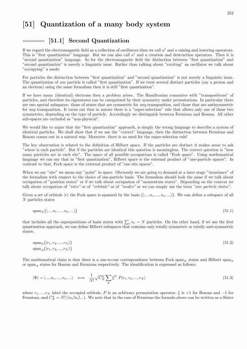
252

[51] Quantization of a many body system

====== [51.1] Second Quantization

If we regard the electromagnetic field as a collection of oscillators then we call a† and a raising and lowering operators.This is ”first quantization” language. But we can also call a† and a creation and destruction operators. Then it is”second quantization” language. So for the electromagnetic field the distinction between ”first quantization” and”second quantization” is merely a linguistic issue. Rather than talking about ”exciting” an oscillator we talk about”occupying” a mode.

For particles the distinction between ”first quantization” and ”second quantization” is not merely a linguistic issue.The quantization of one particle is called ”first quantization”. If we treat several distinct particles (say a proton andan electron) using the same formalism then it is still ”first quantization”.

If we have many (identical) electrons then a problem arises. The Hamiltonian commutes with ”transpositions” ofparticles, and therefore its eigenstates can be categorized by their symmetry under permutations. In particular thereare two special subspaces: those of states that are symmetric for any transposition, and those that are antisymmetricfor any transposition. It turns out that in nature there is a ”super-selection” rule that allows only one of these twosymmetries, depending on the type of particle. Accordingly we distinguish between Fermions and Bosons. All othersub-spaces are excluded as ”non-physical”.

We would like to argue that the ”first quantization” approach, is simply the wrong language to describe a system ofidentical particles. We shall show that if we use the ”correct” language, then the distinction between Fermions andBosons comes out in a natural way. Moreover, there is no need for the super-selection rule!

The key observation is related to the definition of Hilbert space. If the particles are distinct it makes sense to ask”where is each particle”. But if the particles are identical this question is meaningless. The correct question is ”howmany particles are in each site”. The space of all possible occupations is called ”Fock space”. Using mathematicallanguage we can say that in ”first quantization”, Hilbert space is the external product of ”one-particle spaces”. Incontrast to that, Fock space is the external product of ”one site spaces”.

When we say ”site” we mean any ”point” in space. Obviously we are going to demand at a later stage ”invariance” ofthe formalism with respect to the choice of one-particle basis. The formalism should look the same if we talk aboutoccupation of ”position states” or if we talk about occupation of ”momentum states”. Depending on the context wetalk about occupation of ”sites” or of ”orbitals” or of ”modes” or we can simply use the term ”one particle states”.

Given a set of orbitals |r〉 the Fock space is spanned by the basis |..., nr, ..., ns, ...〉. We can define a subspace of allN particles states

spanN|..., nr, ..., ns, ...〉 (51.1)

that includes all the superpositions of basis states with∑r nr = N particles. On the other hand, if we use the first

quantization approach, we can define Hilbert subspaces that contains only totally symmetric or totally anti-symmetricstates:

spanS|r1, r2, ..., rN 〉 (51.2)

spanA|r1, r2, ..., rN 〉

The mathematical claim is that there is a one-to-one correspondence between Fock spanN states and Hilbert spanSor spanA states for Bosons and Fermions respectively. The identification is expressed as follows:

|Ψ〉 = |..., nr, ..., ns, ...〉 ⇐⇒1

N !

√CnN

∑P

ξP P |r1, r2, ..., rN 〉 (51.3)

where r1, ..., rN label the occupied orbitals, P is an arbitrary permutation operator, ξ is +1 for Bosons and −1 forFermions, and CnN = N !/(nr!ns!...). We note that in the case of Fermions the formula above can be written as a Slater

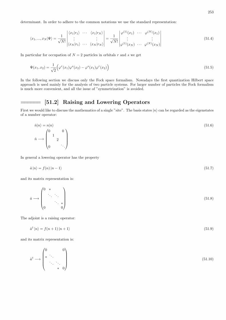
253

determinant. In order to adhere to the common notations we use the standard representation:

〈x1, ..., xN |Ψ〉 =1√N !

∣∣∣∣∣∣∣〈x1|r1〉 · · · 〈x1|rN 〉

......

〈xN |r1〉 · · · 〈xN |rN 〉

∣∣∣∣∣∣∣ =1√N !

∣∣∣∣∣∣∣ϕ(1)(x1) · · · ϕ(N)(x1)

......

ϕ(1)(xN ) · · · ϕ(N)(xN )

∣∣∣∣∣∣∣ (51.4)

In particular for occupation of N = 2 particles in orbitals r and s we get

Ψ(x1, x2) =1√2

(ϕr(x1)ϕs(x2)− ϕs(x1)ϕr(x2)

)(51.5)

In the following section we discuss only the Fock space formalism. Nowadays the first quantization Hilbert spaceapproach is used mainly for the analysis of two particle systems. For larger number of particles the Fock formalismis much more convenient, and all the issue of ”symmetrization” is avoided.

====== [51.2] Raising and Lowering Operators

First we would like to discuss the mathematics of a single ”site”. The basis states |n〉 can be regarded as the eigenstatesof a number operator:

n|n〉 = n|n〉 (51.6)

n −→

0 0

12

0. . .

In general a lowering operator has the property

a |n〉 = f(n) |n− 1〉 (51.7)

and its matrix representation is:

a −→

0 ∗

. . .. . .

. . . ∗0 0

(51.8)

The adjoint is a raising operator:

a† |n〉 = f(n+ 1) |n+ 1〉 (51.9)

and its matrix representation is:

a† −→

0 0

∗. . .

. . .. . .

∗ 0

(51.10)

254

By appropriate gauge we can assume without loss of generality that f(n) is real and non-negative. so we can write

f(n) =√g(n) (51.11)

From the definition of a it follows that

a†a|n〉 = g(n)|n〉 (51.12)

and therefore

a†a = g (n) (51.13)

There are 3 cases of interest

• The raising/lowering is unbounded (−∞ < n <∞)

• The raising/lowering is bounded from one side (say 0 ≤ n <∞)

• The raising/lowering is bounded from both sides (say 0 ≤ n < N )

The simplest choice for g(n) in the first case is

g(n) = 1 (51.14)

In such a case a becomes the translation operator, and the spectrum of n stretches from −∞ to ∞. The simplestchoice for g(n) in the second case is

g(n) = n (51.15)

this leads to the same algebra as in the case of an harmonic oscillator. The simplest choice for g(n) in the third caseis

g(n) = (N − n)n (51.16)

Here it turns out that the algebra is the same as that for angular momentum. To see that it is indeed like that define

m = n− N − 1

2= −s, . . . ,+s (51.17)

where s = (N − 1)/2. Then it is possible to write

g(m) = s(s+ 1)−m(m+ 1) (51.18)

In the next sections we are going to discuss the “Bosonic” case N = ∞ with g(n) = n, and the “Fermionic” caseN = 2 with g(n) = n(1 − n). Later we are going to argue that these are the only two possibilities that are relevantto the description of many body occupation.

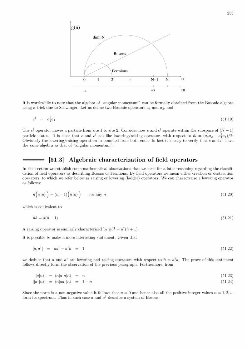
255

−s

0 1 2 N... n

m

dim=N

Fermions

+s

N−1

g(n)

Bosons

It is worthwhile to note that the algebra of “angular momentum” can be formally obtained from the Bosonic algebrausing a trick due to Schwinger. Let us define two Bosonic operators a1 and a2, and

c† = a†2a1 (51.19)

The c† operator moves a particle from site 1 to site 2. Consider how c and c† operate within the subspace of (N − 1)

particle states. It is clear that c and c† act like lowering/raising operators with respect to m = (a†2a2 − a†1a1)/2.Obviously the lowering/raising operation in bounded from both ends. In fact it is easy to verify that c and c† havethe same algebra as that of “angular momentum”.

====== [51.3] Algebraic characterization of field operators

In this section we establish some mathematical observations that we need for a later reasoning regarding the classifi-cation of field operators as describing Bosons or Fermions. By field operators we mean either creation or destructionoperators, to which we refer below as raising or lowering (ladder) operators. We can characterize a lowering operatoras follows:

n(a |n〉

)= (n− 1)

(a |n〉

)for any n (51.20)

which is equivalent to

na = a(n− 1) (51.21)

A raising operator is similarly characterized by na† = a†(n+ 1).

It is possible to make a more interesting statement. Given that

[a, a†] = aa† − a†a = 1 (51.22)

we deduce that a and a† are lowering and raising operators with respect to n = a†a. The prove of this statementfollows directly form the observation of the previous paragraph. Furthermore, from

||a|n〉|| = 〈n|a†a|n〉 = n (51.23)

||a†|n〉|| = 〈n|aa†|n〉 = 1 + n (51.24)

Since the norm is a non-negative value it follows that n = 0 and hence also all the positive integer values n = 1, 2, ...form its spectrum. Thus in such case a and a† describe a system of Bosons.

256

Let us now figure our the nature of an operator that satisfies the analogous anti-commutation relation:

[a, a†]+ = aa† + a†a = 1 (51.25)

Again we define n = a†a and observe that a and a† are characterized by na = a(1− n) and na† = a†(1− n). Hencewe deduce that both a and a† simply make transposition of two n states |ε〉 and |1−ε〉. Furthermore

||a|n〉|| = 〈n|a†a|n〉 = n (51.26)

||a†|n〉|| = 〈n|aa†|n〉 = 1− n (51.27)

Since the norm is a non-negative value it follows that 0 ≤ ε ≤ 1. Thus we deduce that the irreducible representationof a is

a =

(0

√ε√

1−ε 0

)(51.28)

One can easily verify the the desired anti-commutation is indeed satisfied. We can always re-define n such that n=0would correspond to one eigenvalue and n=1 would correspond to the second one. Hence it is clear that a and a†

describe a system of Fermions.

====== [51.4] Creation Operators for ”Bosons”

For a ”Bosonic” site we define

a |n〉 =√n |n− 1〉 (51.29)

hence

a† |n〉 =√n+ 1 |n+ 1〉 (51.30)

and

[a, a†

]= aa† − a†a = 1 (51.31)

If we have many sites then we define

a†r = 1⊗ 1⊗ · · · ⊗ a† ⊗ · · · ⊗ 1 (51.32)

which means

a†r |n1, n2, . . . , nr, . . . 〉 =√nr + 1 |n1, n2, . . . , nr + 1, . . . 〉 (51.33)

and hence

[ar, as] = 0 (51.34)

and

[ar, a

†s

]= δr,s (51.35)

257

We have defined our set of creation operators using a particular one-particle basis. What will happen if we switch toa different basis? Say from the position basis to the momentum basis? In the new basis we would like to have thesame type of ”occupation rules”, namely,

[aα, a

†β

]= δαβ (51.36)

Let’s see that indeed this is the case. The unitary transformation matrix from the original |r〉 basis to the new |α〉basis is

Tr,α = 〈r|α〉 (51.37)

Then we have the relation

|α〉 =∑r

|r〉 〈r|α〉 =∑r

Tr,α |r〉 (51.38)

and therefore

a†α =∑r

Tr,αa†r (51.39)

Taking the adjoint we also have

aα =∑r

T ∗r,αar (51.40)

Now we find that[aα, a

†β

]=∑r,s

[T ∗rαar, Tsβ a

†s

]= T ∗rαTsβδrs =

(T †)αrTrβ =

(T †T

)αβ

= δαβ (51.41)

This result shows that aα and a†β are indeed destruction and creation operators of the same ”type” as ar and a†r. Canwe have the same type of invariance for other types of occupation? We shall see that the only other possibility thatallows ”invariant” description is N = 2.

====== [51.5] Creation Operators for ”Fermions”

In analogy with the case of a ”Boson site” we define a ”Fermion site” using

a |n〉 =√n |n− 1〉 (51.42)

and

a† |n〉 =√n+ 1 |n+ 1〉 with mod(2) plus operation (51.43)

258

The representation of the operators is, using Pauli matrices:

n =

(1 00 0

)=

1

2

(1 + σ3

)(51.44)

a =

(0 01 0

)=

1

2(σ1 − iσ2)

a† =

(0 10 0

)=

1

2(σ1 + iσ2)

a†a = n

aa† = 1− n[a, a†

]+

= aa† + a†a = 1

while

[a, a†

]= 1− 2n (51.45)

Now we would like to proceed with the many-site system as in the case of ”Bosonic sites”. But the problem is thatthe algebra

[ar, a

†s

]= δr,s(1− 2a†rar) (51.46)

is manifestly not invariant under a change of one-particle basis. The only hope is to have

[ar, a

†s

]+

= δr,s (51.47)

which means that ar and as for r 6= s should anti-commute rather than commute. Can we define the operators ar insuch a way? It turns out that there is such a possibility:

a†r |n1, n2, . . . , nr, . . . 〉 = (−1)∑s(>r) ns

√1 + nr |n1, n2, . . . , nr + 1, . . . 〉 (51.48)

For example, it is easily verified that we have:

a†2a†1|0, 0, 0, . . . 〉 = −a†1a

†2|0, 0, 0, . . . 〉 = |1, 1, 0, . . . 〉 (51.49)

With the above convention if we create particles in the ”natural order” then the sign comes out plus, while for any”violation” of the natural order we get a minus factor.

====== [51.6] One Body Additive Operators

Let us assume that we have an additive quantity V which is not the same for different one-particle states. Oneexample is the (total) kinetic energy, another example is the (total) potential energy. It is natural to define the manybody operator that corresponds to such a property in the basis where the one-body operator is diagonal. In the caseof potential energy it is the position basis:

V =∑α

Vα,αnα =∑α

a†αVα,αaα (51.50)

This counts the amount of particles in each α and multiplies the result with the value of V at this site. If we go to a

259

different one-particle basis then we should use the transformation

aα =∑k

T ∗k,αak (51.51)

a†α =∑k′

Tk′,αa†k′

leading to

V =∑k,k‘

a†k′Vk′,kak (51.52)

Given the above result we can calculate the matrix elements from a transition between two different occupations:

|〈n1 − 1, n2 + 1|V |n1, n2〉|2 = (n2 + 1)n1 |V2,1|2 (51.53)

What we get is quite amazing: in the case of Bosons we get an amplification of the transition if the second level isalready occupied. In the case of Fermions we get ”blocking” if the second level is already occupied. Obviously thisgoes beyond classical reasoning. The latter would give merely n1 as a prefactor.

====== [51.7] Two Body “Additive” Operators

It is straightforward to make a generalization to the case of two body “additive” operators. Such operators mayrepresent the two-body interaction between the particles. For example we can take the Coulomb interaction, whichis diagonal in the position basis. Thus we have

U =1

2

∑α 6=β

Uαβ,αβnαnβ +1

2

∑α

Uαα,αα nα (nα − 1) (51.54)

Using the relation

a†αa†β aβ aα =

nαnβ for α 6= β

nα(nα − 1) for α = β(51.55)

We get the simple expression

U =1

2

∑α,β

a†αa†β Uαβ,αβ aβ aα (51.56)

and for a general one-particle basis

U =1

2

∑k′l′,kl

a†k′ a†l′ Uk′l′,kl alak (51.57)

We call such operator “additive” (with quotations) because in fact they are not really additive. An example fora genuine two body additive operator is [A,B], where A and B are one body operators. This observation is veryimportant in the theory of linear response (Kubo).

260

====== [51.8] Matrix elements with N particle states

Consider an N particle state of a Fermionic system, which is characterized by a definite occupation of k orbitals:

|RN 〉 = a†N . . . a†2a†1 |0〉 (51.58)

For the expectation value of a one body operator we get

〈RN |V |RN 〉 =∑k∈R

〈k|V |k〉 (51.59)

because only the terms with k = k′ do not vanish. If we have two N particle states with definite occupations, then thematrix element of V would be in general zero unless they differ by a single electronic transition, say from an orbitalk0 to another orbital k′0. In the latter case we get the result Vk′0,k0

as if the other electrons are not involved.

For the two body operator we get for the expectation value a more interesting result that goes beyond the naiveexpectation. The only non-vanishing terms in the sandwich calculation are those with either k′ = k and l′ = l or withk′ = l and l′ = k. All the other possibilities give zero. Consequently

〈RN |U |RN 〉 =1

2

∑k,l∈R

〈kl|U |kl〉direct

− 〈lk|U |kl〉exchange

(51.60)

A common application of this formula is in the context of multi-electron atoms and molecules, where U is theCoulomb interaction. The direct term has an obvious electrostatic interpretation, while the exchange term reflects theimplications of the Fermi statistics. In such application the exchange term is non-vanishing whenever two orbitals havea non-zero spatial overlap. Electrons that occupy well separated orbitals have only a direct electrostatic interaction.

====== [51.9] Introduction to the Kondo problem

One can wonder whether the Fermi energy, due to the Pauli exclusion principle, is like a lower cutoff that “regularize”the scattering cross section of of electrons in a metal. We explain below that this is not the case unless the scatteringinvolves a spin flip. The latter is known as the Kondo effect. The scattering is described by

V =∑k′,k

a†k′Vk′,kak (51.61)

hence:

T [2] =

⟨k2

∣∣∣∣V 1

E −H+ i0V

∣∣∣∣ k1

⟩=

∑k′b,kb

∑k′a,ka

⟨k2

∣∣∣∣a†k′bVk′b,kbakb 1

E −H+ i0a†k′a

Vk′a,kaaka

∣∣∣∣ k1

⟩(51.62)

where both the initial and the final states are zero temperature Fermi sea with one additional electron above theFermi energy. The initial and final states have the same energy:

E = E0 + εk1= E0 + εk2

(51.63)

where E0 is the total energy of the zero temperature Fermi sea. The key observation is that all the intermediatestates are with definite occupation. Therefore we can pull out the resolvent:

T [2] =∑

k′b,kb,k′a,ka

Vk′b,kbVk′a,kaE − Eka,k′a

⟨k2

∣∣∣a†k′bakba†k′aaka ∣∣∣ k1

⟩(51.64)

261

where

Eka,k′a = E0 + εk1− εka + εk′a (51.65)

time

k = represeneted by directionk = represeneted by vertical shift

Energy levels diagram Feynman diagram

As in the calculation of “exchange” we have two non-zero contribution to the sum. These are illustrated in the figureabove: Either (k′b, kb, k

′a, ka) equals (k2, k

′, k′, k1) with k′ above the Fermi energy, or (k′, k1, k2, k′) with k′ below the

Fermi energy. Accordingly E − Eka,k′a equals either (εk1− εk′) or −(εk1

− εk′). Hence we get

T [2] =∑k′

[Vk2,k′Vk′,k1

+(εk1 − εk′) + i0

⟨k2

∣∣∣a†k2ak′a

†k′ak1

∣∣∣ k1

⟩+

Vk′,k1Vk2,k′

−(εk1 − εk′) + i0

⟨k2

∣∣∣a†k′ak1a†k2ak′∣∣∣ k1

⟩](51.66)

Next we use⟨k2

∣∣∣a†k2ak′a

†k′ak1

∣∣∣ k1

⟩=⟨k2

∣∣∣a†k2(1− nk′)ak1

∣∣∣ k1

⟩= +1×

⟨k2

∣∣∣a†k2ak1

∣∣∣ k1

⟩(51.67)

which holds if k′ is above the Fermi energy (otherwise it is zero). And⟨k2

∣∣∣a†k′ak1a†k2

ak′∣∣∣ k1

⟩=⟨k2

∣∣∣ak1(nk′)a

†k2

∣∣∣ k1

⟩= −1×

⟨k2

∣∣∣a†k2ak1

∣∣∣ k1

⟩(51.68)

which holds if k′ is below the Fermi energy (otherwise it is zero). Note that without loss of generality we can assume

gauge such that 〈k2|a†k2ak1 |k1〉 = 1. Coming back to the transition matrix we get a result which is not divergent at

the Fermi energy:

T [2] =∑

k′∈above

Vk2,k′Vk′,k1

εk1− εk′ + i0

+∑

k′∈below

Vk2,k′Vk′,k1

εk1− εk′ − i0

(51.69)

If we are above the Fermi energy, then it is as if the Fermi energy does not exist at all. But if the scattering involvesa spin flip, as in the Kondo problem, the divergence for ε close to the Fermi energy is not avoided. Say that we wantto calculate the scattering amplitude

〈k2 ↑,⇓ |T | k1, ↑,⇓〉 (51.70)

where the double arrow stands for the spin of a magnetic impurity. It is clear that the only sequences that contributeare those that take place above the Fermi energy. The other set of sequences, that involve the creation of an electron-hole pair do not exist: Since we assume that the magnetic impurity is initially ”down”, it is not possible to generatea pair such that the electron spin is ”up”.

262

====== [51.10] Green functions for many body systems

The Green function in the one particle formalism is defined via the resolvent as the Fourier transform of the propagator.In the many body formalism the role of the propagator is taken by the time ordered correlation of field operators.In both cases the properly defined Green function can be used in order to analyze scattering problems in essentiallythe same manner. It is simplest to illustrate this observation using the example of the previous section. The Greenfunction in the many body context is defined as

Gk2,k1(ε) = −iFT[⟨

Ψ∣∣T ak2(t2)a†k1

(t1)∣∣Ψ⟩] (51.71)

If Ψ is the vacuum state this coincides with the one particle definition of the Green function:

Gk2,k1(ε) = −iFT

[Θ(t2−t1)

⟨k2|U(t2 − t1)|k1〉

](51.72)

But if Ψ is (say) a non-empty zero temperature Fermi sea then also for t2 < t1 we get a non-zero contribution due tothe possibility to annihilate an electron in an occupied orbital. Thus we get

Gk2,k1(ε) =

∑εk>εF

δk1,kδk2,k

ε− εk + i0+∑εk<εF

δk1,kδk2,k

ε− εk − i0(51.73)

One should observe that the many-body definition is designed so as to reproduce the correct T matrix as found inthe previous section. The definition above allows us to adopt an optional point of view of the scattering process: aone particle point of view instead of a many body point of view! In the many body point of view an electron-hole paircan be created, and later the hole is likely to be annihilated with the injected electron. In the one particle point ofview the injected electron can be “reflected” to move backwards in time and then is likely to be scattered back to theforward time direction. The idea here is to regard antiparticles as particles that travel backwards in time. This ideais best familiar in the context of the Dirac equation.

263

[52] Wigner function and Wigner-Weyl formalism

====== [52.1] The classical description of a state

Classical states are described by a probability function. Given a random variable x, we define ρ(x) = Prob(x = x) asthe probability of the event x = x, where the possible values of x are called the spectrum of the random variable x. Fora random variable continuous spectrum we define the probability density function via ρ(x)dx = Prob(x < x < x+ dx).

The expectation value of a random variable A = A(x) is defined as

〈A〉 =∑

ρ(x) A(x) (52.1)

and for a continuous variable as. For simplicity we use, from now on, a notation as if the random variables have adiscrete spectrum, with the understanding that in the case of a continuous spectrum we should replace the

∑by an

integral with the appropriate measure (e.g. dx or dp/(2π~)). Unless essential for the presentation we set ~ = 1.

Let us consider two random variables x, p. One can ask what is the joint probability distribution for these twovariables. This is a valid question only in classical mechanics. In quantum mechanics one usually cannot ask thisquestion since not all variables can be measured in the same measurement. In order to find the joint probabilityfunction of these two variables in quantum mechanics one needs to build a more sophisticated method. The solutionis to regard the expectation value as the fundamental outcome and to define the probability function as an expectationvalue. In the case of one variable such as x or p, we define probability functions as

ρ(X) ≡ 〈 δ(x−X) 〉 (52.2)

ρ(P ) ≡ 〈 2πδ(p− P ) 〉

Now we can also define the joint probability function as

ρ(X,P ) = 〈2πδ(p− P ) δ(x−X) 〉 (52.3)

This probability function is normalized so that∫ρ(X,P )

dXdP

2π=

⟨∫δ(p− P )dP

∫δ(x−X)dX

⟩= 1 (52.4)

In the next section we shall define essentially the same object in the framework of quantum mechanics.

====== [52.2] Wigner function

Wigner function is a real normalized function which is defined as

ρW(X,P ) =⟨ [

2πδ(p− P ) δ(x−X)]

sym

⟩(52.5)

In what follows we define what we mean by symmetrization (“sym”), and we relate ρW(X,P ) to the conventionalprobability matrix ρ(x′, x′′). We recall that the latter is defined as

ρ(x′, x′′) =⟨P x′x′′⟩

=⟨|x′′〉〈x′|

⟩(52.6)

The “Wigner function formula” that we are going to prove is

ρW(X,P ) =

∫ρ

(X +

1

2r,X − 1

2r

)e−iPrdr (52.7)

264

Thus to go from the probability matrix to the Wigner function is merely a Fourier transform, and can be looselyregarded as a change from “position representation” to “phase space representation”.

Moreover we can use the same transformation to switch the representation of an observable A from A(x′, x′′) toA(X,P ) . Then we shall prove the “Wigner-Weyl formula”

trace(Aρ) =

∫A(X,P )ρW(X,P )

dXdP

2π(52.8)

This formula implies that expectation values of an observable can be calculated using a semi-classical calculation.This extension of the Wigner function formalism is known as the Wigner-Weyl formalism.

====== [52.3] Mathematical derivations

Fourier transform reminder:

F (k) =

∫f(x)e−ikxdx (52.9)

f(x) =

∫dk

2πF (k)eikx

The inner product is invariant under change of representation∫f∗(x)g(x)dx =

∫dk

2πF ∗(k)G(k) (52.10)

For the matrix representation of an operator A we use the notation

A(x′, x′′) = 〈x′|A|x′′〉 (52.11)

It is convenient to replace the row and column indexes by diagonal and off-diagonal coordinates:

X =1

2(x′ + x′′) = the diagonal coordinate (52.12)

r = x′ − x′′ = the off diagonal coordinate

such that x′ = X + (r/2) and x′′ = X − (r/2), and to use the alternate notation

A(X, r) =

⟨X +

1

2r∣∣∣A∣∣∣X − 1

2r

⟩(52.13)

Using this notation, the transformation to phase space representations can be written as

A(X,P ) =

∫A(X, r)e−iPrdr (52.14)

Consequently the inner product of two matrices can be written as a phase space integral

trace(A†B) =

∫A∗(x′, x′′)B(x′, x′′)dx′dx′′ =

∫A∗(X, r)B(X, r)dXdr =

∫A∗(X,P )B(X,P )

dXdP

2π(52.15)

This we call the ”Wigner-Weyl formula”. Note that if A is hermitian then A(X,−r) = A∗(X,+r), and consequentlyA(X,P ) is a real function.

265

For the derivation of the “Wigner function formula” we have to explain how the operators δ(p− P )δ(x−X) aresymmetrized, and that that they form a complete set of observables that are linearly related to the standard set|x′〉〈x′′|. First we recall that a projector can be written as a delta function. This is quite transparent in discretenotation, namely |n0〉〈n0| = δn,n0 . The left hand side is a projector whose only non-zero matrix element is n = m = n0.The right hand side is a function of f(n) such that f(n) = 1 for n = n0 and zero otherwise. Therefore the right handside is also diagonal in n with the same representation. In continuum notation

|X〉〈X| = δ(x−X) =

∫dp

2πeip(x−X) (52.16)

With the same spirit we define the symmetrized operator

[2πδ(p− P ) δ(x−X)

]sym

≡∫drdp

2πeir(p−P )+ip(x−X) =

∫dre−irP

∫dp

2πeirp+ip(x−X) (52.17)

The inner integral can be carried out:∫dp

2πeirp+ip(x−X) =

∫dp

2πei(r/2)peip(x−X)ei(r/2)p = ei(r/2)pδ(x−X)ei(r/2)p (52.18)

where we used the identity eA+B = eAeBe12 [A,B], and the commutation [x, p] = i, in order to split the exponents, as

in the equality ex+p = ep/2exep/2. Replacing the δ(x−X) by |X〉〈X|, and operating on the ket and on the bra withthe displacement operators e±i(r/2)p we find that

[2πδ(p− P ) δ(x−X)

]sym

=

∫dre−irP

∣∣∣X−(r/2)⟩⟨X+(r/2)

∣∣∣ (52.19)

Taking the trace of both sides with ρ we deduce that ρW(X,P ) is related to ρ(X, r) via a Fourier transform in ther variable.

====== [52.4] Applications of the Wigner Weyl formalism

In analogy with the definition of the Wigner function ρW(X,P ) which is associated with ρ we can define a Wigner-

Weyl representation AWW(X,P ) of any hermitian operator A. The phase space function AWW(X,P ) is obtained fromthe standard representation A(x′, x′′) using the same “Wigner function formula” recipe. Let us consider the simplestexamples. First consider how the recipe works for the operator x:

〈 x′|x|x′′〉 = x′δ(x′ − x′′) = Xδ(r)WW7−→ X (52.20)

Similarly pWW→ P . Further examples are:

f(x)WW7−→ f(X) (52.21)

g(p)WW7−→ g(P ) (52.22)

xpWW7−→ XP +

1

2i (52.23)

pxWW7−→ XP − 1

2i (52.24)

1

2(xp+ px)

WW7−→ XP (52.25)

In general for appropriate ordering we get that f(x, p) is represented by f(X,P ). But in practical applications f(x, p)will not have the desired ordering, and therefore this recipe should be considered as a leading term in a semiclassical~ expansion.

266

There are two major applications of the Wigner Weyl formula. The first one is the calculation of the partition function.

Z(β) =∑r

e−βEr =∑r

⟨r|e−βH |r

⟩= trace(e−βH) =

∫dXdP

2π(e−βH(X,P )) +O(~) (52.26)

The second one is the calculation of the number of eigenstates up to a given energy E

N (E) =∑Er≤E

1 =∑r

Θ(E − Er) = trace[Θ(E − H)] (52.27)

≈∫dXdP

2πΘ(E −H(X,P )) =

∫H(X,P )≤E

dXdP

2π

Below we discuss some further applications that shed light on the dynamics of wavepackets, interference, and on thenature of quantum mechanical states. We note that the time evolution of Wigner function is similar but not identicalto the evolution of a classical distribution unless the Hamiltonian is a quadratic function of x and p.

====== [52.5] Wigner function for a Gaussian wavepacket

A Gaussian wavepacket in the position representation is written as

Ψ(x) =1√√2πσ

e−(x−x0)2

4σ2 eip0x (52.28)

The probability density matrix is

ρ(X, r) = Ψ

(X+

1

2r

)Ψ∗(X−1

2r

)(52.29)

=1√2πσ

e−((X−x0)+ 1

2r)2

4σ2 −((X−x0)− 1

2r)2

4σ2 +ip0r =1√2πσ

e−(X−x0)2

2σ2 − r2

8σ2 +ip0r

Transforming to the Wigner representation

ρW(X,P ) =

∫1√2πσ

e−(X−x0)2

2σ2 − r2

8σ2−i(P−p0)rdr =1

σxσpe− (X−x0)2

2σ2x− (P−p0)2

2σ2p (52.30)

where σx = σ and σp = 12σ . It follows that σxσp = 1/2. Let us no go backwards. Assume that have a Gaussian in

phase space, which is characterized by some σx and σp. Does it represent a legitimate quantum mechanical state?The normalization condition trace(ρ) = 1 is automatically satisfied. We also easily find that

trace(ρ2) =

∫1

σ2xσ

2p

e− (X−x0)2

σ2x− (P−p0)2

σ2p

dXdP

2π=

1

2σxσp(52.31)

We know that trace(ρ2) = 1 implies pure state. If trace(ρ2) < 1 it follows that we have a mixed state, whereastrace(ρ2) > 1 is not physical. It is important to remember that not any ρ(X,P ) corresponds to a legitimate quantummechanical state. There are classical states that do not have quantum mechanical analog (e.g. point like preparation).Also the reverse is true: not any quantum state has a classical analogue. The latter is implied by the possibility tohave negative regions in phase space. These is discussed in the next example.

267

====== [52.6] The Winger function of a bounded particle

Wigner function may have some modulation on a fine scale due to an interference effect. The simplest and mostilluminating example is the Wigner function of the nth eigenstate of a particle in a one dimensional box (0 < x < L).The eigen-wavefunction that correspond to wavenumber k = (π/L)× integer can be written as the sum of a right

moving and a left moving wave ψ(x) = (1/√

2)(ψ1(x) + ψ2(x)) within 0 < x < L, and ψ(x) = 0 otherwise. Thecorresponding Wigner function is zero outside of the box. Inside the box it can be written as

ρW(X,P ) =1

2ρ1(X,P ) +

1

2ρ2(X,P ) + ρ12(X,P ) (52.32)

where ρ12 is the interference component. The semiclassical components are concentrated at P = ±k, while theinterference component is concentrated at P = 0. The calculation of ρ1(X,P ) in the interval 0 < x < L/2 isdetermined solely by the presence of the hard wall at x = 0. The relevant component of the wavefunction is

ψ1(x) =1√L

Θ(x)eikx (52.33)

and hence

ρ1(X,P ) =

∫ ∞−∞

ψ1(X + (r/2))ψ∗1(X − (r/2))e−iPrdr =1

L

∫ ∞−∞

Θ(X + (r/2))Θ(X − (r/2))e−i(P−k)rdr

=1

L

∫ 2X

−2X

e−i(P−k)rdr =4X

Lsinc(2X(P − k)) (52.34)

This shows that as we approach the sharp feature the non-classical nature of Wigner function is enhanced, and theclassical (delta) approximation becomes worse. The other components of Wigner function are similarly calculated,and for the interference component we get

ρ12(X,P ) = −2 cos(2kX)× 4X

Lsinc(2XP ) (52.35)

It is easily verified that integration of ρW(X,P ) over P gives ρ(x) = 1 + 1− 2 cos(2kX) = 2(sin(kX))2.

In many other cases the energy surface in phase space is “soft” (no hard walls) and then one can derive a uniformsemiclassical approximation [Berry, Balazs]:

ρW(X,P ) =2π

∆sc(X,P )Ai

(H(X,P )− E

∆sc(X,P )

)(52.36)

where for H = p2/(2m) + V (x)

∆sc =1

2

[~2

(1

m|∇V (X)|2 +

1

m2(P · ∇)2V (X)

)]1/3

(52.37)

What can we get out of this expression? We see that ρW(X,P ) decays exponentially as we go outside of the energysurface. Inside the energy surface we have oscillations due to interference.

The interference regions of the Wigner function might be very significant. A nice example is given by Zurek. Letus assume that we have a superposition of N 1 non-overlapping Gaussian. we can write the Wigner function asρ = (1/N)

∑ρj + ρintrfr. We have trace(ρ) = 1 and also trace(ρ2) = 1. This implies that trace(ρintrfr) = 0, while

trace(ρ2intrfr) ∼ 1. The latter conclusion stems from the observation that the classical contribution is N × (1/N)2 1.

Thus the interference regions of the Wigner function dominate the calculation.

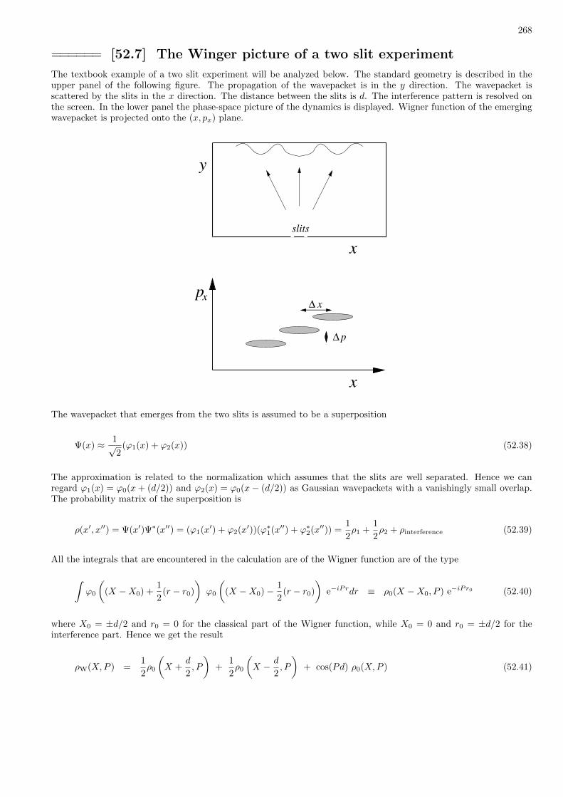
268

====== [52.7] The Winger picture of a two slit experiment

The textbook example of a two slit experiment will be analyzed below. The standard geometry is described in theupper panel of the following figure. The propagation of the wavepacket is in the y direction. The wavepacket isscattered by the slits in the x direction. The distance between the slits is d. The interference pattern is resolved onthe screen. In the lower panel the phase-space picture of the dynamics is displayed. Wigner function of the emergingwavepacket is projected onto the (x, px) plane.

slits

x

p

∆

∆

x

x

px

y

The wavepacket that emerges from the two slits is assumed to be a superposition

Ψ(x) ≈ 1√2

(ϕ1(x) + ϕ2(x)) (52.38)

The approximation is related to the normalization which assumes that the slits are well separated. Hence we canregard ϕ1(x) = ϕ0(x+ (d/2)) and ϕ2(x) = ϕ0(x− (d/2)) as Gaussian wavepackets with a vanishingly small overlap.The probability matrix of the superposition is

ρ(x′, x′′) = Ψ(x′)Ψ∗(x′′) = (ϕ1(x′) + ϕ2(x′))(ϕ∗1(x′′) + ϕ∗2(x′′)) =1

2ρ1 +

1

2ρ2 + ρinterference (52.39)

All the integrals that are encountered in the calculation are of the Wigner function are of the type

∫ϕ0

((X −X0) +

1

2(r − r0)

)ϕ0

((X −X0)− 1

2(r − r0)

)e−iPrdr ≡ ρ0(X −X0, P ) e−iPr0 (52.40)

where X0 = ±d/2 and r0 = 0 for the classical part of the Wigner function, while X0 = 0 and r0 = ±d/2 for theinterference part. Hence we get the result

ρW(X,P ) =1

2ρ0

(X +

d

2, P

)+

1

2ρ0

(X − d

2, P

)+ cos(Pd) ρ0(X,P ) (52.41)

269

Note that the momentum distribution can be obtained by integrating over X

ρ(P ) = (1 + cos(Pd))ρ0(P ) = 2 cos2(Pd

2)ρ0(P ) (52.42)

In order to analyze the dynamics it is suggestive to write ρ(X,P ) schematically as a sum of partial-wavepackets, eachcharacterized by a different transverse momentum:

ρW(X,P ) =

∞∑n=−∞

ρn(X,P ) (52.43)

By definition the partial-wavepacket ρn equals ρ for |P − n × (2π~/d)| < π~/d and equals zero otherwise. Eachpartial wavepacket represents the possibility that the particle, being scattered by the slits, had acquired a transversemomentum which is an integer multiple of

∆p =2π~d

(52.44)

The corresponding angular separation is

∆θ =∆p

P=

λBd

(52.45)

as expected. The associated spatial separation if we have a distance y from the slits to the screen is ∆x = ∆θy. It isimportant to distinguish between the “preparation” zone y < d, and the far-field (Franhaufer) zone y d2/λB . Inthe latter zone we have ∆x d or equivalently ∆x∆p 2π~.

====== [52.8] Thermal states

A stationary state ∂ρ/∂t has to satisfy [H, ρ] = 0. This means that ρ is diagonal in the energy representation. It canbe further argued that in typical circumstances the thermalized mixture is of the canonical type. Namely

ρ =∑|r〉pr〈r| =

1

Z∑|r〉e−βEr 〈r| = 1

Ze−βH (52.46)

Let us consider some typical examples. The first example is spin 1/2 in a magnetic field. In this case the energies areE↑ = ε/2 and E↓ = ε/2. Therefore ρ takes the following form:

ρ =1

2 cosh( 12βε)

(eβ

ε2 0

0 e−βε2

)(52.47)

Optionally one can represent the state of the spin by the polarization vector

~M =(

0, 0, tanh(1

2βε))

(52.48)

The next example is a free particle. The Hamiltonian is H = p2/2m. The partition function is

Z =

∫dk

(2π)/Le−β

k2

2m =

∫dXdP

2πe−β

P2

2m = L

(m

2πβ

) 12

(52.49)

270

The probability matrix ρ is diagonal in the p representation, and its Wigner function representation is identicalwith the classical expression. The standard x representation can be calculated either directly or via inverse Fouriertransform of the Wigner function:

ρ(x′, x′′) =

(1

L

)e−

m2β [x′−x′′]2 (52.50)

Optionally it can be regarded as a special case of the harmonic oscillator case. In the case of an harmonic oscillatorthe calculation is less trivial because the Hamiltonian is not diagonal neither in the x nor in the p representation.The eigenstates of the Hamiltonian are H|n〉 = En|n〉 with En =

(12 + n

)ω. The probability matrix ρnn′ is

ρnn′ =1

Zδnn′e

−βω( 12 +n) (52.51)

where the partition function is

Z =

∞∑n=0

e−βEn =

(2 sinh

(1

2βω

))−1

(52.52)

In the x representation

ρ(x′, x′′) =∑n

〈x′|n〉pn〈n|x′′〉 =∑n

pnϕn(x′)ϕn(x′′) (52.53)

The last sum can be evaluated by using properties of Hermite polynomials, but this is very complicated. A muchsimpler strategy is to use of the Feynman path integral method. The calculation is done as for the propagator〈x′| exp(−iHt)|x′′〉 with the time t replaced by −iβ. The result is

ρ(x′, x′′) ∝ e−mω

2 sinh(βω) [cosh(βω)((x′′2+x′2)−2x′x′′)] (52.54)

which leads to the Wigner function

ρW(X,P ) ∝ e−β(

tanh( 12βω)

12βω

)[P2

2m+ 12mω

2X2]

(52.55)

It is easily verified that in the zero temperature limit we get a minimal wavepacket that represent the pure groundstate of the oscillator, while in high temperatures we get the classical result which represents a mixed thermal state.

271

[53] Quantum states, operations and measurements

====== [53.1] The reduced probability matrix

In this section we consider the possibility of having a system that has interacted with its surrounding. So we have“system ⊗ environment” or “system ⊗ measurement device” or simply a system which is a part of a larger thingwhich we can call “universe”. The question that we would like to ask is as follows: Assuming that we know what isthe sate of the “universe”, what is the way to calculate the state of the “system”?

The mathematical formulation of the problem is as follows. The pure states of the ”system” span Nsys dimensionalHilbert space, while the states of the ”environment” span Nenv dimensional Hilbert space. So the state of the”universe” is described by N × N probability matrix ρiα,jβ , where N = NsysNenv. This means that if we haveoperator A which is represented by the matrix Aiα,jβ , then it expectation value is

〈A〉 = trace(Aρ) =∑i,j,α,β

Aiα,jβ ρjβ,iα (53.1)

The probability matrix of the ”system” is defined in the usual way. Namely, the matrix element ρsysj,i is defined as the

expectation value of P ji = |i〉〈j| ⊗ 1. Hence

ρsysj,i = 〈P ji〉 = trace(P jiρ) =

∑k,α,l,β

P jikα,lβρlβ,kα =∑k,α,l,β

δk,iδl,jδα,β ρlβ,kα =∑α

ρjα,iα (53.2)

The common terminology is to say that ρsys is the reduced probability matrix, which is obtained by tracing out theenvironmental degrees of freedom. Just to show mathematical consistency we note that for a general system operatorof the type A = Asys ⊗ 1env we get as expected

〈A〉 = trace(Aρ) =∑i,α,j,β

Aiα,jβρjβ,iα =∑i,j

Asysi,j ρ

sysj,i = trace(Asysρsys) (53.3)

====== [53.2] Entangled superposition

Of particular interest is the case where the universe is in a pure state Ψ. Choosing for the system ⊗ environemnt anarbitrary basis |iα〉 = |i〉 ⊗ |α〉, we can expand the wavefunction as

|Ψ〉 =∑i,α

Ψiα|iα〉 (53.4)

By summing over α we can write

|Ψ〉 =∑i

√pi|i〉 ⊗ |χ(i)〉 (53.5)

where |χ(i)〉 ∝∑α Ψiα|α〉 is called the ”relative state” of the environment with respect to the ith state of the system,

while pi is the associated normalization factor. Note that the definition of the relative state implies that Ψiα =√pjχ

(i)α .

Using these notations it follows that the reduced probability matrix of the system is

ρsysj,i =

∑α

ΨjαΨ∗iα =√pipj 〈χ(i)|χ(j)〉 (53.6)

272

The prototype example for a system-environment entangled state is described by the superposition

|Ψ〉 =√p1 |1〉 ⊗ |χ(1)〉+

√p2 |2〉 ⊗ |χ(2)〉 (53.7)

where |1〉 and |2〉 are orthonormal states of the system. The singlet state of two spin 1/2 particles is possibly thesimplest example for an entangled superposition of this type. Later on we shall see that such entangled superpositionmay come out as a result of an interaction between the system and the environment. Namely, depending on the stateof the system the environment, or the measurement apparatus, ends up in a different state χ. Accordingly we do notassume that χ(1) and χ(2) are orthogonal, though we normalize each of them and pull out the normalization factorsas p1 and p2. The reduced probability matrix of the system is

ρsysj,i =

(p1 λ∗

√p1p2

λ√p1p2 p2

)(53.8)

where λ = 〈χ(1)|χ(2)〉. At the same time the environment is in a mixture of non-orthogonal states:

ρenv = p1 |χ(1)〉〈χ(1)|+ p2 |χ(2)〉〈χ(2)| (53.9)

The purity of the state of the system in the above example is determined by |λ|, and can be characterized bytrace(ρ2) = 1− 2p1p2(1−|λ|2). The value trace(ρ2) = 1 indicates a pure state, while trace(ρ2) = 1/N with N = 2characterizes a 50%-50% mixture. Optionally the purity can be characterized by the Von Neumann entropy asdiscussed in a later section: This gives S[ρ] = 0 for a pure state and S[ρ] = log(N) with N = 2 for a 50%-50%mixture.

====== [53.3] Schmidt decomposition

If the ”universe” is in a pure state we cannot write its ρ as a mixture of product states, but we can write its Ψ as anentangled superposition of product states.

|Ψ〉 =∑i

√pi|i〉 ⊗ |Bi〉 (53.10)

where the |Bi〉 is the ”relative state” of subsystem B with respect to the ith state of subsystem A, while pi is theassociated normalization factor. The states |Bi〉 are in general not orthogonal. The natural question that arise iswhether we can find a decomposition such that the |Bi〉 are orthonormal. The answer is positive: Such decompositionexists and it is unique. It is called Schmidt decomposition, and it is based on singular value decomposition (SVD).Let us regard Ψiα = Wi,α as an NA ×NB matrix. From linear algebra it is known that any matrix can be written ina unique way as a product:

W(NA×NB) = UA(NA×NA)D(NA×NB)UB(NB×NB) (53.11)

where UA and UB are the so called left and right unitary matrices, while D is a diagonal matrix with so called(positive) singular values. Thus we can re-write the above matrix multiplication as

Ψiα =∑r

UAi,r√pr U

Br,α ≡

∑r

√pr u

Ari uBrα (53.12)

Substitution of this expression leads to the result

|Ψ〉 =∑i,α

Ψiα|iα〉 =∑r

√pr|Ar〉 ⊗ |Br〉 (53.13)

273

where |Ar〉 and |Br〉 are implied by the unitary transformations. We note that the normalization of Ψ implies∑pr = 1. Furthermore the probability matrix is ρA+B

iα,jβ = Wi,αW∗j,β , and therefore the calculation of the reduced

probability matrix can be written as:

ρA = WW † = (UA)D2(UA)† (53.14)

ρB = (WT )(WT )† = [(UB)†D2(UB)]∗

This means that the matrices ρA and ρB have the same non-zero eigenvalues pr, or in other words it means thatthe degree of purity of the two subsystems is the same.

====== [53.4] The violation of the Bell inequality

We can characterize the entangled state using a correlation function as in the EPR thought experiment. The correlationfunction C(θ) = 〈C〉 is the expectation value of a so-called “witness operator”. If we perform the EPR experiment

with two spin 1/2 particles (see the Fundamentals II section), then the witness operator is C = σz ⊗ σθ, and thecorrelation function comes out C(θ) = − cos(θ), which violates Bell inequality.

Let us see how the result for C(θ) is derived. For pedagogical purpose we present 3 versions of the derivation. Onepossibility is to perform a straightforward calculation using explicit standard-basis representation:

|Ψ〉 7→ 1√2

01−10

, C = σz ⊗ σθ 7→(σθ 00 −σθ

), 〈C〉 =

1

2

(〈σθ〉↓ − 〈σθ〉↑

), (53.15)

leading to the desired result. The second possibility is to use the “appropriate” basis for the C measurement:

MeasurementBasis =|zθ〉, |zθ〉, |zθ〉, |zθ〉

(53.16)

where z and θ label polarization in the −z and −θ directions respectively. The singlet state in this basis is

|ψ〉 =1√2

(|θθ〉 − |θθ〉

)=

1√2

cos

(θ

2

)(|zθ〉 − |zθ〉

)+

1√2

sin

(θ

2

)(|zθ〉+ |zθ〉

)(53.17)

Therefore the probabilities to get C=1 and C=− 1 are | sin(θ/2)|2 and | cos(θ/2)|2 respectively, leading to the desired

result for the average value 〈C〉.

Still there is a third version of this derivation, which is more physically illuminating. The idea is to relate correlationfunctions to conditional calculation of expectation values. Let A = |a0〉〈a0| be a projector on state a0 of the firstsubsystem, and let B some observable which is associated with the second subsystem. We can write the state of thewhole system as an entangled superposition

Ψ =∑a

√pa |a〉 ⊗ |χ(a)〉 (53.18)

Then it is clear that 〈A⊗B〉 = pa0〈χ(a0)|B|χ(a0)〉. More generally if A =

∑a |a〉a〈a| is any operator then

〈A⊗B〉 =∑a

pa a 〈χ(a)|B|χ(a)〉 (53.19)

Using this formula with A = σz = | ↑〉〈↑ | − | ↓〉〈↓ |, and B = σθ we have p↑ = p↓ = 1/2, and we get the same result

for 〈C〉 as in the previous derivation.

274

====== [53.5] Quantum entanglement

Let us consider a system consisting of two sub-systems, ”A” and ”B”, with no correlation between them. Then, thestate of the system can be factorized:

ρA+B = ρAρB (53.20)

But in reality the state of the two sub-systems can be correlated. In classical statistical mechanics ρA and ρB areprobability functions, while ρA+B is the joint probability function. In the classical state we can always write

ρA+B(x, y) =∑x′,y′

ρA+B(x′, y′) δx,x′ δy,y′ ≡∑r

pr ρAr (x) ρBr (y) (53.21)

where x and y label classical definite states of subsystems A and B respectively, and r = (x′, y′) is an index thatdistinguish pure classical states of A⊗B. The probabilities pr = ρA+B(x′, y′) satisfy

∑pr = 1. The distribution ρAr

represents a pure classical state of subsystem A, and ρBr represents a pure classical state of subsystem B. Thus anyclassical state of A⊗B can be expressed as a mixture of product states.

By definition a quantum state is not entangled if it is a product state or a mixture of product states. Using explicitmatrix representation it means that it is possible to write

ρA+Biα,jβ =

∑r

pr ρ(Ar)i,j ρ

(Br)α,β (53.22)

It follows that an entangled state, unlike a non-entangled state, cannot have a classical interpretation. This means thatit cannot be described by a classical joint probability function. The latter phrasing highlights the relation betweenentanglement and the failure of the hidden-variable-hypothesis of the EPR experiment.

The question how to detect an entangled state is still open. Clearly the violation of the Bell inequality indicatesentanglement. Adopting the GHZ-Mermin perspective (see “Optional tests of realism” section) this idea is pre-sented as follows: Assume you have two sub-systems (A,B). You want to characterize statistically the outcome ofpossible measurements using a joint probability function f(a1, a2, a3, ...; b1, b2, b3, ...). You measure the correlationsCij = 〈aibj〉. Each C imposes a restriction on the hypothetical fs that could describe the state. If the state isnon-classical (entangled) the logical conjunction of all these restrictions gives NULL.

====== [53.6] Purity and the von-Neumann entropy

The purity of a state can be characterized by the von-Neumann entropy:

S[ρ] = −trace(ρ log ρ) = −∑r

pr log pr (53.23)

In the case of a pure state we have S[ρ] = 0, while in the case of a uniform mixture of N states we have S[ρ] = log(N).From the above it should be clear that while the ”universe” might have zero entropy, it is likely that a subsystemwould have a non-zero entropy. For example if the universe is a zero entropy singlet, then the state of each spin isunpolarized with log(2) entropy.

We would like to emphasize that the von-Neumann entropy S[ρ] should not be confused with the Boltzmann entropyS[ρ|A]. The definition of the latter requires to introduce a partitioning A of phase space into cells. In the quantumcase this “partitioning” is realized by introducing a complete set of projectors (a basis). The pr in the case of theBoltzmann entropy are probabilities in a given basis and not eigenvalues. In the case of an isolated system out ofequilibrium the Von Neumann entropy is a constant of the motion, while the appropriately defined Boltzmann entropyincreases with time. In the case of a canonical thermal equilibrium the Von Neumann entropy S[ρ] turns out to beequal to the thermodynamic entropy S. The latter is defined via the equation dQ = TdS, where T = 1/β is anintegration factor which is called the absolute temperature.

275

If the von-Neumann entropy were defined for a classical distributions ρ = pr, it would have all the classical “in-formation theory” properties of the Shanon entropy. In particular if we have two subsystems A and B one wouldexpect

S[ρA], S[ρB] ≤ S[ρAB] ≤ S[ρA] + S[ρB] (53.24)

Defining N = exp(S), the inequality NAB < NANB has a simple graphical interpertation.

The above ineqiality is satisfied also in the quantum case provided the subsystems are not entangled. We can usethis mathematical observation in order to argue that the zero entropy singlet state is an entangled state: It cannotbe written as a product of pure states, neither it cannot be a mixture of product states.

The case where ρA+B is a zero entropy pure state deserves further attention. As in the special case of a singlet, we canargue that if the state cannot be written as a product, then it must be an entangled state. Moreover for the Schmidtdecomposition procedure it follows that the entropies of the subsystems satisfy S[ρA] = S[ρB]. This looks counterintuitive at first sight because subsystem A might be a tiny device which is coupled to a huge environment B. Weemphasize that the assumption here is that the ”universe” A⊗B is prepared in a zero order pure state. Some furtherthinking leads to the conjecture that the entropy of the subsystems in such circumstance is proportional to the areaof surface that divides the two regions in space. Some researchers speculate that this observation is of relevance tothe discussion of black holes entropy.

====== [53.7] Quantum operations

The quantum evolution of an isolated system is described by a unitary operator, hence ρ = UρU†. We would like toconsider a more general case. The system is prepared in some well-controlled initial state ρ, while the environmentis assumed to be in some mixture state σ =

∑α |α〉pα〈α|. The state of the universe is ρ ⊗ σ. The evolution of the

universe is represented by U(nα|n′α′). Hence the evolution of the reduced probability matrix can be written as alinear operation, so called ”quantum operation”, namely

ρn,m =∑n′,m′

K(n,m|n′,m′) ρn′,m′ , K(n,m|n′,m′) ≡∑αα′

pα′U(n, α|n′α′)U(m,α|m′, α′)∗ (53.25)

With slight change of notations this can be re-written in a way that is called ”Kraus representation”

ρ =∑r

[Kr] ρ [Kr]†,∑r

[Kr]† [Kr] = 1 (53.26)

where the sum rule reflects trace preservation (conservation of probability). It can be easily verify that the linearkernel K preserves the positivity of ρ. This means that trace(ρP ) > 0 for any projector P . This positivity is essentialfor the probabilistic interpretation of ρ. In fact K is “completely positive”. This means that if we consider any“positive” state ρsys+env of the universe, possibly an entangled state, the result of the operation K ⊗ 1 would be“positive” too.

It is now possible to turn things around, and claim that any trace-preserving completely-positive linear mappingof Hermitian matrices has a ”Kraus representation”. Nielsen and Chung [Sec.8.2.4] give a very lengthy proof ofthis theorem, while here I suggest a simple-minded (still incomplete) derivation. Given K, it follows from the Her-miticity requirement that Knn′,mm′ ≡ K(n,m|n′,m′) is Hermitian matrix. Therefore it has real eigenvalues λr, withtransformation matrix T (nn′|r) such that

K(n,m|n′,m′) ≡ Knn′,mm′ =∑r

T (nn′|r)λr T (r|mm′) =∑r

λr[Krnn′ ][K

rmm′ ]

∗ (53.27)

where trace([Kr]†[Ks]]) = δr,s, due to the orthonormality of the transformation matrix. From the ”complete posi-

tivity” it follows that all the λr are positive (see proof below) hence we can absorb λ1/2r into the definition of the

Kr, and get the Kraus representation. We note that in this derivation the Kraus representation comes out unique

276

because of the orthonormality of the transfomation matrix. One can switch to an optional Kraus representation usinga linear transformation Kr =

∑s ursK

s were urs is any unitary matrix. After such transformation the Kr are nolonger orthogonal.

The proof that complete positivity implies λr > 0, is based on the realization that if there is a negative eigenvalue λ0,then it is possible to find a projector P whose expectation value is negative. For this purpose we consider the operationof K ⊗ 1 on the entangled superposition

∑n |n〉 ⊗ |n〉. The expectation value of the projector P = Pψ ⊗ Pχ, where

χ is one of the n states, is

〈P 〉 =∑r

λr |〈ψ|Kr|χ〉|2 , P ≡ |ψ〉〈ψ| ⊗ |χ〉〈χ| (53.28)

For an arbitrary choice of χ we take ψ that is orthogonal to all the r 6= 0 states Kr|χ〉. Assuming that ψ has non-zerooverlap with Kr0 |χ〉, we get a negative expectation value, and the proof is completed. If ψ has zero overlap withK0|χ〉 we simply try with a different χ. There must be a χ for with the overlap is non-zero else it would follow(?)that K0 is a linear combination of the other Kr contrary to the orthogonality that we have by construction (the laststatement should be checked / revised).

Similar argumentation can be used in order to derive a master equation that describes the evolution of ρ. Thekey non-trivial assumption is that the environment can be regarded as effectively factorized from the system at anymoment. Then we get the Lindblad equation:

dρ

dt= −i[H0, ρ] +

∑r

[W r]ρ[W r]† − 1

2[Γρ+ ρΓ] , Γ =

∑r

[W r]†[W r] (53.29)

where the Lindblad operators W r parallel the Kraus operators Kr, and Γ is implied by conservation of probability.The Lindblad equation is the most general form of a Markovian master equation for the probability matrix. Weemphasize that in general the Markovian assumption does not hold, hence Lindblad is not as satisfactory as theKraus description.

====== [53.8] Measurements, the notion of collapse

In elementary textbooks the quantum measurement process is described as inducing “collapse” of the wavefunction.Assume that the system is prepared in state ρinitial = |ψ〉〈ψ| and that one measures P = |ϕ〉〈ϕ|. If the result of the

measurement is P = 1 then it is said that the system has collapsed into the state ρfinal = |ϕ〉〈ϕ|. The probability forthis “collapse” is given by the projection formula Prob(ϕ|ψ) = |〈ϕ|ψ〉|2.

If one regard ρ(x, x′) or ψ(x) as representing physical reality, rather than a probability matrix or a probabilityamplitude, then one immediately gets into puzzles. Recalling the EPR experiment this world imply that once thestate of one spin is measured at Earth, then immediately the state of the other spin (at the Moon) would change fromunpolarized to polarized. This would suggest that some spooky type of “interaction” over distance has occurred.

In fact we shall see that the quantum theory of measurement does not involve any assumption of spooky “collapse”mechanism. Once we recall that the notion of quantum state has a statistical interpretation the mystery fades away.In fact we explain (see below) that there is “collapse” also in classical physics! To avoid potential miss-understandingit should be clear that I do not claim that the classical “collapse” which is described below is an explanation of thethe quantum collapse. The explanation of quantum collapse using a quantum measurement (probabilistic) point ofview will be presented in a later section. The only claim of this section is that in probability theory a correlation isfrequently mistaken to be a causal relation: “smokers are less likely to have Alzheimer” not because cigarettes helpto their health, but simply because their life span is smaller. Similarly quantum collapse is frequently mistaken to bea spooky interaction between well separated systems.

Consider the thought experiment which is known as the “Monty Hall Paradox”. There is a car behind one of threedoors. The car is like a classical ”particle”, and each door is like a ”site”. The initial classical state is such that the carhas equal probability to be behind any of the three doors. You are asked to make a guess. Let us say that you peakdoor #1. Now the organizer opens door #2 and you see that there is no car behind it. This is like a measurement.Now the organizer allows you to change your mind. The naive reasoning is that now the car has equal probability to

277

be behind either of the two remaining doors. So you may claim that it does not matter. But it turns out that thissimple answer is very very wrong! The car is no longer in a state of equal probabilities: Now the probability to find itbehind door #3 has increased. A standard calculation reveals that the probability to find it behind door #3 is twicelarge compared with the probability to find it behind door #2. So we have here an example for a classical collapse.

If the reader is not familiar with this well known ”paradox”, the following may help to understand why we have thiscollapse (I thank my colleague Eitan Bachmat for providing this explanation). Imagine that there are billion doors.You peak door #1. The organizer opens all the other doors except door #234123. So now you know that the car iseither behind door #1 or behind door #234123. You want the car. What are you going to do? It is quite obvious thatthe car is almost definitely behind door #234123. It is also clear the that the collapse of the car into site #234123does not imply any physical change in the position of the car.

====== [53.9] Quantum measurements

What do we mean by quantum measurement? In order to clarify this notion let us consider a system that is preparedin a superposition of states a. Additionally we have a detector that is prepared independently in a state q=0. In thepresent context the detector is called ”von-Neumann pointer”. The initial state of the system and the detector is

|Ψ〉 =

[∑a

ψa|a〉

]⊗ |q = 0〉 (53.30)

As a result of an interaction we assume that the pointer is displaced. Its displacement is proportional to a. Accordinglythe detector correlates with the system as follows:

UmeasurementΨ =∑

ψa|a〉 ⊗ |q = a〉 (53.31)

We call such type of unitary evolution an ideal projective measurement. If the system is in a definite a state, thenit is not affected by the detector. Rather, we gain information on the state of the system. One can think of q asrepresenting a memory device in which the information is stored. This memory device can be of course the brain of ahuman observer. From the point of view of the observer, the result at the end of the measurement process is to havea definite a. This is interpreted as a “collapse” of the state of the system. Some people wrongly think that “collapse”is something that goes beyond unitary evolution. But in fact this term just makes over-dramatization of the aboveunitary process.

The concept of measurement in quantum mechanics involves psychological difficulties which are best illustrated byconsidering the “Schroedinger cat” experiment. This thought experiment involves a radioactive nucleus, a cat, and ahuman being. The half life time of the nucleus is an hour. If the radioactive nucleus decays it triggers a poison whichkills the cat. The radioactive nucleus and the cat are inside an isolated box. At some stage the human observer mayopen the box to see what happens with the cat... Let us translate the story into a mathematical language. A timet = 0 the state of the universe (nucleus⊗cat⊗observer) is

Ψ = | ↑= radioactive〉 ⊗ |q = 1 = alive〉 ⊗ |Q = 0 = ignorant〉 (53.32)

where q is the state of the cat, and Q is the state of the memory bit inside the human observer. If we wait a verylong time the nucleus would definitely decay, and as a result we will have a definitely dead cat:

UwaitingΨ = | ↓= decayed〉 ⊗ |q = −1 = dead〉 ⊗ |Q = 0 = ignorant〉 (53.33)

If the observer opens the box he/she would see a dead cat:

UseeingUwaitingΨ = | ↓= decayed〉 ⊗ |q = −1 = dead〉 ⊗ |Q = −1 = shocked〉 (53.34)

But if we wait only one hour then

UwaitingΨ =1√2

[| ↑〉 ⊗ |q = +1〉+ | ↓〉 ⊗ |q = −1〉

]⊗ |Q = 0 = ignorant〉 (53.35)

278

which means that from the point of view of the observer the system (nucleus+cat) is in a superposition. The cat atthis stage is neither definitely alive nor definitely dead. But now the observer open the box and we have:

UseeingUwaitingΨ =1√2

[| ↑〉 ⊗ |q = +1〉 ⊗ |Q = +1〉 + | ↓〉 ⊗ |q = −1〉 ⊗ |Q = −1〉

](53.36)

We see that now, from the point of view of the observer, the cat is in a definite(!) state. This is regarded by theobserver as “collapse” of the superposition. We have of course two possibilities: one possibility is that the observer seesa definitely dead cat, while the other possibility is that the observer sees a definitely alive cat. The two possibilities”exist” in parallel, which leads to the ”many worlds” interpretation. Equivalently one may say that only one of thetwo possible scenarios is realized from the point of view of the observer, which leads to the ”relative state” conceptof Everett. Whatever terminology we use, ”collapse” or ”many worlds” or ”relative state”, the bottom line is that wehave here merely a unitary evolution.

====== [53.10] Measurements and the macroscopic reality

The main message of the Schroedinger’s cat thought experiment is as follows: if one believes that a microscopic object(atom) can be prepared in a superposition state, then also a macroscopic system (atom+cat) can be prepared in asuperposition state. Accordingly the quantum mechanical reasoning should be applicable also in the macroscopicreality.

In fact there are more sophisticated schemes that allow to perform so called ”quantum teleportation” of state fromobject to object. However, one can prove easily the “no cloning” theorem: a quantum state cannot be copied to otherobjects. Such duplication would violate unitarity. The proof goes as follows: Assume that there were a transformationU that maps (say) a two spin state |θ〉 ⊗ |0〉 to |θ〉 ⊗ |θ〉. The inner product 〈θ′|θ〉 would be mapped to 〈θ′|θ〉2. Thiswould not preserve norm, hence a unitary cloning transformation is impossible.

Many textbooks emphasize that in order to say that we have a measurement, the outcome should be macroscopic. Asfar as the thought experiment of the previous section is concerned this could be achieved easily: we simply allow thesystem to interact with one pointer, then with a second pointer, then with a third pointer, etc. We emphasize againthat during an ideal measurement the pointer is not affecting the system, but only correlates with it. In other words:the measured observable A is a constant of the motion.

A more interesting example for a measurement with a macroscopic outcome is as follows: Consider a ferromagnetthat is prepared at temperature T > Tc. The ferromagnet is attached to the system and cooled down below Tc.The influence of the system polarization (spin up/down) on the detector is microscopically small. But because ofthe symmetry breaking, the ferromagnet (huge number of coupled spins) will become magnetized in the respective(up/down) direction. One may say that this is a generic model for a macroscopic pointer.

====== [53.11] Measurements, formal treatment

In this section we describe mathematically how an ideal projective measurement affects the state of the system. Firstof all let us write how the U of a measurement process looks like. The formal expression is

Umeasurement =∑a

P (a) ⊗ D(a) (53.37)

where P (a) = |a〉〈a| is the projection operator on the state |a〉, and D(a) is a translation operator. Assuming that the

measurement device is prepared in a state of ignorance |q = 0〉, the effect of D(a) is to get |q = a〉. Hence

UΨ =

[∑a

P (a) ⊗ D(a)

](∑a′

ψa′ |a′〉 ⊗ |q = 0〉

)=

∑a

ψa|a〉 ⊗ D(a)|q = 0〉 =∑a

ψa|a〉 ⊗ |q = a〉 (53.38)

279

A more appropriate way to describe the state of the system is using the probability matrix. Let us describe the abovemeasurement process using this language. After ”reset” the state of the measurement apparatus is σ(0) = |q=0〉〈q=0|.The system is initially in an arbitrary state ρ. The measurement process correlates that state of the measurementapparatus with the state of the system as follows:

Uρ⊗ σ(0)U† =∑a,b

P (a)ρP (b) ⊗ [D(a)]σ(0)[D(b)]† =∑a,b

P (a)ρP (b) ⊗ |q=a〉〈q=b| (53.39)

Tracing out the measurement apparatus we get

ρfinal =∑a

P (a)ρP (a) ≡∑a

paρ(a) (53.40)

where pa is the trace of the projected probability matrix P (a)ρP (a), while ρ(a) is its normalized version. We see thatthe effect of the measurement is to turn the superposition into a mixture of a states, unlike unitary evolution forwhich

ρfinal = U ρ U† (53.41)

So indeed a measurement process looks like a non-unitary process: it turns a pure superposition into a mixture. Asimple example is in order. Let us assume that the system is a spin 1/2 particle. The spin is prepared in a purepolarization state ρ = |ψ〉〈ψ| which is represented by the matrix

ρab = ψaψ∗b =

(|ψ1|2 ψ1ψ

∗2

ψ2ψ∗1 |ψ2|2

)(53.42)

where 1 and 2 are (say) the ”up” and ”down” states. Using a Stern-Gerlach apparatus we can measure the polarizationof the spin in the up/down direction. This means that the measurement apparatus projects the state of the spin using

P (1) =

(1 00 0

)and P (2) =

(0 00 1

)(53.43)

leading after the measurement to the state

ρfinal = P (1)ρP (1) + P (2)ρP (2) =

(|ψ1|2 0

0 |ψ2|2)

(53.44)

Thus the measurement process has eliminated the off-diagonal terms in ρ and hence turned a pure state into a mixture.It is important to remember that this non-unitary non-coherent evolution arise because we look only on the state ofthe system. On a universal scale the evolution is in fact unitary.

====== [53.12] Weak measurement with post-selection

In the previous section we have assumed that the measurement operation takes zero time, and results in the translationof a pointer q. Such measurement is generated by an interaction term

Hmeasurement = −λg(t) A x (53.45)

In this expression A is the system observable that we want to measure. It has a spectrum of values ai. Thisobservable is coupled to a von-Nuemann pointer whose canonical coordinates are (x, q). The coupling constant is λ,and its temporal variation is described by a short time normalized function g(t). If A = a this interaction shifts the

280

pointer q 7→ q + λa. Note that x unlike q is a constant of the motion. Note also that q is a dynamical variable, henceit has some uncertainty. For practical purpose it is useful to assume that the pointer has been prepared as minimalwave-packet that is initially centered at x = q = 0.

It is easily shown that for general preparation the average shift of the pointer is λ〈A〉. We would like to know howthis result is modified if a post-selection is performed. Aharonov has suggested this scheme in order to treat the pastand the future on equal footing. Namely: one assumes that the system is prepared in a state |Ψ〉, that is regardedas pre-selection; and keeps records of q only for events in which the final state of the system is post-selected as |Φ〉.Below we shall prove that the average shift of the pointer is described by the complex number

〈A〉weakΦ,Ψ =

〈Φ|A|Ψ〉〈Φ|Ψ〉

(53.46)

It is important to realize that this “weak value” is not bounded: it can exceed the spectral range of the observable.

The evolution of the system with the pointer is described by

Umeasurement = eiλAx ≈ 1 + iλAx (53.47)

where the latter approximation holds for what we regard here as “weak measurement”. The x position of the von-Nuemann pointer is a constant of the motion. Consequently the representation of the evolution operator is

〈Φ, x|U |Ψ, x0〉 = U [x]Φ,Ψ δ(x− x0) (53.48)

where U [x] is a system operator that depends on the constant parameter x. If the system is prepared in statePΨ = |Ψ〉〈Ψ|, and the pointer is prepared in state ρ(0), then after the interaction we get

final state of the universe = U[PΨ ρ(0)

]U† (53.49)

The reduced state of the pointer after post selection is

ρ(x′, x′′) = trace[PΦP x

′,x′′ UPΨρ(0)U†]

= K(x′, x′′) ρ(0)(x′, x′′) (53.50)

where P x′,x′′ = |x′′〉〈x′|. Note that this reduced state is not normalized: the trace is the probability to find the system

in the post-selected state Φ. In the last equality we have introduced the notation

K(x′, x′′) = 〈Φ|U [x′]|Ψ〉 〈Ψ|U [x′′]†|Φ〉 (53.51)

Defining X and r as the average and the difference of x′′ and x′ respectively, we can write the evolution of the pointerin this representation as

ρ(r,X) = K(r,X) ρ(0)(r,X), K(r,X) ≡⟨

Ψ∣∣∣U [X − r

2

]† ∣∣∣Φ⟩ ⟨Φ∣∣∣U [X +

r

2

] ∣∣∣Ψ⟩ (53.52)

Optionally we can transform to the Wigner representation, and then the multiplication becomes a convolution:

ρ(q,X) =

∫K(q−q′;X) ρ(0)(q′, X) dq′, K(q−q′;X) ≡

∫K(r,X) e−i(q−q

′)rdr (53.53)

If we summed over Φ we would get the standard result that apply to a measurement without post-selection, namely,

K(q−q′;X) =∑a

|〈a|Ψ〉|2 δ(q − q′ − a) ∼ δ(q − q′ − λ〈A〉

)(53.54)

281

The last rough equality applies since our interest is focused on the average pointer displacement. With the same spiritwe would like to obtain a simple result in the case of post-selection. For this purpose we assume that the measurementis weak, leading to

K(r,X) = |〈Φ|Ψ〉|2 + iλRe [〈Ψ|Φ〉〈Φ|A|Ψ〉] r − λIm [〈Ψ|Φ〉〈Φ|A|Ψ〉] X (53.55)

Bringing the terms back up to the exponent, and transforming to the Wigner representation we get

K(q−q′;X) = |〈Φ|Ψ〉|2 e−λIm〈A〉weakX δ(q − q′ − λRe〈A〉weak

)(53.56)

we see that the real and the imaginary parts if the “weak value” determine the shift of the pointer in phase space.Starting with a minimal Gaussian of width σ, its center is shifted as follows:

q-shift = λ Re[〈A〉weak

Φ,Ψ

](53.57)

x-shift =λ

2σ2Im[〈A〉weak

Φ,Ψ

](53.58)

We emphasize again that the “weak value” manifest itself only if the coupling is small enough to allow linear approx-imation for the shift of the pointer. In contrast to that, without post-selection the average q-shift is λ〈A〉 irrespectiveof the value of λ.

====== [53.13] Weak continuous measurements

A more interesting variation on the theme of weak measurements arises due to the possibility to perform a continuousmeasurement. This issue has been originally discussed by Levitov in connection with theme of “full counting statistics”(FCS). Namely, let us assume that we have an interest in the current I that flows through a section of a wire. Weformally define the counting operator as follows:

Q =

∫ ∞−∞I(t) dt (53.59)

The time window is defined by a rectangular function g(t) that equals unity during the measurements. The interactionwith the von-Nuemann pointer is

Hmeasurement = −λg(t) I x (53.60)

Naively we expect a shift q 7→ q + λ〈Q〉, and more generally we might wonder what is the probability distributionof Q. It turns out that these questions are ill-defined. The complication arises here because Q is an integral over atime dependent operator that does not have to commute with itself in different times.

The only proper way to describe the statistics of Q is to figure out what is the outcome of the measurement as reflectedin the final state of the von-Nuemann pointer. The analysis is the same as in the previous section, and the result canbe written as

ρ(q,X) =

∫K(q−q′;X) ρ(0)(q′, X) dq′ (53.61)

where

K(Q;x) =1

2π

∫ ⟨ψ∣∣∣U [x− (r/2)]†U [x+ (r/2)]

∣∣∣ψ⟩ e−iQrdr (53.62)

In the expression above it was convenient to absorb the coupling λ into the definition of I. The derivation andthe system operator U [x] are presented below. The FCS kernel K(Q;x) is commonly calculated for x = 0. It is a

282

quasi-probability distribution (it might have negative values). The kth quasi-moment of Q can be obtained by takingthe kth derivative of the bra-ket expression in the integrand with respect to r, then setting r = 0.

We follow here the formulation of Nazarov. Note that his original derivation has been based on an over-complicatedpath integral approach. Here we present as much simpler version. The states of system can be expanded in somearbitrary basis |n〉, and accordingly for the system with the detector we can use the basis |n, x〉. The x position ofthe von-Nuemann pointer is a constant of the motion. Consequently the representation of the evolution operator is

U(n, x|n0, x0) = U [x]n,n0δ(x− x0) (53.63)

where U [x] is a system operator that depends on the constant parameter x. We formally write the explicit expressionfor U [x] both in the Schrodinger picture and also in the interaction picture using time ordered exponentiation:

U [x] = T exp

[−i∫ t

0

(H− xI)dt′]

= U [0] T exp

[ix

∫ t

0

I(t′)dt′]

(53.64)

The time evolution of the detector is described by its reduced probability matrix

ρ(x′, x′′) = trace[P x′,x′′ Uρψρ(0)U†

]= K(x′, x′′) ρ(0)(x′, x′′) (53.65)

where ρψ = |ψ〉〈ψ| is the initial state of the system, and ρ(0) is the initial preparation of the detector, and

K(x′, x′′) =∑n

〈n|U [x′]|ψ〉 〈ψ|U [x′′]†|n〉 = 〈ψ|U [x′′]† U [x′]|ψ〉 (53.66)

Transforming to the Wigner function representation as in the previous section we get the desired result.

====== [53.14] Interferometry

Interferometry refers to a family of techniques whose purpose is to deduce the “relative phase” in a superposition.The working hypothesis is that there is some preferred “standard” basis that allows measurements. In order to clarifythis concept let us consider the simplest example, which is a “two slit” experiment. Here the relative phase of being ineither of the two slits has the meaning of transverse momentum. Different momenta have different velocities. Hencethe interferometry here is straightforward: one simply places a screen far away, such that transverse momentumtransforms into transverse distance on the screen. This way one can use position measurement in order to deducemomentum. Essentially the same idea is used in “time of flight” measurments of Bose-Einstein condensates: Thecloud is released and expands, meaning that its momentum distribution translates into position distribution. Thelatter can be captured by a camera. Another example for interferometry concerns the measurement of the relativephase of Bose condensed particles in a double well superposition. Here the trick is to induce a Rabi type “rotation”in phase space, ending up in a population imbalance that reflects the relative phase of the preparation.

283

[54] Theory of quantum computation

====== [54.1] Motivating Quantum Computation

Present day secure communication is based on the RSA two key encryption method. The RSA method is based onthe following observation: Let N be the product of two unknown big prime numbers p and q. Say that we want tofind are what are its prime factors. The simple minded way would be to try to divide N by 2, by 3, by 5, by 7, andso on. This requires a huge number (∼ N) of operations. It is assumed that N is so large such that in practice thesimple minded approached is doomed. Nowadays we have the technology to build classical computers that can handlethe factoring of numbers as large as N ∼ 2300 in a reasonable time. But there is no chance to factor larger numbers,say of the order N ∼ 2308. Such large numbers are used by Banks for the encryption of important transactions. Inthe following sections we shall see that factoring of a large number N would become possible once we have a quantumcomputer.

Computational complexity: A given a number N can be stored in an n-bit register. The size of the register shouldbe n ∼ log(N), rounded upwards such that N ≤ 2n. As explained above in order to factor a number which is storedin an n bit register by a classical computer we need an exponentially large number (∼ N) of operations. Obviouslywe can do some of the operations in parallel, but then we need an exponentially large hardware. Our mission is tofind an efficient way to factor an n-bit number that do not require exponentially large resources. It turns out that aquantum computer can do the job with hardware/time resources that scale like power of n, rather than exponentialin n. This is done by finding a number N2 that has a common divisor with N . Then it is possible to use Euclid’salgorithm in order to find this common divisor, which is either p or q.

Euclid’s algorithm: There is no efficient algorithm to factor a large number N ∼ 2n. The classical computationalcomplexity of this task is exponentially large in n. But if we have two numbers N1 = N and N2 we can quite easilyand efficiently find their greater common divisor GCD(N1, N2) using Euclid’s algorithm. Without loss of generality weassume that N1 > N2. The two numbers are said to be co-prime if GCD(N1, N2) = 1. Euclid’s algorithm is based onthe observation that we can divide N1 by N2 and take the reminder N3 = mod(N1, N2) which is smaller than N2. Thenwe have GCD(N1, N2) = GCD(N2, N3). We iterate this procedure generating a sequence N1 > N2 > N3 > N4 > · · ·until the reminder is zero. The last non-trivial number in this sequence is the greater common divisor.

The RSA encryption method: The RSA method is based on the following mathematical observation. Given twoprime numbers p and q define N = pq. Define also a and b such that ab = 1 mod [(p− 1)(q − 1)]. Then we have therelations

B = Aa mod [N ] (54.1)

A = Bb mod [N ] (54.2)

This mathematical observation can be exploited as follows. Define

public key = (N, a) (54.3)

private key = (N, b) (54.4)

If anyone want to encrypt a message A, one can use for this purpose the public key. The coded message B cannot bedecoded unless one knows the private key. This is based on the assumption that the prime factors p and q and henceb are not known.

====== [54.2] The factoring algorithm

According to Fermat’s theorem, if N is prime, then MN = M mod (N) for any number M(< N). If the ”seed”M is not divisible by N , this can be re-phrased as saying that the period of the function f(x) = Mx mod (N) isr = N−1. That means f(x+ r) = f(x). To be more precise the primitive period can be smaller than N (not any”seed” is ”generator”). More generally if N is not prime, and the seed M has no common divisor with it, then theprimitive period of f(x) is called “the order”.

284

The quantum computer is a black box that allows to find the period r of a function f(x). How this is done will bediscussed in the next section. Below we explain how this ability allows us to factor a given large number N .

(1) We have to store N inside an n-bit register.

(2) We pick a large number M , so called seed, which is smaller than N . We assume that M is co-prime to N . Thisassumption can be easily checked using Euclid’d algorithm. If by chance the chosen M is not co-prime to Nthen we are lucky and we can factor N without quantum computer. So we assume that we are not lucky, andM is co-prime to N .

(3) We build a processor that can calculate the function f(x) = Mx mod (N). This function has a period r whichis smaller than N .

(4) Using a quantum computer we find one of the Fourier components of f(x) and hence its period r. This meansthat Mr = 1 mod (N).

(5) If r is not even we have to run the quantum computer a second time with a different M . Likewise if ar/2 = −1.There is a mathematical theorem that guarantees that with probability of order one we should be able to findM with which we can continue to the next step.

(6) We define Q = Mr/2 mod (N). We have Q2 = 1 mod (N), and therefore (Q− 1)(Q+ 1) = 0 mod (N).Consequently both (Q− 1) and (Q+ 1) must have either p or q as common divisors with N .

(6) Using Euclid’s algorithm we find the GCD of N and N = (Q− 1), hence getting either p or q.

The bottom line is that given N and M an an input, we would like to find the period r of the functions

f(x) = Mx mod (N) (54.5)

Why do we need a quantum computer to find the period? Recall that the period is expected to be of order N .Therefore the x register should be nc bits, where nc is larger or equal to n. Then we have to make order of 2nc

operations for the purpose of evaluating f(x) so as to find out its period. It is assumed that n is large enough suchthat this procedure is not practical. We can of course try to do parallel computation of f(x). But for that we needhardware which is larger by factor of 2n. It is assumed that to have such computational facility is equally not practical.We say that factoring a large number has an exponentially complexity.

The idea of quantum processing is that the calculation of f(x) can be done “in parallel” without having to duplicatethe hardware. The miracle happens due to the superposition principle. A single quantum register of size nc can beprepared at t = 0 with all the possible input x values in superposition. The calculation of f(x) is done in parallelon the prepared state. The period of f(x) in found via a Fourier analysis. In order to get good resolution nc shouldbe larger than n so as to have 2nc 2n. Neither the memory, nor the number of operation, are required to beexponentially large.

====== [54.3] The quantum computation architecture

We shall regard the computer as a machine that has registers for memory and gates for performing operations. Thecomplexity of the computation is determined by the total number of memory bits which has to be used times thenumber of operations. In other words the complexity of the calculation is the product memory× time. As discussedin the previous section classical parallel computation do not reduce the complexity of a calculation. Both classicaland quantum computers work according to the following scheme:

|output〉 = U [input] |0〉 (54.6)

This means that initially we set all the bits or all the qubits in a zero state (a reset operation), and then we operateon the registers using gates, taking the input into account. It is assumed that there is a well define set of elementarygates. An elementary gate (such as ”AND”) operates on few bits (2 bits in the case of AND) at a time. The size ofthe hardware is determined by how many elementary gates are required in order to realize the whole calculation.

285

The quantum analog of the digital bits (”0” or ”1”) are the qubits, which can be regarded as spin 1/2 elements. Theseare ”analog” entities because the ”spin” can point in any direction (not just ”up” or ”down”). The set of states suchthat each spin is aligned either ”up” or ”down” is called the computational basis. Any other state of a register can bewritten a superposition:

|Ψ〉 =∑

x0,x1,x2,...

ψ(x0, x1, x2...) |x0, x1, x2, ...〉 (54.7)

The architecture of the quantum computer which is requited in order to find the period r of the function f(x) isillustrated in the figure below. We have two registers:

x = (x0, x1, x2, ..., xnc−1) (54.8)

y = (y0, y0, y2, ..., yn−1) (54.9)

The registers x and y can hold binary numbers in the range x < Nc and y < N respectively, where Nc = 2nc andN = 2n > N . The y register is used by the CPU for processing mod(N) operations and therefore it requires a minimalnumber of n bits. The x register has nc bits and it is used to store the inputs for the function f(x). In order to findthe period of f(x) the size nc of the latter register should be significantly larger compared with n. Note that thatnc = n+ 10 implies that the x range becomes roughly ×1000 larger than the expected period. Large nc is required ifwe want to determine the period with large accuracy.

x1

xnc−1

x0

y0y1

yn−1

...

...

viewerx=00..000

y=00..001 M

FH

We are now ready to describe the quantum computation. In later sections we shall give more details, and in par-ticular we shall see that the realization of the various unitary operations which are listed below does not require anexponentially large hardware. The preliminary stage is to make a ”reset” of the registers, so as to have

|Ψ〉 = |x; y〉 = |0, 0, 0, ..., 0, 0; 1, 0, 0, ..., 0, 0〉 (54.10)

Note that it is convenient to start with y = 1 rather than y = 0. Then come a sequence of unitary operations

U = UFUMUH (54.11)

where

UH = UHadamard ⊗ 1 (54.12)

UM =∑x

|x〉〈x| ⊗ U (x)M (54.13)

UF = UFourier ⊗ 1 (54.14)

The first stage is a unitary operation UH that sets the x register in a democratic state. It can realized by operatingon Ψ with the Hadamard gate. Disregarding normalization we get

|Ψ〉 =∑x

|x〉 ⊗ |y=1〉 (54.15)

286

The second stage is an x controlled operation UM . This stage is formally like a quantum measurement: The x registeris ”measured” by the y register. The result is

|Ψ〉 =∑x

|x〉 ⊗ |y=f(x)〉 (54.16)

Now the y register is entangled with the x register. The fourth stage is to perform Fourier transform on the x register:

|Ψ〉 =∑x

[∑x′

ei2πNcxx′ |x′〉

]⊗ |f(x)〉 (54.17)

We replace the dummy integer index x′ by k = (2π/Nc)x′ and re-write the result as

|Ψ〉 =∑k

|k〉 ⊗

[∑x

eikx|f(x)〉

]≡

∑k

pk|k〉 ⊗ |χ(k)〉 (54.18)

The final stage is to measure the x register. The probability to get k as the result is

pk =

∣∣∣∣∣∣∣∣∣∣∑x

eikx|f(x)〉

∣∣∣∣∣∣∣∣∣∣2

(54.19)

The only non-zero probabilities are associated with k = integer × (2π/r). Thus we are likely to find one of these kvalues, from which we can deduce the period r. Ideally the error is associated with the finite length of the x register.By making the x register larger the visibility of the Fourier components becomes better.

====== [54.4] Single qubit quantum gates

The simplest gates are one quibit gates. They can be regarded as spin rotations. Let us list some of them:

T =

(1 00 eiπ/4

)(54.20)

S = T 2 =

(1 00 i

)Z = S2 =

(1 00 −1

)= σz = ie−iπSz

X =

(0 11 0

)= σx = ie−iπSx = NOT gate

Y =

(0 −ii 0

)= σy = ie−iπSy = iR2

H =1√2

(1 11 −1

)=

1√2

(σx + σz) = ie−iπSn = Hadamard gate

R =1√2

(1 −11 1

)=

1√2

(1− iσy) = e−i(π/2)Sy = 90deg Rotation

We have R4 = −1 which is a 2π rotation in SU(2). We have X2 = Y 2 = Z2 = H2 = 1 which implies that these are πrotations in U(2). We emphasize that though the operation of H on ”up” or ”down” states looks like π/2 rotation,it is in fact a π rotation around a 45o inclined axis:

H =1√2

(1 11 −1

)=

(1√2, 0,

1√2

)·→σ =

→n ·→σ (54.21)

287

====== [54.5] The CNOT quantum gate

More interesting are elementary gates that operate on two qubits. In classical computers it is popular to use ”AND”and ”OR” gates. In fact with ”AND” and the one-bit operation ”NOT” one can build any other gate. The ”AND”cannot be literally realized as quantum gate because it does not correspond to unitary operation. But we can buildthe same logical circuits with ”CNOT” (controlled NOT) and the other one-qubit gates. The definition of CNOT isas follows:

UCNOT =

1 00 1

0

00 11 0

(54.22)

The control bit is not affected while the y bit undergoes NOT provided the x bit is turned on. The gate is schematicallyillustrated in the following figure:

y + xy

x x

One may wonder how a CNOT gate can be realized in practice. We first recall that any single qubit operation canbe regarded as a rotation φ around some axis n, namely,

Rn(φ) = exp

[−iφ

2σn

](54.23)

If we add a control qubits σc we can exploit standard spin-spin interaction in order realize the following gate operation:

Uz(ϕ) = exp[iϕ

2σcz ⊗ σz

]= |0〉〈0| ⊗Rz(ϕ) + |1〉〈1| ⊗Rz(−ϕ) (54.24)

From that we can construct a simple controlled phase operation:

Rz(π/2)Uz(π/2) = |0〉〈0| ⊗ 1 + |1〉〈1| ⊗Rz(π) (54.25)

and then to construct a CNOT-like gate

Ry(−π/2)Rz(π/2)Uz(π/2)Ry(π/2) = |0〉〈0| ⊗ 1 + |1〉〈1| ⊗Rx(π) (54.26)

This is not the standard CNOT. The standard CNOT requires an additional controlled phase π/2 operation to get

CNOT = |0〉〈0| ⊗ 1 + |1〉〈1| ⊗ σx (54.27)

====== [54.6] The SWAP and the Toffoli gates

Having the ability to realize single-qubit operations, and the CNOT gate, we can construct all other possible gatesand circuits. It is amusing to see how SWAP gate can be realized by combining 3 CNOT gates:

USWAP =

10 11 0

1

(54.28)

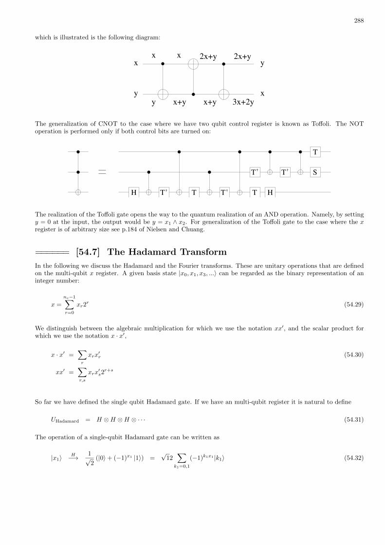
288

which is illustrated is the following diagram:

y

xx

x+y x+yy

x 2x+y 2x+y

3x+2yx

y

The generalization of CNOT to the case where we have two qubit control register is known as Toffoli. The NOToperation is performed only if both control bits are turned on:

TT T TH

T T S

T

H

The realization of the Toffoli gate opens the way to the quantum realization of an AND operation. Namely, by settingy = 0 at the input, the output would be y = x1 ∧ x2. For generalization of the Toffoli gate to the case where the xregister is of arbitrary size see p.184 of Nielsen and Chuang.

====== [54.7] The Hadamard Transform

In the following we discuss the Hadamard and the Fourier transforms. These are unitary operations that are definedon the multi-qubit x register. A given basis state |x0, x1, x3, ...〉 can be regarded as the binary representation of aninteger number:

x =

nc−1∑r=0

xr2r (54.29)

We distinguish between the algebraic multiplication for which we use the notation xx′, and the scalar product forwhich we use the notation x · x′,

x · x′ =∑r

xrx′r (54.30)

xx′ =∑r,s

xrx′s2r+s

So far we have defined the single qubit Hadamard gate. If we have an multi-qubit register it is natural to define

UHadamard = H ⊗H ⊗H ⊗ · · · (54.31)

The operation of a single-qubit Hadamard gate can be written as

|x1〉H−→ 1√

2(|0〉+ (−1)x1 |1〉) =

√12

∑k1=0,1

(−1)k1x1 |k1〉 (54.32)

289

If we have a multi-qubit register we simply have to perform (in parallel) an elementary Hadamard transform on eachqubit:

|x0, x1, ..., xr, ...〉H−→

∏r

1√2

(|0〉+ (−1)xr |1〉) =1√2nc

∏r

∑kr=0,1

(−1)krxr |kr〉

(54.33)

=1√Nc

∑k0,k1,...

(−1)k0x0+k1x1+... |k0, k1, ..., kr, ...〉 =1√Nc

∑k

(−1)k·x |k〉

The Hadmard transform is useful in order to prepare a ”democratic” superposition state as follows:

|0, 0, ..., 0〉 H−→ 1√2

(|0〉+ |1〉)⊗ 1√2

(|0〉+ |1〉)⊗ ...⊗ 1√2

(|0〉+ |1〉) 7→ 1√Nc

11...1

(54.34)

To operate with a unitary operator on this state is like making parallel computation on all the possible x basis states.

====== [54.8] The quantum Fourier transform

The definitions of the Hadamard transform and the quantum Fourier transform are very similar in style:

UHadamard|x〉 =1√Nc

∑k

(−1)k·x|k〉 (54.35)

UFourier|x〉 =1√Nc

∑k

e−i2πNckx|k〉 (54.36)

Let us write the definition of the quantum Fourier transform using different style so as to see that it is indeed aFourier transform operation in the conventional sense. First we notice that its matrix representation is

〈x′|UFourier|x〉 =1√Nc

e−i2πNcx′x (54.37)

If we operate with it on the state |ψ〉 =∑x ψx|x〉 we get |ϕ〉 =

∑x ϕx|x〉, where the column vector ϕx is obtained

from ψx by a multiplication with the matrix that represents UFourier. Changing the name of the dummy index formx to k we get the relation

ϕk =1√Nc

Nc−1∑x=0

e−i2πNckxψx (54.38)

This is indeed the conventional definition of

ψ0

ψ1

ψ2

.

.

.ψNc−1

FT−→

ϕ0

ϕ1

ϕ2

.

.

.ϕNc−1

(54.39)

290

The number of memory bits which are required to store these vectors in a classical register is of order N ∼ 2n. Thenumber of operations which is involved in the calculation of a Fourier transform seems to be of order N2. In factthere is an efficient “Fast Fourier Transform” (FFT) algorithm that reduces the number of required operations toN logN = n2n. But this is still an exponentially large number in n. In contrast to that a quantum computer canstore these vectors in n qubit register. Furthermore, the ”quantum” FT algorithm can perform the calculation withonly n2 log n log log n operations. We shall not review here how the Quantum Fourier transform is realized. Thiscan be found in the textbooks. As far as this presentation is concerned the Fourier transform can be regarded as acomplicated variation of the Hadamard transform.

====== [54.9] Note on analog or optical computation

A few words are in order here regarding quantum computation versus classical analog computation. In an analogcomputer every analog ”bit” can have a voltage within some range, so ideally each analog bit can store infinite amountof information. This is of course not the case in practice because the noise in the circuit defines some effective finiteresolution. Consequently the performance is not better compared with a digital computers. In this context the analogresolution is a determining factor in the definition of the memory size. Closely related is optical computation. Thiscan be regarded as a special type of analog computation. Optical Fourier Transform of a ”mask” can be obtainedon a ”screen” that is placed in the focal plane of a lens. The FT is done in one shot. However, also here we havethe same issue: Each pixel of the mask and each pixel of the screen is a hardware element. Therefore we still needan exponentially large hardware just to store the vectors. At best the complexity of FT with optical computer is oforder 2n.

====== [54.10] The UM operation

The CNOT/Toffoli architecture can be generalized so as to realize any operation of the type y = f(x1, x2, ...), as anx-controlled operation, where y is a single qubit. More generally we have

x = (x0, x1, x2...xnc−1) (54.40)

y = (y0, y1, y2, ...yn−1) (54.41)

and we would like to realize a unitary controlled operation

U =∑x

|x〉〈x| ⊗ U (x) ≡ P (0) ⊗ U (0) + P (1) ⊗ U (1) + P (2) ⊗ U (2) + ... (54.42)

This is formally like a measurement of the x register by the y register. Note that x is a constant of motion, and thatU has a block diagonal form:

〈x′, y′|U |x, y〉 = δx′,xU(x)y′,y =

U (0)

U (1)

U (2)

...

(54.43)

Of particular interest is the realization of a unitray operation that maps y = 1 to y = f(x). Let us look on

U(x)M

∣∣∣y⟩ =∣∣∣Mxy mod (N)

⟩(54.44)

If M is co-prime to N , then U is merely a permutation matrix, and therefore it is unitary. The way to realize thisoperation is implied by the formula

Mx = M∑s xs2

s

=∏s

(M2s

)xs=

nc−1∏s=0

Mxss (54.45)

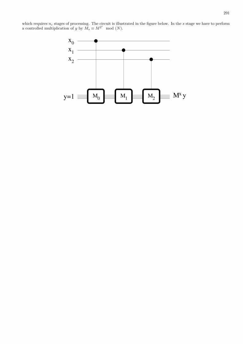
291

which requires nc stages of processing. The circuit is illustrated in the figure below. In the s stage we have to performa controlled multiplication of y by Ms ≡M2s mod (N).

x1x2

M1 M2M0

x0

xM yy=1

292

[55] The foundation of statistical mechanics

====== [55.1] The canonical formalism

Consider some system, for example particles that are confined in a box. The Hamiltonian is

H = H(r,p;X) (55.1)

where X is some control parameter, for example the length of the box. The energy of the system is defined as

E ≡ 〈H〉 = trace(Hρ) =∑r

prEr (55.2)

where is the last equality we have assume that we are dealing with a stationary state. Similarly the expression forthe generalized force y is

y ≡⟨−∂H∂X

⟩=

∑r

pr

(− ErdX

)(55.3)

It is argued that the weak interaction with an environment that has a huge density of state %env leads after relaxationto a canonical state which is determined by the parameter β = d log(%env(E))/dE that characterizes the environment.The argument is based on the assumption that the universe (system+environment) is a closed system with some totalenergy Etotal. After ergodization the system get into a stationary-like state. The probability pr to find the system instate Er is proportional to %env(Etotal−Er) ≈ %env(Etotal)e

−βEr . Accordingly

pr =1

Ze−βEr (55.4)

where the so-called partition function provides the normalization

Z (β;X) =∑r

e−βEr (55.5)

One observes that the energy can be obtained from

E = −∂ lnZ

∂β(55.6)

while the generalized force is

y =1

β

∂ lnZ

∂X(55.7)

If we slightly change X and β and assume that the state of the system remains canonical then

dE =∑r

dprEr +∑

prdEr ≡ TdS − ydX (55.8)

where the absolute temperature is defined as the integration factor of the first term

T = integration factor =1

β(55.9)

293

and the implied definition of the thermodynamic entropy is

S = −∑

pr ln pr (55.10)

Note that the thermodynamic entropy is an extensive quantity in the thermodynamic limit. At this state it isconvenient to define the Helmholtz generating function

F (T,X) ≡ − 1

βlnZ(β;X) (55.11)

which allows to write the state equation in an elegant way:

S = −∂F∂T

(55.12)

y = − ∂F∂X

(55.13)

and

E = F + TS (55.14)

====== [55.2] Work

In the definition of work the system and the environment are regarded as one driven closed unit. On the basis of the“rate of change formula” we have the following exact expression:

W = −∫〈F 〉t dX (55.15)

where F = −dH/dX. Note that 〈F〉t is calculated for the time dependent (evolving) state of the system. From linearresponse theory of driven closed systems we know that in leading order

〈F〉t ≈ 〈F〉X − ηX (55.16)

The first terms is the conservative force, which is a function of X alone. The subscript implies that the expectationvalue is taken with respect to the instantaneous adiabatic state. The second term is the leading correction to theadiabatic approximation. It is the “friction” force which is proportional to the rate of the driving. The net conservativework is zero for a closed cycle while the “friction” leads to irreversible dissipation of energy with a rate ηX2.

The above reasoning implies that for a quasi static process we can calculate the work as the sum of two contributions:W = −W +Wirreversible. The conservative work is defined as

W =

∫ B

A

y(X)dX (55.17)

The rate of irreversible work is

Wirreversible = ηX2 (55.18)

where η is the “friction” coefficient, which can be calculated using linear response theory.

294

====== [55.3] Heat

In order to understand which type of statements can be extracted form the canonical formalism we have to discusscarefully the physics of work and heat. We distinguish between the system and the environment and write theHamiltonian in the form

Htotal = H(r,p;X(t)) +Hint +Henv (55.19)

It is implicit that the interaction term is extremely small so it can be ignored in the calculation of the total energy.We define

W = work ≡(〈Htotal〉B − 〈Htotal〉A

)(55.20)

Q = heat ≡ −(〈Henv〉B − 〈Henv〉A

)(55.21)

Efinal − Einitial ≡ 〈H〉B − 〈H〉A = Q + W (55.22)

If for a general process we know the work W and the change in the energy of the system, then we can deducewhat was the heat flow Q. If we compare dE = TdS − ydX with the expression dE = dQ + dW we deduce thatTdS = dQ+dWirreversible. This implies that the change in the entropy of the system is dS = (dQ+dWirreversible)/T .

====== [55.4] The second law of thermodynamics

The discussion of irreversible processes has been differed to Lecture Notes in Statistical Mechanics and Mesoscopic,arXiv:1107.0568

====== [55.5] Fluctuations

The partition function and hence the thermodynamic equations of state give information only on the spectrum Enof the system. In the classical context this observation implies that a magnetic field has no influence on the equilibriumstate of a system because the spectrum remains E = mv2/2 with 0 < |v| <∞. In order to probe the dynamics we haveto look on the fluctuations S(t) = 〈F(t)F(0)〉, where F is some observable. The Fourier transform of S(t) describesthe power spectrum of the fluctuations:

S(ω) =

∫ ∞−∞

S(t)eiωτdτ =∑n

pn∑m

|Fmn|2 2πδ (ω − (Em−En)) (55.23)

This is the same object that appears in the Fermi-Golden-rule for the rate of transitions due to a perturbationterm V = −f(t)F . In the above formula ω > 0 corresponds to absorption of energy (upward transitions), whileω < 0 corresponds to emission (downward transitions). It is a straightforward algebra to show that for a canonicalpreparations with pn ∝ exp(−En/T ) there is a detailed balance relation:

S(ω) = S(−ω) exp

(~ωT

)(55.24)

This implies that if we couple to the system another test system (e.g. a two level “thermometer”) it would be drivenby the fluctuations into a canonical state with the same temperature.

The connection with Fermi-Golden-rule is better formalized within the framework of the so called fluctuation-dissipation relation. Assume that the system is driven by varying a parameter X, and define F as the associatedgeneralized force. The Kubo formula (see Dynamics and driven systems lectures) relates the response kernel to S(t).In particular the dissipation coefficient is:

η(ω) =S(ω)− S(−ω)

2ω(55.25)

295

If the system is in a canonical state it follow that the zero frequency response is η0 = S(0)/(2T ). If we further assume“Ohmic response”, which means having constant η(ω) = η0 up to some cutoff frequency, then the above relation canbe inverted:

Sohmic(ω) = η02ω

1− e−ω/T(55.26)

The best known application of this relation is known as the Nyquist theorem. If a ring is driven by an electro-motiveforce −Φ, then the rate of heating is W = GΦ2, which is know as Joule law. The generalized force which is associatedwith Φ is the current I, and G is known as the conductance. Note that Joule law is equivalent to Ohm law 〈I〉 = −GΦ.It follows from the fluctuation-dissipation relation that the fluctuations of the current at equilibrium for ω T aredescribed by S(ω) = 2GT . It should be clear that in non-equilibrium we might have extra fluctuations, which in thisexample are known as shot noise.

====== [55.6] The modeling of the environment

It is common to model the environment as a huge collection of harmonic oscillators, and to say that the system issubject to the fluctuations of a field variable F which is a linear combination of the bath coordinates:

F =∑α

cαQα =∑α

cα

(1

2mαωα

)1/2

(aα + a†α) (55.27)

For preparation of the bath in state n = nα we get

S(ω) =∑α

∑±c2α |〈nα±1|Qα|nα〉|2 2πδ(ω ∓ ωα) (55.28)

Using

〈nα+1|Qα|nα〉 =

(1

2mαωα

)1/2 √1 + nα (55.29)

〈nα−1|Qα|nα〉 =

(1

2mαωα

)1/2 √nα (55.30)

we get

S(ω) =∑α

1

2mαωα2πc2α

[(1+nα)δ(ω − ωα) + nαδ(ω + ωα)

](55.31)

For a canonical preparation of the bath we have 〈nα〉 = f(ωα) ≡ 1/(eω/T − 1). It follows that

S(ω) = 2J(|ω|)×

(1 + f(ω))f(−ω)

= 2J(ω)1

1− e−βω(55.32)

where we used f(−ω) = −(1 + f(ω)), and defined the spectral density of the bath as

J(ω) =π

2

∑α

c2αmαωα

δ(ω − ωα) (55.33)

with anti-symmetric continuation. For an Ohmic bath J(ω) = ηω, with some cutoff frequency ωc.