. .

LECTURE NOTESinCOMPUTATIONAL LINEAR ALGEBRAwithMATHEMATICA

.

Tadeusz STYS

MSc. & Ph.D., University of Warsaw

Email: styst@tlen.pl

Warsaw, January 2010

i

PREFACE

This text is to introduce students of science and engineering to computationallinear algebra. As a prerequisite to the numerical methods basic knowledgeof linear algebra and computing are required. Also, the text assumes a pre-vious knowledge on Mathematica as the systems for doing mathematics withcomputers. So, it is taken for granted that the reader has access to computerfacilities for solving some of examples and exercise questions.The text contains classical methods for solving linear systems of equationswith emphasis put on error analysis, algorithm design and their implementa-tion in computer arithmetic. There is also a desire that the reader will findinteresting theorems with examples solved by included Mathematica modules.The text begins with the notions and theorems concerning norms and oper-ations on vectors and matrices. In the chapter 2, direct methods for solvinglinear systems of equations based on Gauss elimination are described and sup-ported by examples and Mathematica programs.The chapter 3, contains standard methods for solving eigenvalue problemsfor quadratic matrices. It includes Jacobi method, power method, and QRmethod with examples, questions and Mathematica modules.

Iterative methods for solving linear systems of equations are presented in thechapter 4. It starts with the sufficient and necessary condition for convergenceof linear stationary one step methods. The class of linear stationary one stepmethods includes iterative Jacobi and Gauss Seidel methods, Successive Overrelaxation method (SOR), Alternating directions method (ADI) and Gradientmethod (CG).

STYS Tadeusz

ii

Contents

1 Vectors and Matrices 11.1 Vector and Matrix Norms . . . . . . . . . . . . . . . . . . . . 11.2 Conditional Number of a Matrix . . . . . . . . . . . . . . . . . 31.3 Positive Definite Matrices . . . . . . . . . . . . . . . . . . . . 51.4 Diagonally Dominant Matrices . . . . . . . . . . . . . . . . . . 61.5 Monotone Matrices . . . . . . . . . . . . . . . . . . . . . . . . 81.6 Matrices of Positive Type . . . . . . . . . . . . . . . . . . . . 91.7 Exercises . . . . . . . . . . . . . . . . . . . . . . . . . . . . . . 11

2 Systems of Linear Equations 132.1 Gauss Elimination Method . . . . . . . . . . . . . . . . . . . . 132.2 Partial Pivoting . . . . . . . . . . . . . . . . . . . . . . . . . . 202.3 Principal Element Strategy . . . . . . . . . . . . . . . . . . . . 252.4 LU-Decomposition. . . . . . . . . . . . . . . . . . . . . . . . . 282.5 Root Square Method . . . . . . . . . . . . . . . . . . . . . . . 302.6 Gauss Elimination for Tri-diagonal Matrices. . . . . . . . . . . 322.7 Gauss Elimination for Block Tri-diagonal Matrices . . . . . . . 342.8 Gauss Elimination for Pentediagonal Matrices. . . . . . . . . . 392.9 Exercises . . . . . . . . . . . . . . . . . . . . . . . . . . . . . . 42

3 Eigenvalues and Eigenvectors of a Matrix 473.1 Eigenvalue Problem . . . . . . . . . . . . . . . . . . . . . . . . 473.2 Jacobi Method for Real and Symmetric Matrices . . . . . . . . 523.3 Power Method . . . . . . . . . . . . . . . . . . . . . . . . . . . 603.4 The Householder Transformation and Hessenberg Matrices . . 643.5 QR Method . . . . . . . . . . . . . . . . . . . . . . . . . . . . 703.6 Exercises . . . . . . . . . . . . . . . . . . . . . . . . . . . . . . 79

4 Iterative Methods for Systems of Linear Equations 814.1 Stationary One Step Linear Methods . . . . . . . . . . . . . . 814.2 Jacobi Iterative Method . . . . . . . . . . . . . . . . . . . . . 834.3 Gauss Seidel Iterative Method . . . . . . . . . . . . . . . . . . 864.4 Successive Overrelaxation Method (SOR) . . . . . . . . . . . . 914.5 Alternating Direction Implicit Method (ADI) . . . . . . . . . 95

iii

iv

4.6 Conjugate Gradient Method (CG) . . . . . . . . . . . . . . . . 984.7 Exercises . . . . . . . . . . . . . . . . . . . . . . . . . . . . . . 1034.8 References . . . . . . . . . . . . . . . . . . . . . . . . . . . . . 106

Chapter 1

Vectors and Matrices

1.1 Vector and Matrix Norms

Let x = (x1, x2, ..., xn) ∈ Rn be a vector. Below, we shall consider the followingthree vector norms:

1. ‖ x ‖S=√

| x1 |2 + | x2 |2 · · ·+ | xn |2,

2. ‖ x ‖1=| x1 | + | x2 | · · ·+ | xn |,

3. ‖ x ‖∞= max1≤i≤n

| xi | .

The above vector norms satisfy the inequalities:

‖ x ‖S≤‖ x ‖1≤√n ‖ x ‖S,

‖ x ‖∞≤‖ x ‖S≤√n ‖ x ‖∞,

‖ x ‖∞≤‖ x ‖1≤ n ‖ x ‖∞,

(1.1)

Let us note that if x is an approximate vector to a vector x thenthe absolute error

ǫx =‖ x− x ‖and the relative error

δx =‖ x− x ‖‖ x ‖ , x 6= 0.

Evidently, the relative error measured in the ∞− norm expresses the numberof correct significant digits of the largest component of the approximate x. Forinstance, if

‖ x− x ‖∞‖ x ‖∞

≈ 10−6

then x should have 6 correct significant digits. If the norms ‖ − ‖S or ‖ − ‖1are used then all components of x may be biased by the error δx = 10−p.

1

2

Therefore x may have p correct significant digits.A norm of a matrix

A =

a11 a12 a13 · · · a1n−1 a1n

a21 a22 a23 · · · a2n−1 a2n

a31 a32 a33 · · · a3n−1 a3n

· · · · · · · · · · · · · · · · · ·an1 an2 an3 · · · ann−1 ann

is determined by the following relation:

‖ A ‖= supx 6=0

‖ Ax ‖‖ x ‖ .

This means that the norm ‖ A ‖ is the smallest constant for which the in-equality

‖ Ax ‖≤‖ A ‖ ‖ x ‖

holds for every x ∈ Rn.One can show that the subordinated matrix norms to the three vector normsare:

1. (a) ‖ A ‖S= max1≤i≤n

√

λi(AAT ), is the spectral norm of A, where λi(AAT )

is the i− th eigenvalue of the matrix AAT ,

(b) ‖ A ‖∞= max1≤i≤n

n∑

j=1

| aij | is the ∞− norm of A,

(c) ‖ A ‖1= max1≤j≤n

n∑

j=1

| aij | is the first norm of A,

The above matrix norms satisfy the following inequalities:

1. (a) i. 1√n‖ A ‖∞≤‖ A ‖S≤

√n ‖ A ‖∞

ii. 1√n‖ A ‖1≤‖ A ‖S≤

√n ‖ A ‖1.

Let us note that if A is a symmetric matrix then the spectral norm of A isequal to the spectral radius ρ(A), i.e.

‖ A ‖S= ρ(A),

where ρ(A) = max1≤i≤n

| λi(A) |, λi(A) is i− th eigenvalue of A.

3

1.2 Conditional Number of a Matrix

A resistance of a matrix A against perturbation of input data and round-offerrors of partial results is measured by its conditional number

Cond(A) =‖ A ‖ ‖ A−1 ‖ .

In case of a symmetric matrix A, where the spectral norm is involved, theconditional number of the matrix A is given by the formula

Cond(a) = ρ(A)ρ(A−1)

Solving numerically a system of linear equations

Ax = b,

we find an approximate solution x which is the exact solution of the system ofequations

Ax = b.

Having x, we can compute the residual absolute error

rb = Ax− Ax = b− b,

and the residual relative error

δb =||b− b||||b|| , b 6= 0.

The relative error

δx =||x− x||||x|| , x 6= 0,

satisfies the following inequality

δbCond(A)

≤ δx ≤ Cond(A) δb.

Indeed, we have

A(x− x) = b− b, x− x = A−1(b− b),

and||A|| ||x− x|| ≥ ||b− b||, ||x− x|| ≤ ||A−1|| ||b− b||.

Hence, we get

||b− b||||A|| ||x|| ≤

||x− x||x|| ≤

||A−1|| ||b− b||||x|| , x 6= 0.

4

Clearly, the solution x satisfies the inequality

||b||||A|| ≤ ||x|| ≤ ||A

−1|| ||b||.

Combining the above inequalities, we obtain

1

||A−1|| ||A||||b− b||||b|| ≤

||x− x||||x|| ≤ ||A−1|| ||A|| ||b− b||||b|| , x 6= 0, b 6= 0.

orδb

Cond(A)≤ δx ≤ Cond(A) δb.

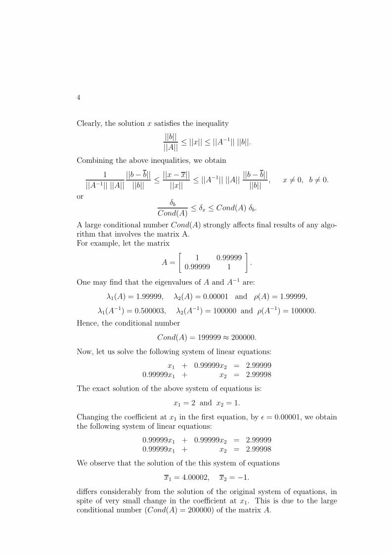
A large conditional number Cond(A) strongly affects final results of any algo-rithm that involves the matrix A.For example, let the matrix

A =

[

1 0.999990.99999 1

]

.

One may find that the eigenvalues of A and A−1 are:

λ1(A) = 1.99999, λ2(A) = 0.00001 and ρ(A) = 1.99999,

λ1(A−1) = 0.500003, λ2(A

−1) = 100000 and ρ(A−1) = 100000.

Hence, the conditional number

Cond(A) = 199999 ≈ 200000.

Now, let us solve the following system of linear equations:

x1 + 0.99999x2 = 2.999990.99999x1 + x2 = 2.99998

The exact solution of the above system of equations is:

x1 = 2 and x2 = 1.

Changing the coefficient at x1 in the first equation, by ǫ = 0.00001, we obtainthe following system of linear equations:

0.99999x1 + 0.99999x2 = 2.999990.99999x1 + x2 = 2.99998

We observe that the solution of the this system of equations

x1 = 4.00002, x2 = −1.

differs considerably from the solution of the original system of equations, inspite of very small change in the coefficient at x1. This is due to the largeconditional number (Cond(A) = 200000) of the matrix A.

5

1.3 Positive Definite Matrices

A class of positive definite matrices plays an important role in different areasof mathematics (statistics, numerical analysis, differential equations, mechan-ics, algebra, geometry, etc.). Here, we shall consider positive definite matricesfrom the numerical point of view. As it is known, the most effective numericalmethods for linear systems of equations are associated with positive definitematrices. Let us present the following definition:

Definition 1.1 A matrix A is said to be positive definite if and only if thefollowing conditions hold:

1. A is a symmetric matrix, i.e. AT = A,

2. there exists a constant γ > 0 such that

(A, x, x) =n

∑

i,j=1

aijxixj ≥ γn

∑

i=1

x2i = γ (x, x)

for every real vector x = (x1, x2, ..., xn) ∈ Rn.

Example 1.1 The matrix

A =

[

4 −1−1 4

]

is positive definite.

Evidently, A is a symmetric matrix, i.e. AT = A and

(Ax, x) = 4(x21 − x1x2 + x2

2) ≥ 2(x21 + x2

2) = 2(x, x)

for every x = (x1, x2) ∈ R2. So that γ = 2.

The following theorem holds:

Theorem 1.1 An matrix A is positive definite if and only if all its eigenvaluesare real and positive, i.e. λ1 > 0, λ2 > 0, ..., λn > 0.

Proof. At first, let us assume that A is a positive definite matrix. Then, bycondition 1, A is a symmetric matrix. Therefore all eigenvalues of A are realand eigenvectors x(1), x(2), ..., x(n) of A are orthonormal in the real space Rn.Evidently, for each eigenvector x(k), k = 1, 2, .., n; we have

0 < (Ax(k), x(k)) = λk(x(k), x(k)) = λk, k = 1, 2, ..., n.

6

Now, let us assume that all eigenvalues of A are real and positive, i.e.

0 < λ1 < λ2 <, ..., λn.

Then, each vector x 6= 0 can be presented in the form of the following linearcombination:

x = α1x(1) + α2x

(2) + . . .+ αnx(n),

where (x, x) = α21 + α2

2 + . . .+ α2n > 0.

We thus have

(Ax, x) = (An

∑

j=1

αjx(j),

n∑

j=1

αjx(j))

=n

∑

j=1

n∑

k=1

αjαk(Ax(j), x(k))

=n

∑

j=1

n∑

k=1

αjαkλj(x(j), x(k))

=n

∑

j=1

λjα2j ≥ λ1

n∑

j=1

α2j = λ1(x, x).

Hence γ = λ1. End of the proof.

1.4 Diagonally Dominant Matrices

Below, we shall show that the class of diagonally dominant matrices is a subclass of the class of positive definite matrices.

Definition 1.2 A matrix A is said to be diagonally positive dominant if andonly if the following conditions hold:

1. (a) aii ≥n

∑

j=1,j 6=i

| aij |, i = 1, 2, ..., n,

(b) there exists at least one natural i for which

aii >n

∑

j=1,j 6=i

| aij |,

(c) if condition (b) is satisfied for all i = 1, 2, .., n, then A is called astrongly diagonally dominant matrix.

Example 1.2 Evidently, the matrix

A =

4 −1 −1 0−1 4 −1 −1−1 −1 3 −1

0 −1 −1 3

7

satisfies the conditions (a) and (b) of definition and therefore, A is a diagonallypositive dominant matrix.

Let us note that conditions (a) and (b) are not difficult to check. Thus, wemay easily find whether a matrix is or is not diagonally dominant. We mayalso use these conditions to determine whether a matrix is positive definiteapplying the following theorem:

Theorem 1.2 Every non-singular symmetric and diagonally dominant matrixA is positive definite.

Proof. It is sufficient to show that all eigenvalues of matrix A are real andpositive. Then, by the theorem , A is a positive definite matrix. By assump-tion, A is a non-singular and symmetric matrix, therefore its eigenvalues arereal and different from zero.

Now, we shall show that A does not have a negative eigenvalue. Evidently,for every negative λ < 0, the matrix A− λE is strongly diagonally dominant.Therefore, the homogeneous system of linear equations

(A− λE)y = 0

has only one solution, i.e. y = 0. Indeed, let

max1≤i≤n

| yi |=| yk | .

Of course, without any additional restrictions, we may assume that yk ≥ 0.Because

0 = ak1y1 + ak2y2 + · · ·+ (akk − λ)yk + · · ·+ aknyn

≥ [(akk − λ)−n

∑

j=1,j 6=i

|akj]yk ≥ 0,

we get

[akk − λ−n

∑

j=1,j 6=i

| akj]yk = 0.

However, since A− λE, (λ < 0) is a strongly diagonally dominant matrix,

akk − λ−n

∑

j=1,j 6=i

| akj |> 0.

Hence yk = 0 and y1 = y2 = · · · = yn = 0. Thus, the matrix A − λE isnon-singular for every negative λ < 0. This means that the matrix A has allpositive eigenvalues. Finally, by the theorem , A is a positive definite matrix.

8

1.5 Monotone Matrices

Let us write the inequality A ≥ 0 if all entries of the matrix A are non-negative,i.e. aij ≥ 0, i, j = 1, 2..., n. The monotone matrices are then defined as fol-lows:

Definition 1.3 A matrix A is said to be monotone if and only if the followingimplication his true:

Ax ≥ 0 implies the inequality x ≥ 0.

The following theorem holds (cf. [18], [20]):

Theorem 1.3 A is a monotone matrix if and only if A is non-singular andthe inverse matrix to A satisfies the inequality A−1 ≥ 0.

Proof. At first, let us assume that A is a monotone matrix in the sense ofdefinition. Then, the homogeneous system of linear equations Ax = 0 has onlyone solution x = 0. Indeed, by assumption

the inequality A(±x) ≥ 0 implies the inequality ±x ≥ 0.

Hence x = 0 and therefore A is a non-singular matrix.Let z be a column of the inverse matrix A−1. Then

Az =

00...1...00

≥ 0, z ≥ 0.

Thus, the inverse matrix A−1 ≥ 0.Now, let us assume that A is a non-singular matrix and the inverse matrixA−1 ≥ 0. Then, for Ax ≥ 0, we have

x = A−1Ax ≥ 0.

Example 1.3 The matrix

A =

[

2 −1−1 2

]

is monotone.

Indeed, we have

A−1 =1

3

[

2 11 2

]

≥ 0.

9

1.6 Matrices of Positive Type

In general, it is not easy to determine, by definition, whether a matrix A ismonotone or not. However, there are so called ”matrices of positive type”which create a sub class of the class of all monotone matrices. The matrices ofpositive type are easy to investigate following the conditions of the definition:

Definition 1.4 (cf. [18]). A matrix A is said to be of positive type if andonly if the following conditions hold:

1. (a) aij ≤ 0 for i 6= j,

(b)n

∑

j=1

aij ≥ 0,

(c) there exists a non-empty subset J(A) of the set {1, 2, ..., n} suchn

∑

j=1

aij > 0 for i ∈ J(A),

(d) for every k ∈ J(A) there exists l ∈ J(A) and a sequence non-zeroentries of the form akk1

, ak1k2, ak2k3

, ..., akrl

Let us note that condition (d) can be replaced by the condition:

A is an irreducible matrix (cf. [18]).

Example 1.4 Let us consider the following matrix:

A =

2 −1 0 0 · · · 0 0−1 2 −1 0 · · · 0 0

0 −1 2 −1 · · · 0 0· · · · · · · · · · · · · · · · · · · · ·

0 0 0 0 · · · 2 −10 0 0 0 · · · −1 2

Evidently, matrix A is monotone, since it satisfies conditions (a) and (b). Also,the conditions (c) and (d) hold for the set J(A) = {1, n} while the sequenceakk1

, ak1k2, ..., akrl = −1,−1, ..− 1.

The relation between matrices that are monotone and those of positive typeis established in the following theorem (cf. [18]):

Theorem 1.4 Every matrix of positive type is a monotone matrix.

10

Proof. Let us assume that A is a matrix of positive type. Then, by conditions(a) and (b)

aii ≥ 0, i = 1, 2, ..., n.

If akk = 0 for a k ∈ {1, 2, .., n} then, (also by (a) and (b)),

akj = 0 j = 1, 2, ..., n.

However, in this case, condition (d) could not be satisfied. Therefore akk > 0for all k = 1, 2, ..., n.Now, we shall show that: the inequality Ax ≥ 0 implies the inequality x ≥ 0Indeed, by conditions (a), (b), (c) and (d)

xi ≥n

∑

j=1,j 6=i

| aij

aii

| xj , (1.2)

n∑

j=1,j 6=i

| aij

aii

|< 1 for i ∈ J(A), (1.3)

andn

∑

j=1,j 6=i

| aij

aii

= 1 for inot ∈ J(A). (1.4)

Letmin

1≤j≤nxj = xi = α < 0.

Then, by the above inequalities, we get the following contrary inequality

α = xi ≥n

∑

j=1,j 6=i

| aij

aii

| α > α for i ∈ J(A).

So that xi ≥ 0 if i ∈ J(A).If i ∈ J(A) and k 6= i then, by condition (d), aik < 0 and xk = α for all ksuch that aik < 0 or it contradicts the inequality (1.2). By condition (d), thereexists k1 such that akk1

< 0. Also, in this case when xk1= α, we have akk1

< 0or, it contradicts the inequality (1.2). Proceeding in this way, we may find asequence

akk1, ak1k2

, ak2k3, ..., akrl, l ∈ J(A),

of non-zero entries of A. But then, for l ∈ J(A), we arrive at a contradictionwith inequality (1.2). Therefore, must be α ≥ 0. Hence xk ≥ 0 for allk = 1, 2, ..., n.

Example 1.5 As we know, the following matrix is of positive type:

A =

2 −1 0 0 · · · 0 0−1 2 −1 0 · · · 0 0

0 −1 2 −1 · · · 0 0· · · · · · · · · · · · · · · · · · · · ·

0 0 0 0 · · · 2 −10 0 0 0 · · · −1 2

11

Therefore, by the theorem, A is a monotone matrix.

1.7 Exercises

Assignment Questions

Question 1. Consider the following matrix

A =

5 −2 −1 0 0 · · · 0 0

−2 5 −2 −1 0 · · · 0 0

−1 −2 5 −2 −1 · · · 0 0

· · · · · · · · · · · · · · · · · · · · · · · ·

0 0 0 0 0 · · · −2 5

Show that

(a) A is a diagonally dominant matrix

(b) A is a positive definite matrix

(c) A is of a positive type matrix

(d) A is a monotone matrix

(e) A is a Stieltjes matrix

Question 2.

(2a) Show that if A is a monotone matrix then the inverse matrix A−1 existsand A−1 ≥ 0.

(2b) Let the monotone matrices A and B satisfy the inequality A ≥ B. Showthat the inverse matrices A−1 and B−1 satisfy the inequality

B−1 ≥ A−1 ≥ 0.

(2c) Consider the following matrix

A =

4 −1 0 0 0 · · · 0 0

−1 4 −1 0 0 · · · 0 0

0 −1 4 −1 0 · · · 0 0

· · · · · · · · · · · · · · · · · · · · · · · ·

0 0 0 0 0 · · · −1 4

12

Show that A is a Stjeltjes matrix. Find the a constant γ > 0 such that(Ax, x) ≥ γ(x, x) for all real x = (x1, x2, ..., xn).

Quote the definitions and theorems used in the solution.

Chapter 2

Systems of Linear Equations

2.1 Gauss Elimination Method

Introduction. Gauss elimination is a universal direct method. In general,this method can be successfully applied to any linear system of equations, pro-vided that all arithmetic operations involved in the algorithm are not biasedby round-off errors. However, it can hardly be the case, since any imple-mentation of the method in a finite arithmetic yields round-off errors. Thus,restrictions are imposed on the class of equations because of computations ina finite arithmetic. For small systems of equations (n ≈ 100, in 8-digit floatingpoint arithmetic), Gauss method produces acceptable solutions if conditionsof stability are satisfied. The number of equations can be considerably greater(n >> 100) if partial or full pivoting strategy is applied to a stable system ofequations. For systems of equations with sparse matrices, Gauss eliminationis also successfully applicable to large systems of linear equations. Apply-ing Gauss elimination to large systems of equations, with multi-diagonal anddiagonally dominant matrices, one can obtain a solution for the number ofarithmetic operations proportional to the dimension n. This number of op-erations is significantly lower compared with the total number of arithmeticoperations ≈ n3 that is required in Gauss elimination when it is applied to asystem of equations with a full and non-singular matrix A. Although, Gaussmethod in its general form is costly in terms of arithmetic operations, themethod provides LU − decomposition of the matrix A and the determinantdet(A), as partial results in computing of the solution x.Gauss elimination. We shall write a linear system of n equations in thefollowing form:

a11x1 + a12x2 + a13x3 + · · ·+ a1nxn = a1n+1

a21x1 + a22x2 + a23x3 + · · ·+ a2nxn = a2n+1

a31x1 + a32x2 + a33x3 + · · ·+ a3nxn = a3n+1

· · · · · · · · · · · · · · · · · · · · · · · · · · · · · · · · · · · · · · · · · ·an1x1 + an2x2 + an3x3 + · · ·+ annxn = ann+1

(2.1)

13

14

or in the matrix formAx = a,

where the vectors are:

x =

x1

x2

x3...xn

, a =

a1n+1

a2n+1

a3n+1...ann+1

and the matrix is:

A =

a11 a12 a13 · · · a1n−1 a1n

a21 a22 a23 · · · a2n−1 a2n

a31 a32 a33 · · · a3n−1 a3n

· · · · · · · · · · · · · · · · · ·an1 an2 an3 · · · ann−1 ann

Within this chapter, we shall assume that the matrix A is non-singular, sothat det(A) 6= 0.Let us demonstrate Gauss elimination solving the following sample system offour equations with four unknowns

2x1 + x2 + 4x3 − 3x4 = 4 | m21 = 2 | m31 = 3 | m41 = 44x1 − 3x2 + x3 − 2x4 = −76x1 + 4x2 − 3x3 − x4 = 18x1 + 2x2 + x3 − 2x4 = 7

(2.2)

First step of elimination. At first step, we shall eliminate unknown x1 fromsecond, third and fourth equations. To eliminate x1 from second equation, wemultiply first equation by the coefficient

m21 =a21

a11=

4

2= 2

and subtract the result from second equation. Then, we have

−5x2 − 7x3 + 4x4 = −15.

To eliminate x1 from third equation, we multiply first equation by the coeffi-cient

m31 =a31

a11

=6

2= 3

and subtract the result from third equation. Then, we have

x2 − 15x3 + 8x4 = −11.

15

To eliminate x1 from fourth equation, we multiply first equation by the coef-ficient

m41 =a41

a11=

8

2= 4

and subtract the result from fourth equation. Then, we have

−2x2 − 15x3 + 10x4 = −9.

After first step of elimination, we arrive atFirst reduced system of equations

2x1 +x2 +4x3 −3x4 = 4−5x2 −7x3 +4x4 = −15 | m32 = −1

5| m42 = 2

5x2 −15x3 +8x4 = −11

−2x2 −15x3 +10x4 = −9

(2.3)

Second step of elimination. At second step, we shall eliminate x2 in (2.3) fromthird and fourth equations. To eliminate x2 from third equation, we multiplysecond equation by the coefficient

m32 =a

(1)32

a(1)22

=1

−5

and subtract the result from third equation. Then, we have

−82

5x3 +

44

5x4 = −14.

To eliminate x2 from fourth equation, we multiply second equation by thecoefficient

m42 =a

(1)42

a(1)22

=−2

−5

and subtract the result from fourth equation. Then, we have

−61

5x3 +

42

5x4 = −3.

After second step of elimination, we arrive atSecond reduced system of equations

2x1 + x2 + 4x3 − 3x4 = 4− 5x2 − 7x3 + 4x4 = −15

− 82

5x3 +

44

5x4 = −14 | m43 =

61

82

− 61

5x3 +

42

5x4 = −3

(2.4)

16

Third step of elimination. At third step, we shall eliminate x3 in (2.4) fromfourth equation. To eliminate x3 from fourth equation, we multiply thirdequation by the coefficient

m43 =a

(2)43

a(2)33

=61

82

and subtract from fourth equation.Then, we have

76

41x4 =

304

41.

Finally, we have arrived atThird reduced system of equations

2x1 + x2 + 4x3 − 3x4 = 4− 5x2 − 7x3 + 4x4 = −15

− 82

5x3 +

44

5x4 = −14

76

41x4 =

304

41

(2.5)

Let us observe that third reduced system of equations has upper-triangularform and its solution can be easily found by backward substitution. Indeed,from fourth equation

x4 =304417641

= 4,

from third equation

x3 = − 5

82(−14− 44

54) = 3,

from second equation

x2 = −1

5(−15 + 7 ∗ 3− 4 ∗ 4) = 2,

and from first equation

x1 =1

2(4− 1 ∗ 2− 4 ∗ 3 + 3 ∗ 4) = 1.

Solving this example with the Mathematica program

n=4;

a={{2,1,4,-3,4},{4,-3,1,-2,-7},{6,4,-3,-1,1},{8,2,1,-2,7}};

fi[a_,i_]:=ReplacePart[a,a[[i]]- a[[s]]*a[[i,s]]/a[[s,s]],i];

iter[a_,s_]:=Fold[fi,a,Range[s+1,n]];

Do[a=iter[a,s],{s,1,n}];

MatrixForm[a]

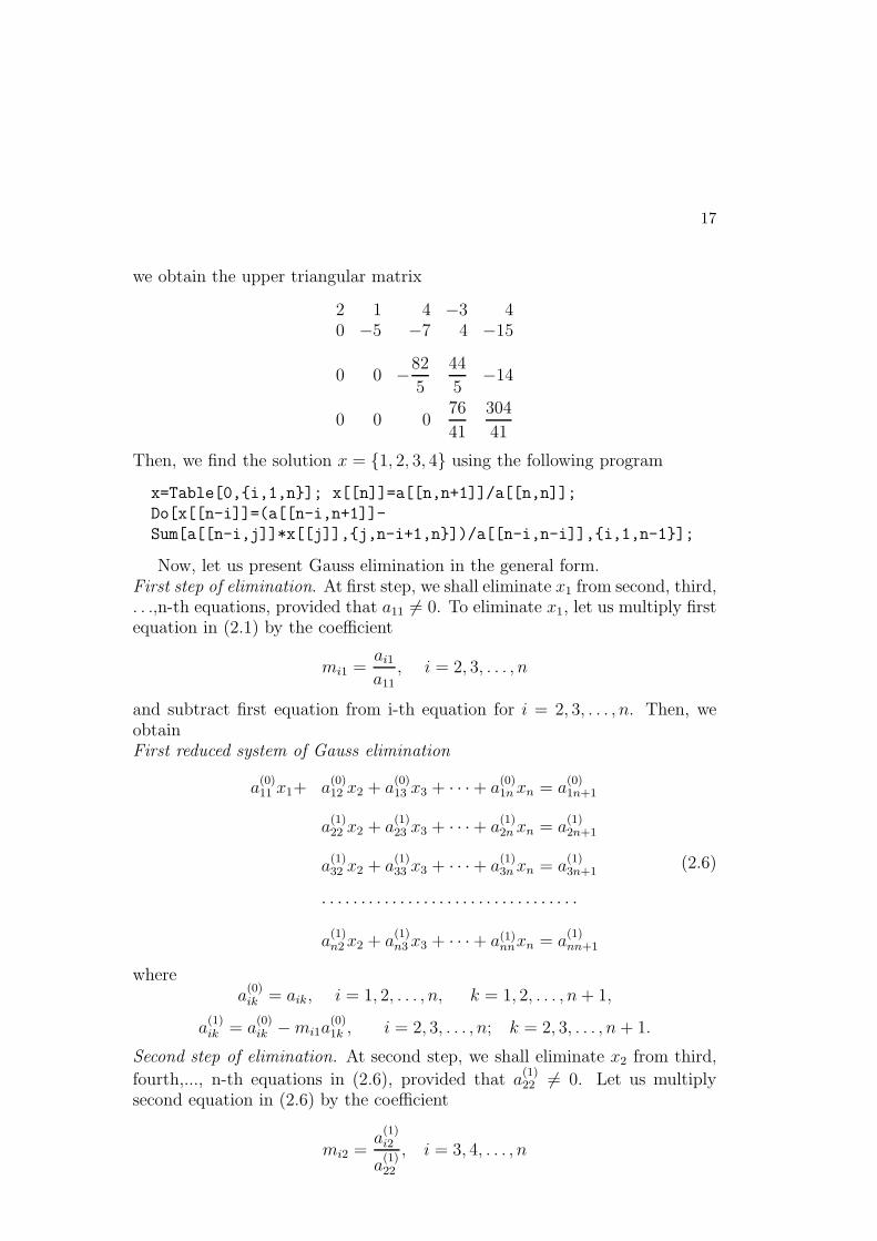
17

we obtain the upper triangular matrix

2 1 4 −3 40 −5 −7 4 −15

0 0 −82

5

44

5−14

0 0 076

41

304

41

Then, we find the solution x = {1, 2, 3, 4} using the following program

x=Table[0,{i,1,n}]; x[[n]]=a[[n,n+1]]/a[[n,n]];

Do[x[[n-i]]=(a[[n-i,n+1]]-

Sum[a[[n-i,j]]*x[[j]],{j,n-i+1,n}])/a[[n-i,n-i]],{i,1,n-1}];

Now, let us present Gauss elimination in the general form.First step of elimination. At first step, we shall eliminate x1 from second, third,. . .,n-th equations, provided that a11 6= 0. To eliminate x1, let us multiply firstequation in (2.1) by the coefficient

mi1 =ai1

a11, i = 2, 3, . . . , n

and subtract first equation from i-th equation for i = 2, 3, . . . , n. Then, weobtainFirst reduced system of Gauss elimination

a(0)11 x1+ a

(0)12 x2 + a

(0)13 x3 + · · ·+ a

(0)1n xn = a

(0)1n+1

a(1)22 x2 + a

(1)23 x3 + · · ·+ a

(1)2n xn = a

(1)2n+1

a(1)32 x2 + a

(1)33 x3 + · · ·+ a

(1)3n xn = a

(1)3n+1

· · · · · · · · · · · · · · · · · · · · · · · · · · · · · · · · ·

a(1)n2x2 + a

(1)n3 x3 + · · ·+ a(1)

nnxn = a(1)nn+1

(2.6)

wherea

(0)ik = aik, i = 1, 2, . . . , n, k = 1, 2, . . . , n+ 1,

a(1)ik = a

(0)ik −mi1a

(0)1k , i = 2, 3, . . . , n; k = 2, 3, . . . , n+ 1.

Second step of elimination. At second step, we shall eliminate x2 from third,

fourth,..., n-th equations in (2.6), provided that a(1)22 6= 0. Let us multiply

second equation in (2.6) by the coefficient

mi2 =a

(1)i2

a(1)22

, i = 3, 4, . . . , n

18

and subtract second equation from i-th equation for i = 3, 4, . . . , n. Then, weobtainSecond reduced system of Gauss elimination

a(0)11 x1+ a

(0)12 x2+ a

(0)13 x3 + · · ·+ a

(0)1nxn = a

(0)1n+1

a(1)22 x2+ a

(1)23 x3 + · · ·+ a

(1)2nxn = a

(1)2n+1

a(2)33 x3 + · · ·+ a

(2)3nxn = a

(2)3n+1

a(2)43 x3 + · · ·+ a

(2)4nxn = a

(2)4n+1

· · · · · · · · · · · · · · · · · · · · · · · · · · ·

a(2)n3x3 + · · ·+ a(2)

nnxn = a(2)nn+1

(2.7)

where

a(2)ik = a

(1)ik −mi2a

(1)2k , i = 3, 4, . . . , n, k = 3, 4, . . . , n+ 1.

We continue elimination of the unknowns x3, x4 . . . , xn−1, provided that a(2)33 6=

0, a(3)44 6= 0, a

(4)55 6= 0, ... a

(n−2)n−1n−1 6= 0. As the final step of elimination, we

obtainLast reduced system of Gauss elimination

a(0)11 x1+ a

(0)12 x2+ a

(0)13 x3+ · · · +a

(0)1n xn = a

(0)1n+1

a(1)22 x2+ a

(1)23 x3+ · · · +a

(1)2n xn = a

(1)2n+1

a(2)33 x3+ · · · +a

(2)3n xn = a

(2)3n+1

· · · · · · · · · · · · · · · · · · · · · · · ·

a(n−1)nn xn = a

(n−1)nn+1

(2.8)

where

a(s)ik = a

(s−1)ik −misa

(s−1)sk , mis =

a(s−1)is

a(s−1)ss

.

s = 1, 2 . . . , n− 1, i = s+ 1, s+ 2, . . . , n, k = s+ 1, s+ 2, . . . , n+ 1.

The system of equations (2.8) has upper-triangular form. Therefore, we caneasily find its solution by backward substitution

xn =a

(n−1)nn+1

a(n−1)nn

xi =1

a(i−1)ii

[a(i−1)in+1 −

n∑

j=i+1

a(i−1)ij xj ],

(2.9)

19

for i = n− 1, n− 2, . . . , 1.Below, we give the above elimination step by step in Mathematica.At step s, s = 1, 2, ..., n, we change i−th row of the matrix A, i = s+ 1, s+2, ..., n, by replacing it with

i−th row − s−th row ∗ i, s−th elements, s−th element

When s is fixed, the following Mathematica function would change i−th row:

oneRow[a_, i_]:=

ReplacePart[a, a[[i]]-a[[s]]*a[[i,s]]/a[[s,s]], i];

Then, the s − th iteration of Gausian elimination would require the use ofoneRow with i = s+ 1, s+ 2, ..., n, which can be achieved using Fold:

iter[a_,s_]:=Fold[oneRow, a, Range[s+1,n]];

Let us take the sample numerical example, again:

n=4;

a={{2,1,4,-3,4}, {4,-3,1,-2,-7},

{6,4,-3,-1,1},{8,2,1,-2,7}};

TableForm[a]

2 1 4 -3 4

4 -3 1 -2 -7

6 4 -3 -1 1

8 2 1 -2 7

Executing the following program

Do[oneRow[a_,i_]:=

ReplacePart[a, a[[i]]-a[[s]]*a[[i,s]]/a[[s,s]], i];

iter[a_,s_]:= Fold[oneRow, a, Range[s+1,n]];

a = iter[a, s],{s, 1, n}];

we obtain the upper triangular matrix as in (2.5).In general, the following module gaussDirectElimination solves a linear sys-tem of equations, provided that the diagonal elements a(s−1)

ss 6= 0, s = 1, 2, ..., n.

gaussDirectElimination[a_]:=Module[{c,n,oneRow,iter,x },

c=a;

n=Length[a[[1]]]-1;

oneRow[c_,i_]:=

ReplacePart[c, c[[i]]-c[[s]]*c[[i,s]]/c[[s,s]], i];

iter[c_,s_]:=Fold[oneRow, c, Range[s+1,n]];

20

Do[c= iter[c, s],{s, 1, n}];

x=Table[0,{i,1,n}]; x[[n]]=c[[n,n+1]]/c[[n,n]];

Do[x[[n-i]]=(c[[n-i,n+1]]-Sum[c[[n-i,j]]*x[[j]],

{j,n-i+1,n}])/c[[n-i,n-i]],{i,1,n-1}];

x

]

Solving the sample axample, we input data matrix

a={{2,1,4,-3,4}, {4,-3,1,-2,-7}, {6,4,-3,-1,1},{8,2,1,-2,7}};

and invoke the module

gaussDirectElimination[a]

to obtain the solution x = 1, 2, 3, 4.Let us note that, we can apply the general Gauss elimination to a system oflinear equations if the pivotal elements

a(0)11 6= 0, a

(1)22 6= 0, a

(2)33 6= 0, . . . , a(n−1n−1)

nn 6= 0,

are different from zero. Such a system of equations can be solved by theMathematica program given in the above example. However, this straightforward application of Gauss elimination might lead to a strong accumulationof round-off error. In applications, pivotal strategy is used to minimize accu-mulation of round-off errors. In the case when at least one pivotal element is

equal to zero, say a(k−1)kk = 0, we can apply partial or full pivoting strategy.

2.2 Partial Pivoting

If the pivotal element a(k−1)kk = 0 then Gauss elimination cannot be continued

without rearrangement of rows or columns of the matrix

A(k−1) =

a(0)11 a

(0)12 a

(0)13 · · · a

(0)1k · · · a

(0)1n a

(0)1n+1

a91)22 a

(1)23 · · · a

(1)2k · · · a

(1)2n a

(1)2n+1

a(2)33 · · · a

(2)3k · · · a

(2)3n a

(2)3n+1

. . .... · · · ...

...

zero element → a(k−1)kk

· · · a(k−1)kn a

(k−1)kn+1

a(k−1)k+1k

· · · a(k−1)k+1n a

(k−1)k+1n+1

......

......

largest element → a(k−1)sk

· · · a(k−1)sn a

(k−1)sn+1

......

......

a(k−1)nk

· · · a(k−1)nn a

(k−1)nn+1

21

Also, if a(k−1)kk , k = 1, 2, . . . , n− 1, are small then pivoting strategy will min-

imize affect of round-off errors on the solution. Thus, to eliminate unknownsxk, xk+1, . . . , xn, k = 1, 2, . . . , n − 1, we find the greatest absolute value ofthe elements

a(k−1)k+1k

, a(k−1)k+2k

, . . . , a(k−1)nk

,

and interchange k-th equation with s-th equation to have the pivotal element

a(k−1)sk which has the greatest absolute value on the pivotal place in k-th row

and k-th column. Then, we can continue elimination of remaining unknownsxk, xk+1, . . . , xn taking pivotal entries with the greatest absolute values. Thepartial pivoting strategy always succeeds, if A is a non-singular matrix. Partialpivoting can be also done with interchange of relevant columns in matrix A.Then, the greatest absolute values of elements

a(k−1)kk , a

(k−1)kk+1 , . . . , a

(k−1)kn

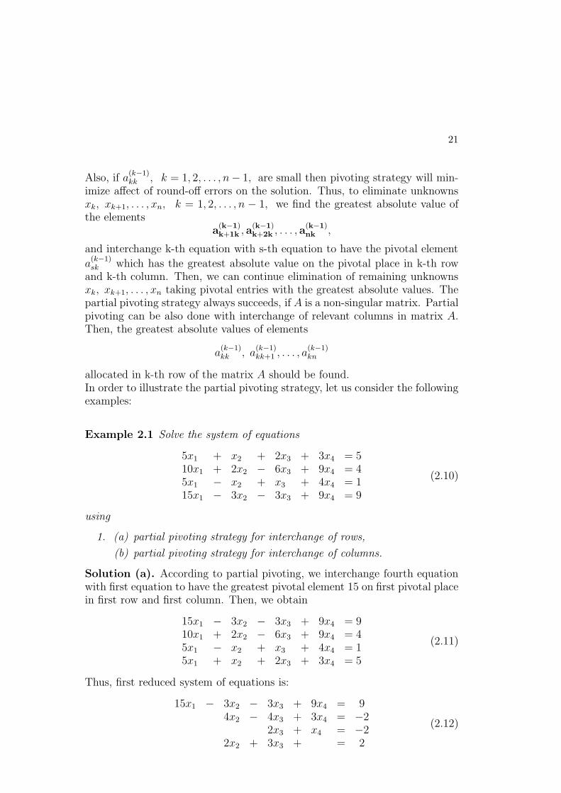
allocated in k-th row of the matrix A should be found.In order to illustrate the partial pivoting strategy, let us consider the followingexamples:

Example 2.1 Solve the system of equations

5x1 + x2 + 2x3 + 3x4 = 510x1 + 2x2 − 6x3 + 9x4 = 45x1 − x2 + x3 + 4x4 = 115x1 − 3x2 − 3x3 + 9x4 = 9

(2.10)

using

1. (a) partial pivoting strategy for interchange of rows,

(b) partial pivoting strategy for interchange of columns.

Solution (a). According to partial pivoting, we interchange fourth equationwith first equation to have the greatest pivotal element 15 on first pivotal placein first row and first column. Then, we obtain

15x1 − 3x2 − 3x3 + 9x4 = 910x1 + 2x2 − 6x3 + 9x4 = 45x1 − x2 + x3 + 4x4 = 15x1 + x2 + 2x3 + 3x4 = 5

(2.11)

Thus, first reduced system of equations is:

15x1 − 3x2 − 3x3 + 9x4 = 94x2 − 4x3 + 3x4 = −2

2x3 + x4 = −22x2 + 3x3 + = 2

(2.12)

22

To get second reduced system, we do not need to make any interchange since

a(1)22 = 4 is the greatest entry in 2-nd column on the pivotal place. Thus, second

reduced system is:

15x1 − 3x2 − 3x3 + 9x4 = 94x2 − 4x3 + 3x4 = −2

2x3 + x4 = −25x3 − 3

2x4 = 3

(2.13)

Obviously, third (last) reduced system of equations has upper-triangular form

15x1 − 3x2 − 3x3 + 9x4 = 94x2 − 4x3 + 3x4 = −2

5x3 − 1.5x4 = 3− 1.6x4 = 3.2

(2.14)

Hence, the solution is

x4 = −2,

x3 =1

2[−2− (−2)] = 0,

x2 =1

4[−2 + 4 ∗ 0− 3 ∗ (−2)] = 1,

x1 =1

15[9 + 3 ∗ 1 + 3 ∗ 0− 9 ∗ (−2)] = 2.

Solution (b). Let us come back to the original system of equations (2.10).

Evidently, the entry a(0)11 = 5 has greatest absolute value among all entries in

first row of A. Therefore, there is no a need to interchange columns in A.Then, we obtainFirst reduced system of equations:

5x1 + 2x2 + x3 + 3x4 = 5− 10x3 + 3x4 = −6

− 2x2 − x3 + x4 = −4− 6x2 − 9x3 + = −6

(2.15)

We shall interchange second and fourth equations in (2.15) to obtain the fol-lowing system of equations:

5x1 + x2 + 2x3 + 3x4 = 5− 6x2 − 9x3 = −6− 2x2 − x3 + x4 = −4

− 10x3 + 3x4 = −6

(2.16)

23

Next, we shall interchange second and third columns in (2.16) to get the pivotal

entry a(1)22 = −9 on the pivotal place in second row and second column.

5x1 + 2x3 + x2 + 3x4 = 5− 9x3 − 6x2 = −6− x3 − 2x2 + x4 = −4− 10x3 + 3x4 = −6

(2.17)

Now, we shall eliminate x3 from third and fourth equations in (2.17) to obtainthe second reduced system of equations:

5x1 + 2x3 + x2 + 3x4 = 5− 9x3 − 6x2 = −6

− 4

3x2 + x4 = −10

320

3x2 + 3x4 =

2

3

(2.18)

The pivotal entry a(2)33 = −4

3has the greatest absolute value in first row of the

matrix

A(2) =

−4

31

20

33

.

Therefore, according to the partial pivoting, we shall not make any change ofcolumns to eliminate x2 from fourth equation in (2.18). Then, we obtain third(last) reduced system of equations:

5x1 + 2x3 + x2 + 3x4 = 5− 9x3 − 6x2 = −6

− 4

3x2 + x4 = −10

3

8x4 = −16

(2.19)

Hence, by backward substitution, we find the solution

x4 = −2,

x2 = −3

4[−10

3− 2 ∗ (−2)] = 1,

x3 = −1

9[−6 + 6 ∗ 1] = 0,

x1 =1

5[5− 2 ∗ 0− 1− 3(−2)] = 2.

In the programming approach to the partial pivoting on rows, in Mathematica,we shall use the following algorithm

24

1. Set the matrix m = [a|b] that includes right side vector b and the emptylist {}.

2. Find the maximum element in the first column of m and denote it bymk.

3. Denote by k the position of mk in the first column of m.

4. Set rowk = m[[k]]/mk

5. Append rowk to e.

6. Drop k-th row of m.

7. Replace each row of m by the row − rowk ∗ First[row]

8. Drop first column of m

9. Return {m, e}.

10. Nest stepstt 1 - 7 n times, where n is the number of rows in m.

The Mathematica module eliminatepivo based on the partial pivoting re-duces a system of algebraic equations to the upper triangular form and givesits solution.

eliminatepivo[a_, b_]:= Module[

{oneIter, mat, elimMatrix},

oneIter[{m_,e_}]:= Module[

{column1, mk, k, rowk, changeOneRow},

column1=Map[First[#]&, m];

mk= Max[column1];

{{k}}= Position[column1, mk];

rowk= m[[k]]/mk;

changeOneRow[row_]:= row - rowk*First[row];

{Map[Rest[#]&,

Map[changeOneRow, Drop[m, {k}]]] ,

Append[e, Rest[rowk]]} ];

mat = Transpose[ Append[Transpose[a], b]];

{{}, elimMatrix}=

Nest[oneIter, {mat, {}}, Length[First[mat]]-1];

25

Fold[Prepend[#1, Last[#2] - Drop[#2, -1] . #1]&,

Last[elimMatrix],

Rest[Reverse[elimMatrix]]]

]

To solve the system of equations (2.11) using the module eliminatepivo, weinput data

m={{5,1,2,3,},{10,2,-6,9},{5,-1,1,4},{15,-3,-3,9}};

b={5,4,1,9}

and invoke the module eliminatepivo[m,b].

2.3 Principal Element Strategy

We apply principal element strategy to operate with possibly greatest pivotalentries in Gauss elimination. First, we find the greatest absolute value ofentries in matrix A. Let

|ars| = max1≤i,j≤n

|aij |.

Then, we interchange first row with r-th row and first column with s-th col-umn to place the greatest value as first pivotal element. We should renumer-ate equations and unknowns, respectively. Next, we eliminate the relevantunknown from second, third,. . .,n-th of the newly renumerate equations to getfirst reduced system of equations. Secondly, we find the greatest absolute value

among the entries a(1)ij , i, j = 2, 3, . . . , n. Let

| a(1)rs |= max

2≤i,j≤n| a(1)

ij | .

Then, we interchange second row with the r-th row and second column with s-th column to place the greatest pivotal entry on second row and second column.We should renumerate equations and unknowns, again. After, elimination ofx2 from third, fourth,. . . , n − th equations, we get second reduced system ofequations. We repeat this process till upper-triangular systems appears.

Example 2.2 Solve the system of equations

5x1 + x2 + 2x3 + 3x4 = 510x1 + 2x2 − 6x3 + 9x4 = 45x1 − x2 + x3 + 4x4 = 115x1 − 2x2 − x3 + 10x4 = 8

(2.20)

using full pivoting strategy.

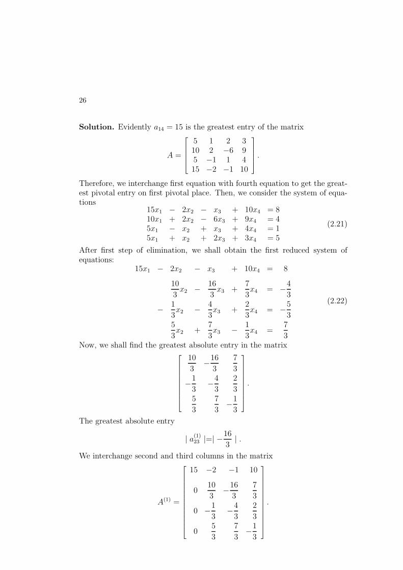
26

Solution. Evidently a14 = 15 is the greatest entry of the matrix

A =

5 1 2 310 2 −6 95 −1 1 415 −2 −1 10

.

Therefore, we interchange first equation with fourth equation to get the great-est pivotal entry on first pivotal place. Then, we consider the system of equa-tions

15x1 − 2x2 − x3 + 10x4 = 810x1 + 2x2 − 6x3 + 9x4 = 45x1 − x2 + x3 + 4x4 = 15x1 + x2 + 2x3 + 3x4 = 5

(2.21)

After first step of elimination, we shall obtain the first reduced system ofequations:

15x1 − 2x2 − x3 + 10x4 = 8

10

3x2 −

16

3x3 +

7

3x4 = −4

3

− 1

3x2 − 4

3x3 +

2

3x4 = −5

35

3x2 +

7

3x3 − 1

3x4 =

7

3

(2.22)

Now, we shall find the greatest absolute entry in the matrix

10

3−16

3

7

3

−1

3−4

3

2

35

3

7

3−1

3

.

The greatest absolute entry

| a(1)23 |=| −

16

3| .

We interchange second and third columns in the matrix

A(1) =

15 −2 −1 10

010

3−16

3

7

3

0 −1

3−4

3

2

3

05

3

7

3−1

3

.

27

to get the greatest absolute pivotal entry on the pivotal place in second row andin second column. Then, x2 takes the position of x3 and x3 takes the positionof x2. For second step of elimination, we consider the following system ofequations:

15x1 − x3 − 2x2 + 10x4 = 8

− 16

3x3 +

10

3x2 +

7

3x4 = −4

3

− 4

3x3 − 1

3x2 +

2

3x4 = −5

37

3x3 +

5

3x2 − 1

3x4 =

7

3

(2.23)

Now, we shall eliminate x3 from third and fourth equations in (2.23) to getsecond reduced system of equations:

15x1 − x3 − 2x2 + 10x4 = 8

− 16

3x3 +

10

3x2 +

7

3x4 = −4

3

− 7

6x2 +

1

12x4 = −4

3

+25

8x2 +

11

16x4 =

7

4

(2.24)

We us observe that a(2)43 = 25

8is the greatest entry in the matrix

−7

6

1

1225

8

11

16

Thus, we shall interchange third and fourth equations in (2.24) to get thegreatest pivotal entry on the pivotal place in third row and third column.Then, we consider the following system of equations:

15x1 − x3 − 2x2 + 10x4 = 8

− 16

3x3 +

10

3x2 +

7

3x4 = −4

3

+25

8x2 +

11

16x4 =

7

4

− 7

6x2 +

1

12x4 = −4

3

(2.25)

28

Finally, we shall eliminate x2 from fourth equation in (2.25) to get the lastreduced system of equations in the upper-triangular form

15x1 − x3 − 2x2 + 10x4 = 8

− 16

3x3 +

10

3x2 +

7

3x4 = −4

325

8x2 +

11

16x4 =

7

417

50x4 = −17

25

(2.26)

Hence, the solution is:

x4 = −2

x2 = −6

7[−4

3− 1

12(−2)] = 1

x3 = − 3

16[−4

3− 10

3− 7

3(−2)] = 0

x1 =1

15[8 + 2− 10(−2)] = 2.

2.4 LU-Decomposition.

Applying Gauss elimination method, we obtain the solution x = (x1, x2, . . . , xn)of the system of equations

Ax = a (2.27)

and the following factorized form of the matrix A:

A = LU,

where the lower triangular matrix

L =

1 0 0 0 · · · 0 0m21 1 0 0 · · · 0 0m31 m32 1 0 · · · 0 0m41 m42 m43 1 · · · 0 0· · · · · · · · · · · · · · · · · · · · ·mn1 mn2 mn3 mn4 · · · mnn−1 1

,

29

and the upper-triangular matrix

U =

a(0)11 a

(0)12 a

(0)13 a

(0)14 · · · a

(01n−1 a

(0)1n

0 a(1)22 a

(1)23 a

(1)24 · · · a

(1)2n−1 a

(1)2n

0 0 a(2)33 a

(2)34 · · · a

(2)3n−1 a

(2)3n

0 0 0 a(3)44 · · · a

(3)4n−1 a

(3)4n

· · · · · · · · · · · · · · · · · · · · ·0 0 0 0 · · · 0 a(n−1)

nn

,

Indeed, the product of i-th row of the matrix L by k-th column of the matrixU is:

n∑

s=1

LisUsk =p

∑

s=1

misa(s−1)sk ,

where p = min{i, k}.Let us note that

a(s)ik = a

(s−1)ik −misa

(s−1)sk ,

By taking the sum of both hand sides, we obtain

a(p)ik = aik −

p−1∑

s=1

misa(s−1)sk .

Hence

aik = a(p)ik +

p∑

s=1

misa(s−1)sk .

One can check that the following equalities hold:

a(p)ik = a

(i)ik if i ≤ k

anda

(p)ik = 0 if i > k.

Thus, for mii = 1, we have

aik =p

∑

s=1

misa(s−1)sk =

n∑

s=1

LisUsk.

As an example of LU decomposition, we note that the matrix of the systemof equations in (2.2) has the following LU decomposition:

A =

2 1 4 −34 −3 1 −26 4 −3 −18 2 1 −2

=

1 0 0 02 1 0 0

3 −1

51 0

42

5

61

821

2 1 4 −30 −5 −7 4

0 0 −82

5

44

5

0 0 076

41

. = LU

30

2.5 Root Square Method

It is possible to present a symmetric matrix A = {Aij}, i, j = 1, 2, ..., n as thesquare of a triangular matrix (cf. [6])

L =

L11 L12 L13 · · · L1n

0 L22 L23 · · · L2n

0 0 L33 · · · L3n

· · · · · · · · · · · · · · ·0 0 0 · · · Lnn

so that A = LTL. Indeed, we note that

Aij = L1iL1j + L2iL2j + · · ·+ LiiLij , i = 1, 2, ..., j − 1

andAii = L2

1i + L22i + · · ·+ L2

ni, i = j.

Hence

L11 =√A11, L1j =

A1j

L11, j = 2, 3, ..., n,

Lii =

√

√

√

√Aii −i−1∑

k=1

L2ki, i = 2, 3, ..., n,

Lij =1

Lii

[Aij −i−1∑

k=1

LkiLkj], j = i+ 1, i+ 2, ..., n,

Lij = 0, j = 1, 2, ..., i− 1.

The LL-decomposition algorithm always succeeds if A is a positive definitematrix. However, the algorithm is also applicable when A is a symmetric ma-trix, provided that Lii 6= 0, i = 1, 2, ..., n. In the case when complex numbersappear (Aii−

∑

L2ki < 0) the algorithm produces complex entries of the trian-

gular matrix L.Having LL-decomposition of the matrix A, we can find solution x of the systemof linear equations

Ax = b

by the substitutionLT z = b and Lx = z.

So that

z1 =b1L11

, zi =1

Lii

[bi −i−1∑

k=1

Lkizk], i = 2, 3, ..., n,

and by backward substitution

xn =zn

Lnn

, xi =1

Lii

[zi −n

∑

k=i+1

Likxk], i = n− 1, n− 2, ..., 1.

31

Example 2.3 Let us solve the following system of linear equations (cf. [6])

x1 + 0.42x2 + 0.54x3 + 0.66x4 = 0.30.42x1 + 1x2 + 0.32x3 + 0.44x4 = 0.50.54x1 + 0.32x2 + 1x3 + 0.22x4 = 0.70.66x1 + 0.44x2 + 0.22x3 + 1x4 = 0.9

using the following Mathematica module choleva

choleva[a_,b_]:=Module[{l,i,j,k,m,m1,n,x,z},

n=Length[a[[1]]];

l[1,1]:=l[1,1]=Sqrt[a[[1,1]]];

l[1, j_]:=l[1,j]=a[[1,j]]/l[1,1];

l[i_,i_]:=l[i,i]=Sqrt[a[[i,i]]- Sum[l[k,i]^2, {k, 1,i-1}]];

l[i_, j_]:=l[i,j]=

(a[[i,j]]-Sum[l[k,i] l[k,j], {k,1,i-1}])/l[i,i];

m=Table[Join[Table[0,{i-1}],Table[l[i,j],{j,i,n}]],

{i,1,n}];l[n,n];

m1=Transpose[m];

z[1]=b[[1]]/m1[[1,1]];

z[i_]:=z[i]=(b[[i]]-Sum[m1[[i,j]]*z[j],{j,1,i-1}])/m1[[i,i]];

x[n]=z[n]/m[[n,n]];

x[i_]:=x[i]=(z[i]-Sum[m[[i,j]]*x[j],{j,i+1,n}])/m[[i,i]];

Print["x = ",Table[x[i],{i,1,n}]];

Print["Matrix L =",MatrixForm[m]]

]

We input the matrix a and the right side vector b

a={{1.,0.42,0.54,0.66},{0.42,1.,0.32,0.44},

{0.54,0.32,1.,0.22},{0.66,0.44,0.22,1.}};

b={0.3,0.5,0.7,0.9};

Then, we invoke the module

choleva[a,b]

to obtain the solution

x = {-1.25779, 0.0434873, 1.03917, 1.48239}

and the upper triangular matrix

L =

1. 0.42 0.54 0.660 0.907524 0.102697 0.1793890 0 0.835376 −0.1853330 0 0 0.7056

.

32

2.6 Gauss Elimination for Tri-diagonal Matrices.

Let us note that for a tri-diagonal matrix A, the system of linear equations(2.1) takes the following form:

a11x1 + a12x2 = a1n+1

a21x1 + a22x2 + a23x3 = a2n+1

a32x2 + a33x3 + a34x4 = a3n+1

· · · · · · · · · · · · · · · · · · · · · · · · · · · · · ·aii−1xi−1 + aiixi + aii+1xi+1 = ain+1

· · · · · · · · · · · · · · · · · · · · · · · ·ann−1xn−1 + annxn = ann+1

Applying Gauss elimination to the above tri-diagonal system of equations, weobtain the last reduced system of equations:

a11x1 + a12x2 = a1n+1

a(1)22 x2 + a23x3 = a

(1)2n+1

a(2)33 x3 + a34x4 = a

(2)3n+1

· · · · · · · · · · · · · · · · · · · · · · · ·a

(i−1)ii xi + aii+1xi+1 = a

(i−1)in+1

· · · · · · · · · · · · · · ·a(n−1)

nn xn = a(n−1)nn+1

(2.28)

where (see (2.8) and (2.9))

a(i−1)ii = aii −

aii−1

a(i−2)i−1i−1

ai−1i,

a(i−1)in+1 = ain+1 −

a(i−2)i−1n+1

a(i−2)i−1i−1

aii−1,

for i = 2, 3, . . . , n.From formulae (2.9), we have

xn =a

(n−1)nn+1

a(n−1)nn

,

and

xi =1

a(i−1)ii

[a(i−1)in+1 − aii+1xi+1],

for i = n− 1, n− 2, . . . , 1.Let us denote by

αi =aii+1

a(i−1)ii

, i = 1, 2, ..., n− 1 βi =a

(i−1)in+1

a(i−1)ii

i = 1, 2, ..., n.

33

Then, we have

α1 =a12

a11

, β1 =a1n+1

a11

and

αi =aii+1

aii − αi−1aii−1, βi =

ain+1 − βi−1aii−1

aii − αi−1aii−1.

We obtain the following algorithm for solving a system of equations with atri-diagonal matrix.Algorithm.

Set :

α1 =a12

a11, β1 =

a1n+1

a11

for i = 2, 3, . . . , n− 1, evaluate :

αi =aii+1

aii − αi−1aii−1

for i = 2, 3, . . . , n, evaluate :

βi =ain+1 − βi−1aii−1

aii − αi−1aii−1

set : xn = βn

evaluate : for i = n− 1, n− 2, . . . , 1

xi = βi − αixi+1.

(2.29)

The above algorithm is stable with respect to round-off errors if the tri-diagonalmatrix A satisfies the following conditions:

a11 >| a12 |, ann >| ann−1 |,

aii ≥| aii−1 | + | aii+1 |, i = 2, 3, . . . , n− 1.

Then all α′s coefficients are less than one.Indeed, we have

| α1 |< 1

| αi |≤ |aii+1

aii − αi−1aii−1

|≤ | aii+1 || aii+1 | +(1− | αi−1 |) | aii−1 |

< 1.

for i = 2, 3, . . . , n− 1.

The solution x can be obtained by this algorithm with total number of 8n− 6arithmetic operations.

34

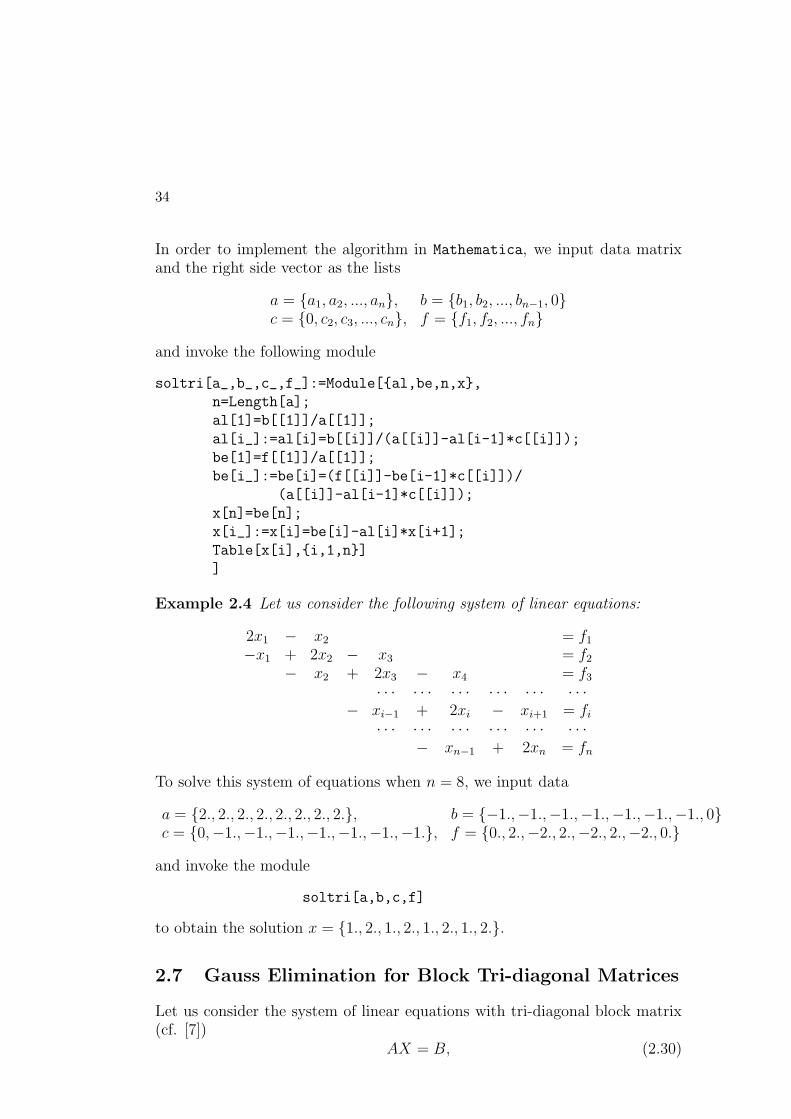
In order to implement the algorithm in Mathematica, we input data matrixand the right side vector as the lists

a = {a1, a2, ..., an}, b = {b1, b2, ..., bn−1, 0}c = {0, c2, c3, ..., cn}, f = {f1, f2, ..., fn}

and invoke the following module

soltri[a_,b_,c_,f_]:=Module[{al,be,n,x},

n=Length[a];

al[1]=b[[1]]/a[[1]];

al[i_]:=al[i]=b[[i]]/(a[[i]]-al[i-1]*c[[i]]);

be[1]=f[[1]]/a[[1]];

be[i_]:=be[i]=(f[[i]]-be[i-1]*c[[i]])/

(a[[i]]-al[i-1]*c[[i]]);

x[n]=be[n];

x[i_]:=x[i]=be[i]-al[i]*x[i+1];

Table[x[i],{i,1,n}]

]

Example 2.4 Let us consider the following system of linear equations:

2x1 − x2 = f1

−x1 + 2x2 − x3 = f2

− x2 + 2x3 − x4 = f3

· · · · · · · · · · · · · · · · · ·− xi−1 + 2xi − xi+1 = fi

· · · · · · · · · · · · · · · · · ·− xn−1 + 2xn = fn

To solve this system of equations when n = 8, we input data

a = {2., 2., 2., 2., 2., 2., 2., 2.}, b = {−1.,−1.,−1.,−1.,−1.,−1.,−1., 0}c = {0,−1.,−1.,−1.,−1.,−1.,−1.,−1.}, f = {0., 2.,−2., 2.,−2., 2.,−2., 0.}

and invoke the module

soltri[a,b,c,f]

to obtain the solution x = {1., 2., 1., 2., 1., 2., 1., 2.}.

2.7 Gauss Elimination for Block Tri-diagonal Matrices

Let us consider the system of linear equations with tri-diagonal block matrix(cf. [7])

AX = B, (2.30)

35

where the right side vector and unknown vector are:

B =

B1

B2

B3...Bn

, Bi =

Bi1

Bi2

Bi3...Bin

, X =

X1

X2

X3...Xn

, Xi =

xi1

xi2

xi3...xim

,

and the block matrix

A =

A11 A12 0 0 · · · 0 0A21 A22 A23 0 · · · 0 00 A32 A33 A34 · · · 0 0· · · · · · · · · · · · · · · · · · · · ·0 0 0 0 0 Ann−1 Ann

,

Aij =

a11ij a12

ij · · · a1mij

a21ij a22

ij · · · a2mij

· · · · · · · · · · · ·am1

ij am2ij · · · amm

ij

, i, j = 1, 2, ..., n.

Clearly, the system of equations (2.30) takes the following form in the blocknotation:

A11X1 +A12X2 = B1

A21X1 +A22X2 +A23X3 = B2

A32X2 +A33X3 +A34X4 = B3

· · · · · · · · · · · · · · · · · · · · · · · · · · · · · ·An−1n−1Xn−1 +An−1nXn = Bn−1

Ann−1Xn−1 +AnnXn = Bn

(2.31)Applying non-pivoting strategy, we can find the solution X, provided that thepivotal matrices are non-zero entries.In order to get the first reduced system of equations, we multiply from the leftfirst row-block in (2.31) by the matrix

M21 = A21A−111

providing that the inverse matrix A−111 exists. Then, we obtain

the first reduced system of equations:

A11X1 +A12X2 = B1

A(1)22 X2 +A23X3 = B

(1)2

A32X2 +A33X3 +A34X4 = B3

· · · · · · · · · · · · · · · · · · · · ·An−1n−1Xn−1 +An−1nXn = Bn−1

Ann−1Xn−1 +AnnXn = Bn

(2.32)

36

whereA

(1)22 = A22 − A21A

−111 A12,

B(1)2 = B2 − A21A

−111 B1.

Next, multiplying from the left second row-block in (2.32) by the matrix

M32 = A32A−(1)22

we obtainthe second reduced system of equations:

A11X1 +A12X2 = B1

A(1)22 X2 +A23X3 = B

(1)2

A(2)33 X3 +A34X4 = B

(2)3

· · · · · · · · · · · · · · · · · · · · ·An−1n−1Xn−1 +An−1nXn = Bn−1

Ann−1Xn−1 +AnnXn = Bn

(2.33)where

A(2)33 = A33 − A32A

−(1)22 A23,

B(2)3 = B3 − A32A

−(1)22 B

(1)2 .

We continue the block elimination process if the pivotal matrices A(i−1)ii , i =

1, 2, ..., n; are non-singular. As the final step of elimination, we obtainthe last reduced system of equations:

A11X1 +A12X2 = B1

A(1)22 X2 +A23X3 = B

(1)2

A(2)33 X3 +A34X4 = B

(2)3

· · · · · · · · · · · · · · · · · · · · ·A

(n−2)n−1n−1Xn−1 +An−1nXn = B

(n−2)n−1

A(n−1)nn Xn = B(n−1)

n

(2.34)where

A(i−1)ii = Aii −Aii−1A

−(i−2)i−1i−1Ai−1i,

B(i−1)i = Bi − Aii−1A

−(i−2)i−1i−1B

−(i−2)i−1 ,

i = 2, 3, ..., n.Hence, the solution is

Xn = A−(n−1)nn B(n−1)

n ,

Xi = A−(i−1)ii [B

(i−1)i −Aii+1Xi+1], i=n-1,n-2,...,1.

(2.35)

The following theorem holds:

37

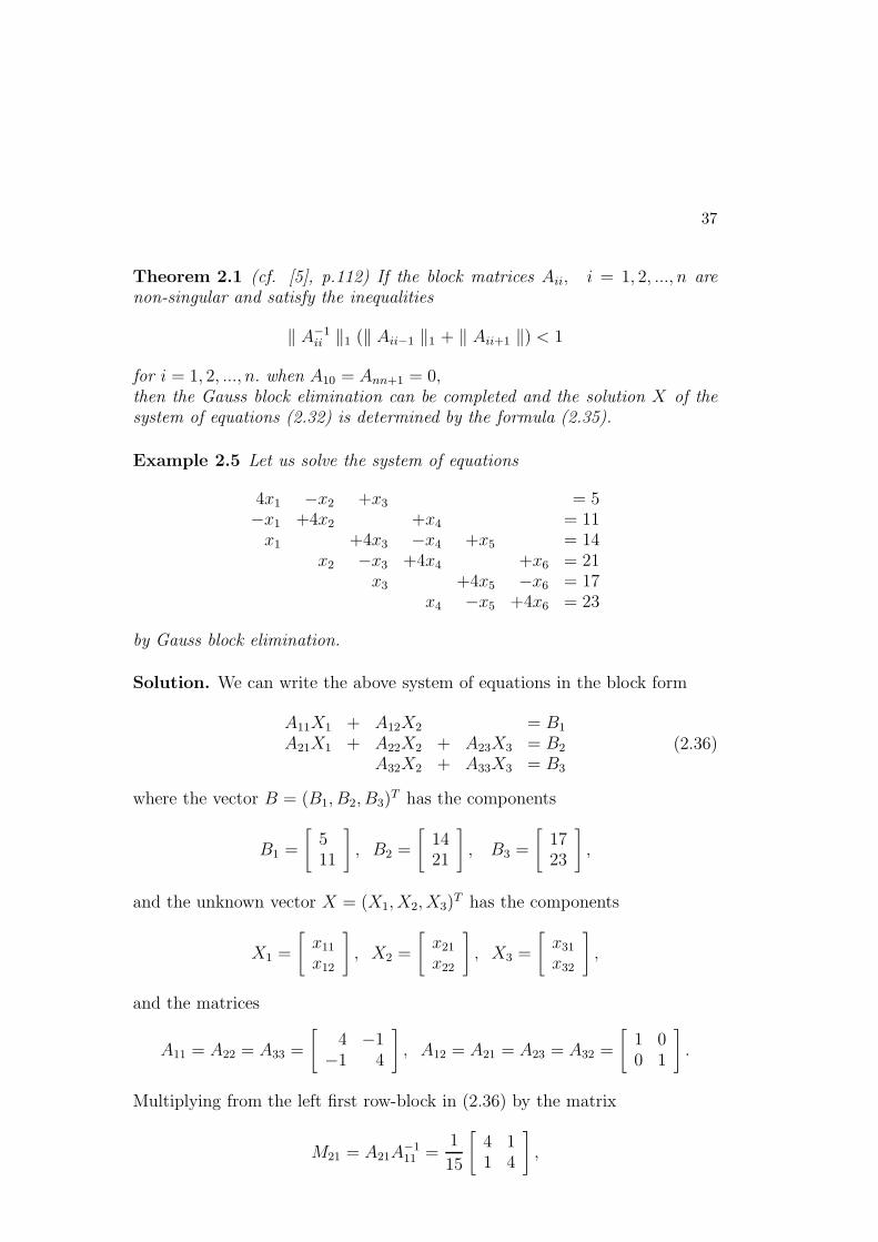
Theorem 2.1 (cf. [5], p.112) If the block matrices Aii, i = 1, 2, ..., n arenon-singular and satisfy the inequalities

‖ A−1ii ‖1 (‖ Aii−1 ‖1 + ‖ Aii+1 ‖) < 1

for i = 1, 2, ..., n. when A10 = Ann+1 = 0,then the Gauss block elimination can be completed and the solution X of thesystem of equations (2.32) is determined by the formula (2.35).

Example 2.5 Let us solve the system of equations

4x1 −x2 +x3 = 5−x1 +4x2 +x4 = 11x1 +4x3 −x4 +x5 = 14

x2 −x3 +4x4 +x6 = 21x3 +4x5 −x6 = 17

x4 −x5 +4x6 = 23

by Gauss block elimination.

Solution. We can write the above system of equations in the block form

A11X1 + A12X2 = B1

A21X1 + A22X2 + A23X3 = B2

A32X2 + A33X3 = B3

(2.36)

where the vector B = (B1, B2, B3)T has the components

B1 =

[

511

]

, B2 =

[

1421

]

, B3 =

[

1723

]

,

and the unknown vector X = (X1, X2, X3)T has the components

X1 =

[

x11

x12

]

, X2 =

[

x21

x22

]

, X3 =

[

x31

x32

]

,

and the matrices

A11 = A22 = A33 =

[

4 −1−1 4

]

, A12 = A21 = A23 = A32 =

[

1 00 1

]

.

Multiplying from the left first row-block in (2.36) by the matrix

M21 = A21A−111 =

1

15

[

4 11 4

]

,

38

and then subtracting the result from the second row-block, we obtainthe first reduced system of equations:

A11X1 + A12X2 = B1

A(1)22 X2 + A23X3 = B

(1)2

A32X2 + A33X3 = B3

(2.37)

where

A(1)22 = A22 −A21A

−111 A12 =

[

4 −1−1 4

]

− 1

15

[

4 11 4

]

=1

15

[

56 −16−16 56

]

,

B(1)2 = B2 −A21A

−111 B1 =

[

1421

]

− 1

15

[

4 11 4

] [

511

]

=1

15

[

179266

]

.

To eliminate the unknownX2 from third equation in (2.37), we multiply secondrow-block by the matrix

M32 = A32A−(1)22 =

1

24

[

7 22 7

]

and we subtract the result from third row-block in (2.37). Then, we obtainthe second reduced system of equations:

A11X1 + A12X2 = B1

A(1)22 X2 + A23X3 = B

(1)2

+ A(2)33 X3 = B

(2)3

(2.38)

where

A(2)33 = A33−A32A

−(1)22 A23 =

[

4 −1−1 4

]

− 1

24

[

7 22 7

]

=1

24

[

89 −26−26 89

]

,

B(2)3 = B3 − A−(1)

22 B(1)2 =

[

1723

]

− 1

24

[

7 22 7

]

1

15

[

179266

]

=1

24

[

289404

]

.

Hence, by formula (2.35), we obtain

X3 = A−(2)33 B

(2)3 =

24

7245

[

89 2626 89

]

1

24

[

289404

]

=1

7245

[

3622543470

]

=

[

56

]

,

X2 = A−(1)22 [B

(1)2 −A23X3] =

1

24

[

7 22 7

] {

1

15

[

179266

]

−[

56

]}

=

[

34

]

.

X1 = A−111 [B1 −A12X2] =

1

15

[

4 11 4

] {[

511

]

−[

34

]}

=

[

12

]

39

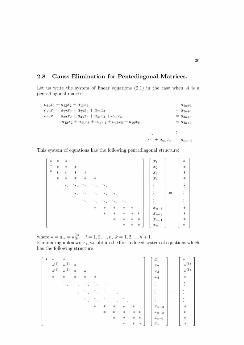
2.8 Gauss Elimination for Pentediagonal Matrices.

Let us write the system of linear equations (2.1) in the case when A is apentadiagonal matrix

a11x1 + a12x2 + a13x3 = a1n+1

a21x1 + a22x2 + a23x3 + a24x4 = a2n+1

a31x1 + a32x2 + a33x3 + a34x4 + a35x5 = a3n+1

a42x2 + a43x3 + a44x4 + a45x5 + a46x6 = a4n+1

. . ....

· · ·+ annxn = ann+1

This system of equations has the following pentadiagonal structure:

∗ ∗ ∗* ∗ ∗ ∗* ∗ ∗ ∗ ∗∗ ∗ ∗ ∗ ∗

. . .. . .

. . .. . .

. . .. . .

. . .. . .

. . .. . .

. . .. . .

. . .. . .

. . .∗ ∗ ∗ ∗ ∗∗ ∗ ∗ ∗ ∗∗ ∗ ∗ ∗∗ ∗ ∗

x1

x2

x3

x4.........xn−3

xn−2

xn−1

xn

=

∗∗∗∗.........∗∗∗∗

where ∗ = aik = a(0)ik , i = 1, 2, ..., n, k = 1, 2, ..., n+ 1.

Eliminating unknown x1, we obtain the first reduced system of equations whichhas the following structure

∗ ∗ ∗∗(1) ∗(1) ∗∗(1) ∗(1) ∗ ∗∗ ∗ ∗ ∗ ∗

. . .. . .

. . .. . .

. . .. . .

. . .. . .

. . .. . .

. . .. . .

. . .. . .

. . .∗ ∗ ∗ ∗ ∗∗ ∗ ∗ ∗ ∗∗ ∗ ∗ ∗∗ ∗ ∗

x1

x2

x3

x4.........xn−3

xn−2

xn−1

xn

=

∗∗(1)∗(1)∗.........∗∗∗∗

40

where

∗(1)ik = aik −mi1a1k, mi1 =ai1

a11, i = 2, 3; k = 2, 3, n+ 1.

After second step of elimination, we obtain the second reduced system ofequations which has the following structure

∗ ∗ ∗∗(1) ∗(1) ∗

∗(2) ∗(2) ∗∗(2) ∗(2) ∗ ∗

. . .. . .

. . .. . .

. . .. . .

. . .. . .

. . .. . .

. . .. . .

. . .. . .

∗ ∗ ∗ ∗ ∗∗ ∗ ∗ ∗ ∗∗ ∗ ∗ ∗∗ ∗ ∗

x1

x2

x3

x4.........xn−3

xn−2

xn−1

xn

=

∗∗(1)∗(2)∗(2).........∗∗∗∗

where

∗(2)ik =

a(1)ik −mi2a

(1)2k , mi2 =

a(1)i2

a(1)22

, i = 3, k = 3, n+ 1,

aik −mi2a2k, mi2 =a

(1)i2

a(1)22

, i = 3, k = 4,

aik −mi2a(1)2k , mi2 =

ai2

a(1)22

, i = 4, k = 3, 4, n+ 1

Continuing elimination of successive unknowns, we obtain the following uppertriangular system of equations:

∗ ∗ ∗∗ (1) ∗ (1) ∗

∗ (2) ∗ (2) ∗∗ (3) ∗ (3) ∗

. . .. . .

. . .. . .

. . .. . .

∗(n−3) ∗(n−3) ∗∗(n−2) ∗(n−2)

∗(n−1)

x1

x2

x3

x4......xn−2

xn−1

xn

=

∗∗(1)∗(2)∗(3)......∗(n−3)

∗(n−2)

∗(n−1)

41

In general, the coefficients are determined by the formulas

∗(s)ik =

a(s−1)ik −misa

(s−1)sk , mis =

a(s−1)is

a(s−1)ss

, i = s+ 1, k = s+ 1, n+ 1,

aik −misask, mis =a

(s−1)is

a(s−1)ss

, i = s+ 1, k = s+ 2,

aik −misa(s−1)sk , mis =

ais

a(s−1)ss

, i = s+ 2, k = s+ 1, s+ 2, n+ 1

for s = 2, 3, ..., n− 2, and for s = n− 1, we have

∗(n−1)nn = a(n−2)

nn −mnn−1a(n−2)n−1n , mnn−1 =

a(n−2)nn−1

a(n−2)n−1n−1

.

and∗(n−1)

nn+1 = a(n−2)nn+1 −mnn−1a

(n−2)n−1n+1.

Hence, by backward substitution, we find the solution

xn =a

(n−1)nn+1

a(n−1)nn

xn−1 =1

a(n−2)n−1n−1

[a(n−2)n−1n+1 − a(n−2)

n−1nxn]

xn−2 =1

a(n−3)n−2n−2

[a(n−3)n−2n+1 − a(n−3)

n−2n−1xn−1 − an−2nxn]

xn−3 =1

a(n−4)n−3n−3

[a(n−4)n−3n+1 − a(n−4)

n−3n−2xn−2 − an−3n−1xn−1]

................................................................................

xs =1

a(s−1)ss

[a(s−1)sn+1 − a(s−1)

ss+1 xs+1 − ass+2xs+2]

.................................................................................

x2 =1

a(1)22

[a(1)2n+1 − a(1)

23 x3 − a24x4]

x1 =1

a11[a1n+1 − a12x2 − a13x3]

(2.39)

The module solvefive in Mathematica solves a system of linear equationswith a pentadiagonal matrix A. The input entries of the pentadiagonal matrixare to be stored on the following list

a = {{a31, a42, ..., ann−1}, {a21, a32, ..., ann−1},{a11, a22, ..., ann}, {a12, a23, ..., an−1n},{a13, a24, ..., an−2,n}, {an+1,1, an+1,2, ..., an+1,n}}.

42

solvefive[a_]:=

Module[{a1,a2,d,a3,a4,f,x,x1,y,n},

{a1,a2,d,a3,a4,f}=Table[a[[i]],{i,1,6}];

n=Length[d];

Do[x=a2[[i-1]]/d[[i-1]];

d[[i]]=d[[i]]-x*a3[[i-1]];

a3[[i]]=a3[[i]]-x*a4[[i-1]];

f[[i]]=f[[i]]-x*f[[i-1]];

x=a1[[i-1]]/d[[i-1]];

a2[[i]]=a2[[i]]-x*a3[[i-1]];

d[[i+1]]=d[[i+1]]-x*a4[[i-1]];

f[[i+1]]=f[[i+1]]-x*f[[i-1]],{i,2,n-1}];

x1=a2[[n-1]]/d[[n-1]];

d[[n]]=d[[n]]-x1*a3[[n-1]];

y[n]=(f[[n]]-x1*f[[n-1]])/d[[n]];

y[n-1]=(f[[n-1]]-a3[[n-1]]*y[n])/d[[n-1]];

y[i_]:=y[i]=

(f[[i]]-a4[[i]]*y[i+2]-a3[[i]]*y[i+1])/d[[i]];

Table[y[i],{i,1,n}]

]

Entering the input data

a={{1.,1.,1.,1.,1.,0.},

{-16.,-16.,-16.,-16.,-16.,-16.,-12.},

{24.,30.,30.,30.,30.,30.,30.,24.},

{-12.,-16.,-16.,-16.,-16.,-16.,-16.},

{0.,1.,1.,1.,1.,1.},

{12.,-1.,0.,0.,0.,0.,-1.,12.}};

we obtain the solution x = {1, 1, 1, 1, 1, 1, 1, 1} by executing the command

solvefive[a].

2.9 Exercises

Question 2.1 Solve the following system of equations:

5x1 + x2 + 2x3 + 5x4 = 110x1 + 2x2 − 6x3 + 9x4 = 43x1 − 2x2 + 4x3 + x4 = 215x1 − 2x2 − x3 + 10x4 = 8

(2.40)

using

1. (a) partial pivoting,

43

(b) full pivoting.

Question 2.2 Using a calculator, solve the following system of equations:

0.000003x1 + 0.001x2 = 610x1 + 3333.333x2 = 19999999

by

1. (a) Gauss elimination without any pivoting,

(b) Gauss elimination with partial pivoting,

(c) Gauss elimination with full pivoting.

Note that the exact solution : x1 = 1000000, x2 = 3000.Explain why Gauss elimination fails to get the accurate solution.

Question 2.3 .(a). Solve the following system of equations:

3x1 + x2 + 2x3 + 3x4 = 106x1 + 4x2 − 6x3 + 9x4 = 259x1 − 6x2 + 4x3 + 8x4 = 2015x1 − 8x2 − x3 + 10x4 = 32

(2.41)

(b). Find LU-decomposition of the matrix

A =

3 1 2 36 4 −6 99 −6 4 815 −8 −1 10

.

Question 2.4 Solve the following system of linear equations by the root squaremethod

4x1 + 2x2 + x3 + x4 = 02x1 + 6x2 + x3 − x4 = 4x1 + x2 + 5x3 + 2x4 = 27x1 − x2 + 2x3 + 7x4 = 19

Question 2.5 .

1. (a) Find the upper-triangular form of the system of linear equations us-ing Gauss elimination method

2x1 + 3x2 − x3 = 1

4x1 + 2x2 + x3 = 2

6x1 + x2 + 4x3 = 7

Solve the above system of equations.

44

(b) Find the LU-decomposition of the matrix

A =

2 3 −14 2 16 1 4

.

Calculate the determinant of the matrix A using the LU-decomposition.

Question 2.6 Consider the following system of equations:

4x1 + x2 = 1x1 + 4x2 + x3 = 4

x2 + 4x3 + x4 = 9· · · · · · · · · · · · · · · · · ·xi−1 + 4xi + xi+1 = i2

· · · · · · · · · · · · · · · · · ·xn−1 + 4xn = n2

Write an algorithm based on Gauss elimination to solve the above system ofequations. Find the solution when n = 10.

Question 2.7 .

Derive the algorithm based on Square Root Method for solving the systemof equations Ax = F , where the tri-diagonal matrix

A =

a b 0 0 0 · · · 0 0

b a b 0 0 · · · 0 0

0 b a b 0 · · · 0 0

· · · · · · · · · · · · · · · · · · · · · · · · a ≥ 2b > 0

0 0 0 0 0 · · · b a

(a)(b) Use the algorithm, which you have found in (a), to solve the system ofequatins

4x1 − x2 = 3

−x1 + 4x2 − x3 = 2

−x2 + 4x3 − x4 = 2

−x3 + 4x4 − x5 = 2

−x4 + 4x5 = 3

45

Question 2.8 .

Consider the system of equations

3x1 − x2 = F1

−x1 + 3x2 − x3 = F2

................ ... .....

−xi−1 + 3xi − xi+1 = Fi, i = 2, 3, ..., n− 1,

................ ... .....

−xn−2 + 3xn−1 − xn = Fn−1

−x4 + 3x5 = Fn

(a)(a) Derive the algorithm based on Gause Elimination Method for solving thesystem of equations and show that the algorithm is numerically stable.

(b) Use the algorithm which you have found in (a) to solve the system ofequatins

3x1 − x2 = 2

−x1 + 3x2 − x3 = 1

−x2 + 3x3 − x4 = 1

−x3 + 3x4 − x5 = 1

−x4 + 3x5 = 2

46

Chapter 3

Eigenvalues and Eigenvectors ofa Matrix

3.1 Eigenvalue Problem

In this chapter, we shall consider the following eigenvalue problem:

Find all real or complex values of λ and corresponding non-zero vectorsx = (x1, x2, . . . , xn)T 6= 0, such that

a11 a12 a13 · · · a1n−1 a1n

a21 a22 a23 · · · a2n−1 a2n

a31 a32 a33 · · · a3n−1 a3n

· · · · · · · · · · · · · · · · · ·an1 an2 an3 · · · ann−1 ann

x1

x2

x3...xn

= λ

x1

x2

x3...xn

. (3.1)

Clearly, this system of equations possesses non-zero solutions if and only if thehomogeneous system of equations

(a11 − λ)x1 + a12x2 + a13x3 + · · ·+ a1nxn = 0a21x1 + (a22 − λ)x2 + a23x3 + · · ·+ a2nxn = 0· · · · · · · · · · · · · · · · · · · · · · · · · · · · · · · · · · · ·an1x1 + an2x2 + an3x3 + · · ·+ (ann − λ)xn = 0

(3.2)

has non-zero solutions. It is well known, the homogeneous system of equations(3.2) has non-zero solutions if and only if the determinant

∆n(λ) =

∣

∣

∣

∣

∣

∣

∣

∣

∣

∣

∣

a11 − λ a12 a13 · · · a1n−1 a1n

a21 a22 − λ a23 · · · a2n−1 a2n

a31 a32 a33 − λ · · · a3n−1 a3n

· · · · · · · · · · · · · · · · · ·an1 an2 an3 · · · ann−1 ann − λ

∣

∣

∣

∣

∣

∣

∣

∣

∣

∣

∣

= 0 (3.3)

47

48

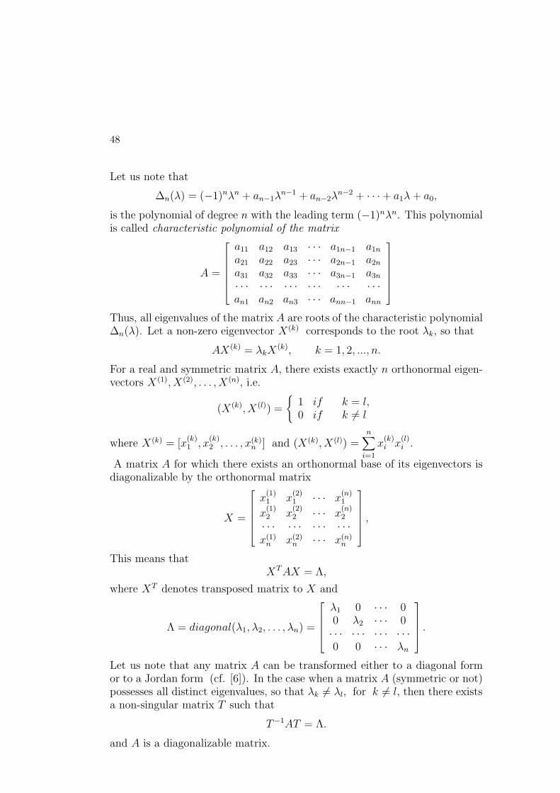
Let us note that

∆n(λ) = (−1)nλn + an−1λn−1 + an−2λ

n−2 + · · ·+ a1λ+ a0,

is the polynomial of degree n with the leading term (−1)nλn. This polynomialis called characteristic polynomial of the matrix

A =

a11 a12 a13 · · · a1n−1 a1n

a21 a22 a23 · · · a2n−1 a2n

a31 a32 a33 · · · a3n−1 a3n

· · · · · · · · · · · · · · · · · ·an1 an2 an3 · · · ann−1 ann

Thus, all eigenvalues of the matrix A are roots of the characteristic polynomial∆n(λ). Let a non-zero eigenvector X(k) corresponds to the root λk, so that

AX(k) = λkX(k), k = 1, 2, ..., n.

For a real and symmetric matrix A, there exists exactly n orthonormal eigen-vectors X(1), X(2), . . . , X(n), i.e.

(X(k), X(l)) =

{

1 if k = l,0 if k 6= l

where X(k) = [x(k)1 , x

(k)2 , . . . , x(k)

n ] and (X(k), X(l)) =n

∑

i=1

x(k)i x

(l)i .

A matrix A for which there exists an orthonormal base of its eigenvectors isdiagonalizable by the orthonormal matrix

X =

x(1)1 x

(2)1 · · · x

(n)1

x(1)2 x

(2)2 · · · x

(n)2

· · · · · · · · · · · ·x(1)

n x(2)n · · · x(n)

n

,

This means thatXTAX = Λ,

where XT denotes transposed matrix to X and

Λ = diagonal(λ1, λ2, . . . , λn) =

λ1 0 · · · 00 λ2 · · · 0· · · · · · · · · · · ·0 0 · · · λn

.

Let us note that any matrix A can be transformed either to a diagonal formor to a Jordan form (cf. [6]). In the case when a matrix A (symmetric or not)possesses all distinct eigenvalues, so that λk 6= λl, for k 6= l, then there existsa non-singular matrix T such that

T−1AT = Λ.

and A is a diagonalizable matrix.

49

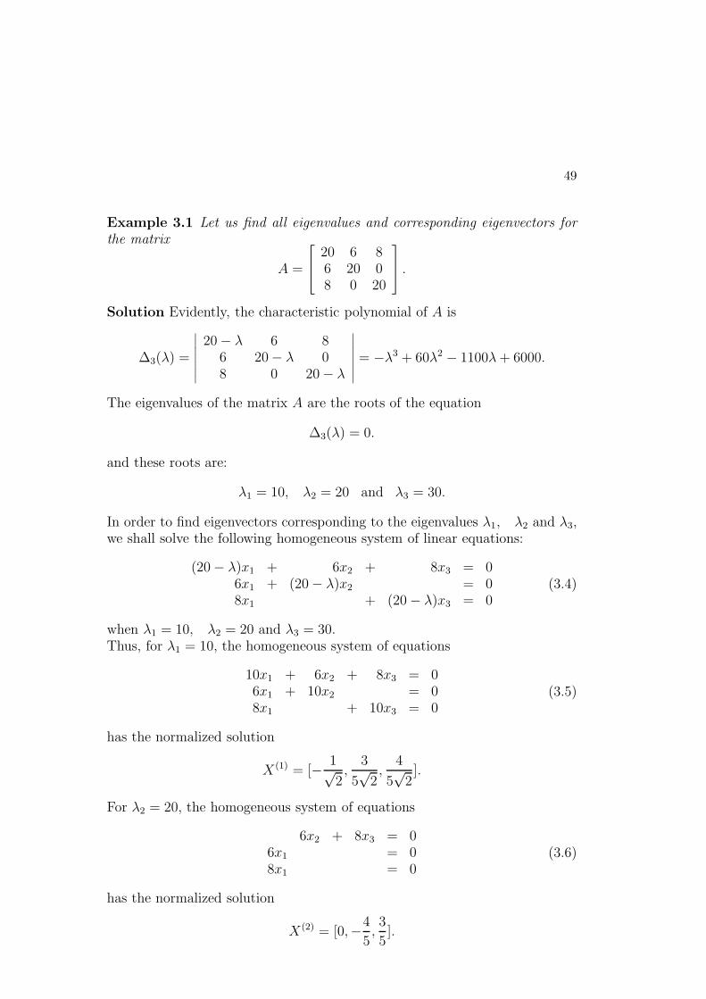
Example 3.1 Let us find all eigenvalues and corresponding eigenvectors forthe matrix

A =

20 6 86 20 08 0 20

.

Solution Evidently, the characteristic polynomial of A is

∆3(λ) =

∣

∣

∣

∣

∣

∣

∣

20− λ 6 86 20− λ 08 0 20− λ

∣

∣

∣

∣

∣

∣

∣

= −λ3 + 60λ2 − 1100λ+ 6000.

The eigenvalues of the matrix A are the roots of the equation

∆3(λ) = 0.

and these roots are:

λ1 = 10, λ2 = 20 and λ3 = 30.

In order to find eigenvectors corresponding to the eigenvalues λ1, λ2 and λ3,we shall solve the following homogeneous system of linear equations:

(20− λ)x1 + 6x2 + 8x3 = 06x1 + (20− λ)x2 = 08x1 + (20− λ)x3 = 0

(3.4)

when λ1 = 10, λ2 = 20 and λ3 = 30.Thus, for λ1 = 10, the homogeneous system of equations

10x1 + 6x2 + 8x3 = 06x1 + 10x2 = 08x1 + 10x3 = 0

(3.5)

has the normalized solution

X(1) = [− 1√2,

3

5√

2,

4

5√

2].

For λ2 = 20, the homogeneous system of equations

6x2 + 8x3 = 06x1 = 08x1 = 0

(3.6)

has the normalized solution

X(2) = [0,−4

5,3

5].

50

For λ3 = 30, the homogeneous system of equations

−10x1 + 6x2 + 8x3 = 06x1 − 10x2 = 08x1 − 10x3 = 0

(3.7)

has the normalized solution

X(3) = [1√2,

3

5√

2,

4

5√

2].

One can check that, X(1), X(2) and X(3) are orthonormal eigenvectors, so that,the orthonormal matrix

X =

− 1√2

01√2

3

5√

2−4

5

3

5√

24

5√

2

3

5

4

5√

2

transforms the matrix A to the following diagonal matrix:

XTAX =

10 0 00 20 00 0 30

= Λ.

Example 3.2 Let us find eigenvalues and eigenvectors of the tri-diagonal ma-trix

A =

2 −1 0 0 · · · 0 0 0−1 2 −1 0 · · · 0 0 00 −1 2 −1 · · · 0 0 0· · · · · · · · · · · · · · · · · · · · · · · ·0 0 0 0 · · · −1 2 −10 0 0 0 · · · 0 −1 2

(n×n)

Solution. The eigenvalues λk and corresponding eigenvectors X(k), k =1, 2, . . . , n, satisfy the following system of linear equations:

2x1 − x2 = λx1

· · · · · · · · · · · · · · · · · ·

−xk−1 + 2xk − xk+1 = λxk

· · · · · · · · · · · · · · · · · ·

−xn−1 + 2xn = λxn

(3.8)

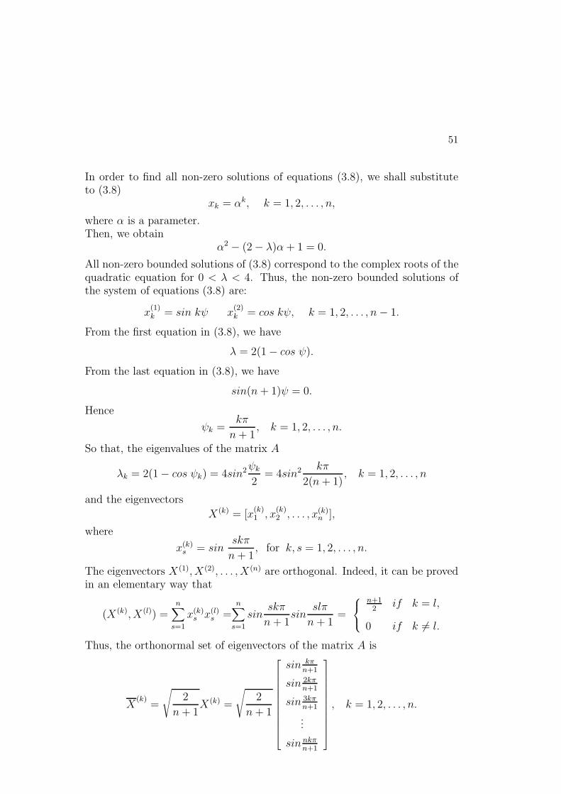
51

In order to find all non-zero solutions of equations (3.8), we shall substituteto (3.8)

xk = αk, k = 1, 2, . . . , n,

where α is a parameter.Then, we obtain

α2 − (2− λ)α + 1 = 0.

All non-zero bounded solutions of (3.8) correspond to the complex roots of thequadratic equation for 0 < λ < 4. Thus, the non-zero bounded solutions ofthe system of equations (3.8) are:

x(1)k = sin kψ x

(2)k = cos kψ, k = 1, 2, . . . , n− 1.

From the first equation in (3.8), we have

λ = 2(1− cos ψ).

From the last equation in (3.8), we have

sin(n+ 1)ψ = 0.

Hence

ψk =kπ

n+ 1, k = 1, 2, . . . , n.

So that, the eigenvalues of the matrix A

λk = 2(1− cos ψk) = 4sin2ψk

2= 4sin2 kπ

2(n+ 1), k = 1, 2, . . . , n

and the eigenvectors

X(k) = [x(k)1 , x

(k)2 , . . . , x(k)

n ],

where

x(k)s = sin

skπ

n+ 1, for k, s = 1, 2, . . . , n.

The eigenvectors X(1), X(2), . . . , X(n) are orthogonal. Indeed, it can be provedin an elementary way that

(X(k), X(l)) =n

∑

s=1

x(k)s x(l)

s =n

∑

s=1

sinskπ

n + 1sin

slπ

n + 1=

n+12

if k = l,

0 if k 6= l.

Thus, the orthonormal set of eigenvectors of the matrix A is

X(k)

=

√

2

n+ 1X(k) =

√

2

n + 1

sin kπn+1

sin 2kπn+1

sin 3kπn+1

...

sin nkπn+1

, k = 1, 2, . . . , n.

52

Let us note that any Hermitian matrix A 1 possesses all real eigenvalues. IfA is a real symmetric matrix then A has also a real orthonormal base ofeigenvectors. Indeed, we have

AX = λX

and the scalarX∗AX = λX∗X.

Since A∗ = A, we get

(X∗AX)∗ = X∗A∗X∗∗ = X∗AX

Then, the scalars X∗X and X∗AX are real. Therefore, λ must be also real.

3.2 Jacobi Method for Real and Symmetric Matrices

The idea of Jacobi method is to find an orthonormal matrix V (i.e. V −1 = V T )such that

V TAV = Λ,

where Λ is a diagonal matrix, V T is transposed matrix to V and V −1 is theinverse matrix to V . As we know, such unitary matrix V exists for any realand symmetric matrix A. Evidently, if A is a diagonal matrix then V = E isa unite matrix. Let A be a non-diagonal matrix. Then, we may choose k andl such that

| akl |= maxi,j=1,2,...,n; i6=j

| aij |> 0.

Now, let us consider the orthogonal matrix

column columnk l↓ ↓

C(1) =

1. . .

1cosψ 0 · · · 0 − sinψ

0 1 · · · 0 0...

. . ....

0 0 · · · 1 0sinψ 0 · · · 0 cosψ

1. . .

1

← rowk

← rowl

k < l

(3.9)

1A is a Hermitian matrix if A∗ = A, where A∗ denotes transposed to A with conjugate entriesof A

53

We can determine the angle ψ in such a way to nullify the entry a(1)kl of the

matrix C(1)TAC(1). Namely, let akl be entry of the matrix AC(1). Then, wefind

akl = − sinψ akk + cosψ akl

all = − sinψ alk + cosψ all

a(1)kl = cosψ akl + sinψ all

(3.10)

Hence, we have

a(1)kl = cosψ(− sinψ akk + cosψ akl) + sinψ(− sinψ akl + cosψ all) =akl((cosψ)2 − (sinψ)2) + cosψ sinψ(all − akk).

and a(1)kl = 0 if the angle ψ satisfies the following equation:

akl(cosψ)2 + (all − akk) cosψ sinψ − akl(sinψ)2 = 0.

So that

akl cos 2ψ − 1

2(akk − all) sin 2ψ = 0.

and

tan2ψ =

2akl

akk − all

if akk 6= all,

∞ if akk = all.

Hence, we get

ψk =

1

2arctan

2akl

akk − all

if akk 6= all,

π

4if akk = all,

We can transform matrix A to an almost diagonal form by the orthogonalmappings C(1), C(2), . . . , C(r). of the form (3.9). Then, we shall show that thesequence of matrices

A(0) = A,A(1) = C(1)TAC(1),A(2) = C(2)TC(1)TAC(1)C(2),· · · · · · · · · · · · · · · · · · · · ·A(r) = C(r)TC(r−1)T . . . C(1)TAC(1)C(2) . . . C(r),· · · · · · · · · · · · · · · · · · · · · · · · · · · · · · · · · · · · · · ·

(3.11)

converges to a diagonal matrix Λ.Indeed, let

A(q) = {a(q)ij }, i, j = 1, 2, . . . , n; q = 0, 1, . . . , r.

The matrices A(q+1), q = 0, 1, . . . , r − 1; are determined by the condition

a(q+1)kq lq

= 0, (3.12)

54

wherea

(q+1)kq lq

= maxi,j=1,2,...,n; i6=j

| a(q)ij | . (3.13)

In order to prove that the sequence (3.11) converges to a diagonal matrix Λ,it is sufficient to show that the non-diagonal entries of A(r) tend to zero whenr →∞, so that

limr→∞

µ(r) = 0,

where

µ(r) =n

∑

i,j=1, i6=j

[a(r)ij ]2. (3.14)

Let

S(A) =n

∑

i,j=1

a2ij .

Then, the following equality holds:

S(A) = Sp(ATA) = Sp(A2)

for a symmetric matrix A, where Sp(A) =n

∑

i=1

aii is the trace of the matrix A.

For two symmetric matrices B and M = ATBA, we have

S(M) = Sp(M2) = Sp((ATBA)2) = Sp(A−1BA) = Sp(B2) = Sp(B). (3.15)

Next, let

A =

[

akk akl

alk all

]

, M =

[

mkk mkl

mlk mll

]

, C =

[

cosψ sinψ−sinψ cosψ

]

.

SinceM = C

TAC,

by (3.15)S(A) = S(M). (3.16)

Also, by (3.15), we obtain

µ(M)− µ(A) = S(M)−n

∑

i=1

mii − [S(A)−n

∑

i=1

a2ii] =

n∑

i=1

a2ii −

n∑

i=1

m2ii.

Hence, we have

mij = aij, for i 6= k, j 6= l, i, j = 1, 2, . . . , n.

Therefore

µ(M)− µ(A) = a2kk + a2

ll −m2kk −m2

ll = S(A)− 2a2kl − S(M) + 2m2

kl.

55

By (3.16), we get equality

µ(M)− µ(A) = 2(m2kl − a2

kl) (3.17)

Now, we shall compute the difference µ(q+1) − µ(q). Namely, by (3.12) and(3.17), we have

µ(q+1) − µ(q) = µ(C(q+1))− µ(C(q)) = 2[(c(q+1)kqlq

)2 − (c(q)kqlq

)2] = −2(c(q)kqlq

)2.

Thereforeµ(q+1) = µ(q) − 2(a

(q)kqlq

)2, q = 0, 1, . . . , r − 1.

Because the entry a(q)kqlq

has been chosen to have the greatest absolute value

(see 3.13), therefore

(a(q)kqlq

)2 ≥ µq

n(n+ 1),

and

µ(q+1) ≤ µ(q) − 2µ(q)

n(n+ 1), q = 0, 1, . . . , r − 1,

Then, we have

0 < µ(r+1) ≤ µ(r)[1− 2

n(n + 1)]r.

Hence, we obtain the limitlimr→∞

µ(r) = 0.

This means that the sequence of matrices (3.11) converges to the diagonalmatrix

Λ =

λ1 0 · · · 00 λ2 · · · 0· · · · · · · · · · · ·0 0 · · · λn

.

The diagonal entries λ1, λ2, . . . , λn are eigenvalues of the matrix A, so that

AV = V Λ,

whereV = lim

r→∞C(0)C(1) · · ·C(r).

Since a product of orthonormal matrices is also an orthonormal matrix, there-fore C(∞) is the orthonormal matrix of eigenvectors of A. In order to stopJacobi iterations, we can use the condition

µ(C(0)C(1) · · ·C(r)) ≤ ǫ,

where ǫ is a given accuracy.

56

Example 3.3 Let us use Jacobi method to find all eigenvalues and eigenvec-tors of the matrix

A =

20 6 86 20 08 0 20

.

Solution . The greatest entry of A out of diagonal

maxi,j=1,2,3; i6=j

| aij |= a13 = 8.

Hence, k = 1, l = 3 and

C(1) =

cosψ 0 −sinψ0 1 0

sinψ 0 cosψ

,

where by (3.10) ψ = π4, since a11 = a33 = 20.

First Jacobi iteration for k = 1, l = 3, a(0)13 = 8 and ψ = 0.785

A(1) = C(1)TAC(1) =

1√2

0 1√2

0 1 0− 1√

20 1√

2

20 6 86 20 08 0 20

1√2

0 − 1√2

0 1 01√2

0 1√2

.

C(1) =

0.707 0.000 −0.7070.000 1.000 0.0000.707 0.000 0.707

,

Hence, we have

A(1) = C(1)TAC(1) =

28.000 4.243 0.0004.243 20.000 −4.2430.000 −4.243 12.000

,

andX(1) X(2) X(3)

V (1) = C(1) =

0.707 0.000 −0.7070.000 1.000 0.0000.707 0.000 0.707

.

Second Jacobi iteration for k = 1, l = 2, a(1)12 = 4.243 and ψ = 0.407

C(2) =

0.918 −0.396 0.0000.396 0.918 0.0000.000 0.000 1.000

,

57

Hence, we have

A(2) = C(2)TA(1)C(2) =

29.831 0.000 −1.6810.000 18.169 −3.895−1.681 −3.895 12.000

.

andX(1) X(2) X(3)

V (2) = C(1)C(2) =

0.649 −0.280 −0.7070.396 0.918 0.0000.649 −0.280 0.707

.

Third Jacobi iteration for k = 2, l = 3, a(2)23 = −3.895 and ψ = −0.451

C(3) =

1.000 0.000 0.0000.000 0.900 0.4350.000 −0.435 0.900

,

Hence, we have

A(3) = C(3)TA(2)C(3) =

29.831 0.732 −1.5130.732 20.053 0.000−1.513 0.000 10.116

,

andX(1) X(2) X(3)

V (3) = C(1)C(2)C(3) =

0.649 0.056 −0.7590.396 0.827 0.4000.649 −0.560 0.515

.

Fourth Jacobi iteration for k = 1, l = 3, a(3)13 = −1.513, and ψ = −0.076

C(4) =

0.997 0.000 0.0760.000 1.000 0.000−0.076 0.000 0.997

,

Hence, we have

A(4) = C(4)TA(3)C(4) =

29.946 0.730 0.0000.730 20.053 0.0560.000 0.056 10.000

,

andX(1) X(2) X(3)

V (4) = C(1)C(2)C(3)C(4) =

0.705 0.056 −0.7070.365 0.827 0.4290.608 −0.560 0.562

.

58

Fifth Jacobi iteration for k = 1, l = 2, a(4)12 = 0.73 and ψ = 0.073

C(5) =

0.997 −0.073 0.0000.073 0.997 0.0000.000 0.000 1.000

,

Hence, we have

A(5) = C(5)TA(4)C(5) =

30.000 0.000 0.0040.000 20.000 0.0560.004 0.056 10.000

,

andX(1) X(2) X(3)

V (5) = C(1)C(2)C(3)C(4)C(5) =

0.707 0.004 −0.7070.424 0.798 0.4290.566 −0.603 0.562

.

Sixth Jacobi iteration for k = 2, l = 3, a(5)23 = 0.056, and ψ = 0.006

C(6) =

1.000 0.000 0.0000.000 1.000 −0.0060.000 0.006 1.000

,

Hence, we have

A(6) = C(6)TA(5)C(6) =

30.000 0.000 0.0040.000 20.000 0.0000.004 0.000 10.000

,

and

X(1) X(2) X(3)

V (6) = C(1)C(2)C(3)C(4)C(5)C(6) =

0.707 0.000 −0.7070.424 0.800 0.4240.566 −0.600 0.566

.

Seventh Jacobi iteration for k = 1, l = 3, a(6)13 = 0.004, and ψ = 0

C(6) =

1.000 0.000 0.0000.000 1.000 0.0000.000 0.000 1.000

,

Hence, we have

A(7) = C(7)TA(6)C(7) =

30.000 0.000 0.0000.000 20.000 0.0000.00 0.000 10.000

,

59

and

X(1) X(2) X(3)

V (7) = C(1)C(2)C(3)C(4)C(5)C(6)C(7) =

0.707 0.000 −0.7070.424 0.800 0.4240.566 −0.600 0.566

.

Finally, the matrix A has the following eigenvalues

λ1 = 30.00λ2 = 20.00λ3 = 10.00

and eigenvectorsX(1) X(2) X(3)

0.707 0.000 −0.7070.424 0.800 0.4240.566 −0.600 0.566

The following module in Mathematica finds eigenvalues and eigenvector of asymmetric matrix a by Jacobi method of iterations

Program 3.1 Mathematica module that solves an eigenvalue problem by iter-ative Jacobi’s method.

jacobi[a_]:=Module[{m,n,ckl,v},

n=Length[a[[1]]]; v=IdentityMatrix[n];m=a;

(* Module ckl finds orthogonal matrix *)

ckl[m_]:=Module[{b,p,k,l,psi,c,s},

b=Abs[m];

Do[b[[i,i]]=0,{i,1,n}];

p=Position[b,Max[b]]; p=First[p];

k=p[[1]]; l=p[[2]];

e=IdentityMatrix[n];

psi=If[m[[k,k]]-m[[l,l]]==0,Pi/4,ArcTan[2*m[[k,l]]/

(m[[k,k]]-m[[l,l]])]/2];

c=N[Cos[psi]]; s=N[Sin[psi]];

e[[k,k]]=c; e[[k,l]]=-s; e[[l,k]]=s; e[[l,l]]=c;

e

];

Do[e=ckl[m];m=Transpose[e].m.e;v=v.e,{7}];

Print["Diagonal matrix of eigenvalues "];

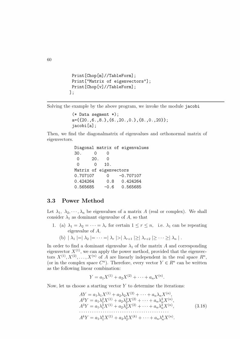
60

Print[Chop[m]//TableForm];

Print["Matrix of eigenvectors"];

Print[Chop[v]//TableForm];

];

Solving the example by the above program, we invoke the module jacobi

(* Data segment *);

a={{20.,6.,8.},{6.,20.,0.},{8.,0.,20}};

jacobi[a];

Then, we find the diagonalmatrix of eigenvalues and orthonormal matrix ofeigenvectors.

Diagonal matrix of eigenvalues

30. 0 0

0 20. 0

0 0 10.

Matrix of eigenvectors

0.707107 0 -0.707107

0.424264 0.8 0.424264

0.565685 -0.6 0.565685

3.3 Power Method

Let λ1, λ2, · · · , λn be eigenvalues of a matrix A (real or complex). We shallconsider λ1 as dominant eigenvalue of A, so that

1. (a) λ1 = λ2 = · · · = λr for certain 1 ≤ r ≤ n, i.e. λ1 can be repeatingeigenvalue of A,

(b) | λ1 |=| λ2 |= · · · =| λr |>| λr+1 |≥| λr+2 |≥ · · · ≥| λn | .In order to find a dominant eigenvalue λ1 of the matrix A and correspondingeigenvector X(1), we can apply the power method, provided that the eigenvec-tors X(1), X(2), . . . , X(n) of A are linearly independent in the real space Rn,(or in the complex space Cn). Therefore, every vector Y ∈ Rn can be writtenas the following linear combination:

Y = a1X(1) + a2X

(2) + · · ·+ anX(n).

Now, let us choose a starting vector Y to determine the iterations:

AY = a1λ1X(1) + a2λ2X

(2) + · · ·+ anλnX(n),

A2Y = a1λ21X

(1) + a2λ22X

(2) + · · ·+ anλ2nX

(n),A3Y = a1λ

31X

(1) + a2λ32X

(2) + · · ·+ anλ2nX

(n),· · · · · · · · · · · · · · · · · · · · · · · · · · · · · · · · · · · · · · · · · ·AkY = a1λ

k1X

(1) + a2λk2X

(k) + · · ·+ anλknX

(n).

(3.18)

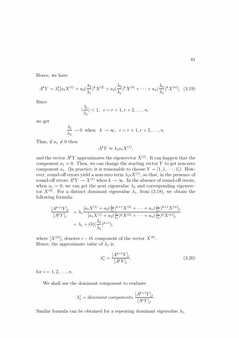
61

Hence, we have

AkY = λk1[a1X

(1) + a2(λ2

λ1)kX(2) + a3(

λ3

λ1)kX(3) + · · ·+ an(

λn

λ1)kX(n)]. (3.19)

Since

|λi

λ1

| < 1, i = r + 1, r + 2, . . . , n,

we getλi

λ1→ 0 when k →∞, i = r + 1, r + 2, . . . , n.

Thus, if a1 6= 0 then

AkY ≈ λ1a1X(1),

and the vector AkY approximates the eigenvector X(1). It can happen that thecomponent a1 = 0. Then, we can change the starting vector Y to get non-zerocomponent a1. (In practice, it is reasonable to choose Y = [1, 1, · · · , 1]). How-ever, round-off errors yield a non-zero term λ1ǫX

(1), so that, in the presence ofround-off errors AkY → X(1) when k →∞. In the absence of round-off errors,when a1 = 0, we can get the next eigenvalue λ2 and corresponding eigenvec-tor X(2). For a distinct dominant eigenvalue λ1, from (3.18), we obtain thefollowing formula:

[Ak+1Y ]i[AkY ]i

= λ1

[a1X(1) + a2(

λ2

λ1

)k+1X(2) + · · ·+ an(λn

λ1

)k+1X(n)]i

[a1X(1) + a2(λ2

λ1

)kX(2) + · · ·+ an(λn

λ1

)kX(n)]i

= λ1 +O((λ2

λ1

)k+1),

where [X(k)]i denotes i− th component of the vector X(k).Hence, the approximate value of λ1 is

λ∗1 =[Ak+1Y ]i[AkY ]i

. (3.20)

for i = 1, 2, . . . , n.

We shall use the dominant component to evaluate

λ∗1 = diminant components[Ak+1Y ]j[AkY ]j

.

Similar formula can be obtained for a repeating dominant eigenvalue λ1.

62

Example 3.4 Let us find the dominant eigenvalue λ1 and corresponding eigen-vector X(1) for the matrix

A =

2 0 31 4 27 0 6

.

using power method.

Solution. One can find, in elementary way, that the eigenvalues and eigen-vectors of A are:

λ1 = 9, λ2 = 4, λ3 = −1

X(1) =

0.3597000.4076610.839309

, X(2) =

010

, X(3) =

−0.70014010.140028

−0.7001401

.

Choosing the starting vector Y = [1, 1, 1], we obtainThe first iteration:

Y1 = AY =

2 0 31 4 27 0 6

.

111

=

5713

.

Thus, the dominant component of Y1 is: λ1 ≈ λ(1)1 = 13

The second iteration:

Y2 = AY1 =

2 0 31 4 27 0 6

.

5713

=

4959113

.

The dominant component of Y2 is : λ1 ≈ λ(2)1 = 9.8

The third iteration:

Y3 = AY2 =

2 0 31 4 27 0 6

.

4959113

=

4375111021

.

The dominant component is : λ1 ≈ λ(3)1 = 9.035399

The fourth iteration :

Y4 = AY3 =

2 0 31 4 27 0 6

.

4375111021

=

393745239185

.

63

The dominant component is: λ1 ≈ λ(4)1 = 9.00915

The fifth iteration :

Y5 = AY4 =

2 0 31 4 27 0 6

.

393745239185

=

354294039982669

.

The dominant component is λ1 ≈ λ(5)1 = 9.00044.

In computations, the scaled power method is used to avoid large numbers.Then, we consider the following vectors as an approximation of X(1):

Yk =AkY

√

[A1Y ]21 + [AkY ]22 + · · ·+ [AkY ]2n, k = 1, 2, . . . ;

The following module in Mathematica finds the dominant eigenvalue and cor-responding eigenvector of a given matrix A.

Program 3.2 Mathematica module that finds a dominant eigenvalue by powermethod.

power[a_,iter_]:=Module[{lambda,n,s,x,vector1,vector2},

n=Length[a];vector2=Table[1,{n}];

Do[{vector1=a.vector2; vector2=a.vector1;

vector3=Table[vector2[[i]]/vector1[[]],{i,1,n}];

lambda=Max[Abs[vector3]];

x=Sqrt[Sum[vector1[[i]]^2,{i,1,n}]];

vector1=vector1/x;

x=Sqrt[Sum[vector2[[i]]^2,{i,1,n}]];

vector2=vector2/x},

{iter}];

Print["Eigenvalue lambda = ",N[lambda,4]];

Print["Eigenvector vector2 = ",vector2];

{lambda,vector2}

]

In order to evaluate the dominant eigenvalue of the matrix

a={{2.,0.,3.},{1.,4.,2.},{7.,0.,6.}};

we enter the number of required iterations iter=3 and execute the commandpower[a,iter] .Then, we obtain the following output

64

Eigenvalue lambda = 9.

Eigenvector vector2 = {0.359539, 0.408585, 0.838922}

{8.99995,{0.35954, 0.40859, 0.83892}}

3.4 The Householder Transformation and Hessenberg

Matrices

Let us state the definition of the Hessenberg matrix

Definition 3.1 A matrix B = {Bij}, i, j = 1, 2, ..., n, is upper Hessenberg ifBij = 0 for i > j + 1, that is, B has the following diagram:

B =

∗ ∗ ∗ · · · ∗ ∗∗ ∗ ∗ · · · ∗ ∗0 ∗ ∗ · · · ∗ ∗...

.... . .

. . ....

...

0 0 0 · · · ∗ ∗0 0 0 · · · ∗ ∗

.

To reduce a matrix A to the Hessenberg matrix B, we apply the Householdertransformation given below.

Definition 3.2 The matrix

H = I − 2x x∗.

is called Householder transformation. 2 where I is n-th order identity matrixand the unitary vector

x =

x1

x2...xn

, x∗ = (x∗1, x∗2, ..., x

∗n) ∈ Cn, ||x||2 =

√x∗x = 1.

Let us note that the Householder transformation is Hermitian orthogonal ma-trix. Indeed, we have

H∗ = I∗ − (2x x∗)∗ = I − 2x x∗ = H,

and

H∗H = H2 = (I − 2x x∗)(I − 2x x∗) = I − 2x x∗ − 2x x∗ + 4x x∗ x x∗ = I,2Householder transformation is also applicable to a matrix with complex entries, then x∗

i meansconjugate to xi, i = 1, 2, ..., n.

65

since x x∗ x x∗ = x x∗.We shall consider the following Householder transformation:

R = I − 2u

||u||2u∗

||u||2, ||u||2 =

√u∗u,

where

u =

x+ ||x||2e1 if x+ ||x||2e1 6= 0,

x− ||x||2e1 if x+ ||x||2e1 = 0,

for any non zero real vector x with components xi, i = 1, 2, ..., n, and e1 =(1, 0, 0, ..., 0)T .The transformation R maps a non zero vector x to the vector ±||x||22e1, thatis

Rx = ±||x||22e1. (3.21)

Indeed, we note that

Rx = x− 2

||u||22uu∗x = x− 2

||u||22(x± ||x||2e1)(x± ||x||2e1)∗x

= x− 2

||u||22(x± ||x||2e1)(||x||22 ± ||x||2x1).

Since||u||22 = (x± ||x||2e1)∗(x± ||x||2e1) = 2(||x||22 ± ||x||2x1),

we have

Rx = x− (x± ||x||2e1) = ±||x||2e1 =

−||x||2e1, x+ ||x||2e1 6= 0,

||x||2e1, x+ ||x||2e1 = 0.

In order to transform a real matrix A = (aij), i, j = 1, 2, ..., n, to the upperHessenberg form B, we apply the following algorithm:Algorithm

1. SetA1 = A, x = (a21, a31, ..., an1)

∗,

u = x± ||x||2e1 =

x+ ||x||2e1 x+ ||x||2e1 6= 0,

x− ||x||2e1 x+ ||x||2e1 = 0.

Rn−1 = In−1 −2

||u||22uu∗,

V1 =

[

I1 00 Rn−1,

]

,

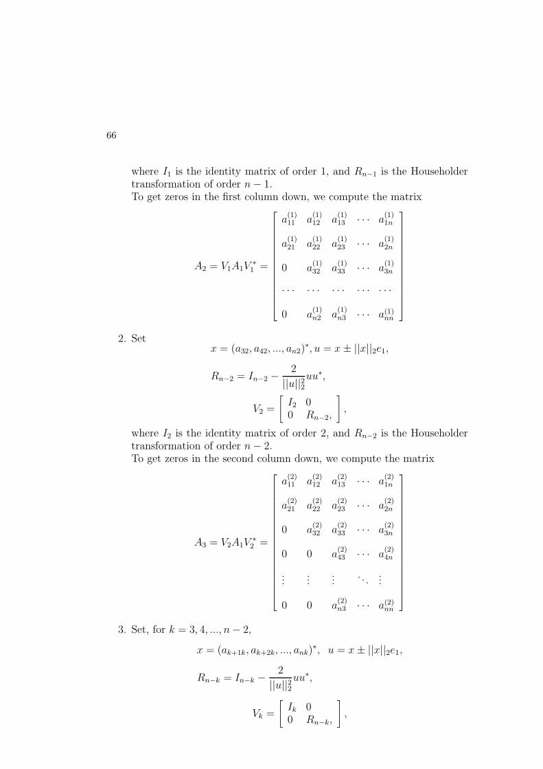
66

where I1 is the identity matrix of order 1, and Rn−1 is the Householdertransformation of order n− 1.To get zeros in the first column down, we compute the matrix

A2 = V1A1V∗1 =

a(1)11 a

(1)12 a

(1)13 · · · a

(1)1n

a(1)21 a

(1)22 a

(1)23 · · · a

(1)2n

0 a(1)32 a

(1)33 · · · a

(1)3n

· · · · · · · · · · · · · · ·

0 a(1)n2 a

(1)n3 · · · a(1)

nn

2. Setx = (a32, a42, ..., an2)

∗, u = x± ||x||2e1,

Rn−2 = In−2 −2

||u||22uu∗,

V2 =

[

I2 00 Rn−2,

]

,

where I2 is the identity matrix of order 2, and Rn−2 is the Householdertransformation of order n− 2.To get zeros in the second column down, we compute the matrix

A3 = V2A1V∗2 =

a(2)11 a

(2)12 a

(2)13 · · · a

(2)1n

a(2)21 a

(2)22 a

(2)23 · · · a

(2)2n

0 a(2)32 a

(2)33 · · · a

(2)3n

0 0 a(2)43 · · · a

(2)4n

......

.... . .

...

0 0 a(2)n3 · · · a(2)

nn

3. Set, for k = 3, 4, ..., n− 2,

x = (ak+1k, ak+2k, ..., ank)∗, u = x± ||x||2e1,

Rn−k = In−k −2

||u||22uu∗,

Vk =

[

Ik 00 Rn−k,

]

,

67

where Ik is the identity matrix of order k, and Rn−k is the Householdertransformation of order n− k.To get zeros in the k-th column down, we compute the matrix

Ak+1 = VkAkV∗k =

a(k)11 a

(k)12 a

(k)13 · · · a

(k)1n−1 a

(k)1n

a(k)21 a

(k)22 a

(k)23 · · · a

(k)2n−1 a

(k)2n

0 a(k)32 a

(k)33 · · · a

(k)3n−1 a

(k)3n

0 0 a(k)43 · · · a

(k)4n−1 a

(k)4n

· · · · · · · · · · · · · · · · · ·

0 0 0 · · · a(k)nn−1 a(k)

nn

Clearly, we get the Hessenberg matrix B = Vn−1An−1V∗n−1.

Example 3.5 Let us reduce the matrix

A =

1 3 4 5−2 2 5 6

1 5 3 72 6 7 4

to the upper Hessenberg form.Following the algorithm, we find

1.

x =

−212

, ||x||2 = 3, u = x+ ||x||2e1 =

112

, ||u||2 = 6,

R3 = I1 −2

||u||2u u∗ =

0.6667 −0.3333 −0.6667−0.3333 0.6667 −0.6667−0.6667 −0.6667 −0.3333

,

V1 =

1.0000 0.0000 0.0000 0.00000.0000 0.6667 −0.3333 −0.66670.0000 −0.3333 0.6667 −0.66670.0000 −0.6667 −0.6667 −0.3333

,

and

A2 = V1 A1V1 =

1.0000 −2.6667 −1.6667 −6.3333−3.0000 −1.4444 0.5556 4.7778

0.0000 0.5556 −2.4444 3.77780.0000 4.7778 3.7778 12.8889

.

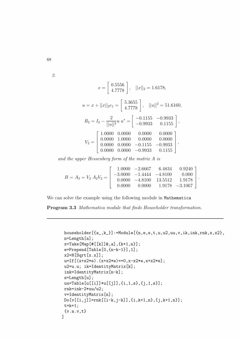
68

2.

x =

[

0.55564.7778

]

, ||x||2 = 1.6178,

u = x+ ||x||2e1 =

[

5.36554.7778

]

, ||u||2 = 51.6160,

R2 = I2 −2

||u||2u u∗ =

[

−0.1155 −0.9933−0.9933 0.1155

]

,

V2 =

1.0000 0.0000 0.0000 0.00000.0000 1.0000 0.0000 0.00000.0000 0.0000 −0.1155 −0.99330.0000 0.0000 −0.9933 0.1155

,

and the upper Hessenberg form of the matrix A is

B = A3 = V2 A2V2 =

1.0000 −2.6667 6.4834 0.9240−3.0000 −1.4444 −4.8100 0.000

0.0000 −4.8100 13.5512 1.91780.0000 0.0000 1.9178 −3.1067

.

We can solve the example using the following module in Mathematica

Program 3.3 Mathematica module that finds Householder transformation.

householder[{a_,k_}]:=Module[{n,e,s,t,u,u2,uu,v,ik,ink,rnk,x,x2},

n=Length[a];

x=Take[Map[#[[k]]&,a],{k+1,n}];

e=Prepend[Table[0,{n-k-1}],1];

x2=N[Sqrt[x.x]];

u=If[(x+x2*e).(x+x2*e)==0,x-x2*e,x+x2*e];

u2=u.u; ik=IdentityMatrix[k];

ink=IdentityMatrix[n-k];

s=Length[u];

uu=Table[u[[i]]*u[[j]],{i,1,s},{j,1,s}];

rnk=ink-2*uu/u2;

v=IdentityMatrix[n];

Do[v[[i,j]]=rnk[[i-k,j-k]],{i,k+1,n},{j,k+1,n}];

t=k+1;

{v.a.v,t}

]

69

To find Hessenberg form of the input data matrix

a={{1.,3.,4.,5.},{-2.,2.,5.,6.},

{1.,5.,3.,7.},{2.,6.,7.,4.}};

we execute the commands

n=4;

b=Nest[householder,{a,1},n-1];

Chop[b[[1]],10^-4]//TableForm

Then, we obtain the following Hessenberg matrix

1. -2.66667 6.48345 -0.924007

-3. -1.44444 -4.80997 0

0 -4.80997 13.5512 -1.91782

0 0 -1.91782 -3.10672

Let us use the Householder transformation for a matrix deflation, that is,to reduce an eigenvalue problem of dimension n to an eigenvalue problem ofdimension n− 1.Matrix Deflation. Let A be a matrix of order n for which an eigenvalue λand an eigenvector x, with the norm ||x||2 = 1, are known. Using the deflation,one can reduce the matrix A to a matrix C of order n− 1, whose eigenvaluesare the same as the remaining eigenvalues of A. To find such a matrix C, weconsider the Householder transformation R of the eigenvector x, so that, by(3.21), we have

Rx = −e1, e1 = (1, 0, ..., 0)T ,

and

x =

x1

x2...xn

= −RT e1 = −

R11

R1,2...R1n

.

Hence, the matrix

RT =

−x1 R21 R31 · · · Rn1

−x2 R22 R32 · · · Rn2

· · · · · · · · · · · · · · ·

−xn R2n R3n · · · Rnn

= [−x, V ],

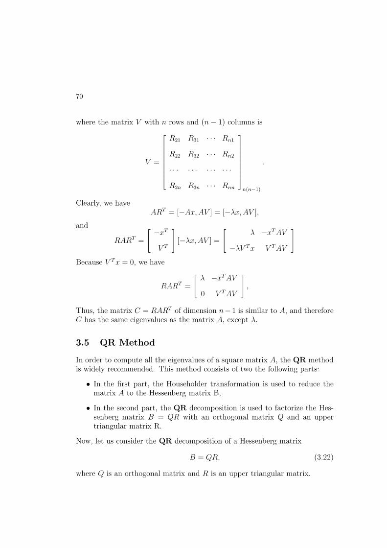
70

where the matrix V with n rows and (n− 1) columns is

V =

R21 R31 · · · Rn1

R22 R32 · · · Rn2

· · · · · · · · · · · ·

R2n R3n · · · Rnn

n(n−1)

.

Clearly, we haveART = [−Ax,AV ] = [−λx,AV ],

and

RART =

−xT

V T

[−λx,AV ] =

λ −xTAV

−λV Tx V TAV

Because V Tx = 0, we have

RART =

λ −xTAV

0 V TAV

,

Thus, the matrix C = RART of dimension n− 1 is similar to A, and thereforeC has the same eigenvalues as the matrix A, except λ.

3.5 QR Method

In order to compute all the eigenvalues of a square matrix A, the QR methodis widely recommended. This method consists of two the following parts:

• In the first part, the Householder transformation is used to reduce thematrix A to the Hessenberg matrix B,

• In the second part, the QR decomposition is used to factorize the Hes-senberg matrix B = QR with an orthogonal matrix Q and an uppertriangular matrix R.

Now, let us consider the QR decomposition of a Hessenberg matrix

B = QR, (3.22)

where Q is an orthogonal matrix and R is an upper triangular matrix.

71

We can obtain such a decomposition, multiplying matrix B by plane rotationmatrices C(2,1), C(3,2), ..., C(n,n−1), where

column columnk l↓ ↓

C(k,l) =

1. . .

1cosψ 0 · · · 0 − sinψ

0 1 · · · 0 0...

. . ....

0 0 · · · 1 0sinψ 0 · · · 0 cosψ

1. . .

1

← rowk

← rowl

k < l

(3.23)Solving the equation

[C(k+1,k)B]k+1,k = Bkk sinψ +Bk+1k cosψ = 0,

we compute the angle

ψ =

Arctan(−Bk+1k

Bkk

), Bkk 6= 0,

π

2, Bkk = 0.

(3.24)

One can show that the multiplication of the Hessenberg matrix B by a planerotation matrix C(k,k−1) preserves the Hessenberg form of the matrix B.Thus, the matrix

R = [C(2,1), C(3,2), ..., C(n,n−1)]B = QTB,

is upper triangular.Hence, we have

B = QR,

where the matrix Q = C(2,1)C(3,2), ..., C(n,n−1), is orthogonal, since the productof orthogonal matrices C(k,k−1), k = 2, 3, ..., n, is also orthogonal.Let us note that the Householder transformation as well as orthogonal planerotation matrices preserve the eigenvalues, so that, the matrices B and R havethe same eigenvalues as the original matrix A. Assuming that the matrix A

72

is reduced to the Hessenberg matrix B, and the decomposition B = QR isknown.Thus, the QR method is given by the following iterative process:The sequence of matrices

A(0), A(1), ..., A(m), ....,

is built according to the following recursive rule:

1. Set A(0) = B,

2. For m = 0, 1, ..., compute the orthogonal matrix

Q(m) = C(2,1)C(3,2), ..., C(n,n−1),

where C(k,k−1) depends on the matrix A(m). This dependence is given,by formula (3.24), to compute the angle ψ.

3. Use the orthogonal matrix Q(m), to find decomposition

A(m) = Q(m)R(m),

with the upper triangular matrix R(m)

4. Compute the matrixA(m+1) = R(m)Q(m).

The matrices A(m), m = 0, 1, ..., are similar to the matrix B. Indeed, we have

A(m+1) = R(m)Q(m) = [Q(m)]−1Q(m)RQ(m) = [Q(m)]−1A(m)Q(m).

Therefore, all the matrices A(m), m = 0, 1, ..., have the same eigenvalues asthe matrix B.Clearly, at m-th iteration, the QR decomposition of the matrix A(m) is neededto compute the next term A(m+1). As we know now, such a decomposition canbe found with use of the orthogonal plane rotation matrices.Thus, we arrive to the following algorithm:

QR Algorithm

Step 1 Transform the matrix

A =

a11 a12 a13 a14 · · · a1n−1 a1n

a21 a22 a23 a24 · · · a2n−1 a2n

a31 a32 a33 a34 · · · a3n−1 a3n

· · · · · · · · · · · · · · · · · · · · · · · ·

an1 an2 an3 an4 · · · ann−1 ann

73

by Householder transformation to the Hessenberg’s matrix

B =

b11 b12 b13 b14 · · · b1n−1 b1n

b21 b22 b23 b24 · · · b2n−1 b2n

0 b32 b33 b34 · · · b3n−1 b3n

0 0 b43 b44 · · · b4n−1 b4n

· · · · · · · · · · · · · · · · · · · · · · · ·

0 0 0 0 · · · bnn−1 bnn

End of step 1.

1. Compute the sequence of matrices

A(0), A(1), A(2), ..., A(m), ...

as follows:

Step 2

(a) Set A(0) = B

(b) Find the QR factorization of the matrix A(0), that is A(0) = Q(0)R(0)

following the scheme

• Compute the angle

ψ =

ArcTan(−A(0)21

A(0)11

), A(0)11 6= 0

π

2, A

(0)11 = 0.

and compute the orthonormal matrix

C(21) =

cosψ −sinψ 0 0 0 · · · 0 0

sinψ cosψ 0 0 · · · 0 0

0 0 1 0 0 · · · 0 0

· · · · · · · · · · · · · · · · · · · · · · · ·

0 0 0 0 0 · · · 0 1

• Compute the matrix A(01) = C(21)A(0) = C(21)B.

To eliminate the element A(0)21 in A(0).

74

• Compute the angle

ψ =

ArcTan(− A(01)32

A(01)22 )

, A(01)22 6= 0

π

2, A

(01)22 = 0.

and compute the orthonormal matrix

C(32) =

1 0 0 0 0 · · · 0 0

0 cosψ −sinψ 0 0 · · · 0 0

0 sinψ cosψ 0 · · · 0 0

0 0 0 1 0 · · · 0 0

· · · · · · · · · · · · · · · · · · · · · · · ·

0 0 0 0 0 · · · 0 1

• Compute the matrix A(11) = C(32)A(01) = C(32)C21)B

To eliminate the element A(01)32 in A(01),

• Compute the angle

ψ =

ArcTan(− A(01)32

A(01)33 )

, A(01)33 6= 0

π

2, A

(01)33 = 0.

and compute the orthonormal matrix

C(43) =

1 0 0 0 0 · · · 0 0

0 1 0 0 0 · · · 0 0

0 0 cosψ − sinψ 0 · · · 0 0

0 0 sinψ cosψ 0 · · · 0 0

· · · · · · · · · · · · · · · · · · · · · · · ·

0 0 0 0 0 · · · 0 1

• Compute the matrix A(21) = C(43)A(01) = C(43)C(32)C21)B

• Continue the process of elimination of the elements A(0)21 , A

(0)32 , A

(0)43 , ..., A

(0)n,n−1

in A(0) to obtain the upper triangular matrix

R(0) = Q(0)A(0)

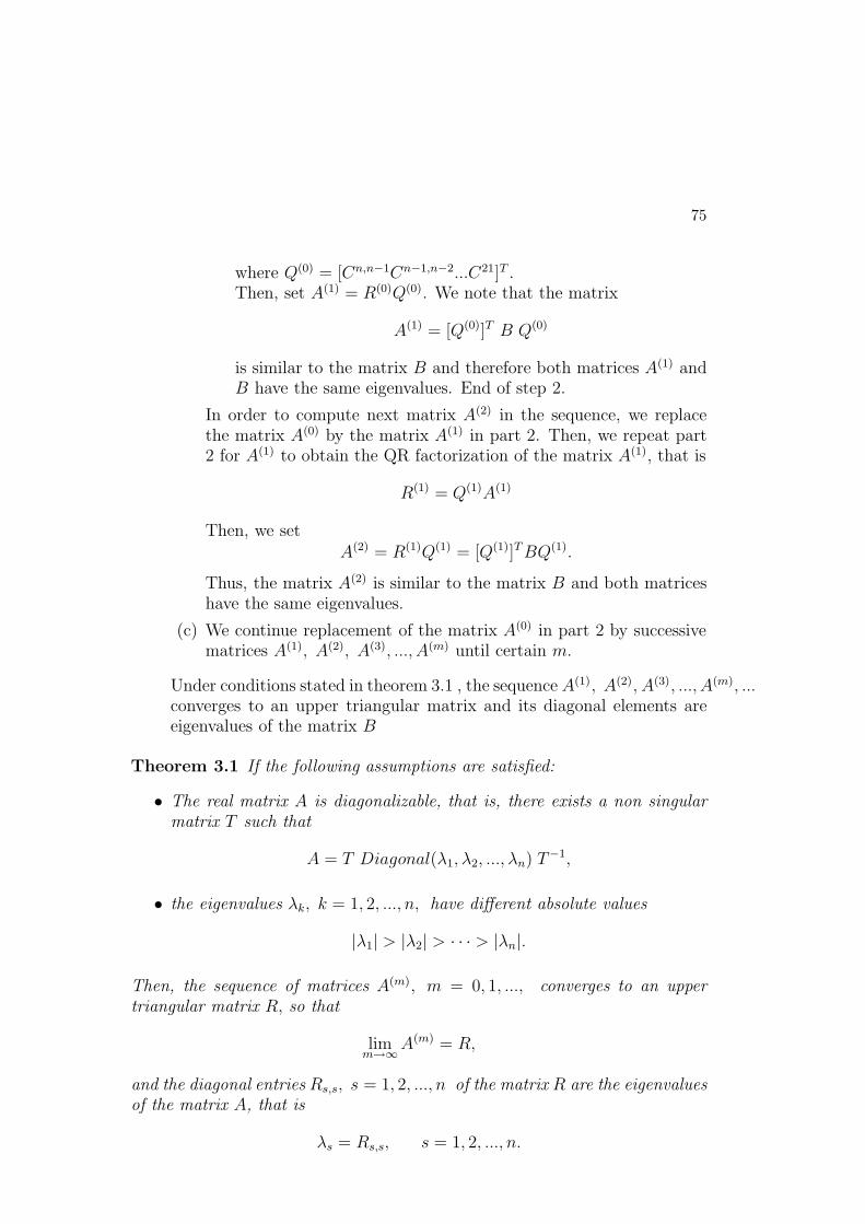
75

where Q(0) = [Cn,n−1Cn−1,n−2...C21]T .Then, set A(1) = R(0)Q(0). We note that the matrix

A(1) = [Q(0)]T B Q(0)

is similar to the matrix B and therefore both matrices A(1) andB have the same eigenvalues. End of step 2.

In order to compute next matrix A(2) in the sequence, we replacethe matrix A(0) by the matrix A(1) in part 2. Then, we repeat part2 for A(1) to obtain the QR factorization of the matrix A(1), that is

R(1) = Q(1)A(1)

Then, we setA(2) = R(1)Q(1) = [Q(1)]TBQ(1).

Thus, the matrix A(2) is similar to the matrix B and both matriceshave the same eigenvalues.

(c) We continue replacement of the matrix A(0) in part 2 by successivematrices A(1), A(2), A(3), ..., A(m) until certain m.

Under conditions stated in theorem 3.1 , the sequence A(1), A(2), A(3), ..., A(m), ...converges to an upper triangular matrix and its diagonal elements areeigenvalues of the matrix B

Theorem 3.1 If the following assumptions are satisfied:

• The real matrix A is diagonalizable, that is, there exists a non singularmatrix T such that

A = T Diagonal(λ1, λ2, ..., λn) T−1,

• the eigenvalues λk, k = 1, 2, ..., n, have different absolute values

|λ1| > |λ2| > · · · > |λn|.

Then, the sequence of matrices A(m), m = 0, 1, ..., converges to an uppertriangular matrix R, so that

limm→∞

A(m) = R,

and the diagonal entries Rs,s, s = 1, 2, ..., n of the matrix R are the eigenvaluesof the matrix A, that is

λs = Rs,s, s = 1, 2, ..., n.

76

In order to accelerate convergence of the sequence A(m), m = 0, 1, ..., one canuse the following algorithm with shiftQR Algorithm with shift. The algorithm with shift is a modification ofthe QR algorithm.Let αm, m = 0, 1, ..., be a sequence of shift numbers. The shift numbersare chosen to accelerate convergence. In the QR algorithm with shift, thesequence of matrices

A(0), A(1), ..., A(m), ...,

is constructed according to the following recursive rule:

1. Set A(0) = B,

2. For m = 0, 1, ..., compute orthogonal matrix Q(m) and upper triangularmatrix R(m), to find the decomposition

A(m) − αmI = Q(m)R(m),

3. Compute the matrix

A(m+1) = R(m)Q(m) + αmI.

If we have an estimate of the eigenvalues λk, k = 1, 2, ..., n we are able to findgood shift numbers.One of a strategy to choose the shift numbers αm, m = 1, 2, ..., is to putαm = A(m)

nn , to get λn, since A(m)ss → λs, s = 1, 2, ..., n, when m→∞.

For a broad range of matrices, the sequence A(0), A(1), ..., A(m), ..., whichis produced by the QR algorithm with shift converges to an upper triangularmatrix R, that is

limm→∞

A(m) = R,

Then, the diagonal entries of the matrix R are eigenvalues of the original ma-trix A.

Example 3.6 Let us apply the QR algorithm to find the eigenvalues of theHessenberg matrix B that is found in the example 1.Thus, we have n = 4, and

B =

0.0000 0.5126 0.4954 −0.7013−5.8523 4.8248 0.7287 −1.3189

0.0000 −0.8535 2.5479 −0.57860.0000 0.0000 −0.4931 2.6273

.

Following the algorithm, we set

A(0) = B,

77

and, we compute the plane rotation matrices:

Since B[1, 1] = 0, we find ψ =π

2and

C(21) =

cosψ − sinψ 0 0sinψ cosψ 0 0

0 0 1 00 0 0 1

=

0 −1 0 01 0 0 00 0 1 00 0 0 1

,

We compute

ψ = Arctan(− [C(2,1)B]21[C(2,1)B]11

= 1.0299

and

C(32) =

1 0 0 00 cosψ − sinψ 00 sinψ cosψ 00 0 0 1

=

1 0 0 00 0.5149 −0.8573 00 0.8573 0.5149 00 0 0 1

,

We compute

ψ = Arctan(− [C(32)C(2,1)B]32[C(32)C(2,1)B]22

= 0.2767

and

C(43) =

1 0 0 00 1 0 00 0 cosψ − sinψ0 0 sinψ cosψ

=

1 0 0 00 0 0 00 0 0.9620 −0.27320 0 0.2732 0.9620

,

The orthogonal matrix

Q(0) = C(21)C(32)C(43) =

0 −1 0 00.5149 0 −0.8573 00.8247 0 0.4953 −0.27320.2342 0 0.1406 0.9620

.

The upper triangular matrix

R(0) = QTB =

5.8523 −4.8248 −0.7287 1.31890 0.9956 −1.9292 0.13490 0 1.8052 −1.58260 0 0 2.2818

,

The matrix

A(1) = R(0)Q(0) =

4.8248 3.6378 4.1050 2.5367−0.9956 1.6538 −0.9924 −0.1415

0 −1.5475 1.3264 −1.26850 0 −0.6233 2.1950

.

78

In order to get the eigenvalues four decimal places accurate, we need to executeabout 30 iterations so that, the final approximate eigenvalues are diagonalentries of the matrix

A(30) = R(29)Q(29) =

4.0000 0.3058 0.5249 5.10080 3.0000 0.0765 3.85280 0 2.0000 2.06460 0 0 1.0000

.

Hence, the eigenvalues λ1 = 1, λ2 = 2, λ3 = 3, and λ4 = 4. These eigenvalues,we can obtain using the following module in Mathematica

Program 3.4 Mathematica module that solves an eigenvalue problem by QRmethod.

rq[a_,iter]:=Module[{rq1,r1},

a1=a;

rq1[a1_]:=Module[{b,n,v,r},

b=a1; n=Length[a1]; v=IdentityMatrix[n];

ckl[{b_,v_,k_}]:=Module[{pa,c,s,e,t,n},

n=Length[b]; e=IdentityMatrix[n];

pa=If[b[[k,k]]==0,Pi/2,ArcTan[-b[[k+1,k]]/b[[k,k]]]];

c=Cos[pa]; s=Sin[pa];

e[[k,k]]=c; e[[k,k+1]]=-s; e[[k+1,k]]=s; e[[k+1,k+1]]=c;

t=k+1;{e.b,e.v,t}

];

r=FixedPoint[ckl,{a1,v,1},n-1];

r[[1]].Transpose[r[[2]]]

];

r1=FixedPoint[rq1,a1,iter]

]

To find the eigenvalues of the Hessenberg matrix

a={{0.0,0.5126,0.4954,-0.7013},

{-5.8523,4.8248,0.7287,-1.3189},

{0.0,-0.8535,2.5479,-0.5786},

{0.0,0.0,-0.4931,2.6273}};

we enter the matrix a, the number of iterations iter=30 and execute thecommands

79

iter=30;

MatrixForm[N[Chop[qr[a,iter],10^-3],4]]

Then, we obtain the following output

4. 0.3058 0.5249 5.101

0 3. 0.07649 3.853

0 0 2. 2.065

0 0 0 1.

3.6 Exercises

Question 3.1 Find all eigenvalues and all orthonormal eigenvectors of thematrix

A =

2 −1 0−1 2 −1

0 −1 2

.

Question 3.2 Find an orthonormal matrix V that transforms the matrix

A =

[

2 31 4

]

to a diagonal form.

Question 3.3 Find all eigenvalues and eigenvectors of the following n × nmatrix:

A =

4 −1 0 0 · · · 0 0 0−1 4 −1 0 · · · 0 0 00 −1 4 −1 · · · 0 0 0· · · · · · · · · · · · · · · · · · · · · · · ·0 0 0 0 · · · −1 4 −10 0 0 0 · · · 0 −1 4

(n×n)

Question 3.4 Solve the following eigenvalue problem:

Ax = λx

by Jacobi method with accuracy ǫ = 0.05, where

A =

2 0 31 4 29 0 6

.

80

Question 3.5 Find the dominant eigenvalue and corresponding eigenvectorof the matrix

A =

5 0 0 30 8 0 00 0 10 0

10 0 0 12

.

Question 3.6 Use the Householder transformation to reduce the followingmatrix to the Hessenberg form:

A =

2 −1 00 2 −13 −1 2

.

Question 3.7 Use the QR method to find all eigenvalues and all orthonormaleigenvectors of the matrix

A =

2 −1 00 2 −13 −1 2

.

Question 3.8 (a) Let

B =

b11 b12 b13

b21 b22 b23

0 b32 b33

be a Hessenberg’s matrix and let A(0), A(1), A(2), ... be the sequence of ma-trices determined by QR factorization of the matrix B. Write the algo-rithm to compute the term A(1) and A(2)

(b) Let the Hessenberg’s matrix

B =

4 0 1

1 2 1

0 1 3

Compute the terms A(0), A(1) and A(2) of the QR sequence A(0), A(1), A(2), ...

Chapter 4

Iterative Methods for Systemsof Linear Equations

4.1 Stationary One Step Linear Methods

In this section, we shall consider a class of one step linear stationary iterativemethods of the following form (cf. [8], [14],[19], [22]):

x(m+1) = Gx(m) + F, m = 0, 1, 2, . . . ; (4.1)

where x(0) is a starting vector, in general, arbitrarily chosen, G is an iterativematrix, and F is a given vector.

Definition 4.1 An iterative method of class (4.1) is said to be consistent withthe system of linear equations

Ax = b, (4.2)

if and only if the exact solution x(d) of the system of equations (4.2) is astationary point of the iterative method i.e.,

x(d) = Gx(d) + F, (4.3)

where the vectors

x =

x1

x2

x3...xn

, b =

b1b2b3...bn

and the matrix

A =

a11 a12 a13 · · · a1n−1 a1n

a21 a22 a23 · · · a2n−1 a2n

a31 a32 a33 · · · a3n−1 a3n

· · · · · · · · · · · · · · · · · ·an1 an2 an3 · · · ann−1 ann

81

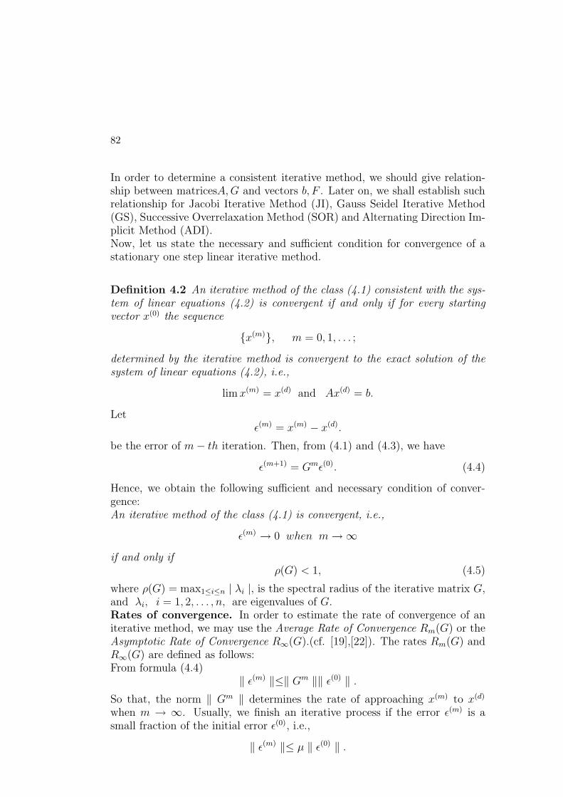
82

In order to determine a consistent iterative method, we should give relation-ship between matricesA,G and vectors b, F . Later on, we shall establish suchrelationship for Jacobi Iterative Method (JI), Gauss Seidel Iterative Method(GS), Successive Overrelaxation Method (SOR) and Alternating Direction Im-plicit Method (ADI).Now, let us state the necessary and sufficient condition for convergence of astationary one step linear iterative method.

Definition 4.2 An iterative method of the class (4.1) consistent with the sys-tem of linear equations (4.2) is convergent if and only if for every startingvector x(0) the sequence

{x(m)}, m = 0, 1, . . . ;

determined by the iterative method is convergent to the exact solution of thesystem of linear equations (4.2), i.e.,

lim x(m) = x(d) and Ax(d) = b.

Letǫ(m) = x(m) − x(d).

be the error of m− th iteration. Then, from (4.1) and (4.3), we have

ǫ(m+1) = Gmǫ(0). (4.4)

Hence, we obtain the following sufficient and necessary condition of conver-gence:An iterative method of the class (4.1) is convergent, i.e.,

ǫ(m) → 0 when m→∞

if and only ifρ(G) < 1, (4.5)

where ρ(G) = max1≤i≤n | λi |, is the spectral radius of the iterative matrix G,and λi, i = 1, 2, . . . , n, are eigenvalues of G.Rates of convergence. In order to estimate the rate of convergence of aniterative method, we may use the Average Rate of Convergence Rm(G) or theAsymptotic Rate of Convergence R∞(G).(cf. [19],[22]). The rates Rm(G) andR∞(G) are defined as follows:From formula (4.4)

‖ ǫ(m) ‖≤‖ Gm ‖‖ ǫ(0) ‖ .So that, the norm ‖ Gm ‖ determines the rate of approaching x(m) to x(d)

when m → ∞. Usually, we finish an iterative process if the error ǫ(m) is asmall fraction of the initial error ǫ(0), i.e.,

‖ ǫ(m) ‖≤ µ ‖ ǫ(0) ‖ .

83

The above inequality holds if

m ≥ − logµ

− 1mlog ‖ Gm ‖ .

Hence, the Average Rate of Convergence is:

Rm(G) = − 1

mlog ‖ Gm ‖,

and the Asymptotic Rate of Convergence is:

R∞(G) = limm→∞

Rm(G) = −logρ(G).

Now, we note that to reduce the initial error µ times

m ≈ − logµ

R∞(G)=

logµ

logρ(G).

iterations are needed.Below, we shall give some of well known stationary one-step iterative methods.

4.2 Jacobi Iterative Method

Let A be a non-singular matrix. and let the diagonal entries aii 6= 0, fori = 1, 2, . . . n. Clearly, the matrix A can be written in the following form:

A = L+D + U,

where the lower-triangular matrix

L =

0 0 0 · · · 0 0a21 0 0 · · · 0 0a31 a32 0 · · · 0 0...

......

. . ....

...an1 an2 an3 · · · ann−1 0

the upper-triangular matrix

U =

0 a12 a13 · · · a1n−1 a1n

0 0 a23 · · · a2n−1 a2n

0 0 0 · · · a3n−1 a3n

......

.... . .

......

0 0 0 · · · 0 0

84

and the diagonal matrix

D =

a11 0 0 · · · 0 00 a22 0 · · · 0 00 0 a33 · · · 0 0...

......

. . ....

...0 0 0 · · · 0 ann

Now, let us write the linear system of equations (4.2) in the following equivalentform:

Dx = −(L+ U)x+ b,

orx = −D−1(L+ U)x+D−1b.

Then, Jacobi iterative method is:

x(m+1) = −D−1(L+ U)x(m) +D−1b, m = 0, 1, . . . ; (4.6)

orx(m+1) = GJx

(m) + FJ , m = 0, 1, . . . ;

where x(0) is the starting vector, GJ = D−1(L+U) is Jacobi’s iterative matrix,and Fj is the following vector FJ = D−1b.In terms of coordinates, Jacobi iterative method takes the following form:

x(m+1)i =

1

aii

n∑

j=1,j 6=i

aijx(m)j +

biaii

,

for i = 1, 2, . . . , n; and m = 0, 1, . . . ;In order to stop Jacobi iterations, we can use the condition

| x(m+1)i − x(m)

i |≤ ǫ, (4.7)

where ǫ is a given accuracy and m is the least integer for which condition (4.7)holds.

Example 4.1 Let us solve the following system of equations

10x1 − x2 − x3 − x4 = 34−x1 + 10x2 − x3 − x4 = 23−x1 − x2 + 10x3 − x4 = 12−x1 − x2 − x3 + 10x4 = 1

by Jacobi iterative method using condition (4.7) to stop the iterations whenǫ = 0.0005.

85

Solution. Let x(0) = (0, 0, 0, 0) be the starting vector. Following Jacobi iter-ations, we findThe first iteration:

x(1)1 = 1

10[34 + x

(0)2 + x

(0)3 + x

(0)4 ] = 3.4

x(1)2 = 1

10[23 + x

(0)1 + x

(0)3 + x

(0)4 ] = 2.3

x(1)3 = 1

10[12 + x

(0)1 + x

(0)2 + x

(0)4 ] = 1.2

x(1)4 = 1

10[1 + x

(0)1 + x

(0)2 + x

(0)3 ] = 0.1

The second iteration:

x(2)1 = 1

10[34 + x

(1)2 + x

(1)3 + x

(1)4 ] = 1

10[34 + 2.3 + 1.2 + 0.1] = 3.76

x(2)2 = 1

10[23 + x

(1)1 + x

(1)3 + x

(1)4 ] = 1

10[23 + 3.4 + 1.2 + 0.1] = 2.77

x(2)3 = 1

10[12 + x

(1)1 + x

(1)2 + x

(1)4 ] = 1

10[12 + 3.4 + 2.3 + 0.1] = 1.78

x(2)4 = 1

10[1 + x

(1)1 + x

(1)2 + x

(1)3 ] = 1

10[1 + 3.4 + 2.3 + 1.2] = 0.79

The third iteration:

x(3)1 = 1

10[34 + x

(2)2 + x

(2)3 + x

(2)4 ] = 1

10[34 + 2.77 + 1.78 + 0.79] = 3.934

x(3)2 = 1

10[23 + x

(2)1 + x

(2)3 + x

(2)4 ] = 1

10[23 + 3.76 + 1.78 + 0.79] = 2.933

x(3)3 = 1

10[12 + x

(2)1 + x

(2)2 + x

(2)4 ] = 1

10[12 + 3.76 + 2.77 + 0.79] = 1.932

x(3)4 = 1

10[1 + x

(2)1 + x

(2)2 + x

(2)3 ] = 1

10[1 + 3.76 + 2.77 + 1.78] = 0.931

The fourth iteration:

x(4)1 = 1

10[34 + x

(3)2 + x

(3)3 + x

(3)4 ] = 1

10[34 + 2.933 + 1.932 + 0.931] = 3.9796

x(4)2 = 1

10[23 + x

(3)1 + x

(3)3 + x

(3)4 ] = 1

10[23 + 3.934 + 1.932 + 0.931] = 2.9797

x(4)3 = 1

10[12 + x

(3)1 + x

(3)2 + x

(3)4 ] = 1

10[12 + 3.3.934 + 2.933 + 0.931] = 1.9798

x(4)4 = 1

10[1 + x

(3)1 + x

(3)2 + x

(3)3 ] = 1

10[1 + 3.934 + 2.933 + 1.932] = 0.9799

We can obtain more accurate approximate solution using the following module

Program 4.1 Mathematica module that solves a linear system of equationsby Jacobi iterative method

86

jacobiItation[a_,x0_]:=Module[{b,d,d1,i,k,l,n,x,u},

n=Length[First[a]]-1;

b=Map[#[[n+1]]&,a];

l=Table[0,{i,1,n},{k,1,n}]; u=l;d=l;

Do[l[[i,k]]=a[[i,k]],{i,2,n},{k,1,i-1}];

Do[u[[i,k]]=a[[i,k]],{i,1,n-1},{k,i+1,n}];

Do[d[[i,i]]=a[[i,i]],{i,1,n}];

d1=Inverse[d];

x=x0;

Do[x=d1.(-(l+u).x+b),{iter}];

x

Entering input data iter=8; and

a={{10.,-1.,-1.,-1.,34.},{-1.,10,-1.,-1.,23.},

{-1.,-1.,10,-1.,12.},{-1.,-1.,-1.,10.,1.}};

x0={0,0,0,0};

we invoke the module

jacobiIteration[a,x0];

Then, we obtain the approximate solution

{3.9999852376, 2.9999852377, 1.9999852378, 0.9999852379}

This solution satisfies the condition (4.7) for m = 7, so that

| x(8)i − x(7)

i |< 0.0003 < ǫ, i = 1, 2, 3, 4.

4.3 Gauss Seidel Iterative Method

Gauss Seidel iterative method is a simple modification of Jacobi iterative

method. Namely, we may use already evaluated x(m+1)j , for j = 1, 2, . . . , i− 1

to determine x(m+1)j , for j = i, i+ 1, . . . , n.

Then, we have

Dx(m+1) = −Lx(m+1) − Ux(m) + b, m = 0, 1, . . . ;

and the Gauss Seidel iterative method takes the following form:

x(m+1) = GSx(m) + FS, m = 0, 1, . . . ; (4.8)

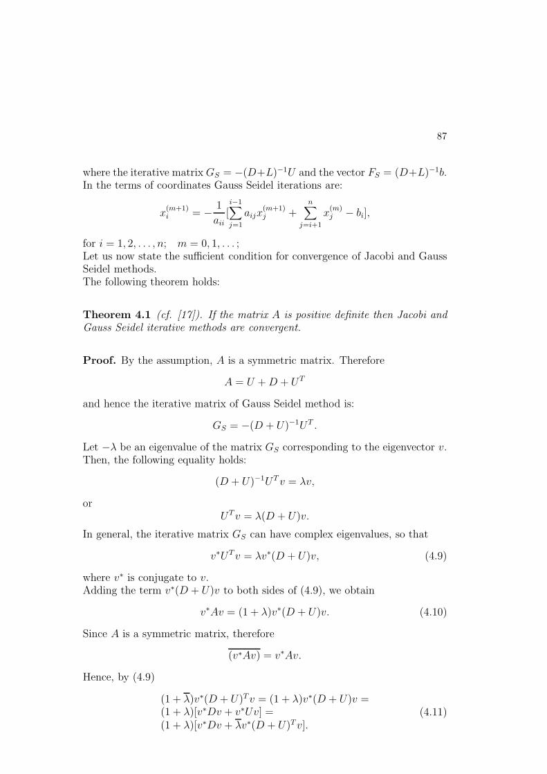
87

where the iterative matrix GS = −(D+L)−1U and the vector FS = (D+L)−1b.In the terms of coordinates Gauss Seidel iterations are:

x(m+1)i = − 1

aii

[i−1∑

j=1

aijx(m+1)j +

n∑

j=i+1

x(m)j − bi],

for i = 1, 2, . . . , n; m = 0, 1, . . . ;Let us now state the sufficient condition for convergence of Jacobi and GaussSeidel methods.The following theorem holds:

Theorem 4.1 (cf. [17]). If the matrix A is positive definite then Jacobi andGauss Seidel iterative methods are convergent.

Proof. By the assumption, A is a symmetric matrix. Therefore

A = U +D + UT

and hence the iterative matrix of Gauss Seidel method is:

GS = −(D + U)−1UT .

Let −λ be an eigenvalue of the matrix GS corresponding to the eigenvector v.Then, the following equality holds:

(D + U)−1UT v = λv,

orUTv = λ(D + U)v.

In general, the iterative matrix GS can have complex eigenvalues, so that

v∗UTv = λv∗(D + U)v, (4.9)

where v∗ is conjugate to v.Adding the term v∗(D + U)v to both sides of (4.9), we obtain

v∗Av = (1 + λ)v∗(D + U)v. (4.10)

Since A is a symmetric matrix, therefore

(v∗Av) = v∗Av.

Hence, by (4.9)

(1 + λ)v∗(D + U)Tv = (1 + λ)v∗(D + U)v =(1 + λ)[v∗Dv + v∗Uv] =(1 + λ)[v∗Dv + λv∗(D + U)Tv].

(4.11)

88

Grouping like terms in (4.11), we arrive at the equality

(1− | λ |2)v∗(D + U)T v = (1 + λ)v∗Dv. (4.12)

Multiplying (4.12) by 1 + λ, we obtain

(1− | λ |2)v∗Av =| 1 + λ |2 v∗Dv. (4.13)

By the assumption, A is a positive definite matrix, thereforeD is also a positivedefinite matrix. Moreover, λ = 1 cannot be an eigenvalue of GS = −(D +U)−1UT since A is a non-singular matrix and v 6= 0 (4.10). Therefore, we have

1− | λ |> 0,

and hence all eigenvalues of GS satisfy the inequality

| λ |< 1.

This means that the spectral radius ρ(GS) < 1. By the necessary and sufficientcondition of convergence, the Gauss Seidel method is convergent.In order to prove that Jacobi method is also convergent, when A is a positivedefinite matrix, we may use the following relations between ρ(GJ) and ρ(GS).

1. (a) ρ(GJ) = ρ(GS) = 0,

(b) ρ(Gj) = ρ(GS) = 1,

(c) ρ(GS) < ρ(GJ ) < 1,

(d) 1 < ρ(GJ) < ρ(GS).

From the above relations, it follows that Jacobi iterative method is convergentif and only if Gauss Seidel method is convergent. One can show that GaussSeidel method is asymptotically twice faster than Jacobi method, i.e.,

R∞(GS) = 2R∞(GJ).

and the number of iterations needed to reduce µ times the initial error ǫ(0) byGauss Seidel iterations is:

m ≈ − logµ

2R∞(GJ).

We can improve the accuracy of the final result of Jacobi iterative and GaussSeidel iterative methods using the following formula:

x∗i = x(m+2)i − (x

(m+2)i − x(m)

i+1)2

x(m+2)i − 2x

m+1)i + x

(m)i

. (4.14)

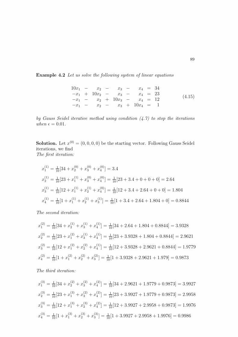
89

Example 4.2 Let us solve the following system of linear equations

10x1 − x2 − x3 − x4 = 34−x1 + 10x2 − x3 − x4 = 23−x1 − x2 + 10x3 − x4 = 12−x1 − x2 − x3 + 10x4 = 1

(4.15)

by Gauss Seidel iterative method using condition (4.7) to stop the iterationswhen ǫ = 0.01.

Solution. Let x(0) = (0, 0, 0, 0) be the starting vector. Following Gauss Seideliterations, we findThe first iteration:

x(1)1 = 1

10[34 + x

(0)2 + x

(0)3 + x

(0)4 ] = 3.4

x(1)2 = 1

10[23 + x

(1)1 + x

(0)3 + x

(0)4 ] = 1

10[23 + 3.4 + 0 + 0 + 0] = 2.64

x(1)3 = 1

10[12 + x

(1)1 + x

(1)2 + x

(0)4 ] = 1

10[12 + 3.4 + 2.64 + 0 + 0] = 1.804

x(1)4 = 1

10[1 + x

(1)1 + x

(1)2 + x

(1)3 ] = 1

10[1 + 3.4 + 2.64 + 1.804 + 0] = 0.8844

The second iteration:

x(2)1 = 1

10[34 + x

(1)2 + x

(1)3 + x

(1)4 ] = 1

10[34 + 2.64 + 1.804 + 0.8844] = 3.9328

x(2)2 = 1

10[23 + x

(2)1 + x

(1)3 + x

(1)4 ] = 1

10[23 + 3.9328 + 1.804 + 0.8844] = 2.9621

x(2)3 = 1

10[12 + x

(2)1 + x

(2)2 + x

(1)4 ] = 1

10[12 + 3.9328 + 2.9621 + 0.8844] = 1.9779

x(2)4 = 1

10[1 + x

(2)1 + x

(2)2 + x

(2)3 ] = 1

10[1 + 3.9328 + 2.9621 + 1.979] = 0.9873

The third iteration:

x(3)1 = 1

10[34 + x

(2)2 + x

(2)3 + x

(2)4 ] = 1

10[34 + 2.9621 + 1.9779 + 0.9873] = 3.9927

x(3)2 = 1

10[23 + x

(3)1 + x

(2)3 + x

(2)4 ] = 1

10[23 + 3.9927 + 1.9779 + 0.9873] = 2.9958

x(3)3 = 1

10[12 + x

(3)1 + x

(3)2 + x

(2)4 ] = 1

10[12 + 3.9927 + 2.9958 + 0.9873] = 1.9976

x(3)4 = 1

10[1 + x

(3)1 + x

(3)2 + x

(3)3 ] = 1

10[1 + 3.9927 + 2.9958 + 1.9976] = 0.9986

90

The fourth iteration:

x(4)1 = 1

10[34 + x

(3)2 + x

(3)3 + x

(3)4 ] = 1

10[34 + 2.9958 + 1.9976 + 0.9986] = 3.9992

x(4)2 = 1

10[23 + x

(4)1 + x

(3)3 + x

(3)4 ] = 1

10[23 + 3.9992 + 1.9976 + 0.9986] = 2.9995

x(4)3 = 1

10[12 + x

(4)1 + x

(4)2 + x

(3)4 ] = 1

10[12 + 3.9992 + 2.9995 + 0.9986] = 1.9997

x(4)4 = 1

10[1 + x

(4)1 + x

(4)2 + x

(4)3 ] = 1

10[1 + 3.9992 + 2.9995 + 1.9997] = 0.9998

Evidently, condition (4.7) is satisfied for m = 3, so that

| x(4)i − x(3)

i |≤ 0.008 < ǫ, i = 1, 2, 3, 4.

We can solve a system of linear equations by Gauss Seidel method of iterationsusing the following Mathematica module:

Program 4.2 Mathematica module that solves a linear system of equationsby Gauss Seidel iterative method

gaussSeidel[a_,x0_]:=Module[{b,d,d1,i,k,l,n,x,u},

n=Length[a[[1]]]-1;

b=Map[#[[n+1]]&,a];

l=Table[0,{i,1,n},{k,1,n}]; u=l;d=l;

Do[l[[i,k]]=a[[i,k]],{i,2,n},{k,1,i-1}];

Do[u[[i,k]]=a[[i,k]],{i,1,n-1},{k,i+1,n}];

Do[d[[i,i]]=a[[i,i]],{i,1,n}];

d1=Inverse[d+l];

x=x0;

Do[x=d1.(-u.x+b),{4}];

x

];

In order to repeat the solution of the above example, using the module seidel,we enter input data matrix and the starting vector

a={{10.,-1.,-1.,-1.,34.},{-1.,10,-1.,-1.,23.},

{-1.,-1.,10,-1.,12.},{-1.,-1.,-1.,10.,1.}};

x0={0,0,0,0};

Then, we execute the instruction

N[gaussSeidel[a,x0],4]

91

to obtain the approximate solution 3.999, 3., 2., 0.9998.

Let us note that, we have got the same numerical solution of the system ofequations (4.15) by Gauss Seidel iterative method for four iterations, and byJacobi iterative method for 8 iterations. Still, we can improve the results usingformula (4.14). Namely, we obtain the four digit accurate solution using onlythree iterations: the second, the third and the fourth, i.e.,

x(∗)1 = x

(4)1 −

[x(4)1 − x(3)

1 ]2

x(4)1 − 2x

(3)1 + x

(2)1

= 3.9992− [3.9992− 3.9927]2

3.9992− 2 ∗ 3.9927 + 3.9328= 4.0000

x(∗)2 = x

(4)2 −

[x(4)2 − x(3)

2 ]2

x(4)2 − 2x

(3)2 + x

(2)2

= 2.9995− (2.9995− 2.9958)2

2.9995− 2 ∗ 2.9958 + 2.9621= 3.0000

x(∗)3 = x

(4)3 −

[x(4)3 − x(3)

3 ]2

x(4)3 − 2x

(3)3 + x

(2)3

= 1.9997− (1.9997− 1.9976)2

1.9997− 2 ∗ 1.9976 + 1.9779= 2.0000

x(∗)4 = x

(4)4 −

[x(4)4 − x(3)

4 ]2

x(4)4 − 2x

(3)4 + x

(2)4

= 0.9998− (0.9998− 0.9986)2

0.9998− 2 ∗ 0.9986 + 0.9873= 1.0000

4.4 Successive Overrelaxation Method (SOR)

Let us rewrite the system of equations (4.2) in the following form:

x = (−D−1L−D−1U)x+D−1b. (4.16)

Then, the successive overrelaxation iterations take the following form:

x(m+1) = w[−D−1Lx(m+1) −D−1Ux(m) +D−1b] + (1− w)x(m),m = 0, 1, . . . ;

(4.17)

where w is a parameter, x(0) is a starting vector.In terms of coordinates, SOR iterations are:

x(m+1)i = −w[

i−1∑

j=1

aij

aii

x(m+1)j +

n∑

j=i+1

aij

aii

x(m)j − bi

aii

] + (1− w)x(m)i , (4.18)

i = 1, 2, . . . ; m = 0, 1, . . . ;Clearly, SOR method is one step linear stationary method, since from (4.17),we get

x(m+1) = Gwx(m) + Fw, m = 0, 1, . . . ; (4.19)

where the iterative matrix

Gw = (E + wD−1L)−1[(1− w)E − wD−1U ]

and the vectorFw = wD−1b

92

.Let us note that for w = 1, SOR iterations (4.19) are the same as Gauss Seideliterations (4.8). The rate of convergence of SOR method depends on the valueof the parameter w. Naturally, the fastest convergence of SOR iterations willbe for optimal value of w = wopt for which the spectral radius ρ(Gw) attainsits minimum. The optimal value of the parameter w can be determined by thefollowing formula (cf. [22]):

wopt =2

1 +√

1− ρ2(GJ), (4.20)

where ρ(GJ) is the spectral the matrix GJ .The conditions of convergence of SOR method are given in the following the-orem:

Theorem 4.2 Let A be a symmetric matrix with the positive diagonal entriesaii > 0, i = 1, 2, . . . ; Then, SOR method converges if and only if A is apositive definite matrix and 0 < w < 2.

Thus, SOR method as well as Jacobi and Gauss Seidel methods are convergentfor positive definite matrices. Among them SOR method has the greatest rateof convergence, i.e.,

R∞(Gwopt) = 2

√

R∞(GJ),

where R∞(GJ) is the asymptotic rate of convergence of Jacobi method. How-ever, in order to use SOR method with the optimal parameter wopt, we have toknow the radius of convergence ρ(GJ ) of Jacobi method. In some interestingcases (for example when approximating elliptic equations), ρ(GJ) is knownand then, we may apply SOR method successfully.

Example 4.3 Let us solve the following system of linear equations

10x1 − x2 − x3 − x4 = 34−x1 + 10x2 − x3 − x4 = 23−x1 − x2 + 10x3 − x4 = 12−x1 − x2 − x3 + 10x4 = 1

by SOR method using condition (4.7) to stop the iterations when ǫ = 0.05.

Solution. One can find that the spectral radius ρ(GJ) = 0.3, where Jacobiiterative matrix

GJ = E −D−1A =

1 0 0 00 1 0 00 0 1 00 0 0 1

− 1

10

10 −1 −1 −1−1 10 −1 −1−1 −1 10 −1−1 −1 −1 10

=

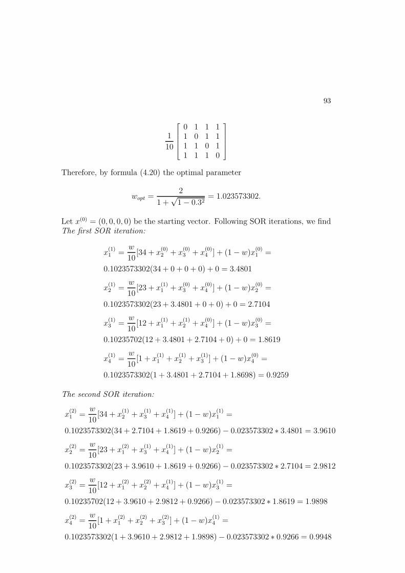
93

1

10

0 1 1 11 0 1 11 1 0 11 1 1 0

Therefore, by formula (4.20) the optimal parameter

wopt =2

1 +√

1− 0.32= 1.023573302.

Let x(0) = (0, 0, 0, 0) be the starting vector. Following SOR iterations, we findThe first SOR iteration:

x(1)1 =

w

10[34 + x

(0)2 + x

(0)3 + x

(0)4 ] + (1− w)x

(0)1 =

0.1023573302(34 + 0 + 0 + 0) + 0 = 3.4801

x(1)2 =

w

10[23 + x

(1)1 + x

(0)3 + x

(0)4 ] + (1− w)x

(0)2 =

0.1023573302(23 + 3.4801 + 0 + 0) + 0 = 2.7104

x(1)3 =

w

10[12 + x

(1)1 + x

(1)2 + x

(0)4 ] + (1− w)x

(0)3 =

0.10235702(12 + 3.4801 + 2.7104 + 0) + 0 = 1.8619

x(1)4 =

w

10[1 + x

(1)1 + x

(1)2 + x

(1)3 ] + (1− w)x

(0)4 =

0.1023573302(1 + 3.4801 + 2.7104 + 1.8698) = 0.9259

The second SOR iteration:

x(2)1 =

w

10[34 + x

(1)2 + x

(1)3 + x

(1)4 ] + (1− w)x

(1)1 =

0.1023573302(34 + 2.7104 + 1.8619 + 0.9266)− 0.023573302 ∗ 3.4801 = 3.9610

x(2)2 =

w

10[23 + x

(2)1 + x

(1)3 + x

(1)4 ] + (1− w)x

(1)2 =

0.1023573302(23 + 3.9610 + 1.8619 + 0.9266)− 0.023573302 ∗ 2.7104 = 2.9812

x(2)3 =

w

10[12 + x

(2)1 + x

(2)2 + x

(1)4 ] + (1− w)x

(1)3 =

0.10235702(12 + 3.9610 + 2.9812 + 0.9266)− 0.023573302 ∗ 1.8619 = 1.9898

x(2)4 =

w

10[1 + x

(2)1 + x

(2)2 + x

(2)3 ] + (1− w)x

(1)4 =

0.1023573302(1 + 3.9610 + 2.9812 + 1.9898)− 0.023573302 ∗ 0.9266 = 0.9948

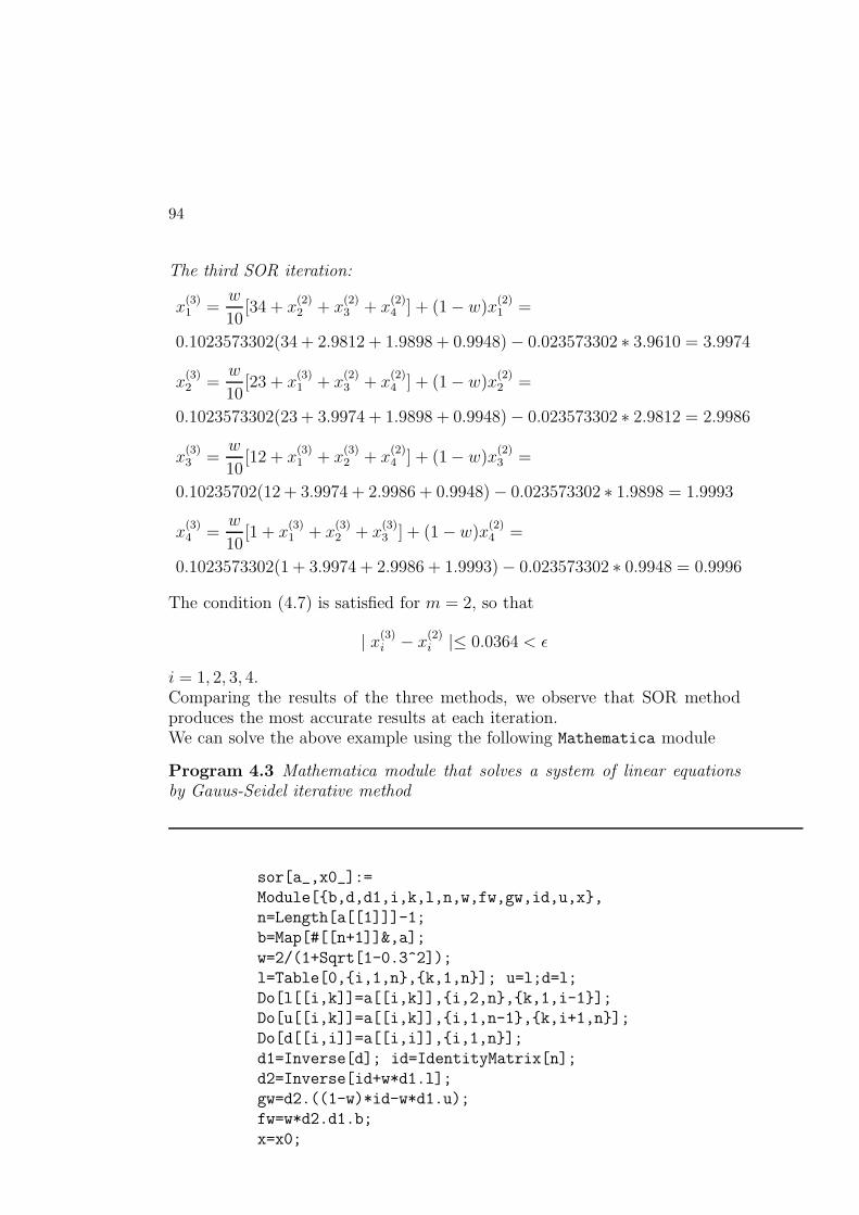
94

The third SOR iteration:

x(3)1 =

w

10[34 + x

(2)2 + x

(2)3 + x

(2)4 ] + (1− w)x

(2)1 =

0.1023573302(34 + 2.9812 + 1.9898 + 0.9948)− 0.023573302 ∗ 3.9610 = 3.9974

x(3)2 =

w

10[23 + x

(3)1 + x

(2)3 + x

(2)4 ] + (1− w)x

(2)2 =

0.1023573302(23 + 3.9974 + 1.9898 + 0.9948)− 0.023573302 ∗ 2.9812 = 2.9986

x(3)3 =

w

10[12 + x

(3)1 + x

(3)2 + x

(2)4 ] + (1− w)x

(2)3 =

0.10235702(12 + 3.9974 + 2.9986 + 0.9948)− 0.023573302 ∗ 1.9898 = 1.9993

x(3)4 =

w

10[1 + x

(3)1 + x

(3)2 + x

(3)3 ] + (1− w)x

(2)4 =

0.1023573302(1 + 3.9974 + 2.9986 + 1.9993)− 0.023573302 ∗ 0.9948 = 0.9996

The condition (4.7) is satisfied for m = 2, so that

| x(3)i − x(2)

i |≤ 0.0364 < ǫ

i = 1, 2, 3, 4.Comparing the results of the three methods, we observe that SOR methodproduces the most accurate results at each iteration.We can solve the above example using the following Mathematica module

Program 4.3 Mathematica module that solves a system of linear equationsby Gauus-Seidel iterative method

sor[a_,x0_]:=

Module[{b,d,d1,i,k,l,n,w,fw,gw,id,u,x},

n=Length[a[[1]]]-1;

b=Map[#[[n+1]]&,a];

w=2/(1+Sqrt[1-0.3^2]);

l=Table[0,{i,1,n},{k,1,n}]; u=l;d=l;

Do[l[[i,k]]=a[[i,k]],{i,2,n},{k,1,i-1}];

Do[u[[i,k]]=a[[i,k]],{i,1,n-1},{k,i+1,n}];

Do[d[[i,i]]=a[[i,i]],{i,1,n}];

d1=Inverse[d]; id=IdentityMatrix[n];

d2=Inverse[id+w*d1.l];

gw=d2.((1-w)*id-w*d1.u);

fw=w*d2.d1.b;

x=x0;

95

Do[x=gw.x+fw,{3}];

x

];

Entering data matrix a and starting vector x0

a={{10.,-1.,-1.,-1.,34.},{-1.,10,-1.,-1.,23.},

{-1.,-1.,10,-1.,12.},{-1.,-1.,-1.,10.,1.}};

x0={0,0,0,0};

we obtain the approximate solution 3.9974, 2.9986, 1.9993, 0.99964, by exe-cution of the command N[sor[a,x0],5].

4.5 Alternating Direction Implicit Method (ADI)

The ADI iterative method in its first version was published by D.W. Peacemanand H.H. Rachford in 1955. Here, we shall present a stationary variant of ADImethod, (cf. [22]).1 Let us assume that A is a positive definite matrix. We split A in threecomponents as follows:

A = L+D + U,

where D is diagonal matrix.By ADI method, the sequence {x(m)}, m = 0, 1, . . . ; of successive iterationsis determined in two steps. Namely, for a given vector x(m) the next two termsx(m+ 1

2) and x(m+1) are computed by the following recursive formulas:

(L1 + βE)x(m+ 1

2) = b− (U1 − βE)x(m),

(U1 + βE)x(m+1) = b− (L1 − βE)x(m+ 1

2), m = 0, 1, ...;

(4.21)

where L1 = L+ 12D, U1 = U + 1

2D, and β is a parameter.

Eliminating x(m+ 1

2) from equations (4.21), we obtain

x(m+1) = G(A, β)x(m) + F (A, β), m = 0, 1, ...;

where the iterative matrix of ADI method

G(A, β) = (U1 + βE)−1(L1 − βE)(L1 + βE)−1(U1 − βE),

and the vector

F (A, β) = (U1 + βE)−1b− (U1 + βE)−1(L1 − βE)−1(L1 + βE)−1b.

1See a broad description of ADI method in [19], [22]

96

Thus, ADI method is also one step stationary method, and it is convergent ifthe spectral radius ρ(G(A, β)) < 1.On the other hand, the spectral radius

ρ(G(A, β)) = max1≤k≤n

[λk − βλk + β

]2,

where λk is the eigenvalue of the matrix L1, and

[λk − βλk + β

]2

is the eigenvalue of the iterative matrix G(A, β).By the assumption, A is a positive definite matrix. Therefore, L1 and U1 arealso a positive definite matrices and all their eigenvalues are positive, so that

0 < a ≤ λk ≤ b, k = 1, 2, ..., n;

Then, the spectral radiusρ(G(A, β)) < 1

for every β > 0. Therefore ADI method is convergent for every β > 0.In order to reach the greatest rate of convergence, we can choose an optimalvalue of the parameter β to obtain the smallest value of ρ(G(A, β)). Thus, weshall find such βopt for which

ρ(A, βopt) = minβ>0

maxa≤λ≤b

[λ− βλ+ β

]2.

One can find that

maxa≤λ≤b

|λ− βλ+ β

| = max{β − aβ + a

,b− βb+ β

} =

b− βb+ β

if a ≤ β ≤√ab,

β − aβ + a

if√ab ≤ β ≤ b.

Hence, the optimal value of parameter βopt =√ab.

Example 4.4 Let us solve the following system of linear equations:

10x1 − x2 − x3 − x4 = 34−x1 + 10x2 − x3 − x4 = 23−x1 − x2 + 10x3 − x4 = 12−x1 − x2 − x3 + 10x4 = 1

by ADI method using condition (4.7) to stop the iterations when ǫ = 0.005.

97

Solution. Let us note that the matrix

A =

10 −1 −1 −1−1 10 −1 −1−1 −1 10 −1−1 −1 −1 10

can be written as follows:A = L+D + U,

where

L =

4 −1 0 0−1 4 −1 0

0 −1 4 −10 0 −1 4

, D =

2 0 0 00 2 0 00 0 2 00 0 0 2

,

U =

4 0 −1 −10 4 0 −1−1 0 4 0−1 −1 0 4

.

Evidently, the matrices L, D and U satisfy conditions (a) and (b) and theassumptions of theorem 1. Therefore, ADI method (4.21) is convergent. Inthe example, we shall use the optimal value of the parameters when

βopt = βopt =√ab

Namely, one can find that the matrices

L1 == L+1

2D =

5 −1 0 0−1 5 −1 0

0 −1 5 −10 0 −1 5

U1 == U +1

2D =

5 0 −1 −10 5 0 −1−1 0 5 0−1 −1 0 5

have the same eigenvalues

ν1 = λ1 = 3.381966, ν2 = λ2 = 4.381966,

ν3 = λ3 = 5.618033, ν4 = λ4 = 6.618033.

Hence a = 3.381966, b = 6.6180340 and βopt =√ab = 4.7309579.

Let x(0) = (0, 0, 0, 0) be the starting vector. Following ADI iterations (4.21),we arrive at the following results:

98

ADI Iterationsx(m) x1 x2 x3 x4

x(0) 0.0000 0.0000 0.0000 0.0000x(0.5) 3.7934 2.9137 1.5596 0.2630x(1) 3.9858 2.9325 1.9261 0.9667x(1.5) 3.9891 2.9972 1.9995 0.9924x(2) 3.9999 2.9989 1.9990 1.0000

The error : max[x(2)i − x(0)

i ] = 0.0011

.

Let us note that ADI method produces the most accurate results at eachiteration as compared with the other methods (Jacobi, GS, SOR). However,ADI method converges well when optimal parameters are used. Then, twolinear systems of equations have to be solved at each iteration. This makesADI method less effective. Although, in some cases when the matrices L1 andU1 have simple structure (for instance, L1 and U1 are tri-diagonal matrices),ADI method can produce a satisfactory solution using relatively small numberof arithmetic operations. In order to reduce the initial error µ times

m ≈ log(µ)

log(ρ(GA))

arithmetic operations are needed.

4.6 Conjugate Gradient Method (CG)

The conjugate gradient method is applicable to a linear system of n equations

Ax = b, (4.22)

with a positive definite matrix A.This method produces a solution of the system (4.22) in at most n iterations,provided that computations are done in exact arithmetic. An implementationof the method on a computer may affect infinite iterative process.The method is based on a set v(1) , v(2) , ..., v(n) of A-orthogonal vectors in thesense of the following inner product

(Av(i), v(j)) =n

∑

k=1

n∑

s=1

aksv(i)k v(j)

s ,

where the vector v(i) = (v(i)1 , v

(i)2 , . . . , v(i)

n ) is in the real space Rn. So that

(Av(i), v(j)) =

1, i = j,

0, i 6= j.

99

Let us note that if v(1) , v(2) , ..., v(n) are A-orthogonal vectors then the exact

solution x(d) = (x(d)1 , x

(d)2 , . . . , x(d)

n ) can be presented as follows:

x(d) = x(1) +n

∑

k=1

αkv(k), (4.23)

where x(1) is a starting vector arbitrarily chosen, and the coefficients

r(1) = b− Ax(1).

αk =(A(x(d) − x(1)), v(k))

(Av(k), v(k))=

(v(k), r(1))

(Av(k), v(k)), k = 1, 2, . . . , n,

Indeed, we have

(A(x(1) +n

∑

k=1

αkv(k)), v(s)) =

Ax(1) + αs = (bs, v(s)),

for s = 1, 2, ..., n.Hence, we obtain

A(x(1) +n

∑

k=1

αkv(k)) = b.

Because the system of equations (4.22) has a unique solution, therefore (4.23)holds.

The main problem in the CG method is to find an A-orthogonal set of nvectors. In order to obtain an A-orthogonal set of n vectors in the real spaceRn, we can use Gram-Schmidt like procedure. Namely, let us choose a linearlyindependent set of n vectors u(1), u(2), . . . , u(n) and let put

v(1) = u(1) , v(i+1) = u(i+1) −i

∑

k=1

βi+1kv(k), (4.24)

where the coefficients

βi+1k =(Au(i+1), v(k))

(Av(k), v(k)), k = 1, 2, . . . , i; i = 1, 2, . . . , n.

There are many ways to choose linearly independent vectors u(1), u(2), . . . , u(n).One way is to set

u(i) = r(i), i = 1, 2, . . . , n,

where the residual vector

r(i) = b− Ax(i), i = 1, 2, .., n,

100

with

x(i+1) = x(i) + αiv(i), i = 1, 2, ..., n− 1,

and with starting vector x(1) .For the above choice of vectors u(1), u(2), . . . , u(n), the CG algorithm is:

Choose a vector x(1),

then evaluate :

v(1) = r(1) = b−Ax(1),F or i = 1, 2, ..., n,

αi =(v(i), r(i))

(Av(i), v(i)),

x(i+1) = x(i) + αiv(i),

r(i+1) = r(i) − αiAv(i),

βi =(Ar(i+1), v(i))

(Av(i), v(i)),

v(i+1) = r(i+1) + βiv(i).

(4.25)

Implementing the above algorithm in exact arithmetic, we obtain the solutionx(d) = x(n+1). As we have mentioned, the CG iterative process can be infiniteif round-off errors are involved in the calculations. To stop CG iterations, insuch a case, we can use the following conditions:

1. (a)

‖ r(m) ‖2= (r(m), r(m)) ≈ 0,

(b) determine the maximum number of iterations m.For well conditioned matrices the maximum number of iterations ism ≈ 2n.

The CG method when it is applied to a matrix with n2 entries requires O(n3)arithmetic operations. So that, the method is equivalent to Gauss elimi-nation in terms of the number of operations. However, the CG method isvery efficient when it is applied to sparse matrix. Below, we give the moduleconjugateGradient that solves a system of linear equations with a positivedefinite matrix.

Program 4.4 Mathematica module that solves a system of linear equationsby SOR method

101

Options[conjugateGradient]=

{x0value -> zeroVector,

r0value -> bVector,

maxIter -> twon,

tollerance-> 10^-8};

conjugateGradient[a_, b_, opts___]:=Module[

{n, r, v, al, be, oneiter, norm, x0, r0,

iters, eps},

n=Length[b];

twon =2 n;

zeroVector = Table[0, {n}];

bVector = b;

x0= x0value/.{opts}/.Options[conjugateGradient];

r0= r0value/.{opts}/.Options[conjugateGradient];

iters= maxIter/.{opts}/.Options[conjugateGradient];

eps= tollerance/.{opts}/.Options[conjugateGradient];

r[0]=v[0]=r0;

x[0]=x0;

al[i_]:=al[i]=r[i].r[i]/(r[i].a.v[i]);

r[i_]:=r[i]=r[i-1]-al[i-1] a.v[i-1];

be[i_]:=be[i]=-r[i+1].a.v[i]/(v[i].a.v[i]);

v[i_]:=v[i]= r[i] + be[i-1] v[i-1];

x[i_]:=x[i]=x[i-1]+al[i-1] v[i-1];

oneiter[{k_, residuals_, solution_}]:=

{k+1, r[k+1],x[k+1]};

norm[w_]:=Apply[Plus,w^2];

N[FixedPoint[oneiter,{0, b, x0}, iters,

SameTest->((norm[#2[[2]]]<eps)&)]]

]

Example 4.5 Let us solve the same system of linear equations as in example1.

10x1 − x2 − x3 − x4 = 34−x1 + 10x2 − x3 − x4 = 23−x1 − x2 + 10x3 − x4 = 12−x1 − x2 − x3 + 10x4 = 1

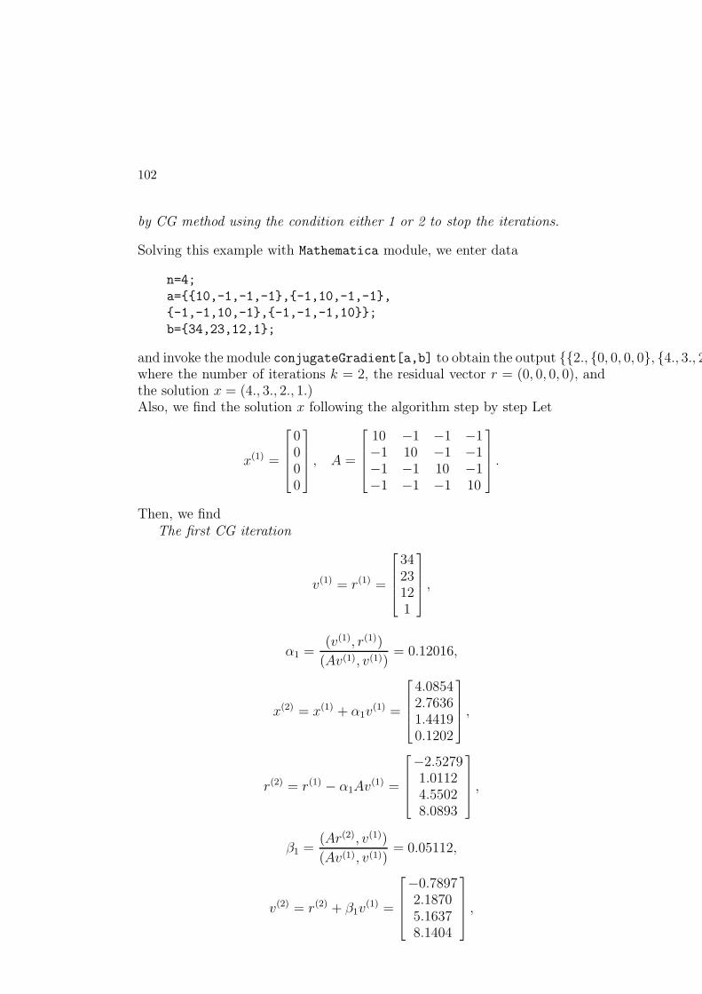
102

by CG method using the condition either 1 or 2 to stop the iterations.

Solving this example with Mathematica module, we enter data

n=4;

a={{10,-1,-1,-1},{-1,10,-1,-1},

{-1,-1,10,-1},{-1,-1,-1,10}};

b={34,23,12,1};

and invoke the module conjugateGradient[a,b] to obtain the output {{2., {0, 0, 0, 0}, {4., 3., 2where the number of iterations k = 2, the residual vector r = (0, 0, 0, 0), andthe solution x = (4., 3., 2., 1.)Also, we find the solution x following the algorithm step by step Let

x(1) =

0000

, A =

10 −1 −1 −1−1 10 −1 −1−1 −1 10 −1−1 −1 −1 10

.

Then, we findThe first CG iteration

v(1) = r(1) =

3423121

,

α1 =(v(1), r(1))

(Av(1), v(1))= 0.12016,

x(2) = x(1) + α1v(1) =

4.08542.76361.44190.1202

,

r(2) = r(1) − α1Av(1) =

−2.52791.01124.55028.0893

,

β1 =(Ar(2), v(1))

(Av(1), v(1))= 0.05112,

v(2) = r(2) + β1v(1) =

−0.78972.18705.16378.1404

,

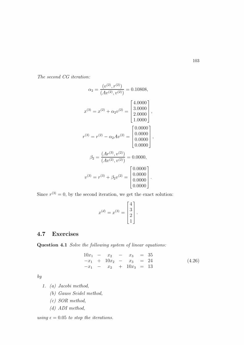
103

The second CG iteration:

α2 =(v(2), r(2))

(Av(2), v(2))= 0.10808,

x(3) = x(2) + α2v(2) =

4.00003.00002.00001.0000

,

r(3) = r(2) − α2Av(2) =

0.00000.00000.00000.0000

,

β2 =(Ar(3), v(2))

(Av(2), v(2))= 0.0000,

v(3) = r(3) + β2v(2) =

0.00000.00000.00000.0000

.

Since r(3) = 0, by the second iteration, we get the exact solution:

x(d) = x(3) =

4321

.

4.7 Exercises

Question 4.1 Solve the following system of linear equations:

10x1 − x2 − x3 = 35−x1 + 10x2 − x3 = 24−x1 − x2 + 10x3 = 13

(4.26)

by

1. (a) Jacobi method,

(b) Gauss Seidel method,

(c) SOR method,

(d) ADI method,

using ǫ = 0.05 to stop the iterations.

104

Question 4.2 Investigate the convergence of Jacobi and Gauss Seidel iterativemethods for the following system of linear equations:

2x1 − x2 − x3 = 3−x1 + 2x2 − x3 = 0−x1 − x2 + 2x3 = −3

Question 4.3 Solve the system of equations

3x1 − x2 − x3 = −1−x1 + 3x2 − x3 = 2−x1 − x2 + 3x3 = 6

by CG method.

Question 4.4 (a) State the necessary and sufficient conditions for conver-gence of the stationary linear one step iterative methods. Show that theiterative method

x(m+1) = G x(m) + F, m = 0, 1, 2, ...

satisfies the necessary and sufficient condition when

G =1

10

3 1

1 3

(b) State a sufficient condition for convergence of the Jacobi and Gauss Seideliterative methods. Show the the Jacobi and Gauss Seidel iterative methodsare convergent when they are applied to the system of equations

5x1 − 2x2 − x3 = 10

−2x1 + 10x2 − x3 = 13

−x1 − x2 + 5x3 = 0

(4.27)

(c) Solve the system of equations (4.27) by Jacobi and Gauss Seidel iterativemethods using starting vector x(0) = {2.5, 1.5, 1} with the accuracy ǫ =0.01

Question 4.5 (a) State the algorithm of the Conjugate Gradient Method forsolving a linear system of equations Ax = b where A = {aij}, i, j =1, 2, ..., n. is a symmetric non-singular matrix

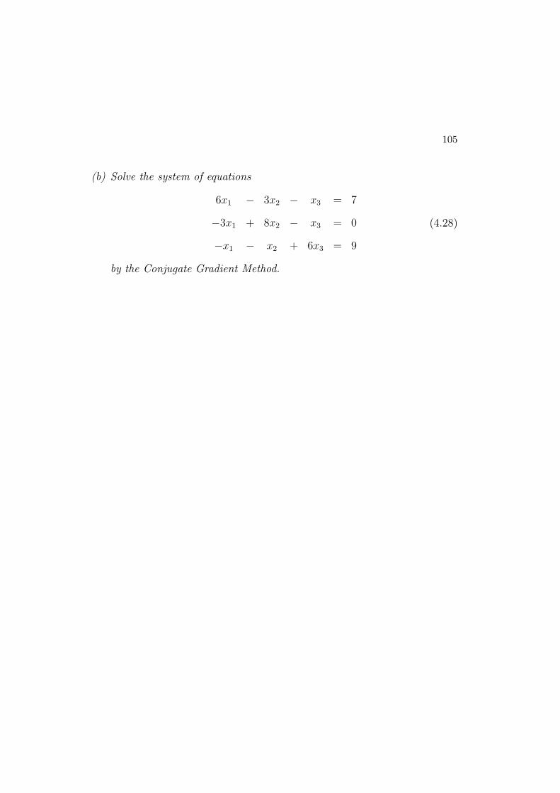
105

(b) Solve the system of equations

6x1 − 3x2 − x3 = 7

−3x1 + 8x2 − x3 = 0

−x1 − x2 + 6x3 = 9

(4.28)

by the Conjugate Gradient Method.

106

4.8 References

[1 ] Conte, S. D., & de Boor, C., (1983), Elementary Numerical Analysis,Algorithmic Approach, McGraw-Hill.

[5 ] Duff, I.S., Erisman, A.M., & Reid, J.K., (1986), Direct Methods forSparse Matrices, Clarendon Press-Oxford.

[6 ] Faddeev, D.K., & Faddeeva, W.N., (1963), Numerical Methods in LinearAlgebra, State Publisher, Ser.,Phys. & Maths.

[7 ] Golub, G., & Van Loan, C.F., (1983), Matrix Computations, John Hop-kins University Press.

[8 ] Hageman, L.A., & Young, D.M., (1981), Applied Iterative Methods,Academic Press.

[13 ] Moris, J.L., (1983), Computational Methods in Numerical Analysis,John Wiley & Sons.

[17 ] Ralston, A., (1965), A First Course in Numerical Analysis, McGraw-Hill.

[18 ] Stoer, J. & Bulrisch R. (1980), Introduction to Numerical Analysis,Springer-Verlag

[19 ] Varga, R.S. (1962), Matrix Iterative Analysis, Printice-Hall, INC.

[ 21 ] Wolfram, S., (1992), Mathematica a System for Doing Mathematics byComputers, Addison-Wesley Publishing Company.

[22 ] Young, D.M. (1971), Iterative Solution of Large Linear Systems, Aca-demic Press.