Embed Size (px)
Citation preview
Lecture Notes on
Compositional Data Analysis
Vera Pawlowsky-GlahnUniversity of Girona, Spain
Juan Jos EgozcueTechnical University of Catalonia, Spain
Raimon Tolosana-DelgadoTechnical University of Catalonia, Spain
March 2011

ii

i
Prof. Dr. Vera Pawlowsky-GlahnCatedratica de Universidad (full professor)University of GironaDept. of Computer Science and Applied MathematicsCampus Montilivi — P-4, E-17071 Girona, [email protected]
Prof. Dr. Juan Jose EgozcueCatedratico de Universidad (full professor)Technical University of CataloniaDept. of Applied Mathematics IIICampus Nord c/Jordi Girona 1-3, C-2, E-08034 Barcelona, [email protected]
Dr. Raimon Tolosana-DelgadoInvestigador Juan de la CiervaTechnical University of CataloniaMaritime Engineering Laboratory (LIM-UPC)Campus Nord c/Jordi Girona 1-3, D-1, E-08034 Barcelona, [email protected]
ii
Preface
These notes have been prepared as support to a short course on compositionaldata analysis. The first version dates back to the year 2000. Their aim is totransmit the basic concepts and skills for simple applications, thus setting thepremises for more advanced projects. The notes have been updated over theyears. But one should be aware that frequent updates will be still required inthe near future, as the theory presented here is a field of active research.
The notes are based both on the monograph by John Aitchison, Statis-tical analysis of compositional data (1986), and on recent developments thatcomplement the theory developed there, mainly those by Aitchison (1997); Bar-celo-Vidal et al. (2001); Billheimer et al. (2001); Pawlowsky-Glahn and Egozcue(2001, 2002); Aitchison et al. (2002); Egozcue et al. (2003); Pawlowsky-Glahn(2003) and Egozcue and Pawlowsky-Glahn (2005). To avoid constant referencesto mentioned documents, only complementary references will be given withinthe text.
Readers should take into account that for a thorough understanding of com-positional data analysis, a good knowledge in standard univariate statistics, ba-sic linear algebra and calculus, complemented with an introduction to appliedmultivariate statistical analysis, is a must. The specific subjects of interest inmultivariate statistics in real space can be learned in parallel from standardtextbooks, like for instance Krzanowski (1988) and Krzanowski and Marriott(1994) (in English), Fahrmeir and Hamerle (1984) (in German), or Pena (2002)(in Spanish). Thus, the intended audience goes from advanced students in ap-plied sciences to practitioners.
Concerning notation, it is important to note that, to conform to the standardpraxis of registering samples as a matrix where each row is a sample and eachcolumn is a variate, vectors will be considered as row vectors to make the transferfrom theoretical concepts to practical computations easier.
Most chapters end with a list of exercises. They are formulated in such away that they have to be solved using an appropriate software. CoDaPack is auser friendly freeware to facilitate this task and it can be downloaded from theweb. Details about this package can be found in Thio-Henestrosa and Martın-Fernandez (2005) or Thio-Henestrosa et al. (2005). Those interested in workingwith R (or S-plus) may use the full-fledged package “compositions” by vanden Boogaart and Tolosana-Delgado (2005).
Girona, Vera Pawlowsky-GlahnBarcelona, Juan Jose EgozcueMarch 2011 Raimon Tolosana-Delgado

iii
Acknowledgements. We acknowledge the many comments made by readers,pointing at small and at important errors in the text. They all have contributedto improve the Lecture Notes presented here. We appreciate also the supportreceived from our Universities, research groups, from the Spanish Ministry of Ed-ucation and Science under projects: ‘Ingenio Mathematica (i-MATH)’ Ref. No.CSD2006-00032 and ‘CODA-RSS’ Ref. MTM2009-13272; and from the Agenciade Gestio d’Ajuts Universitaris i de Recerca of the Generalitat de Catalunya un-der the project with Ref: 2009SGR424.

iv
Contents
1 Introduction 1
2 Compositional data and their sample space 52.1 Basic concepts . . . . . . . . . . . . . . . . . . . . . . . . . . . . 52.2 Principles of compositional analysis . . . . . . . . . . . . . . . . . 7
2.2.1 Scale invariance . . . . . . . . . . . . . . . . . . . . . . . . 72.2.2 Permutation invariance . . . . . . . . . . . . . . . . . . . 92.2.3 Subcompositional coherence . . . . . . . . . . . . . . . . . 10
2.3 Exercises . . . . . . . . . . . . . . . . . . . . . . . . . . . . . . . 10
3 The Aitchison geometry 133.1 General comments . . . . . . . . . . . . . . . . . . . . . . . . . . 133.2 Vector space structure . . . . . . . . . . . . . . . . . . . . . . . . 143.3 Inner product, norm and distance . . . . . . . . . . . . . . . . . . 163.4 Geometric figures . . . . . . . . . . . . . . . . . . . . . . . . . . . 173.5 Exercises . . . . . . . . . . . . . . . . . . . . . . . . . . . . . . . 18
4 Coordinate representation 214.1 Introduction . . . . . . . . . . . . . . . . . . . . . . . . . . . . . . 214.2 Compositional observations in real space . . . . . . . . . . . . . . 224.3 Generating systems . . . . . . . . . . . . . . . . . . . . . . . . . . 224.4 Orthonormal coordinates . . . . . . . . . . . . . . . . . . . . . . 244.5 Working in coordinates . . . . . . . . . . . . . . . . . . . . . . . . 284.6 Additive log-ratio coordinates . . . . . . . . . . . . . . . . . . . . 314.7 Simplicial matrix notation . . . . . . . . . . . . . . . . . . . . . . 324.8 Exercises . . . . . . . . . . . . . . . . . . . . . . . . . . . . . . . 34
5 Exploratory data analysis 375.1 General remarks . . . . . . . . . . . . . . . . . . . . . . . . . . . 375.2 Centre, total variance and variation matrix . . . . . . . . . . . . 385.3 Centring and scaling . . . . . . . . . . . . . . . . . . . . . . . . . 395.4 The biplot: a graphical display . . . . . . . . . . . . . . . . . . . 40
5.4.1 Construction of a biplot . . . . . . . . . . . . . . . . . . . 405.4.2 Interpretation of a compositional biplot . . . . . . . . . . 42
v
vi CONTENTS
5.5 Exploratory analysis of coordinates . . . . . . . . . . . . . . . . . 435.6 Illustration . . . . . . . . . . . . . . . . . . . . . . . . . . . . . . 445.7 Linear trend using principal components . . . . . . . . . . . . . . 505.8 Exercises . . . . . . . . . . . . . . . . . . . . . . . . . . . . . . . 52
6 Distributions on the simplex 556.1 The normal distribution on SD . . . . . . . . . . . . . . . . . . . 556.2 Other distributions . . . . . . . . . . . . . . . . . . . . . . . . . . 566.3 Tests of normality on SD . . . . . . . . . . . . . . . . . . . . . . 56
6.3.1 Marginal univariate distributions . . . . . . . . . . . . . . 576.3.2 Bivariate angle distribution . . . . . . . . . . . . . . . . . 596.3.3 Radius test . . . . . . . . . . . . . . . . . . . . . . . . . . 60
6.4 Exercises . . . . . . . . . . . . . . . . . . . . . . . . . . . . . . . 61
7 Statistical inference 637.1 Testing hypothesis about two groups . . . . . . . . . . . . . . . . 637.2 Probability and confidence regions for compositional data . . . . 667.3 Exercises . . . . . . . . . . . . . . . . . . . . . . . . . . . . . . . 67
8 Compositional processes 698.1 Linear processes: exponential growth or decay of mass . . . . . . 698.2 Complementary processes . . . . . . . . . . . . . . . . . . . . . . 728.3 Mixture process . . . . . . . . . . . . . . . . . . . . . . . . . . . . 76
9 Linear compositional models 799.1 Linear regression with compositional variables . . . . . . . . . . . 809.2 Regression with compositional covariates . . . . . . . . . . . . . . 839.3 Analysis of variance with compositional response . . . . . . . . . 849.4 Linear discrimination with compositional predictor . . . . . . . . 86
A Plotting a ternary diagram 91
B Parametrisation of an elliptic region 93
Chapter 1
Introduction
The awareness of problems related to the statistical analysis of compositionaldata analysis dates back to a paper by Karl Pearson (1897) which title begansignificantly with the words “On a form of spurious correlation ... ”. Sincethen, as stated in Aitchison and Egozcue (2005), the way to deal with this typeof data has gone through roughly four phases, which they describe as follows:
The pre-1960 phase rode on the crest of the developmental waveof standard multivariate statistical analysis, an appropriate form ofanalysis for the investigation of problems with real sample spaces.Despite the obvious fact that a compositional vector—with compo-nents the proportions of some whole—is subject to a constant-sumconstraint, and so is entirely different from the unconstrained vectorof standard unconstrained multivariate statistical analysis, scientistsand statisticians alike seemed almost to delight in applying all the in-tricacies of standard multivariate analysis, in particular correlationanalysis, to compositional vectors. We know that Karl Pearson,in his definitive 1897 paper on spurious correlations, had pointedout the pitfalls of interpretation of such activity, but it was notuntil around 1960 that specific condemnation of such an approachemerged.
In the second phase, the primary critic of the application of stan-dard multivariate analysis to compositional data was the geologistFelix Chayes (1960), whose main criticism was in the interpretationof product-moment correlation between components of a geochem-ical composition, with negative bias the distorting factor from theviewpoint of any sensible interpretation. For this problem of neg-ative bias, often referred to as the closure problem, Sarmanov andVistelius (1959) supplemented the Chayes criticism in geological ap-plications and Mosimann (1962) drew the attention of biologists toit. However, even conscious researchers, instead of working towardsan appropriate methodology, adopted what can only be described as
1
2 CHAPTER 1. INTRODUCTION
a pathological approach: distortion of standard multivariate tech-niques when applied to compositional data was the main goal ofstudy.
The third phase was the realisation by Aitchison in the 1980’sthat compositions provide information about relative, not absolute,values of components, that therefore every statement about a com-position can be stated in terms of ratios of components (Aitchison,1981, 1982, 1983, 1984). The facts that logratios are easier to handlemathematically than ratios and that a logratio transformation pro-vides a one-to-one mapping on to a real space led to the advocacyof a methodology based on a variety of logratio transformations.These transformations allowed the use of standard unconstrainedmultivariate statistics applied to transformed data, with inferencestranslatable back into compositional statements.
The fourth phase arises from the realisation that the internalsimplicial operation of perturbation, the external operation of pow-ering, and the simplicial metric, define a metric vector space (indeeda Hilbert space) (Billheimer et al., 1997, 2001; Pawlowsky-Glahnand Egozcue, 2001). So, many compositional problems can be inves-tigated within this space with its specific algebraic-geometric struc-ture. There has thus arisen a staying-in-the-simplex approach tothe solution of many compositional problems (Mateu-Figueras, 2003;Pawlowsky-Glahn, 2003). This staying-in-the-simplex point of viewproposes to represent compositions by their coordinates, as they livein an Euclidean space, and to interpret them and their relationshipsfrom their representation in the simplex. Accordingly, the samplespace of random compositions is identified to be the simplex witha simplicial metric and measure, different from the usual Euclideanmetric and Lebesgue measure in real space.
The third phase, which mainly deals with (log-ratio) transforma-tion of raw data, deserves special attention because these techniqueshave been very popular and successful over more than a century;from the Galton-McAlister introduction of such an idea in 1879 intheir logarithmic transformation for positive data, through variance-stabilising transformations for sound analysis of variance, to the gen-eral Box-Cox transformation (Box and Cox, 1964) and the impliedtransformations in generalised linear modeling. The logratio trans-formation principle was based on the fact that there is a one-to-one correspondence between compositional vectors and associatedlogratio vectors, so that any statement about compositions can bereformulated in terms of logratios, and vice versa. The advantage ofthe transformation is that it removes the problem of a constrainedsample space, the unit simplex, to one of an unconstrained space,multivariate real space, opening up all available standard multivari-ate techniques. The original transformations were principally theadditive logratio transformation (Aitchison, 1986, p.113) and the

3
centred logratio transformation (Aitchison, 1986, p.79). The logratiotransformation methodology seemed to be accepted by the statisticalcommunity; see for example the discussion of Aitchison (1982). Thelogratio methodology, however, drew fierce opposition from otherdisciplines, in particular from sections of the geological community.The reader who is interested in following the arguments that havearisen should examine the Letters to the Editor of MathematicalGeology over the period 1988 through 2002.
The notes presented here correspond to the fourth phase. They pretend tosummarise the state-of-the-art in the staying-in-the-simplex approach. There-fore, the first part will be devoted to the algebraic-geometric structure of thesimplex, which we call Aitchison geometry.

4 CHAPTER 1. INTRODUCTION
Chapter 2
Compositional data andtheir sample space
2.1 Basic concepts
Definition 2.1.1 A row vector, x = [x1, x2, . . . , xD], is defined as a D-partcomposition when all its components are strictly positive real numbers and theycarry only relative information.
Indeed, that compositional information is relative is implicitly stated in theunits, as they are usually parts of a whole, like weight or volume percent, ppm,ppb, or molar proportions. The most common examples have a constant sumκ and are known in the geological literature as closed data (Chayes, 1971).Frequently, κ = 1, which means that measurements have been made in, ortransformed to, parts per unit, or κ = 100, for measurements in percent. Otherunits are possible, like ppm or ppb, which are typical examples for composi-tional data where only a part of the composition has been recorded; or, asrecent studies have shown, even concentration units (mg/L, meq/L, molaritiesand molalities), where no constant sum can be feasibly defined (Buccianti andPawlowsky-Glahn, 2005; Otero et al., 2005).
Definition 2.1.2 The sample space of compositional data is the simplex, de-fined as
SD =
{x = [x1, x2, . . . , xD]
∣∣∣∣∣xi > 0, i = 1, 2, . . . , D;D∑
i=1
xi = κ
}. (2.1)
However, this definition does not include compositions in e.g. meq/L. There-fore, a more general definition, together with its interpretation, is given in Sec-tion 2.2.
The components of a vector in SD are called parts to remark their compo-sitional character.
5
6 CHAPTER 2. COMPOSITIONAL DATA AND THEIR SAMPLE SPACE
P
x1
x2
constant sum
P'
A
B
P
A B
C
p3
p1p2
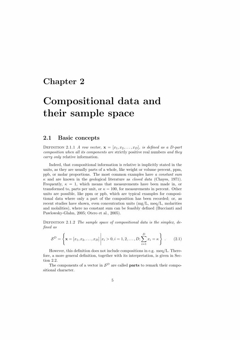
Figure 2.1: Left: Simplex imbedded in R3. Right: Ternary diagram.
Definition 2.1.3 For any vector of D real positive components
z = [z1, z2, . . . , zD] ∈ RD+
(zi > 0 for all i = 1, 2, . . . , D), the closure of z is defined as
C(z) =
[κ · z1∑D
i=1 zi
,κ · z2∑D
i=1 zi
, · · · ,κ · zD∑D
i=1 zi
].
The result is the same vector re-scaled so that the sum of its componentsis κ. This operation is required for a formal definition of subcomposition andfor inverse transformations. Note that κ depends on the units of measurement:usual values are 1 (proportions), 100 (%), 106 (ppm) and 109 (ppb).
Definition 2.1.4 Given a composition x, a subcomposition xs with s parts isobtained applying the closure operation to a subvector [xi1 , xi2 , . . . , xis ] of x.Subindexes i1, . . . , is tell which parts are selected in the subcomposition, notnecessarily the first s ones.
Very often, compositions contain many parts; e.g., the major oxide bulkcomposition of igneous rocks has around 10 elements, and they are but a fewof the total possible. Nevertheless, one seldom represents the full composi-tion. In fact, most of the applied literature on compositional data analysis(mainly in geology) restricts their figures to 3-part (sub)compositions. For 3parts, the simplex can be represented as an equilateral triangle (Figure 2.1left), with vertices at A = [κ, 0, 0], B = [0, κ, 0] and C = [0, 0, κ]. But thisis commonly visualised in the form of a ternary diagram—which is an equiva-lent representation—. A ternary diagram is an equilateral triangle such that ageneric sample p = [p1, p2, p3] will plot at a distance p1 from the opposite side ofvertex A, at a distance p2 from the opposite side of vertex B, and at a distancep3 from the opposite side of vertex C (Figure 2.1 right). The triplet [p1, p2, p3]is commonly called the barycentric coordinates of p, easily interpretable butuseless in plotting (plotting them would yield the three-dimensional left-hand
2.2. PRINCIPLES OF COMPOSITIONAL ANALYSIS 7
plot of Figure 2.1). What is needed to get the right-hand plot of Figure 2.1)is the expression of the coordinates of the vertices and of the samples in a 2-dimensional Cartesian coordinate system [u, v], and this is given in AppendixA.
Finally, if only some parts of the composition are available, a fill up orresidual value can be defined, or simply the observed subcomposition can beclosed. Note that, since one seldom analyses every possible part, in practice onlysubcompositions are analysed. In any case, both methods (fill-up or closure)should lead to identical, or at least compatible, results.
2.2 Principles of compositional analysis
Three conditions should be fulfilled by any statistical method to be applied tocompositions: scale invariance, permutation invariance, and subcompositionalcoherence (Aitchison, 1986).
2.2.1 Scale invariance
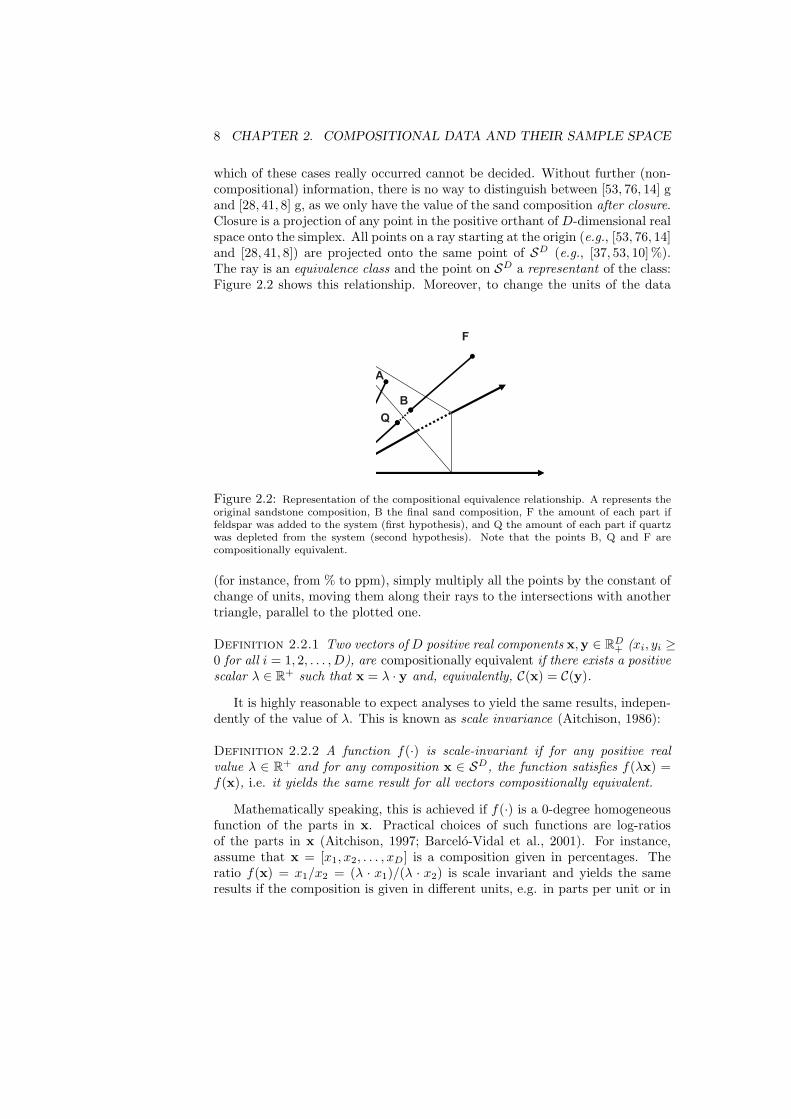
The most important characteristic of compositional data is that they carry onlyrelative information. Let us explain this concept with an example. In a paperwith the suggestive title of “unexpected trend in the compositional maturity ofsecond-cycle sands”, Solano-Acosta and Dutta (2005) the lithologic compositionof a sandstone and of its derived recent sands is analysed looking at the per-centage of grains made up of only quartz, of only feldspar, or of rock fragments.For medium sized grains coming from the parent sandstone, they report an av-erage composition [Q, F, R] = [53, 41, 6]%, whereas for the daughter sands themean values are [37, 53, 10]%. One expects that feldspar and rock fragmentsdecrease as the sediment matures, thus they should be less important in a sec-ond generation sand. “Unexpectedly” (or apparently), this does not happen intheir example. To pass from the parent sandstone to the daughter sand, sev-eral different changes are possible, yielding exactly the same final composition.Assume those values were weight percent (in g/100 g of bulk sediment). Then,one of the following might have happened:
• Q suffered no change passing from sandstone to sand, but per 100 g parentsandstone 35 g F and 8 g R were added to the sand (for instance, due tocomminution of coarser grains of F and R from the sandstone),
• F was unchanged, but per 100 g parent sandstone 25 g Q were depletedand at the same time 2 g R were added (for instance, because Q was bettercemented in the sandstone, thus it tends to form coarser grains),
• any combination of the former two extremes.
The first two cases yield, per 100 g parent sandstone, final masses of [53, 76, 14]g, respectively [28, 41, 8] g. In a purely compositional data set, we do not knowwhether mass was added or subtracted from the sandstone to the sand. Thus,
8 CHAPTER 2. COMPOSITIONAL DATA AND THEIR SAMPLE SPACE
which of these cases really occurred cannot be decided. Without further (non-compositional) information, there is no way to distinguish between [53, 76, 14] gand [28, 41, 8] g, as we only have the value of the sand composition after closure.Closure is a projection of any point in the positive orthant of D-dimensional realspace onto the simplex. All points on a ray starting at the origin (e.g., [53, 76, 14]and [28, 41, 8]) are projected onto the same point of SD (e.g., [37, 53, 10]%).The ray is an equivalence class and the point on SD a representant of the class:Figure 2.2 shows this relationship. Moreover, to change the units of the data
A
Q
B
F
Figure 2.2: Representation of the compositional equivalence relationship. A represents theoriginal sandstone composition, B the final sand composition, F the amount of each part iffeldspar was added to the system (first hypothesis), and Q the amount of each part if quartzwas depleted from the system (second hypothesis). Note that the points B, Q and F arecompositionally equivalent.
(for instance, from % to ppm), simply multiply all the points by the constant ofchange of units, moving them along their rays to the intersections with anothertriangle, parallel to the plotted one.
Definition 2.2.1 Two vectors of D positive real components x,y ∈ RD+ (xi, yi ≥
0 for all i = 1, 2, . . . , D), are compositionally equivalent if there exists a positivescalar λ ∈ R+ such that x = λ · y and, equivalently, C(x) = C(y).
It is highly reasonable to expect analyses to yield the same results, indepen-dently of the value of λ. This is known as scale invariance (Aitchison, 1986):
Definition 2.2.2 A function f(·) is scale-invariant if for any positive realvalue λ ∈ R+ and for any composition x ∈ SD, the function satisfies f(λx) =f(x), i.e. it yields the same result for all vectors compositionally equivalent.
Mathematically speaking, this is achieved if f(·) is a 0-degree homogeneousfunction of the parts in x. Practical choices of such functions are log-ratiosof the parts in x (Aitchison, 1997; Barcelo-Vidal et al., 2001). For instance,assume that x = [x1, x2, . . . , xD] is a composition given in percentages. Theratio f(x) = x1/x2 = (λ · x1)/(λ · x2) is scale invariant and yields the sameresults if the composition is given in different units, e.g. in parts per unit or in
2.2. PRINCIPLES OF COMPOSITIONAL ANALYSIS 9
parts per million, because units cancel in the ratio. However, ratios depend onthe ordering of parts because x1/x2 6= x2/x1. A convenient transformation ofratios is the corresponding log-ratio, f(x) = ln(x1/x2). Now, the inversion ofthe ratio only produces a change of sign, thus giving a symmetry to f(·) withrespect to the ordering of parts.
More complicated log-ratios are useful. For instance, define
f(x) = lnxα1
1 · xα22 · · ·xαs
s
x−αs+1s+1 · x−αs+2
s+2 · · ·x−αD
D
=D∑
i=1
αi ln xi ,
where powers αi are real constants (positive or negative). In the ratio expression,for i = s + 1, s + 2, . . . , D, αi are assumed negative, thus appearing in thedenominator with a positive value −αi. For this log-ratio to be scale invariant,the sum of all powers should be null. Scale invariant log-ratios are called log-contrasts (Aitchison, 1986).
Definition 2.2.3 Consider a composition x = [x1, x2, . . . , xD]. A log-contrastis a function
f(x) =D∑
i=1
αi ln xi , withD∑
i=1
αi = 0 .
In applications, some log-contrasts may be easily interpreted. A typical exampleis chemical equilibrium. Consider a chemical D-part composition, denoted xexpressed in ppm of mass. A chemical reaction involving four species may be
α1x1 + α2x2 α3x3 + α4x4 ,
where other parts are not involved. The αi’s, called stoichiometric coefficients,are normally known. If the reaction is mass preserving, then α1 +α2 = α3 +α4.Whenever this chemical reaction is in equilibrium, the log-contrast
lnxα1
1 · xα22
xα33 · xα4
4
should be constant and, therefore, it is readily interpreted.
2.2.2 Permutation invariance
A function is permutation-invariant if it yields equivalent results when the or-dering of the parts in the composition is changed. Two examples might illustratewhat “equivalent” means here. The distance between the initial sandstone andthe final sand compositions should be the same working with [Q,F, R] or work-ing with [F, R,Q] (or any other permutation of the parts). On the other side,if interest lies in the change occurred from sandstone to sand, results should beequal after reordering. A classical way to get rid of the singularity of the clas-sical covariance matrix of compositional data is to erase one component: this
10 CHAPTER 2. COMPOSITIONAL DATA AND THEIR SAMPLE SPACE
procedure is not permutation-invariant, as results will largely depend on whichcomponent is erased.
However, ordered compositional data are frequent. A typical case corre-sponds to the discretisation of a continuous variable. Some interval categoriesare defined on the span of the variable, and then the number of occurrencesin each category are recorded as frequencies. These frequencies can be consid-ered as a composition although categories are still ordered. The informationconcerning the ordering will be lost in a standard compositional analysis.
2.2.3 Subcompositional coherence
The final condition is subcompositional coherence: subcompositions should be-have like orthogonal projections in conventional real analysis. The size of aprojected segment is less than or equal to the size of the segment itself. Thisgeneral principle, though shortly stated, has several practical implications, ex-plained in the next chapters. The most illustrative, however, are the following.
• The distance measured between two full compositions must be greaterthan (or at least equal to) the distance between them when consideringany subcomposition. This particular behaviour of the distance is calledsubcompositional dominance. Exercise 2.3.4 proves that the Euclideandistance between compositional vectors does not fulfill this condition, andit is thus ill-suited to measure distance between compositions.
• If a non-informative part is erased, results should not change; for instanceif hydrogeochemical data are available, and interest lies in classifying thekind of rocks washed by the water, in general the relations between somemajor oxides and ions will be used (SO2+
4 , HCO−3 , Cl−, to mention afew), and the same results should be obtained taking meq/L (includingimplicitly water content), or weight percent of the ions of interest.
Subcompositional coherence can be summarized as: (a) distances betweentwo compositions should decrease when subcompositions of the original onesare considered; (b) scale invariance is preserved within arbitrary subcomposi-tions (Egozcue, 2009). This means that the ratios between any parts in thesubcomposition should be equal to the ratios in the original composition.
2.3 Exercises
Exercise 2.3.1 If data are measured in ppm, what is the value of the constantκ in definition (2.1.2)?
Exercise 2.3.2 Plot a ternary diagram using different values for the constantsum κ.
Exercise 2.3.3 Verify that data in table 2.1 satisfy the conditions for beingcompositional. Plot them in a ternary diagram.
2.3. EXERCISES 11
Table 2.1: Simulated data set (3 parts, 20 samples).
1 2 3 4 5 6 7 8 9 10x1 79.07 31.74 18.61 49.51 29.22 21.99 11.74 24.47 5.14 15.54x2 12.83 56.69 72.05 15.11 52.36 59.91 65.04 52.53 38.39 57.34x3 8.10 11.57 9.34 35.38 18.42 18.10 23.22 23.00 56.47 27.11
11 12 13 14 15 16 17 18 19 20x1 57.17 52.25 77.40 10.54 46.14 16.29 32.27 40.73 49.29 61.49x2 3.81 23.73 9.13 20.34 15.97 69.18 36.20 47.41 42.74 7.63x3 39.02 24.02 13.47 69.12 37.89 14.53 31.53 11.86 7.97 30.88
Exercise 2.3.4 Compute the Euclidean distance between the first two vectorsof table 2.1. Imagine originally a fourth variable x4 was measured, constant forall samples and equal to 5%. Take the first two vectors, close them to sum up to95%, add the fourth variable to them (so that they sum up to 100%) and computethe Euclidean distance between the closed vectors. If the Euclidean distance issubcompositionally dominant, the distance measured in 4 parts must be greateror equal to the distance measured in the 3 part subcomposition.

12 CHAPTER 2. COMPOSITIONAL DATA AND THEIR SAMPLE SPACE
Chapter 3
The Aitchison geometry
3.1 General comments
In real space we are used to add vectors, to multiply them by a constant orscalar value, to look for properties like orthogonality, or to compute the distancebetween two points. All this, and much more, is possible because the real spaceis a linear vector space with an Euclidean metric structure. We are familiarwith its geometric structure, the Euclidean geometry, and we represent ourobservations within this geometry. But this geometry is not a proper geometryfor compositional data.
To illustrate this assertion, consider the compositions
[5, 65, 30], [10, 60, 30], [50, 20, 30], and [55, 15, 30].
Intuitively we would say that the difference between [5, 65, 30] and [10, 60, 30]is not the same as the difference between [50, 20, 30] and [55, 15, 30]. The Eu-clidean distance between them is certainly the same, as there is a difference of5 units both between the first and the second components, but in the first casethe proportion in the first component is doubled, while in the second case therelative increase is about 10%, and this relative difference seems more adequateto describe compositional variability.
This is not the only reason for discarding Euclidean geometry as a proper toolfor analysing compositional data. Problems might appear in many situations,like those where results end up outside the sample space, e.g. when translatingcompositional vectors, or computing joint confidence regions for random compo-sitions under assumptions of normality, or using hexagonal confidence regions.This last case is paradigmatic, as such hexagons are often naively cut whenthey lay partly outside the ternary diagram, and this without regard to anyprobability adjustment. This kind of problems are not just theoretical: they arepractical and interpretative.
What is needed is a sensible geometry to work with compositional data. Inthe simplex, things appear not as simple as they (apparently) are in real space,
13
14 CHAPTER 3. THE AITCHISON GEOMETRY
but it is possible to find a way of working in it that is completely analogous.In fact, it is possible to define two operations which give the simplex a vectorspace structure. The first one is perturbation, which is analogous to additionin real space, the second one is powering, which is analogous to multiplicationby a scalar in real space. Both require in their definition the closure operation;recall that closure is nothing else but the projection of a vector with positivecomponents onto the simplex. Moreover, it is possible to obtain a Euclideanvector space structure on the simplex, just adding an inner product, a norm anda distance to the previous definitions. With the inner product compositions canbe projected onto particular directions, one can check for orthogonality anddetermine angles between compositional vectors; with the norm the length ofa composition can be computed; the possibilities of a distance should be clear.With all together one can operate in the simplex in the same way as one operatesin real space.
3.2 Vector space structure
The basic operations required for a vector space structure of the simplex follow.They use the closure operation given in Definition 2.1.3.
Definition 3.2.1 Perturbation of a composition x ∈ SD by a composition y ∈SD,
x⊕ y = C [x1y1, x2y2, . . . , xDyD] .
Definition 3.2.2 Power transformation or powering of a composition x ∈ SD
by a constant α ∈ R,α¯ x = C [xα
1 , xα2 , . . . , xα
D] .
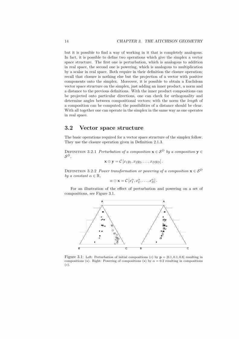
For an illustration of the effect of perturbation and powering on a set ofcompositions, see Figure 3.1.
Figure 3.1: Left: Perturbation of initial compositions (◦) by p = [0.1, 0.1, 0.8] resulting incompositions (?). Right: Powering of compositions (?) by α = 0.2 resulting in compositions(◦).
3.2. VECTOR SPACE STRUCTURE 15
The simplex , (SD,⊕,¯), with perturbation and powering, is a vector space.This means the following properties hold, making them analogous to translationand scalar multiplication:
Property 3.2.1 (SD,⊕) has a commutative group structure; i.e., for x, y,z ∈ SD it holds
1. commutative property: x⊕ y = y ⊕ x;
2. associative property: (x⊕ y)⊕ z = x⊕ (y ⊕ z);
3. neutral element:
n = C [1, 1, . . . , 1] =[
1D
,1D
, . . . ,1D
];
n is the barycentre of the simplex and is unique;
4. inverse of x: x−1 = C [x−1
1 , x−12 , . . . , x−1
D
]; thus, x⊕x−1 = n. By analogy
with standard operations in real space, we will write x⊕ y−1 = xª y.
Property 3.2.2 Powering satisfies the properties of an external product. Forx,y ∈ SD, α, β ∈ Rit holds
1. associative property: α¯ (β ¯ x) = α · β)¯ x;
2. distributive property 1: α¯ (x⊕ y) = (α¯ x)⊕ (α¯ y);
3. distributive property 2: (α + β)¯ x = (α¯ x)⊕ (β ¯ x);
4. neutral element: 1¯ x = x; the neutral element is unique.
Note that the closure operation cancels out any constant and, thus, theclosure constant itself is not important from a mathematical point of view.This fact allows us to omit the closure in intermediate steps of any computationwithout problem. It has also important implications for practical reasons, asshall be seen during simplicial principal component analysis. We can expressthis property for z ∈ RD
+ and x ∈ SD as
x⊕ (α¯ z) = x⊕ (α¯ C(z)). (3.1)
Nevertheless, one should be always aware that the closure constant is veryimportant for the correct interpretation of the units of the problem at hand.Therefore, controlling for the right units should be the last step in any analysis.
16 CHAPTER 3. THE AITCHISON GEOMETRY
3.3 Inner product, norm and distance
To obtain a Euclidean vector space structure, we take the following inner prod-uct, with associated norm and distance:
Definition 3.3.1 Inner product of x,y ∈ SD,
〈x,y〉a =1
2D
D∑
i=1
D∑
j=1
lnxi
xjln
yi
yj.
Definition 3.3.2 Norm of x ∈ SD,
‖x‖a =
√√√√ 12D
D∑
i=1
D∑
j=1
(ln
xi
xj
)2
.
Definition 3.3.3 Distance between x and y ∈ SD,
da(x,y) = ‖xª x‖a =
√√√√ 12D
D∑
i=1
D∑
j=1
(ln
xi
xj− ln
yi
yj
)2
.
In practice, alternative but equivalent expressions of the inner product, normand distance may be useful. Three possible alternatives for the inner productfollow:
〈x,y〉a =1D
D−1∑
i=1
D∑
j=i+1
lnxi
xjln
yi
yj
=D∑
i=1
ln xi ln yi − 1D
D∑
j=1
ln xj
(D∑
k=1
ln yk
)
=D∑
i=1
lnxi
g(x)· ln yi
g(y).
where g(·) denotes the geometric mean of the arguments. The last expressionin 3.2 corresponds to an ordinary inner product of two real vectors. These vec-tors are called centered log-ratio (clr) of x, y, as defined in Chapter 4. Notethat notation
∑i<j means exactly
∑D−1i=1
∑Dj=i+1. Moreover, in the previous
expressions, simple logratios, ln(xi/xj), are null whenever i = j; in these cir-cumstances,
∑D−1i=1
∑Dj=i+1 = (1/2)
∑Di=1
∑Dj=1.
To refer to the properties of (SD,⊕,¯) as an Euclidean linear vector space,we shall talk globally about the Aitchison geometry on the simplex, and inparticular about the Aitchison distance, norm and inner product. Note that inmathematical textbooks, such a linear vector space is called either real Euclideanspace or finite dimensional real Hilbert space.
3.4. GEOMETRIC FIGURES 17
The algebraic-geometric structure of SD satisfies standard properties, likecompatibility of the distance with perturbation and powering, i.e.
da(p⊕ x,p⊕ y) = da(x,y), da(α¯ x, α¯ y) = |α|da(x,y) ,
for any x,y,p ∈ SD and α ∈ R. Other typical properties of metric spaces arevalid for SD. Some of them follow:
1. Cauchy-Schwartz inequality:
|〈x,y〉a| ≤ ‖x‖a · ‖y‖a ;
2. Pythagoras: If x, y are orthogonal, i.e. 〈x,y〉a = 0, then
‖xª y‖2a = ‖x‖2a + ‖y‖2a ;
3. Triangular inequality:
da(x,y) ≤ da(x, z) + da(y, z) .
For a discussion of these and other properties, see Billheimer et al. (2001) orPawlowsky-Glahn and Egozcue (2001). For a comparison with other measuresof difference obtained as restrictions of distances in RD to SD, see Martın-Fernandez et al. (1998, 1999); Aitchison et al. (2000) or Martın-Fernandez(2001). The Aitchison distance is subcompositionally coherent, as all this setof operations induce the same linear vector space structure in the subspace cor-responding to the subcomposition. Finally, the distance is subcompositionallydominant (Exercise 3.5.7).
3.4 Geometric figures
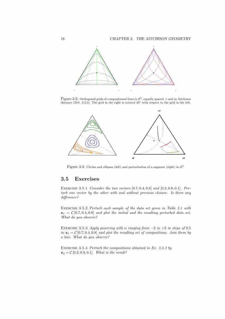
Within this framework, we can define lines in SD, which we call compositionallines, as y = x0 ⊕ (α¯ x), with x0 the starting point and x the leading vector.Note that y, x0 and x are elements of SD, while the coefficient α varies inR. To illustrate what we understand by compositional lines, Figure 3.2 showstwo families of parallel lines in a ternary diagram, forming a square, orthogonalgrid of side equal to one Aitchison distance unit. Recall that parallel lineshave the same leading vector, but different starting points, like for instancey1 = x1 ⊕ (α ¯ x) and y2 = x2 ⊕ (α ¯ x), while orthogonal lines are those forwhich the inner product of the leading vectors is zero, i.e., for y1 = x0⊕(α1¯x1)and y2 = x0 ⊕ (α2 ¯ x2), with x0 their intersection point and x1, x2 thecorresponding leading vectors, it holds 〈x1,x2〉a = 0. Thus, orthogonal meanshere that the inner product given in Definition 3.3.1 of the leading vectors of twolines, one of each family, is zero, and one Aitchison distance unit is measuredby the distance given in Definition 3.3.3.
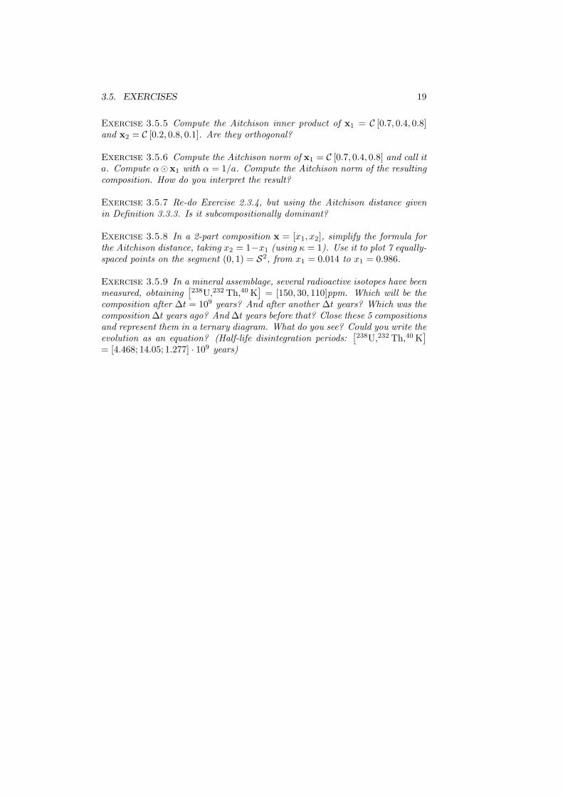
Once we have a well defined geometry, it is straightforward to define anygeometric figure, like for instance circles, ellipses, or rhomboids, as illustratedin Figure 3.3.
18 CHAPTER 3. THE AITCHISON GEOMETRY
x y
z
x y
z
Figure 3.2: Orthogonal grids of compositional lines in S3, equally spaced, 1 unit in Aitchisondistance (Def. 3.3.3). The grid in the right is rotated 45o with respect to the grid in the left.
x2
x1
x3
n
Figure 3.3: Circles and ellipses (left) and perturbation of a segment (right) in S3.
3.5 Exercises
Exercise 3.5.1 Consider the two vectors [0.7, 0.4, 0.8] and [0.2, 0.8, 0.1]. Per-turb one vector by the other with and without previous closure. Is there anydifference?
Exercise 3.5.2 Perturb each sample of the data set given in Table 2.1 withx1 = C [0.7, 0.4, 0.8] and plot the initial and the resulting perturbed data set.What do you observe?
Exercise 3.5.3 Apply powering with α ranging from −3 to +3 in steps of 0.5to x1 = C [0.7, 0.4, 0.8] and plot the resulting set of compositions. Join them bya line. What do you observe?
Exercise 3.5.4 Perturb the compositions obtained in Ex. 3.5.3 byx2 = C [0.2, 0.8, 0.1]. What is the result?
3.5. EXERCISES 19
Exercise 3.5.5 Compute the Aitchison inner product of x1 = C [0.7, 0.4, 0.8]and x2 = C [0.2, 0.8, 0.1]. Are they orthogonal?
Exercise 3.5.6 Compute the Aitchison norm of x1 = C [0.7, 0.4, 0.8] and call ita. Compute α¯x1 with α = 1/a. Compute the Aitchison norm of the resultingcomposition. How do you interpret the result?
Exercise 3.5.7 Re-do Exercise 2.3.4, but using the Aitchison distance givenin Definition 3.3.3. Is it subcompositionally dominant?
Exercise 3.5.8 In a 2-part composition x = [x1, x2], simplify the formula forthe Aitchison distance, taking x2 = 1−x1 (using κ = 1). Use it to plot 7 equally-spaced points on the segment (0, 1) = S2, from x1 = 0.014 to x1 = 0.986.
Exercise 3.5.9 In a mineral assemblage, several radioactive isotopes have beenmeasured, obtaining
[238U,232 Th,40 K
]= [150, 30, 110]ppm. Which will be the
composition after ∆t = 109 years? And after another ∆t years? Which was thecomposition ∆t years ago? And ∆t years before that? Close these 5 compositionsand represent them in a ternary diagram. What do you see? Could you write theevolution as an equation? (Half-life disintegration periods:
[238U,232 Th,40 K
]= [4.468; 14.05; 1.277] · 109 years)

20 CHAPTER 3. THE AITCHISON GEOMETRY
Chapter 4
Coordinate representation
4.1 Introduction
J. Aitchison (1986) used the fact that for compositional data size is irrelevant—as interest lies in relative proportions of the components measured—to introducetransformations based on ratios, the essential ones being the additive log-ratiotransformation (alr) and the centred log-ratio transformation (clr). Then, heapplied classical statistical analysis to the transformed observations, using thealr transformation for modeling, and the clr transformation for those techniquesbased on a metric. The underlying reason was, that the alr transformation doesnot preserve distances, whereas the clr transformation preserves distances butleads to a singular covariance matrix. In mathematical terms, we say thatthe alr transformation is an isomorphism, but not an isometry, while the clrtransformation is an isometry, and thus also an isomorphism, but between SD
and a subspace of RD, leading to degenerate distributions. Thus, Aitchison’sapproach opened up a rigorous strategy, but care had to be applied when usingeither of both transformations.
Using the Euclidean vector space structure, it is possible to give an algebraic-geometric foundation to his approach, and it is possible to go even a step further.Within this framework, a transformation of coefficients is equivalent to expressobservations in a different coordinate system. We are used to work in an orthog-onal system, known as a Cartesian coordinate system; we know how to changecoordinates within this system and how to rotate axis. But neither the clr northe alr transformations can be directly associated with an orthogonal coordi-nate system in the simplex, a fact that lead Egozcue et al. (2003) to define anew transformation, called ilr (for isometric logratio) transformation, which isan isometry between SD and RD−1, thus avoiding the drawbacks of both thealr and the clr. The ilr stands actually for the association of coordinates withcompositions in an orthonormal system in general, and this is the framework weare going to present here, together with a particular kind of coordinates, namedbalances, because of their usefulness for modeling and interpretation.
21
22 CHAPTER 4. COORDINATE REPRESENTATION
4.2 Compositional observations in real space
Compositions in SD are usually expressed in terms of the canonical basis{~e1,~e2, . . . ,~eD} of RD. In fact, any vector x ∈ RD can be written as
x = x1 [1, 0, . . . , 0] + x2 [0, 1, . . . , 0] + · · ·+ xD [0, 0, . . . , 1] =D∑
i=1
xi · ~ei , (4.1)
and this is the way we are used to interpret it. The problem is, that the set ofvectors {~e1,~e2, . . . ,~eD} is neither a generating system nor a basis with respectto the vector space structure of SD defined in Chapter 3. In fact, not everycombination of coefficients gives an element of SD (negative and zero values arenot allowed), and the ~ei do not belong to the simplex as defined in Equation(2.1). Nevertheless, in many cases it is interesting to express results in termsof compositions (4.1), so that interpretations are feasible in usual units, andtherefore one of our purposes is to find a way to state statistically rigorousresults in this coordinate system.
4.3 Generating systems
A first step for defining an appropriate orthonormal basis consists in findinga generating system which can be used to build the basis. A natural way toobtain such a generating system is to take {w1,w2, . . . ,wD}, with
wi = C (exp(~ei)) = C [1, 1, . . . , e, . . . , 1] , i = 1, 2, . . . , D , (4.2)
where in each wi the number e is placed in the i-th column, and the operationexp(·) is assumed to operate component-wise on a vector. In fact, taking intoaccount Equation (3.1) and the usual rules of precedence for operations in avector space, i.e., first the external operation, ¯, and afterwards the internaloperation, ⊕, any vector x ∈ SD can be written
x =D⊕
i=1
ln xi ¯wi =
= ln x1 ¯ [e, 1, . . . , 1]⊕ ln x2 ¯ [1, e, . . . , 1]⊕ · · · ⊕ ln xD ¯ [1, 1, . . . , e] .
It is known that the coefficients with respect to a generating system are notunique; thus, the following equivalent expression can be used as well,
x =D⊕
i=1
lnxi
g(x)¯wi =
= lnx1
g(x)¯ [e, 1, . . . , 1]⊕ · · · ⊕ ln
xD
g(x)¯ [1, 1, . . . , e] ,
where
g(x) =
(D∏
i=1
xi
)1/D
= exp
(1D
D∑
i=1
ln xi
),
4.3. GENERATING SYSTEMS 23
is the component-wise geometric mean of the composition. One recognises in thecoefficients of this second expression the centred logratio transformation definedby Aitchison (1986). Note that one could indeed replace the denominator by anyconstant. This non-uniqueness is consistent with the concept of compositionsas equivalence classes (Barcelo-Vidal et al., 2001).
We will denote by clr the transformation that gives the expression of acomposition in centred logratio coefficients
clr(x) =[ln
x1
g(x), ln
x2
g(x), . . . , ln
xD
g(x)
]= ξ. (4.3)
The inverse transformation, which gives us the coefficients in the canonical basisof real space, is then
clr−1(ξ) = C [exp(ξ1), exp(ξ2), . . . , exp(ξD)] = x. (4.4)
The centred logratio transformation is symmetrical in the components, but theprice is a new constraint on the transformed sample: the sum of the compo-nents has to be zero. This means that the transformed sample will lie on aplane, which goes through the origin of RD and is orthogonal to the vector ofunities [1, 1, . . . , 1]. But, more importantly, it means also that for random com-positions the covariance matrix of ξ is singular, i.e. the determinant is zero.Certainly, generalised inverses can be used in this context when necessary, butnot all statistical packages are designed for it and problems might arise duringcomputation. Furthermore, clr coefficients are not subcompositionally coher-ent, because the geometric mean of the parts of a subcomposition g(xs) is notnecessarily equal to that of the full composition, and thus the clr coefficientsare in general not the same. A formal definition of the clr coefficients follows.
Definition 4.3.1 For a composition x ∈ SD, the clr coefficients are the com-ponents of ξ = [ξ1, ξ2, . . . , ξD] = clr(x), the unique vector satisfying
x = clr−1(ξ) = C (exp(ξ)) ,
D∑
i=1
ξi = 0 .
The i-th clr coefficient is
ξi = lnxi
g(x),
being g(x) the geometric mean of the components of x.
Although the clr coefficients are not coordinates with respect to a basis ofthe simplex, they have very important properties. Among them the translationof operations and metrics from the simplex into the real space deserves specialattention. Denote ordinary distance, norm and inner product in RD−1 by d(·, ·),‖ · ‖, and 〈·, ·〉 respectively. The following property holds.
24 CHAPTER 4. COORDINATE REPRESENTATION
Property 4.3.1 Consider xk ∈ SD and real constants α, β; then
clr(α¯ x1 ⊕ β ¯ x2) = α · clr(x1) + β · clr(x2) ;
〈x1,x2〉a = 〈clr(x1), clr(x2)〉 ; (4.5)
‖x1‖a = ‖clr(x1)‖ , da(x1,x2) = d(clr(x1), clr(x2)) .
4.4 Orthonormal coordinates
Omitting one vector of the generating system given in Equation (4.2) a basis isobtained. For example, omitting wD results in {w1,w2, . . . ,wD−1}. This basisis not orthonormal, as can be shown computing the inner product of any two ofits vectors. But a new basis, orthonormal with respect to the inner product, canbe readily obtained using the well-known Gram-Schmidt procedure (Egozcueet al., 2003). The basis thus obtained will be just one out of the infinitely manyorthonormal basis which can be defined in any Euclidean space. Therefore, itis convenient to study their general characteristics.
Let {e1, e2, . . . , eD−1} be a generic orthonormal basis of the simplex SD andconsider the (D−1, D)-matrix Ψ whose rows are clr(ei). An orthonormal basissatisfies that 〈ei, ej〉a = δij (δij is the Kronecker-delta, which is null for i 6= j,and one whenever i = j). This can be expressed using (4.5),
〈ei, ej〉a = 〈clr(ei), clr(ej)〉 = δij .
It implies that the (D − 1, D)-matrix Ψ satisfies ΨΨ′ = ID−1, being ID−1
the identity matrix of dimension D − 1. When the product of these matricesis reversed, then Ψ′Ψ = ID − (1/D)1′D1D, with ID the identity matrix ofdimension D, and 1D a D-row-vector of ones; note this is a matrix of rankD − 1. The compositions of the basis are recovered from Ψ using clr−1 in eachrow of the matrix. Recall that these rows of Ψ also add up to 0 because theyare clr coefficients (see Definition 4.3.1).
Once an orthonormal basis has been chosen, a composition x ∈ SD is ex-pressed as
x =D−1⊕
i=1
x∗i ¯ ei , x∗i = 〈x, ei〉a , (4.6)
where x∗ =[x∗1, x
∗2, . . . , x
∗D−1
]is the vector of coordinates of x with respect to
the selected basis. The function ilr : SD → RD−1, assigning the coordinates x∗
to x has been called ilr (isometric log-ratio) transformation, as it is an isometricisomorphism of vector spaces. For simplicity, sometimes this function is alsodenoted by h, i.e. ilr ≡ h and also the asterisk (∗) is used to denote coordinatesif convenient. The following properties hold.
Property 4.4.1 Consider xk ∈ SD and real constants α, β; then
h(α¯ x1 ⊕ β ¯ x2) = α · h(x1) + β · h(x2) = α · x∗1 + β · x∗2 ;
4.4. ORTHONORMAL COORDINATES 25
〈x1,x2〉a = 〈h(x1), h(x2)〉 = 〈x∗1,x∗2〉 ;
‖x1‖a = ‖h(x1)‖ = ‖x∗1‖ , da(x1,x2) = d(h(x1), h(x2)) = d(x∗1,x∗2) .
The main difference between Property 4.3.1 for clr and Property 4.4.1 for ilr isthat the former refers to vectors of coefficients in RD, whereas the latter dealswith vectors of coordinates in RD−1, thus matching the actual dimension of SD.
Taking into account Properties 4.3.1 and 4.4.1, and using the clr imagematrix of the basis, Ψ, the coordinates of a composition x can be expressed ina compact way. As written in (4.6), a coordinate is an Aitchison inner product,and it can be expressed as an ordinary inner product of the clr coefficients.Grouping all coordinates in a vector
x∗ = ilr(x) = h(x) = clr(x) ·Ψ′ , (4.7)
a simple matrix product is obtained.Inversion of ilr, i.e. recovering the composition from its coordinates, corre-
sponds to Equation (4.6). In fact, taking clr coefficients in both sides of (4.6)and taking into account Property 4.3.1,
clr(x) = x∗Ψ , x = C (exp(x∗Ψ)) . (4.8)
A suitable algorithm to recover x from its coordinates x∗ consists of the followingsteps: (i) construct the clr-matrix of the basis, Ψ; (ii) carry out the matrixproduct x∗Ψ; and (iii) apply clr−1 to obtain x.
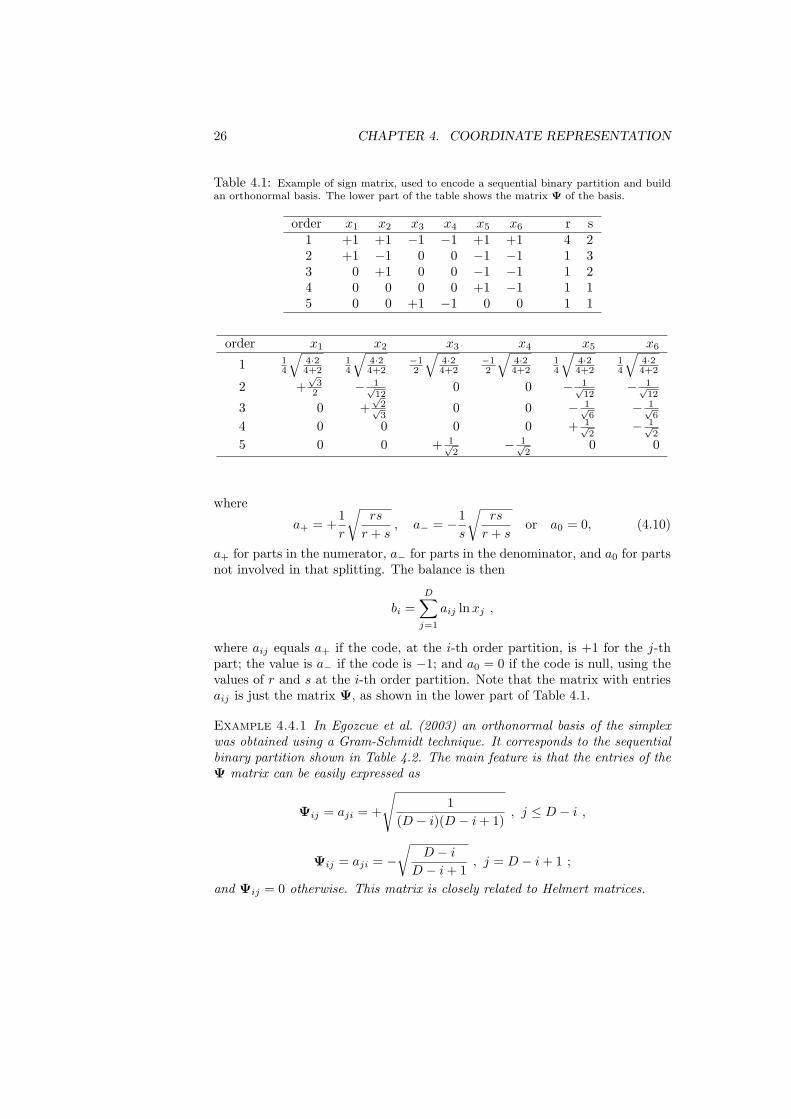
There are several ways to define orthonormal bases in the simplex. The maincriterion for the selection of an orthonormal basis is that it enhances the inter-pretability of the representation in coordinates. For instance, when performingprincipal component analysis an orthogonal basis is selected so that the first co-ordinate (principal component) represents the direction of maximum variability,etc. Particular cases deserving our attention are those bases linked to a se-quential binary partition of the compositional vector (Egozcue and Pawlowsky-Glahn, 2005). The main interest of such bases is that they are easily interpretedin terms of grouped parts of the composition. The Cartesian coordinates of acomposition in such a basis are called balances and the compositions of the basisbalancing elements. A sequential binary partition is a hierarchy of the parts ofa composition. In the first order of the hierarchy, all parts are split into twogroups. In the following steps, each group is in turn split into two groups, andthe process continues until all groups have a single part, as illustrated in Table4.1. For each order of the partition, it is possible to define the balance betweenthe two sub-groups formed at that level: if i1, i2, . . . , ir are the r parts of thefirst sub-group (coded by +1), and j1, j2, . . . , js the s parts of the second (codedby −1), the balance is defined as the normalised logratio of the geometric meanof each group of parts:
b =√
rs
r + sln
(xi1xi2 · · ·xir )1/r
(xj1xj2 · · ·xjs)1/s
= ln(xi1xi2 · · ·xir )
a+
(xj1xj2 · · ·xjs)a− , (4.9)
26 CHAPTER 4. COORDINATE REPRESENTATION
Table 4.1: Example of sign matrix, used to encode a sequential binary partition and buildan orthonormal basis. The lower part of the table shows the matrix Ψ of the basis.
order x1 x2 x3 x4 x5 x6 r s1 +1 +1 −1 −1 +1 +1 4 22 +1 −1 0 0 −1 −1 1 33 0 +1 0 0 −1 −1 1 24 0 0 0 0 +1 −1 1 15 0 0 +1 −1 0 0 1 1
order x1 x2 x3 x4 x5 x6
1 14
√4·24+2
14
√4·24+2
−12
√4·24+2
−12
√4·24+2
14
√4·24+2
14
√4·24+2
2 +√
32 − 1√
120 0 − 1√
12− 1√
12
3 0 +√
2√3
0 0 − 1√6
− 1√6
4 0 0 0 0 + 1√2
− 1√2
5 0 0 + 1√2
− 1√2
0 0
where
a+ = +1r
√rs
r + s, a− = −1
s
√rs
r + sor a0 = 0, (4.10)
a+ for parts in the numerator, a− for parts in the denominator, and a0 for partsnot involved in that splitting. The balance is then
bi =D∑
j=1
aij ln xj ,
where aij equals a+ if the code, at the i-th order partition, is +1 for the j-thpart; the value is a− if the code is −1; and a0 = 0 if the code is null, using thevalues of r and s at the i-th order partition. Note that the matrix with entriesaij is just the matrix Ψ, as shown in the lower part of Table 4.1.
Example 4.4.1 In Egozcue et al. (2003) an orthonormal basis of the simplexwas obtained using a Gram-Schmidt technique. It corresponds to the sequentialbinary partition shown in Table 4.2. The main feature is that the entries of theΨ matrix can be easily expressed as
Ψij = aji = +
√1
(D − i)(D − i + 1), j ≤ D − i ,
Ψij = aji = −√
D − i
D − i + 1, j = D − i + 1 ;
and Ψij = 0 otherwise. This matrix is closely related to Helmert matrices.
4.4. ORTHONORMAL COORDINATES 27
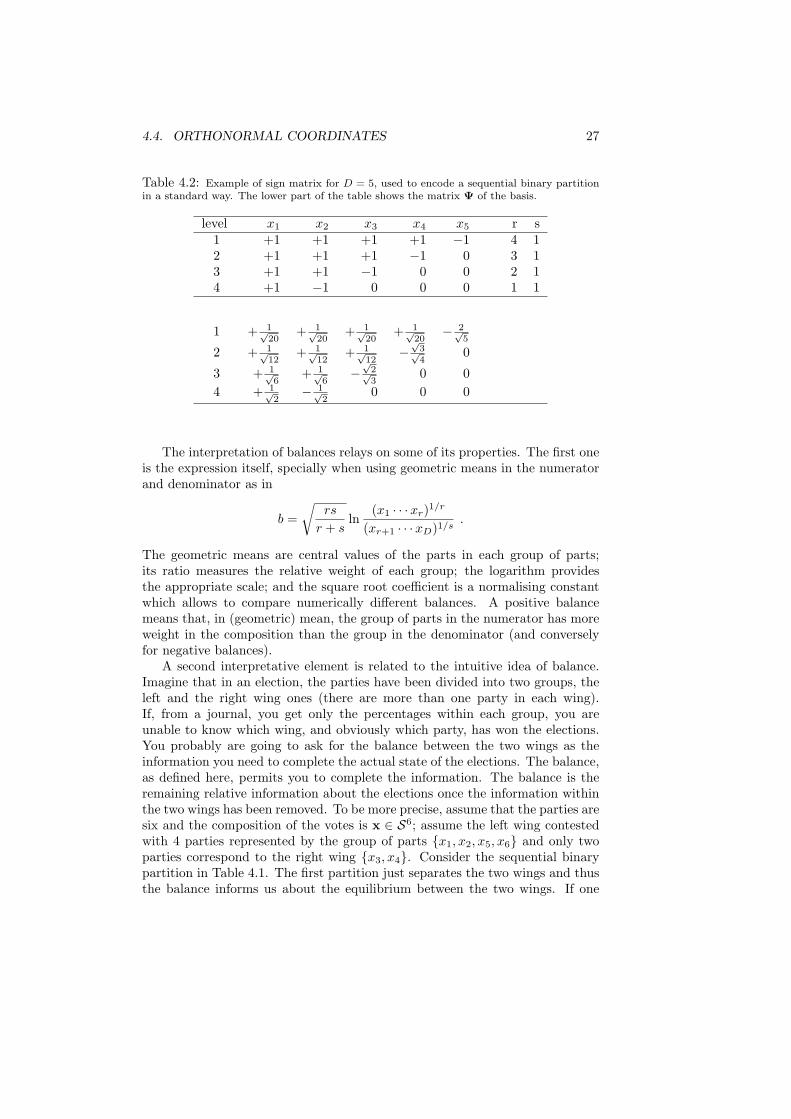
Table 4.2: Example of sign matrix for D = 5, used to encode a sequential binary partitionin a standard way. The lower part of the table shows the matrix Ψ of the basis.
level x1 x2 x3 x4 x5 r s1 +1 +1 +1 +1 −1 4 12 +1 +1 +1 −1 0 3 13 +1 +1 −1 0 0 2 14 +1 −1 0 0 0 1 1
1 + 1√20
+ 1√20
+ 1√20
+ 1√20
− 2√5
2 + 1√12
+ 1√12
+ 1√12
−√
3√4
0
3 + 1√6
+ 1√6
−√
2√3
0 04 + 1√
2− 1√
20 0 0
The interpretation of balances relays on some of its properties. The first oneis the expression itself, specially when using geometric means in the numeratorand denominator as in
b =√
rs
r + sln
(x1 · · ·xr)1/r
(xr+1 · · ·xD)1/s.
The geometric means are central values of the parts in each group of parts;its ratio measures the relative weight of each group; the logarithm providesthe appropriate scale; and the square root coefficient is a normalising constantwhich allows to compare numerically different balances. A positive balancemeans that, in (geometric) mean, the group of parts in the numerator has moreweight in the composition than the group in the denominator (and converselyfor negative balances).
A second interpretative element is related to the intuitive idea of balance.Imagine that in an election, the parties have been divided into two groups, theleft and the right wing ones (there are more than one party in each wing).If, from a journal, you get only the percentages within each group, you areunable to know which wing, and obviously which party, has won the elections.You probably are going to ask for the balance between the two wings as theinformation you need to complete the actual state of the elections. The balance,as defined here, permits you to complete the information. The balance is theremaining relative information about the elections once the information withinthe two wings has been removed. To be more precise, assume that the parties aresix and the composition of the votes is x ∈ S6; assume the left wing contestedwith 4 parties represented by the group of parts {x1, x2, x5, x6} and only twoparties correspond to the right wing {x3, x4}. Consider the sequential binarypartition in Table 4.1. The first partition just separates the two wings and thusthe balance informs us about the equilibrium between the two wings. If one
28 CHAPTER 4. COORDINATE REPRESENTATION
leaves out this balance, the remaining balances inform us only about the leftwing (balances 3,4) and only about the right wing (balance 5). Therefore, toretain only balance 5 is equivalent to know the relative information within thesubcomposition called right wing. Similarly, balances 2, 3 and 4 only informabout what happened within the left wing. The conclusion is that the balance1, the forgotten information in the journal, does not inform us about relationswithin the two wings: it only conveys information about the balance betweenthe two groups representing the wings.
Many questions can be stated which can be handled easily using the balances.For instance, suppose we are interested in the relationships between the partieswithin the left wing and, consequently, we want to remove the informationwithin the right wing. A traditional approach to this is to remove parts x3 andx4 and then close the remaining subcomposition. However, this is equivalentto project the composition of 6 parts orthogonally onto the subspace associatedwith the left wing, what is easily done by setting b5 = 0. If we do so, theobtained projected composition is
xproj = C[x1, x2, g(x3, x4), g(x3, x4), x5, x6] , g(x3, x4) = (x3x4)1/2 ,
i.e. each part in the right wing has been substituted by the geometric meanwithin the right wing. This composition still has the information on the left-right balance, b1. If we are also interested in removing it (b1 = 0), the remaininginformation will be only that within the left-wing subcomposition which is rep-resented by the orthogonal projection
xleft = C[x1, x2, g(x1, x2, x5, x6), g(x1, x2, x5, x6), x5, x6] ,
with g(x1, x2, x5, x6) = (x1, x2, x5, x6)1/4. The conclusion is that the balancescan be very useful to project compositions onto special subspaces just by re-taining some balances and making other ones null.
4.5 Working in coordinates
Coordinates with respect to an orthonormal basis in a linear vector space un-derly standard rules of operation in real space. As a consequence, perturbationin SD is equivalent to translation in real space, and power transformation inSD is equivalent to multiplication. Thus, if we consider the vector of coordi-nates h(x) = x∗ ∈ RD−1 of a compositional vector x ∈ SD with respect to anarbitrary orthonormal basis, it holds (Property 4.4.1)
h(x⊕ y) = h(x) + h(y) = x∗ + y∗ , h(α¯ x) = α · h(x) = α · x∗ , (4.11)
and we can think about perturbation as having the same properties in thesimplex as translation has in real space, and of the power transformation ashaving the same properties as multiplication.
Furthermore,
da(x,y) = d(h(x), h(y)) = d(x∗,y∗),
4.5. WORKING IN COORDINATES 29
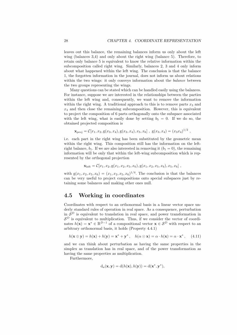
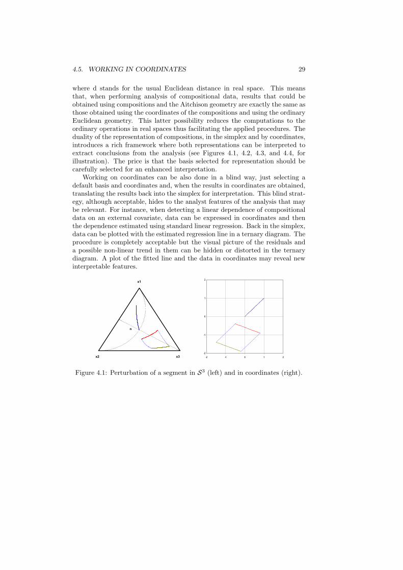
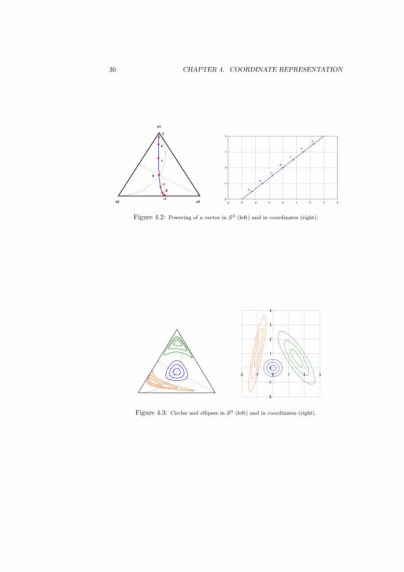
where d stands for the usual Euclidean distance in real space. This meansthat, when performing analysis of compositional data, results that could beobtained using compositions and the Aitchison geometry are exactly the same asthose obtained using the coordinates of the compositions and using the ordinaryEuclidean geometry. This latter possibility reduces the computations to theordinary operations in real spaces thus facilitating the applied procedures. Theduality of the representation of compositions, in the simplex and by coordinates,introduces a rich framework where both representations can be interpreted toextract conclusions from the analysis (see Figures 4.1, 4.2, 4.3, and 4.4, forillustration). The price is that the basis selected for representation should becarefully selected for an enhanced interpretation.
Working on coordinates can be also done in a blind way, just selecting adefault basis and coordinates and, when the results in coordinates are obtained,translating the results back into the simplex for interpretation. This blind strat-egy, although acceptable, hides to the analyst features of the analysis that maybe relevant. For instance, when detecting a linear dependence of compositionaldata on an external covariate, data can be expressed in coordinates and thenthe dependence estimated using standard linear regression. Back in the simplex,data can be plotted with the estimated regression line in a ternary diagram. Theprocedure is completely acceptable but the visual picture of the residuals anda possible non-linear trend in them can be hidden or distorted in the ternarydiagram. A plot of the fitted line and the data in coordinates may reveal newinterpretable features.
x2
x1
x3
n
-2
-1
0
1
2
-2 -1 0 1 2
Figure 4.1: Perturbation of a segment in S3 (left) and in coordinates (right).
30 CHAPTER 4. COORDINATE REPRESENTATION
x2
x1
x3
0
-1
-2
1
2
-3
3
-2
-1
0
1
2
-4 -3 -2 -1 0 1 2 3 4
-3
-2
-1
0
1
2
3
Figure 4.2: Powering of a vector in S3 (left) and in coordinates (right).
-2
-1
0
1
2
3
4
-2 -1 0 1 2 3
Figure 4.3: Circles and ellipses in S3 (left) and in coordinates (right).
4.6. ADDITIVE LOG-RATIO COORDINATES 31
x2
x1
x3
n
-4
-2
0
2
4
-4 -2 0 2 4
Figure 4.4: Couples of parallel lines in S3 (left) and in coordinates (right).
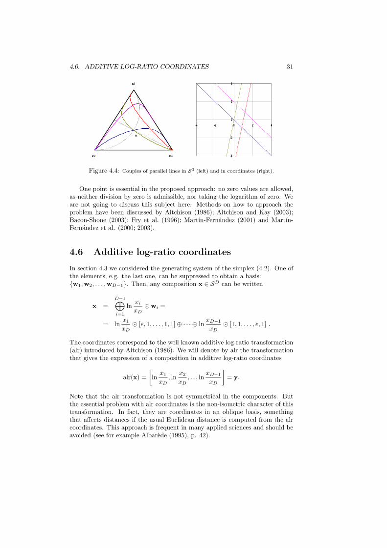
One point is essential in the proposed approach: no zero values are allowed,as neither division by zero is admissible, nor taking the logarithm of zero. Weare not going to discuss this subject here. Methods on how to approach theproblem have been discussed by Aitchison (1986); Aitchison and Kay (2003);Bacon-Shone (2003); Fry et al. (1996); Martın-Fernandez (2001) and Martın-Fernandez et al. (2000; 2003).
4.6 Additive log-ratio coordinates
In section 4.3 we considered the generating system of the simplex (4.2). One ofthe elements, e.g. the last one, can be suppressed to obtain a basis:{w1,w2, . . . ,wD−1}. Then, any composition x ∈ SD can be written
x =D−1⊕
i=1
lnxi
xD¯wi =
= lnx1
xD¯ [e, 1, . . . , 1, 1]⊕ · · · ⊕ ln
xD−1
xD¯ [1, 1, . . . , e, 1] .
The coordinates correspond to the well known additive log-ratio transformation(alr) introduced by Aitchison (1986). We will denote by alr the transformationthat gives the expression of a composition in additive log-ratio coordinates
alr(x) =[ln
x1
xD, ln
x2
xD, ..., ln
xD−1
xD
]= y.
Note that the alr transformation is not symmetrical in the components. Butthe essential problem with alr coordinates is the non-isometric character of thistransformation. In fact, they are coordinates in an oblique basis, somethingthat affects distances if the usual Euclidean distance is computed from the alrcoordinates. This approach is frequent in many applied sciences and should beavoided (see for example Albarede (1995), p. 42).
32 CHAPTER 4. COORDINATE REPRESENTATION
4.7 Simplicial matrix notation
Many operations in real spaces are expressed in matrix notation. Since thesimplex is an Euclidean space, matrix notations may be also useful. However,in this framework a vector of real constants cannot be considered in the simplexalthough in the real space they are readily identified. This produces two kindof matrix products which are introduced in this section. The first is simply theexpression of a perturbation-linear combination of compositions which appearsas a power-multiplication of a real vector by a compositional matrix whose rowsare in the simplex. The second one is the expression of a linear transformation inthe simplex: a composition is transformed by a matrix, involving perturbationand powering, to obtain a new composition. The real matrix implied in this caseis not a general one but when expressed in coordinates it is completely general.
Perturbation-linear combination of compositions
For a row vector of ` scalars a = [a1, a2, . . . , a`] and an array of row vectorsV = (v1,v2, . . . ,v`)
′, i.e. an (`,D)-matrix,
a¯V = [a1, a2, . . . , a`]¯
v1
v2
...v`
= [a1, a2, . . . , a`]¯
v11 v12 · · · v1D
v21 v22 · · · v2D
......
. . ....
v`1 v`2 · · · v`D
=
⊕
i=1
ai ¯ vi.
The components of this matrix product are
a¯V = C∏
j=1
vaj
j1 ,∏
j=1
vaj
j2 , . . . ,∏
j=1
vaj
jD
.
In coordinates this simplicial matrix product takes the form of a linear com-bination of the coordinate vectors. In fact, if h is the function assigning thecoordinates,
h(a¯V) = h
(⊕
i=1
ai ¯ vi
)=
∑
i=1
ai h(vi) .
Example 4.7.1 A composition in SD can be expressed as a perturbation-linearcombination of the elements of the basis ei, i = 1, 2, . . . , D − 1 as in Equation(4.6). Consider the (D− 1, D)-matrix E = (e1, e2, . . . , eD−1)′ and the vector ofcoordinates x∗ = ilr(x). Equation (4.6) can be re-written as
x = x∗ ¯E .
4.7. SIMPLICIAL MATRIX NOTATION 33
Perturbation-linear transformation of SD: endomorphisms
Consider a row vector of coordinates x∗ ∈ RD−1 and a general (D − 1, D − 1)-matrix A∗. In the real space setting, y∗ = x∗A∗ expresses an endomorphism,obviously linear in the real sense. Given the isometric isomorphism of the realspace of coordinates onto the simplex, the A∗ endomorphism has an expressionin the simplex. Taking ilr−1 = h−1 in the expression of the real endomorphismand using Equation (4.8)
y = C(exp[x∗A∗Ψ]) = C(exp[clr(x)Ψ′A∗Ψ]) (4.12)
where Ψ is the clr matrix of the selected basis and the right-most member hasbeen obtained applying Equation (4.7) to x∗. The (D, D)-matrix A = Ψ′A∗Ψhas entries
aij =D−1∑
k=1
D−1∑m=1
ΨkiΨmja∗km , i, j = 1, 2, . . . , D .
Substituting clr(x) by its expression as a function of the logarithms of parts,the composition y is
y = C
D∏
j=1
xaj1j ,
D∏
j=1
xaj2j , . . . ,
D∏
j=1
xajD
j
,
which, taking into account that products and powers match the definitions of⊕ and ¯, deserves the definition
y = x ◦A = x ◦ (Ψ′A∗Ψ) , (4.13)
where ◦ is the perturbation-matrix product representing an endomorphism inthe simplex. This matrix product in the simplex should not be confused withthat defined between a vector of scalars and a matrix of compositions and de-noted by ¯.
An important conclusion is that endomorphisms in the simplex are repre-sented by matrices with a peculiar structure given by A = Ψ′A∗Ψ, which havesome remarkable properties:
(a) it is a (D, D) real matrix;
(b) each row and each column of A adds to 0;
(c) rank(A) = rank(A∗); particularly, when A∗ is full-rank, rank(A) = D− 1;
(d) the identity endomorphism corresponds to A∗ = ID−1, the identity inRD−1, and to A = Ψ′Ψ = ID − (1/D)1′D1D, where ID is the identity(D,D)-matrix, and 1D is a row vector of ones.
34 CHAPTER 4. COORDINATE REPRESENTATION
The matrix A∗ can be recovered from A as A∗ = ΨAΨ′. However, A isnot the only matrix corresponding to A∗ in this transformation. Consider thefollowing (D, D)-matrix
A = A0 +D∑
i=1
ci(~ei)′1D +D∑
j=1
dj1′D~ej ,
where, A0 satisfies the above conditions, ~ei = [0, 0, . . . , 1, . . . , 0, 0] is the i-throw-vector in the canonical basis of RD, and ci, dj are arbitrary constants.Each additive term in this expression adds a constant row or column, beingthe remaining entries null. A simple development proves that A∗ = ΨAΨ′ =ΨA0Ψ′. This means that x ◦ A = x ◦ A0, i.e. A, A0 define the same lineartransformation in the simplex. To obtain A0 from A, first compute A∗ = ΨAΨ′
and then compute
A0 = Ψ′A∗Ψ = Ψ′ΨAΨ′Ψ = (ID − (1/D)1′D1D)A(ID − (1/D)1′D1D) ,
where the second member is the required computation and the third memberexplains that the computation is equivalent to add constant rows and columnsto A.
Example 4.7.2 Consider the matrix
A =(
0 a2
a1 0
)
representing a linear transformation in S2. The matrix Ψ is
Ψ =[
1√2,− 1√
2
].
In coordinates, this corresponds to a (1, 1)-matrix A∗ = (−(a1 + a2)/2). Theequivalent matrix A0 = Ψ′A∗Ψ is
A0 =( −a1+a2
4a1+a2
4a1+a2
4 −a1+a24
),
whose columns and rows add to 0.
4.8 Exercises
Exercise 4.8.1 Consider the data set given in Table 2.1. Compute the clrcoefficients (Eq. 4.3) to compositions with no zeros. Verify that the sum of thetransformed components equals zero.
Exercise 4.8.2 Using the sign matrix of Table 4.1 and Equation (4.10), com-pute the coefficients for each part at each level. Arrange them in a 6×5 matrix.Which are the vectors of this basis?
4.8. EXERCISES 35
Exercise 4.8.3 Consider the 6-part composition
[x1, x2, x3, x4, x5, x6] = [3.74, 9.35, 16.82, 18.69, 23.36, 28.04] % .
Using the binary partition of Table 4.1 and Eq. (4.9), compute its 5 balances.Compare with what you obtained in the preceding exercise.
Exercise 4.8.4 Consider the log-ratios c1 = lnx1/x3 and c2 = ln x2/x3 in asimplex S3. They are coordinates when using the alr transformation. Find twounitary vectors e1 and e2 such that 〈x, ei〉a = ci, i = 1, 2. Compute the innerproduct 〈e1, e2〉a and determine the angle between them. Does the result changeif the considered simplex is S7?
Exercise 4.8.5 When computing the clr of a composition x ∈ SD, a clr coeffi-cient is ξi = ln(xi/g(x)). This can be consider as a balance between two groupsof parts, which are they and which is the corresponding balancing element?
Exercise 4.8.6 Six parties have contested elections. In five districts they haveobtained the votes in Table 4.3. Parties are divided into left (L) and right (R)wings. Is there some relationship between the L-R balance and the relative votesof R1-R2? Select an adequate sequential binary partition to analyse this questionand obtain the corresponding balance coordinates. Find the correlation matrix ofthe balances and give an interpretation to the maximum correlated two balances.Compute the distances between the five districts; which are the two districts withthe maximum and minimum inter-distance. Are you able to distinguish somecluster of districts?
Table 4.3: Votes obtained by six parties in five districts.
L1 L2 R1 R2 L3 L4d1 10 223 534 23 154 161d2 43 154 338 43 120 123d3 3 78 29 702 265 110d4 5 107 58 598 123 92d5 17 91 112 487 80 90
Exercise 4.8.7 Consider the data set given in Table 2.1. Check the data forzeros. Apply the alr transformation to compositions with no zeros. Plot thetransformed data in R2.
Exercise 4.8.8 Consider the data set given in table 2.1 and take the compo-nents in a different order. Apply the alr transformation to compositions with nozeros. Plot the transformed data in R2. Compare the result with those obtainedin Exercise 4.8.7.

36 CHAPTER 4. COORDINATE REPRESENTATION
Exercise 4.8.9 Consider the data set given in table 2.1. Apply the ilr trans-formation to compositions with no zeros. Plot the transformed data in R2.Compare the result with the scatterplots obtained in exercises 4.8.7 and 4.8.8using the alr transformation.
Exercise 4.8.10 Compute the alr and ilr coordinates, as well as the clr coeffi-cients of the 6-part composition
[x1, x2, x3, x4, x5, x6] = [3.74, 9.35, 16.82, 18.69, 23.36, 28.04]% .
Exercise 4.8.11 Consider the 6-part composition of the preceding exercise.Using the binary partition of Table 4.1 and Equation (4.9), compute its 5 bal-ances. Compare with the results of the preceding exercise.
Chapter 5
Exploratory data analysis
5.1 General remarks
In this chapter we are going to address the first steps that should be performedwhenever the study of a compositional data set X is initiated. Essentially, thesesteps are five. They consist in (1) computing descriptive statistics, i.e. thecentre and variation matrix of a data set, as well as its total variability; (2)centring the data set for a better visualisation of subcompositions in ternarydiagrams; (3) looking at the biplot of the data set to discover patterns; (4)defining an appropriate representation in orthonormal coordinates and comput-ing the corresponding coordinates; and (5) compute the summary statistics ofthe coordinates and represent the results in a balance-dendrogram. In general,the last two steps will be based on a particular sequential binary partition, de-fined either a priori or as a result of the insights provided by the precedingthree steps. The last step consist of a graphical representation of the sequentialbinary partition, including a graphical and numerical summary of descriptivestatistics of the associated coordinates.
Before starting, let us make some general considerations. The first thing instandard statistical analysis is to check the data set for errors, and we assumethis part has been already done using standard procedures (e.g. using theminimum and maximum of each component to check whether the values arewithin an acceptable range). Another, quite different thing is to check the dataset for outliers, a point that is outside the scope of this short-course. See Barceloet al. (1994, 1996) for details. Recall that outliers can be considered as suchonly with respect to a given distribution. Furthermore, we assume there areno zeros in our samples. Zeros require specific techniques (Aitchison and Kay,2003; Bacon-Shone, 2003; Fry et al., 1996; Martın-Fernandez, 2001; Martın-Fernandez et al., 2000; Martın-Fernandez et al., 2003) and will be addressed infuture editions of this short course.
37
38 CHAPTER 5. EXPLORATORY DATA ANALYSIS
5.2 Centre, total variance and variation matrix
Standard descriptive statistics are not very informative in the case of compo-sitional data. In particular, the arithmetic mean and the variance or standarddeviation of individual components do not fit with the Aitchison geometry asmeasures of central tendency and dispersion. The skeptic reader might con-vince himself/herself by doing exercise 5.8.1 immediately. These statistics weredefined as such in the framework of Euclidean geometry in real space, whichis not a sensible geometry for compositional data. Therefore, it is necessaryto introduce alternatives, which we find in the concepts of centre (Aitchison,1997), variation matrix, and total variance (Aitchison, 1986).
Definition 5.2.1 A measure of central tendency for compositional data is theclosed geometric mean. For a data set of size n it is called centre and is definedas
g = C [g1, g2, . . . , gD] ,
with gi = (∏n
j=1 xij)1/n, i = 1, 2, . . . , D.
Note that in the definition of centre of a data set the geometric mean isconsidered column-wise (i.e. by parts), while in the clr transformation, given inequation (4.3), the geometric mean is considered row-wise (i.e. by samples).
Definition 5.2.2 Dispersion in a compositional data set can be described eitherby the variation matrix, originally defined by Aitchison (1986) as
T =
t11 t12 · · · t1D
t21 t22 · · · t2D
......
. . ....
tD1 tD2 · · · tDD
, tij = var
(ln
xi
xj
),
or by the normalised variation matrix
T∗ =
t∗11 t∗12 · · · t∗1D
t∗21 t∗22 · · · t∗2D...
.... . .
...t∗D1 t∗D2 · · · t∗DD
, t∗ij = var
(1√2
lnxi
xj
).
As can be seen, tij stands for the usual experimental variance of the log-ratioof parts i and j, while t∗ij stands for the usual experimental variance of thenormalised log-ratio of parts i and j, so that the log ratio is a balance.
Note that
t∗ij = var(
1√2
lnxi
xj
)=
12tij ,
and thus T∗ = 12T. Normalised variations have squared Aitchison distance
units (see Figure 3.3).
5.3. CENTRING AND SCALING 39
Definition 5.2.3 A measure of global dispersion is the total variance given by
totvar[X] =1
2D
D∑
i=1
D∑
j=1
var(
lnxi
xj
)=
12D
D∑
i=1
D∑
j=1
tij =1D
D∑
i=1
D∑
j=1
t∗ij .
By definition, T and T∗ are symmetric and their diagonal will contain onlyzeros. Furthermore, neither the total variance nor any single entry in bothvariation matrices depend on the constant κ associated with the sample spaceSD, as constants cancel out when taking ratios. Consequently, rescaling hasno effect. These statistics have further connections. From their definition, itis clear that the total variation summarises the variation matrix in a singlequantity, both in the normalised and non-normalised version, and it is possible(and natural) to define it because all parts in a composition share a commonscale (it is by no means so straightforward to define a total variation for apressure-temperature random vector, for instance). Conversely, the variationmatrix, again in both versions, explains how the total variation is split amongthe parts (or better, among all log-ratios).
5.3 Centring and scaling
A usual way in geology to visualise data in a ternary diagram is to rescale theobservations in such a way that their range is approximately the same. Thisis nothing else but applying a perturbation to the data set, a perturbationwhich is usually chosen by trial and error. To overcome this somehow arbitraryapproach, note that, as mentioned in Proposition 3.2.1, for a composition x andits inverse x−1 it holds that x⊕x−1 = n, the neutral element. This means thatperturbation allows to move any composition to the barycentre of the simplex,in the same way that translation moves real data in real space to the origin.This property, together with the definition of centre, allows to design a strategyto better visualise the structure of the sample. In fact, computing the centre gof the data set, as in Definition 5.2.1, and perturbing each sample compositionby the inverse g−1, the centre of a data set is shifted to the barycentre of thesimplex, and the sample will gravitate around the barycentre.
This property was first introduced by Martın-Fernandez et al. (1999) andused by Buccianti et al. (1999). An extensive discussion can be found in von Ey-natten et al. (2002), where it is shown that a perturbation transforms straightlines into straight lines. This allows the inclusion of gridlines and compositionalfields in the graphical representation without the risk of a nonlinear distortion.See Figure 5.1 for an example of a data set before and after perturbation withthe inverse of the closed geometric mean and the effect on the gridlines.
In the same way in real space a centred variable can be scaled to unit variancedividing it by the standard deviation, a (centred) compositional data set X canbe scaled by powering it with totvar[X]−1/2. In this way, a data set with unittotal variance is obtained, but with the same relative contribution of each log-ratio in the variation array. This is a significant difference with conventional
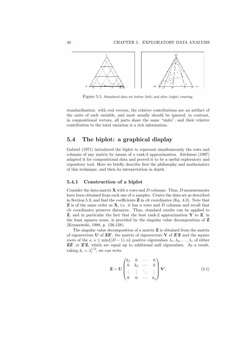
40 CHAPTER 5. EXPLORATORY DATA ANALYSIS
Figure 5.1: Simulated data set before (left) and after (right) centring.
standardisation: with real vectors, the relative contributions are an artifact ofthe units of each variable, and most usually should be ignored; in contrast,in compositional vectors, all parts share the same “units”, and their relativecontribution to the total variation is a rich information.
5.4 The biplot: a graphical display
Gabriel (1971) introduced the biplot to represent simultaneously the rows andcolumns of any matrix by means of a rank-2 approximation. Aitchison (1997)adapted it for compositional data and proved it to be a useful exploratory andexpository tool. Here we briefly describe first the philosophy and mathematicsof this technique, and then its interpretation in depth.
5.4.1 Construction of a biplot
Consider the data matrix X with n rows and D columns. Thus, D measurementshave been obtained from each one of n samples. Centre the data set as describedin Section 5.3, and find the coefficients Z in clr coordinates (Eq. 4.3). Note thatZ is of the same order as X, i.e. it has n rows and D columns and recall thatclr coordinates preserve distances. Thus, standard results can be applied toZ, and in particular the fact that the best rank-2 approximation Y to Z, inthe least squares sense, is provided by the singular value decomposition of Z(Krzanowski, 1988, p. 126-128).
The singular value decomposition of a matrix Z is obtained from the matrixof eigenvectors U of ZZ′, the matrix of eigenvectors V of Z′Z and the squareroots of the s, s ≤ min{(D − 1), n} positive eigenvalues λ1, λ2, . . . , λs of eitherZZ′ or Z′Z, which are equal up to additional null eigenvalues. As a result,taking ki = λ
1/2i , we can write
Z = U
k1 0 · · · 00 k2 · · · 0...
.... . .
...0 0 · · · ks
V′, (5.1)
5.4. THE BIPLOT: A GRAPHICAL DISPLAY 41
where s is the rank of Z and the singular values k1, k2, . . . , ks are in descendingorder of magnitude. The matrix U has dimensions (n, s) and V is a (D, s)-matrix. Both matrices U and V are orthonormal, i.e. UU′ = Is, VV′ = Is.When Z is made of centered clr’s of compositional data, its rows add to zeroand consequently its rank is s ≤ D − 1 being the common case s = D − 1.The interpretation of SVD (5.1) is straightforward. Each row of matrix V′
is the clr of an element of an orthonormal basis of the simplex. This kind ofmatrices have been denoted Ψ in chapter 4, section 4.4. The matrix productU diag(k1, k2, · · · , ks) is an (n, s)-matrix whose n rows contain the coordinatesof each compositional data point with respect to the orthonormal basis de-scribed by V′. Therefore, U diag(k1, k2, · · · , ks) contains ilr-coordinates of the(centered)-compositional data set. Note that these ilr-coordinates are not bal-ances but general orthonormal coordinates. Singular values λ1 = k2
1, λ2 = k22,
. . . , λs = k2s , are proportional to the sample variance of the coordinates.
In order to reduce the dimension of the compositional data set, we can sup-press some orthogonal coordinates, typically those with associated low variance.This can be thought as a deletion of small square-singular values. Assume thatwe retain singular values k1, k2, . . . , kt, (t ≤ s). Then the proportion of retainedvariance is
k21 + k2
2 + · · ·+ k2t
k21 + k2
2 + · · ·+ k2s
=λ1 + λ2 + · · ·+ λt
λ1 + λ2 + · · ·+ λs.
The biplot is normally drawn in two dimensions, or at most three dimensions,and then we normally take t = 2, provided that the proportion of explainedvariance is high. This rank-2 approximation is then obtained by simply substi-tuting all singular values with index larger then 2 by zero. As a result we get arank-2 approximation of Z
Y =
u11 u21
u12 u22
......
u1n u2n
(k1 00 k2
)(v11 v21 · · · vD1
v12 v22 · · · vD2
). (5.2)
The proportion of variability retained by this approximation is (λ1+λ2)/(∑s
i=1 λi) .To obtain a biplot, it is first necessary to write Y as the product of two
matrices GH′, where G is an (n, 2) matrix and H is an (D, 2) matrix. Thereare different possibilities to obtain such a factorisation, one of which is
Y =
√n u11
√n u21√
n u12√
n u22
......√
n u1n√
n u2n
(k1v11√
nk1v21√
n· · · k1vD1√
nk2v12√
nk2v22√
n· · · k2vD2√
n
)
=
g1
g2
...gn
(h1 h2 · · · hD
).
42 CHAPTER 5. EXPLORATORY DATA ANALYSIS
The biplot consists simply in representing the vectors gi, i = 1, 2, ..., n (rowvectors of two components), and hj , j = 1, 2, ..., D (column vectors of twocomponents), on a plane. The vectors g1, g2, ..., gn are termed the row markersof Y and correspond to the projections of the n samples on the plane definedby the first two eigenvectors of ZZ′. The vectors h1, h2, ..., hD are the columnmarkers, which correspond to the projections of the D clr-parts on the planedefined by the first two eigenvectors of Z′Z. Both planes can be superposed fora visualisation of the relationship between samples and parts.
5.4.2 Interpretation of a compositional biplot
The biplot graphically displays the rank-2 approximation Y to Z given by thesingular value decomposition. A biplot of compositional data consists of
1. an origin O which represents the centre of the compositional data set,
2. a vertex at position hj for each of the D parts, and
3. a case marker at position gi for each of the n samples or cases.
We term the join of O to a vertex hj the ray Ohj and the join of two verticeshj and hk the link hjhk. These features constitute the basic characteristics of abiplot with the following main properties for the interpretation of compositionalvariability.
1. Links and rays provide information on the relative variability in a compo-sitional data set, as
|hjhk|2 ≈ var(
lnxj
xk
)and |Ohj |2 ≈ var
(ln
xj
g(x)
).
Nevertheless, one has to be careful in interpreting rays, which cannotbe identified neither with var(xj) nor with var(lnxj), as they depend onthe full composition through g(x) and vary when a subcomposition isconsidered.
2. Links provide information on the correlation of subcompositions: if linkshjhk and hih` intersect at M then
cos(hjMhi) ≈ corr(
lnxj
xk, ln
xi
x`
).
Furthermore, if the two links are at right angles, then cos(hjMhi) ≈ 0,and zero correlation of the two log-ratios can be expected. This is usefulin investigation of subcompositions for possible independence.
3. Subcompositional analysis: The centre O is the centroid (centre of gravity)of the D vertices h1,h2, . . . ,hD; ratios are preserved under formationof subcompositions; it follows that the biplot for any subcomposition is
5.5. EXPLORATORY ANALYSIS OF COORDINATES 43
simply formed by selecting the vertices corresponding to the parts of thesubcomposition and taking the centre of the subcompositional biplot asthe centroid of these vertices.
4. Coincident vertices: If vertices hj and hk coincide, or nearly so, this meansthat var(ln(xj/xk)) is zero, or nearly so, and the ratio xj/xk is constant,or nearly so. Then, the two involved parts, xj and xk can be assumed tobe redundant. If the proportion of variance captured by the biplot is notvery high, two coincident vertices suggest that ln(xj/xk) is orthogonal tothe plane of the biplot, and this might be an indication of the possibleindependence of that log-ratio and the two first principal directions of thesingular value decomposition.
5. Collinear vertices: If a subset of vertices is collinear, it might indicate thatthe associated subcomposition has a biplot that is one-dimensional, whichmight mean that the subcomposition has one-dimensional variability, i.e.compositions plot along a compositional line.
From the above aspects of interpretation, it should be clear that links arefundamental elements of a compositional biplot. The lengths of links are (ap-proximately) proportional to variance of simple log-ratios between single ele-ments, as they appear in the variation matrix. The complete constellation oflinks informs about the compositional covariance structure of simple log-ratiosand provides hints about subcompositional variability and independence. Inter-pretation of the biplot is concerned with its internal geometry and is unaffectedby any rotation or mirror-imaging of the diagram. For an illustration, see Sec-tion 5.6.
For some applications of biplots to compositional data in a variety of ge-ological contexts see Aitchison (1990), and for a deeper insight into biplotsof compositional data, with applications in other disciplines and extensions toconditional biplots, see Aitchison and Greenacre (2002).
5.5 Exploratory analysis of coordinates
Either as a result of the preceding descriptive analysis, or due to a priori knowl-edge of the problem at hand, we may consider a given sequential binary partitionas particularly interesting. In this case, its associated orthonormal coordinates,being a vector of real variables, can be treated with the existing battery of con-ventional descriptive analysis. If X∗ = h(X) represents the coordinates of thedata set—rows contain the coordinates of an individual observation—then itsexperimental moments satisfy
y∗ = h(g) = Ψ · clr(g) = Ψ · ln(g)Sy = −Ψ ·T∗ ·Ψ′
with Ψ the matrix whose rows contain the clr coefficients of the orthonormalbasis chosen (see Section 4.4 for its construction); g the centre of the dataset as
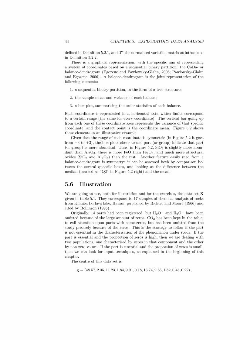
44 CHAPTER 5. EXPLORATORY DATA ANALYSIS
defined in Definition 5.2.1, and T∗ the normalised variation matrix as introducedin Definition 5.2.2.
There is a graphical representation, with the specific aim of representinga system of coordinates based on a sequential binary partition: the CoDa- orbalance-dendrogram (Egozcue and Pawlowsky-Glahn, 2006; Pawlowsky-Glahnand Egozcue, 2006). A balance-dendrogram is the joint representation of thefollowing elements:
1. a sequential binary partition, in the form of a tree structure;
2. the sample mean and variance of each balance;
3. a box-plot, summarising the order statistics of each balance.
Each coordinate is represented in a horizontal axis, which limits correspondto a certain range (the same for every coordinate). The vertical bar going upfrom each one of these coordinate axes represents the variance of that specificcoordinate, and the contact point is the coordinate mean. Figure 5.2 showsthese elements in an illustrative example.
Given that the range of each coordinate is symmetric (in Figure 5.2 it goesfrom −3 to +3), the box plots closer to one part (or group) indicate that part(or group) is more abundant. Thus, in Figure 5.2, SiO2 is slightly more abun-dant than Al2O3, there is more FeO than Fe2O3, and much more structuraloxides (SiO2 and Al2O3) than the rest. Another feature easily read from abalance-dendrogram is symmetry: it can be assessed both by comparison be-tween the several quantile boxes, and looking at the difference between themedian (marked as “Q2” in Figure 5.2 right) and the mean.
5.6 Illustration
We are going to use, both for illustration and for the exercises, the data set Xgiven in table 5.1. They correspond to 17 samples of chemical analysis of rocksfrom Kilauea Iki lava lake, Hawaii, published by Richter and Moore (1966) andcited by Rollinson (1995).
Originally, 14 parts had been registered, but H2O+ and H2O− have beenomitted because of the large amount of zeros. CO2 has been kept in the table,to call attention upon parts with some zeros, but has been omitted from thestudy precisely because of the zeros. This is the strategy to follow if the partis not essential in the characterisation of the phenomenon under study. If thepart is essential and the proportion of zeros is high, then we are dealing withtwo populations, one characterised by zeros in that component and the otherby non-zero values. If the part is essential and the proportion of zeros is small,then we can look for input techniques, as explained in the beginning of thischapter.
The centre of this data set is
g = (48.57, 2.35, 11.23, 1.84, 9.91, 0.18, 13.74, 9.65, 1.82, 0.48, 0.22) ,
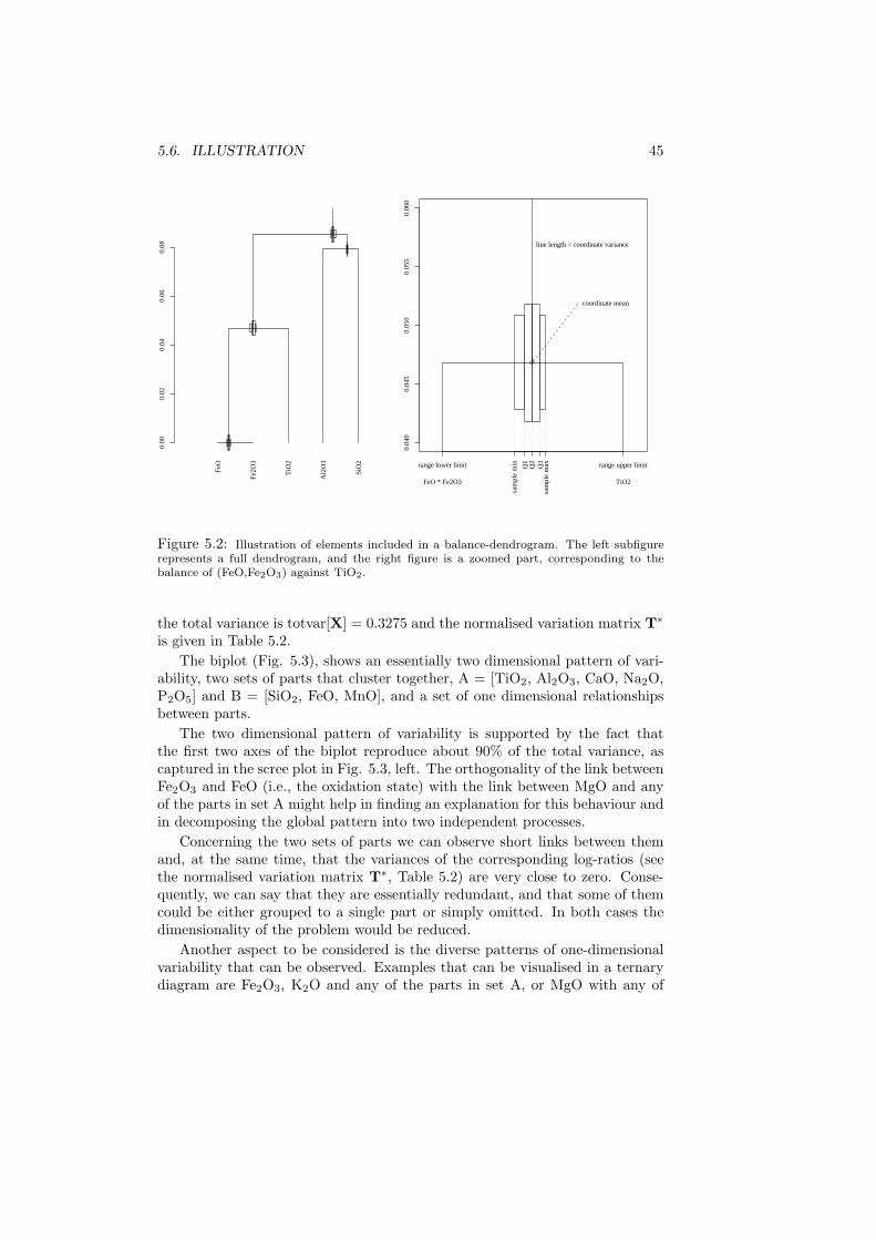
5.6. ILLUSTRATION 450.
000.
020.
040.
060.
08
FeO
Fe2O
3
TiO
2
Al2
O3
SiO
2
0.04
00.
045
0.05
00.
055
0.06
0
range lower limit range upper limit
FeO * Fe2O3 TiO2
sam
ple
min Q1
Q2
Q3
sam
ple
max
line length = coordinate variance
coordinate mean
Figure 5.2: Illustration of elements included in a balance-dendrogram. The left subfigurerepresents a full dendrogram, and the right figure is a zoomed part, corresponding to thebalance of (FeO,Fe2O3) against TiO2.
the total variance is totvar[X] = 0.3275 and the normalised variation matrix T∗
is given in Table 5.2.The biplot (Fig. 5.3), shows an essentially two dimensional pattern of vari-
ability, two sets of parts that cluster together, A = [TiO2, Al2O3, CaO, Na2O,P2O5] and B = [SiO2, FeO, MnO], and a set of one dimensional relationshipsbetween parts.
The two dimensional pattern of variability is supported by the fact thatthe first two axes of the biplot reproduce about 90% of the total variance, ascaptured in the scree plot in Fig. 5.3, left. The orthogonality of the link betweenFe2O3 and FeO (i.e., the oxidation state) with the link between MgO and anyof the parts in set A might help in finding an explanation for this behaviour andin decomposing the global pattern into two independent processes.
Concerning the two sets of parts we can observe short links between themand, at the same time, that the variances of the corresponding log-ratios (seethe normalised variation matrix T∗, Table 5.2) are very close to zero. Conse-quently, we can say that they are essentially redundant, and that some of themcould be either grouped to a single part or simply omitted. In both cases thedimensionality of the problem would be reduced.
Another aspect to be considered is the diverse patterns of one-dimensionalvariability that can be observed. Examples that can be visualised in a ternarydiagram are Fe2O3, K2O and any of the parts in set A, or MgO with any of
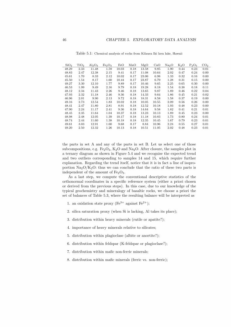
46 CHAPTER 5. EXPLORATORY DATA ANALYSIS
Table 5.1: Chemical analysis of rocks from Kilauea Iki lava lake, Hawaii
SiO2 TiO2 Al2O3 Fe2O3 FeO MnO MgO CaO Na2O K2O P2O5 CO2
48.29 2.33 11.48 1.59 10.03 0.18 13.58 9.85 1.90 0.44 0.23 0.0148.83 2.47 12.38 2.15 9.41 0.17 11.08 10.64 2.02 0.47 0.24 0.0045.61 1.70 8.33 2.12 10.02 0.17 23.06 6.98 1.33 0.32 0.16 0.0045.50 1.54 8.17 1.60 10.44 0.17 23.87 6.79 1.28 0.31 0.15 0.0049.27 3.30 12.10 1.77 9.89 0.17 10.46 9.65 2.25 0.65 0.30 0.0046.53 1.99 9.49 2.16 9.79 0.18 19.28 8.18 1.54 0.38 0.18 0.1148.12 2.34 11.43 2.26 9.46 0.18 13.65 9.87 1.89 0.46 0.22 0.0447.93 2.32 11.18 2.46 9.36 0.18 14.33 9.64 1.86 0.45 0.21 0.0246.96 2.01 9.90 2.13 9.72 0.18 18.31 8.58 1.58 0.37 0.19 0.0049.16 2.73 12.54 1.83 10.02 0.18 10.05 10.55 2.09 0.56 0.26 0.0048.41 2.47 11.80 2.81 8.91 0.18 12.52 10.18 1.93 0.48 0.23 0.0047.90 2.24 11.17 2.41 9.36 0.18 14.64 9.58 1.82 0.41 0.21 0.0148.45 2.35 11.64 1.04 10.37 0.18 13.23 10.13 1.89 0.45 0.23 0.0048.98 2.48 12.05 1.39 10.17 0.18 11.18 10.83 1.73 0.80 0.24 0.0148.74 2.44 11.60 1.38 10.18 0.18 12.35 10.45 1.67 0.79 0.23 0.0149.61 3.03 12.91 1.60 9.68 0.17 8.84 10.96 2.24 0.55 0.27 0.0149.20 2.50 12.32 1.26 10.13 0.18 10.51 11.05 2.02 0.48 0.23 0.01
the parts in set A and any of the parts in set B. Let us select one of thosesubcompositions, e.g. Fe2O3, K2O and Na2O. After closure, the samples plot ina ternary diagram as shown in Figure 5.4 and we recognise the expected trendand two outliers corresponding to samples 14 and 15, which require furtherexplanation. Regarding the trend itself, notice that it is in fact a line of isopro-portion Na2O/K2O: thus we can conclude that the ratio of these two parts isindependent of the amount of Fe2O3.
As a last step, we compute the conventional descriptive statistics of theorthonormal coordinates in a specific reference system (either a priori chosenor derived from the previous steps). In this case, due to our knowledge of thetypical geochemistry and mineralogy of basaltic rocks, we choose a priori theset of balances of Table 5.3, where the resulting balance will be interpreted as
1. an oxidation state proxy (Fe3+ against Fe2+);
2. silica saturation proxy (when Si is lacking, Al takes its place);
3. distribution within heavy minerals (rutile or apatite?);
4. importance of heavy minerals relative to silicates;
5. distribution within plagioclase (albite or anortite?);
6. distribution within feldspar (K-feldspar or plagioclase?);
7. distribution within mafic non-ferric minerals;
8. distribution within mafic minerals (ferric vs. non-ferric);
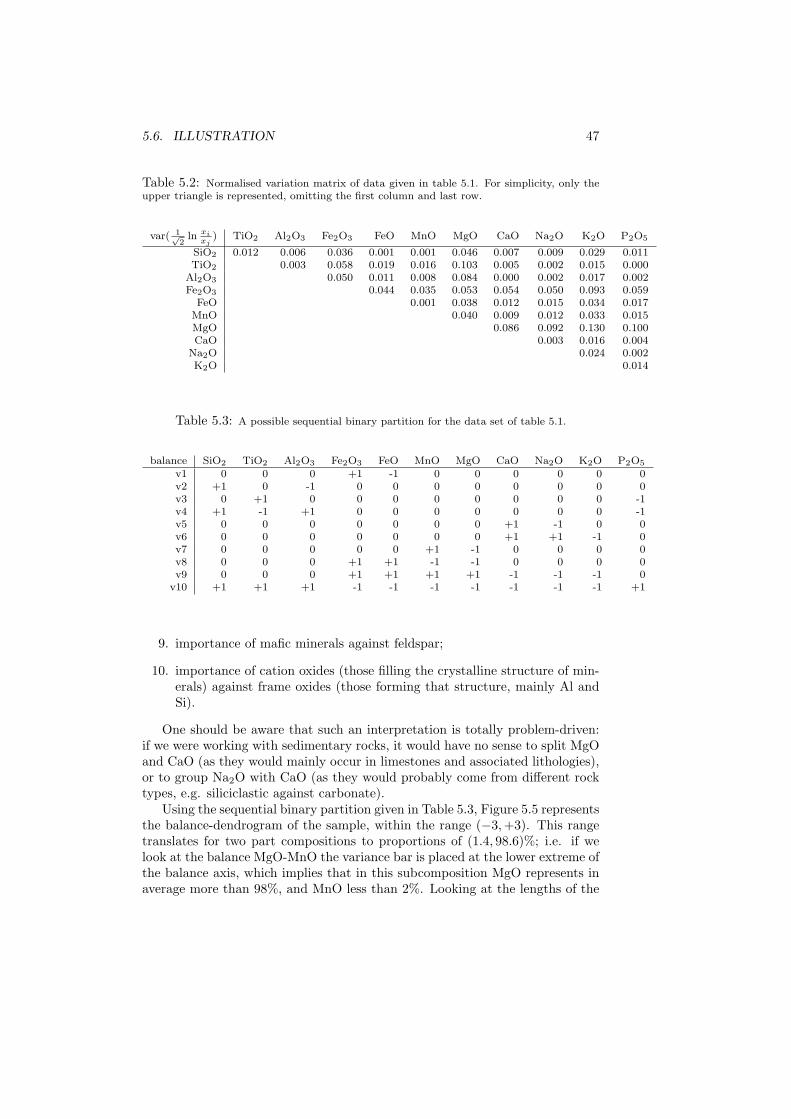
5.6. ILLUSTRATION 47
Table 5.2: Normalised variation matrix of data given in table 5.1. For simplicity, only theupper triangle is represented, omitting the first column and last row.
var( 1√2
ln xixj
) TiO2 Al2O3 Fe2O3 FeO MnO MgO CaO Na2O K2O P2O5
SiO2 0.012 0.006 0.036 0.001 0.001 0.046 0.007 0.009 0.029 0.011TiO2 0.003 0.058 0.019 0.016 0.103 0.005 0.002 0.015 0.000
Al2O3 0.050 0.011 0.008 0.084 0.000 0.002 0.017 0.002Fe2O3 0.044 0.035 0.053 0.054 0.050 0.093 0.059
FeO 0.001 0.038 0.012 0.015 0.034 0.017MnO 0.040 0.009 0.012 0.033 0.015MgO 0.086 0.092 0.130 0.100CaO 0.003 0.016 0.004
Na2O 0.024 0.002K2O 0.014
Table 5.3: A possible sequential binary partition for the data set of table 5.1.
balance SiO2 TiO2 Al2O3 Fe2O3 FeO MnO MgO CaO Na2O K2O P2O5
v1 0 0 0 +1 -1 0 0 0 0 0 0v2 +1 0 -1 0 0 0 0 0 0 0 0v3 0 +1 0 0 0 0 0 0 0 0 -1v4 +1 -1 +1 0 0 0 0 0 0 0 -1v5 0 0 0 0 0 0 0 +1 -1 0 0v6 0 0 0 0 0 0 0 +1 +1 -1 0v7 0 0 0 0 0 +1 -1 0 0 0 0v8 0 0 0 +1 +1 -1 -1 0 0 0 0v9 0 0 0 +1 +1 +1 +1 -1 -1 -1 0
v10 +1 +1 +1 -1 -1 -1 -1 -1 -1 -1 +1
9. importance of mafic minerals against feldspar;
10. importance of cation oxides (those filling the crystalline structure of min-erals) against frame oxides (those forming that structure, mainly Al andSi).
One should be aware that such an interpretation is totally problem-driven:if we were working with sedimentary rocks, it would have no sense to split MgOand CaO (as they would mainly occur in limestones and associated lithologies),or to group Na2O with CaO (as they would probably come from different rocktypes, e.g. siliciclastic against carbonate).
Using the sequential binary partition given in Table 5.3, Figure 5.5 representsthe balance-dendrogram of the sample, within the range (−3, +3). This rangetranslates for two part compositions to proportions of (1.4, 98.6)%; i.e. if welook at the balance MgO-MnO the variance bar is placed at the lower extreme ofthe balance axis, which implies that in this subcomposition MgO represents inaverage more than 98%, and MnO less than 2%. Looking at the lengths of the
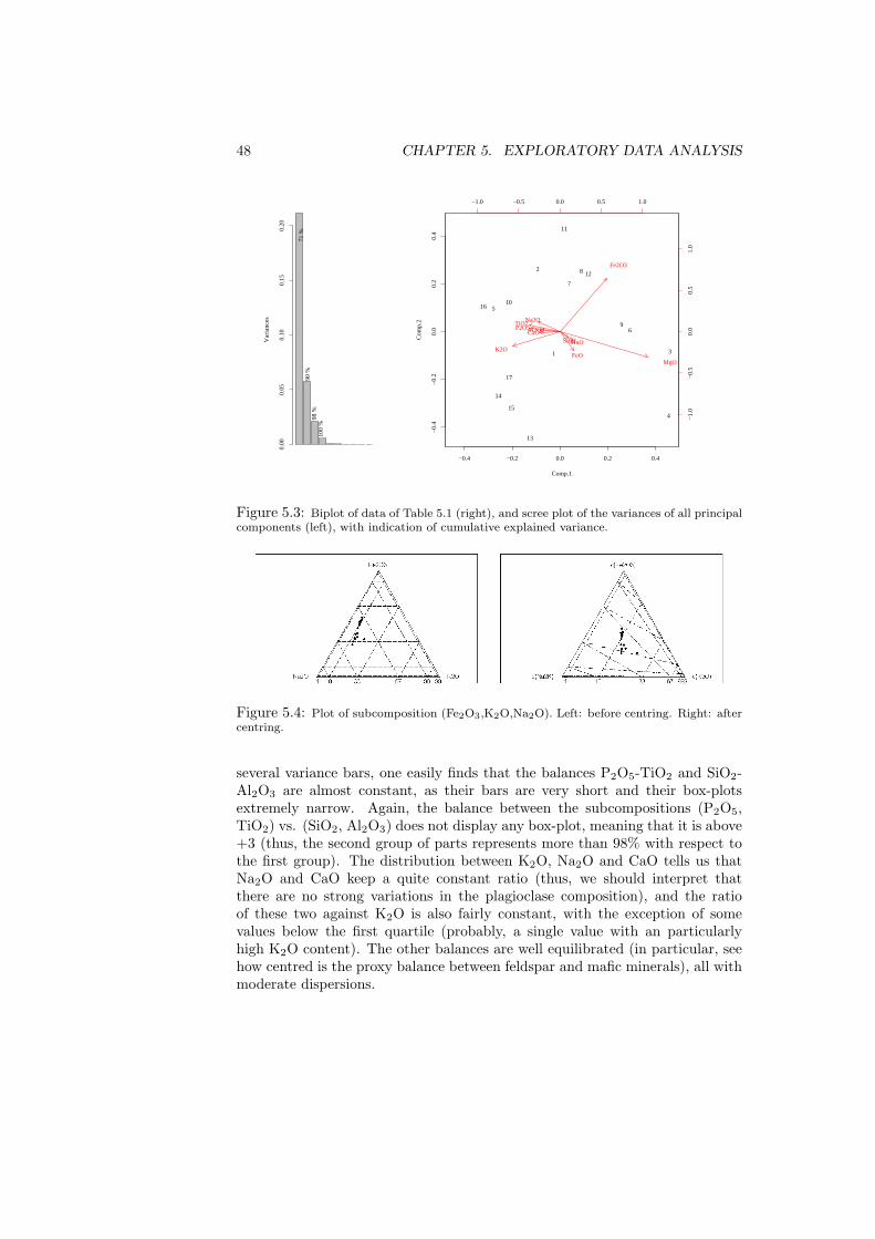
48 CHAPTER 5. EXPLORATORY DATA ANALYSIS
Var
ianc
es
0.00
0.05
0.10
0.15
0.20
71
% 9
0 %
98
%10
0 %
−0.4 −0.2 0.0 0.2 0.4
−0.
4−
0.2
0.0
0.2
0.4
Comp.1
Com
p.2
1
2
3
4
5
6
7
8
9
10
11
12
13
14
15
16
17
−1.0 −0.5 0.0 0.5 1.0
−1.
0−
0.5
0.0
0.5
1.0
SiO2
TiO2Al2O3
Fe2O3
FeO
MnO
MgO
CaO
Na2O
K2O
P2O5
Figure 5.3: Biplot of data of Table 5.1 (right), and scree plot of the variances of all principalcomponents (left), with indication of cumulative explained variance.
Figure 5.4: Plot of subcomposition (Fe2O3,K2O,Na2O). Left: before centring. Right: aftercentring.
several variance bars, one easily finds that the balances P2O5-TiO2 and SiO2-Al2O3 are almost constant, as their bars are very short and their box-plotsextremely narrow. Again, the balance between the subcompositions (P2O5,TiO2) vs. (SiO2, Al2O3) does not display any box-plot, meaning that it is above+3 (thus, the second group of parts represents more than 98% with respect tothe first group). The distribution between K2O, Na2O and CaO tells us thatNa2O and CaO keep a quite constant ratio (thus, we should interpret thatthere are no strong variations in the plagioclase composition), and the ratioof these two against K2O is also fairly constant, with the exception of somevalues below the first quartile (probably, a single value with an particularlyhigh K2O content). The other balances are well equilibrated (in particular, seehow centred is the proxy balance between feldspar and mafic minerals), all withmoderate dispersions.
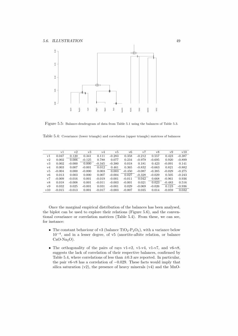
5.6. ILLUSTRATION 49
0.00
0.05
0.10
0.15
0.20
K2O
Na2
O
CaO
MgO
MnO FeO
Fe2O
3
P2O
5
TiO
2
Al2
O3
SiO
2
Figure 5.5: Balance-dendrogram of data from Table 5.1 using the balances of Table 5.3.
Table 5.4: Covariance (lower triangle) and correlation (upper triangle) matrices of balances
v1 v2 v3 v4 v5 v6 v7 v8 v9 v10v1 0.047 0.120 0.341 0.111 -0.283 0.358 -0.212 0.557 0.423 -0.387v2 0.002 0.006 -0.125 0.788 0.077 0.234 -0.979 -0.695 0.920 -0.899v3 0.002 -0.000 0.000 -0.345 -0.380 0.018 0.181 0.423 -0.091 0.141v4 0.003 0.007 -0.001 0.012 0.461 0.365 -0.832 -0.663 0.821 -0.882v5 -0.004 0.000 -0.000 0.003 0.003 -0.450 -0.087 -0.385 -0.029 -0.275v6 0.013 0.003 0.000 0.007 -0.004 0.027 -0.328 -0.029 0.505 -0.243v7 -0.009 -0.016 0.001 -0.019 -0.001 -0.011 0.042 0.668 -0.961 0.936v8 0.018 -0.008 0.001 -0.011 -0.003 -0.001 0.021 0.023 -0.483 0.516v9 0.032 0.025 -0.001 0.031 -0.001 0.029 -0.069 -0.026 0.123 -0.936
v10 -0.015 -0.013 0.001 -0.017 -0.003 -0.007 0.035 0.014 -0.059 0.032
Once the marginal empirical distribution of the balances has been analysed,the biplot can be used to explore their relations (Figure 5.6), and the conven-tional covariance or correlation matrices (Table 5.4). From these, we can see,for instance:
• The constant behaviour of v3 (balance TiO2-P2O5), with a variance below10−4, and in a lesser degree, of v5 (anortite-albite relation, or balanceCaO-Na2O).
• The orthogonality of the pairs of rays v1-v2, v1-v4, v1-v7, and v6-v8,suggests the lack of correlation of their respective balances, confirmed byTable 5.4, where correlations of less than ±0.3 are reported. In particular,the pair v6-v8 has a correlation of −0.029. These facts would imply thatsilica saturation (v2), the presence of heavy minerals (v4) and the MnO-
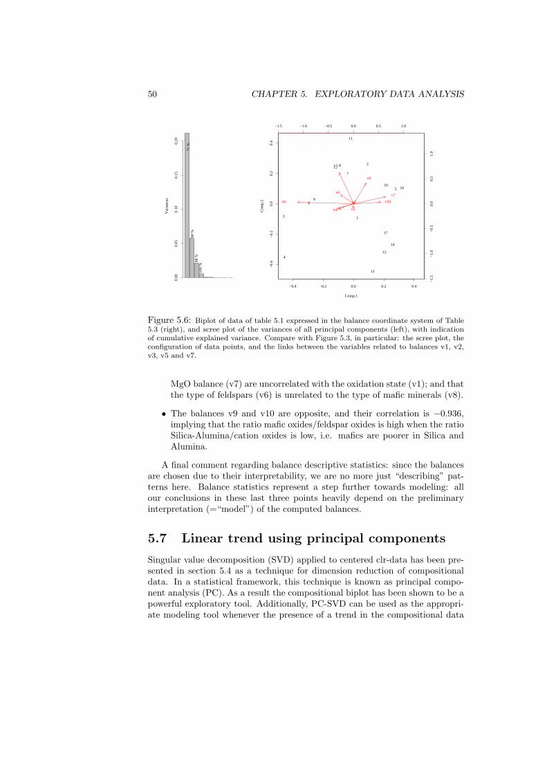
50 CHAPTER 5. EXPLORATORY DATA ANALYSIS
Var
ianc
es
0.00
0.05
0.10
0.15
0.20
71
% 9
0 %
98
%10
0 %
−0.4 −0.2 0.0 0.2 0.4
−0.
4−
0.2
0.0
0.2
0.4
Comp.1
Com
p.2
1
2
3
4
5
6
7
8
9
10
11
12
13
14
15
16
17
−1.5 −1.0 −0.5 0.0 0.5 1.0
−1.
5−
1.0
−0.
50.
00.
51.
0
v1
v2
v3
v4 v5
v6v7
v8
v9 v10
Figure 5.6: Biplot of data of table 5.1 expressed in the balance coordinate system of Table5.3 (right), and scree plot of the variances of all principal components (left), with indicationof cumulative explained variance. Compare with Figure 5.3, in particular: the scree plot, theconfiguration of data points, and the links between the variables related to balances v1, v2,v3, v5 and v7.
MgO balance (v7) are uncorrelated with the oxidation state (v1); and thatthe type of feldspars (v6) is unrelated to the type of mafic minerals (v8).
• The balances v9 and v10 are opposite, and their correlation is −0.936,implying that the ratio mafic oxides/feldspar oxides is high when the ratioSilica-Alumina/cation oxides is low, i.e. mafics are poorer in Silica andAlumina.
A final comment regarding balance descriptive statistics: since the balancesare chosen due to their interpretability, we are no more just “describing” pat-terns here. Balance statistics represent a step further towards modeling: allour conclusions in these last three points heavily depend on the preliminaryinterpretation (=“model”) of the computed balances.
5.7 Linear trend using principal components
Singular value decomposition (SVD) applied to centered clr-data has been pre-sented in section 5.4 as a technique for dimension reduction of compositionaldata. In a statistical framework, this technique is known as principal compo-nent analysis (PC). As a result the compositional biplot has been shown to be apowerful exploratory tool. Additionally, PC-SVD can be used as the appropri-ate modeling tool whenever the presence of a trend in the compositional data
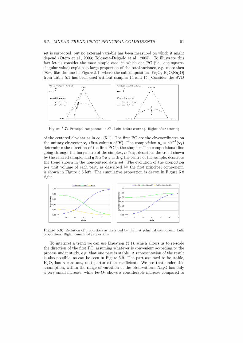
5.7. LINEAR TREND USING PRINCIPAL COMPONENTS 51
set is suspected, but no external variable has been measured on which it mightdepend (Otero et al., 2003; Tolosana-Delgado et al., 2005). To illustrate thisfact let us consider the most simple case, in which one PC (i.e. one square-singular value) explains a large proportion of the total variance, e.g. more then98%, like the one in Figure 5.7, where the subcomposition [Fe2O3,K2O,Na2O]from Table 5.1 has been used without samples 14 and 15. Consider the SVD
Figure 5.7: Principal components in S3. Left: before centring. Right: after centring
of the centered clr-data as in eq. (5.1). The first PC are the clr-coordinates onthe unitary clr-vector v1 (first column of V). The composition a1 = clr−1(v1)determines the direction of the first PC in the simplex. The compositional linegoing through the barycentre of the simplex, α¯ a1, describes the trend shownby the centred sample, and g⊕α¯a1, with g the centre of the sample, describesthe trend shown in the non-centred data set. The evolution of the proportionper unit volume of each part, as described by the first principal component,is shown in Figure 5.8 left. The cumulative proportion is drawn in Figure 5.8right.
0,00
0,20
0,40
0,60
0,80
1,00
-3 -2 -1 0 1 2 3
alpha
pro
po
rcio
nes
Fe2O3 Na2O K2O
0,00
0,20
0,40
0,60
0,80
1,00
1,20
-3 -2 -1 0 1 2 3
alpha
cu
mu
late
d p
rop
ort
ion
s
Fe2O3 Fe2O3+Na2O Fe2O3+Na2O+K2O
Figure 5.8: Evolution of proportions as described by the first principal component. Left:proportions. Right: cumulated proportions.
To interpret a trend we can use Equation (3.1), which allows us to re-scalethe direction of the first PC, assuming whatever is convenient according to theprocess under study, e.g. that one part is stable. A representation of the resultis also possible, as can be seen in Figure 5.9. The part assumed to be stable,K2O, has a constant, unit perturbation coefficient. We see that under thisassumption, within the range of variation of the observations, Na2O has onlya very small increase, while Fe2O3 shows a considerable increase compared to
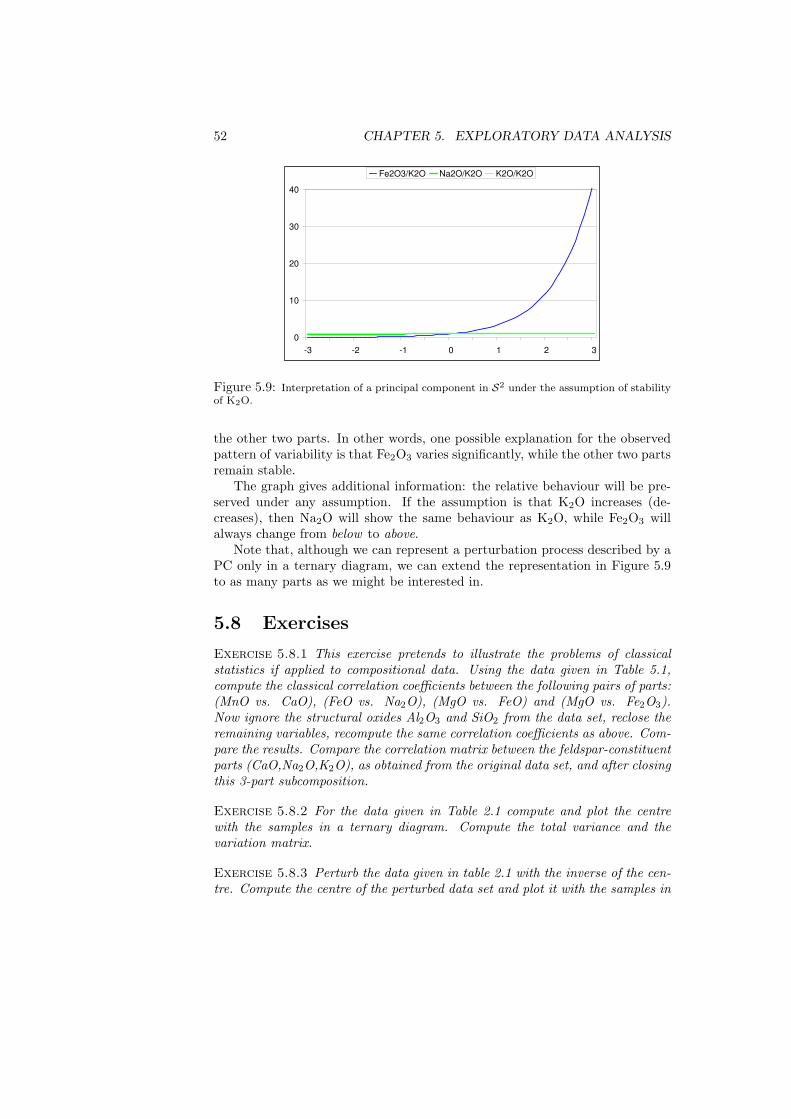
52 CHAPTER 5. EXPLORATORY DATA ANALYSIS
0
10
20
30
40
-3 -2 -1 0 1 2 3
Fe2O3/K2O Na2O/K2O K2O/K2O
Figure 5.9: Interpretation of a principal component in S2 under the assumption of stabilityof K2O.
the other two parts. In other words, one possible explanation for the observedpattern of variability is that Fe2O3 varies significantly, while the other two partsremain stable.
The graph gives additional information: the relative behaviour will be pre-served under any assumption. If the assumption is that K2O increases (de-creases), then Na2O will show the same behaviour as K2O, while Fe2O3 willalways change from below to above.
Note that, although we can represent a perturbation process described by aPC only in a ternary diagram, we can extend the representation in Figure 5.9to as many parts as we might be interested in.
5.8 Exercises
Exercise 5.8.1 This exercise pretends to illustrate the problems of classicalstatistics if applied to compositional data. Using the data given in Table 5.1,compute the classical correlation coefficients between the following pairs of parts:(MnO vs. CaO), (FeO vs. Na2O), (MgO vs. FeO) and (MgO vs. Fe2O3).Now ignore the structural oxides Al2O3 and SiO2 from the data set, reclose theremaining variables, recompute the same correlation coefficients as above. Com-pare the results. Compare the correlation matrix between the feldspar-constituentparts (CaO,Na2O,K2O), as obtained from the original data set, and after closingthis 3-part subcomposition.
Exercise 5.8.2 For the data given in Table 2.1 compute and plot the centrewith the samples in a ternary diagram. Compute the total variance and thevariation matrix.
Exercise 5.8.3 Perturb the data given in table 2.1 with the inverse of the cen-tre. Compute the centre of the perturbed data set and plot it with the samples in
5.8. EXERCISES 53
a ternary diagram. Compute the total variance and the variation matrix. Com-pare your results numerically and graphically with those obtained in exercise5.8.2.
Exercise 5.8.4 Make a biplot of the data given in Table 2.1 and give an inter-pretation.
Exercise 5.8.5 Figure 5.3 shows the biplot of the data given in Table 5.1. Howwould you interpret the different patterns that can be observed?
Exercise 5.8.6 Select 3-part subcompositions that behave in a particular wayin Figure 5.3 and plot them in a ternary diagram. Do they reproduce propertiesmentioned in the previous description?
Exercise 5.8.7 Do a scatter plot of the log-ratios
1√2
lnK2OMgO
against1√2
lnFe2O3
FeO,
identifying each point. Compare with the biplot. Compute the total variance ofthe subcomposition (K2O,MgO,Fe2O3,FeO) and compare it with the total vari-ance of the full data set.
Exercise 5.8.8 How would you recast the data in table 5.1 from mass propor-tion of oxides (as they are) to molar proportions? You may need the followingmolar weights. Any idea of how to do that with a perturbation?
SiO2 TiO2 Al2O3 Fe2O3 FeO MnO60.085 79.899 101.961 159.692 71.846 70.937
MgO CaO Na2O K2O P2O5
40.304 56.079 61.979 94.195 141.945
Exercise 5.8.9 Re-do all the descriptive analysis (and the related exercises)with the Kilauea data set expressed in molar proportions. Compare the results.
Exercise 5.8.10 Compute the vector of arithmetic means of the ilr transformeddata from table 2.1. Apply the ilr−1 backtransformation and compare it with thecentre.
Exercise 5.8.11 Take the parts of the compositions in table 2.1 in a differentorder. Compute the vector of arithmetic means of the ilr transformed sample.Apply the ilr−1 backtransformation. Compare the result with the previous one.
Exercise 5.8.12 Centre the data set of table 2.1. Compute the vector of arith-metic means of the ilr transformed data. What do you obtain?
Exercise 5.8.13 Compute the covariance matrix of the ilr transformed data setof table 2.1 before and after perturbation with the inverse of the centre. Compareboth matrices.

54 CHAPTER 5. EXPLORATORY DATA ANALYSIS
Chapter 6
Distributions on thesimplex
The usual way to pursue any statistical analysis after an exhaustive exploratoryanalysis consists in assuming and testing distributional assumptions for therandom phenomena. This can be easily done for compositional data, as thelinear vector space structure of the simplex allows us to express observationswith respect to an orthonormal basis, a property that guarantees the properapplication of standard statistical methods. The only thing that has to be doneis to perform any standard analysis on orthonormal coefficients and to interpretthe results in terms of coefficients of the orthonormal basis. Once obtained, theinverse can be used to get the same results in terms of the canonical basis ofRD (i.e. as compositions summing up to a constant value). The justificationof this approach lies in the fact that standard mathematical statistics relies onreal analysis, and real analysis is performed on the coefficients with respect toan orthonormal basis in a linear vector space, as discussed by Pawlowsky-Glahn(2003).
There are other ways to justify this approach coming from the side of measuretheory and the definition of density function as the Radon-Nikodym derivativeof a probability measure (Eaton, 1983), but they would divert us too far frompractical applications.
Given that most multivariate techniques rely on the assumption of multi-variate normality, we will concentrate on the expression of this distribution inthe context of random compositions and address briefly other possibilities.
6.1 The normal distribution on SD
Definition 6.1.1 Given a random vector x which sample space is SD, we saythat x follows a normal distribution on SD if, and only if, the vector of or-thonormal coordinates, x∗ = h(x), follows a multivariate normal distributionon RD−1.
55
56 CHAPTER 6. DISTRIBUTIONS ON THE SIMPLEX
To characterise a multivariate normal distribution we need to know its pa-rameters, i.e. the vector of expected values µ and the covariance matrix Σ. Inpractice, they are seldom, if ever, known, and have to be estimated from thesample. Here the maximum likelihood estimates will be used, which are thevector of arithmetic means x∗ for the vector of expected values, and the samplecovariance matrix Sx∗ with the sample size n as divisor. Remember that, in thecase of compositional data, the estimates are computed using the orthonormalcoordinates x∗ of the data and not the original measurements.
As we have considered coordinates x∗, we will obtain results in terms ofcoefficients of x∗ coordinates. To obtain them in terms of the canonical basisof RD we have to backtransform whatever we compute by using the inversetransformation h−1(x∗). In particular, we can backtransform the arithmeticmean x∗, which is an adequate measure of central tendency for data whichfollow reasonably well a multivariate normal distribution. But h−1(x∗) = g,the centre of a compositional data set introduced in Definition 5.2.1, which isan unbiased, minimum variance estimator of the expected value of a randomcomposition (Pawlowsky-Glahn and Egozcue, 2002). Also, as stated in Aitchison(2002), g is an estimate of C [exp(E[ln(x)])], which is the theoretical definitionof the closed geometric mean, thus justifying its use.
6.2 Other distributions
Many other distributions on the simplex have been defined (using on SD theclassical Lebesgue measure on RD), like e.g. the additive logistic skew normal,the Dirichlet and its extensions, the multivariate normal based on Box-Coxtransformations, among others. Some of them have been recently analysed withrespect to the linear vector space structure of the simplex (Mateu-Figueras,2003). This structure has important implications, as the expression of the cor-responding density differs from standard formulae when expressed in terms ofthe metric of the simplex and its associated Lebesgue measure (Pawlowsky-Glahn, 2003). As a result, appealing invariance properties appear: for instance,a normal density on the real line does not change its shape by translation, andthus a normal density in the simplex is also invariant under perturbation; thisproperty is not obtained if one works with the classical Lebesgue measure onRD. These densities and the associated properties shall be addressed in futureextensions of this short course.
6.3 Tests of normality on SD
Testing distributional assumptions of normality on SD is equivalent to testmultivariate normality of h transformed compositions. Thus, interest lies in thefollowing test of hypothesis:
H0: the sample comes from a normal distribution on SD,
6.3. TESTS OF NORMALITY ON SD 57
H1: the sample comes not from a normal distribution on SD,
which is equivalent to
H0: the sample of h coordinates comes from a multivariate normal distribution,
H1: the sample of h coordinates comes not from a multivariate normal distri-bution.
Out of the large number of published tests, for x∗ ∈ RD−1, Aitchison se-lected the Anderson-Darling, Cramer-von Mises, and Watson forms for testinghypothesis on samples coming from a uniform distribution. We repeat themhere for the sake of completeness, but only in a synthetic form. For clarity wefollow the approach used by Pawlowsky-Glahn and Buccianti (2002) and presenteach case separately; in Aitchison (1986) an integrated approach can be found,in which the orthonormal basis selected for the analysis comes from the singularvalue decomposition of the data set.
The idea behind the approach is to compute statistics which under the initialhypothesis should follow a uniform distribution in each of the following threecases:
1. all (D − 1) marginal, univariate distributions,
2. all 12 (D − 1)(D − 2) bivariate angle distributions,
3. the (D − 1)-dimensional radius distribution,
and then use mentioned tests.Another approach is implemented in the R “compositions” library (?), where
all pair-wise log-ratios are checked for normality, in the fashion of the variationmatrix. This gives 1
2 (D − 1)(D − 2) tests of univariate normality: for thehypothesis H0 to hold, all marginal distributions must be also normal. Thiscondition is thus necessary, but not sufficient (although it is a good indication).Here we will not explain the details of this approach: they are equivalent tomarginal univariate distribution tests.
6.3.1 Marginal univariate distributions
We are interested in the distribution of each one of the components of h(x) =x∗ ∈ RD−1, called the marginal distributions. For the i-th of those variables,the observations are given by 〈x, ei〉a, which explicit expression can be found inEquation 4.7. To perform mentioned tests, proceed as follows:
1. Compute the maximum likelihood estimates of the expected value and thevariance:
µi =1n
n∑r=1
x∗ri, σ2i =
1n
n∑r=1
(x∗ri − µi)2.
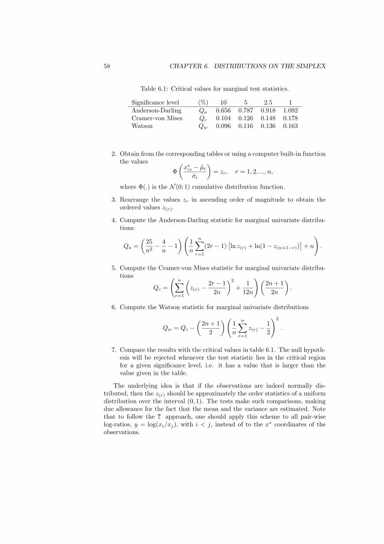
58 CHAPTER 6. DISTRIBUTIONS ON THE SIMPLEX
Table 6.1: Critical values for marginal test statistics.
Significance level (%) 10 5 2.5 1Anderson-Darling Qa 0.656 0.787 0.918 1.092Cramer-von Mises Qc 0.104 0.126 0.148 0.178Watson Qw 0.096 0.116 0.136 0.163
2. Obtain from the corresponding tables or using a computer built-in functionthe values
Φ(
x∗ri − µi
σi
)= zr, r = 1, 2, ..., n,
where Φ(.) is the N (0; 1) cumulative distribution function.
3. Rearrange the values zr in ascending order of magnitude to obtain theordered values z(r).
4. Compute the Anderson-Darling statistic for marginal univariate distribu-tions:
Qa =(
25n2− 4
n− 1
) (1n
n∑r=1
(2r − 1)[ln z(r) + ln(1− z(n+1−r))
]+ n
).
5. Compute the Cramer-von Mises statistic for marginal univariate distribu-tions
Qc =
(n∑
r=1
(z(r) −
2r − 12n
)2
+1
12n
)(2n + 1
2n
).
6. Compute the Watson statistic for marginal univariate distributions
Qw = Qc −(
2n + 12
) (1n
n∑r=1
z(r) −12
)2
.
7. Compare the results with the critical values in table 6.1. The null hypoth-esis will be rejected whenever the test statistic lies in the critical regionfor a given significance level, i.e. it has a value that is larger than thevalue given in the table.
The underlying idea is that if the observations are indeed normally dis-tributed, then the z(r) should be approximately the order statistics of a uniformdistribution over the interval (0, 1). The tests make such comparisons, makingdue allowance for the fact that the mean and the variance are estimated. Notethat to follow the ? approach, one should apply this scheme to all pair-wiselog-ratios, y = log(xi/xj), with i < j, instead of to the x∗ coordinates of theobservations.
6.3. TESTS OF NORMALITY ON SD 59
A visual representation of each test can be given in the form of a plot in theunit square of the z(r) against the associated order statistic (2r − 1)/(2n), r =1, 2, ..., n, of the uniform distribution (a PP plot). Conformity with normalityon SD corresponds to a pattern of points along the diagonal of the square.
6.3.2 Bivariate angle distribution
The next step consists in analysing the bivariate behaviour of the ilr coordi-nates. For each pair of indices (i, j), with i < j, we can form a set of bivariateobservations (x∗ri, x
∗rj), r = 1, 2, ..., n. The test approach here is based on the
following idea: if (ui, uj) is distributed as N 2(0; I2), called a circular normaldistribution, then the radian angle between the vector from (0, 0) to (ui, uj)and the u1-axis is distributed uniformly over the interval (0, 2π). Since any bi-variate normal distribution can be reduced to a circular normal distribution bya suitable transformation, we can apply such a transformation to the bivariateobservations and ask if the hypothesis of the resulting angles following a uniformdistribution can be accepted. Proceed as follows:
1. For each pair of indices (i, j), with i < j, compute the maximum likelihoodestimates
(µi
µj
)=
1n
n∑r=1
x∗ri
1n
n∑r=1
x∗rj
,
(σ2
i σij
σij σ2j
)=
1n
n∑r=1
(x∗ri − x∗i )2 1
n
n∑r=1
(x∗ri − x∗i )(x∗rj − x∗j )
1n
n∑r=1
(x∗ri − x∗i )(x∗rj − x∗j )
1n
n∑r=1
(x∗rj − x∗j )2
.
2. Compute, for r = 1, 2, ..., n,
ur =1√
σ2i σ2
j − σ2ij
[(x∗ri − µi)σj − (x∗rj − µj)
σij
σj
],
vr = (x∗rj − µj)/σj .
3. Compute the radian angles θr required to rotate the ur-axis anticlockwiseabout the origin to reach the points (ur, vr). If arctan(t) denotes the anglebetween − 1
2π and 12π whose tangent is t, then
θr = arctan(
vr
ur+
(1− sgn(ur))π
2+
(1 + sgn(ur)) (1− sgn(vr)) π
4
).
4. Rearrange the values of θr/(2π) in ascending order of magnitude to obtainthe ordered values z(r).
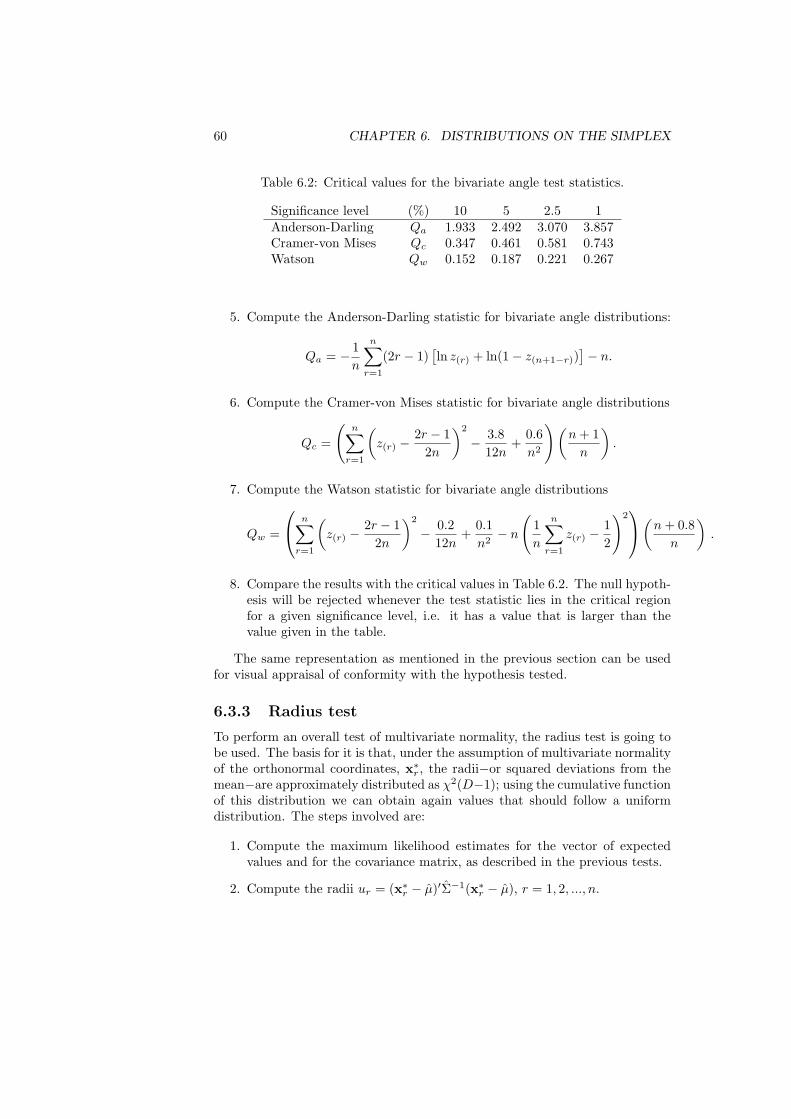
60 CHAPTER 6. DISTRIBUTIONS ON THE SIMPLEX
Table 6.2: Critical values for the bivariate angle test statistics.
Significance level (%) 10 5 2.5 1Anderson-Darling Qa 1.933 2.492 3.070 3.857Cramer-von Mises Qc 0.347 0.461 0.581 0.743Watson Qw 0.152 0.187 0.221 0.267
5. Compute the Anderson-Darling statistic for bivariate angle distributions:
Qa = − 1n
n∑r=1
(2r − 1)[ln z(r) + ln(1− z(n+1−r))
]− n.
6. Compute the Cramer-von Mises statistic for bivariate angle distributions
Qc =
(n∑
r=1
(z(r) −
2r − 12n
)2
− 3.812n
+0.6n2
) (n + 1
n
).
7. Compute the Watson statistic for bivariate angle distributions
Qw =
n∑r=1
(z(r) −
2r − 12n
)2
− 0.212n
+0.1n2
− n
(1n
n∑r=1
z(r) −12
)2
(n + 0.8
n
).
8. Compare the results with the critical values in Table 6.2. The null hypoth-esis will be rejected whenever the test statistic lies in the critical regionfor a given significance level, i.e. it has a value that is larger than thevalue given in the table.
The same representation as mentioned in the previous section can be usedfor visual appraisal of conformity with the hypothesis tested.
6.3.3 Radius test
To perform an overall test of multivariate normality, the radius test is going tobe used. The basis for it is that, under the assumption of multivariate normalityof the orthonormal coordinates, x∗r , the radii−or squared deviations from themean−are approximately distributed as χ2(D−1); using the cumulative functionof this distribution we can obtain again values that should follow a uniformdistribution. The steps involved are:
1. Compute the maximum likelihood estimates for the vector of expectedvalues and for the covariance matrix, as described in the previous tests.
2. Compute the radii ur = (x∗r − µ)′Σ−1(x∗r − µ), r = 1, 2, ..., n.
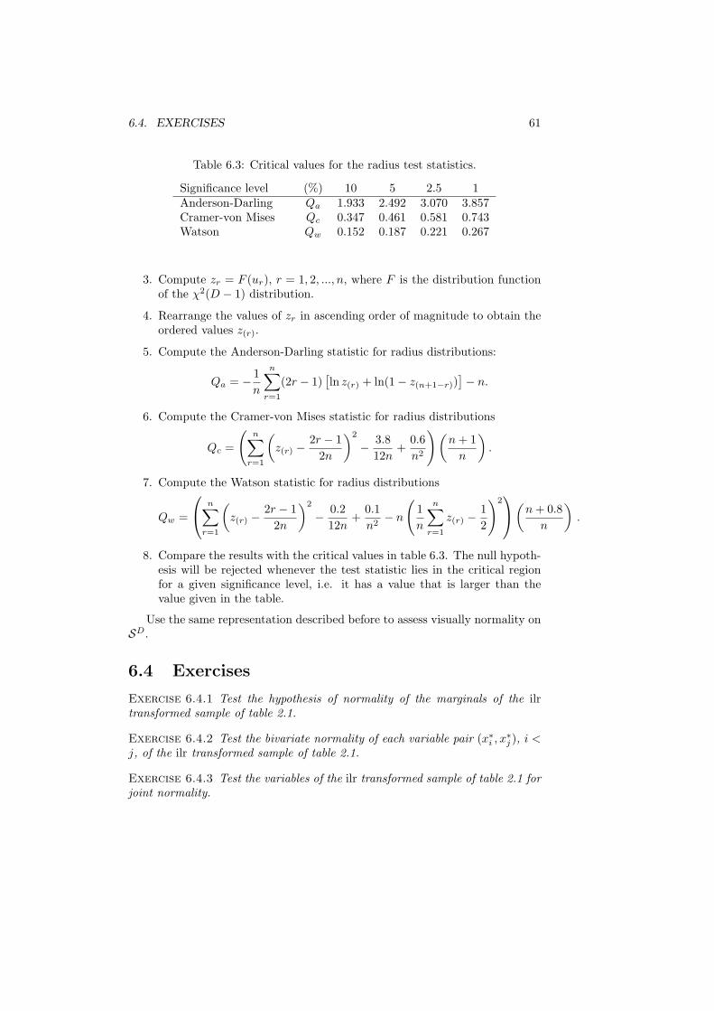
6.4. EXERCISES 61
Table 6.3: Critical values for the radius test statistics.
Significance level (%) 10 5 2.5 1Anderson-Darling Qa 1.933 2.492 3.070 3.857Cramer-von Mises Qc 0.347 0.461 0.581 0.743Watson Qw 0.152 0.187 0.221 0.267
3. Compute zr = F (ur), r = 1, 2, ..., n, where F is the distribution functionof the χ2(D − 1) distribution.
4. Rearrange the values of zr in ascending order of magnitude to obtain theordered values z(r).
5. Compute the Anderson-Darling statistic for radius distributions:
Qa = − 1n
n∑r=1
(2r − 1)[ln z(r) + ln(1− z(n+1−r))
]− n.
6. Compute the Cramer-von Mises statistic for radius distributions
Qc =
(n∑
r=1
(z(r) −
2r − 12n
)2
− 3.812n
+0.6n2
)(n + 1
n
).
7. Compute the Watson statistic for radius distributions
Qw =
n∑r=1
(z(r) −
2r − 12n
)2
− 0.212n
+0.1n2
− n
(1n
n∑r=1
z(r) −12
)2
(n + 0.8
n
).
8. Compare the results with the critical values in table 6.3. The null hypoth-esis will be rejected whenever the test statistic lies in the critical regionfor a given significance level, i.e. it has a value that is larger than thevalue given in the table.
Use the same representation described before to assess visually normality onSD.
6.4 Exercises
Exercise 6.4.1 Test the hypothesis of normality of the marginals of the ilrtransformed sample of table 2.1.
Exercise 6.4.2 Test the bivariate normality of each variable pair (x∗i , x∗j ), i <
j, of the ilr transformed sample of table 2.1.
Exercise 6.4.3 Test the variables of the ilr transformed sample of table 2.1 forjoint normality.

62 CHAPTER 6. DISTRIBUTIONS ON THE SIMPLEX
Chapter 7
Statistical inference
7.1 Testing hypothesis about two groups
When a sample has been divided into two or more groups, interest may liein finding out whether there is a real difference between those groups and, ifit is the case, whether it is due to differences in the centre, in the covariancestructure, or in both. Consider for simplicity two samples of size n1 and n2,which are realisation of two random compositions x1 and x2, each with annormal distribution on the simplex. Consider the following hypothesis:
1. there is no difference between both groups;
2. the covariance structure is the same, but centres are different;
3. the centres are the same, but the covariance structure is different;
4. the groups differ in their centres and in their covariance structure.
Note that if we accept the first hypothesis, it makes no sense to test the second orthe third; the same happens for the second with respect to the third, althoughthese two are exchangeable. This can be considered as a lattice structure inwhich we go from the bottom or lowest level to the top or highest level until weaccept one hypothesis. At that point it makes no sense to test further hypothesisand it is advisable to stop.
To perform tests on these hypothesis, we are going to use coordinates x∗
and to assume they follow each a multivariate normal distribution. For theparameters of the two multivariate normal distributions, the four hypothesisare expressed, in the same order as above, as follows:
1. the vectors of expected values and the covariance matrices are the same:µ1 = µ2 and Σ1 = Σ2;
2. the covariance matrices are the same, but not the vectors of expectedvalues:µ1 6= µ2 and Σ1 = Σ2;
63
64 CHAPTER 7. STATISTICAL INFERENCE
3. the vectors of expected values are the same, but not the covariance ma-trices:µ1 = µ2 and Σ1 6= Σ2;
4. neither the vectors of expected values, nor the covariance matrices are thesame:µ1 6= µ2 and Σ1 6= Σ2.
The last hypothesis is called the model, and the other hypothesis will be con-fronted with it, to see which one is more plausible. In other words, for each test,the model will be the alternative hypothesis H1.
For each single case we can use either unbiased or maximum likelihood esti-mates of the parameters. Under assumptions of multivariate normality, they areidentical for the expected values and have a different divisor of the covariancematrix (the sample size n in the maximum likelihood approach, and n − 1 inthe unbiased case). Here developments will be presented in terms of maximumlikelihood estimates, as those have been used in the previous chapter. Note thatestimators change under each of the possible hypothesis, so each case will bepresented separately. The following developments are based on Aitchison (1986,p. 153-158) and Krzanowski (1988, p. 323-329), although for a complete theo-retical proof Mardia et al. (1979, section 5.5.3) is recommended. The primarycomputations from the coordinates, h(x1) = x∗1, of the n1 samples in one group,and h(x2) = x∗2, of the n2 samples in the other group, are
1. the separate sample estimates
(a) of the vectors of expected values:
µ1 =1n1
n1∑r=1
x∗1r, µ2 =1n2
n2∑s=1
x∗2s,
(b) of the covariance matrices:
Σ1 =1n1
n1∑r=1
(x∗1r − µ1)(x∗1r − µ1)
′,
Σ2 =1n2
n2∑s=1
(x∗2s − µ2)(x∗2s − µ2)
′,
2. the pooled covariance matrix estimate:
Σp =n1Σ1 + n2Σ2
n1 + n2,
3. the combined sample estimates
µc =n1µ1 + n2µ2
n1 + n2,
Σc = Σp +n1n2(µ1 − µ2)(µ1 − µ2)′
(n1 + n2)2.
7.1. TESTING HYPOTHESIS ABOUT TWO GROUPS 65
To test the different hypothesis, we will use the generalised likelihood ra-tio test, which is based on the following principles: consider the maximisedlikelihood function for data x∗ under the null hypothesis, L0(x∗) and underthe model with no restrictions (case 4), Lm(x∗). The test statistic is thenR(x∗) = Lm(x∗)/L0(x∗), and the larger the value is, the more critical or resis-tant to accept the null hypothesis we shall be. In some cases the exact distri-bution of this cases is known. In those cases where it is not known, we shalluse Wilks asymptotic approximation: under the null hypothesis, which placesc constraints on the parameters, the test statistic Q(x∗) = 2 ln(R(x∗)) is dis-tributed approximately as χ2(c). For the cases to be studied, the approximategeneralised ratio test statistic then takes the form:
Q0m(x∗) = n1 ln
(|Σ10||Σ1m|
)+ n2 ln
(|Σ20||Σ2m|
).
1. Equality of centres and covariance structure: The null hypothesis is thatµ1 = µ2 and Σ1 = Σ2, thus we need the estimates of the common pa-rameters µ = µ1 = µ2 and Σ = Σ1 = Σ2, which are, respectively, µc forµ and Σc for Σ under the null hypothesis, and µi for µi and Σi for Σi,i = 1, 2, under the model, resulting in a test statistic
Q1vs4(x∗) = n1 ln
(|Σc||Σ1|
)+ n2 ln
(|Σc||Σ2|
)∼ χ2
(12D(D − 1)
),
to be compared against the upper percentage points of the χ2(
12D(D − 1)
)distribution.
2. Equality of covariance structure with different centres: The null hypothesisis that µ1 6= µ2 and Σ1 = Σ2, thus we need the estimates of µ1, µ2 andof the common covariance matrix Σ = Σ1 = Σ2, which are Σp for Σ underthe null hypothesis and Σi for Σi, i = 1, 2, under the model, resulting ina test statistic
Q2vs4(x∗) = n1 ln
(|Σp||Σ1|
)+ n2 ln
(|Σp||Σ2|
)∼ χ2
(12(D − 1)(D − 2)
).
3. Equality of centres with different covariance structure: The null hypothesisis that µ1 = µ2 and Σ1 6= Σ2, thus we need the estimates of the commoncentre µ = µ1 = µ2 and of the covariance matrices Σ1 and Σ2. In thiscase no explicit form for the maximum likelihood estimates exists. Hencethe need for a simple iterative method which requires the following steps:
(a) Set the initial value Σih = Σi, i = 1, 2;
(b) compute the common mean, weighted by the variance of each group:
µh = (n1Σ−11h + n2Σ−1
2h )−1(n1Σ−11h µ1 + n2Σ−1
2h µ2) ;
66 CHAPTER 7. STATISTICAL INFERENCE
(c) compute the variances of each group with respect to the commonmean:
Σih = Σi + (µi − µh)(µi − µh)′ , i = 1, 2 ;
(d) Repeat steps 2 and 3 until convergence.
Thus we have Σi0 for Σi, i = 1, 2, under the null hypothesis and Σi forΣi, i = 1, 2, under the model, resulting in a test statistic
Q3vs4(x∗) = n1 ln
(|Σ1h||Σ1|
)+ n2 ln
(|Σ2h||Σ2|
)∼ χ2(D − 1).
7.2 Probability and confidence regions for com-positional data
Like confidence intervals, confidence regions are a measure of variability, al-though in this case it is a measure of joint variability for the variables involved.They can be of interest in themselves, to analyse the precision of the estimationobtained, but more frequently they are used to visualise differences betweengroups. Recall that for compositional data with three components, confidenceregions can be plotted in the corresponding ternary diagram, thus giving ev-idence of the relative behaviour of the various centres, or of the populationsthemselves. The following method to compute confidence regions assumes ei-ther multivariate normality, or the size of the sample to be large enough for themultivariate central limit theorem to hold.
Consider a composition x ∈ SD and assume it follows a normal distributionon SD as defined in section 6.1.1. Then, the (D − 1)-variate vector x∗ = h(x)follows a multivariate normal distribution.
Three different cases might be of interest:
1. we know the true mean vector and the true variance matrix of the randomvector x∗, and want to plot a probability region;
2. we do not know the mean vector and variance matrix of the random vector,and want to plot a confidence region for its mean using a sample of size n,
3. we do not know the mean vector and variance matrix of the random vector,and want to plot a probability region (incorporating our uncertainty).
In the first case, if a random vector x∗ follows a multivariate normal distri-bution with known parameters µ and Σ, then
(x∗ − µ)Σ−1(x∗ − µ)′ ∼ χ2(D − 1),
is a chi square distribution of D − 1 degrees of freedom. Thus, for given α, wemay obtain (through software or tables) a value κ such that
1− α = P[(x∗ − µ)Σ−1(x∗ − µ)′ ≤ κ
]. (7.1)
7.3. EXERCISES 67
This defines a (1 − α)100% probability region centred at µ in RD, and conse-quently x = h−1(x∗) defines a (1 − α)100% probability region centred at themean in the simplex.
Regarding the second case, it is well known that for a sample of size n (andx∗ normally-distributed or n big enough), the maximum likelihood estimates x∗
and Σ satisfy that
n−D + 1D − 1
(x∗ − µ)Σ−1(x∗ − µ)′ ∼ F(D − 1, n−D + 1),
follows a Fisher F distribution on (D − 1, n − D + 1) degrees of freedom(Krzanowski, 1988, see p. 227-228 for further details). Again, for given α,we may obtain a value c such that
1− α = P[n−D + 1
D − 1(x∗ − µ)Σ−1(x∗ − µ)′ ≤ c
]
= P[(x∗ − µ)Σ−1(x∗ − µ)′ ≤ κ
], (7.2)
with κ = D−1n−D+1c. But (x∗ − µ)Σ−1(x∗ − µ)′ = κ (constant) defines a (1 −
α)100% confidence region centred at x∗ in RD, and consequently ξ = h−1(µ)defines a (1− α)100% confidence region around the centre in the simplex.
Finally, in the third case, one should actually use the multivariate Student-Siegel predictive distribution: a new value of x∗ will have as density
f(x∗|data) ∝[1 + (n− 1)
(1− 1
n
)(x∗ − x∗) · Σ
]−1
· [(x∗ − x∗)′]n/2.
This distribution is unfortunately not commonly tabulated, and it is only avail-able in some specific packages. On the other side, if n is large with respect toD, the differences between the first and third options are negligible.
Note that for D = 3, D − 1 = 2 and we have an ellipse in real space, in anyof the first two cases: the only difference between them is how the constant κis computed. The parameterisation equations in polar coordinates, which arenecessary to plot these ellipses, are given in Appendix B.
7.3 Exercises
Exercise 7.3.1 Divide the sample of Table 5.1 into two groups (at your will)and perform the different tests on the centres and covariance structures.
Exercise 7.3.2 Compute and plot a confidence region for the ilr transformedmean of the data from table 2.1 in R2.
Exercise 7.3.3 Transform the confidence region of exercise 7.3.2 back into theternary diagram using ilr−1.

68 CHAPTER 7. STATISTICAL INFERENCE
Exercise 7.3.4 Compute and plot a 90% probability region for the ilr trans-formed data of table 2.1 in R2, together with the sample. Use the chi squaredistribution.
Exercise 7.3.5 For each of the four hypothesis in section 7.1, compute thenumber of parameters to be estimated if the composition has D parts. Thefourth hypothesis needs more parameters than the other three. How many, withrespect to each of the three simpler hypothesis? Compare with the degrees offreedom of the χ2 distributions of page 65.
Chapter 8
Compositional processes
Compositions can evolve depending on an external parameter like space, time,temperature, pressure, global economic conditions and many other ones. Theexternal parameter may be continuous or discrete. In general, the evolution isexpressed as a function x(t), where t represents the external variable and theimage is a composition in SD. In order to model compositional processes, thestudy of simple models appearing in practice is very important. However, ap-parently complicated behaviours represented in ternary diagrams may be closeto linear processes in the simplex. The main challenge is frequently to identifycompositional processes from available data. This is done using a variety oftechniques that depend on the data, the selected model of the process and theprior knowledge about them. Next subsections present three simple examplesof such processes. The most important is the linear process in the simplex, thatfollows a straight-line in the simplex. Other frequent process are the comple-mentary processes and mixtures. In order to identify the models, two standardtechniques are presented: regression and principal component analysis in thesimplex. The first one is adequate when compositional data are completedwith some external covariates. Contrarily, principal component analysis tries toidentify directions of maximum variability of data, i.e. a linear process in thesimplex with some unobserved covariate.
8.1 Linear processes: exponential growth or de-cay of mass
Consider D different species of bacteria which reproduce in a rich medium andassume there are no interaction between the species. It is well-known thatthe mass of each species grows proportionally to the previous mass and thiscauses an exponential growth of the mass of each species. If t is time and eachcomponent of the vector x(t) represents the mass of a species at the time t, themodel is
x(t) = x(0) · exp(λt) , (8.1)
69
70 CHAPTER 8. COMPOSITIONAL PROCESSES
where λ = [λ1, λ2, . . . , λD] contains the rates of growth corresponding to thespecies. In this case, λi will be positive, but one can imagine λi = 0, the i-thspecies does not vary; or λi < 0, the i-th species decreases with time. Model(8.1) represents a process in which both the total mass of bacteria and thecomposition of the mass by species are specified. Normally, interest is centredin the compositional aspect of (8.1) which is readily obtained applying a closureto the equation (8.1). From now on, we assume that x(t) is in SD.
A simple inspection of (8.1) permits to write it using the operations of thesimplex,
x(t) = x(0)⊕ t¯ p , p = exp(λ) , (8.2)
where a straight-line is identified: x(0) is a point on the line taken as the origin;p is a constant vector representing the direction of the line; and t is a parameterwith values on the real line (positive or negative).
The linear character of this process is enhanced when it is represented usingcoordinates. Select a basis in SD, for instance, using balances determined bya sequential binary partition, and denote the coordinates u(t) = ilr(x)(t), q =ilr(p). The model for the coordinates is then
u(t) = u(0) + t · q , (8.3)
a typical expression of a straight-line in RD−1. The processes that follow astraight-line in the simplex are more general than those represented by Equa-tions (8.2) and (8.3), because changing the parameter t by any function φ(t) inthe expression, still produces images on the same straight-line.
Example 8.1.1 (growth of bacteria population) Set D = 3 and con-sider species 1, 2, 3, whose relative masses were 82.7%, 16.5% and 0.8% atthe initial observation (t = 0). The rates of growth are known to be λ1 = 1,λ2 = 2 and λ3 = 3. Select the sequential binary partition and balances specifiedin Table 8.1.
Table 8.1: Sequential binary partition and balance-coordinates used in the example growthof bacteria population
order x1 x2 x3 balance-coord.
1 +1 +1 −1 u1 = 1√6
ln x1x2x23
2 +1 −1 0 u2 = 1√2
ln x1x2
The process of growth is shown in Figure 8.1, both in a ternary diagram(left) and in the plane of the selected coordinates (right). Using coordinates itis easy to identify that the process corresponds to a straight-line in the simplex.Figure 8.2 shows the evolution of the process in time in two usual plots: the oneon the left shows the evolution of each part-component in per unit; on the right,
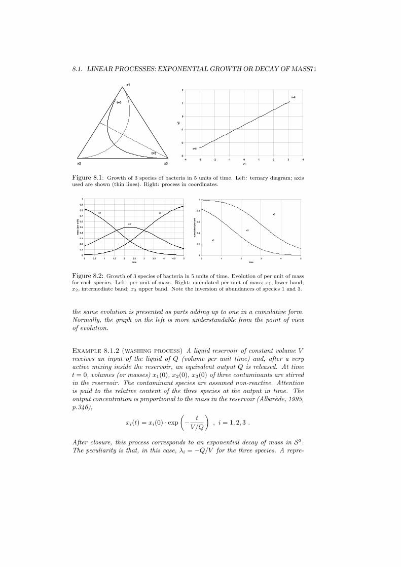
8.1. LINEAR PROCESSES: EXPONENTIAL GROWTH OR DECAY OF MASS71
x1
x2 x3
t=0
t=5-3
-2
-1
0
1
2
-4 -3 -2 -1 0 1 2 3 4
u1
u2
t=0
t=5
Figure 8.1: Growth of 3 species of bacteria in 5 units of time. Left: ternary diagram; axisused are shown (thin lines). Right: process in coordinates.
0
0.1
0.2
0.3
0.4
0.5
0.6
0.7
0.8
0.9
1
0 0.5 1 1.5 2 2.5 3 3.5 4 4.5 5
time
ma
ss
(p
er
un
it)
x1
x2
x3
0
0.2
0.4
0.6
0.8
1
0 1 2 3 4 5
time
cu
mu
late
d p
er
un
it
x1
x2
x3
Figure 8.2: Growth of 3 species of bacteria in 5 units of time. Evolution of per unit of massfor each species. Left: per unit of mass. Right: cumulated per unit of mass; x1, lower band;x2, intermediate band; x3 upper band. Note the inversion of abundances of species 1 and 3.
the same evolution is presented as parts adding up to one in a cumulative form.Normally, the graph on the left is more understandable from the point of viewof evolution.
Example 8.1.2 (washing process) A liquid reservoir of constant volume Vreceives an input of the liquid of Q (volume per unit time) and, after a veryactive mixing inside the reservoir, an equivalent output Q is released. At timet = 0, volumes (or masses) x1(0), x2(0), x3(0) of three contaminants are stirredin the reservoir. The contaminant species are assumed non-reactive. Attentionis paid to the relative content of the three species at the output in time. Theoutput concentration is proportional to the mass in the reservoir (Albarede, 1995,p.346),
xi(t) = xi(0) · exp(− t
V/Q
), i = 1, 2, 3 .
After closure, this process corresponds to an exponential decay of mass in S3.The peculiarity is that, in this case, λi = −Q/V for the three species. A repre-
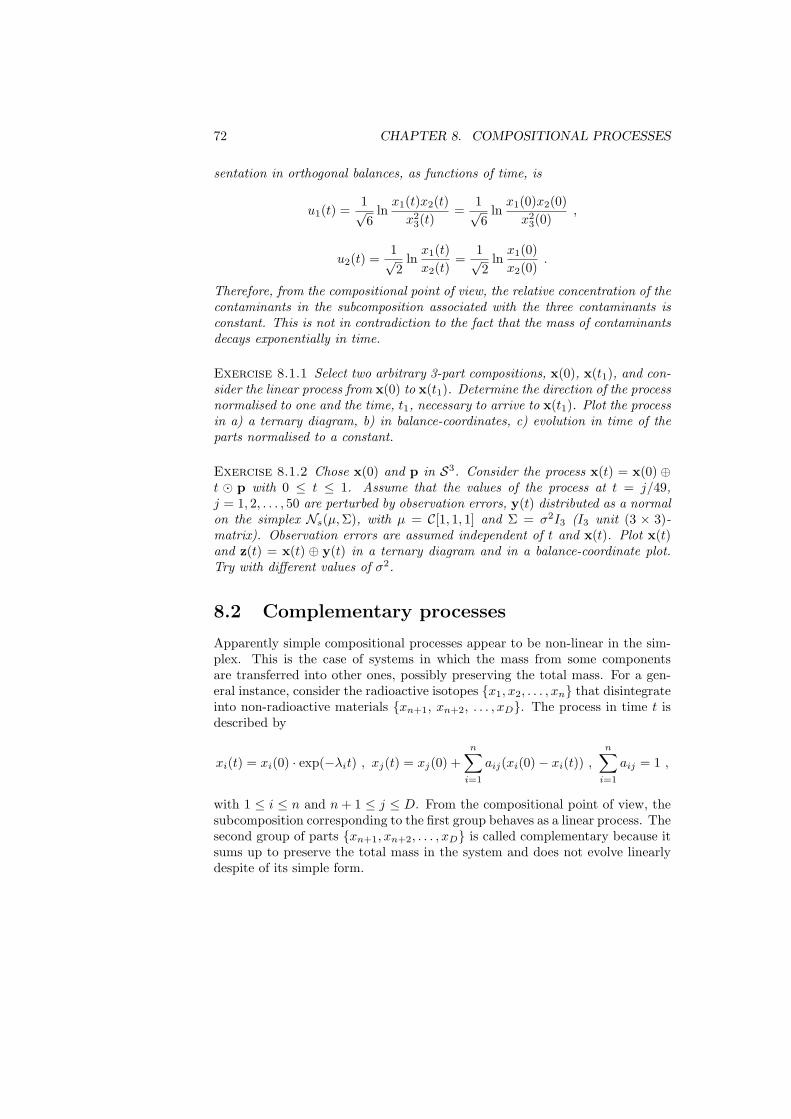
72 CHAPTER 8. COMPOSITIONAL PROCESSES
sentation in orthogonal balances, as functions of time, is
u1(t) =1√6
lnx1(t)x2(t)
x23(t)
=1√6
lnx1(0)x2(0)
x23(0)
,
u2(t) =1√2
lnx1(t)x2(t)
=1√2
lnx1(0)x2(0)
.
Therefore, from the compositional point of view, the relative concentration of thecontaminants in the subcomposition associated with the three contaminants isconstant. This is not in contradiction to the fact that the mass of contaminantsdecays exponentially in time.
Exercise 8.1.1 Select two arbitrary 3-part compositions, x(0), x(t1), and con-sider the linear process from x(0) to x(t1). Determine the direction of the processnormalised to one and the time, t1, necessary to arrive to x(t1). Plot the processin a) a ternary diagram, b) in balance-coordinates, c) evolution in time of theparts normalised to a constant.
Exercise 8.1.2 Chose x(0) and p in S3. Consider the process x(t) = x(0) ⊕t ¯ p with 0 ≤ t ≤ 1. Assume that the values of the process at t = j/49,j = 1, 2, . . . , 50 are perturbed by observation errors, y(t) distributed as a normalon the simplex Ns(µ, Σ), with µ = C[1, 1, 1] and Σ = σ2I3 (I3 unit (3 × 3)-matrix). Observation errors are assumed independent of t and x(t). Plot x(t)and z(t) = x(t) ⊕ y(t) in a ternary diagram and in a balance-coordinate plot.Try with different values of σ2.
8.2 Complementary processes
Apparently simple compositional processes appear to be non-linear in the sim-plex. This is the case of systems in which the mass from some componentsare transferred into other ones, possibly preserving the total mass. For a gen-eral instance, consider the radioactive isotopes {x1, x2, . . . , xn} that disintegrateinto non-radioactive materials {xn+1, xn+2, . . . , xD}. The process in time t isdescribed by
xi(t) = xi(0) · exp(−λit) , xj(t) = xj(0) +n∑
i=1
aij(xi(0)− xi(t)) ,
n∑
i=1
aij = 1 ,
with 1 ≤ i ≤ n and n + 1 ≤ j ≤ D. From the compositional point of view, thesubcomposition corresponding to the first group behaves as a linear process. Thesecond group of parts {xn+1, xn+2, . . . , xD} is called complementary because itsums up to preserve the total mass in the system and does not evolve linearlydespite of its simple form.
8.2. COMPLEMENTARY PROCESSES 73
Example 8.2.1 (one radioactive isotope) Consider the radioactive isotopex1 which is transformed into the non-radioactive isotope x3, while the elementx2 remains unaltered. This situation, with λ1 < 0, corresponds to
x1(t) = x1(0) · exp(λ1t) , x2(t) = x2(0) , x3(t) = x3(0) + x1(0)− x1(t) ,
that is mass preserving. The group of parts behaving linearly is {x1, x2}, anda complementary group is {x3}. Table 8.2 shows parameters of the model andFigures 8.3 and 8.4 show different aspects of the compositional process fromt = 0 to t = 10.
Table 8.2: Parameters for Example 8.2.1: one radioactive isotope. Disintegration rate is ln 2times the inverse of the half-lifetime. Time units are arbitrary. The lower part of the tablerepresents the sequential binary partition used to define the balance-coordinates.
parameter x1 x2 x3
disintegration rate 0.5 0.0 0.0initial mass 1.0 0.4 0.5balance 1 +1 +1 −1balance 2 +1 −1 0
x1
x2 x3
t=0
t=5
-4
-3
-2
-1
0
1
-3 -2.5 -2 -1.5 -1 -0.5 0 0.5
u1
u2
t=0
t=10
Figure 8.3: Disintegration of one isotope x1 into x3 in 10 units of time. Left: ternarydiagram; axis used are shown (thin lines). Right: process in coordinates. The mass in thesystem is constant and the mass of x2 is constant.
A first inspection of the Figures reveals that the process appears as a segmentin the ternary diagram (Fig. 8.3, right). This fact is essentially due to the con-stant mass of x2 in a conservative system, thus appearing as a constant per-unit.In figure 8.3, left, the evolution of the coordinates shows that the process is notlinear; however, except for initial times, the process may be approximated by alinear one. The linear or non-linear character of the process is hardly detectedin Figures 8.4 showing the evolution in time of the composition.
74 CHAPTER 8. COMPOSITIONAL PROCESSES
0
0.1
0.2
0.3
0.4
0.5
0.6
0.7
0.8
0.9
0 1 2 3 4 5 6 7 8 9 10
time
ma
ss
(p
er
un
it)
x1
x2
x3
0
0.2
0.4
0.6
0.8
1
0 1 2 3 4 5 6 7 8 9 10
time
cu
mu
late
d p
er
un
it
x1x2
x3
Figure 8.4: Disintegration of one isotope x1 into x3 in 10 units of time. Evolution of perunit of mass for each species. Left: per unit of mass. Right: cumulated per unit of mass;x1, lower band; x2, intermediate band; x3 upper band. Note the inversion of abundances ofspecies 1 and 3.
Example 8.2.2 (three radioactive isotopes) Consider three radioactive iso-topes that we identify with a linear group of parts, {x1, x2, x3}. The disintegratedmass of x1 is distributed on the non-radioactive parts {x4, x5, x6} (complemen-tary group). The whole disintegrated mass from x2 and x3 is assigned to x4 andx5 respectively. The values of the parameters considered are shown in Table
Table 8.3: Parameters for Example 8.2.2: three radioactive isotopes. Disintegration rate isln 2 times the inverse of the half-lifetime. Time units are arbitrary. The middle part of thetable corresponds to the coefficients aij indicating the part of the mass from xi componenttransformed into the xj . Note they add to one and the system is mass conservative. The lowerpart of the table shows the sequential binary partition to define the balance coordinates.
parameter x1 x2 x3 x4 x5 x6
disintegration rate 0.2 0.04 0.4 0.0 0.0 0.0initial mass 30.0 50.0 13.0 1.0 1.2 0.7
mass from x1 0.0 0.0 0.0 0.7 0.2 0.1mass from x2 0.0 0.0 0.0 0.0 1.0 0.0mass from x3 0.0 0.0 0.0 0.0 0.0 1.0
balance 1 +1 +1 +1 −1 −1 −1balance 2 +1 +1 −1 0 0 0balance 3 +1 −1 0 0 0 0balance 4 0 0 0 +1 +1 −1balance 5 0 0 0 +1 −1 0
8.3. Figure 8.5 (left) shows the evolution of the subcomposition of the comple-mentary group in 20 time units; no special conclusion is got from it. Contrarily,Figure 8.5 (right), showing the evolution of the coordinates of the subcomposi-tion, reveals a loop in the evolution with a double point (the process passes twotimes through this compositional point); although less clearly, the same fact canbe observed in the representation of the ternary diagram in Figure 8.6. This isa quite surprising and involved behaviour despite of the very simple character
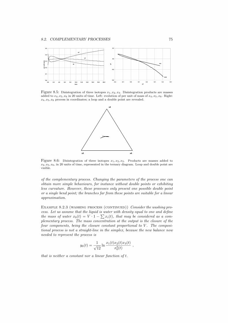
8.2. COMPLEMENTARY PROCESSES 75
0.0
0.1
0.2
0.3
0.4
0.5
0.0 2.0 4.0 6.0 8.0 10.0 12.0 14.0 16.0 18.0 20.0
time
pe
r u
nit
ma
ss
x5
x4
x6
-0.4
-0.2
0.0
0.2
-0.2 -0.1 0.0 0.1 0.2 0.3 0.4 0.5
y4
y5 t=0
t=20
Figure 8.5: Disintegration of three isotopes x1, x2, x3. Disintegration products are massesadded to x4, x5, x6 in 20 units of time. Left: evolution of per unit of mass of x4, x5, x6. Right:x4, x5, x6 process in coordinates; a loop and a double point are revealed.
x4
x5 x6
Figure 8.6: Disintegration of three isotopes x1, x2, x3. Products are masses added tox4, x5, x6, in 20 units of time, represented in the ternary diagram. Loop and double point arevisible.
of the complementary process. Changing the parameters of the process one canobtain more simple behaviours, for instance without double points or exhibitingless curvature. However, these processes only present one possible double pointor a single bend point; the branches far from these points are suitable for a linearapproximation.
Example 8.2.3 (washing process (continued)) Consider the washing pro-cess. Let us assume that the liquid is water with density equal to one and definethe mass of water x0(t) = V · 1 − ∑
xi(t), that may be considered as a com-plementary process. The mass concentration at the output is the closure of thefour components, being the closure constant proportional to V . The composi-tional process is not a straight-line in the simplex, because the new balance nowneeded to represent the process is
y0(t) =1√12
lnx1(t)x2(t)x3(t)
x30(t)
,
that is neither a constant nor a linear function of t.
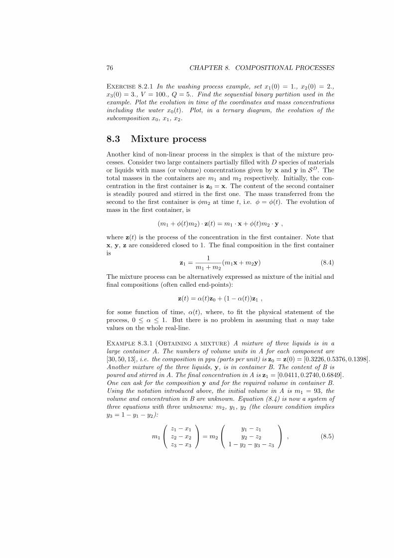
76 CHAPTER 8. COMPOSITIONAL PROCESSES
Exercise 8.2.1 In the washing process example, set x1(0) = 1., x2(0) = 2.,x3(0) = 3., V = 100., Q = 5.. Find the sequential binary partition used in theexample. Plot the evolution in time of the coordinates and mass concentrationsincluding the water x0(t). Plot, in a ternary diagram, the evolution of thesubcomposition x0, x1, x2.
8.3 Mixture process
Another kind of non-linear process in the simplex is that of the mixture pro-cesses. Consider two large containers partially filled with D species of materialsor liquids with mass (or volume) concentrations given by x and y in SD. Thetotal masses in the containers are m1 and m2 respectively. Initially, the con-centration in the first container is z0 = x. The content of the second containeris steadily poured and stirred in the first one. The mass transferred from thesecond to the first container is φm2 at time t, i.e. φ = φ(t). The evolution ofmass in the first container, is
(m1 + φ(t)m2) · z(t) = m1 · x + φ(t)m2 · y ,
where z(t) is the process of the concentration in the first container. Note thatx, y, z are considered closed to 1. The final composition in the first containeris
z1 =1
m1 + m2(m1x + m2y) (8.4)
The mixture process can be alternatively expressed as mixture of the initial andfinal compositions (often called end-points):
z(t) = α(t)z0 + (1− α(t))z1 ,
for some function of time, α(t), where, to fit the physical statement of theprocess, 0 ≤ α ≤ 1. But there is no problem in assuming that α may takevalues on the whole real-line.
Example 8.3.1 (Obtaining a mixture) A mixture of three liquids is in alarge container A. The numbers of volume units in A for each component are[30, 50, 13], i.e. the composition in ppu (parts per unit) is z0 = z(0) = [0.3226, 0.5376, 0.1398].Another mixture of the three liquids, y, is in container B. The content of B ispoured and stirred in A. The final concentration in A is z1 = [0.0411, 0.2740, 0.6849].One can ask for the composition y and for the required volume in container B.Using the notation introduced above, the initial volume in A is m1 = 93, thevolume and concentration in B are unknown. Equation (8.4) is now a system ofthree equations with three unknowns: m2, y1, y2 (the closure condition impliesy3 = 1− y1 − y2):
m1
z1 − x1
z2 − x2
z3 − x3
= m2
y1 − z1
y2 − z2
1− y2 − y3 − z3
, (8.5)
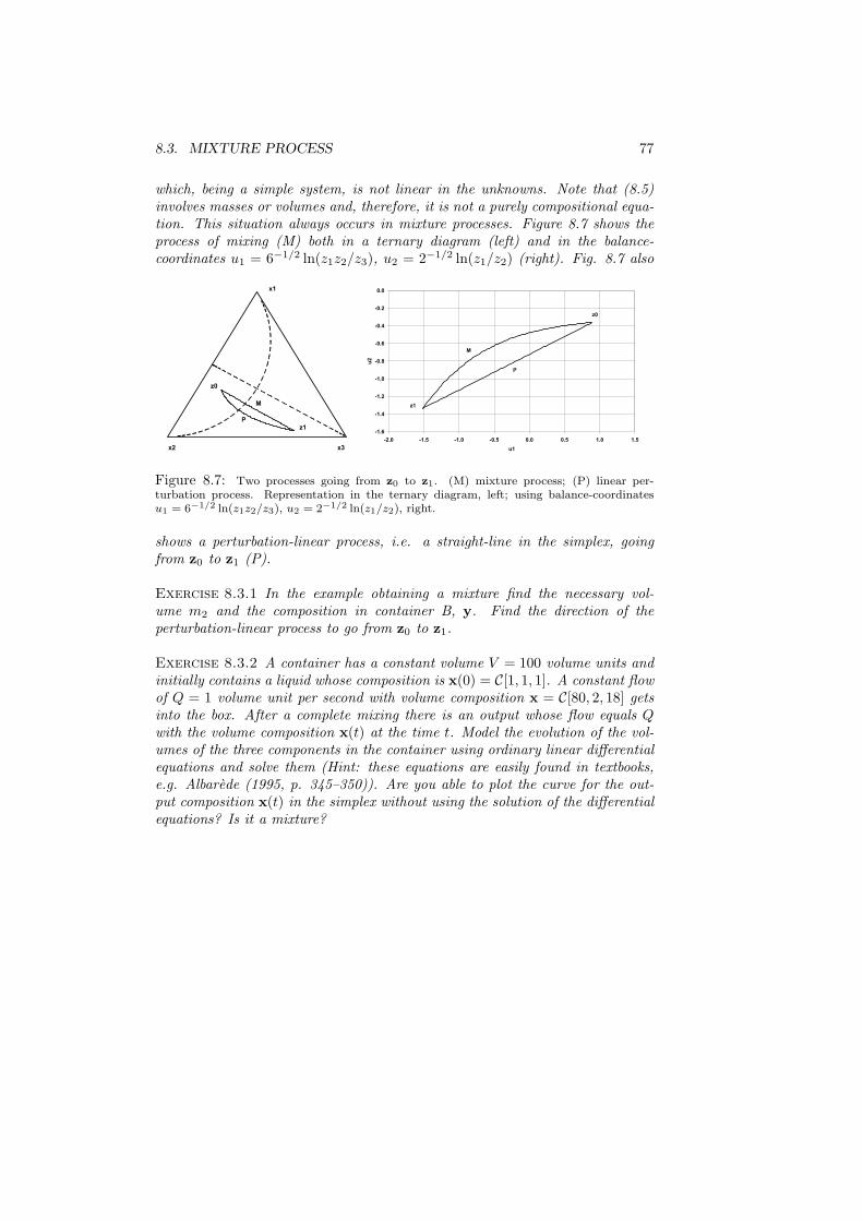
8.3. MIXTURE PROCESS 77
which, being a simple system, is not linear in the unknowns. Note that (8.5)involves masses or volumes and, therefore, it is not a purely compositional equa-tion. This situation always occurs in mixture processes. Figure 8.7 shows theprocess of mixing (M) both in a ternary diagram (left) and in the balance-coordinates u1 = 6−1/2 ln(z1z2/z3), u2 = 2−1/2 ln(z1/z2) (right). Fig. 8.7 also
P
M
x1
x2 x3
z0
z1-1.6
-1.4
-1.2
-1.0
-0.8
-0.6
-0.4
-0.2
0.0
-2.0 -1.5 -1.0 -0.5 0.0 0.5 1.0 1.5
u1
u2
M
P
z0
z1
Figure 8.7: Two processes going from z0 to z1. (M) mixture process; (P) linear per-turbation process. Representation in the ternary diagram, left; using balance-coordinatesu1 = 6−1/2 ln(z1z2/z3), u2 = 2−1/2 ln(z1/z2), right.
shows a perturbation-linear process, i.e. a straight-line in the simplex, goingfrom z0 to z1 (P).
Exercise 8.3.1 In the example obtaining a mixture find the necessary vol-ume m2 and the composition in container B, y. Find the direction of theperturbation-linear process to go from z0 to z1.
Exercise 8.3.2 A container has a constant volume V = 100 volume units andinitially contains a liquid whose composition is x(0) = C[1, 1, 1]. A constant flowof Q = 1 volume unit per second with volume composition x = C[80, 2, 18] getsinto the box. After a complete mixing there is an output whose flow equals Qwith the volume composition x(t) at the time t. Model the evolution of the vol-umes of the three components in the container using ordinary linear differentialequations and solve them (Hint: these equations are easily found in textbooks,e.g. Albarede (1995, p. 345–350)). Are you able to plot the curve for the out-put composition x(t) in the simplex without using the solution of the differentialequations? Is it a mixture?

78 CHAPTER 8. COMPOSITIONAL PROCESSES
Chapter 9
Linear compositionalmodels
Linear models are intended to relate two sets of random variables using linearrelationships. They are very general and appear routinely in many statistical ap-plications. A first set of variables, called response variables, are to be predictedfrom a second set of variables, called predictors or covariates. Linear combi-nations of the predictors, transformed by some non-linear function, frequentlycalled link function, are used to get a predictor function approaching responses.Errors or residuals are measured as Euclidean differences between responses andthe predictor function. There is a extensive literature on general linear models,for instance Anderson (1984). The two sets of variables may have very differ-ent characteristics (categorical, real, discrete) and the link functions choices arealso multiple. We are here interested in cases where responses or predictorshave compositional character. When the response is compositional we mustbe aware that residuals should be measured with compositional distances, i.e.within the framework of Aitchison geometry of the simplex. Section 9.1 treatsthe case where the response is compositional and the covariates are real or dis-crete thus corresponding to a multiple regression. Response is handled using itscoordinates. The ilr transformation plays the role of a link function. Section 9.2assumes a single real response and a compositional predictor. Again ilr plays animportant role. Section 9.3 discusses the case in which the response is composi-tional and the predictors reduce to a categorical variable indicating a treatmentor a subpopulation. The goal of such an analysis of variance (ANOVA) model isto decide whether the center of compositions across the treatments are equal ornot. Section 9.4 deals with discriminant analysis. In this case, response is a cat-egory to which a compositional observation (predictor) is assigned. The modelis then a rule to assign an observed composition to categories or treatments andit provides a probability of belonging for each category.
79
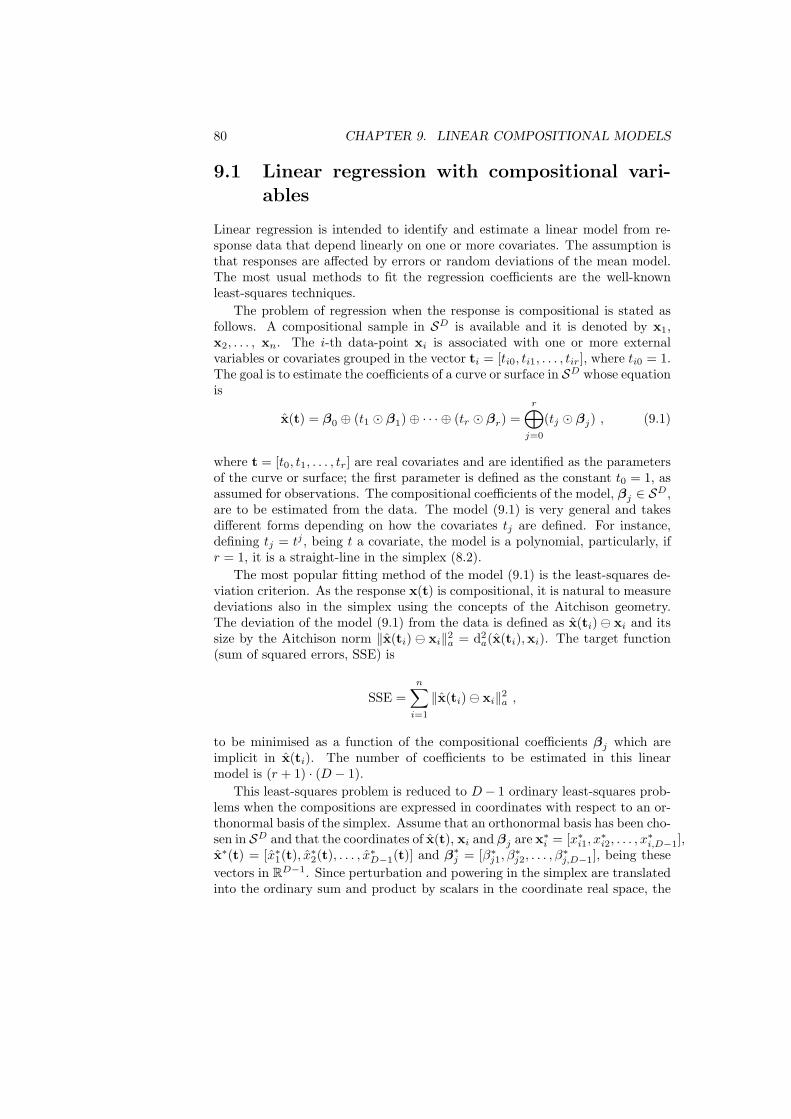
80 CHAPTER 9. LINEAR COMPOSITIONAL MODELS
9.1 Linear regression with compositional vari-ables
Linear regression is intended to identify and estimate a linear model from re-sponse data that depend linearly on one or more covariates. The assumption isthat responses are affected by errors or random deviations of the mean model.The most usual methods to fit the regression coefficients are the well-knownleast-squares techniques.
The problem of regression when the response is compositional is stated asfollows. A compositional sample in SD is available and it is denoted by x1,x2, . . . , xn. The i-th data-point xi is associated with one or more externalvariables or covariates grouped in the vector ti = [ti0, ti1, . . . , tir], where ti0 = 1.The goal is to estimate the coefficients of a curve or surface in SD whose equationis
x(t) = β0 ⊕ (t1 ¯ β1)⊕ · · · ⊕ (tr ¯ βr) =r⊕
j=0
(tj ¯ βj) , (9.1)
where t = [t0, t1, . . . , tr] are real covariates and are identified as the parametersof the curve or surface; the first parameter is defined as the constant t0 = 1, asassumed for observations. The compositional coefficients of the model, βj ∈ SD,are to be estimated from the data. The model (9.1) is very general and takesdifferent forms depending on how the covariates tj are defined. For instance,defining tj = tj , being t a covariate, the model is a polynomial, particularly, ifr = 1, it is a straight-line in the simplex (8.2).
The most popular fitting method of the model (9.1) is the least-squares de-viation criterion. As the response x(t) is compositional, it is natural to measuredeviations also in the simplex using the concepts of the Aitchison geometry.The deviation of the model (9.1) from the data is defined as x(ti)ª xi and itssize by the Aitchison norm ‖x(ti) ª xi‖2a = d2
a(x(ti),xi). The target function(sum of squared errors, SSE) is
SSE =n∑
i=1
‖x(ti)ª xi‖2a ,
to be minimised as a function of the compositional coefficients βj which areimplicit in x(ti). The number of coefficients to be estimated in this linearmodel is (r + 1) · (D − 1).
This least-squares problem is reduced to D− 1 ordinary least-squares prob-lems when the compositions are expressed in coordinates with respect to an or-thonormal basis of the simplex. Assume that an orthonormal basis has been cho-sen in SD and that the coordinates of x(t), xi and βj are x∗i = [x∗i1, x
∗i2, . . . , x
∗i,D−1],
x∗(t) = [x∗1(t), x∗2(t), . . . , x
∗D−1(t)] and β∗j = [β∗j1, β
∗j2, . . . , β
∗j,D−1], being these
vectors in RD−1. Since perturbation and powering in the simplex are translatedinto the ordinary sum and product by scalars in the coordinate real space, the
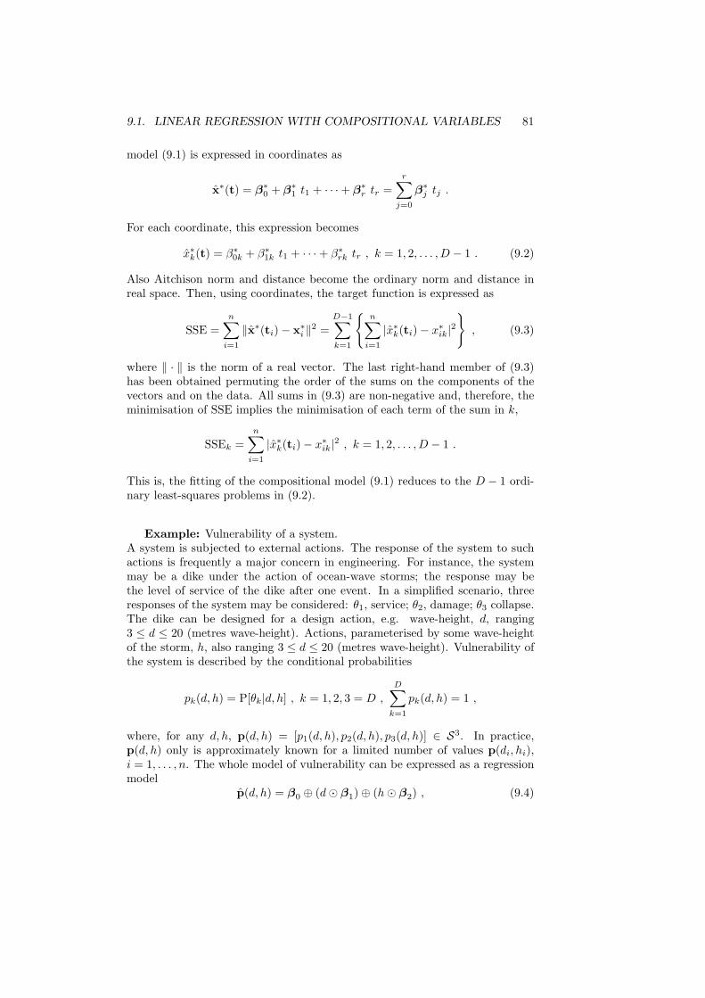
9.1. LINEAR REGRESSION WITH COMPOSITIONAL VARIABLES 81
model (9.1) is expressed in coordinates as
x∗(t) = β∗0 + β∗1 t1 + · · ·+ β∗r tr =r∑
j=0
β∗j tj .
For each coordinate, this expression becomes
x∗k(t) = β∗0k + β∗1k t1 + · · ·+ β∗rk tr , k = 1, 2, . . . , D − 1 . (9.2)
Also Aitchison norm and distance become the ordinary norm and distance inreal space. Then, using coordinates, the target function is expressed as
SSE =n∑
i=1
‖x∗(ti)− x∗i ‖2 =D−1∑
k=1
{n∑
i=1
|x∗k(ti)− x∗ik|2}
, (9.3)
where ‖ · ‖ is the norm of a real vector. The last right-hand member of (9.3)has been obtained permuting the order of the sums on the components of thevectors and on the data. All sums in (9.3) are non-negative and, therefore, theminimisation of SSE implies the minimisation of each term of the sum in k,
SSEk =n∑
i=1
|x∗k(ti)− x∗ik|2 , k = 1, 2, . . . , D − 1 .
This is, the fitting of the compositional model (9.1) reduces to the D − 1 ordi-nary least-squares problems in (9.2).
Example: Vulnerability of a system.A system is subjected to external actions. The response of the system to suchactions is frequently a major concern in engineering. For instance, the systemmay be a dike under the action of ocean-wave storms; the response may bethe level of service of the dike after one event. In a simplified scenario, threeresponses of the system may be considered: θ1, service; θ2, damage; θ3 collapse.The dike can be designed for a design action, e.g. wave-height, d, ranging3 ≤ d ≤ 20 (metres wave-height). Actions, parameterised by some wave-heightof the storm, h, also ranging 3 ≤ d ≤ 20 (metres wave-height). Vulnerability ofthe system is described by the conditional probabilities
pk(d, h) = P[θk|d, h] , k = 1, 2, 3 = D ,
D∑
k=1
pk(d, h) = 1 ,
where, for any d, h, p(d, h) = [p1(d, h), p2(d, h), p3(d, h)] ∈ S3. In practice,p(d, h) only is approximately known for a limited number of values p(di, hi),i = 1, . . . , n. The whole model of vulnerability can be expressed as a regressionmodel
p(d, h) = β0 ⊕ (d¯ β1)⊕ (h¯ β2) , (9.4)
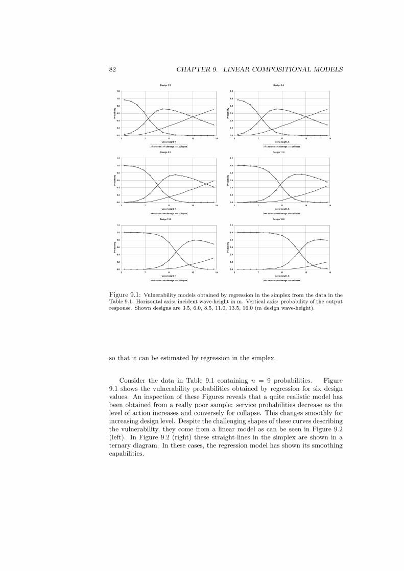
82 CHAPTER 9. LINEAR COMPOSITIONAL MODELS
Design 3.5
0.0
0.2
0.4
0.6
0.8
1.0
1.2
3 7 11 15 19
wave-height, h
Pro
ba
bil
ity
service damage collapse
Design 6.0
0.0
0.2
0.4
0.6
0.8
1.0
1.2
3 7 11 15 19
wave-height, h
Pro
ba
bil
ity
service damage collapse
Design 8.5
0.0
0.2
0.4
0.6
0.8
1.0
1.2
3 7 11 15 19
wave-height, h
Pro
ba
bil
ity
service damage collapse
Design 11.0
0.0
0.2
0.4
0.6
0.8
1.0
1.2
3 7 11 15 19
wave-height, h
Pro
ba
bil
ity
service damage collapse
Design 13.5
0.0
0.2
0.4
0.6
0.8
1.0
1.2
3 7 11 15 19
wave-height, h
Pro
ba
bil
ity
service damage collapse
Design 16.0
0.0
0.2
0.4
0.6
0.8
1.0
1.2
3 7 11 15 19
wave-height, h
Pro
ba
bil
ity
service damage collapse
Figure 9.1: Vulnerability models obtained by regression in the simplex from the data in theTable 9.1. Horizontal axis: incident wave-height in m. Vertical axis: probability of the outputresponse. Shown designs are 3.5, 6.0, 8.5, 11.0, 13.5, 16.0 (m design wave-height).
so that it can be estimated by regression in the simplex.
Consider the data in Table 9.1 containing n = 9 probabilities. Figure9.1 shows the vulnerability probabilities obtained by regression for six designvalues. An inspection of these Figures reveals that a quite realistic model hasbeen obtained from a really poor sample: service probabilities decrease as thelevel of action increases and conversely for collapse. This changes smoothly forincreasing design level. Despite the challenging shapes of these curves describingthe vulnerability, they come from a linear model as can be seen in Figure 9.2(left). In Figure 9.2 (right) these straight-lines in the simplex are shown in aternary diagram. In these cases, the regression model has shown its smoothingcapabilities.
9.2. REGRESSION WITH COMPOSITIONAL COVARIATES 83
-2
-1
0
1
2
3
4
-10 -8 -6 -4 -2 0 2 4 6 8 10
6^(1/2) ln(p0^2/ p1 p2)
2^
(1/2
) ln
(p1/p
2)
service
damage collapse
Figure 9.2: Vulnerability models in Figure 9.1 in coordinates (left) and in the ternarydiagram (right). Design 3.5 (circles); 16.0 (thick line).
9.2 Regression with compositional covariates
The model with compositional covariates appears when the goal is to predict oneexternal variable as a function of a composition. Assume a compositional dataset x1, x2, . . . , xn is available, and that the i-th data-point xi is associated withan observation yi of an external response variable (with support the whole realline, i.e. possibly transformed with logs or any other suitable transformation).The goal is to estimate a surface on SD × R with equation
y(x) = β0 + 〈β,x〉a (9.5)
where β ∈ SD is the (simplicial) gradient of y with respect to x, and β0 is areal intercept. In this case, since the response is a real value, the classical leastsquares fitting criterion may be applied, which yields the target function
SSE =n∑
i=1
(yi − β0 − 〈β,xi〉a)2 .
As the Aitchison inner product can be computed easily from clr coefficients orilr coordinates of xi, this sum of squares becomes
SSE =n∑
i=1
(yi − β0 − 〈clr(β), clr(xi)〉)2 =n∑
i=1
(yi − β0 − 〈ilr(β), ilr(xi)〉)2.
This suggests that the actual fitting can be done using ilr coordinates withoutfurther ado. One simply fits a linear regression to the response y as a linearfunction of ilr(x). The estimated version of ilr(β) contains slope coefficients ofthe response y with respect the coordinates ilr(x). The simplicial gradient β isthen easily computed using ilr−1. The clr transformation should be avoided inthis case, as its correct handling in the scope of regression requires the gener-alized inversion of singular matrices (something that most statistical packagesare not able to do).
84 CHAPTER 9. LINEAR COMPOSITIONAL MODELS
Tests on the coefficients of the model (9.5) may be used as usual, for instanceto obtain a simplified model depending on less variables. However, one shouldbe aware that they are related to the particular basis used, and that thesesimplified models will be different depending on the basis. One should thuscarefully select the basis: for instance, a basis of balances may be adequate tocheck the dependence of y on a particular subcomposition of x.
Exercise 9.2.1 (sand-silt-clay from a lake) Consider the data in Table9.2. They are sand-silt-clay compositions from an Arctic lake taken at differentdepths (adapted from Coakley and Rust (1968) and cited in Aitchison (1986)).The goal is to check whether there is some trend in the composition related to thedepth. Particularly, using the standard hypothesis testing in regression, checkthe constant and the straight-line models
x(t) = β0 , x(t) = β0 ⊕ (t¯ β1) ,
being t =depth. Plot both models, the fitted model and the residuals, in coordi-nates and in the ternary diagram.
Exercise 9.2.2 (sand-silt-clay from a lake: second sight) One can equiv-alently check whether the sediment composition brings any information about thedepth at which that sample was taken. Using the data from the previous excer-cise, fit a linear model to explain depth as a function of the composition. Analysethe residuals as usual, as they may be considered real values.
To display the model, you can follow these steps. Split the range of observeddepths in several segments of the same length (four to six will be enough in Co-DaPack), and give each sample a number corresponding to its depth cathegory.Plot the compositional data in a ternary diagram, using colors for each depthinterval. Draw a line on the simplex, from the center of the data set along thegradient of the fitted model
9.3 Analysis of variance with compositional re-sponse
ANalysis Of the VAriance (ANOVA) is the name given to a linear model wherea continuous response is explained as a function of a (set of) discrete variable(s).Compositional ANOVA follows the same steps that were used to predict a com-position from a continuous covariable. Notation in multi-way ANOVA (withmore than one discrete covariable) can become quite difficult, therefore onlyone-way compositional ANOVA will be addressed here. Textbooks on multi-variate ANOVA may be then useful to extend this material.
As in the preceding section, assume a compositional sample x1, x2, . . . , xn
in SD is available. These observations are classified into K categories across anexternal categorical variable z. Category z may represent different treatments
9.3. ANALYSIS OF VARIANCE WITH COMPOSITIONAL RESPONSE 85
or subpopulations. In other words, for each composition one has also availablea category zi. ANOVA deals with the centres (compositional means) of thecomposition for each category, µ1, . . . , µK . Following the classical notation, acompositional ANOVA model, for a given z, is
x = β1 ⊕ (I(z = 2))¯ β2)⊕ · · · ⊕ (I(z = K)¯ βK) ,xª x = ε,
where the indicator I(z = k) equals 1 when the condition is true and 0 otherwise.This means that only one of the K − 1 terms may be taken into account foreach possible z value (as the other will be powered by zero). Note that thefirst category does not explicitly appear in the equation: when z = 1, then thepredictor is only β1 = µ1 the centre of the first group. The remaining coefficientsare then interpreted as increments of the composition from the reference firstlevel to the category actually observed, x|k = µk = β1 ⊕ βk, or equivalentlyβk = µk ª µ1. The variable ε is the compositional residual of the model.
ANOVA notation may be quite cumbersome, but its fitting is straightfor-ward. For each observation zi one just constructs a vector ti with the K − 1indicators, i.e. with many zeroes and a single 1 in the position of the observedcategory. With these vectors, one applies the same steps as with linear regres-sion with compositional response (section 9.1). An important consequence ofthis procedure is that we implicitly assume equal total variance within eachcategory (compare with chapter 7).
The practice of compositional ANOVA follows the principle of working oncoordinates. One first selects a basis and computes the corresponding coordi-nates of the observations. Then classical ANOVA is applied to explain eachilr coordinate as a mean reference level plus K − 1 mean differences betweencategories. Tests may be applied to conclude that some of these differences arenot significative, i.e. that the mean of a particular coordinate at two categoriesmay be taken as equal. Finally, all coefficients associated with category k canbe back-transformed to obtain its associated compositional coefficient βk.
Exercise 9.3.1 (distinguishing mean rivers hydrogeochemistry) In thecourse accessory files you can find a file named “Hydrochem.csv”, containing anextensive data set of the geochemical composition of water samples from severalrivers and tributaries of the Llobregat river, the most important river in theBarcelona province (NE Spain). This data was studied in detail by Otero et al.(2005); Tolosana-Delgado et al. (2005), and placed, with the authors’ consent,in the public domain within the R package “compositions” (van den Boogaartand Tolosana-Delgado, 2008). Table 9.3 provides a random sample, in case thewhole data set is not accessible.
Fit an ANOVA model to this 3-part composition. Draw the data set usingcolours to distinguish between the four rivers. Plot the means of the four groups,as estimated by the ANOVA fit.
86 CHAPTER 9. LINEAR COMPOSITIONAL MODELS
Advanced excercise: Extract the variance-covariance matrix of each mean.Draw confidence regions for them, as explained in section B.
9.4 Linear discrimination with compositional pre-dictor
A composition can also be used to predict a categorical variable. Following thepreceding section notation, the goal is now to estimate p(x), the probability thatz takes each of its possible K values given an observed composition x. There aremany techniques to obtain this result, like the Fisher rule, linear or quadraticdiscriminant analysis, or multinomial logistic regression. But essentially, wewould always apply the principle of working on coordinates (take ilr’s, applyyour favourite method to the coordinates, and back-transform the coefficients ifthey may be interpreted as compositions). This section illustrates this procedurewith linear discriminant analysis (LDA), a technique available in most basicstatistical packages.
First, LDA assumes some prior probabilities p0k of data-points corresponding
to each one of the K categories. These are typically taken as pk = 1/K (equallyprobable) or pk = nk/n (where nk is the number of samples in kth-category).Then, it assumes that the ilr-transformed composition has a normal distribution,with ilr mean µ∗k = ilr(µk) and common ilr-coordinates covariance Σ (i.e., allcategories have the same covariance and possibly different mean). ApplyingBayes’ Theorem, it is verified that the posterior probability vector of belongingto each class for a particular composition x, can be derived from the discriminantfunctions
djk(x) = lnpj
pk= Aij + (µ∗j − µ∗k)′ ·Σ−1 · x∗.
with
Aij = lnp0
j
p0k
− 12(µ∗j − µ∗k)′ ·Σ−1 · (µ∗j − µ∗k)
Again, as happened with ANOVA, one category is typically placed as a sort ofreference level. For instance, take j = K fix. Then LDA just computes the log-odds of the the other K− 1 categories with respect to the last one. The desiredprobabilities can be obtained with the inverse alr transformation, as explainedin section 4.6.
Obtained probabilities can be then used to decide which category is moreprobable for each possible composition x: typically we classify each point in SD
into the most likely group, the one with largest probability. In this sense, thediscriminant functions can be used to draw the boundaries between regions jand k, by identifying the set of points where djk(x) = 0. Some linear algebrashows that this boundary is the affine hyperplane of SD orthogonal to the vector
9.4. LINEAR DISCRIMINATION WITH COMPOSITIONAL PREDICTOR87
vdj and passing through the point x0jk obtained as
vjk = [Σ−1 · (µ∗j − µ∗k)]
x0jk = (µ∗j + µ∗k)/2− Aij
2(µ∗j − µ∗k)′ · vjk· (µ∗j − µ∗k).
Note that these equations are only useful to draw boundaries between neigh-bouring categories, i.e. between the two most probable categories of a givenpoint in SD. For more than 2 categories, care should be taken to draw them bysegments.
Exercise 9.4.1 (drawing borders between three groups) Betweenthree groups we can draw three borders (A with B, B with C, A with C). Showthat these three boundaries intersect in one single point (a triple junction). Findthe equation of that point. Now assume that the discriminating compositionhas three components: note that in this case, the boundaries could be drawnas segments from the triple junction along the directions of some vectors v⊥jk
orthogonal to vjk.
Exercise 9.4.2 (the hydrochemical data set revisited) Using the dataset from exercise 9.3.1, obtain the discriminant functions between rivers A, Uand L (remove C for this exercise). This may be easily done by computing theilr coordinates in CoDaPack, and exporting them to your favourite statisticalsoftware. Draw the data in the ilr plane and in a ternary diagram, using coloursto distinguish between rivers. Add the group centers, and the boundaries betweengroups. If you use R, linear discriminant analysis is available with function“lda” in the package “MASS”.
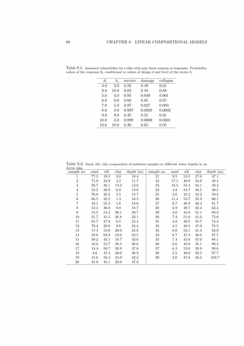
88 CHAPTER 9. LINEAR COMPOSITIONAL MODELS
Table 9.1: Assumed vulnerability for a dike with only three outputs or responses. Probabilityvalues of the response θk conditional to values of design d and level of the storm h.
di hi service damage collapse3.0 3.0 0.50 0.49 0.013.0 10.0 0.02 0.10 0.885.0 4.0 0.95 0.049 0.0016.0 9.0 0.08 0.85 0.077.0 5.0 0.97 0.027 0.0038.0 3.0 0.997 0.0028 0.00029.0 9.0 0.35 0.55 0.01
10.0 3.0 0.999 0.0009 0.000110.0 10.0 0.30 0.65 0.05
Table 9.2: Sand, silt, clay composition of sediment samples at different water depths in anArctic lake.sample no. sand silt clay depth (m) sample no. sand silt clay depth (m)
1 77.5 19.5 3.0 10.4 21 9.5 53.5 37.0 47.12 71.9 24.9 3.2 11.7 22 17.1 48.0 34.9 48.43 50.7 36.1 13.2 12.8 23 10.5 55.4 34.1 49.44 52.2 40.9 6.9 13.0 24 4.8 54.7 40.5 49.55 70.0 26.5 3.5 15.7 25 2.6 45.2 52.2 59.26 66.5 32.2 1.3 16.3 26 11.4 52.7 35.9 60.17 43.1 55.3 1.6 18.0 27 6.7 46.9 46.4 61.78 53.4 36.8 9.8 18.7 28 6.9 49.7 43.4 62.49 15.5 54.4 30.1 20.7 29 4.0 44.9 51.1 69.310 31.7 41.5 26.8 22.1 30 7.4 51.6 41.0 73.611 65.7 27.8 6.5 22.4 31 4.8 49.5 45.7 74.412 70.4 29.0 0.6 24.4 32 4.5 48.5 47.0 78.513 17.4 53.6 29.0 25.8 33 6.6 52.1 41.3 82.914 10.6 69.8 19.6 32.5 34 6.7 47.3 46.0 87.715 38.2 43.1 18.7 33.6 35 7.4 45.6 47.0 88.116 10.8 52.7 36.5 36.8 36 6.0 48.9 45.1 90.417 18.4 50.7 30.9 37.8 37 6.3 53.8 39.9 90.618 4.6 47.4 48.0 36.9 38 2.5 48.0 49.5 97.719 15.6 50.4 34.0 42.2 39 2.0 47.8 50.2 103.720 31.9 45.1 23.0 47.0
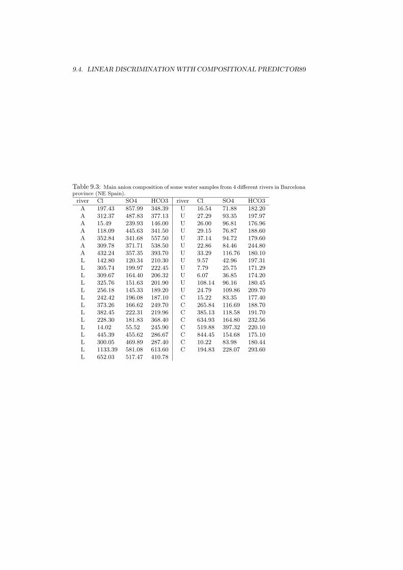
9.4. LINEAR DISCRIMINATION WITH COMPOSITIONAL PREDICTOR89
Table 9.3: Main anion composition of some water samples from 4 different rivers in Barcelonaprovince (NE Spain).
river Cl SO4 HCO3 river Cl SO4 HCO3
A 197.43 857.99 348.39 U 16.54 71.88 182.20A 312.37 487.83 377.13 U 27.29 93.35 197.97A 15.49 239.93 146.00 U 26.00 96.81 176.96A 118.09 445.63 341.50 U 29.15 76.87 188.60A 352.84 341.68 557.50 U 37.14 94.72 179.60A 309.78 371.71 538.50 U 22.86 84.46 244.80A 432.24 357.35 393.70 U 33.29 116.76 180.10L 142.80 120.34 210.30 U 9.57 42.96 197.31L 305.74 199.97 222.45 U 7.79 25.75 171.29L 309.67 164.40 206.32 U 6.07 36.85 174.20L 325.76 151.63 201.90 U 108.14 96.16 180.45L 256.18 145.33 189.20 U 24.79 109.86 209.70L 242.42 196.08 187.10 C 15.22 83.35 177.40L 373.26 166.62 249.70 C 265.84 116.69 188.70L 382.45 222.31 219.96 C 385.13 118.58 191.70L 228.30 181.83 368.40 C 634.93 164.80 232.56L 14.02 55.52 245.90 C 519.88 397.32 220.10L 445.39 455.62 286.67 C 844.45 154.68 175.10L 300.05 469.89 287.40 C 10.22 83.98 180.44L 1133.39 581.08 613.60 C 194.83 228.07 293.60L 652.03 517.47 410.78

90 CHAPTER 9. LINEAR COMPOSITIONAL MODELS
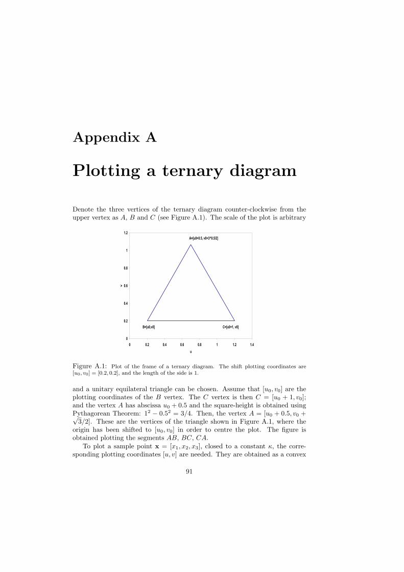
Appendix A
Plotting a ternary diagram
Denote the three vertices of the ternary diagram counter-clockwise from theupper vertex as A, B and C (see Figure A.1). The scale of the plot is arbitrary
0
0.2
0.4
0.6
0.8
1
1.2
0 0.2 0.4 0.6 0.8 1 1.2 1.4
u
v
A=[u0+0.5, v0+3^0.5/2]
B=[u0,v0] C=[u0+1, v0]
Figure A.1: Plot of the frame of a ternary diagram. The shift plotting coordinates are[u0, v0] = [0.2, 0.2], and the length of the side is 1.
and a unitary equilateral triangle can be chosen. Assume that [u0, v0] are theplotting coordinates of the B vertex. The C vertex is then C = [u0 + 1, v0];and the vertex A has abscissa u0 + 0.5 and the square-height is obtained usingPythagorean Theorem: 12 − 0.52 = 3/4. Then, the vertex A = [u0 + 0.5, v0 +√
3/2]. These are the vertices of the triangle shown in Figure A.1, where theorigin has been shifted to [u0, v0] in order to centre the plot. The figure isobtained plotting the segments AB, BC, CA.
To plot a sample point x = [x1, x2, x3], closed to a constant κ, the corre-sponding plotting coordinates [u, v] are needed. They are obtained as a convex
91

92 APPENDIX A. PLOTTING A TERNARY DIAGRAM
linear combination of the plotting coordinates of the vertices
[u, v] =1κ
(x1A + x2B + x3C) ,
withA = [u0 + 0.5, v0 +
√3/2] , B = [u0, v0] , C = [u0 + 1, v0] .
Note that the coefficients of the convex linear combination must be closed to1 as obtained dividing by κ. Deformed ternary diagrams can be obtained justchanging the plotting coordinates of the vertices and maintaining the convexlinear combination.
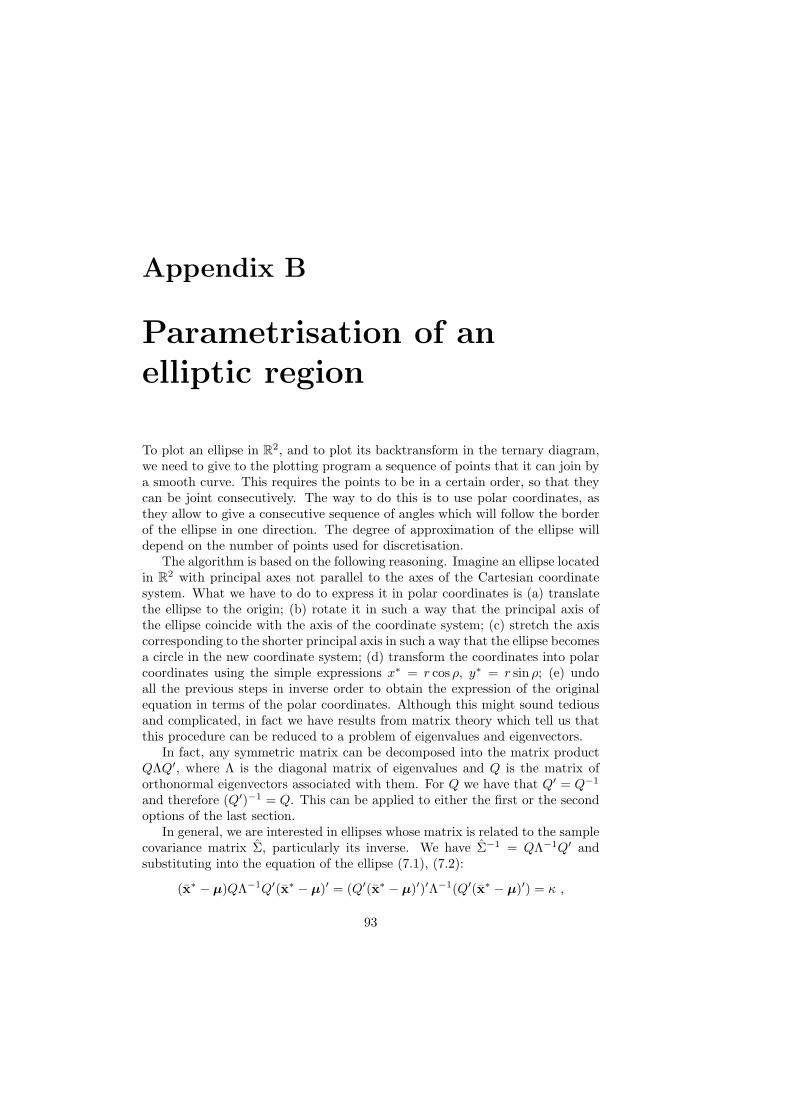
Appendix B
Parametrisation of anelliptic region
To plot an ellipse in R2, and to plot its backtransform in the ternary diagram,we need to give to the plotting program a sequence of points that it can join bya smooth curve. This requires the points to be in a certain order, so that theycan be joint consecutively. The way to do this is to use polar coordinates, asthey allow to give a consecutive sequence of angles which will follow the borderof the ellipse in one direction. The degree of approximation of the ellipse willdepend on the number of points used for discretisation.
The algorithm is based on the following reasoning. Imagine an ellipse locatedin R2 with principal axes not parallel to the axes of the Cartesian coordinatesystem. What we have to do to express it in polar coordinates is (a) translatethe ellipse to the origin; (b) rotate it in such a way that the principal axis ofthe ellipse coincide with the axis of the coordinate system; (c) stretch the axiscorresponding to the shorter principal axis in such a way that the ellipse becomesa circle in the new coordinate system; (d) transform the coordinates into polarcoordinates using the simple expressions x∗ = r cos ρ, y∗ = r sin ρ; (e) undoall the previous steps in inverse order to obtain the expression of the originalequation in terms of the polar coordinates. Although this might sound tediousand complicated, in fact we have results from matrix theory which tell us thatthis procedure can be reduced to a problem of eigenvalues and eigenvectors.
In fact, any symmetric matrix can be decomposed into the matrix productQΛQ′, where Λ is the diagonal matrix of eigenvalues and Q is the matrix oforthonormal eigenvectors associated with them. For Q we have that Q′ = Q−1
and therefore (Q′)−1 = Q. This can be applied to either the first or the secondoptions of the last section.
In general, we are interested in ellipses whose matrix is related to the samplecovariance matrix Σ, particularly its inverse. We have Σ−1 = QΛ−1Q′ andsubstituting into the equation of the ellipse (7.1), (7.2):
(x∗ − µ)QΛ−1Q′(x∗ − µ)′ = (Q′(x∗ − µ)′)′Λ−1(Q′(x∗ − µ)′) = κ ,
93
94 APPENDIX B. PARAMETRISATION OF AN ELLIPTIC REGION
where x∗ is the estimated centre or mean and µ describes the ellipse. The vectorQ′(x∗ −µ)′ corresponds to a rotation in real space in such a way, that the newcoordinate axis are precisely the eigenvectors. Given that Λ is a diagonal matrix,the next step consists in writing Λ−1 = Λ−1/2Λ−1/2, and we get:
(Q′(x∗ − µ)′)′Λ−1/2Λ−1/2(Q′(x∗ − µ)′)
= (Λ−1/2Q′(x∗ − µ)′)′(Λ−1/2Q′(x∗ − µ)′) = κ.
This transformation is equivalent to a re-scaling of the basis vectors in such away, that the ellipse becomes a circle of radius
√κ, which is easy to express in
polar coordinates:
Λ−1/2Q′(x∗ − µ)′ =(√
κ cos θ√κ sin θ
), or (x∗ − µ)′ = QΛ1/2
(√κ cos θ√κ sin θ
).
The parametrisation that we are looking for is thus given by:
µ′ = (x∗)′ −QΛ1/2
(√κ cos θ√κ sin θ
).
Note that QΛ1/2 is the upper triangular matrix of the Cholesky decompositionof Σ:
Σ = QΛ1/2Λ1/2Q′ = (QΛ1/2)(Λ1/2Q′) = UL;
thus, from Σ = UL and L = U ′ we get the condition:(
u11 u12
0 u22
)(u11 0u12 u22
)=
(Σ11 Σ12
Σ12 Σ22
),
which implies
u22 =√
Σ22,
u12 =Σ12√Σ22
,
u11 =
√Σ11Σ22 − Σ2
12
Σ22
=
√|Σ|Σ22
,
and for each component of the vector µ we obtain:
µ1 = x∗1 −√|Σ|Σ22
√κ cos θ − Σ12√
Σ22
√κ sin θ
µ2 = x∗2 −√
Σ22
√κ sin θ.
The points describing the ellipse in the simplex are ilr−1(µ) (see Section 4.4).The procedures described apply to the three cases studied in section 7.2,
just using the appropriate covariance matrix Σ. Finally, recall that κ will beobtained from a chi-square distribution.
Bibliography
Aitchison, J. (1981). A new approach to null correlations of proportions. Math-ematical Geology 13 (2), 175–189.
Aitchison, J. (1982). The statistical analysis of compositional data (with discus-sion). Journal of the Royal Statistical Society, Series B (Statistical Method-ology) 44 (2), 139–177.
Aitchison, J. (1983). Principal component analysis of compositional data.Biometrika 70 (1), 57–65.
Aitchison, J. (1984). The statistical analysis of geochemical compositions. Math-ematical Geology 16 (6), 531–564.
Aitchison, J. (1986). The Statistical Analysis of Compositional Data. Mono-graphs on Statistics and Applied Probability. Chapman & Hall Ltd., London(UK). (Reprinted in 2003 with additional material by The Blackburn Press).416 p.
Aitchison, J. (1990). Relative variation diagrams for describing patterns ofcompositional variability. Mathematical Geology 22 (4), 487–511.
Aitchison, J. (1997). The one-hour course in compositional data analysis or com-positional data analysis is simple. In V. Pawlowsky-Glahn (Ed.), Proceedingsof IAMG’97 — The third annual conference of the International Associationfor Mathematical Geology, Volume I, II and addendum, pp. 3–35. Interna-tional Center for Numerical Methods in Engineering (CIMNE), Barcelona(E), 1100 p.
Aitchison, J. (2002). Simplicial inference. In M. A. G. Viana and D. S. P.Richards (Eds.), Algebraic Methods in Statistics and Probability, Volume 287of Contemporary Mathematics Series, pp. 1–22. American Mathematical So-ciety, Providence, Rhode Island (USA), 340 p.
Aitchison, J., C. Barcelo-Vidal, J. J. Egozcue, and V. Pawlowsky-Glahn (2002).A concise guide for the algebraic-geometric structure of the simplex, thesample space for compositional data analysis. In U. Bayer, H. Burger, andW. Skala (Eds.), Proceedings of IAMG’02 — The eigth annual conference of
95
96 BIBLIOGRAPHY
the International Association for Mathematical Geology, Volume I and II, pp.387–392. Selbstverlag der Alfred-Wegener-Stiftung, Berlin, 1106 p.
Aitchison, J., C. Barcelo-Vidal, J. A. Martın-Fernandez, and V. Pawlowsky-Glahn (2000). Logratio analysis and compositional distance. MathematicalGeology 32 (3), 271–275.
Aitchison, J. and J. J. Egozcue (2005). Compositional data analysis: where arewe and where should we be heading? Mathematical Geology 37 (7), 829–850.
Aitchison, J. and M. Greenacre (2002). Biplots for compositional data. Journalof the Royal Statistical Society, Series C (Applied Statistics) 51 (4), 375–392.
Aitchison, J. and J. W. Kay (2003). Possible solution of some essential zeroproblems in compositional data analysis. See Thio-Henestrosa and Martın-Fernandez (2003).
Albarede, F. (1995). Introduction to geochemical modeling. Cambridge Univer-sity Press (UK). 543 p.
Anderson, T. W. (1984). An introduction to multivariate statistical analysis.Second ed., John Wiley and Sons, New York, USA.
Bacon-Shone, J. (2003). Modelling structural zeros in compositional data. SeeThio-Henestrosa and Martın-Fernandez (2003).
Barcelo, C., V. Pawlowsky, and E. Grunsky (1994). Outliers in compositionaldata: a first approach. In C. J. Chung (Ed.), Papers and extended abstractsof IAMG’94 — The First Annual Conference of the International Associa-tion for Mathematical Geology, Mont Tremblant, Quebec, Canada, pp. 21–26.IAMG.
Barcelo, C., V. Pawlowsky, and E. Grunsky (1996). Some aspects of transfor-mations of compositional data and the identification of outliers. MathematicalGeology 28 (4), 501–518.
Barcelo-Vidal, C., J. A. Martın-Fernandez, and V. Pawlowsky-Glahn (2001).Mathematical foundations of compositional data analysis. In G. Ross (Ed.),Proceedings of IAMG’01 — The sixth annual conference of the InternationalAssociation for Mathematical Geology, pp. 20 p. CD-ROM.
Billheimer, D., P. Guttorp, and W. Fagan (1997). Statistical analysis and inter-pretation of discrete compositional data. Technical report, NRCSE technicalreport 11, University of Washington, Seattle (USA), 48 p.
Billheimer, D., P. Guttorp, and W. Fagan (2001). Statistical interpretation ofspecies composition. Journal of the American Statistical Association 96 (456),1205–1214.
BIBLIOGRAPHY 97
Box, G. E. P. and D. R. Cox (1964). The analysis of transformations. Journal ofthe Royal Statistical Society, Series B (Statistical Methodology) 26 (2), 211–252.
Buccianti, A. and V. Pawlowsky-Glahn (2005). New perspectives on waterchemistry and compositional data analysis. Mathematical Geology 37 (7), 703–727.
Buccianti, A., V. Pawlowsky-Glahn, C. Barcelo-Vidal, and E. Jarauta-Bragulat(1999). Visualization and modeling of natural trends in ternary diagrams: ageochemical case study. See Lippard et al. (1999), pp. 139–144.
Chayes, F. (1960). On correlation between variables of constant sum. Journalof Geophysical Research 65 (12), 4185–4193.
Chayes, F. (1971). Ratio Correlation. University of Chicago Press, Chicago, IL(USA). 99 p.
Coakley, J. P. and B. R. Rust (1968). Sedimentation in an Arctic lake. Journalof Sedimentary Petrology 38, 1290–1300.
Eaton, M. L. (1983). Multivariate Statistics. A Vector Space Approach. JohnWiley & Sons.
Egozcue, J. J. (2009). Reply to ”On the Harker variation diagrams; ...” by J.A. Cortes. Mathematical Geosciences 41 (7), 829–834.
Egozcue, J. J. and V. Pawlowsky-Glahn (2005). Groups of parts and theirbalances in compositional data analysis. Mathematical Geology 37 (7), 795–828.
Egozcue, J. J. and V. Pawlowsky-Glahn (2006). Exploring compositional datawith the coda-dendrogram. In E. Pirard (Ed.), Proceedings of IAMG’06 —The XIth annual conference of the International Association for MathematicalGeology.
Egozcue, J. J., V. Pawlowsky-Glahn, G. Mateu-Figueras, and C. Barcelo-Vidal(2003). Isometric logratio transformations for compositional data analysis.Mathematical Geology 35 (3), 279–300.
Fahrmeir, L. and A. Hamerle (Eds.) (1984). Multivariate Statistische Verfahren.Walter de Gruyter, Berlin (D), 796 p.
Fry, J. M., T. R. L. Fry, and K. R. McLaren (1996). Compositional data analysisand zeros in micro data. Centre of Policy Studies (COPS), General Paper No.G-120, Monash University.
Gabriel, K. R. (1971). The biplot — graphic display of matrices with applicationto principal component analysis. Biometrika 58 (3), 453–467.
98 BIBLIOGRAPHY
Galton, F. (1879). The geometric mean, in vital and social statistics. Proceedingsof the Royal Society of London 29, 365–366.
Krzanowski, W. J. (1988). Principles of Multivariate Analysis: A user’s perspec-tive, Volume 3 of Oxford Statistical Science Series. Clarendon Press, Oxford(UK). 563 p.
Krzanowski, W. J. and F. H. C. Marriott (1994). Multivariate Analysis, Part 2- Classification, covariance structures and repeated measurements, Volume 2of Kendall’s Library of Statistics. Edward Arnold, London (UK). 280 p.
Lippard, S. J., A. Næss, and R. Sinding-Larsen (Eds.) (1999). Proceedings ofIAMG’99 — The fifth annual conference of the International Association forMathematical Geology, Volume I and II. Tapir, Trondheim (N), 784 p.
Mardia, K. V., J. T. Kent, and J. M. Bibby (1979). Multivariate Analysis.Academic Press, London (GB). 518 p.
Martın-Fernandez, J., C. Barcelo-Vidal, and V. Pawlowsky-Glahn (1998). Acritical approach to non-parametric classification of compositional data. InA. Rizzi, M. Vichi, and H.-H. Bock (Eds.), Advances in Data Science andClassification (Proceedings of the 6th Conference of the International Federa-tion of Classification Societies (IFCS’98), Universita “La Sapienza”, Rome,21–24 July, pp. 49–56. Springer-Verlag, Berlin (D), 677 p.
Martın-Fernandez, J. A. (2001). Medidas de diferencia y clasificacion noparametrica de datos composicionales. Ph. D. thesis, Universitat Politecnicade Catalunya, Barcelona (E).
Martın-Fernandez, J. A., C. Barcelo-Vidal, and V. Pawlowsky-Glahn (2000).Zero replacement in compositional data sets. In H. Kiers, J. Rasson, P. Groe-nen, and M. Shader (Eds.), Studies in Classification, Data Analysis, andKnowledge Organization (Proceedings of the 7th Conference of the Interna-tional Federation of Classification Societies (IFCS’2000), University of Na-mur, Namur, 11-14 July, pp. 155–160. Springer-Verlag, Berlin (D), 428 p.
Martın-Fernandez, J. A., C. Barcelo-Vidal, and V. Pawlowsky-Glahn (2003).Dealing with zeros and missing values in compositional data sets using non-parametric imputation. Mathematical Geology 35 (3), 253–278.
Martın-Fernandez, J. A., M. Bren, C. Barcelo-Vidal, and V. Pawlowsky-Glahn(1999). A measure of difference for compositional data based on measures ofdivergence. See Lippard et al. (1999), pp. 211–216.
Mateu-Figueras, G. (2003). Models de distribucio sobre el sımplex. Ph. D. thesis,Universitat Politecnica de Catalunya, Barcelona, Spain.
McAlister, D. (1879). The law of the geometric mean. Proceedings of the RoyalSociety of London 29, 367–376.

BIBLIOGRAPHY 99
Mosimann, J. E. (1962). On the compound multinomial distribution, the multi-variate β-distribution and correlations among proportions. Biometrika 49 (1-2), 65–82.
Otero, N., R. Tolosana-Delgado, and A. Soler (2003). A factor analysis ofhidrochemical composition of Llobregat river basin. See Thio-Henestrosa andMartın-Fernandez (2003).
Otero, N., R. Tolosana-Delgado, A. Soler, V. Pawlowsky-Glahn, and A. Canals(2005). Relative vs. absolute statistical analysis of compositions: a compar-ative study of surface waters of a mediterranean river. Water Research Vol39 (7), 1404–1414.
Pawlowsky-Glahn, V. (2003). Statistical modelling on coordinates. See Thio-Henestrosa and Martın-Fernandez (2003).
Pawlowsky-Glahn, V. and A. Buccianti (2002). Visualization and modelingof subpopulations of compositional data: statistical methods illustrated bymeans of geochemical data from fumarolic fluids. International Journal ofEarth Sciences (Geologische Rundschau) 91 (2), 357–368.
Pawlowsky-Glahn, V. and J. J. Egozcue (2001). Geometric approach to statis-tical analysis on the simplex. Stochastic Environmental Research and RiskAssessment (SERRA) 15 (5), 384–398.
Pawlowsky-Glahn, V. and J. J. Egozcue (2002). BLU estimators and composi-tional data. Mathematical Geology 34 (3), 259–274.
Pawlowsky-Glahn, V. and J. J. Egozcue (2006). Anlisis de datos composicionalescon el coda-dendrograma. In J. Sicilia-Rodrıguez, C. Gonzalez-Martın, M. A.Gonzalez-Sierra, and D. Alcaide (Eds.), Actas del XXIX Congreso de la So-ciedad de Estadıstica e Investigacion Operativa (SEIO’06), pp. 39–40. So-ciedad de Estadıstica e Investigacion Operativa, Tenerife (ES), CD-ROM.
Pena, D. (2002). Analisis de datos multivariantes. McGraw Hill. 539 p.
Pearson, K. (1897). Mathematical contributions to the theory of evolution.on a form of spurious correlation which may arise when indices are used inthe measurement of organs. Proceedings of the Royal Society of London LX,489–502.
Richter, D. H. and J. G. Moore (1966). Petrology of the Kilauea Iki lava lake,Hawaii. U.S. Geol. Surv. Prof. Paper 537-B, B1-B26, cited in Rollinson (1995).
Rollinson, H. R. (1995). Using geochemical data: Evaluation, presentation,interpretation. Longman Geochemistry Series, Longman Group Ltd., Essex(UK). 352 p.
Sarmanov, O. V. and A. B. Vistelius (1959). On the correlation of percentagevalues. Doklady of the Academy of Sciences of the USSR – Earth SciencesSection 126, 22–25.
100 BIBLIOGRAPHY
Solano-Acosta, W. and P. K. Dutta (2005). Unexpected trend in the composi-tional maturity of second-cycle sand. Sedimentary Geology 178 (3-4), 275–283.
Thio-Henestrosa, S. and J. A. Martın-Fernandez (Eds.) (2003). Composi-tional Data Analysis Workshop – CoDaWork’03, Proceedings. Universitat deGirona, ISBN 84-8458-111-X, http://ima.udg.es/Activitats/CoDaWork03/.
Thio-Henestrosa, S. and J. A. Martın-Fernandez (2005). Dealing with compo-sitional data: the freeware codapack. Mathematical Geology 37 (7), 773–793.
Thio-Henestrosa, S., R. Tolosana-Delgado, and O. Gomez (2005). New featuresof codapack—a compositional data package. Volume 2, pp. 1171–1178.
Tolosana-Delgado, R., N. Otero, V. Pawlowsky-Glahn, and A. Soler (2005). La-tent compositional factors in the Llobregat river basin (Spain) hydrogeoeo-chemistry. Mathematical Geology 37 (7), 681–702.
van den Boogaart, G. and R. Tolosana-Delgado (2005). A compositionaldata analysis package for R providing multiple approaches. In G. Mateu-Figueras and C. Barcelo-Vidal (Eds.), Compositional Data Analysis Workshop– CoDaWork’05, Proceedings. Universitat de Girona, ISBN 84-8458-222-1,http://ima.udg.es/Activitats/CoDaWork05/.
van den Boogaart, K. G. and R. Tolosana-Delgado (2008). “compositions”:a unified R package to analyze compositional data. Computers & Geo-sciences 34 (4), 320–338.
von Eynatten, H., V. Pawlowsky-Glahn, and J. J. Egozcue (2002). Understand-ing perturbation on the simplex: a simple method to better visualise and in-terpret compositional data in ternary diagrams. Mathematical Geology 34 (3),249–257.