Embed Size (px)
Citation preview
Lecture Notes on Real AnalysisUniversite Pierre et Marie Curie (Paris 6)
Nicolas Lerner
September 18, 2017

2
Contents
1 Basic structures: topology, metrics 71.1 Topological spaces . . . . . . . . . . . . . . . . . . . . . . . . . . . . 71.2 Metric Spaces . . . . . . . . . . . . . . . . . . . . . . . . . . . . . . . 111.3 Topological Vector Spaces . . . . . . . . . . . . . . . . . . . . . . . . 13
1.3.1 General definitions . . . . . . . . . . . . . . . . . . . . . . . . 131.3.2 Vector spaces with a translation-invariant distance . . . . . . . 141.3.3 Normed spaces . . . . . . . . . . . . . . . . . . . . . . . . . . 151.3.4 Semi-norms . . . . . . . . . . . . . . . . . . . . . . . . . . . . 18
1.4 A review of the basic structures for TVS . . . . . . . . . . . . . . . . 211.4.1 Hilbert spaces . . . . . . . . . . . . . . . . . . . . . . . . . . . 211.4.2 Banach spaces . . . . . . . . . . . . . . . . . . . . . . . . . . . 211.4.3 Frechet spaces . . . . . . . . . . . . . . . . . . . . . . . . . . . 221.4.4 More general structures . . . . . . . . . . . . . . . . . . . . . 22
1.5 Compactness . . . . . . . . . . . . . . . . . . . . . . . . . . . . . . . 221.5.1 Compact topological spaces . . . . . . . . . . . . . . . . . . . 221.5.2 Compact metric spaces . . . . . . . . . . . . . . . . . . . . . . 231.5.3 Local compactness . . . . . . . . . . . . . . . . . . . . . . . . 27
2 Basic tools of Functional Analysis 312.1 The Baire theorem and its consequences . . . . . . . . . . . . . . . . 31
2.1.1 The Baire category theorem . . . . . . . . . . . . . . . . . . . 312.1.2 The Banach-Steinhaus theorem . . . . . . . . . . . . . . . . . 342.1.3 The open mapping theorem . . . . . . . . . . . . . . . . . . . 392.1.4 The closed graph theorem . . . . . . . . . . . . . . . . . . . . 41
2.2 The Hahn-Banach theorem . . . . . . . . . . . . . . . . . . . . . . . . 422.2.1 The Hahn-Banach theorem, Zorn’s lemma . . . . . . . . . . . 422.2.2 Corollary on the topological dual . . . . . . . . . . . . . . . . 45
2.3 Examples of Topological Vector Spaces . . . . . . . . . . . . . . . . . 462.3.1 C0(Ω), Ω open subset of Rn. . . . . . . . . . . . . . . . . . . . 462.3.2 Cm(Ω), Ω open subset of Rn, m ∈ N. . . . . . . . . . . . . . . 472.3.3 C∞(Ω), Ω open subset of Rn. . . . . . . . . . . . . . . . . . . 482.3.4 The space of holomorphic functions H(Ω), Ω open subset of C. 482.3.5 The Schwartz space S (Rn) of rapidly decreasing functions. . . 49
2.4 Ascoli’s theorem . . . . . . . . . . . . . . . . . . . . . . . . . . . . . . 492.4.1 An example and the statement . . . . . . . . . . . . . . . . . 492.4.2 The diagonal process . . . . . . . . . . . . . . . . . . . . . . . 51
3
4 CONTENTS
2.5 Duality in Banach spaces . . . . . . . . . . . . . . . . . . . . . . . . . 53
2.5.1 Definitions . . . . . . . . . . . . . . . . . . . . . . . . . . . . . 53
2.5.2 Weak convergence on E . . . . . . . . . . . . . . . . . . . . . 54
2.5.3 Weak-∗ convergence on E∗ . . . . . . . . . . . . . . . . . . . . 56
2.5.4 Reflexivity . . . . . . . . . . . . . . . . . . . . . . . . . . . . . 58
2.5.5 Examples . . . . . . . . . . . . . . . . . . . . . . . . . . . . . 60
2.5.6 The dual of Lp(X,M, µ), 1 ≤ p < +∞. . . . . . . . . . . . . . 62
2.5.7 Transposition . . . . . . . . . . . . . . . . . . . . . . . . . . . 65
2.6 Appendix . . . . . . . . . . . . . . . . . . . . . . . . . . . . . . . . . 66
2.6.1 Filters . . . . . . . . . . . . . . . . . . . . . . . . . . . . . . . 66
3 Introduction to the Theory of Distributions 67
3.1 Test Functions and Distributions . . . . . . . . . . . . . . . . . . . . 67
3.1.1 Smooth compactly supported functions . . . . . . . . . . . . . 67
3.1.2 Distributions . . . . . . . . . . . . . . . . . . . . . . . . . . . 70
3.1.3 First examples of distributions . . . . . . . . . . . . . . . . . . 71
3.1.4 Continuity properties . . . . . . . . . . . . . . . . . . . . . . . 72
3.1.5 Partitions of unity and localization . . . . . . . . . . . . . . . 74
3.1.6 Weak convergence of distributions . . . . . . . . . . . . . . . . 75
3.2 Differentiation, multiplication by smooth functions . . . . . . . . . . 76
3.2.1 Differentiation . . . . . . . . . . . . . . . . . . . . . . . . . . . 76
3.2.2 Examples . . . . . . . . . . . . . . . . . . . . . . . . . . . . . 77
3.2.3 Product by smooth functions . . . . . . . . . . . . . . . . . . 79
3.2.4 Division of distribution on R by xm . . . . . . . . . . . . . . . 80
3.3 Distributions with compact support . . . . . . . . . . . . . . . . . . . 81
3.3.1 Identification with E ′ . . . . . . . . . . . . . . . . . . . . . . . 81
3.3.2 Distributions with support at a point . . . . . . . . . . . . . . 82
3.4 Tensor products . . . . . . . . . . . . . . . . . . . . . . . . . . . . . . 83
3.4.1 Differentiation of a duality product . . . . . . . . . . . . . . . 84
3.4.2 Pull-back by the affine group . . . . . . . . . . . . . . . . . . 85
3.4.3 Homogeneous distributions . . . . . . . . . . . . . . . . . . . . 85
3.4.4 Tensor products of distributions . . . . . . . . . . . . . . . . . 87
3.5 Convolution . . . . . . . . . . . . . . . . . . . . . . . . . . . . . . . . 91
3.5.1 Convolution E ′(Rn) ∗D ′(Rn) . . . . . . . . . . . . . . . . . . 91
3.5.2 Regularization . . . . . . . . . . . . . . . . . . . . . . . . . . . 92
3.5.3 Convolution with a proper support condition . . . . . . . . . . 94
3.6 Some fundamental solutions . . . . . . . . . . . . . . . . . . . . . . . 95
3.6.1 Definitions . . . . . . . . . . . . . . . . . . . . . . . . . . . . . 95
3.6.2 The Laplace and Cauchy-Riemann equations . . . . . . . . . . 96
3.6.3 Hypoellipticity . . . . . . . . . . . . . . . . . . . . . . . . . . 98
3.7 Appendix . . . . . . . . . . . . . . . . . . . . . . . . . . . . . . . . . 99
3.7.1 The Gamma function . . . . . . . . . . . . . . . . . . . . . . . 99
CONTENTS 5
4 Introduction to Fourier Analysis 1014.1 Fourier Transform of tempered distributions . . . . . . . . . . . . . . 101
4.1.1 The Fourier transformation on S (Rn) . . . . . . . . . . . . . 1014.1.2 The Fourier transformation on S ′(Rn) . . . . . . . . . . . . . 1044.1.3 The Fourier transformation on L1(Rn) . . . . . . . . . . . . . 1054.1.4 The Fourier transformation on L2(Rn) . . . . . . . . . . . . . 1054.1.5 Some standard examples of Fourier transform . . . . . . . . . 105
4.2 The Poisson summation formula . . . . . . . . . . . . . . . . . . . . . 1064.2.1 Wave packets . . . . . . . . . . . . . . . . . . . . . . . . . . . 1064.2.2 Poisson’s formula . . . . . . . . . . . . . . . . . . . . . . . . . 108
4.3 Fourier transformation and convolution . . . . . . . . . . . . . . . . . 1094.3.1 Fourier transformation on E ′(Rn) . . . . . . . . . . . . . . . . 1094.3.2 Convolution and Fourier transformation . . . . . . . . . . . . 1104.3.3 The Riemann-Lebesgue lemma . . . . . . . . . . . . . . . . . 111
4.4 Some fundamental solutions . . . . . . . . . . . . . . . . . . . . . . . 1114.4.1 The heat equation . . . . . . . . . . . . . . . . . . . . . . . . 1114.4.2 The Schrodinger equation . . . . . . . . . . . . . . . . . . . . 1134.4.3 The wave equation . . . . . . . . . . . . . . . . . . . . . . . . 115
4.5 Periodic distributions . . . . . . . . . . . . . . . . . . . . . . . . . . . 1194.5.1 The Dirichlet kernel . . . . . . . . . . . . . . . . . . . . . . . 1194.5.2 Pointwise convergence of Fourier series . . . . . . . . . . . . . 1204.5.3 Periodic distributions . . . . . . . . . . . . . . . . . . . . . . . 121
4.6 Appendix . . . . . . . . . . . . . . . . . . . . . . . . . . . . . . . . . 1244.6.1 The logarithm of a nonsingular symmetric matrix . . . . . . . 1244.6.2 Fourier transform of Gaussian functions . . . . . . . . . . . . 125
5 Analysis on Hilbert spaces 1275.1 Hilbert spaces . . . . . . . . . . . . . . . . . . . . . . . . . . . . . . . 127
5.1.1 Definitions and characterization . . . . . . . . . . . . . . . . . 1275.1.2 Projection on a closed convex set. Orthogonality . . . . . . . 1295.1.3 The Riesz representation theorem . . . . . . . . . . . . . . . . 1315.1.4 Hilbert basis . . . . . . . . . . . . . . . . . . . . . . . . . . . . 132
5.2 Bounded operators on a Hilbert space . . . . . . . . . . . . . . . . . . 1355.3 The Fourier transform on L2(Rn) . . . . . . . . . . . . . . . . . . . . 137
5.3.1 Plancherel formula . . . . . . . . . . . . . . . . . . . . . . . . 1375.3.2 Convolution of L2 functions . . . . . . . . . . . . . . . . . . . 138
5.4 Sobolev spaces . . . . . . . . . . . . . . . . . . . . . . . . . . . . . . 1405.4.1 Definitions, Injections . . . . . . . . . . . . . . . . . . . . . . . 1405.4.2 Identification of (Hs)∗ with H−s . . . . . . . . . . . . . . . . . 1415.4.3 Continuous functions and Sobolev spaces . . . . . . . . . . . . 142
5.5 The Littlewood-Paley decomposition . . . . . . . . . . . . . . . . . . 144
6 Fourier Analysis, continued 1516.1 Paley – Wiener’s theorem . . . . . . . . . . . . . . . . . . . . . . . . 1516.2 Stationary phase method . . . . . . . . . . . . . . . . . . . . . . . . . 154
6.2.1 Preliminary remarks . . . . . . . . . . . . . . . . . . . . . . . 154
6 CONTENTS
6.2.2 Non-stationary phase . . . . . . . . . . . . . . . . . . . . . . . 1556.2.3 Quadratic phase . . . . . . . . . . . . . . . . . . . . . . . . . . 1566.2.4 The Morse lemma . . . . . . . . . . . . . . . . . . . . . . . . . 1576.2.5 Stationary phase formula . . . . . . . . . . . . . . . . . . . . . 158
6.3 The Wave-Front set of a distribution, the Hs wave-front set . . . . . 1596.4 Oscillatory Integrals . . . . . . . . . . . . . . . . . . . . . . . . . . . 1636.5 Singular integrals, examples . . . . . . . . . . . . . . . . . . . . . . . 164
6.5.1 The Hilbert transform . . . . . . . . . . . . . . . . . . . . . . 1646.5.2 The Riesz operators, the Leray-Hopf projection . . . . . . . . 165
6.6 Appendix . . . . . . . . . . . . . . . . . . . . . . . . . . . . . . . . . 1676.6.1 On the Faa di Bruno formula . . . . . . . . . . . . . . . . . . 167
Chapter 1
Basic structures: topology,metrics, semi-norms, norms
1.1 Topological spaces
Definition 1.1.1. Let X be a set and O a family of subsets of X. O is a topologyon X whenever
(1) ∪i∈IOi ∈ O if every Oi ∈ O.
(2) O1 ∩O2 ∈ O if O1, O2 ∈ O.
(3) X, ∅ ∈ O.
We shall say that (X,O) is a topological space. The open sets are defined as theelements of O, the closed sets are defined as the subsets of X whose complementis open: a union of open sets is open, a finite intersection of open sets is open, anintersection of closed sets is a closed set, a finite union of closed sets is a closed set.If O1,O2 are two topologies on X such that O1 ⊂ O2, we shall say that O2 is finerthan O1.
We may notice that the third condition can be considered as a consequence ofthe two previous ones since a union (resp. an intersection) on an empty set of indicesof subsets of X is the empty set (resp. X).
Examples of topological spaces.· The most familiar example is certainly the real line R equipped with the standardtopology: a subset O of R is open, when for all x ∈ O there exists an open-intervalI =]a, b[ such that x ∈ I ⊂ O. The property (1) above is satisfied as well as(2) since the intersection of two open-intervals is an open-interval. Note that theopen-intervals are also open sets.· Also Rn has the following standard topology: a subset O of Rn is open, when for allx ∈ O there exists some open-intervals Ij =]aj, bj[ such that x ∈ I1 × · · · × In ⊂ O.The property (1) above is satisfied as well as (2) since the intersection of two open-intervals is an open-interval.· Let us give some more abstract examples. The Discrete Topology on a set X isP(X), a topology on X for which all the subsets of X are open. Naturally, it is
7
8 CHAPTER 1. BASIC STRUCTURES: TOPOLOGY, METRICS
the finest possible topology on X. The Trivial Topology on X is ∅, X: it is thecoarsest topology on X, since all topologies on X are finer.
· The Cofinite Topology on a set X is O = ∅ ∪ Ω ⊂ X,Ωc finite. It is obviouslya topology since an intersection of finite sets is a finite set, and a finite union offinite sets is a finite set. Note that the cofinite topology on a finite set is the discretetopology.
· The Cocountable topology on a set X is O = ∅ ∪ Ω ⊂ X,Ωccountable. It isobviously a topology since an intersection of countable sets is a countable set, and afinite union of countable sets is a countable set. Note that the cocountable topologyon a countable set is the discrete topology.
· On the other hand if (Oα)α∈A is a family of topologies on a set X, ∩α∈AOα is alsoa topology on X. As a consequence, it is possible to define the coarsest (smallest)topology on a set X containing a family A of subsets of X: it is the intersectionof the topologies which contain A (this makes sense since A ⊂ P(X) which is atopology on X, so that the set of topologies containing A is not empty).
· If (X,≤) is a totally ordered set, we define the open-intervals as the sets ]x1, x2[=x ∈ X, x1 < x < x2 (here x′ < x′′ means x′ ≤ x′′ and x′ 6= x′′) or the sets
]−∞, x[= y ∈ X, y < x, ]x,+∞[= y ∈ X, x < y.
The set I = ∪a∈AIa, Ia open-interval ∪ X is a topology on X. The set I isobviously stable by union, contains the empty set and X. We note also that, sinceX is totally ordered, the intersection of two open-intervals is an open-interval:
]x1, x2[∩]y1, y2[ =] max(x1, y1),min(x2, y2)[,
with the convention max(−∞, x) = x = min(+∞, x). As a consequence, taking theintersection of two elements of I leads to(
∪a∈AIa)∩(∪b∈BIb
)= ∪(a,b)∈A×B(Ia ∩ Ib),
so that I is also stable by finite intersection.
We have seen in the section 1.1, that given a family (O)α∈A of topologies on aset X, ∩α∈AOα is also a topology on X: that topology is of course weaker than eachOα.
Remark 1.1.2. Let us consider a set X, a family of topological spaces (Yj,Oj) anda family of mappings ϕj : X −→ Yj. If O is a topology on X such that all the ϕjare continuous, then for all j ∈ J , for all ωj ∈ Oj, ϕ
−1j (ωj) ∈ O. Let us now consider
the family F = ϕ−1j (ωj)j∈J,ωj∈Oj and we define OF as the intersection of the
topologies on X which contain F : this makes sense because the discrete topologyP(X) contains F and an intersection of topologies on X is also a topology on X.
Naturally, all the mappings ϕj are continuous for the topology OF and if O is a
topology on X such that all the mappings ϕj are continuous, then O ⊃ F and
thus, by the very definition of OF , we have OF ⊂ O. The topology OF is thus theweakest topology on X such that all the mappings ϕj are continuous.
1.1. TOPOLOGICAL SPACES 9
Definition 1.1.3. Let (X,O) be a topological space and A a subset of X. Theinterior of A is defined as
A
=⋃
Ω open ⊂ A
Ω, (the largest open set included in A, noted also as intA).
The closure of A is defined as
A =⋂
F closed ⊃ A
F, (the smallest closed set containing A).
The set A is said to be dense in X whenever A = X. The boundary of A is (theclosed set) defined as
∂A = A\ intA = A ∩ Ac.
Definition 1.1.4. Let X be a topological space, x ∈ X, V ⊂ X. We say that V isa neighborhood of x if it contains an open set containing x. We shall note Vx theset of neighborhoods of x. We note that Vx is stable by extension (V ∈ Vx,W ⊃ Vimplies W ∈ Vx), by finite intersection and that no element of Vx is empty. A subsetof X is open if and only if it is a neighborhood of all its points.
Let us prove that last assertion: an open set is a neighborhood of all its pointsby definition and conversely if Ω ⊂ X is a neighborhood of all its points, then forall x ∈ Ω, there exists an open set ωx ⊂ Ω with x ∈ ωx, so that Ω = ∪x∈Ωωx unionof open sets, thus open.
Definition 1.1.5. A topological space (X,O) is said to be a Hausdorff space if, whenx1 6= x2 in X, there exist Uj ∈ Vxj , j = 1, 2 such that U1 ∩ U2 = ∅.
N.B. We shall see that most of the examples of topological spaces that we encounterin functional analysis are indeed Hausdorff spaces, as it is the case in particular forthe metric spaces, whose definition is given in the next section. However, let usconsider N (or any infinite set) equipped with the cofinite topology, for which theclosed sets are the finite sets. Let U0, U1 be open sets containing respectively 0, 1.Then U0 ∩ U1 6= ∅, otherwise U c
0 ∪ U c1 = N, which is not possible since U c
0 and U c1
are both finite. However, singletons n are closed for the cofinite topology on N.This is also the case in a Hausdorff space, since for x0 6= x ∈ X, there exists ωxopen such that x0 /∈ ωx 3 x implying that x0c = ∪x 6=x0ωx thus open. Within thevarious notions of separation for topological spaces, one may single out the notionof Hausdorff space, or T2 space, as defined above, and the weaker notion of T1 space,defined as topological spaces for which the singletons are closed. We have just proventhat a T2 space is T1 but that the converse is not true in general.
A very general approach of topology is outlined in the appendix with the notionsof filters and ultrafilters. We note also that for a subset A of a topological space Xwe have
x ∈ A⇐⇒ ∀V ∈ Vx, V ∩ A 6= ∅. (1.1.1)
In fact the complement of A is the interior of Ac: x /∈ A is thus equivalent to Ac ∈ Vx,which is indeed the previous claim.
10 CHAPTER 1. BASIC STRUCTURES: TOPOLOGY, METRICS
Exercise 1.1.6. Verify that, for A,B subsets of a topological space X,
(A)c = int (Ac), (intA)c = Ac
A ∪B = A ∪ B, int (A ∩B) = intA ∩ intB.
Show that the inclusion A ∩B ⊂ A ∩B holds and may be strict.
Lemma 1.1.7. Let (X,O) be a topological space and U ⊂ X. The following prop-erties are equivalent:
(i) U = X.
(ii) ∀Ω ∈ O,Ω 6= ∅ =⇒ Ω ∩ U 6= ∅.
Proof. If (i) is satisfied and if Ω is open, we have
Ω ∩ U = ∅ =⇒ U ⊂ Ωc =⇒ X = U ⊂ Ωc =⇒ Ω = ∅, proving (ii).
Conversely, if (i) is violated, the open set Ω =(U)c6= ∅, but
Ω ∩ U =(U)c ∩ U =
(int (U c)
)∩ U ⊂ U c ∩ U = ∅.
proving non-(ii).
Definition 1.1.8. Let X, Y be topological spaces, f : X −→ Y . Let x0 ∈ X; themapping f is said to be continuous at x0 if
∀V ∈ Vf(x0),∃U ∈ Vx0 , f(U) ⊂ V.
The mapping f is said to be continuous on X if it is continuous at all points of X.That property is satisfied if and only if, for all open sets V of Y , f−1(V ) is an openset of X. The mapping f is an homeomorphism if it is bijective and bicontinuous(f and f−1 are continuous).
Let us prove the property stated above. Let f be a continuous mapping, Ban open set of Y and x ∈ f−1(B) (f(x) ∈ B which is thus a neighborhood off(x)). From the continuity of f , there exists a neighborhood U of x such thatf(U) ⊂ B, which means U ⊂ f−1(B), and thus f−1(B) is a neighborhood of x,so that f−1(B) is open. Conversely if the inverse image by f of any open set isopen, and if x ∈ X, V is a neighborhood of f(x) containing an open set B 3 f(x),f−1(B) is open and contains x; as a consequence, f−1(B) is a neighborhood of xand f
(f−1(B)
)⊂ B ⊂ V , qed.
Exercise 1.1.9. Give an example of a function f : R −→ R continuous at only onepoint.
Definition 1.1.10. Let (X,O) be a topological space and S be a subset of X. Theinduced topology on S is OS = Ω ∩ SΩ∈O .
1.2. METRIC SPACES 11
Note that the properties of a topology are immediately satisfied and that OS isthe coarsest topology such that the canonical injection ι : S → X is continuous. Onthe one hand, ι−1(Ω) = Ω ∩ S is open if Ω ∈ O and ι is thus continuous; on theother hand, if O ′ is a topology on S that makes ι continuous, OS must be containedin O ′, since ι−1(Ω) ∈ O ′ for Ω ∈ O.
The next section introduces the class of metric spaces, a very useful class oftopological spaces in functional analysis. Although the notion of metric space isenough to describe a large part of the most natural functional spaces, the reader maykeep in mind that some interesting and natural examples of functional spaces are notmetrizable. This is the case for instance of some of the test functions spaces used indistribution theory, such that the continuous functions with compact support fromR to R. Naturally, a good understanding of distribution theory does not necessarilyrequire a great familiarity with non-metrizable spaces but one should neverthelesskeep in mind that the developments of functional analysis raised various questionsof general topology, which went much beyond the metrizable framework.
1.2 Metric Spaces
Definition 1.2.1. Let X be a set1 et d : X × X → [0,+∞[. We say that d is adistance on X if for xj ∈ X,
(1) d(x1, x2) = 0⇐⇒ x1 = x2, (separation),
(2) d(x1, x2) = d(x2, x1), (symmetry),
(3) d(x1, x3) ≤ d(x1, x2) + d(x2, x3), (triangle inequality).
(X, d) is called a metric space. For r > 0, x ∈ X, we define the open-ball with centerx and radius r, B(x, r) = y ∈ X, d(y, x) < r.
Definition 1.2.2. Let (X, d) be a metric space. A subset Ω of X belongs to thetopology Od on X defined by the metric d if
∀x ∈ Ω,∃r > 0, B(x, r) ⊂ Ω.
We note that Od is a topology since the stability by union is obvious andthe stability by finite intersection follows from the fact that B(x, r1) ∩ B(x, r2) =B(x,min(r1, r2)). Moreover the open-balls are open since, considering for r0 >0, x0 ∈ X, x ∈ B(x0, r0), we have with ρ = r0 − d(x, x0) (which is > 0)
d(y, x) < ρ =⇒ d(y, x0) ≤ d(y, x) + d(x, x0) < ρ+ d(x, x0) = r0,
implying that B(x, ρ) ⊂ B(x0, r0) and B(x0, r0) open.
We note that in a metric space (X, d), for x ∈ X, r ≥ 0, the set
B(x, r) = y ∈ X, d(y, x) ≤ r1The reader of Bourbaki will have noticed the ineptitude of that first sentence.
12 CHAPTER 1. BASIC STRUCTURES: TOPOLOGY, METRICS
is closed. In fact, if d(y, x) > r, we have B(y, d(y, x)− r) ⊂(B(x, r)
)c: take z such
that d(z, y) < d(y, x)− r. Then by the triangle inequality
d(z, x) ≥ d(y, x)− d(z, y) > d(z, y) + r − d(z, y) = r =⇒ z /∈ B(x, r), qed.
Since B(x, r) is a closed set containing B(x, r), the closure B(x, r) of the ballB(x, r) is included in B(x, r). However there are some examples where the in-clusion B(x, r) ⊂ B(x, r) is strict. Take on a set X (with at least two elements) thediscrete metric, defined by d(x, y) = 1 if x 6= y and d(x, x) = 0. It is obviously ametric and since xc = ∪y 6=xB(y, 1/2) is open, x is closed and
B(x, 1) = x = B(x, 1), B(x, 1) = X.
A metric topology is always Hausdorff since for x 6= y, we have
B(x, r) ∩B(y, r) = ∅, with r = d(x, y)/2(> 0).
In fact let z ∈ B(x, r)∩B(y, r). By the triangle inequality d(x, y) ≤ d(x, z)+d(z, y) <2r = d(x, y), which is impossible.
Definition 1.2.3. Let (X, d) be a metric space and (xn)n∈N be a sequence of elementsof X. The sequence (xn)n∈N is said to be converging with limit x whenever
∀ε > 0,∃Nε ∈ N,∀k ≥ Nε, d(xk, x) < ε. We set limnxn = x.
The sequence (xn)n∈N is said to be a Cauchy sequence whenever
∀ε > 0,∃Nε ∈ N, ∀k, l ≥ Nε, d(xk, xl) < ε.
A converging sequence is a Cauchy sequence. If (X, d) is such that all Cauchysequences are converging, we say that X is complete.
The notation lim xn = x is legitimate since the separation induces the uniquenessof the limit: if x′, x′′ are limits of a sequence (xn)n∈N, we have 0 ≤ d(x′, x′′) ≤d(x′, xn) + d(xn, x
′′) and since the numerical sequences (d(x′, xn)), (d(xn, x′′)) tend
to 0, we find d(x′, x′′) = 0, i.e. x′ = x′′. On the other hand, if a sequence (xn) isconverging to x, we have d(xn, x) < ε/2 for n ≥ Nε/2 and thus for k, l ≥ Nε/2, weget d(xk, xl) ≤ d(xk, x) + d(x, xl) < ε, so that (xn) is also a Cauchy sequence.
Proposition 1.2.4. Let (X, dX), (Y, dY ) be metric spaces and f : X → Y be amapping. Let x0 ∈ X. The mapping f is continuous at x0 if and only if for everysequence (xn)n≥1 converging with limit x0, the sequence (f(xn))n≥1 is converging withlimit f(x0).
Proof. Assuming first that f is continuous at x0, we know that for ε > 0, there existsr > 0 such that f(B(x0, r)) ⊂ B(f(x0), ε). Let (xn)n≥1 be a sequence convergingwith limit x0. For n ≥ N , xn ∈ B(x0, r) and thus f(xn) ∈ B(f(x0), ε), so thatlimn f(xn) = f(x0). Conversely, if f is not continuous at x0, there exists a neigh-borhood V of f(x0) such that, for all neighborhoods U of x0, f(U) 6⊂ V . In otherwords, there exists ε0 > 0 such that for all integers n ≥ 1, there exists xn ∈ X suchthat d(xn, x0) < 1/n and d(f(xn), f(x0)) ≥ ε0. As a consequence limn xn = x0 andthe sequence (f(xn))n≥1 is not converging to f(x0);
1.3. TOPOLOGICAL VECTOR SPACES 13
Exercise 1.2.5. The set Q of rational numbers, equipped with the standard distancegiven by the absolute value |x−y| is not complete. Consider for instance the sequenceof rational numbers defined by
xn+1 =xn2
+1
xn, x0 = 2
and prove that it is a Cauchy sequence of Q which is not converging in Q.
The reader will see in the appendix that, given a metric space (X, d), it is possible
to construct a complete metric space (X, d) such that X is dense in X (i.e. X = X),
d|X×X = d and such that, for all complete metric space Y and all applications funiformly continuous 2 from X in Y , there exists a unique uniformly continuousextension of f to X. The space (X, d) is complete and uniquely determined by the
previous property (up to an isometry of metric spaces3). The space (X, d) is calledthe completion of (X, d) and its construction is very close to the completion of Qto obtain R. X is constructed as the quotient of the set C [X] of Cauchy sequencesby the following equivalence relation: two Cauchy sequences (xn)n∈N, (yn)n∈N areequivalent means that limn d(xn, yn) = 0. We define the distance d on C [X] byd((xn), (yn)) = limn d(xn, yn) and we prove that it is well-defined and satisfies theabove properties.
Remark 1.2.6. Note that completeness is a property of the metric and not ofthe topology, meaning that a complete metric space can be homeomorphic (see thedefinition 1.1.8) to a non-complete one. An example is given by the real line Rwith the standard distance given by |x − y|, which is a complete metric space, buthomeomorphic to the open interval ]0, 1[, which is not complete, since the Cauchysequence (1/k)k≥1 is not converging in ]0, 1[.
1.3 Topological Vector Spaces
1.3.1 General definitions
Let us recall that a vector space E is an (additive) commutative group such thata scalar multiplication k × E 3 (λ, x) 7→ λ · x ∈ E is defined (k is a commutativefield), with the following axioms: for x, y ∈ E, λ, µ ∈ k,
λ · (x+ y) = λ · x+ λ · y, (here + is the addition in E), a version of Thales theorem,
(λ+ µ) · x = λ · x+ µ · x, (the first + is the addition in k, the next the addition in E),
λ · (µ · x) = (λµ) · x, (λµ is the product in k),
1 · x = x, (1 is the unit element in k).
2∀ε > 0,∃α > 0, dX(x1, x2) < α =⇒ dY (f(x1), f(x2)) < ε.3A mapping F is an isometry between metric spaces (Xj , dj) if F is bijective from X1 on X2
and if d2(F (x1), F (y1)) = d1(x1, y1).
14 CHAPTER 1. BASIC STRUCTURES: TOPOLOGY, METRICS
This implies that for all x ∈ E, 0k ·x = 0E since 0k ·x+x = 0k ·x+1k ·x = 1k ·x = x.All the vector spaces that we shall consider in this text are vector spaces on thefield R or C, denoted by k in the sequel. These fields are equipped with their usualtopology, given by the distance |x−y| (absolute value in the real case, modulus in thecomplex case). We want to deal with topological vector spaces, i.e. to consider vectorspaces equipped with a topology which is somehow compatible with the algebraicstructure of the vector space. We define this more precisely.
Definition 1.3.1. Let E be a vector space and O a topology on E such that themappings E×E 3 (x, y) 7→ x+y ∈ E, k×E 3 (α, x) 7→ α ·x ∈ E are continuous.We shall say that (E,O) is a topological vector space (TVS for short).
1.3.2 Vector spaces with a translation-invariant distance
On a vector space E we define a translation-invariant distance d, as a distance onE such that, for x, y, z ∈ E,
d(x+ z, y + z) = d(x, y). (1.3.1)
Lemma 1.3.2. Let E be a vector space and d a translation-invariant distance onE. Assume that
∀ε > 0,∃r > 0, λ ∈ k, |λ| < r ·B(0, r) ⊂ B(0, ε),
∀x ∈ E,∀ε > 0,∃r > 0, λ ∈ k, |λ| < r · x ⊂ B(0, ε),
∀λ ∈ k,∀ε > 0,∃r > 0, λ ·B(0, r) ⊂ B(0, ε).
Then we define V0 = V ⊂ E, such that ∃r > 0 with B(0, r) ⊂ V and
O = Ω ⊂ E,∀x ∈ Ω, ∃V ∈ V0, x+ V ⊂ Ω.
Then (E,O) is a TVS, O is the topology defined by the distance d and V0 is theset of neighborhoods of 0. For all x ∈ E, the set of neighborhoods of x is x + V0 =x+ V V ∈V0.
Proof. Let us first remark that O is the topology on E defined by the metric d.Let Ω ⊂ E such that for all x ∈ Ω, there exists r > 0 such that B(x, r) ⊂ Ω,i.e. Ω is an open subset of E for the topology induced by the metric d. Since d istranslation invariant, we have B(x, r) = x + B(0, r) : in fact, for y ∈ E, we haved(y, x) = d(y − x, 0) so that
d(y, x) < r ⇐⇒ d(y − x, 0) < r ⇐⇒ y = x+ z, with d(z, 0) < r.
As a consequence, the open sets of (E, d) are indeed given by the property of thelemma. To prove the continuity of E × E 3 (x, y) 7→ x + y ∈ E, we consider forr > 0 a neighborhood x0 + y0 +B(0, r) of x0 + y0. We note that
x0 +B(0,r
2) + y0 +B(0,
r
2) ⊂ x0 + y0 +B(0, r)
1.3. TOPOLOGICAL VECTOR SPACES 15
since d(z′, 0) < r/2 and d(z′′, 0) < r/2 imply that
d(z′ + z′′, 0) ≤ d(z′ + z′′, z′) + d(z′, 0) = d(z′′, 0) + d(z′, 0) < r,
and the continuity property is proven. To prove the continuity of k× E 3 (λ, x) 7→λx ∈ E, we consider for ε > 0 a neighborhood λ0x0 + B(0, ε) of λ0x0. Using thehypothesis of the lemma, we know that there exists r1 > 0 such that for (µ, z) ∈k × E, |µ| < r1, d(z, 0) < r1, we have d(µz, 0) < ε/3; moreover there exists r2 >0 such that |µ| < r2 implies d(µx0, 0) < ε/3 and there exists r3 > 0 such thatd(z, 0) < r3 implies d(λ0z, 0) < ε/3. This proves that for (µ, z) ∈ k × E such that|µ| < min(r1, r2), d(z, 0) < min(r1, r3), we have
(λ0 + µ)(x0 + z) = λ0x0 + µx0 + λ0z + µz ∈ B(0, ε),
proving the continuity property.
1.3.3 Normed spaces
A case in which the verification of the assumptions of the lemma is very simple isgiven by the case of a normed vector space.
Definition 1.3.3. Let E be a vector space and N : E → R+. We shall say that N isa norm on E if for x, y ∈ E,α ∈ k,
(1) N(x) = 0⇐⇒ x = 0, (separation),
(2) N(αx) = |α|N(x), (homogeneity),
(3) N(x+ y) ≤ N(x) +N(y), (triangle inequality).
(E,N) will be called a normed vector space. We define on E the distance
d(x, y) = N(x− y). (1.3.2)
Proposition 1.3.4. Let (E,N) be a normed vector space and d the distance (1.3.2).The distance d is translation-invariant and the metric space (E, d) is a topologicalvector space.
Proof. We see immediately that d is a translation-invariant distance; to check thecontinuity at (0, 0), we note that for (λ, x) ∈ k× E, ε > 0,
d(λx, 0) = N(λx) = |λ|N(x) < ε
provided d(x, 0) = N(x) < ε and |λ| < 1. Checking the two other properties of theprevious lemma amounts, for (λ0, x0) given in k × E, |µ| < r1, d(z, 0) < r2, to lookat
d(µx0, 0) + d(λ0z, 0) = N(µx0) +N(λ0z) = |µ|N(x0) + |λ0|N(z) < ε
provided r1N(x0) + |λ0|r2 < ε.
Definition 1.3.5. A Banach space is a complete normed vector space.

16 CHAPTER 1. BASIC STRUCTURES: TOPOLOGY, METRICS
A Hilbert space is a particular type of Banach space, for which the norm isderived from a dot-product, also called a scalar product. It is better here to discussseparately the real and the complex case. If E is a real vector space and E × E 3(x, y) 7→ 〈x, y〉 ∈ R is a bilinear symmetric form4, which is positive-definite, i.e. suchthat 〈x, x〉 > 0 for x 6= 0, we shall say that (E, 〈·, ·〉) is a real prehilbertian space.If E is a complex vector space and E × E 3 (x, y) 7→ 〈x, y〉 ∈ C is a sesquilinearHermitian form5, which is positive-definite, i.e. such that 〈x, x〉 > 0 for x 6= 0, weshall say that (E, 〈·, ·〉) is a complex prehilbertian space.
Lemma 1.3.6. Let (E, 〈·, ·〉) be a complex (resp. real) prehilbertian space. Then‖x‖ = 〈x, x〉1/2 is a norm on E. Moreover, for x, y ∈ E the Cauchy-Schwarz6
inequality holds:|〈x, y〉| ≤ ‖x‖‖y‖. (1.3.3)
The equality above holds if an only if x∧ y = 0, i.e. x and y are linearly dependent.
Proof. It is enough to deal with the complex case. We define for t ∈ R,
p(t) = 〈x+ ty, x+ ty〉 = ‖x‖2 + 2tRe〈x, y〉+ t2‖y‖2,
and since p is a non-negative polynomial of degree (less than) two on R, we get(Re〈x, y〉)2 ≤ ‖x‖2‖y‖2. Writing now with θ ∈ R, 〈x, y〉 = eiθ|〈x, y〉|, we applythe previous result to get |〈x, y〉|2 = (Re〈e−iθx, y〉)2 ≤ ‖x‖2‖y‖2, which is (1.3.3). Ifx∧y = 0, we have y = λx or x = λy and the equality in (1.3.3) is obvious. If x∧y 6= 0the polynomial p above takes only positive7 values so that (Re〈x, y〉)2 < ‖x‖2‖y‖2.Using the same trick as above with eiθ, we get a strict inequality in (1.3.3). To provenow that 〈x, x〉1/2 is a norm is easy: (1) and (2) in the definition 1.3.3 are obviousand we have
‖x+ y‖2 = ‖x‖2 + ‖y‖2 + 2 Re〈x, y〉 ≤ ‖x‖2 + ‖y‖2 + 2‖x‖‖y‖ = (‖x‖+ ‖y‖)2.
N.B. Let (E, 〈·, ·〉) be a prehilbertian space. A direct consequence of the Cauchy-Schwarz inequality (1.3.3). is
‖x‖ = sup‖y‖=1
|〈x, y〉|. (1.3.4)
It is true for x = 0; also ‖x‖ is greater than the rhs from (1.3.3), and conversely ifx 6= 0, ‖x‖ = 〈x, x
‖x‖〉, which gives the result.
Definition 1.3.7. A real (resp. complex) Hilbert space is a Banach space suchthat the norm is derived from a bilinear symmetric (resp. sesquilinear Hermitian)dot-product so that ‖x‖ = 〈x, x〉1/2.
4It means that the mappings E 3 x 7→ 〈x, y〉 ∈ R are linear and 〈x, y〉 = 〈y, x〉.5It means that the mappings E 3 x 7→ 〈x, y〉 ∈ C are C-linear and 〈x, y〉 = 〈y, x〉. In particular
for λ ∈ C, x, y ∈ E, 〈x, λy〉 = λ〈x, y〉.6 One should also associate to this inequality the name of Viktor Yakovlevich Bunyakovsky, who
actually discovered it. References on the history of the Cauchy-Bunyakovsky-Schwarz inequalityappear in http://www-history.mcs.st-and.ac.uk/history/Biographies/Bunyakovsky.html.
7In (mathematical) english, r positive means r > 0 and r nonnegative means r ≥ 0.
1.3. TOPOLOGICAL VECTOR SPACES 17
Examples. The simplest example of a normed vector space is Rn with the Euclidean
norm ‖x‖2 =(∑
1≤j≤n x2j
)1/2, or any of the following norms for p ∈ [1,+∞],
‖x‖p =( ∑
1≤j≤n
|xj|p)1/p
, ‖x‖∞ = max1≤j≤n
|xj|. (1.3.5)
It is easy to prove that all the norms on Rn are equivalent, i.e. if N1, N2 are twonorms on Rn, ∃C > 0, ∀x ∈ Rn, C−1N2(x) ≤ N1(x) ≤ CN2(x). This impliesin particular that the topologies on Rn defined by the distances associated to thesenorms by the formula (1.3.2) are all the same. Since R is complete, we see that Rn
equipped with a norm is a Banach space.The infinite-dimensional `p(N) are more interesting: we define for p ∈ [1,+∞],
`p(N) = (xn)n∈N,∑n∈N
|xn|p < +∞, ‖(xn)n∈N‖p =(∑n∈N
|xn|p)1/p
(1.3.6)
`∞(N) = (xn)n∈N, supn∈N|xn| < +∞, ‖(xn)n∈N‖∞ = sup
n∈N|xn|. (1.3.7)
It is easy to see that for 1 ≤ p ≤ q ≤ +∞, we have8
`1(N) ⊂ `p(N) ⊂ `q(N) ⊂ `∞(N), and for x = (xn)n∈N ∈ `p, ‖x‖q ≤ ‖x‖p,
and all these spaces are Banach spaces (we refer the reader to the website [9], chapter3, for a proof of the triangle inequality). Moreover, for 1 ≤ p < q ≤ +∞, the norm‖q is not equivalent on `p(N) to the norm ‖p, i.e. there is no C > 0 such that forall x ∈ `p(N), ‖x‖p ≤ C‖x‖q. Otherwise, we would have with any N ≥ 1 integer,xn = n−1/q for 1 ≤ n ≤ N and xn = 0 for other values of n,(
(N + 1)1− pq − 1
1− pq
)1/q
≤( ∑
1≤n≤N
n−pq)1/q ≤ C
( ∑1≤n≤N
n−1)1/p ≤ C(1 + lnN)1/p
which is impossible.Given a measured space (X,M, µ) where µ is a positive measure, p ∈ [1,+∞],
the space Lp(µ) of class of measurable functions f such that∫X|f |pdµ < +∞ (for
p = +∞, esssup |f | < +∞) is a Banach space (see e.g. [9], chapter 3) with the norm(∫X
|f |pdµ)1/p
, esssup |f | for p = +∞. (1.3.8)
For Ω open subset of Rn we shall note simply Lp(Ω) that space for X = Ω, Mthe Lebesgue σ-algebra and µ the Lebesgue measure. Note that one may considerthe space Lp(µ) of measurable functions such that
∫X|f |pdµ < +∞, but that the
separation axiom is not verified: the condition∫X|f |pdµ = 0 will imply only that
8For q ≥ p ≥ 1,
‖x‖qq =∑n
|xn|q ≤∑n
|xn|p(supn|xn|)q−p ≤ ‖x‖pp
(∑n
|xn|p) qp−1
= ‖x‖qp, qed.
18 CHAPTER 1. BASIC STRUCTURES: TOPOLOGY, METRICS
f = 0, µ-almost everywhere, and this is why we have to consider Lp(µ), which is thequotient of Lp(µ) by the equivalence relation of equality µ-a.e.
An other very important example is C0([0, 1];R), the vector space of continuousmappings from [0, 1] to R, equipped with the norm
‖u‖ = supx∈[0,1]
|u(x)|. (1.3.9)
It is a good exercise left to the reader to prove that C0([0, 1];R) with that norm isa Banach space.
1.3.4 Semi-norms
Let us consider the space C0(]0, 1[;R); what is the natural topology on that space?Obviously, one cannot take the norm (1.3.9) since it may be infinite (think of u(x) =1/x). On the other hand it is quite natural to look at
pk(u) = supk−1≤x≤1−k−1
|u(x)|, for 1 ≤ k ∈ N.
pk is not a norm since the separation property (3) in the definition 1.3.3 is not sat-isfied; however, one can use the (pk)k≥1 to give a definition of a converging sequence(un)n∈N: that sequence converges to 0 means that for each k ≥ 1, limn pk(un) = 0.This is the uniform convergence on the compact subsets of the open set ]0, 1[. Thisexample may serve as a motivation to introduce a more general structure than thenormed vector space, namely vector spaces for which the topology is defined by acountable family of semi-norms.
Definition 1.3.8. Let E be a vector space and p : E −→ R+. We shall say that pis a semi-norm on E if for x, y ∈ E,α ∈ k,
(1) p(αx) = |α|p(x), (homogeneity),
(2) p(x+ y) ≤ p(x) + p(y), (triangle inequality) 9.
Let us consider a countable family (pk)k≥1 of semi-norms on E. We shall say thatthe family (pk)k≥1 is separating whenever pk(x) = 0 for all k ≥ 1 implies x = 0.
Let E be a vector space and (pk)k≥1be a separating countable family of semi-norms on E. We define d : E × E −→ R+ by the formula
d(x, y) =∑k≥1
2−kpk(x− y)
1 + pk(x− y). (1.3.10)
Lemma 1.3.9. Let E be a vector space and (pk)k≥1be a separating countable familyof semi-norms on E. The formula (1.3.10) defines a translation-invariant distance
9We note that (1) implies p(0) = 0 but that the separation property (1) in the definition 1.3.3is not satisfied in general.
1.3. TOPOLOGICAL VECTOR SPACES 19
on E and the metric space (E, d) is a TVS. Let (xn)n∈N be a sequence of elementsof E. Then
limnxn = 0⇐⇒ ∀k ≥ 1, lim
npk(xn) = 0.
Assuming that k 7→ pk(x) is increasing for all x ∈ E, we obtain that a basis ofneighborhoods of 0E is the family (Bk,l)k,l≥1 with
Bk,l = x ∈ E, pk(x) < 1/l,
i.e. each Bk,l ∈ V0, and for all V ∈ V0, there exists k, l ≥ 1 such that Bk,l ⊂ V .
Proof. The formula above makes sense and is obviously translation-invariant andsymmetric. The separation property (1) of the definition 1.2.1 is a consequence ofthe separating property of the family (pk)k≥1. To verify the triangle inequality ford, we note that the mapping R+ 3 θ 7→ θ
1+θ= 1 − 1
1+θis increasing so that, since
pk(x− z) ≤ pk(x− y) + pk(y − z),
d(x, z) =∑k≥1
2−kpk(x− z)
1 + pk(x− z)≤∑k≥1
2−kpk(x− y) + pk(y − z)
1 + pk(x− y) + pk(y − z)
≤ d(x, y) + d(y, z).
To check that the metric space (E, d) is a TVS, we use the lemma 1.3.2: for λ ∈k, x ∈ E, we have10
d(λx, 0) =∑k≥1
2−k|λ|pk(x)
1 + |λ|pk(x)≤ max(|λ|, 1)d(x, 0)
so that d(λx, 0) < ε provided d(x, 0) < ε and |λ| ≤ 1. Also d(λ0x, 0) < ε providedd(x, 0) < ε/(1 + |λ0|); finally we consider d(λx0, 0). We have for N ≥ 1
d(λx0, 0) =∑k≥1
2−k|λ|pk(x0)
1 + |λ|pk(x0)≤∑
1≤k≤N
2−k|λ|pk(x0)
1 + |λ|pk(x0)+∑k>N
2−k
and thus, for all N ≥ 1, 0 ≤ lim supλ→0 d(λx0, 0) ≤∑
k>N 2−k = 2−N which implieslimλ→0 d(λx0, 0) = 0. The assumptions of the lemma 1.3.2 are satisfied and (E, d) isindeed a TVS. Let us now consider a sequence (xn)n∈N of elements of E, convergingto 0: then, for each k ≥ 1, 0 ≤ pk(xn)/(1 + pk(xn)) ≤ 2kd(xn, 0) so that
limnpk(xn)/(1 + pk(xn)) = 0 =⇒ lim
npk(xn) = 0.
Conversely if for all k ≥ 1, limn pk(xn) = 0, we have for all N ≥ 1,
0 ≤ d(xn, 0) ≤∑
1≤k≤N
2−kpk(xn)
1 + pk(xn)+∑k>N
2−k
10We use for a, b ≥ 0, ab1+ab ≤
b1+b if a ≤ 1 and ab
1+ab ≤ab
1+b if a ≥ 1.
20 CHAPTER 1. BASIC STRUCTURES: TOPOLOGY, METRICS
and thus, for all N ≥ 1, 0 ≤ lim supn d(xn, 0) ≤ 2−N , i.e. limn d(xn, 0) = 0. Let usprove now the last statement of the lemma: we have, using k 7→ pk increasing,
d(x, 0) ≤∑
1≤k≤k0
2−kpk(x)
1 + pk(x)+ 2−k0 ≤ pk0(x)
1 + pk0(x)+ 2−k0 ≤ pk0(x) + 2−k0 .
Let r0 > 0 be given and k0 such that 2−k0 < r0/2. We have
B(0, r0) ⊃ x ∈ E, pk0(x) < 1/l0 = Bk0,l0 , 1/l0 < r0/2,
since x ∈ Bk0,l0 implies d(x, 0) ≤ pk0(x) + 2−k0 < r02
+ r02
= r0. Conversely, we have
pk(x)
1 + pk(x)≤ 2kd(x, 0)
so that, for k, l given integers ≥ 1, there exists r > 0 such that B(0, r) ⊂ Bk,l; in
fact d(x, 0) < r implies pk(x)1+pk(x)
< 2kr and taking r = 2−k−2l−1 gives
pk(x) ≤ 1
4l+
1
4lpk(x) =⇒ pk(x)
(1− 1
4l
)≤ 1
4l=⇒ pk(x) ≤ 1
4l − 1<
1
l
since 3l ≥ 3 > 1. The proof of the lemma is complete.
N.B. Note that for a TVS as above, whose topology is defined by a separatingcountable family of semi-norms, the closure of the open ball B(x, r) is indeed theclosed ball B(x, r) = y ∈ E, d(y, x) ≤ r (see the remark after the definition1.2.2). In fact, we have already seen that B(x, r) ⊂ B(x, r), so that it is enough tocheck the other inclusion. Using the translation-invariance, we may consider onlyx0 ∈ E such that d(x0, 0) = r0 with some r0 > 0. Now, we have d((1 − ε)x0, x0) =d(−εx0, 0) and thus, since the assumptions of the lemma 1.3.2 are proven true, wehave limε→0 d((1 − ε)x0, x0) = 0; on the other hand, (1 − ε)x0 ∈ B(0, r0) for ε > 0since
d((1− ε)x0, 0) =∑k≥1
2−k(1− ε)pk(x0)
1 + (1− ε)pk(x0)<∑k≥1
2−kpk(x0)
1 + pk(x0)= d(x0, 0) = r0,
where the strict inequality above is due to the fact that pk(x0) > 0 for at least onek ≥ 1 (otherwise x0 = 0, which is incompatible with d(x0, 0) > 0) and the mappingR+ 3 θ 7→ θ/(1 + θ) is strictly increasing. As a result, x0 is a limit of points ofB(0, r0) and thus belongs to the closure of the open ball.
Definition 1.3.10. Let E be a vector space and (pk)k≥1 a separating countable familyof semi-norms on E. The metric space (E, d) with d given by (1.3.10) is a TVS.We shall say that E is a Frechet space when (E, d) is complete.
N.B. A sequence (xn)n∈N of elements of a vector space E, equipped with a separatingcountable family of semi-norms (pk)k≥1, is a Cauchy sequence means that it is aCauchy sequence for the metric d defined by (1.3.10). This is equivalent to thefollowing properties:
∀k ≥ 1,∀ε > 0,∃Nε,k,∀n′, n′′ ≥ Nε,k, pk(xn′ − xn′′) < ε. (1.3.11)
1.4. A REVIEW OF THE BASIC STRUCTURES FOR TVS 21
To prove this, we note first that if (xn)n∈N is a Cauchy sequence for d, since
pk(xn′ − xn′′)1 + pk(xn′ − xn′′)
≤ 2kd(xn′ , xn′′)
we have pk(xn′ − xn′′)(1 − 2kd(xn′ , xn′′)
)≤ 2kd(xn′ , xn′′). For a given k ≥ 1, and
ε > 0, since (xn)n∈N is a Cauchy sequence, we can find N such that, for n′, n′′ ≥ N ,d(xn′ , xn′′) < min(ε2−k−1, 2−k−1): we get
1
2pk(xn′ − xn′′) ≤ pk(xn′ − xn′′)
(1− 2kd(xn′ , xn′′)
)≤ 2kd(xn′ , xn′′) <
ε
2,
which is (1.3.11). Let us assume now that (1.3.11) holds. For all k ≥ 1, we have
d(xn′ , xn′′) ≤∑
1≤l≤k
2−lpl(xn′ − xn′′)
1 + pl(xn′ − xn′′)+∑l>k
2−l,
so that for ε > 0, choosing kε such that 2−kε < ε/2, using Mε = max1≤l≤kε N ε2,l
(where the N ε2,l are defined in (1.3.11)), for n′, n′′ ≥Mε we have
d(xn′ , xn′′) ≤∑
1≤l≤kε
2−lε2
1 + ε2
+ 2−kε <ε
2+ε
2= ε,
proving that (xn)n∈N is a Cauchy sequence.
1.4 A review of the basic structures for TVS
1.4.1 Hilbert spaces
This is the richest structure: a Hilbert space is a complete normed vector spacewhose norm is derived from a dot-product (see the definition 1.3.7). The typicalexamples are `2(N) and more generally L2(µ) (see (1.3.8)) and the dot-product is
〈f, g〉 =
∫X
fgdµ.
One can prove that a separable11 Hilbert space is isomorphic to `2(N).
1.4.2 Banach spaces
A Banach space is a complete normed vector space. The typical examples are`p(N) and more generally Lp(µ) (see (1.3.8)) for 1 ≤ p ≤ +∞) with the norm(∫X|f |pdµ)1/p. Other examples include C0([0, 1];R) and more generally C0(K;RN)
where K is a compact topological space (see the next section) with the norm
‖u‖ = supx∈K|u(x)|RN , (here |RN stands for a norm on RN ).
11i.e. containing a countable dense part.
22 CHAPTER 1. BASIC STRUCTURES: TOPOLOGY, METRICS
1.4.3 Frechet spaces
Frechet spaces are complete metric vector spaces whose distance is given by a count-able separating family of semi-norms (pk)k≥1 (see (1.3.10) and the definition 1.3.10).The most typical examples are Cm(Ω;C) where m ∈ N,Ω open subset of Rn, thecomplex-valued Cm functions defined on Ω. Since it is possible (exercise) to write
Ω = ∪l∈NKl, Kl compact,
we consider the countable family of seminorms pl(u) = supx∈Kl,|α|≤m |(∂αxu)(x)|. An-
other example is C∞(Ω;C), the C∞ complex-valued functions on Ω; the family
pl,m(u) = supx∈Kl,|α|≤m
|(∂αxu)(x)|
defines the topology. For Ω open subset of C, one may also consider H (Ω) theholomorphic functions on Ω, with the family of semi-norms supx∈Kl |u(x)|. There aremany other examples that we shall use later on, such as the Schwartz space S (Rn) ofsmooth rapidly decreasing functions on Rn: u is in S (Rn) means that it is a smoothfunction on Rn such that, for all α, β, pα,β(u) = supx∈Rn |xα(∂βxu)(x)| < +∞. Thepα,β describe the topology on S (Rn) (an example of such a function is e−‖x‖
2where
‖x‖ is the Euclidean norm on Rn).
1.4.4 More general structures
Some very interesting and natural topological vector spaces are not metrizable, suchas D(Ω), the smooth complex-valued compactly supported functions defined on Ω,open set of Rn. They are important in the theory of distributions, but many aspectsof that theory can be acquired without a deep understanding of the topology of D ,which is defined by an uncountable family of semi-norms.
1.5 Compactness
1.5.1 Compact topological spaces
Definition 1.5.1. A topological space (X,O) is said to be compact when it is aHausdorff space (see the definition 1.1.5) and satisfy the Borel-Lebesgue property: if(Ωi)i∈I is a family of open sets such that X = ∪i∈IΩi, there exists a finite subset Jof I such that X = ∪i∈JΩi.
N.B. If A is a closed subset of a compact space X, then A is also compact. Using thedefinition 1.1.10 of the induced topology on A, the separation property is obviousand we may assume that A ⊂ ∪i∈IΩi, where each Ωi is an open subset of X. Thenwe have
X = ∪i∈IΩi ∪ Ac
and since Ac is open, the compactness of X implies that X = ∪i∈JΩi ∪ Ac with afinite subset J of I. As a consequence A ⊂ ∪i∈JΩi, proving its compactness.
1.5. COMPACTNESS 23
Proposition 1.5.2. Let X be a Hausdorff topological space.(1) Let A,B be two compact disjoint subsets of X. Then there exist U, V opendisjoint subsets of X such that A ⊂ U and B ⊂ V .(2) Let A be a compact subset of X. Then A is a closed subset of X.
Proof. Since X is Hausdorff, for each (x, y) ∈ A × B, there exists some open setsUx(y) ∈ Vx, Vy(x) ∈ Vy such that Ux(y) ∩ Vy(x) = ∅. By the compactness of B, wehave for all x ∈ A,
B ⊂ ∪1≤j≤NxVyj(x) = W (x).
As a consequence, with T (x) = ∩1≤j≤NxUx(yj), we have T (x) ∩W (x) = ∅, W (x)open containing B and the open set T (x) ∈ Vx. By the compactness of A, we have
A ⊂ ∪1≤k≤MT (xk).
We take then U = ∪1≤k≤MT (xk), V = ∩1≤k≤MW (xk), which are disjoint open setscontaining respectively A,B, proving (1). Let A be a compact subset of X; if a /∈ A,then A and a are disjoint compact subsets and from the now proven (1), thereexists an open set V ∈ Va such that V ∩ A = ∅, i.e. V ⊂ Ac, proving that Ac isopen.
Proposition 1.5.3. Let (Ki)i∈I be a family of compact subsets of a Hausdorff spaceX such that ∩i∈IKi = ∅. Then there exists a finite subset J of I such that ∩i∈JKi =∅.
Proof. Note that from the property (b) of the proposition 1.5.2, the Ki are closedsubsets of X. For a fixed i0 ∈ I,
Ki0 ⊂ ∪i 6=i0,i∈IKci =⇒ Ki0 ⊂ ∪i∈JKc
i , J finite subset of I.
As a result, ∩i∈J∪i0Ki = ∅.
Theorem 1.5.4. Let X, Y be topological spaces, with Y a Hausdorff space, andf : X −→ Y be a continuous mapping. If X is compact, then f(X) is compact.
Proof. f(X) is a Hausdorff space as a subset of a Hausdorff space. Let us assumethat f(X) ⊂ ∪i∈IVi where Vi are open subsets of Y . Then
X = ∪i∈I f−1(Vi)︸ ︷︷ ︸open
since f continuous
so that for some finite J , X = ∪i∈Jf−1(Vi), and thus f(X) = ∪i∈Jf(f−1(Vi)) ⊂∪i∈JVi, proving the result.
1.5.2 Compact metric spaces
Theorem 1.5.5 (Bolzano-Weierstrass). Let X be a metric space. Then the twofollowing properties are equivalent.(i) X is compact.(ii) From any sequence of elements of X, on can extract a convergent subsequence.This means that for a metric space the compactness is equivalent to the sequentialcompactness (as defined by (ii)).
24 CHAPTER 1. BASIC STRUCTURES: TOPOLOGY, METRICS
Remark 1.5.6. If (xk)k≥1 is a sequence, a subsequence (xκ(l))l≥1 is defined by anincreasing mapping κ : N∗ −→ N∗ (∀l, κ(l) < κ(l+1)); in other words, a subsequenceis
xκ1 , xκ2 , . . . , xκl , xκl+1, . . . with κ1 < κ2 < · · · < κl < κl+1 < . . .
Proof. Let us assume that (i) holds and let (xk)k≥1 be a sequence of elements of X.We have then that
X ⊃ F1 = xkk≥1 ⊃ F2 = xkk≥2 ⊃ · · · ⊃ Fn = xkk≥n ⊃ . . .
and (Fn)n≥1 is a decreasing sequence of non-empty compact sets (since Fn is closedin a compact set). As a result, the set ∩n≥1Fn is closed ⊂ X and thus compact;moreover ∩n≥1Fn 6= ∅, otherwise
∪n≥1Fcn = X
and by the compactness of X, we would have X = ∪1≤n≤NFcn = F c
N since the F cn are
increasing with n, which is not possible since xN ∈ FN 6= ∅. Let y ∈ ∩n≥1Fn: for allV ∈ Vy, for all n ∈ N, V ∩ xkk≥n 6= ∅. This means that,
∀ε > 0, ∀n ≥ 1, ∃k ≥ n, d(xk, y) < ε. (1.5.1)
Let us then assume that we have found xk1 , . . . , xkm with 1 ≤ k1 < k2 < · · · < kmsuch that d(xkj , y) < 1/j. Then using (1.5.1), we can find km+1 ≥ 1 + km such thatd(xkm+1 , y) < 1/(m+ 1). Eventually we have constructed an extracted subsequence(xkj)j≥1 of the sequence (xk)k≥1 with limj xkj = y ∈ X, proving (ii).
Lemma 1.5.7 (Lebesgue numbers of a covering). Let X = ∪i∈IΩi be an opencovering of a metric space X satisfying (ii). Then
∃r0 > 0,∀x ∈ X, ∃i ∈ I, B(x, r0) ⊂ Ωi, where B(x, r0) = y ∈ X, d(y, x) ≤ r0.
Proof of the lemma. Otherwise, we would have
∀k ≥ 1,∃xk ∈ X, ∀i ∈ I, B(xk, 1/k) ∩ Ωci 6= ∅. (1.5.2)
From the property (ii), we would be able to extract a convergent subsequence(xkj)j≥1 from the sequence (xk)k≥1. Since limj xkj = y0 which belongs to someopen set Ωi0 , we get B(y0, r) ⊂ Ωi0 with some r > 0. As a result, xkj ∈ B(y0, r/2)for j ≥ j0 and we have
B(xkj , 1/kj) ⊂ B(y0, r)
since if x ∈ B(xkj , 1/kj), we get
d(x, y0) ≤ d(x, xkj) + d(y0, xkj) ≤1
kj+r
2< r if j ≥ j0 and kj > 2/r.
As a consequence B(xkj , 1/kj) ⊂ Ωi0 which contradicts (1.5.2). The proof of thelemma is complete.
1.5. COMPACTNESS 25
Lemma 1.5.8 (Precompactness). Let X be a metric space satisfying (ii). Then
∀r > 0,∃N ∈ N∗,∃ x1, . . . , xN ∈ X, X = ∪1≤k≤N B(xk, r).
Proof of the lemma. Otherwise, we would have
∃r0 > 0,∀N ≥ 1,∀x1, . . . , xN ∈ X, ∪1≤k≤N B(xk, r0) 6= X. (1.5.3)
Let us assume that we have found x1, . . . , xn ∈ X such that d(xi, xj) > r0 when i 6= j(note that given x1, since B(x1, r0) 6= X, we can find x2 such that d(x1, x2) > r0).Using (1.5.3), we can find xn+1 /∈ ∪1≤k≤nB(xk, r0) and thus for
for k = 1, . . . , n, d(xk, xn+1) > r0.
Eventually, we can construct a sequence (xk)k≥1 such that d(xk, xl) > r0 if k 6= l.Naturally, such a sequence cannot have a convergent subsequence, which contradictsthe assumption (ii). The proof of the lemma is complete.
Let us now conclude with the proof of the theorem. We assume that X is a metricspace satisfying (ii) and that X = ∪i∈IΩi where the Ωi are some open subsets of X.From the lemma 1.5.7, we get that there exists r0 > 0 such that for all x ∈ X, thereexists ix ∈ I such that B(x, r0) ⊂ Ωix . From the lemma 1.5.8, we obtain that forthat r0 > 0, there exists a finite sequence x1, . . . , xN0 with
X = ∪1≤k≤N0B(xk, r0) ⊂ ∪1≤k≤N0Ωixk,
which is a finite covering sought after. The proof of the theorem is complete.
Lemma 1.5.9. The compact subsets of Rn(equipped with its standard topology) arethe closed and bounded subsets.
Proof. Let K be a compact subset of Rn. By the proposition 1.5.2, K must be closed;moreover K is bounded, since K ⊂ ∪k≥1B(0, k) and by compactness K ⊂ B(0, k0)for some k0 ≥ 1. Conversely, let K be a closed bounded subset of Rn: then K is aclosed subset of [−M,M ]n for some positive M . It suffices to show that [−M,M ]n
is a compact subset of Rn since we know from the N.B. after the definition 1.5.1 thata closed subset of a compact set is compact. To prove that [−M,M ] is a compactsubset of R is easy: we consider a sequence (xk)k≥1 in [−M,M ] and we define
lim infk
xk = supk
(infn≥k
xn) ≤ lim supk
xk = infk
(supn≥k
xn).
We note that k 7→ bk = supn≥k xn (resp. k 7→ ak = infn≥k xn) is a non-increasing12
(resp. non-decreasing) sequence in [−M,M ], so that they are both converging and
a = limkak = sup
kak, b = lim
kbk = inf
kbk.
12 In mathematical english, a sequence (ak)k∈N is said to be non-decreasing whenever for allk, ak ≤ ak+1 and a sequence (bk)k∈N is said to be non-increasing whenever for all k, bk ≥ bk+1.Saying that the sequence (ak)k∈N is increasing means ak < ak+1 for all k; saying that the sequence(bk)k∈N is decreasing means bk > bk+1 for all k.
26 CHAPTER 1. BASIC STRUCTURES: TOPOLOGY, METRICS
Moreover since ak ≤ bk and both sequence are converging we get the above inequality.Moreover, for all ε > 0, N ≥ 1, there exists k ≥ N such that
a− ε < ak ≤ a, ∃n ≥ k, a− ε < ak ≤ xn < ak + ε ≤ a+ ε
so that a (as well as b) is the limit of an extracted subsequence of the sequence(xk)k≥1. One can also prove that a (resp. b) is the smallest (resp. largest) limitpoint (i.e. limit of a subsequence) of the sequence (xk)k≥1. So the property (ii) issatisfied for the metric space [−M,M ] as well as for [−M,M ]n by iterated extraction.The proof of the lemma is complete.
N.B. It might be the proper time for stating a couple of caveat. We have seen that,for a metric space, the sequential compactness is equivalent to the compactness.However, there exist some topological spaces which are sequentially compact andnot compact: this is the case for instance of the ordered [0, ω1) where ω1 is the firstuncountable ordinal. Conversely, there are topological spaces which are compact andnot sequentially compact: this is the case of [0, 1][0,1], the mappings from [0, 1] to[0, 1], equipped with the product topology. There is a general theorem of topology,called the Tychonoff theorem, asserting that a product X = Πi∈IXi of compactspaces is compact, where the topology on X is the natural product-topology, definedas the coarsest topology for which the projections πi : X → Xi are continuous.Although that Tychonoff theorem is easy for I countable, it is one of the great successof the theory of filters 13 to provide a very simple proof of that result, whatever is thecardinality of I. We shall have little use in these lectures of uncountable products oftopological spaces, but the reader should keep in mind that the metrizability theoryand countable products are far from exhausting the variety of examples and notionsof topological spaces.
Theorem 1.5.10 (Heine theorem). Let X, Y be metric spaces and f : X −→ Y bea continuous mapping. If X is compact, f is uniformly continuous, i.e.
∀ε > 0,∃α > 0,∀x′, x′′ ∈ X, dX(x′, x′′) < α =⇒ dY(f(x′), f(x′′)
)< ε.
Proof. Reductio ad absurdum: otherwise
∃ε0 > 0, ∀k ≥ 1,∃x′k, x′′k ∈ X, dX(x′k, x′′k) < 1/k, dY
(f(x′k), f(x′′k)
)≥ ε0.
From the sequence (x′k)k≥1, we may extract a convergent subsequence
(x′k1(l))l≥1,
13A thorough exposition of the theory of filters can be found in the first chapter of the Bourbakivolume Topologie generale [1] (see also the G. Choquet book, Topology [4]). As a historical note, thetheory of filters and ultrafilters was invented by Henri Cartan in 1937 and developed systematicallyby the Bourbaki group later on. It is interesting to notice that, although that theory was criticizedfor being too abstract, the essentially equivalent notion of nets is used in the english literature (seee.g. the chapter 4 of the first volume Functional Analysis of [11]). We cannot resist quoting themagnificent book [11], in which the authors write on page 118 (notes of chapter IV) “We find thefilter theory of convergence very unintuitive and prefer the use of nets in all cases” before addinga supplement on page 351 about . . . the theory of filters, a discreet hommage to its efficiency.
1.5. COMPACTNESS 27
and from the sequence (x′′k1(l))l≥1, we may extract a convergent subsequence
(x′′k1(k2(m)))m≥1.
With κ = k1 k2, the sequences (x′κ(m))m≥1, (x′′κ(m))m≥1 are both convergent (the first
one as a subsequence of a convergent sequence) with the same limit z, since withz′ = limm x
′κ(m), z
′′ = limm x′′κ(m),
dX(z′, z′′) ≤ dX(z′, x′κ(m))︸ ︷︷ ︸→0
m→+∞
+ dX(x′κ(m), x′′κ(m))︸ ︷︷ ︸
≤1/κ(m)
+ dX(x′′κ(m), z′′)︸ ︷︷ ︸
→0m→+∞
.
However, we have
0 < ε0 ≤ dY(f(x′κ(m)), f(x′′κ(m))
)≤ dY
(f(x′κ(m)), f(z)
)+ dY
(f(x′′κ(m)), f(z)
)although the continuity of f implies
limmdY(f(x′κ(m)), f(z)
)= lim
mdY(f(x′′κ(m)), f(z)
)= 0,
and thus 0 < ε0 ≤ 0 which is impossible.
1.5.3 Local compactness
Definition 1.5.11. A topological space is said to be locally compact if it is a Haus-dorff space (cf. the definition 1.1.5) such that each point has a compact neighborhood.
Proposition 1.5.12. In a locally compact topological space X, every point has abasis of compact neighborhoods, i.e. ∀x ∈ X, ∀U ∈ Vx,∃Lcompact, L ∈ Vx, L ⊂ U.More generally, let K be a compact subset of a locally compact topological space andU an open set such that K ⊂ U . Then there exists an open set V with compactclosure such that
K ⊂ V ⊂ V ⊂ U.
Proof. Since every point has a compact neighborhood, we can cover K with finitelymany (Wj)1≤j≤N such that Wj is open with compact closure; the set W = ∪1≤j≤NWj
is also open with compact closure, since a finite union of open sets is open and theclosure of a finite union is the union of the closures. If U = X, we can take V = W .Otherwise, for each x ∈ U c, the proposition 1.5.2 shows that there exists Vx, V
′x open
disjoint such that K ⊂ Vx, x ⊂ V ′x; as a result, (U c ∩W ∩ Vx)x∈Uc is a family ofcompact sets with empty intersection: we have Vx∩V ′x = ∅ and thus x /∈ Vx, so that
y ∈ ∩x∈Uc(U c ∩W ∩ Vx
)=⇒ y ∈ U c, y ∈ Wand for all x ∈ U c, y ∈ Vx
=⇒ y ∈ Vy which is impossible.
From the proposition 1.5.3, we can find x1, . . . , xN ∈ U c such that
∅ = ∩1≤j≤N(U c ∩W ∩ Vxj
)=⇒ ∩1≤j≤N
(W ∩ Vxj
)⊂ U
We consider now the open set V = W ∩ ∩1≤j≤NVxj . We have by construction K ⊂Vxj ∩ U and thus K ⊂ V ⊂ V ⊂ W ∩ ∩1≤j≤NVxj which is compact ⊂ U .
28 CHAPTER 1. BASIC STRUCTURES: TOPOLOGY, METRICS
The typical examples of locally compact spaces are the open subsets of Rn.On the other hand, the Hilbert space `2(N) is not locally compact since the se-quence (un)n≥0 with un = (δk,n)k≥0 ∈ `2(N) is made with unit vectors such that〈un, um〉`2(N) = δn,m; as a consequence, if (un)n≥0 had a convergent subsequence(vj = unj)j≥0, we would have
‖vi − vj‖2 = ‖vi‖2 + ‖vj‖2 − 2〈vi, vj〉 = 2 if i 6= j,
so that the Cauchy criterion could not be satisfied. More generally, we shall seebelow that any locally compact TVS is finite dimensional.
Theorem 1.5.13. Let E be a locally compact topological vector space. Then E isfinite-dimensional.
Remark 1.5.14. Note that the translation and the multiplication by a non-zeroscalar are homeomorphisms of E, since they are continuous (because E is a TVS),bijective with a continuous inverse (the inverse mapping of x 7→ x+x0 is y 7→ y−x0
and the inverse mapping of x 7→ λ0x with k 3 λ0 6= 0 is y 7→ λ−10 y).
Proof. Let K be a compact neighborhood of 0. We have thus
K ⊂ ∪x∈K(x+
1
2K), and x+
1
2K
is open from the previous remark,
so that by the compactness of K, we can find x1, . . . , xN ∈ K such that
K ⊂ ∪1≤j≤N(xj +1
2K).
We define then F = Vect(x1, . . . , xN) the vector space generated by the (xj)1≤j≤N .We have
K ⊂ F +1
2K
=⇒ 1
2K ⊂ F +
1
4K
=⇒ K ⊂ F + F +1
4K⊂ F +
1
4K,
and assuming K ⊂ F + 2−nK, we obtain
K ⊂ F +1
2K⊂ F +
1
2K ⊂ F +
1
2(F + 2−nK
) ⊂ F + 2−n−1K
,
and finally
K ⊂ ∩n≥1(F + 2−nK). (1.5.4)
Lemma 1.5.15. Let E be a topological vector space. Then there exists B ⊂ V0
such that for all V ∈ V0, there exists B ∈ B such that B is open, B ⊂ V and forall scalar λ such that |λ| ≤ 1, λB ⊂ B( B is said to be balanced). Moreover B isabsorbing, i.e. E = ∪λ∈kλB. In other words V0 has a basis of balanced and absorbingneighborhoods of 0.
Proof of the lemma. Let V ∈ V0 be given. From the continuity of the multiplicationby a scalar, there exists U open ∈ V0, r > 0 such that |λ| < r =⇒ λU ⊂ V . Wedefine
B = ∪0<|λ|<rλU, (for λ 6= 0, λU is homeomorphic to U , thus is open).
1.5. COMPACTNESS 29
B is open, contains 0 (since 0 ∈ U thus 0 ∈ λU), B ⊂ V . Moreover B is balancedsince for |µ| ≤ 1,
µB = ∪0<|λ|<rµλU ⊂ ∪0<|λ|<rλU = B.
On the other hand, the continuity of the multiplication implies that, for x0 ∈ E,there exists r0 > 0 such that λx0 ∈ B for |λ| ≤ r0, so that x0 ∈ tB for |t| ≥ 1/r0; asa consequence, we have E = ∪n≥12nB, completing the proof of the lemma.
For V ∈ V0, we can find B ∈ V0 open, B ⊂ V , ∈ V0, balanced with
E = ∪n≥12nB.
By the compactness of K, we get that K ⊂ ∪1≤j≤N2jB and since for 1 ≤ j ≤ N ,
2jB = 2N 2j−NB︸ ︷︷ ︸⊂B
since B balanced
⊂ 2NB,
we get K ⊂ 2NB, so that 2−NK ⊂ B ⊂ V and using (1.5.4), we get
K ⊂ F + 2−NK⊂ F + V, for any V ∈ V0.
As a result14, we get K ⊂ F .
Lemma 1.5.16. Let F be a finite dimensional subspace in a Hausdorff topologicalvector space E. Then F is closed.
That lemma implies our theorem: since K is a neighborhood of 0, the continuityof the multiplication implies that, for x0 ∈ E, there exists r0 > 0 such that λx0 ∈ Kfor |λ| ≤ r0, so that x0 ∈ tK for |t| ≥ 1/r0; as a consequence, we have
λK ⊂ λF = λF ⊂ F, so that E = ∪n≥12nK ⊂ F,
completing the proof of the theorem.
Let us give the proof of the lemma. We may assume that a basis of F is(e1, . . . , em) and consider the injective linear mapping
km 3 α 7→ Lα =∑
1≤j≤m
αjej ∈ E.
The continuity of the addition in E implies that, for U ∈ V0, there exists V ∈ V0
such that
V + · · ·+ V︸ ︷︷ ︸m terms
⊂ U.
14In a TVS E, for A ⊂ E, we have A = ∩V ∈V0(A + V ). In fact x ∈ A is equivalent to ∀V ∈Vx, A ∩ V 6= ∅, which is equivalent to ∀V ∈ V0, A ∩ (V + x) 6= ∅, which is equivalent to ∀V ∈ V0
∃a ∈ A,∃v ∈ V, x+v = a, which is equivalent to x ∈ ∩V ∈V0(A−V ) = ∩V ∈V0
(A+V ) since v 7→ −vis an homeomorphism: with W ∈ V0 given, we may find V ∈ V0 such that −V ⊂ W and thusA− V ⊂ A+W so that ∩V ∈V0
(A− V ) ⊂ ∩W∈V0(A+W ) and the reverse equality as well.
30 CHAPTER 1. BASIC STRUCTURES: TOPOLOGY, METRICS
The continuity of the multiplication implies that, for V ∈ V0,∃r > 0, such that if|λ| < r, then λej ∈ V for 1 ≤ j ≤ m. Taking now max1≤j≤m |αj| < r implies∑
1≤j≤m
αjej ∈ U,
proving the continuity of the linear mapping L. Since the unit sphere S of km iscompact (as closed and bounded, see the lemma 1.5.9), L(S) is compact (cf. thetheorem 1.5.4) and 0 /∈ L(S). As a consequence, there exists a balanced openneighborhood V ∈ V0 such that V ∩ L(S) = ∅ and
L−1(V ∩ F ) ∩ S = ∅ otherwise ∅ 6= L(L−1(V ∩ F ) ∩ S
)⊂ V ∩ F ∩ L(S) = ∅.
The set A = L−1(V ∩F ) contains 0 and such that for α ∈ A, the segment [0, α] ⊂ A:in fact, if Lα ∈ V ∩ F , we have for θ ∈ [0, 1],
L(θα) = θL(α) ∈ V ∩ F since V is balanced and F is a vector space.
As a result, A ⊂ B1, where B1 is the open unit ball of km: otherwise, it wouldcontain a point α0 with ‖α0‖ ≥ 1 and the segment [0, α0], which intersects the unitsphere S, contradicting the fact that A and S are disjoint. Let us consider nowx0 ∈ F : there exists t0 > 0 such that x0 ∈ t0V (continuity of multiplication, andt0V is open) and
∀W ∈ V0, (W + x0) ∩ (t0V ) ∩ F 6= ∅ =⇒ x0 ∈ t0V ∩ F = t0(V ∩ F ),
but since15
t0(V ∩ F ) = t0L(A) ⊂ t0L(B1) = L(t0B1) ⊂ L(t0B1)︸ ︷︷ ︸compact
,
we have x0 ∈ t0(V ∩ F ) ⊂ L(t0B1) ⊂ F and x0 ∈ F , completing the proof of thelemma.
N.B. The consequences of the theorem 1.5.13 are important in functional analysis.None of the natural spaces of functions that we shall consider, such as the Banachspace C0([0, 1];R), are finite-dimensional16. As a consequence, these spaces are notlocally compact, which means in particular that, for an infinite-dimensional Banachspace, the closed unit ball is not compact. This is a drastic change from the finite-dimensional geometry, and the reader has to keep in mind that the ordinary intuitionthat we have of the geometry in Rn is radically modified with infinite-dimensionalspaces (by the way, infinite-dimensional means not finite-dimensional).
15Note that since A = L−1(V ∩F ), we have L(A) ⊂ V ∩F ; also if x ∈ V ∩F , we have x = L(α),thus with α ∈ A: this implies x ∈ L(A) and finally L(A) = V ∩ F .
16The space C0([0, 1];R) is not finite-dimensional, e.g. because it contains the functions (en)n∈Ndefined by en(x) = xn: these functions are independent since a polynomial cannot vanish identicallyon [0, 1] unless it is the zero polynomial.
Chapter 2
Basic tools of Functional Analysis
2.1 The Baire theorem and its consequences
Rene Baire (1874 – 1932) is a french mathematician who made a lasting landmarkcontribution to functional analysis, known today as the Baire Category Theorem.We study in this section that theorem and the manifold consequences in the realmof functional analysis.
2.1.1 The Baire category theorem
Theorem 2.1.1 (Baire theorem). Let (X, d) be a complete metric space and (Fn)n≥1
be a sequence of closed sets with empty interiors. Then the interior of ∪n≥1Fn isalso empty.
N.B. The statement of that theorem is equivalent to say that, in a complete metricspace, given a sequence (Un)n≥1 of open dense sets the intersection ∩n≥1Un is alsodense. In fact, if (Un) is a sequence of open dense sets, the sets Fn = U c
n are closedand intFn = ∅ ⇐⇒ ∅ = int (U c
n) =(Un)c ⇐⇒ Un = X, so that
int (∪n≥1Fn) = ∅ ⇐⇒ ∅ = int (∪n≥1Ucn) = int
((∩n≥1Un)c
)=(
(∩n≥1Un))c
⇐⇒ (∩n≥1Un) = X.
Proof of the theorem. Let (Un)n≥1 be a sequence of dense open sets. Let x0 ∈ X, r0 >0 (we may assume that X is not empty, otherwise the theorem is trivial). Using thelemma 1.1.7 and the density of U1, we obtain B(x0, r0) ∩ U1 6= ∅ so that
∃r1 ∈]0, r0/2[, B(x0, r0) ∩ U1 ⊃ B(x1, 2r1) ⊃ B(x1, r1) = y ∈ X, d(y, x1) ≤ r1.
Let us assume that we have constructed x0, x1, . . . , xn with n ≥ 1 such that
B(xk, rk) ∩ Uk+1 ⊃ B(xk+1, rk+1), 0 < rk+1 < rk/2, 0 ≤ k ≤ n− 1.
Using the density of Un+1, we obtain B(xn, rn) ∩ Un+1 6= ∅ and
∃rn+1 ∈]0, rn/2[, B(xn, rn) ∩ Un+1 ⊃ B(xn+1, 2rn+1) ⊃ B(xn+1, rn+1).
31
32 CHAPTER 2. BASIC TOOLS OF FUNCTIONAL ANALYSIS
Since 0 < rn ≤ 2−nr0 (induction), we have limn rn = 0 and (xn)n≥0 is a Cauchysequence since for k, l ≥ n,
B(xk, rk) ∪B(xl, rl) ⊂ B(xn, rn) =⇒ d(xk, xl) < 2rn.
Since the metric space X is assumed to be complete, the sequence (xn)n≥0 converges;let x = limn xn. We have for all n ≥ 0, B(xn+1, rn+1) ⊂ B(xn, rn) so that, for allk ≥ 1, B(xn+k, rn+k) ⊂ B(xn, rn) and thus
supk≥0
d(xn+k, xn) ≤ rn =⇒ d(x, xn) ≤ rn =⇒ x ∈ ∩n≥1B(xn, rn) ⊂ ∩n≥1Un
and d(x, x0) ≤ r0. As a result, for all x0 ∈ X, all r0 > 0, the set B(x0, r0)∩∩n≥1Un 6=∅. This implies that U = ∩n≥1Un is dense since, for x0 ∈ X, for any neighborhoodV of x0, there exists r0 > 0 such that V ⊃ B(x0, 2r0) ⊃ B(x0, r0), and thus
V ∩ U ⊃ B(x0, r0) ∩ U 6= ∅ =⇒ x0 ∈ U.
Theorem 2.1.2. Let X be a locally compact topological space (see the definition1.5.11) and (Fn)n≥1 be a sequence of closed sets with empty interiors. Then theinterior of ∪n≥1Fn is also empty.
Proof. The proof is essentially the same as for the previous theorem. Let (Un)n≥1
be a sequence of dense open sets. Let B0 a non-empty open subset of X. Since U1
is dense, the open set B0 ∩ U1 is non-empty and thus is a neighborhood of a point.From the proposition 1.5.12, B0∩U1 contains a compact set with non-empty interiorand thus
B0 ∩ U1 ⊃ B1, B1 compact, B1 open 6= ∅.We get that B1∩U2 is a non-empty open set which contains a compact B2, B2 open6= ∅. Following the same procedure as in the previous proof, we may consider thecompact set K defined by K = ∩n≥1Bn. The set K is non-empty, otherwise theproposition 1.5.3 would imply that ∅ = ∩1≤n≤NBn = BN for some N , which is notpossible since at each step, the set BN is compact with non-empty interior. As aresult, we have
∅ 6= K ⊂ ∩n≥1Un = U, K ⊂ B0,
and thus, for any open subset B0 of X, the set U ∩ B0 6= ∅, which means thatU = X.
Definition 2.1.3. Let X be a topological space and A ⊂ X.
· The subset A is said to be rare or nowhere dense when A
= ∅.· The subset A is of first category when it is a countable union of rare subsets. Sucha subset is also said to be meager.· The subset A of X is of second category when it is not of first category.A topological space X is a Baire space if for any sequence (Fn)n∈N of closed sets withempty interiors, the union ∪n∈NFn is also with empty interior. As shown above, Xis a Baire space if and only if, for any sequence (Un)n∈N of dense open sets, theintersection ∩n∈NUn is also dense.
2.1. THE BAIRE THEOREM AND ITS CONSEQUENCES 33
Remark 2.1.4. We have proven that a metric complete space, as well as a locallycompact space are both Baire spaces.
Note that Q is a meager subset of R, thus of first category in R, i.e. “small” inthe sense of category but Q is dense in R.
The Cantor set is a compact space, and so is of second category in itself, but itis of first category in the interval [0, 1] with the usual topology: in fact defining fora compact interval J = [a, b] the intervals J0 = [a, a+ b−a
3] and J2 = [b− b−a
3, b], we
define
K0 = [0, 1] = I,
K1 = [0, 1/3] ∪ [2/3, 1] = I0 ∪ I2, |K1| = 23−1,
K2 = I00 ∪ I02 ∪ I20 ∪ I22, |K2| = 223−2,
. . .
Kn = ∪α∈0,2nIα, |Kn| = 2n3−n,
and the Cantor set is C = ∩n≥1Kn so that int C = ∅ since |C| ≤ infn 2n3−n = 0. Asa consequence C is rare in [0, 1].
Here is an example of a set of second category in R, i.e. “large” in the sense ofcategory, but with Lebesgue measure 0 (small in the sense of the Lebesgue measure).We define for Q = xnn≥1,
A = ∩m≥1Um, Um = ∪n≥1]xn − 2−n−m, xn + 2−n−m[.
The Lebesgue measure |A| is such that
|A| ≤ infm≥1
∑n≥1
21−n−m = infm≥1
2−m+1 = 0.
If A were meager,we would have a sequence (Ak) of subsets of R with int (Ak) = ∅,so that
R = A ∪ Ac = ∪kAk ∪ Ac = ∪kAk ∪ Ac = ∪kAk ∪ ∪mU cm.
We note that int(U cm) = ∅ since Um ⊃ Q = R. We would have written R as a
countable union of closed sets with empty interiors: this is not possible from theBaire theorem.
To convince the reader that the notions of size given respectively by the Lebesguemeasure and by the category are unrelated, we can also give an example of a set offirst category, “small” in the sense of category, but with full Lebesgue measure in[0, 1]. Let us assume that for any integer k ≥ 1, we can construct a compact subsetCk of [0, 1] such that
int(Ck) = ∅, |Ck| ≥k − 1
k.
We define then A = ∪k≥1Ck and we have |A| ≥ supk≥1 |Ck| ≥ supk≥1(1 − 1k) = 1.
Moreover, A is obviously of first category as a countable union of compact sets withempty interior. The remaining question: how construct such a Ck? We can modify
34 CHAPTER 2. BASIC TOOLS OF FUNCTIONAL ANALYSIS
the construction of the Cantor set C above as follows. Let k ≥ 1 be given andε0 = 1/k. We define
K0 = [0, 1] = I,
K1 = I0 ∪ I2, I0 = [0,1
2− ε0
4], I2 = [
1
2+ε04, 1], |Kc
1| =ε02,
K2 = I00 ∪ I02 ∪ I20 ∪ I22, |Kc2| = 22 ε0
24+ε02,
. . .
Kn = ∪α∈0,2nIα, |Kcn| = 2n
ε022n
+ · · ·+ 2lε022l
+ · · ·+ ε02,
so that Ck = ∩n≥1Kn is compact, and by the Beppo Levi theorem, we have
|Ck| = limn|Kn| = lim
n
(1− ε0(1− 2−n)
)= 1− ε0 = 1− 1/k.
Moreover, we have int(Ck) = ∅ since no non-empty open interval can be included inCk: if
∀n ≥ 1, ]x0 − r0, x0 + r0[⊂ Kn = ∪α∈0,2nIα,
then, since the Iα are disjoint intervals,
∀n ≥ 1, ∃αn ∈ 0, 2n, ]x0 − r0, x0 + r0[⊂ Iαn .
However the common length ln of Iα is such that 2nln ≤ 1 so that limn ln = 0.
2.1.2 The Banach-Steinhaus theorem
Let us begin with some elementary facts about linear mappings between Banachspaces.
Proposition 2.1.5. Let E,F be normed vector spaces and L(E,F ) be the vectorspace of continuous linear mappings from E into F . A linear mapping L from E toF belongs to L(E,F ) if and only if
∃C > 0,∀u ∈ E, ‖Lu‖F ≤ C‖u‖E. (2.1.1)
On the vector space L(E,F ), we define the norm
‖L‖ = supu∈E,‖u‖E=1
‖Lu‖F . (2.1.2)
If F is a Banach space, the vector space L(E,F ) equipped with that norm is a Banachspace.
Proof. L(E,F ) is obviously a vector space. Moreover, if L ∈ L(E,F ), the setL−1(BF (0F , 1)) is open, contains 0E and thus contains BE(0E, r0) with some r0 > 0.As a consequence, for u ∈ E, u 6= 0, we have
‖L(r0
u
‖u‖E)‖F ≤ 1, i.e. ‖Lu‖F ≤ r−1
0 ‖u‖E (also true for u = 0).
2.1. THE BAIRE THEOREM AND ITS CONSEQUENCES 35
Conversely, if L is a linear mapping between E and F satisfying (2.1.1), then, forρ > 0, we have L−1
(BF (0, ρ)
)⊃ BE(0, ρC−1), since L(0E) = 0F and
0 < ‖u‖E < ρC−1 =⇒ ‖Lu‖F ≤ C‖u‖E < ρ.
A a result, L is continuous at 0 and since it is a linear mapping, it is continuouseverywhere: to check the continuity at u0, we note that u 7→ Lu is the compositionu 7→ u− u0 7→ L(u− u0) 7→ Lu, where the first and last mappings are translations,which are homeomorphisms. The formula (2.1.2) is well-defined on L(E,F ), isobviously homogeneous and separated. Let L1, L2 ∈ L(E,F ): for u ∈ E, we have
‖(L1 + L2)u‖E ≤ ‖L1u‖E + ‖L2u‖E ≤ (‖L1‖+ ‖L2‖)‖u‖E
and the triangle inequality follows. Assuming that F is a Banach space, we considera Cauchy sequence (Lk)k≥1 in L(E,F ). For each u ∈ E, the sequence (Lku)k≥1 is aCauchy sequence in the Banach space F since ‖Lku − Llu‖F ≤ ‖Lk − Ll‖‖u‖E, sothat we can define
Lu = limkLku.
We note also that the numerical sequence (‖Lk‖)k≥1 is a Cauchy sequence since,by the triangle inequality1we get |‖Lk‖ − ‖Ll‖| ≤ ‖Lk − Ll‖, and thus (‖Lk‖)k≥1 isbounded. The mapping L is obviously linear and satisfies, for u ∈ E,
‖Lu‖F ≤ ‖Lu− Lku‖F + ‖Lku‖F ≤ ‖Lu− Lku‖F + ‖u‖E supk≥1‖Lk‖
and thus ‖Lu‖F ≤ ‖u‖E supk≥1 ‖Lk‖, so that L ∈ L(E,F ). We check now, for u ∈ E
‖(Lk − L)u‖E = liml‖(Lk − Ll)u‖E ≤ ‖u‖E lim sup
l‖Lk − Ll‖ = ε(k)‖u‖E,
limkε(k) = 0.
As a consequence, ‖L − Lk‖ = sup‖u‖E=1 ‖(Lk − L)u‖E ≤ ε(k) and the sequence(Lk)k≥1 converges to L in the normed space L(E,F ).
Theorem 2.1.6 (Banach-Steinhaus Theorem, Principle of Uniform Boundedness).Let E be a Banach space, F be a normed vector space and (Lj)j∈J be a family ofL(E,F ) which is “weakly bounded”, i.e. satisfies
∀u ∈ E, supj∈J‖Lju‖F < +∞. (2.1.3)
Then the family (Lj)j∈J is “strongly bounded”, i.e. satisfies
supj∈J‖Lj‖L(E,F ) < +∞. (2.1.4)
1 ‖Lk‖ ≤ ‖Lk − Ll‖+ ‖Ll‖ =⇒ ‖Lk‖ − ‖Ll‖ ≤ ‖Lk − Ll‖ =⇒ |‖Lk‖ − ‖Ll‖| ≤ ‖Lk − Ll‖.
36 CHAPTER 2. BASIC TOOLS OF FUNCTIONAL ANALYSIS
Proof. We consider for n ∈ N∗, the set Fn = u ∈ E, supj∈J ‖Lju‖F ≤ n. Fromthe assumption of the theorem, we have E = ∪n∈NFn. Moreover each Fn is closed:let (uk)k≥1 be a sequence of elements of Fn converging with limit u. For all j ∈ J ,Lj is continuous and thus limk Ljuk = Lju. By the continuity of the norm2, weget limk ‖Ljuk‖F = ‖Lju‖F , and since ‖Ljuk‖ ≤ n, we get ‖Lju‖ ≤ n for allj ∈ J and u ∈ Fn. Note also that Fn is symmetric and convex: for u0, u1 ∈ Fn,uθ = (1− θ)u0 + θu1, θ ∈ [0, 1], we have uθ ∈ Fn since
‖Ljuθ‖ ≤ (1− θ)‖Lju0‖+ θ‖Lju1‖ ≤ (1− θ)n+ θn = n.
Applying the Baire theorem to the Banach space E, we see that there must existsome n0 ∈ N∗ such that int(Fn0) 6= ∅. In other words, Fn0 should contain an interiorpoint u0, and since Fn0 is symmetric, −u0 is also an interior point, as well as thewhole segment [−u0, u0] by convexity. As a consequence, 0 is an interior point ofFn0 . This implies that there exists ρ0 > 0 such that B(0, ρ0) ⊂ Fn0 , i.e.
‖u‖ ≤ ρ0 =⇒ supj∈J‖Lju‖ ≤ n0, so that ∀j ∈ J,∀u 6= 0, ‖Ljρ0
u
‖u‖‖ ≤ n0,
implying that ∀j ∈ J, ‖Lju‖ ≤ n0
ρ0‖u‖ and thus ∀j ∈ J, ‖Lj‖ ≤ n0
ρ0which is (2.1.4).
The proof of the theorem is complete.
We can prove the same theorem in a much more general context than the frame-work of Banach spaces. We shall limit ourselves to the case of Frechet spaces, whichare complete metric spaces whose topology is defined by a countable separating fam-ily of semi-norms (pk)k≥1 (see the definition 1.3.10). There is no loss of generalityto assume that the sequence pk is non-decreasing , i.e. for all u ∈ E, k ≥ 1, pk(u) ≤pk+1(u), since we may replace the semi-norm pk by the semi-norm
∑1≤j≤k pj.
Let us recall that for E,F topological vector space, L(E,F ) is the vector space ofcontinuous linear mappings from E into F ; when E = F , we shall write L(E) insteadof L(E,E). When the topology on E and F is given by a countable separating familyof (non-decreasing) semi-norms (pk)k≥1 on E and (ql)l≥1 on F , the continuity of alinear mapping L from E to F is equivalent to
∀l ≥ 1,∃k ≥ 1,∃C > 0,∀u ∈ E ql(Lu) ≤ Cpk(u). (2.1.5)
In fact, since L is linear, its continuity is equivalent to the continuity at 0. If L iscontinuous at 0, l ≥ 1, the set L−1(v ∈ F, ql(v) < 1) is open, contains 0E andthus contains u ∈ E, pk(u) ≤ r0 with some k ≥ 1, r0 > 0. As a consequence, foru ∈ E, ε > 0, we have
ql
(L(r0
u
pk(u) + ε
))≤ 1, i.e. ∀ε > 0,∀u ∈ E, ql(Lu) ≤ r−1
0
(pk(u) + ε
),
which gives (2.1.5), ql(Lu) ≤ r−10 pk(u). Conversely, if L is a linear mapping between
E and F satisfying (2.1.5), then, for l ≥ 1, ρ > 0, we have
L−1(v ∈ F, ql(v) ≤ ρ
)⊃ u ∈ E, pk(u) ≤ ρC−1
2Let E be a normed space. The mapping E 3 x 7→ ‖x‖ ∈ R+ is Lipschitz continuous: we havealready seen in the previous footnote that the triangle inequality implies |‖x1‖−‖x2‖| ≤ ‖x1−x2‖.
2.1. THE BAIRE THEOREM AND ITS CONSEQUENCES 37
since pk(u) ≤ ρC−1 =⇒ ql(Lu) ≤ Cpk(u) ≤ ρ. As a result, L is continuous at 0.A subset B of a topological vector space E is said to be bounded if
∀U ∈ V0,∃s > 0,∀t ≥ s, B ⊂ tU. (2.1.6)
When the topology of E is given by a countable separating family of semi-norms(pk)k≥1, it follows from the lemma 1.3.9 that a subset B is bounded when
∀k ≥ 1, supu∈B
pk(u) < +∞. (2.1.7)
A family F ⊂ L(E,F ) is equicontinuous when
∀l ≥ 1,∃k ≥ 1,∃C > 0,∀L ∈ F ,∀u ∈ E, ql(Lu) ≤ Cpk(u). (2.1.8)
Theorem 2.1.7 (Principle of Uniform Boundedness). Let E,F be topological vectorspaces whose topology is given by a countable separating (non-decreasing) familyof semi-norms, and assume that E is a Frechet space. Let (Lj)j∈J be a family ofL(E,F ) which is “weakly bounded”, i.e. satisfies
∀u ∈ E, Ljuj∈J is bounded in F . (2.1.9)
Then the family Ljj∈J is “strongly bounded”, i.e. satisfies
∀B bounded of E, ∪j∈JLj(B) is bounded in F (2.1.10)
and the family (Lj)j∈J is equicontinuous.
Proof. Let B0 be a bounded subset of E, l0 ≥ 1. Since, for all u ∈ E, Ljuj∈J isbounded in F , we have
∀u ∈ E, supj∈J
ql0(Lju) < +∞.
As a consequence, we have E = ∪n≥1Fn, Fn = u ∈ E, supj∈J ql0(Lju) ≤ n.Moreover each Fn is closed: let (uk)k≥1 be a sequence of elements of Fn convergingwith limit u. For all j ∈ J , Lj is continuous and thus limk Ljuk = Lju. By thecontinuity of the semi-norm3 we get limk ql0(Ljuk) = ql0(Lju), and since ql0(Ljuk) ≤n, we get ql0(Lju) ≤ n for all j ∈ J and u ∈ Fn. Note also that Fn is symmetric andconvex: for u0, u1 ∈ Fn, uθ = (1− θ)u0 + θu1, θ ∈ [0, 1], we have uθ ∈ Fn since
ql0(Ljuθ) ≤ (1− θ)ql0(Lju0) + θql0(Lju1) ≤ (1− θ)n+ θn = n.
Applying the Baire theorem to the complete metric space E, we see that there mustexist some n0 ∈ N∗ such that int(Fn0) 6= ∅. In other words, Fn0 should contain aninterior point u0, and since Fn0 is symmetric, −u0 is also an interior point, as well asthe whole segment [−u0, u0] by convexity. As a consequence, 0 is an interior pointof Fn0 . This implies that there exists ρ0 > 0, k0 ≥ 1 such that
pk0(u) ≤ ρ0 =⇒ supj∈J
ql0(Lju) ≤ n0,
3The triangle inequality for a semi-norm q implies |q(v1)− q(v2)| ≤ q(v1 − v2).
38 CHAPTER 2. BASIC TOOLS OF FUNCTIONAL ANALYSIS
so that∀j ∈ J,∀u ∈ E,∀ε > 0, ql0
(Ljρ0
( u
pk0(u) + ε
))≤ n0,
implying that
∀j ∈ J,∀u ∈ E,∀ε > 0, ql0(Lju) ≤ n0
ρ0
(pk0(u) + ε
)and thus ∀j ∈ J,∀u ∈ E, ql0(Lju) ≤ n0pk0(u)/ρ0, which is the equicontinuity(2.1.8). Since the bounded set B0 satisfies supu∈B0
pk0(u) = M0 < +∞, we have
B0 ⊂ u ∈ E, supj∈J
ql0(Lju) ≤M0n0/ρ0
which implies that
∪j∈JLj(B0) ⊂ v, ql0(v) ≤M1, with M1 = M0n0/ρ0,
so that supv∈∪j∈JLj(B0) ql0(v) < +∞ and ∪j∈JLj(B0) is indeed bounded. The proofof the theorem is complete.
Corollary 2.1.8. Let E be a Frechet space, F be a topological vector space whosetopology is defined by a countable separating family of semi-norms and (Ln)n∈N bea sequence in L(E,F ) such that, for all u ∈ E, the sequence (Lnu)n∈N converges inF . Then defining L on E by Lu = limn Lnu, we obtain that L ∈ L(E,F ).
Proof. The mapping L is obviously linear, and the previous theorem implies thatthe sequence (Ln)n∈N is equicontinuous, i.e.
∀l ≥ 1,∃k ≥ 1,∃C > 0,∀n ∈ N,∀u ∈ E, ql(Lnu) ≤ Cpk(u).
The continuity of ql and the convergence of (Lnu)n∈N imply that
∀l ≥ 1,∃k ≥ 1,∃C > 0,∀u ∈ E, ql(Lu) ≤ Cpk(u),
which is the continuity of L.
N.B. The previous theorem can be proven for more general spaces than the Frechetspaces, and in particular the local convexity does not play any role in the proof;nevertheless it is important that the topological vector space E is a Baire space andF is a Hausdorff TVS. On the other hand, the previous corollary will be very usefulfor distribution theory; at this moment one may simply point out that the typeof convergence of the Ln is indeed very weak (“simple” convergence), and the factthat the continuity is not lost in the limiting process is an important consequence ofthe Baire theorem, proving that a simple limit of continuous linear mappings (saybetween Frechet spaces) is still continuous.
Remark 2.1.9. Another point is concerned with the notion of boundedness in atopological vector space, as given by the definition (2.1.6). That notion is prettyobvious in a Banach space but more subtle, even in a Frechet space, where it is givenby (2.1.7). In particular, in a locally convex Hausdorff space E (such as a Frechet
2.1. THE BAIRE THEOREM AND ITS CONSEQUENCES 39
space), no neighborhood of 0 is bounded unless E is normable. It is not difficult tosee that, in a general TVS, compact subsets are bounded.
A possible collision – and confusion – of terminology exists around the wordboundedness: that word can be used with a different meaning in a metric space(not necessarily a vector space). In a metric space (X, d) a subset A is said to bed-bounded if its diameter is finite, i.e. if supx,y∈A d(x, y) < +∞. Now if (X, d) is ametric topological vector space, the notions of boundedness and d-boundedness maydiffer. Consider for instance the real line R with the metric (which is translation
invariant) d(x, y) = |x−y|1+|x−y| : R itself is d-bounded and not bounded.
Anyhow, when we deal with a topological vector space E, we shall stick with theTVS definition of boundedness, as given by (2.1.6), even if E is a metric TVS.
2.1.3 The open mapping theorem
Theorem 2.1.10. Let E,F be Banach spaces and let A be a bijective mappingbelonging to L(E,F ). Then A is an isomorphism, i.e.
∃β, γ > 0, ∀u ∈ E, β‖u‖E ≤ ‖Au‖F ≤ γ‖u‖E. (2.1.11)
Proof. First of all, we note that since A ∈ L(E,F ), the second inequality in (2.1.11)is satisfied. Moreover, as A is bijective, the inverse mapping A−1 must be shown tobe continuous, i.e. ‖A−1v‖E ≤ C‖v‖F which is equivalent4 to the first inequality in(2.1.11). To prove this, we first define for N ∈ N∗ the set
ΦN = A(BE(0, N)
).
We note that each ΦN is closed (and also symmetric and convex) and that E =∪N∈N∗ΦN since A is onto. Using the Baire theorem, we find N0 ≥ 1 such that ΦN0
contains an interior point, and since ΦN0 is symmetric and convex, 0 is indeed aninterior point so that
∃R0 > 0, BF (0, R0) ⊂ A(BE(0, N0)
).
Defining A0 = N0R−10 A, which is a bijective mapping of L(E,F ), we have also
BF (0, 1) ⊂ A0
(BE(0, 1)
). Let v0 be in the closed unit ball of F : from the previous
inclusion, we can find u0 ∈ BE(0, 1) such that
‖v0 − A0u0‖F ≤ 1/2, so that ∃u1 ∈ BE(0, 1) with ‖2(v0 − A0u0)− A0u1‖ ≤ 1/2
which means that we have found u0, u1 ∈ BE(0, 1) with ‖v0 − A0u0 − A02−1u1‖ ≤2−2. Inductively, if we assume that we can find u0, u1, . . . , un ∈ BE(0, 1) such that
4A mapping in L(E,F ) may satisfy (2.1.11) without being an isomorphism: the shift operatorS, defined on `2(N) by
S((un)n≥0) = (vn)n≥0, v0 = 0, vn = un−1, for n ≥ 1,
is bounded from `2(N) into itself and even isometric since ‖Su‖ = ‖u‖, but is not onto since thesequence (δ0,n)n≥0 is not in its range.
40 CHAPTER 2. BASIC TOOLS OF FUNCTIONAL ANALYSIS
‖v0−∑
0≤k≤nA02−kuk‖ ≤ 2−n−1, it is also possible to find un+1 ∈ BE(0, 1) such that
‖2n+1(v0 −
∑0≤k≤n
A02−kuk)− un+1‖ ≤ 2−1.
Eventually, we can construct a sequence (un)n≥0 in BE(0, 1) so that
‖v0 −∑
0≤k≤n
A02−kuk‖ ≤ 2−n−1. (2.1.12)
The sequence (Un =∑
0≤k≤n 2−kuk)n≥0 is a Cauchy sequence since ‖2−kuk‖ ≤ 2−k
and thus converge. As a consequence, with U = limn Un, vn = A0Un, the continuityof A0 and (2.1.12) give
v0 = limnvn = lim
nA0Un = A0U =⇒ v0 = A0U, ‖U‖E ≤ 2
which proves that BF (0, 1) ⊂ A0
(BE(0, 2)
). Let us now consider u 6= 0 in E; then
A0u 6= 0 (A0 is bijective and thus one-to-one) and, from the previous inclusion, thereexists u′ ∈ E such that
BF (0, 1) 3 A0u
‖A0u‖= A0u
′, ‖u′‖ ≤ 2 =⇒ u
‖A0u‖= u′ =⇒ ‖u‖ ≤ 2‖A0u‖,
implying (2.1.11) with β = R0
2N0(note that the inequality (2.1.11) is trivially satisfied
for u = 0). The proof of the theorem is complete.
Remark 2.1.11. Let E be a vector space, N be a subspace and p : E −→ E/N thecanonical mapping p(u) = u+N . The space E/N is a vector space with the additionp(u1) + p(u2) = p(u1 + u2) and the multiplication by a scalar λp(u) = p(λu), whichare well-defined operations. If E is a Banach space and N is a closed subspace, thenthe quotient space E/N is a Banach space with norm
‖p(u)‖E/N = infw∈N‖u+ w‖E.
The homogeneity and triangle inequality are easy to verify and the separation followsfrom the fact that if limk(u + wk) = 0, wk ∈ N then limk wk = −u, so that −u andthus u belong to the closure of N , which is N , ensuring p(u) = 0E/N = N . Moreover,E/N is a Banach space: if (uk)k≥1 is a sequence of E such that∑
k≥1
‖p(uk)‖E/N < +∞,
we can find a sequence (wk)k≥1 in N with ‖uk + wk‖E ≤ ‖p(uk)‖E/N + 2−k, so that∑k≥1(uk+wk) is a converging series in the Banach space E. As a result, there exists
v ∈ E so that
0 = limn‖∑
1≤k≤n
(uk + wk)− v‖E =⇒ 0 = limn‖∑
1≤k≤n
p(uk)− p(v)‖E/N ,
2.1. THE BAIRE THEOREM AND ITS CONSEQUENCES 41
proving the completeness. Moreover, the mapping p is open, i.e. sends open sets ontoopen sets: since it is linear, it is enough to verify that p(BE(0, 1)) is a neighborhoodof 0. But we have
BE/N(0, 1) = p(BE(0, 1))
since if ‖p(u)‖E/N < 1, there exists w ∈ N such that ‖u + w‖E < 1 and p(u) =p(u+ w) ∈ p(BE(0, 1)). Conversely, if ‖u‖E < 1, then ‖p(u)‖E/F ≤ ‖u‖E < 1.
Corollary 2.1.12.(1) Let E,F be Banach spaces and A ∈ L(E,F ). If A is onto, then A is open.(2) Let E be a vector space and let N1, N2 be two norms such that (E,Nj)(j = 1, 2)are Banach space and such that N1 . N2, i.e. ∃C > 0,∀u ∈ E, N1(u) ≤ CN2(u).Then N2 . N1 so that
∃C > 0,∀u ∈ E, C−1N2(u) ≤ N1(u) ≤ CN2(u),
i.e. the two norms are equivalent.
Proof. For E,F Banach spaces and A onto ∈ L(E,F ), the continuity of A impliesthat kerA is a closed subspace of E and, denoting by p : E −→ E/ kerA thecanonical mapping, the quotient mapping
A : E/ kerA −→ F, A(p(u)) = Au
is well-defined and bijective. From the previous theorem, A is an isomorphism andthus is an open mapping, as well as the canonical mapping p (from the previous
remark) so that A = A p is also open, providing the first point. The secondproperty is due to the fact that the assumption expresses that the identity map isbijective linear continuous from (E,N2) onto (E,N1) and thus is an isomorphism;as a result it satisfies with a positive β (and for all u ∈ E)
βN2(u) ≤ N1(Idu) = N1(u)
which is the sought result.
Remark 2.1.13. That corollary can be extended far beyond the Banach spaceframework. In particular for complete metric TVS with translation-invariant dis-tances (e.g. Frechet spaces), if A ∈ L(E,F ) is onto, then it is open; if A is bijective,it is an isomorphism. Moreover if E is a vector space and Tj, j = 1, 2 are topologieson E such that (E,Tj) are TVS given by complete metrics with translation-invariantdistances so that T1 ⊂ T2, then T1 = T2.
2.1.4 The closed graph theorem
Theorem 2.1.14. Let E,F be Banach spaces and A : E −→ F be a linear map.The following properties are equivalent.(i) A is continuous.(ii) The graph of A, ΓA = (u,Au)u∈E is closed in E × F .
42 CHAPTER 2. BASIC TOOLS OF FUNCTIONAL ANALYSIS
Proof. Note that ΓA is a vector subspace of E × F which is the range of the linearmapping LA given by E 3 u 7→ (u,Au) ∈ E × F . If A is continuous, then ‖Au‖F ≤C‖u‖E and the mapping LA is also continuous since
‖LAu‖E×F = ‖u‖E + ‖Au‖F ≤ (C + 1)‖u‖E.
Consequently, the range of LA is closed, since if both (uk)k≥1 and (Auk)k≥1 areconverging respectively to u, v, then, by continuity of A, v = limk Auk = Au. Letus show now the reverse implication, assuming that ΓA is closed. We note that ΓAis a Banach space, as a closed subspace of the Banach space E × F and that
π1 : ΓA −→ E, π1((u,Au)) = u,
is linear bijective and continuous since ‖π1((u,Au))‖E = ‖u‖E: applying the openmapping theorem, we find that π1 is an isomorphism, implying that π−1
1 is contin-uous. As a consequence, considering π2 : ΓA −→ F, π2((u,Au)) = Au, which is alinear continuous mapping (‖π2((u,Au))‖F = ‖Au‖F ≤ ‖(u,Au)‖E×F ), we have
A = π2 π−11 =⇒ A continuous.
2.2 The Hahn-Banach theorem
2.2.1 The Hahn-Banach theorem, Zorn’s lemma
Let E be a topological vector space; we define the topological dual E∗ of E asL(E, k), the vector space of linear continuous forms on E. Of course when E isfinite-dimensional, the topological dual E∗ is equal to the algebraic dual E ′, whichis defined as the vector space of linear forms on E, i.e. linear mappings from E to k.However, when E is infinite-dimensional (i.e. not finite-dimensional), we shall seethat E∗ is much smaller than E ′. We shall devote most of our attention to describingthe properties of E∗, so when we speak about the dual space of a topological vectorspace E, it will always mean the topological dual; if we want to deal with E ′, weshall speak explicitely of the algebraic dual of E. As far as notations are concerned,for a vector space E and ξ ∈ E ′, x ∈ E, we shall write ξ · x instead of ξ(x).
Theorem 2.2.1 (The Hahn-Banach theorem). Let E be a vector space, M be asubspace of E, p be a semi-norm on E (see the definition 1.3.8), and ξ be a linearform on M such that
∀x ∈M, |ξ · x| ≤ p(x). (2.2.1)
Then there exists ξ ∈ E ′, such that ξ|M = ξ and ∀x ∈ E, |ξ · x| ≤ p(x).
Proof. (1) We start with the real case, i.e. k = R. We may assume that M 6= E(otherwise there is nothing to prove). Considering x1 ∈ E\M , we define
M1 = M ⊕ Rx1, (note that M ∩ Rx1 = 0) .
2.2. THE HAHN-BANACH THEOREM 43
On M1, we want to define a linear form ξ1 extending ξ and still satisfying (2.2.1).Let us first remark that, if such a ξ1 exists, we would have
∀y ∈M,∀t ∈ R, ξ1 · (y ⊕ tx1) = ξ · y + tξ1 · x1,
so that we have only to find a proper ξ1 · x1. On the other hand, we note that forx, y ∈M
ξ · x− p(x− x1) = ξ · (x+ y)− ξ · y − p(x− x1) ≤ p(x+ y)− ξ · y − p(x− x1)
≤ −ξ · y + p(x1 + y).
As a consequence, we have
a = supx∈M
(ξ · x− p(x− x1)
)≤ inf
y∈M
(p(x1 + y)− ξ · y
)= b.
Let us choose σ = ξ1 · x1 ∈ [a, b]; then for y ∈M, t ∈ R, we define ξ1 ∈M ′1 by
ξ1 · (y + tx1) = ξ · y + tσ,
so that ξ · y + ξ · (−y)− p(−y − x1) ≤ ξ · y + σ ≤ ξ · y + p(x1 + y)− ξ · y and
−p(−x1 − y) ≤ ξ1 · (y + x1) = ξ · y + σ ≤ p(x1 + y) =⇒ |ξ1 · (y + x1)| ≤ p(x1 + y).
Now if t ∈ R∗, we have for y ∈M
|ξ1 · (y + tx1)| = |t||ξ1 · (t−1y + x1)| ≤ |t|p(t−1y + x1) = p(y + tx1)
and since ξ1 · y = ξ · y, we get that ξ1 ∈M ′1 and ∀z ∈M1, |ξ1 · z| ≤ p(z).
We shall resort now to a very abstract argument involving the so-called Zorn’slemma.
Lemma 2.2.2 (Zorn’s lemma). Let (X,≤) be a non-empty inductive ordered set:the relation ≤ is an order relation5 on the set X such that if Y is a totally orderedsubset of X (i.e. ∀y′, y′′ ∈ Y, y′ ≤ y′′ or y′′ ≤ y′), there exists x ∈ X which is anupper bound for Y (i.e. ∀y ∈ Y, y ≤ x). Then there exists a maximal element in X,i.e.
∃x+ ∈ X, ∀x ∈ X, x+ ≤ x =⇒ x+ = x.
Remark 2.2.3. We shall not prove that lemma, a hard piece of mathematics whichcan be shown to be equivalent to the axiom of choice as well as to the Zermelo’stheorem: The Axiom of Choice says that if (Xi)i∈I is a family of sets such that forall i ∈ I,Xi 6= ∅, then the Cartesian product
∏i∈I Xi is not empty as well6. On the
other hand, Zermelo’s Theorem states that, on any set X, one can define an orderrelation ≤ which makes (X,≤) a well-ordered set, i.e. such that any non-emptysubset of X has a smallest element: ∀Y ⊂ X, Y 6= ∅,∃y0 ∈ Y, ∀y ∈ Y, y0 ≤ y).
5∀x, y, z ∈ X, x ≤ x,[x ≤ y, y ≤ x =⇒ x = y
],[x ≤ y, y ≤ z =⇒ x ≤ z
].
6 The Cartesian product∏i∈I Xi is defined as the set of mappings x from I to ∪i∈IXi such
that, for all i ∈ I, x(i) ∈ Xi. A particular case of interest occurs when ∀i ∈ I,Xi = X; thenwe note
∏i∈I Xi = XI which is the set of mappings from I to X. A more academic remark is
concerned with the case when I = ∅: in that case,∏i∈∅Xi is not empty since it has a single
element which is the mapping whose graph is the empty set. In fact the real point of the axiom ofchoice is concerned with the cases where I is infinite and in particular non-countable.
44 CHAPTER 2. BASIC TOOLS OF FUNCTIONAL ANALYSIS
N.B. Obviously the set N of the natural integers with the usual order is indeedwell-ordered, and this is the basis for the familiar induction reasoning; consideringa sequence (Pn)n∈N of statements such that P0 is true and ∀n ∈ N,Pn =⇒Pn+1
we define
S = n ∈ N,Pn is not true.
If S is not empty, then it has a smallest element s0 and necessarily s0 > 0 since P0
is true; as a consequence s0 − 1 ∈ Sc, so that Ps0−1 is true, implying that Ps0 istrue, contradicting s0 ∈ S. As a result, S should be empty and Pn is true for alln ∈ N. In some sense, Zorn’s lemma, or the principle of transfinite induction couldbe used in a similar way to handle a non-countable family of statements satisfyingproperties analogous to those of the countable family mentioned above. Of course,it is not difficult to equip a countable set X with an order relation which makesit a well-ordered set: it suffices to use the bijection with a subset of N. However,the set Q of rational numbers (which is countable), with the standard order is not awell-ordered set; consider for instance T = x ∈ Q+, x
2 ≥ 2, a set which is boundedfrom below without a smallest element (exercise). This means that to construct anorder relation on Q which makes it a well-ordered set, one has to use a differentorder than the classical one and, for instance, one may use an explicit bijectionbetween Q and N (exercise). The real difficulties begin when you want to constructan order relation on R which makes it a well-ordered set; naturally, one cannot usethe standard order, e.g. since ]0, 1] does not have a smallest element, although ithas the greatest lower bound 0. So the construction of that order relation has norelationship with the standard order on the real line and is in fact a result of settheory, dealing with order relations on P(N), the set of subsets of N.
Let us now go back to the proof of our theorem. We consider the set
X = (N, η),N vector subspace of E, N ⊃M , η ∈ N ′, η|M = ξ, ∀x ∈ N, |η · x| ≤ p(x)
with the order relation (N1, η1) ≤ (N2, η2) meaning N1 ⊂ N2, η2|N1= η1. It is a
matter of routine left to the reader to check that it is an order relation. Let us nowconsider a totally ordered subset Y = (Ni, ηi)i∈I of X . We define
N = ∪i∈INi.
We have N ⊃ M and N is a vector subspace of E since for x, y ∈ N , there existsi, j ∈ I such that x ∈ Ni, y ∈ Nj and the total order property implies that Ni ⊂ Nj
or Nj ⊂ Ni in such a way that for λ, µ ∈ R, λx + µy ∈ Ni ∪Nj ⊂ N. We note nowthat, if x ∈ Ni ∩Nj, since Ni ⊂ Nj, ηj |Ni
= ηi or Nj ⊂ Ni, ηi|Nj= ηj we have
ηi · x = ηj · x
and we may define η on N so that η · x = ηi · x, if x ∈ Ni. We verify that η ∈ N ′,since for x, y ∈ N , there exists i ∈ I so that x, y ∈ Ni and the linearity of η followsfrom the linearity of ηi. Moreover the very definition of η ensures that η|M = ξ and
∀x ∈ N,∃i ∈ I, x ∈ Ni, η · x = ηi · x =⇒ |η · x| = |ηi · x| ≤ p(x),
2.2. THE HAHN-BANACH THEOREM 45
so that (N, η) belongs to X and is indeed an upper bound for Y , proving that (X ,≤)is an inductive set. Since X contains (M, ξ), it is non-empty and thus, applyingZorn’s lemma, it has a maximal element (N, η). If N were different from E, theconstruction of the beginning of the proof would provide an element (N1, η1) ∈ Xstrictly larger than (N, η), a situation which is not compatible with the status ofmaximal element of (N, η). Finally we have proven that N = E, which gives theresult of the theorem in the real case.
(2) We tackle now the complex case k = C. We define for x ∈M ,
u · x =1
2(ξ · x+ ξ · x)
which is an R-linear mapping from M (which can be seen also as a real vector space)to R. We have for all x ∈ M , |u · x| ≤ p(x). Applying the now proven result forthe real case, we can find an extension v of u, R-linear from E to R such that∀x ∈ E, |v · x| ≤ p(x). Let us now define for x ∈ E,
η · x = v · x− i(v · (ix)
).
The mapping η is C-linear since if z = a+ ib, a, b ∈ R, x, y ∈ E,
η · (zx) = v · (zx)− i(v · (izx)
)= v · (ax+ ibx)− i
(v · (iax− bx)
)= a(v · x) + b(v · (ix))− ia(v · (ix)) + ib(v · x)
= (a+ ib)(v · x)− i(a+ ib)(v · (ix))
= z(η · x
),
and moreover η · (x + y) = η · x + η · y by R linearity. We also have η|M = ξ sincefor x ∈M , ix also belongs to M and since v extends u and ξ is C-linear, we get
η · x = v · x− i(v · (ix)
)= u · x− i
(u · (ix)
)= Re(ξ · x)− iRe(ξ · (ix))
= Re(ξ · x)− iRe(i(ξ · x)) = Re(ξ · x) + i Im(ξ · x) = ξ · x.
Last, we check |η · x| for x ∈ E. We have |η · x| = eiθx(η · x) so that, since v isreal-valued,
|η · x| = η · (eiθxx) = v · (eiθxx)︸ ︷︷ ︸∈R
−i(v · (ieiθxx)
)︸ ︷︷ ︸∈R
and since |η · x| ∈ R we get v · (ieiθxx) = 0 and |η · x| = v · (eiθxx) ≤ p(eiθxx
)= p(x),
completing the proof of the theorem.
2.2.2 Corollary on the topological dual
Theorem 2.2.4. Let E be a Frechet space (see the definition 1.3.10), M be a closedsubspace of E and x0 ∈ E. Then the following properties are equivalent:
(i) x0 /∈M ,
(ii) ∃ξ ∈ E∗, ξ · x0 = 1, ker ξ ⊃M.
46 CHAPTER 2. BASIC TOOLS OF FUNCTIONAL ANALYSIS
Proof. The property (ii) implies trivially (i), since it gives x0 ∈ (ker ξ)c ⊂ M c. Letus prove the converse. Let x0 ∈ E\M and (pk)k≥1 be a countable family of semi-norms describing the topology on E. Since M is closed, there exists U0 ∈ V0 suchthat (x0 + U0) ∩M = ∅ and
∃k0 ≥ 1,∃R0 > 0, such that U0 ⊃ x ∈ E, pk0(x) < R0.
We consider M1 = M ⊕ kx0 and ξ ∈ M ′1 defined by ξ · (x ⊕ tx0) = t. We have for
t ∈ k∗, x ∈M, pk0(−x
t− x0
)≥ R0, otherwise pk0
(−x
t− x0
)< R0 and −x
t− x0 ∈ U0,
implying −xt
= x0 − xt− x0 /∈M . As a consequence, for t ∈ k∗, x ∈M,
|ξ · (x⊕ tx0)| = |t| ≤ |t|R0
pk0(−xt− x0
)=
1
R0
pk0(x+ tx0
)and ξ · x = 0,
so that, for y ∈ M1, |ξ · y| ≤ R−10 pk0(y). Using the Hahn-Banach theorem 2.2.1, we
can find an extension ξ of ξ to the whole E such that, for y ∈ E, |ξ · y| ≤ R−10 pk0(y).
This implies that ξ ∈ E∗ and since ξ · x0 = ξ · x0 = 1 as well as ξ|M1 = ξ, ξ|M = 0,
the linear form ξ satisfies (ii).
2.3 Examples of Topological Vector Spaces
We have already seen a couple of examples of TVS in the section 1.4. Here weexamine in more details some various examples of Frechet spaces.
2.3.1 C0(Ω), Ω open subset of Rn.
We consider an open subset Ω of Rn and we start with the proof of the followinglemma.
Lemma 2.3.1. Let Ω be an open subset of Rn. There exists a sequence (Kj)j≥1 ofcompact subsets of Ω such that
Ω = ∪j≥1Kj, Kj ⊂ int (Kj+1). (2.3.1)
If K is a compact subset of Ω, there exists j ∈ N∗ such that K ⊂ Kj.
Proof. We define first for A ⊂ Rn and x ∈ Rn,
d(x,A) = infa∈A|x− a|, where | · | is a norm on Rn. (2.3.2)
The function x 7→ d(x,A) is Lipschitz continuous since
|x1 − a| ≤ |x1 − x2|+ |x2 − a| =⇒ ∀a ∈ A, d(x1, A) ≤ |x1 − x2|+ |x2 − a|,
so that d(x1, A) ≤ |x1 − x2|+ d(x2, A) and finally
|d(x1, A)− d(x2, A)| ≤ |x1 − x2|. (2.3.3)
We have also thatd(x,A) = 0⇐⇒ x ∈ A, (2.3.4)
2.3. EXAMPLES OF TOPOLOGICAL VECTOR SPACES 47
since the former is equivalent to the existence of a sequence (al)l≥1 with al ∈ A and|a− al| ≤ 1/l. Given an open set Ω of Rn, we define for j ≥ 1,
Kj = x ∈ Rn, d(x,Ωc) ≥ 1/j, |x| ≤ j.
We note from the continuity of d(·,Ωc) and of the norm that Kj is a closed subset ofRn; moreover it is also bounded and thus is a compact subset of Rn, and in fact ofΩ since d(x,Ωc) > 0 implies x /∈ Ωc = Ωc (Ω is open). We have also for j ≥ 1 that
Kj ⊂ x ∈ Rn, d(x,Ωc) >1
j + 1, |x| < j + 1 which is open ⊂ Kj+1,
so that Kj ⊂ intKj+1. Finally, taking x ∈ Ω, we have d(x,Ωc) > 0 (Ωc is closed)and thus
j ≥ max( 1
d(x,Ωc), E(|x|) + 1
)=⇒ x ∈ Kj,
proving Ω = ∪j≥1Kj and the lemma, since the very last statement of this lemmafollows from K ⊂ Ω = ∪j≥1 intKj+1, which implies the result by the Borel-Lebesgueproperty and the fact that the sequence (Kj) is non-decreasing.
We can define now a countable separating family of semi-norms (pj)j≥1 on C0(Ω),the vector space of (complex-valued) continuous functions defined on Ω with
pj(u) = supx∈Kj|u(x)|, (which makes sense since u(Kj) is a compact subset of C).
Note that this family is non-decreasing, obviously made with semi-norms, and sep-arating from the fact that Ω = ∪j≥1Kj. Let us prove that it is a complete space; weconsider a Cauchy sequence (ul)l≥1, i.e. a sequence satisfying
∀j ≥ 1,∀ε > 0,∃Nε,j,∀l′, l′′ ≥ Nε,j, pj(ul′ − ul′′) < ε.
As a consequence, for each j ≥ 1, the sequence (ul|Kj)l≥1 converges uniformly toa continuous function vj on Kj. Since Kj ⊂ Kj+1, we have vj+1|Kj = vj and we
can define v unambiguously on Ω by v|Kj = vj. That function v is continuous on Ωsince for j ≥ 1, v| intKj+1
= vj+1| intKj+1which is continuous and Ω ⊃ ∪j≥1 intKj+1 ⊃
∪j≥1Kj = Ω. We find easily as well that
∀j ≥ 1, limlpj(ul − v) = 0,
so that the sequence (ul)l≥1 converges in C0(Ω). The reader will check in the exercisesthat the vector space C0(Ω) with that topology is not normable.
2.3.2 Cm(Ω), Ω open subset of Rn, m ∈ N.
With the family of compact sets Kj as above, we consider the family of semi-norms
pj(u) = supx∈Kj ,|α|≤m
|(∂αxu)(x)|, (2.3.5)
48 CHAPTER 2. BASIC TOOLS OF FUNCTIONAL ANALYSIS
where we have used the multi-index notation with
∂αx = ∂α1x1. . . ∂αnxn , α = (α1, . . . , αn) ∈ Nn, |α| = α1 + · · ·+ αn. (2.3.6)
For a multi-index α we define α! = α1! . . . αn! and for ξ ∈ Rn, ξα = ξα11 . . . ξαnn so
that we have, for ξ, η ∈ Rn, using Taylor’s formula7,
(ξ + η)α
α!=∑
β,γ∈Nnβ+γ=α
ξβ
β!
ηγ
γ!. (2.3.7)
We get a Frechet space following essentially the same arguments as for the pre-vious example. The only point to verify is the following, that we formulate in onedimension for simplicity, leaving to the reader to filling the details in higher di-mension. Take a sequence (ul)l≥1 of C1 functions on Ω, open interval of R, whichconverges in C0(Ω) as well as (u′l)l≥1. We define
v0 = limlul, v1 = lim
lu′l.
Then v0 ∈ C1(Ω) and v′0 = v1 (exercise).
2.3.3 C∞(Ω), Ω open subset of Rn.
With the family of compact sets Kj as above, we consider the countable family ofsemi-norms
pj,m(u) = supx∈Kj ,|α|≤m
|(∂αxu)(x)|. (2.3.8)
We get a Frechet space following essentially the same arguments as for the previousexample.
2.3.4 The space of holomorphic functions H(Ω), Ω open sub-set of C.
This is a Frechet space with the family of semi-norms
pj(u) = supz∈Kj|u(z)|,
where the compact sets Kj are as in the lemma 2.3.1. It is a remarkable fact, dueto the Cauchy formula, that whenever a sequence (ul)l≥1 of holomorphic functionsin Ω is converging uniformly on the compact subsets of Ω, the limit (say in C0(Ω))is also holomorphic (exercise).
7In fact, (ξ+η)α
α! =∑γηγ
γ! ∂γη
(ξ+η)α
α! |η=0=∑γ,γ≤α
ηγ
γ!ξα−γ
(α−γ)! , which is the sought formula (the
inequality γ ≤ α means ∀j, γj ≤ αj).
2.4. ASCOLI’S THEOREM 49
2.3.5 The Schwartz space S (Rn) of rapidly decreasing func-tions.
We define, using the multi-index notation for α ∈ Nn, x ∈ Rn, xα = xα11 . . . xαnn ,
S (Rn) = u ∈ C∞(Rn),∀α, β ∈ Nn, xα∂βxu ∈ L∞(Rn), (2.3.9)
for u ∈ S (Rn), pk(u) = supmax(|α|,|β|)≤k
x∈Rn
|xα(∂βxu)(x)|, (2.3.10)
is a family of semi-norms which makes S (Rn) a Frechet space8. A good example ofsuch functions is given by u(x) = e−‖x‖
2where ‖ · ‖ is the Euclidean norm on Rn,
and more generally byvA,p(x) = p(x)e−〈Ax,x〉,
where A is a n × n complex-valued symmetric matrix so that ReA 0 and p is apolynomial. The Schwartz space plays an important role in Fourier analysis and weshall return to its study in chapter 3.
2.4 Ascoli’s theorem
2.4.1 An example and the statement
Let us start with a simple example: we consider a sequence (uk)k≥1 of continuousfunctions from [0, 1] to R and we assume that it is simply converging, i.e. for allx ∈ [0, 1], the sequence (uk(x))k≥1 converges. Defining u(x) = limk uk(x), we knowthat in general u need not to be continuous (exercise). We are looking for a simpleand tractable condition ensuring that u is continuous: a good way to get this is toobtain the uniform convergence, i.e. the convergence in the Banach space C0([0, 1]).We shall assume some equicontinuity property for the sequence (uk). To simplifymatters in this presentation, let us assume that
∃L > 0, ∀k ≥ 1,∀x1, x2 ∈ [0, 1], |uk(x1)− uk(x2)| ≤ L|x1 − x2|.
Then we have for x, t ∈ [0, 1],
|uk(x)− ul(x)| ≤ |uk(x)− uk(t)|+ |uk(t)− ul(t)|+ |ul(t)− ul(x)|≤ 2L|x− t|+ |uk(t)− u(t)|+ |u(t)− ul(t)|,
so that if t ∈ D ⊂ [0, 1], ‖uk − ul‖ ≤ 2L supx∈[0,1] d(x,D) + supt∈D |uk(t) − u(t)| +supt∈D |ul(t)−u(t)|. We choose now ε > 0 and we take Dε as a finite subset of [0, 1],such that
2L supx∈[0,1]
d(x,Dε) ≤ ε/3 (it is enough to consider Dε =ε
3LN ∩ [0, 1]).
8 Laurent Schwartz (1915-2002) is the french mathematician (http://www-history.mcs.st-and.ac.uk/history/Biographies/Schwartz.html) who introduced the space S (Rn) as the SphericalFunctions, since they can be viewed as C∞ functions on the unit sphere Sn of Rn+1 which areflat (vanishing as well as all their derivatives) at the “north pole” (Sn is a compactification of Rnand the stereographic projection maps Sn\NPole onto Rn). L. Schwartz is not related to Her-man Amandus Schwarz, a german mathematician co-credited with Cauchy for the Cauchy-Schwarzinequality (1.3.3).
50 CHAPTER 2. BASIC TOOLS OF FUNCTIONAL ANALYSIS
Since Dε is finite, for k ≥ Nε, supt∈D |uk(t) − u(t)| ≤ ε/3 and ‖uk − ul‖ ≤ ε fork, l ≥ Nε, proving that (uk)k≥1 is a Cauchy sequence in the Banach space C0([0, 1])and the sought result. The following theorem is providing a generalization of theprevious discussion, for which we point out that, for this result, the key property of[0, 1] is to be a metric compact space, for the target R to be a complete metric spaceand of course that the equicontinuity should hold.
Theorem 2.4.1. Let X be a compact metric space and Y be a complete metricspace. Let (uα)α∈A be a family of continuous mappings from X to Y such that
(1) (uα)α∈A is pointwise relatively compact,
(2) (uα)α∈A is equicontinuous.
Then (uα)α∈A is strongly relatively compact.
Remark 2.4.2. We need first to clarify the meaning of the assumptions: the fam-ily (uα)α∈A is pointwise relatively compact means that, for each x ∈ X, the setuα(x)α∈A has a compact closure in Y . The equicontinuity of the family (uα)α∈Ameans
∀ε > 0,∃δ > 0,∀α ∈ A, ∀x′, x′′ ∈ X, d(x′, x′′) < δ =⇒ d(uα(x′), uα(x′′)
)< ε (2.4.1)
where the first d is the distance on X and the second one the distance on Y . Thestrong relative compactness of the family (uα)α∈A means that, given a sequence(uαj)j∈N, there exists a subsequence (uαjk )k∈N converging uniformly to a continuousfunction u:
∀ε > 0,∃Nε ∈ N,∀k, k ≥ Nε =⇒ supx∈X
d(uαjk(x), u(x)
)< ε.
We may notice that, thanks to the compactness of X, the equicontinuity property(2.4.1) is a consequence of the weaker
∀x0 ∈ X,∀ε > 0,∃δ > 0,∀α ∈ A,∀x ∈ X, d(x, x0) < α =⇒ d(uα(x), uα(x0)
)< ε. (2.4.2)
This can be proven by reductio ad absurdum: assuming that (2.4.2) holds and that(2.4.1) is violated, we obtain
∃ε0 > 0,∀k ∈ N∗,∃αk ∈ A,∃x′k, x′′k ∈ X, with d(x′k, x′′k) < 1/k
and d(uαk(x
′k), uαk(x
′′k))≥ ε0.
Since X is compact, one may extract subsequences of the sequences (x′k), (x′′k) and
assume that they are both convergent in X with the same limit x0. As a consequence,we get a contradiction since
0 < ε0 ≤ lim supk
d(uαk(x
′k), uαk(x
′′k))
≤ lim supk
d(uαk(x
′k), uαk(x0)
)+ lim sup
kd(uαk(x0), uαk(x
′′k))
= 0,
where the last equality follows from (2.4.2). Note that we have followed the reasoningof the proof of the Heine theorem 1.5.10.
2.4. ASCOLI’S THEOREM 51
Remark 2.4.3. A more more elegant statement can be proven, involving the intro-duction of a topology on the set C(X;Y ): for X, Y metric spaces with Y completeand X compact, we define (see the proposition 2.4.6) a distance D on C(X;Y ) by
D(u, v) = supx∈X
dY(u(x), v(x)
). (2.4.3)
The metric space C(X;Y ) is then complete9. We consider now a subset F of C(X;Y )and we assume that (1) is satisfied, i.e. ∀x ∈ X, u(x)u∈F has a compact closure inY . Assuming as well the equicontinuity (2), the Ascoli theorem says that the closureof F is compact in the metric space C(X;Y ). More general statements hold as well,and in particular, it is enough to assume that X is compact (and not necessarilycompact metrizable).
Remark 2.4.4. We note also that a compact metric space is separable, i.e. containsa countable dense subset: we have from the compactness of the metric space X,k ∈ N∗,
X = ∪x∈XB(x, 1/k) = ∪1≤j≤NkB(xj,k, 1/k)
and the countable set xj,k 1≤k1≤j≤Nk
is dense in X.
We begin with a key lemma on the diagonal process.
2.4.2 The diagonal process
Lemma 2.4.5. Let (aij)i,j∈N∗ be an infinite matrix of elements of a metric space A.We assume that each line is relatively compact, i.e. for all i ∈ N∗, the set ai,jj≥1 isrelatively compact. Then, there exists a strictly increasing mapping ν from N∗ intoitself such that, for all i ∈ N∗, the sequence
(ai,ν(k)
)k∈N∗converges.
Proof of the lemma. The reader will find the definition of a subsequence in 1.5.6.· We can extract a converging subsequence (a1,n1(k))k≥1 from the first line (a1,j)j≥1,· We can extract a converging subsequence (a2,n1(n2(k)))k≥1 from (a2,n1(k))j≥1.· We can extract a converging subsequence (a3,n1(n2(n3(k))))k≥1 from (a3,n1(n2(k)))j≥1.. . . For all i ≥ 1, we can extract a converging subsequence(
ai,(n1···ni)(k)
)k≥1
.
Note that the mappings nl are strictly increasing from N∗ into itself and thus satisfy∀k ≥ 1, nl(k) ≥ k (true for k = 1 and nl(k+ 1) > nl(k) ≥ k gives nl(k+ 1) ≥ k+ 1).We define
bi,k = ai,ν(k), with ν(k) = (n1 · · · nk)(k).
The mapping ν sends N∗ into itself and is strictly increasing:
ν(k + 1) = (n1 · · · nk+1)(k + 1)
since nk+1(k + 1) ≥ k + 1︷︸︸︷≥ (n1 · · · nk)(k + 1)
>︸︷︷︸n1···nkstrict
(n1 · · · nk)(k) = ν(k).
9In particular, if Y is a Banach space (and X a compact space), C(X;Y ) is a vector spacewhich is a Banach space with the norm ‖u‖C(X;Y ) = supx∈X ‖u(x)‖Y .
52 CHAPTER 2. BASIC TOOLS OF FUNCTIONAL ANALYSIS
Moreover, the sequence (bi,k)k,k>i is a subsequence of the converging sequence(ai,(n1···ni)(k)
)k≥1
since for k > i ≥ 1, ν(k) = (n1 · · · ni)((ni+1 · · · nk)(k)
)and
µi(k+1) = (ni+1· · ·nk+1)(k+1) ≥ (ni+1· · ·nk)(k+1) > (ni+1· · ·nk)(k) = µi(k).
As a result, the sequence (ai,ν(k))k≥1 is converging, which proves the lemma.
Proof of the Ascoli theorem. Using the lemma 2.4.4, we consider X0 = xii≥1 acountable dense part of X. We consider a sequence (uαj)j∈N and we note vj = uαj .Considering the infinite matrix
(vj(xi)
)i,j≥1
, thanks to the assumption (1), we see
that for all i ≥ 1 the line vj(xi)j≥1 is relatively compact and, using the lemma2.4.5, we find ν : N∗ → N∗ strictly increasing such that
(vν(k)(xi)
)k≥1
converges
for all i ≥ 1. Let ε > 0 be given and α > 0 such that (2.4.1) holds. We haveX = ∪i≥1B(xi, α) and by the compactness of X, we can find M such that
X = ∪1≤i≤MB(xi, α).
Since the sequences(vν(k)(xi)
)k≥1
are convergent,
∃Nε,∀i ∈ 1, . . . ,M,∀k, l ≥ Nε, d(vν(k)(xi), vν(l)(xi)
)< ε. (2.4.4)
Let x ∈ X: there exists i ∈ 1, . . . ,M such that x ∈ B(xi, α), and from theassumption (2), we have
∀j ≥ 1 d(vj(x), vj(xi)
)< ε. (2.4.5)
As a consequence, we get for k, l ≥ Nε and all x ∈ X,
d(vν(k)(x), vν(l)(x)
)≤(vν(k)(x), vν(k)(xi)
)︸ ︷︷ ︸<ε from (2.4.5)
+ d(vν(k)(xi), vν(l)(xi)
)︸ ︷︷ ︸<ε from (2.4.4)
+ d(vν(l)(xi), vν(l)(x)
)︸ ︷︷ ︸<ε from (2.4.5)
< 3ε,
so that the uniform Cauchy criterion is satisfied for the sequence (vν(k))k≥1. Theresult of the theorem will be a consequence of the following
Proposition 2.4.6. Let X, Y be metric spaces with Y complete and X compact andC(X, Y ) be the set of continuous mappings from X to Y . The following formuladefines a distance on C(X, Y ),
D(u, v) = supx∈X
dY(u(x), v(x)
), (2.4.6)
and makes it a complete metric space.
2.5. DUALITY IN BANACH SPACES 53
Proof. Let u, v ∈ C(X, Y ): then D(u, v) < +∞, otherwise we would be able to finda sequence xk ∈ X such that dY
(u(xk), v(xk)
)≥ k. From the compactness of X, we
can extract a convergent subsequence (xkl)l≥1 with limit a. Then we have
kl ≤ dY(u(xkl), v(xkl)
)≤ dY
(u(xkl), u(a)
)︸ ︷︷ ︸−→0l→+∞
+dY(u(a), v(a)
)+ dY
(v(xkl), v(a)
)︸ ︷︷ ︸−→0l→+∞
(2.4.7)
which is impossible since liml kl = +∞. Moreover the separation and symmetryproperties of D are obviously satisfied; for u, v, w ∈ C(X, Y ), we have
dY(u(x), w(x)
)≤ dY
(u(x), v(x)
)+ dY
(v(x), w(x)
)which implies readily that D satisfies the triangle inequality. Let us now considera Cauchy sequence (uk)k≥1 in the metric space C(X, Y ); since Y is complete, forall x ∈ X, the sequence (uk(x))k≥1 converges and we define u(x) = limk uk(x). Wehave, since (uk) is a Cauchy sequence in C(X, Y ),
d(uk(x), u(x)
)= lim
ld(uk(x), ul(x)
)≤ lim sup
lD(uk, ul) = τ(k), lim
kτ(k) = 0,
and thus limk
(supx∈X d
(uk(x), u(x)
))= 0. Let us prove that the function u is
continuous: otherwise, we could find x0 ∈ X, a sequence (xj)j≥1 with limj xj = x0
and ε0 > 0 such that d(u(xj), u(x0)
)≥ ε0. We would have for j, k ≥ 1,
0 < ε0 ≤ d(u(xj), uk(xj)
)+ d(uk(xj), uk(x0)
)+ d(uk(x0), u(x0)
)≤ 2τ(k) + d
(uk(xj), uk(x0)
),
and thus, since uk is continuous for all k,
0 < ε0 ≤ 2τ(k) + lim supj
d(uk(xj), uk(x0)
)= 2τ(k) =⇒ 0 < ε0 ≤ lim
k2τ(k) = 0,
which is impossible. We have proven that u ∈ C(X, Y ) and limkD(uk, u) = 0,completing the proof of the proposition.
Going back to the proof of the theorem, we see from the previous propositionand the fact that the sequence (vν(k)) satisfies the uniform Cauchy criterion that itconverges in C(X, Y ), which proves the theorem 2.4.1.
2.5 Duality in Banach spaces
2.5.1 Definitions
For E,F Banach spaces, we have defined the Banach space L(E,F ) in the propo-sition 2.1.5 with the norm (2.1.2). We recall that the topological dual of E is theBanach space E∗ = L(E, k) of continuous linear forms. When ξ ∈ E∗, x ∈ E, weshall write ξ · x instead of ξ(x).
54 CHAPTER 2. BASIC TOOLS OF FUNCTIONAL ANALYSIS
Theorem 2.5.1. Let E be a Banach space and E∗ its topological dual. Then
∀x ∈ E, ‖x‖E = sup‖ξ‖E∗=1
|ξ · x|.
Proof. From the proposition 2.1.5, we have ‖ξ‖E∗ = supx∈E,‖x‖E=1 |ξ · x|. Let 0 6=x0 ∈ E. Applying the Hahn-Banach theorem 2.2.1 with M = kx0, p(x) = ‖x‖E,defining on M the linear form η by η · λx0 = λ‖x0‖E, we have |η · λx0| ≤ ‖λx0‖ =p(λx0) and we find a linear form ξ0 defined on E such that
|ξ0 · x0| = ‖x0‖E, ∀x ∈ E, |ξ0 · x| ≤ ‖x‖E.
As a consequence, ξ0 ∈ E∗ with ‖ξ0‖ = 1. Finally we have proven
‖x0‖E = |ξ0 · x0| ≤ sup‖ξ‖E∗=1
|ξ · x0| ≤ ‖x0‖E.
2.5.2 Weak convergence on E
Using the very general notion introduced in the remark 1.1.2, we can define the weaktopology on a Banach space as follows.
Definition 2.5.2. Let E be a Banach space. The weak topology σ(E,E∗) on E isthe weakest topology such that for all ξ ∈ E∗ the mappings E 3 x 7→ 〈ξ, x〉E∗,E ∈ k
are continuous.
Remark 2.5.3. Let E be a Banach space. For each ξ ∈ E∗, we define the semi-normpξ on E by pξ(x) = |〈ξ, x〉E∗,E|; the properties of the definition 1.3.8 are obviouslysatisfied. Moreover the family (pξ)ξ∈E∗ is separating from the theorem 2.5.1. Theneighborhoods of 0 for the weak topology on E, say V0, have the following basis:taking Ξ a finite subset of E∗ and r > 0, we define
WΞ,r = x ∈ E,∀ξ ∈ Ξ, pξ(x) < r. (2.5.1)
Note that the WΞ,r are convex and symmetric. Every neighborhood of 0 for the weaktopology contains a WΞ,r which is also a neighborhood of 0 for that topology. Theneighborhoods Vx of a point x are defined as Vx = x + V V ∈V0 ; E equipped withthat topology is a TVS. Note that the separating property of the family (pξ)ξ∈E∗is implying that the weak topology is separated (i.e. Hausdorff, see the definition1.1.5): in fact 0 is closed for the weak topology, since for x0 6= 0, from the theorem2.5.1, there exists ξ0 ∈ E∗ such that 〈ξ0, x0〉 = 1, so that
0 /∈ x0 + x ∈ E, pξ0(x) < 1 : otherwise, 1 = 〈ξ0, x0〉 = 〈ξ0, x0 + x︸ ︷︷ ︸=0
〉 − 〈ξ0, x〉 < 1.
Moreover, to check that the addition is continuous, we take x1, x2 ∈ E, WΞ0,r0 asabove a neighborhood of zero (Ξ0 finite and r0 > 0), and we try to findWΞj ,rj , j = 1, 2such that
x1 +WΞ1,r1 + x2 +WΞ2,r2 ⊂ x1 + x2 +WΞ0,r0 .
2.5. DUALITY IN BANACH SPACES 55
It is enough to take WΞj ,rj = WΞ0,r0/2. Checking the continuity of the multiplicationby a scalar is similar: given λ0 ∈ k, x0 ∈ E, WΞ0,r0 as above, we want to find WΞ1,r1
and t1 > 0 such that
∀t ∈ R, |t| ≤ t1, (λ0 + θt)(x0 +WΞ1,r1) ⊂ λ0x0 +WΞ0,r0 .
It is enough to require t1WΞ1,r1 ∪ λ0WΞ1,r1 ⊂ WΞ0,r0/3, t1x0 ∈ WΞ0,r0/3; this issatisfied for Ξ1 = Ξ0, |λ0|r1 < r0/3, t1r1 < r0/3.
Remark 2.5.4. Let E be a Banach space; the weak topology σ(E,E∗) on E isweaker than the norm-topology on E (also called the strong topology): this is obviousfrom the very definition of the weak topology since all the mappings x 7→ 〈ξ, x〉 arecontinuous for the norm-topology since pξ(x) = |〈ξ, x〉| ≤ ‖ξ‖E∗‖x‖E.
Let E be a Banach space and x ∈ E; a sequence (xn)n∈N in E is weakly convergingto x means that
∀ξ ∈ E∗, limn〈ξ, xn〉E∗,E = 〈ξ, x〉E∗,E. We write xn x, (2.5.2)
or to avoid confusion between the arrows and →, we may write xn −−−−→σ(E,E∗)
x.
Proposition 2.5.5. Let E be a Banach space and (xn)n∈N be a weakly convergingsequence with limit x in E. Then ‖xn‖E is bounded and ‖x‖E ≤ lim infn ‖xn‖E. If(ξn)n∈N is a strongly converging sequence in E∗ with limit ξ, then limn〈ξn, xn〉E∗,E =〈ξ, x〉E∗,E.
Proof. We consider the sequence of linear forms on E∗ given by E∗ 3 ξ 7→ 〈ξ, xn〉.Since for all ξ ∈ E∗, the numerical sequence 〈ξ, xn〉 is converging, we may applythe corollary 2.1.8 of the Banach-Steinhaus theorem to get that E∗ 3 ξ 7→ 〈ξ, x〉 iscontinuous on E∗, i.e
∃C > 0,∀ξ ∈ E∗, |〈ξ, x〉| ≤ C‖ξ‖E∗ .
Using the theorem 2.5.1, this implies ‖x‖E ≤ C. The Banach-Steinhaus theorem2.1.6 implies also that the norms of the linear forms E∗ 3 ξ 7→ 〈ξ, xn〉 make abounded sequence, and since that norm is ‖xn‖E, we get that sequence (‖xn‖E) isbounded. We have for ξ ∈ E∗ with ‖ξ‖E∗ = 1, using again the theorem 2.5.1,
|〈ξ, x〉| = limn|〈ξ, xn〉| ≤ lim inf
n‖xn‖E =⇒ ‖x‖E ≤ lim inf
n‖xn‖E.
Moreover, we have
|〈ξn, xn〉−〈ξ, x〉| ≤ |〈ξn−ξ, xn〉|+|〈ξ, xn−x〉| ≤ ‖ξn − ξ‖E∗︸ ︷︷ ︸→0
supn‖xn‖E+|〈ξ, xn − x〉|︸ ︷︷ ︸
→0
,
which implies limn〈ξn, xn〉 = 〈ξ, x〉.
56 CHAPTER 2. BASIC TOOLS OF FUNCTIONAL ANALYSIS
Remark 2.5.6. When the Banach space E is infinite-dimensional, the weak topol-ogy σ(E,E∗) is strictly weaker than the strong topology given by the norm of E.Let us prove that the unit sphere of E, S = x ∈ E, ‖x‖E = 1 is not closed in theweak topology σ(E,E∗) if E is not finite-dimensional. Let us consider x0 ∈ E with‖x0‖E < 1; let WΞ0,r0 be a neighborhood of zero for the weak topology as in (2.5.1).We claim that
(x0 +WΞ0,r0) ∩ S 6= ∅. (2.5.3)
This will imply that x0 belongs to the closure of S for the σ(E,E∗) topology. Toprove (2.5.3), we consider the finite subset Ξ0 = ξj1≤j≤N of E∗; each ker ξj is aclosed hyperplane, and since E is infinite-dimensional, ∩1≤j≤N ker ξj is not reduced to0 (otherwise the mapping E 3 x 7→ L(x) = (〈ξj, x〉)1≤j≤N ∈ RN would be injectiveand L would be an isomorphism from E onto L(E), implying E finite-dimensional).Taking now a non-zero x1 ∈ ∩1≤j≤N ker ξj, we see that with the continuous functionf on R given by f(θ) = ‖x0 + θx1‖
f(R+) ⊃ [‖x0‖,+∞[=⇒ ∃θ ∈ R, x0 + θx1 ∈ S.
This proves (2.5.3) since x0 + θx1 ∈ x0 + WΞ0,r0 because 〈ξj, x1〉 = 0 for all j ∈1, . . . , N.
Examples of weak convergence
We consider the space Lp(R) for some p ∈ [1,+∞[ (we shall see in the section 2.5.6that, for p ∈ [1,+∞[, the dual space of Lp is canonically identified with Lp
′with
1p+ 1p′
= 1). We want to provide some examples of a sequence (uk)k∈N of Lp(R) weaklyconverging to 0, but not strongly converging to 0. Here we assume 1 < p < +∞.
A first phenomenon is strong oscillations: take uk(x) = eikx1[0,1](x): the Lp normof uk is constant equal to 1 but for v ∈ Lp′ , the sequence 〈uk, v〉 =
∫uk(x)v(x)dx
has limit zero (a consequence of the Riemann-Lebesgue lemma).The sequence (uk)k∈N may also concentrate at a point: take uk(x) = k1/pu1(kx),
where u1 has norm 1 in Lp. Here also the Lp-norm of uk is constant equal to 1.
However for v ∈ Lp′, 〈uk, v〉 =
∫uk(x)v(x)dx =
∫u1(t)v(t/k)dtk
− 1p′ , with p, p′ ∈
]1,+∞[. With ϕ, ψ ∈ C0c (R) we have
|〈uk, v〉| ≤ |〈uk, v − ϕ〉|+ |〈uk − ψk, ϕ〉|+ |〈ψk, ϕ〉|≤ ‖u1‖Lp‖v − ϕ‖Lp′ + ‖u1 − ψ‖Lp‖ϕ‖Lp′ + |〈ψk, ϕ〉|,
which implies lim supk |〈uk, v〉| ≤ ‖u1‖Lp‖v−ϕ‖Lp′+‖u1−ψ‖Lp‖ϕ‖Lp′ , and this givesthe weak convergence to 0 since p, p′ are both in ]1,+∞[.
The sequence (uk)k∈N may also escape to infinity: take uk(x) = u0(k+ x), whereu0 has norm 1 in Lp. Reasoning as above, we need only to check
∫ψ(x+ k)ϕ(x)dx,
for ϕ, ψ ∈ C0c (R): that quantity is 0 for k large enough.
2.5.3 Weak-∗ convergence on E∗
Definition 2.5.7. Let E be a Banach space and E∗ its topological dual. The weak-∗topology on E∗, denoted by σ(E∗, E), is the weakest topology such that the mappings
2.5. DUALITY IN BANACH SPACES 57
E∗ 3 ξ 7→ ξ · x ∈ k are continuous for all x ∈ E. A sequence (ξk)k∈N of E∗ isweally-∗ converging means that ∀x ∈ E, the sequence (ξk · x)k∈N converges.
Proposition 2.5.8. Let E be a Banach space and (ξn)n∈N be a weakly-∗ convergingsequence with limit ξ in E∗. Then ‖ξn‖E∗ is bounded and ‖ξ‖E∗ ≤ lim infn ‖ξn‖E∗.Let (xn)n∈N be a strongly converging sequence in E with limit x. Then we have
limn〈ξn, xn〉E∗,E = 〈ξ, x〉E∗,E.
Proof. We have for x ∈ E with ‖x‖E = 1,
|〈ξ, x〉| = limn|〈ξn, x〉| ≤ lim inf
n‖ξn‖E∗ =⇒ ‖ξ‖E∗ ≤ lim inf
n‖ξn‖E.
From the Banach-Steinhaus theorem 2.1.6, the sequence (ξn)n∈N is bounded in thenormed space E∗ and we define supn ‖ξn‖E∗ = M <∞. We have then
|〈ξn, xn〉 − 〈ξ, x〉| ≤ |〈ξn, xn − x〉|+ |〈ξn − ξ, x〉| ≤M‖xn − x‖E + |〈ξn − ξ, x〉|,
and since limn ‖xn − x‖E = 0 = limn〈ξn − ξ, x〉, we obtain the result.
Theorem 2.5.9. Let E be a separable Banach space. The closed unit ball of E∗
equipped with the weak-∗ topology is (compact and) sequentially compact.
Proof. Let (ξj)j∈N be a sequence of E∗ with supj∈N ‖ξj‖E∗ ≤ 1. Let xii∈N be acountable dense part of E. For each i ∈ N, we define yi : E∗ −→ k by yi(ξ) = ξ · xi.Let us now consider the matrix with entries (ξj · xi)i,j∈N. For all i ∈ N, we have
supj∈N|ξj · xi| ≤ ‖xi‖E
so that we can apply the diagonal process given by the lemma 2.4.5 and find ν strictlyincreasing from N to N such that ∀i ∈ N, the sequence (ξν(k) · xi)k∈N is converging.As a consequence, for x ∈ E,
|ξν(k) · x− ξν(l) · x|≤ |ξν(k) · x− ξν(k) · xi|+ |ξν(k) · xi − ξν(l) · xi|+ |ξν(l) · xi − ξν(l) · x|
≤ 2‖x− xi‖E + |ξν(k) · xi − ξν(l) · xi|.
Let ε > 0 be given and x ∈ E. Let i ∈ N such that ‖x − xi‖E < ε/4; since thesequence (ξν(k) ·xi)k∈N is converging, for k, l ≥ Nε, |ξν(k) ·xi−ξν(l) ·xi| < ε/2 and thusfor k, l ≥ Nε, |ξν(k) · x− ξν(l) · x| < ε, proving the weak convergence of the sequence(ξν(k))k∈N.
Remark 2.5.10. Let E be a Banach space and E∗ its topological dual. For x ∈E, ξ ∈ E∗, we define px(ξ) = |ξ · x|. For each x ∈ E, px is (trivially) a semi-norm onE∗. The family (px)x∈E is a separating10 (uncountable) family of semi-norms on E∗.We shall say that U is a neighborhood of 0 in the weak-∗ topology if it contains afinite intersection of sets
Vpx,r = ξ ∈ E∗, px(ξ) < r, x ∈ E, r > 0.
The family of semi-norms (px)x∈E describes the weak-∗ topology on E∗, also denotedby σ(E∗, E).
10If for some ξ ∈ E∗, we have ∀x ∈ E, px(ξ) = 0, it means ∀x ∈ E, ξ · x = 0, i.e. ξ = 0E∗ .
58 CHAPTER 2. BASIC TOOLS OF FUNCTIONAL ANALYSIS
Remark 2.5.11. Let E be a Banach space and E∗ its topological dual. It is alsopossible to define on E the weak topology, denoted by σ(E,E∗), given by the familyof semi-norms (pξ)ξ∈E∗ such that pξ(x) = |ξ · x|. That family is separating since forx ∈ E, ξ · x = 0 for all ξ ∈ E∗ implies x = 0, thanks to the Theorem 2.5.1. Weshall say that U is a neighborhood of 0 in the weak topology if it contains a finiteintersection of sets
Vpξ,r = x ∈ E, pξ(x) < r, ξ ∈ E∗, r > 0.
The family of semi-norms (pξ)ξ∈E∗ describes the weak topology on E.
Remark 2.5.12. Given a Banach space E and its topological dual E∗, we can defineon E∗ several weak topologies: the weak-∗ topology σ(E∗, E) described above, butalso the weak topology on E∗, σ(E∗, E∗∗), where E∗∗ is the bidual of E, i.e. thetopological dual of the Banach space E∗. Note that the weak topology on E∗ isstronger than the weak-∗ topology, since E ⊂ E∗∗ as shown below.
2.5.4 Reflexivity
Proposition 2.5.13. Let E be a Banach space. The bidual of E is defined as the(topological) dual of E∗. The mapping E 3 x 7→ j(x) ∈ E∗∗ defined by
〈j(x), ξ〉E∗∗,E∗ = 〈ξ, x〉E∗,E
is linear isometric and is an isomorphism on its image j(E) which is a closed sub-space of E∗∗. A Banach space is said to be reflexive when j is bijective (this impliesin particular that E∗∗ and E are isometrically isomorphic).
Proof. For x ∈ E, we have
‖j(x)‖E∗∗ = sup‖ξ‖E∗=1
|〈j(x), ξ〉E∗∗,E∗| = sup‖ξ‖E∗=1
|〈ξ, x〉E∗,E| =︸︷︷︸thm 2.5.1
‖x‖E, (2.5.4)
and thus j is isometric and obviously linear. The image j(E) is closed: whenever asequence (j(xk))k≥1 converges, it is also a Cauchy sequence as well as (xk)k≥1 since‖xk−xl‖E ≤ ‖j(xk−xl)‖E∗∗ = ‖j(xk)− j(xl)‖E∗∗ . As a result, the sequence (xk)k≥1
converges to some limit x ∈ E, and the continuity of j (consequence of the isometryproperty) ensures limk j(xk) = j(x), proving that j(E) is closed, and thus a Banachspace for the norm of E∗∗. The mapping j : E −→ j(E) is an isometric isomorphismof Banach spaces.
Remark 2.5.14. Let E be a Banach space; then the bidual of E∗ is equal to thedual of E∗∗, so that
(E∗)∗∗
=((E∗∗)
)∗, that we shall note simply E∗∗∗: we have by
definition (E∗)∗∗
=((E∗)∗)∗
, as well as((E∗∗)
)∗=((E∗)∗)∗
.
Theorem 2.5.15 (Banach-Alaoglu). Let E be a Banach space. The closed unit ballB of E∗ is compact for the weak-∗ topology.
2.5. DUALITY IN BANACH SPACES 59
Proof. For each x ∈ E, the mapping E∗ 3 ξ 7→ ξ ·x ∈ C is continuous in the weak-∗topology; since |ξ · x| ≤ ‖ξ‖E∗‖x‖E we see that
B ⊂∏x∈E
(‖x‖ED1), D1 = z ∈ C, |z| ≤ 1,
and the product topology on∏
x∈E(‖x‖ED1) induces the weak-∗ topology on B. Weshall use the following theorem.
Theorem 2.5.16 (Tychonoff). Let (Xi)i∈I be a family of compact spaces. Then theproduct
∏i∈I Xi equipped with the product topology is a compact space.
The set B is thus a closed subset of a compact set and is thus compact.
Proposition 2.5.17. Let E be a Banach space and B its closed unit ball. Thefollowing properties are equivalent.
(i) E is reflexive,
(ii) E∗ is reflexive,
(iii) B is weakly compact, i.e. compact for the σ(E,E∗) topology.
Proof. Let us assume that (i) is satisfied. Then the mapping j defined by the propo-sition 2.5.13 is an isometric isomorphism from E to E∗∗ and the weak-∗ topology onE is well-defined as the topology σ(E = E∗∗, E∗), which is simply the weak topologyon E. The Banach-Alaoglu theorem implies that the unit ball of E∗∗ = E, which isthus B, is weak-∗ compact, i.e. is weakly compact, proving (iii).
Lemma 2.5.18. Let E be a Banach space, B its closed unit ball and j be definedby the proposition 2.5.13. Then j is an homeomorphism of the topological space(E, σ(E,E∗)
)onto a dense subspace of the topological space
(E∗∗, σ(E∗∗, E∗)
). The
set j(B) is dense for the σ(E∗∗, E∗) topology in the closed unit ball of E∗∗.
Proof of the lemma. The mapping j : E → j(E) ⊂ E∗∗ is bijective and continuouswhenever E is equipped with the weak topology σ(E,E∗) and E∗∗ with the weak-∗topology σ(E∗∗, E∗): we consider a semi-norm qξ on E∗∗, ξ ∈ E∗, defined by
qξ(X) = |〈X, ξ〉E∗∗,E∗|.
We evaluate for x ∈ E, qξ(j(x)) = |〈j(x), ξ〉E∗∗,E∗| = |〈ξ, x〉E∗,E| = pξ(x), where pξis a semi-norm on E (for the weak topology). The previous equality proves that jis an homeomorphism from E to j(E). A consequence of the isometry property ofj given in the proposition 2.5.13 is that j(B) is included in the closed unit ball B∗∗of E∗∗. Let B be the closure for σ(E∗∗, E∗) of j(B). First of all, B∗∗ is σ(E∗∗, E∗)compact from the Banach-Alaoglu theorem and thus is σ(E∗∗, E∗) closed, so that
B ⊂ B∗∗. If there is some X0 ∈ B∗∗\B, the Hahn-Banach theorem implies thatthere exists ξ0 ∈ E∗, α ∈ R, ε > 0 with
∀x ∈ B, Re〈ξ0, x〉 < α < α + ε < Re〈X0, ξ0〉.
60 CHAPTER 2. BASIC TOOLS OF FUNCTIONAL ANALYSIS
Since 0 ∈ B, this implies α > 0. We may thus multiply the previous inequality by1/α and find ξ1 ∈ E∗, ε1 > 0 such that
∀x ∈ B, Re〈ξ1, x〉 < 1 < 1 + ε1 < Re〈X0, ξ1〉.
Using that B is stable by multiplication by z ∈ C with |z| = 1, we get ‖ξ1‖E∗ ≤ 1,implying that 1 + ε1 < Re〈X0, ξ1〉 ≤ ‖X0‖E∗∗ ≤ 1 which is impossible. The proof ofthe lemma is complete.
Going back to the proof of the proposition, we assume that (iii) holds. Then,using the previous lemma, we see that j is continuous from
(E, σ(E,E∗)) in (E∗∗, σ(E∗∗, E∗))
and B is compact for the (E, σ(E,E∗)) topology, we infer that j(B) is compact. Butthe same lemma gives that j(B) is dense for the σ(E∗∗, E∗) topology in the closedunit ball of E∗∗, so j(B) is closed and equal to the closed unit ball of E∗∗, implyingthat j is onto and (i).
We know now that (i) is equivalent to (iii), so that (ii) is equivalent to thecompactness of the closed unit ball B∗ of E∗ in the topology σ(E∗, E∗∗). TheBanach-Alaoglu theorem shows that B∗ is compact for σ(E∗, E) and if (i) holds,that topology is σ(E∗, E∗∗), so that (i) implies (ii).
Finally we assume that (ii) holds, i.e. E∗ is reflexive. Let us first considerthe norm-closed subspace j(E) of E∗∗. The space E∗∗ is reflexive since E∗ = E∗∗∗
by (ii) and thus E∗∗ = E∗∗∗∗. As a consequence, the unit ball of E∗∗ is compactfor the topology σ(E∗∗, E∗∗∗) = σ(E∗∗, E∗) and thus the unit ball of the norm-closed subspace j(E) is compact for the σ(j(E), E∗) = σ(j(E), (j(E))∗) topology,which proves that j(E) and thus E is reflexive. The proof of the proposition iscomplete.
2.5.5 Examples
The Banach spaces c0, `p
These are spaces of sequences of complex numbers (xk)k≥1. We have
c0 = (xk)k≥1, limkxk = 0, ‖(xk)k≥1‖ = sup
k≥1|xk|, (2.5.5)
for p ≥ 1, `p = (xk)k≥1,∑k≥1
|xk|p < +∞, ‖(xk)k≥1‖ =(∑k≥1
|xk|p)1/p
, (2.5.6)
`∞ = (xk)k≥1, supk≥1|xk| < +∞, ‖(xk)k≥1‖ = sup
k≥1|xk|. (2.5.7)
We leave to the reader as an exercise to check that these spaces are Banach spaces(see e.g. the Theoreme 3.2.5 in [9]) and `2 is a Hilbert space. Note also that thespace c0 is a closed subspace of `∞ (exercise). The spaces c0, `
p, for 1 ≤ p < +∞are separable since the finite sequences of complex numbers with rational real andimaginary part are dense (exercise). The space `∞ is not separable (see e.g. theExercice 5.2 in “Quatre-vingt exercices corriges” on the page [9]).
2.5. DUALITY IN BANACH SPACES 61
Duality results
Let us prove that c∗0 = `1. We consider the mapping
c0 × `1 −→ C(x, y) 7→
∑k≥1 xkyk := (x, y)
and we have |(x, y)| ≤ ‖x‖c0‖y‖`1 . (2.5.8)
As a consequence, we have a mapping `1 3 y 7→ j(y) ∈ c∗0 with j(y) · x = (x, y).The mapping j is linear, sends `1 into c∗0 (from (2.5.8)) and that inequality provesas well that j is continuous: ‖j(y)‖c∗0 ≤ ‖y‖`1 . On the other hand, for a given y in`1, N ∈ N∗, choosing xk = yk/|yk| when yk 6= 0 and k ≤ N , xk = 0 otherwise, wehave x = (xk)k≥1 ∈ c0, ‖x‖c0 ≤ 1,
‖j(y)‖c∗0 = sup‖x‖c0≤1
|(x, y)| ≥∑
1≤k≤N
|yk|, for all N ≥ 1,
so that ‖j(y)‖c∗0 = ‖y‖`1 . As a result j(`1) is a closed subspace of c∗0 which isisomorphic to `1. We need to prove that j is onto. Let us take ξ ∈ c∗0; we define forj ≥ 1, ej = (δj,k)k≥1 (∈ c0). We choose some real numbers θj so that eiθjξ ·ej = |ξ ·ej|and we consider x = (eiθ1 , . . . , eiθn , 0, 0, 0 . . . ) ∈ c0, ‖x‖c0 = 1, so that
ξ · x =∑
1≤j≤n
eiθjξ · ej =∑
1≤j≤n
|ξ · ej|.
As a result, we have for all n ≥ 1 ,∑
1≤j≤n |ξ · ej| ≤ ‖ξ‖c∗0‖x‖c0 = ‖ξ‖c∗0 , proving
that y = (ξ · ej)j≥1 ∈ `1. Now, we have for x = (xj)j≥1 ∈ c0, by the continuity of ξ,
ξ · x = limn→+∞
∑1≤j≤n
xj(ξ · ej) = (x, (ξ · ej)j≥1) = (x, y),
proving that ξ = j(y) for some y ∈ `1 and the sought surjectivity.We leave to the reader the proof that (`1)∗ = `∞, which is somewhat analogous
to the previous one.Let us now prove that (`∞)∗, which is the bidual of `1, is (much) larger than `1.
The space c0 is a closed proper subspace of `∞, and the corollary of the Hahn-Banachtheorem 2.2.4 allows us to construct ξ0 ∈ (`∞)∗ such that
ξ0|c0 = 0, ξ0 · x0 = 1, x0 = (1, 1, 1, . . . ) ∈ `∞\c0. (2.5.9)
As a consequence, the mapping j : `1 −→ (`1)∗∗ = (`∞)∗, defined in the proposition2.5.13, is not onto since there is no y ∈ `1 such that j(y) = ξ0: otherwise, we wouldhave for x ∈ `∞,
〈ξ0, x〉(`∞)∗,`∞ = 〈j(y), x〉(`1)∗∗,(`1)∗ = 〈x, y〉(`1)∗,`1 =∑j≥1
xjyj,
and since 〈ξ0, ej〉(`∞)∗,`∞ = 0, that would imply yj = 0 for all j ≥ 1, and ξ0 = 0,contradicting (2.5.9). The next proposition is summarizing the situation.
62 CHAPTER 2. BASIC TOOLS OF FUNCTIONAL ANALYSIS
Proposition 2.5.19. We consider the spaces c0, `p defined above. When 1 < p <
+∞ we define p′ ∈]1,+∞[ by the identity 1p
+ 1p′
= 1. Then we have
(`1)∗ = `∞, (`1)∗∗ 6= `1, `1 is not reflexive, (2.5.10)
1 < p <∞, (`p)∗ = `p′, (`p)∗∗ = `p, `p is reflexive (1 < p <∞), (2.5.11)
`∞ is not reflexive, (2.5.12)
c∗0 = `1, c∗∗0 = (`1)∗ = `∞ 6= c0, c0 is not reflexive. (2.5.13)
Proof. The first and the fourth line are proven above, the second line will be provenin the next section in a more general setting, the third line is a consequence of theproposition 2.5.17, since `1 is not reflexive.
2.5.6 The dual of Lp(X,M, µ), 1 ≤ p < +∞.Let (X,M, µ) be a measured space and µ a positive measure. We consider theBanach spaces Lp(X,M, µ) and we want to determine their dual spaces whenever1 ≤ p < +∞ and the measure µ is σ-finite. The definitions and first properties ofthese spaces can be found for instance in the section 3.2 of the third chapter, Espacesde fonctions integrables, on the page [9]. When X = Rn and µ is the Lebesguemeasure, we shall simply write Lp(Rn) to denote that space. For 1 ≤ p < +∞, weshall note p′ the conjucate index such that
1
p+
1
p′= 1
(p′ = p/(p− 1) if 1 < p < +∞ and p′ = +∞ if p = 1).
Theorem 2.5.20. Let (X,M, µ) be a measured space, µ a σ-finite positive measureand 1 ≤ p < +∞. We shall note Lp(X,M, µ) = Lp(µ). Let ξ ∈ (Lp(µ))∗. Thenthere exists a unique g ∈ Lp′(µ) such that
∀f ∈ Lp(µ), 〈ξ, f〉 =
∫X
fgdµ, ‖ξ‖(Lp(µ))∗ = ‖g‖Lp′ (µ),
so that, for 1 ≤ p < +∞, (Lp(µ))∗ = Lp′(µ).
N.B. We may consider the sesquilinear mapping
Φ : Lp(µ)× Lp′(µ) −→ C(f, g) 7→
∫Xfgdµ.
which is well-defined, thanks to the Holder inequality, |Φ(f, g)| ≤ ‖f‖Lp‖g‖Lp′ (seee.g. the Theoreme 3.1.5 in the third chapter of [9]). Let us check that the mappingLp′(µ) 3 g 7→ Φg ∈ (Lp(µ))∗ given by Φg(f) = Φ(f, g) is isometric, i.e.
‖Φg‖(Lp)∗ = sup‖f‖Lp=1
∣∣∣∣∫X
fgdµ
∣∣∣∣ = ‖g‖Lp′ . (2.5.14)
2.5. DUALITY IN BANACH SPACES 63
In fact the inequality ‖Φg‖(Lp)∗ ≤ ‖g‖Lp′ follows from the Holder inequality and fora given 0 6= g ∈ Lp′ and 1 < p < +∞ we have, with
f =g
|g||g|p′/p1g 6=0‖g‖−p
′/p
Lp′, ‖f‖pLp =
∫X
|g|p′dµ‖g‖−p′
Lp′= 1,
the equality∫Xfgdµ =
∫X|g|1+ p′
p dµ‖g‖−p′/p
Lp′= ‖g‖
− p′p
+p′
Lp′= ‖g‖Lp′ . The same type
of argument works for p = 1: here p′ = +∞ and for 0 6= g ∈ L∞ we choose ε > 0such that µ
(|g| ≥ ‖g‖L∞ − ε
)> 0 and we set
f =g
|g|1(|g| ≥ ‖g‖L∞ − ε
)µ(|g| ≥ ‖g‖L∞ − ε
) , so that ‖f‖L1 = 1,
and
Φg(f) =
∫X
|g|1(|g| ≥ ‖g‖L∞ − ε
)µ(|g| ≥ ‖g‖L∞ − ε︸ ︷︷ ︸
Gε
)dµ =1
µ(Gε)
∫‖g‖L∞−ε≤|g|≤‖g‖L∞
|g|dµ
≥ 1
µ(Gε)(‖g‖L∞ − ε)µ(Gε) = ‖g‖L∞ − ε.
As a result ‖Φg(f)‖(L1)∗ = ‖g‖L∞ . As a result the mapping
ψ : Lp′(µ) −→ (Lp(µ))∗, ψ(g) = Φg
is injective and isometric and thus has a closed image isomorphic to Lp′(µ). The main
difficulty of the above theorem is the proof that ψ is indeed onto when 1 ≤ p < +∞.We have already seen some examples (see (2.5.10)) showing that for p = ∞, thedual space of L∞, i.e. the bidual of L1 is much larger than L1 and that the mappingψ is not onto in general in that case11.
Proof of the theorem. Let then 1 ≤ p < ∞ and ξ ∈ (Lp(µ))∗. We assume first thatµ(X) <∞. For E ∈M, we define
λ(E) = ξ(1E). (2.5.15)
If A,B are measurable and disjoint, we have 1A∪B = 1A + 1B, which implies thatλ is finitely additive. Let us consider E = ∪j∈NEj with Ej ∩ Ek = ∅ if j 6= k (allEj ∈M). With Ak = ∪j≤kEk, we have
‖1E − 1Ak‖pLp =
∫E\Ak
dµ = µ(E\Ak).
By the Lebesgue dominated convergence theorem, we know that limk µ(E\Ak) = 0,and since ξ is continuous on Lp, we get that limk λ(Ak) = λ(E), i.e.
λ(E) =∑k∈N
λ(Ej),
11It is true however that ψ is an isometric one-to-one mapping, even for p =∞: for g ∈ L1, wehave Φg(
g|g|1g 6=0) = ‖g‖L1 .
64 CHAPTER 2. BASIC TOOLS OF FUNCTIONAL ANALYSIS
so that λ is a complex measure. Moreover if µ(E) = 0, we have 1E = 0 µ-a.e. and1E = 0 in Lp implying λ(E) = 0. As a result we have λ µ. We may apply theRadon-Nikodym theorem: there exists g ∈ L1(µ) such that
ξ(1E) = λ(E) =
∫E
gdµ =
∫X
g1Edµ.
Thus, by the linearity of ξ, for any simple function f (finite linear combination ofcharacteristic functions of measurable sets) we get
ξ(f) =
∫X
fgdµ, which is true as well for f ∈ L∞(µ), (2.5.16)
since a function in L∞(µ) is a uniform limit of simple functions. If p = 1, for allE ∈M, we have∣∣∣∣∫
X
1Egdµ
∣∣∣∣ = |ξ(1E)| ≤ ‖ξ‖(L1)∗‖1E‖L1 = µ(E)‖ξ‖(L1)∗ ,
and thus |g(x)| ≤ ‖ξ‖(L1)∗ µ-a.e., implying
‖g‖L∞(µ) ≤ ‖ξ‖(L1)∗ . (2.5.17)
If 1 < p < ∞, we consider a measurable function α such that αg = |g|, and wedefine
fn = 1En|g|p′−1α, En = |g| ≤ n.
We have |α| = 1 on the set g 6= 0 and p(p′ − 1) = p′ so that
|f |pn = 1En|g|p′, |fn| ≤ np
′,
and applying (2.5.16) to the L∞ function fn, we get
ξ(fn) =
∫X
1En|g|p′−1αgdµ =
∫En
|g|p′dµ
and∣∣∣∫En |g|p′dµ∣∣∣ ≤ ‖ξ‖(Lp)∗‖fn‖Lp = ‖ξ‖(Lp)∗
(∫En|g|p′dµ
)1/p
and this implies
∣∣∣∣∫En
|g|p′dµ∣∣∣∣1− 1
p= 1p′
≤ ‖ξ‖(Lp)∗ .
The Beppo-Levi theorem then implies that ‖g‖Lp′ ≤ ‖ξ‖(Lp)∗ . Since ξ and f 7→∫fgdµ coincide (and are continuous) on L∞(µ), which is dense in Lp(µ), they coin-
cide on Lp(µ) and ‖ξ‖(Lp)∗ = ‖g‖Lp′ . The proof is complete in the case µ(X) <∞.Let us now assume that µ(X) = +∞.
Lemma 2.5.21. There exists w ∈ L1(µ) such that ∀x ∈ X, 0 < w(x) < 1.
2.5. DUALITY IN BANACH SPACES 65
Proof. Since µ is σ-finite, we have X = ∪n≥1En, En ∈M, µ(En) <∞. We define
wn(x) =1En(x)
2n(1 + µ(En)), w(x) =
∑n≥1
wn(x). (2.5.18)
Since X = ∪n≥1En, we have always w(x) > 0 and
w(x) ≤∑n≥1
2−n(1 + µ(En))−1 <∑n≥1
2−n = 1,
∫X
wdµ =∑n≥1
µ(En)
2n(1 + µ(En))<∞.
We consider now the finite measure dν = wdµ (ν(X) =∫Xwdµ < ∞) and the
linear isometries
Lp(ν) −→ Lp(µ)F 7→ Fw1/p
,
Lp(µ) −→ Lp(ν)f 7→ fw−1/p , (2.5.19)
noting that we have
‖F‖pLp(ν) =
∫X
|F |pwdµ = ‖Fw1/p‖pLp(µ), ‖f‖pLp(µ) =
∫X
|f |pw−1dν = ‖fw−1/p‖pLp(ν).
As a consequence, if ξ ∈ (Lp(µ))∗ we can define η ∈ (Lp(ν))∗ by
∀F ∈ Lp(ν), 〈η, F 〉(Lp(ν))∗,Lp(ν) = 〈ξ, w1/pF 〉(Lp(µ))∗,Lp(µ),
and ‖η‖(Lp(ν))∗ = ‖ξ‖(Lp(µ))∗ .
We can use the proven result on finite measures to find G ∈ Lp′(ν) such that
‖G‖Lp′ (ν) = ‖η‖(Lp(ν))∗ with 〈η, F 〉(Lp(ν))∗,Lp(ν) =∫XFGdν so that
〈ξ, f〉(Lp(µ))∗,Lp(µ) =
∫X
fw−1/pGwdµ =
∫X
fgdµ, g = Gw1− 1p ,
and, if p′ < ∞, ‖ξ‖p(Lp(µ))∗ = ‖G‖pLp′ (ν)
=∫X|G|p′wdµ =
∫X
(|G|w1− 1p )p′dµ =
‖g‖pLp′ (µ)
. If p = 1, p′ = ∞, we have g = G and ‖ξ‖(L1(µ))∗ = ‖G‖L∞(ν) = ‖g‖L∞(ν).
The proof of the theorem is complete.
2.5.7 Transposition
Definition 2.5.22. Let E,F be Banach spaces and A ∈ L(E,F ). The transposedof A is the mapping tA of L(F ∗, E∗) defined by
∀η ∈ F ∗,∀x ∈ E, 〈tAη, x〉E∗,E = 〈η, Ax〉F ∗,F .We have
‖A‖L(E,F ) = ‖tA‖L(F ∗,E∗). (2.5.20)
We note that tA is obviously a linear mapping and that tAη ∈ E∗ for η ∈ F ∗
since sup‖x‖E=1 |〈tAη, x〉E∗,E| = sup‖x‖E=1 |〈η, Ax〉E∗,E| ≤ ‖η‖F ∗‖A‖L(E,F ). On theother hand, the theorem 2.5.1 implies that
‖A‖L(E,F ) = sup‖x‖E=1
‖Ax‖F = sup‖x‖E=1,‖η‖F∗=1
|〈η, Ax〉F ∗,F |
= sup‖x‖E=1,‖η‖F∗=1
|〈tAη, x〉E∗,E| = sup‖η‖F∗=1
‖tAη‖E∗ = ‖tA‖L(F ∗,E∗).
66 CHAPTER 2. BASIC TOOLS OF FUNCTIONAL ANALYSIS
2.6 Appendix
2.6.1 Filters
Definition 2.6.1. Let X be a set. A set F ⊂P(X) is said to be a filter on X if
(1) F ∈ F , X ⊃ V ⊃ F =⇒ V ∈ F ,
(2) F1, F2 ∈ F =⇒ F1 ∩ F2 ∈ F ,
(3) ∅ /∈ F .
Of course (2) is equivalent to the fact that a finite intersection of elements of Fis still an element of F . Let us give a couple of examples.
Let (X,O) be a non-empty topological space, x ∈ X, and Vx the set of neigh-borhoods of x. Since V ∈ Vx is equivalent to ∃Ω ∈ O, x ∈ Ω ⊂ V, the properties(1), (3) are obviously satisfied as well as (2) from (2) in the definition 1.1.1.
Let X be a set and ∅ 6= A ⊂ X. We define F as the set of subsets of X containingA: it is obviously a filter on X.
Let X be an infinite set and F be the set of subsets of X with a finite comple-ment: (3) is satisfied since X is infinite, (1) is obvious as well as (2) since a finiteunion of finite sets is finite.
Definition 2.6.2. Let X be a set and F1,F2 be filters on X. We shall say that F2
is finer than F1 whenever F1 ⊂ F2.
Remark 2.6.3. Let (Fj)j∈J be a non-empty family of filters on a set X; then∩j∈JFj is (obviously) a filter on X.
Proposition 2.6.4. Let X be a set and E be a family of subsets of X such that forany finite family Ej1≤j≤N ⊂ E , ∩1≤j≤NEj 6= ∅ (this property is called the non-
empty-finite-intersection-property). Then there exists a unique filter E on X such
that E ⊃ E and if F is a filter on X containing E , one has F ⊃ E . The filter E iscalled the filter generated by E and is the intersection of the filters containing E .
Proof. We define E = Y ⊂ X, ∃E1, . . . , EN ∈ E , Y ⊃ ∩1≤j≤NEj. It is a filteron X since the non-empty-finite-intersection-property ensures that (3) is satisfiedand (1), (2) are obvious. If F is a filter as in the proposition, it must contain all
the subsets ∩1≤j≤NEj whenever Ej ∈ E and thus E . The last statement and theuniqueness follow from the remark 2.6.3.
Chapter 3
Introduction to the Theory ofDistributions
3.1 Test Functions and Distributions
3.1.1 Smooth compactly supported functions
Let Ω be an open subset of Rn; we define C∞c (Ω) as the vector space of complex-valued compactly supported functions defined on Ω. Even in the case n = 1 andΩ = R, it is not completely obvious that this space is not reduced to 0. We leaveto the reader as an exercise to check that the function
ρ0(t) =
e−t
−1if t > 0,
0 if t ≤ 0,(3.1.1)
is a C∞ function on R. Starting with ρ0, we may define a function ρ on Rn by
ρ(x) = ρ0(1− ‖x‖2) (3.1.2)
and we see right away that ρ ∈ C∞c (Rn) with supp ρ = B(0, 1). Here we have definedthe support of ρ as the closure of the set x ∈ Rn, ρ(x) 6= 0. Although thatdefinition is fine when we deal with a continuous function, it will produce strangeresults if we want to define the support of a function in L1(R): for instance thecharacteristic function of Q is 0 a.e. and thus 0 as a function of L1(R), neverthelessthe above set is R. It is better to use the following definition, say for a function inu ∈ L1
loc(Ω), Ω open subset of Rn:
suppu = x ∈ Ω, 6 ∃Uopen ∈ Vx, u|U = 0, (3.1.3)
(suppu)c = x ∈ Ω, ∃Uopen ∈ Vx, u|U = 0. (3.1.4)
The above definition makes sense for an L1loc function with u|U = 0 meaning u = 0
a.e. in U . The smooth compactly supported functions are very useful as mollifiers,as shown by the next proposition.
Proposition 3.1.1. Let φ ∈ C∞c (Rn) with∫Rn φ(x)dx = 1. For ε > 0, we define
φε(x) = ε−nφ(xε−1). Then, if f ∈ Cmc (Rn), limε→0+ φε ∗ f = f (convergence in
Cmc (Rn)) and if f ∈ Lp(Rn) with 1 ≤ p < +∞, limε→0+ φε ∗ f = f (convergence in
Lp(Rn)). In both cases the function φε ∗ f is C∞.
67
68 CHAPTER 3. INTRODUCTION TO THE THEORY OF DISTRIBUTIONS
Proof. We write
(φε ∗ f)(x)− f(x) =
∫φε(x− y)f(y)dy − f(x) =
∫φ(y)
(f(x− εy)− f(x)
)dy,
so that, if suppφ ⊂ B(0, R0),
|(φε ∗ f)(x)− f(x)| ≤∫|φ(y)|dy sup
|x1−x2|≤εR0
|f(x1)− f(x2)|.
The function f is continuous and compactly supported, so is uniformly continuouson Rn (an easy consequence of the Heine theorem 1.5.10), thus
limε→0+
(supx∈Rn|(φε ∗ f)(x)− f(x)|
)= 0,
yielding the uniform convergence of φε ∗ f towards f . If f is Cmc , a simple dif-
ferentiation under the integral sign (see e.g. the Theoreme 3.3.2. in [9]) gives aswell the uniform convergence of the derivatives, up to order m. The smoothnessof φε ∗ f for ε > 0 is due to the same theorem when f ∈ Cm
c (Rn), since we have(φε ∗ f)(x) =
∫φε(x− y)f(y)dy.
Remark 3.1.2. We have not defined a topology on the vector space Cmc (Rn), but at
the moment it will be enough for us to say that a sequence (uk)k∈N of functions inCmc (Rn) is converging if it converges in Cm(Rn) and if there exists a compact set K
such that, for all k ∈ N, suppuk ⊂ K.
We note in particular that these conditions are satisfied by the “sequences”(φε ∗ f)ε>0 since for ε ≤ 1, supp(φε ∗ f) ⊂ supp f + suppφε ⊂ supp f + suppφ.
Let us now take f ∈ Lp(Rn) with 1 ≤ p <∞. With ψ ∈ C0c (Rn), we have
f ∗ φε − f = (f − ψ) ∗ φε + ψ ∗ φε − ψ + ψ − f,
so that
‖f ∗ φε − f‖Lp(Rn) ≤ (1 + ‖φ‖L1)‖f − ψ‖Lp(Rn) + ‖ψ ∗ φε − ψ‖Lp(Rn)
≤ (1 + ‖φ‖L1)‖f − ψ‖Lp(Rn) + | suppφ+ suppψ|︸ ︷︷ ︸Lebesgue measure
1/p‖ψ ∗ φε − ψ‖L∞(Rn).
Since ψ ∈ C0c (Rn), the previous convergence argument implies the inequality
lim supε→0+
‖f ∗ φε − f‖Lp(Rn) ≤ (1 + ‖φ‖L1)‖f − ψ‖Lp(Rn), for all ψ ∈ C0c (Rn).
The density of C0c (Rn) in Lp(Rn) for 1 ≤ p <∞ (see e.g. the Theoreme 3.4.1 in [9])
yields the result. For ε > 0, R > 0, all the functions
ψR,ε(y) = sup|x|≤R
|(∂αxφε)(x− y)f(y)|
belong to L1(Rny ) since∫
ψR,ε(y)dy ≤ ‖f‖Lp(Rn)
(∫sup|x|≤R
|(∂αxφε)(x− y)|p′dy)1/p′
,1
p+
1
p′= 1,
and suppφ ⊂ BR0 gives that |x − y| ≤ εR0, |x| ≤ R imply |y| ≤ εR0 + R, and thefiniteness of the integral above, proving the smoothness of φε ∗ f for ε > 0.
3.1. TEST FUNCTIONS AND DISTRIBUTIONS 69
N.B. The result of the proposition does not extend to the case p = ∞, since theuniform convergence of the continuous function f ∗φε would imply the continuity ofthe limit.
It will be also useful to use the compactly supported functions to construct somepartitions of unity and, to begin with, to find C∞c functions identically equal to 1near a compact set.
Lemma 3.1.3. Let Ω be an open subset of Rn and K be a compact subset of Ω.Then there exists a function ϕ ∈ C∞c (Ω; [0, 1]) such that ϕ = 1 on a neighborhood ofK.
Proof. We claim that there exists ε0 > 0 such that K + ε0B1 ⊂ Ω, (B1 is the openunit ball). First we note that
d(K,Ωc) = infx∈K,y∈Ωc
|x− y| > 0, (3.1.5)
otherwise, we could find sequences (xk)k≥1 in K, (yk)k≥1 in Ωc such that limk |xk −yk| = 0, and since K is compact, we may suppose that (xk) converges with limitx ∈ K, implying Ωc 3 limk yk = x, which is impossible since K ⊂ Ω. As a result, wehave with ε0 = d(K,Ωc)
K + ε0B1 ⊂ Ω,
otherwise, we could find |t| < 1, x ∈ K such that x + ε0t = y ∈ Ωc, implying|x − y| < ε0 = d(K,Ωc), which is impossible. With the function ρ defined in 3.1.2,we define with 0 < ε ≤ ε1
2< ε0
4,
ϕ(x) =
∫1K+ε1B1
(y)ρ((x− y)ε−1
)ε−ndy
(∫ρ(t)dt
)−1
.
The function ϕ is C∞ and such that
suppϕ ⊂ K + ε1B1 + εB1 ⊂ K +3
2ε1B1 ⊂ K +
3
4ε0B1︸ ︷︷ ︸
compact
⊂ K + ε0B1 ⊂ Ω.
Moreover ϕ = 1 on K+ ε12B1 (which is a neighborhood of K), since if x ∈ K+ ε1
2B1,
we have, for y satisfying |x − y| ≤ ε, that y ∈ K + ε12B1 + εB1 ⊂ K + ε1B1. As a
result, with ρ = ρ(∫
ρ(t)dt)−1
, for x ∈ K + ε12B1, we have
1 =
∫ρ((x− y)ε−1)ε−ndy =
∫ρ((x− y)ε−1)ε−n1K+ε1B1
(y)dy = ϕ(x).
We note also that, since ρ ≥ 0 with integral 1, 1L(y) ∈ [0, 1], we have, for all x ∈ Rn,0 ≤ ϕ(x) ≤ 1. The proof of the lemma is complete.
70 CHAPTER 3. INTRODUCTION TO THE THEORY OF DISTRIBUTIONS
3.1.2 Distributions
Definition 3.1.4. Let Ω be an open set of Rn and let T : C∞c (Ω) −→ C be a linearform with the following continuity property,
∀Kcompact ⊂ Ω, ∃CK > 0,∃NK ∈ N,∀ϕ ∈ C∞K (Ω), |〈T, ϕ〉| ≤ CK sup|α|≤NKx∈Rn
|(∂αxϕ)(x)|,
(3.1.6)
where C∞K (Ω) = ϕ ∈ C∞c (Ω), suppϕ ⊂ K.
N.B. We shall use also the notation D(Ω) for the space of test functions C∞c (Ω)and D ′(Ω) for the space of distributions on Ω. We have not introduced a topologyon D(Ω) but we have defined a notion of converging sequence with the remark3.1.2. It would have been certainly more elegant to start with the display of thenatural topological structure on D(Ω), at the (heavy) cost of having to deal with anon-metrizable locally convex topology defined by an uncountable family of semi-norms. Anyhow, one should think of D ′(Ω) as the topological dual of D(Ω), a viewsupported by the next lemmas and remarks.
Remark 3.1.5. With DK(Ω) = C∞K (Ω), we have, using the sequence of compactsets (Kj)j≥1 of the lemma 2.3.1
D(Ω) = ∪j≥1DKj(Ω)
and it is not difficult to see that each DKj(Ω) is a Frechet space with the naturalcountable family of semi-norms given by pKj ,m(u) = sup|α|≤m
x∈Kj|(∂αxu)(x)|. If we want
to use the countable family pKj ,m, we end-up with the topology on the Frechet spaceC∞(Ω) as described in the subsection 2.3.3; the actual topology on D(Ω) is finerand it is important to understand that, with ρ defined in (3.1.2) (say with n = 1),the sequence (uk)k∈N, given by
uk(x) = ρ(x− k)
does converge to 0 in the Frechet space C∞(R) but is not convergent in C∞c (R),since the second condition of the remark 3.1.2 is not satisfied: there is no compactsubset K of R such that ∀k ∈ N, suppuk ⊂ K.
Remark 3.1.6. Note that a linear form T on C∞c (Ω) is a distribution if and onlyif, for all compact subsets K of Ω, its restriction to the Frechet space DK(Ω) iscontinuous.
A L1loc function is a distribution: for Ω open subset of Rn, for f ∈ L1
loc(Ω), wedefine for ϕ ∈ D(Ω)
〈T, ϕ〉 =
∫f(x)ϕ(x)dx =⇒ |〈T, ϕ〉| ≤ ‖ϕ‖L∞(Rn)
∫suppϕ
|f(x)|dx, (3.1.7)
so that (3.1.6) is satisfied with CK =∫K|f(x)|dx,NK = 0. Moreover the canonical
mapping from L1loc(Ω) into D ′(Ω) is injective, as shown by the next lemma.
3.1. TEST FUNCTIONS AND DISTRIBUTIONS 71
Lemma 3.1.7. Let Ω be an open subset of Rn, f ∈ L1loc(Ω) such that, for all ϕ ∈
D(Ω),∫f(x)ϕ(x)dx = 0. Then we have f = 0.
Proof. Let K be a compact subset of Ω and χ ∈ D(Ω) equal to 1 on a neighbor-hood of K as in the lemma 3.1.3. With φ as in the proposition 3.1.1, we get thatlimε→0+
φε ∗ (χf) = χf in L1(Rn). We have
(φε ∗ (χf)
)(x) =
∫f(y)χ(y)φ
((x− y)ε−1
)ε−n︸ ︷︷ ︸
=ϕx(y)
dy, suppϕx ⊂ K,ϕx ∈ D(Ω),
and from the assumption of the lemma, we obtain(φε ∗ (χf)
)(x) = 0 for all x,
implying χf = 0 from the convergence result; the conclusion follows.
We note that it makes sense to restrict a distribution T ∈ D ′(Ω) to an opensubset U ⊂ Ω: just define
〈T|U , ϕ〉D ′(U),D(U) = 〈T, ϕ〉D ′(Ω),D(Ω), (3.1.8)
and T|U is obviously a distribution on U . With this in mind, we can define thesupport of a distribution exactly as in (3.1.3).
Definition 3.1.8. Let Ω be an open subset of Rn and T ∈ D ′(Ω). We define thesupport of T as
suppT = x ∈ Ω,∀Uopen ∈ Vx, T|U 6= 0. (3.1.9)
We define the C∞ singular support of T as
singsuppT = x ∈ Ω,∀Uopen ∈ Vx, T|U /∈ C∞(U). (3.1.10)
Note that the support and the singular support are closed subset of Ω since theircomplements in Ω are open: we have
(suppT )c = x ∈ Ω, ∃Uopen ∈ Vx, T|U = 0, (3.1.11)
(singsuppT )c = x ∈ Ω, ∃Uopen ∈ Vx, T|U ∈ C∞(U). (3.1.12)
A simple consequence of that definition is that, for T ∈ D ′(Ω), ϕ ∈ D(Ω),
suppϕ ⊂ (suppT )c =⇒ 〈T, ϕ〉 = 0. (3.1.13)
3.1.3 First examples of distributions
The Dirac mass
We define for ϕ ∈ C0c (Rn), 〈δ0, ϕ〉 = ϕ(0); the property (3.1.6) is satisfied with
CK = 1, NK = 0. We have supp δ0 = 0. From this, the Dirac mass cannot be anL1
loc function, otherwise, since it is 0 a.e., it would be 0. Let φ, ε as in the proposition3.1.1: then we have from that proposition
limε→0+
∫φε(x)ϕ(x)dx = ϕ(0),
so that the Dirac mass appears as the weak limit of ε−nφ(xε−1).
72 CHAPTER 3. INTRODUCTION TO THE THEORY OF DISTRIBUTIONS
The simple layer
We consider in Rn the hypersurface Σ = (x′, xn) ∈ Rn−1 × R, xn = f(x′), wheref ∈ C1(Rn−1). We define for ϕ ∈ C0
c (Rn),
〈δΣ, ϕ〉 =
∫Rn−1
ϕ(x′, f(x′)
)(1 + |∇f(x′)|2
)1/2dx′.
The property (3.1.6) is satisfied with CK = area(Σ∩K), NK = 0, supp δΣ = Σ, andsince Σ has Lebesgue measure 0 in Rn, the simple layer potential cannot be an L1
loc
function.
The principal value of 1/x
We define for ϕ ∈ C1c (R),
〈pv1
x, ϕ〉 = lim
ε→0+
∫|x|≥ε
ϕ(x)
xdx. (3.1.14)
Let us check that this limit exists. We have for parity reasons,∫|x|≥ε
ϕ(x)
xdx =
∫ +∞
ε
(ϕ(x)− ϕ(−x)
)dxx
=[lnx(ϕ(x)− ϕ(−x)
)]x=+∞x=ε
−∫ +∞
ε
(ϕ′(x) + ϕ′(−x)
)lnxdx
and thus, using that limε→0+ ε ln ε = 0, ln |x| ∈ L1loc(R), we get
〈pv1
x, ϕ〉 = −
∫ +∞
0
(ϕ′(x) + ϕ′(−x)
)lnxdx = −
∫Rϕ′(x)(ln |x|)dx,
yielding |〈pv 1x, ϕ〉| ≤
∫suppϕ′
| ln |x||dx‖ϕ′‖L∞ .
3.1.4 Continuity properties
Definition 3.1.9. Let Ω be an open subset of Rn and let (ϕj)j≥1 be a sequence offunctions in C∞c (Ω). We shall say that limj ϕj = 0 in C∞c (Ω) when the two followingconditions are satisfied:(1) there exists a compact set K ⊂ Ω, such that ∀j ≥ 1, suppϕj ⊂ K,(2) limj ϕj = 0 in the Frechet space C∞K (Ω), i.e. ∀α ∈ Nn, limj
(supx∈K |(∂αxϕj)(x)|
)= 0.
Proposition 3.1.10. Let Ω be an open subset of Rn and T be a linear form definedon C∞c (Ω). The linear form T is a distribution on Ω if and only if it is sequentiallycontinuous.
Proof. Assuming |〈T, ϕ〉| ≤ CK max|α|≤NK ‖∂αxϕ‖L∞ for all ϕ ∈ C∞K (Ω) and all Kcompact ⊂ Ω implies readily the sequential continuity. Conversely, if T does notsatisfy (3.1.6), we have
∃K0compact ⊂ Ω, ∀k ≥ 1,∀N ∈ N,∃ϕk,N ∈ C∞K0(Ω),
|〈T, ϕk,N〉| > k max|α|≤N
‖∂αxϕk,N‖L∞ .
3.1. TEST FUNCTIONS AND DISTRIBUTIONS 73
From the strict inequality, we infer that the function ϕk,N is not identically 0, andwe may define
ψk =ϕk,k
kmax|α|≤k ‖∂αxϕk,k‖L∞, so that |〈T, ψk〉| > 1.
But the sequence (ψk)k≥1 converges to 0 since suppψk ⊂ K0 and for |β| ≤ k,‖∂βxψk‖L∞ ≤ 1/k, implying for each multi-index β that limk ‖∂βxψk‖L∞ = 0. Thesequential continuity is violated since |〈T, ψk〉| > 1 and the converse is proven.
Definition 3.1.11. Let Ω be an open subset of Rn, T ∈ D ′(Ω) and N ∈ N. Thedistribution T will be said of finite order N if
∃N ∈ N, ∀Kcompact ⊂ Ω,∃CK > 0, ∀ϕ ∈ C∞K (Ω), |〈T, ϕ〉| ≤ CK sup|α|≤Nx∈Rn
|(∂αxϕ)(x)|.
(3.1.15)
The vector space of distributions of order N on Ω will be denoted by D ′N(Ω). Thevector space D ′0(Ω) is called the space of Radon measures on Ω.
Proposition 3.1.12. Let Ω be an open subset of Rn and m ∈ N. The vectorspace D ′m(Ω) is equal to the sequentially continuous1 linear forms on Cm
c (Ω): ifT ∈ D ′m(Ω), it can be extended to a sequentially continuous linear form on Cm
c (Ω).If T is a sequentially continuous linear form on Cm
c (Ω), then T ∈ D ′m(Ω).
Proof. Let us first consider T ∈ D ′m(Ω), ϕ ∈ Cmc (Ω). Applying the proposition 3.1.1,
we find a sequence (ϕk)k≥1 in C∞c (Ω), converging in Cmc (Ω) with limit ϕ. Since we
may assume that all the functions ϕk and ϕ are supported in a fixed compact subsetK of Ω, we have, according to the estimate (3.1.15),
|〈T, ϕk − ϕl〉| ≤ C max|α|≤m
‖∂αx (ϕk − ϕl)‖L∞ = Cp(ϕk − ϕl),
where p is the norm in the Banach space CmK (Ω). Since the sequence (ϕk)k≥1 con-
verges in CmK (Ω), we get that the sequence (〈T, ϕk〉)k≥1 is a Cauchy sequence in C,
thus converges; moreover, if for some compact subset L of Ω, (ψk)k≥1 is anothersequence of Cm
L (Ω) converging to ϕ, we have
|〈T, ψk−ϕk〉| ≤ C ′ max|α|≤m
‖∂αx (ϕk−ψk)‖L∞ = C ′p(ϕk−ψk) ≤ C ′p(ϕk−ϕ)+C ′p(ϕ−ψk)
and limk〈T, ψk−ϕk〉 = 0 so that, we can extend the linear form to Cmc (Ω) by defining
〈T, ϕ〉 = limk〈T, ϕk〉. We get also immediately that (3.1.15) holds with N = m andC∞K (Ω) replaced by Cm
K (Ω), so that T is obviously sequentially continuous.Let us now consider a sequentially continuous linear form T on Cm
c (Ω); reproduc-ing the proof of the proposition 3.1.10, we get that the estimate (3.1.15) holds withN = m, proving that T ∈ D ′m(Ω). The proof of the proposition is complete.
Remark 3.1.13. We have already proven directly that functions in L1loc(Ω)(see
(3.1.7)), the Dirac mass and a simple layer (see the section 3.1.3) are distributionsof order 0. It is an exercise left to the reader to prove that the distribution pv 1
x
defined in (3.1.14) is of order 1 and not of order 0.
1The convergence of a sequence in Cmc (Ω) is analogous to the convergence given in the definition3.1.9, except that (2) is required in the Banach space CmK (Ω), i.e. |α| ≤ m.
74 CHAPTER 3. INTRODUCTION TO THE THEORY OF DISTRIBUTIONS
3.1.5 Partitions of unity and localization
Theorem 3.1.14 (Partition of unity). Let Ω be an open subset of Rn, K a compactsubset of Ω and Ω1, . . . ,Ωm open subsets of Ω such that K ⊂ Ω1 ∪ · · · ∪ Ωm. Thenfor 1 ≤ j ≤ m, there exists ψj ∈ C∞c (Ωj; [0, 1]) and V open such that
Ω ⊃ V ⊃ K, ∀x ∈ V,∑
1≤j≤m
ψj(x) = 1,
and for all x ∈ Ω,∑
1≤j≤m ψj(x) ∈ [0, 1].
Proof. The case m = 1 of the theorem is proven in the lemma 3.1.3. We considernow m > 1 and we note that, since x ∈ K implies x ∈ one of the Ωj,
K ⊂ ∪x∈KB(x, rx), B(x, rx) ⊂ one of the Ωj, rx > 0.
From the compactness of K, we get that K ⊂ ∪1≤l≤NB(xl, rxl) and we may assumethat
B(xl, rxl) ⊂ Ω1, for 1 ≤ l ≤ N1,
B(xl, rxl) ⊂ Ω2, for N1 < l ≤ N2,
. . . . . . . . . . . . . . .
B(xl, rxl) ⊂ Ωm, for Nm−1 < l ≤ Nm = N.
We define then the compact sets
K1 = ∪1≤l≤N1B(xl, rxl), . . . , Km = ∪Nm−1<l≤NmB(xl, rxl),
and we have K ⊂ ∪1≤j≤mKj, and for each j, Kj ⊂ Ωj. Using the lemma 3.1.3, wefind ϕj ∈ C∞c (Ωj; [0, 1]) such that ϕj = 1 on a neighborhood Vj(⊂ Ωj) of Kj. Wedefine then
ψ1 = ϕ1,
ψ2 = ϕ2(1− ϕ1),
. . . . . .
ψj = ϕj(1− ϕ1) . . . (1− ϕj−1),
so that ψj ∈ C∞c (Ωj; [0, 1]) and we have∑1≤j≤m
ψj =∑
1≤j≤m
ϕj
( ∏1≤k<j
(1− ϕk))
= 1−∏
1≤k≤m
(1− ϕk), (3.1.16)
since the formula (second equality above) is true for m = 1 and inductively,∑1≤j≤m+1
ϕj
( ∏1≤k<j
(1− ϕk))
= 1−∏
1≤k≤m
(1− ϕk) + ϕm+1
∏1≤k≤m
(1− ϕk)
= 1− (1− ϕm+1)∏
1≤k≤m
(1− ϕk) = 1−∏
1≤k≤m+1
(1− ϕk).
We have thus for x ∈ ∪1≤j≤mVj (which is a neighborhood of K in Ω), using (3.1.16)and ϕj = 1 on Vj,
∑1≤j≤m ψj(x) = 1. On the other hand, (3.1.16) and ϕj valued in
[0, 1] show that∑
1≤j≤m ψj(x) ∈ [0, 1] for all x. The proof is complete.
3.1. TEST FUNCTIONS AND DISTRIBUTIONS 75
Theorem 3.1.15. Let Ω be an open set of Rn and (Ωj)j∈J be an open covering ofΩ: each Ωj is open and ∪j∈JΩj = Ω. Let us assume that for each j ∈ J , we aregiven Tj ∈ D ′(Ωj) in such a way that
Tj |Ωj∩Ωk= Tk |Ωj∩Ωk . (3.1.17)
Then there exists a unique T ∈ D ′(Ω) such that for all j ∈ J , T|Ωj = Tj.
Proof. Uniqueness: if T, S are such distributions, we get that (T − S)|Ωj = 0, sothat for all j ∈ J , Ωj ⊂ (supp (T − S))c and thus Ω = ∪j∈JΩj ⊂ (supp (T − S))c,i.e. T − S = 0.Existence: let ϕ ∈ D(Ω) and let us consider the compact set K = suppϕ. Wehave K ⊂ ∪j∈MΩj with M a finite subset of J . Using the theorem on partitionsof unity, we find some function ψj ∈ C∞c (Ωj) for j ∈ M such that
∑j∈M ψj =
1 on a neighborhood of K. As a consequence, we have ϕ =∑
j∈M ψjϕ and we define
〈T, ϕ〉 =∑j∈M
〈Tj, ψjϕ〉.
The required estimates (3.1.6) are easily checked, but the linearity and the indepen-dence with respect to the decomposition deserve some attention. Assume that wehave ϕ =
∑k∈N φkϕ, where N is a finite subset of J and φk ∈ C∞c (Ωk): we have∑
k∈N
〈Tk, φkϕ〉 =∑
j∈M,k∈N
〈Tk, φkψjϕ〉 =︸︷︷︸from (3.1.17)
∑j∈M,k∈N
〈Tj, φkψjϕ〉 =∑j∈M
〈Tj, ψjϕ〉,
proving that T is defined independently of the decomposition. The linearity followsat once. The proof is complete.
3.1.6 Weak convergence of distributions
We have not defined a topology on the space of test functions D(Ω), although wegave the definition of convergence of a sequence (see the definition 3.1.9); we shallneed also a simple notion of weak-dual convergence of a sequence of distributions,which is the σ(D ′,D) convergence.
Definition 3.1.16. Let Ω be an open set of Rn, (Tj)j≥1 be a sequence of D ′(Ω) andT ∈ D ′(Ω). We shall say that limj Tj = T in the weak-dual topology if
∀ϕ ∈ D(Ω), limj〈Tj, ϕ〉 = 〈T, ϕ〉. (3.1.18)
Remark 3.1.17. We have already seen (see the section 3.1.3) that for ρ ∈ C∞c (Rn),ε > 0, ρε(x) = ε−nρ(xε−1), limε→0+ ρε = δ0
∫ρ(t)dt. Moreover, on D ′(R), we have
with Tλ(x) = eiλx, limλ→+∞ Tλ = 0 since for ϕ ∈ D(R),∫Reiλxϕ(x)dx = (iλ)−1
∫R
d
dx(eiλx)ϕ(x)dx = −(iλ)−1
∫Reiλxϕ′(x)dx.
76 CHAPTER 3. INTRODUCTION TO THE THEORY OF DISTRIBUTIONS
Theorem 3.1.18. Let Ω be an open set of Rn, (Tj)j≥1 be a sequence of D ′(Ω) suchthat, for all ϕ ∈ D(Ω), the (numerical) sequence (〈Tj, ϕ〉)j≥1 converges. Defining thelinear form T on D(Ω), by 〈T, ϕ〉 = limj〈Tj, ϕ〉, we obtain that T belongs to D ′(Ω).
Proof. This is an important consequence of the Banach-Steinhaus theorem 2.1.8; letus consider a compact subset K of Ω. Then defining Tj,K as the restriction of Tjto the Frechet space DK(Ω), we see that the assumptions of the corollary 2.1.8 aresatisfied since Tj,K belongs to the topological dual of DK(Ω), according to the remark3.1.6. As a consequence the restriction of T to DK(Ω) belongs to the topologicaldual of DK(Ω) and from the same remark 3.1.6, it gives that T ∈ D ′(Ω).
N.B. The reader may note that we have used E = D(Ω) = ∪j∈NDKj(Ω) = ∪jEj,and that our definition of the topological dual of E as linear forms T on E such that,for all j, T|Ej ∈ the topological dual of the Frechet space Ej. This structure allowsus to use the Banach-Steinhaus theorem, although we have not defined a topologyon E; this observation is a good introduction to the more abstract setting of LFspaces, the so-called inductive limits of Frechet spaces.
3.2 Differentiation of distributions, multiplication
by C∞ functions
3.2.1 Differentiation
Definition 3.2.1. Let Ω be an open set of Rn and T ∈ D ′(Ω). We define thedistributions ∂xjT and for a multi-index α ∈ Nn (see (2.3.6)), ∂αxT by
〈∂xjT, ϕ〉 = −〈T, ∂xjϕ〉, 〈∂αxT, ϕ〉 = (−1)|α|〈T, ∂αxϕ〉. (3.2.1)
We note that ∂αxT is indeed a distribution on Ω, since the mappings ϕ 7→ ∂αxϕare continuous on each Frechet space DK(Ω).
Remark 3.2.2. If limj Tj = T in the weak-dual topology of D ′(Ω), then, for allmulti-indices α, limj ∂
αxTj = ∂αxT (in the weak-dual topology): we have, for each
ϕ ∈ D(Ω),
〈∂αxTj, ϕ〉 = (−1)|α|〈Tj, ∂αxϕ〉 −→j→+∞
(−1)|α|〈T, ∂αxϕ〉 = 〈∂αxT, ϕ〉.
Remark 3.2.3. If u ∈ C1(Ω), its derivative ∂xju as a distribution coincides withthe distribution defined by the continuous function ∂u/∂xj: for ϕ ∈ D(Ω),
〈∂xju, ϕ〉 = −〈u, ∂xjϕ〉 = −∫u(x)
∂ϕ
∂xj(x)dx =
∫∂u
∂xj(x)ϕ(x)dx = 〈 ∂u
∂xj, ϕ〉.
Also, if u, v ∈ C0(Ω) are such that ∂x1u = v in D ′(Ω), then the function u admits vas a partial derivative with respect to x1. To prove this, we may assume that u, vare both compactly supported in Ω: in fact it is enough to prove that for χ ∈ C∞c (Ω)
3.2. DIFFERENTIATION, MULTIPLICATION BY SMOOTH FUNCTIONS 77
identically equal to 1 near a point x0, the function χu (compactly supported) hasa partial derivative with respect to x1 which is χv + u∂x1χ (compactly supported)and we know that in D ′(Ω) we have
〈∂x1(χu), ϕ〉 = −〈u, χ∂x1ϕ〉 = −〈u, ∂x1(χϕ)〉+ 〈u, ϕ∂x1χ〉 = 〈∂x1u, χϕ〉+ 〈u∂x1χ, ϕ〉
which implies a particular case of Leibniz’ formula ∂x1(χu) = χ∂x1u + u∂x1χ =χv + u∂x1χ. Assuming then that u, v are compactly supported, we have from theproposition 3.1.1, u = limε(u ∗ φε) in C0
c (Ω) and the functions u ∗ φε ∈ C∞c (Ω). Alsowe have, with the ordinary differentiation,
(∂x1(u ∗ φε))(x) =
∫u(y)(∂x1φε)(x− y)dy
= 〈u(·),−∂y1(φε(x− ·)
)〉 =
∫v(y)φε(x− y)dy,
and limε(v ∗ φε) = v in C0c (Ω). As a result the sequences (u ∗ φε), (∂x1(u ∗ φε)) are
both uniformly converging sequences of (compactly supported) continuous functionswith respective limits u, v, and this implies that the continuous function u has v asa partial derivative with respect to x1.
3.2.2 Examples
Defining the Heaviside function H as 1R+ , we get
H ′ = δ0 (3.2.2)
since for ϕ ∈ D(R), we have 〈H ′, ϕ〉 = −〈H,ϕ′〉 = −∫ +∞
0ϕ′(t)dt = ϕ(0). Still in
one dimension, we have〈δ(k)
0 , ϕ〉 = (−1)kϕ(k)(0), (3.2.3)
since it is true for k = 0 and inductively 〈δ(k+1)0 , ϕ〉 = −〈δ(k)
0 , ϕ′〉 = −(−1)kϕ′(k)(0) =(−1)k+1ϕ(k+1)(0). Looking at the definition (3.1.14), we see that we have proven
pv (1
x) =
d
dx(ln |x|), (distribution derivative). (3.2.4)
Let f be a finitely-piecewise C1 function defined on R: it means that there is anincreasing finite sequence of real numbers (an)1≤n≤N , so that f is C1 on all closedintervals [an, an+1] for 1 ≤ n < N and on ] −∞, a1] and [aN ,+∞[. In particular,the function f has a left-limit f(a−n ) and a right-limit f(a+
n ) which may be different.Let us compute the distribution derivative of f ; for ϕ ∈ D(R), since f is locallyintegrable, we have, setting a0 = −∞, aN+1 = +∞,
〈f ′, ϕ〉 = −〈f, ϕ′〉 = −∫Rf(x)ϕ′(x)dx = −
∑0≤n≤N
∫ an+1
an
f(x)ϕ′(x)dx
=∑
0≤n≤N
∫ an+1
an
df
dx(x)ϕ(x)dx+
∑0≤n≤N
(f(a+
n )ϕ(an)− f(a−n+1)ϕ(an+1))
=
∫ϕ(x)
( ∑0≤n≤N
df
dx(x)1[an,an+1](x)
)+∑
1≤n≤N
f(a+n )ϕ(an)−
∑1≤n≤N
f(a−n )ϕ(an),
78 CHAPTER 3. INTRODUCTION TO THE THEORY OF DISTRIBUTIONS
so that we have obtained the so-called formula of jumps
f ′ =∑
0≤n≤N
df
dx1[an,an+1] +
∑1≤n≤N
(f(a+
n )− f(a−n ))δan , (3.2.5)
where δan is the Dirac mass at an, defined by 〈δan , ϕ〉 = ϕ(an).We consider now the following determination of the logarithm given for z ∈ C\R−
by
Log z =
∮[1,z]
dξ
ξ, (3.2.6)
which makes sense since C\R− is star-shaped with respect to 1, i.e. the segment[1, z] ⊂ C\R− for z ∈ C\R−. Since the function Log coincides with ln on R∗+ and isholomorphic on C\R−, we get by analytic continuation that
eLog z = z, for z ∈ C\R−. (3.2.7)
Also by analytic continuation, we have for | Im z| < π, Log(ez) = z. We want nowto study the distributions on R,
uy(x) = Log(x+ iy), where y 6= 0 is a real parameter.
We leave as an exercise for the reader to prove that
limy→0±
Log(x+ iy) = ln |x| ± iπ(1−H(x)
), (3.2.8)
where the limits are taken in the sense of the definition 3.1.16; also the reader cancheck
1
x± i0= pv
(1
x
)∓ iπδ0, (3.2.9)
where we have defined
〈 1
x± i0, ϕ〉 = lim
ε→0+
∫ϕ(x)
x± iεdx (3.2.10)
(part of the exercise is to prove that these limits exist for ϕ ∈ D(R)). We concludethat section of examples with a more general lemma on a simple ODE.
Lemma 3.2.4. Let I be an open interval of R. The solutions in D ′(I) of u′ = 0are the constants. The solutions in D ′(I) of u′ = f make a one-dimensional affinesubspace of D ′(I).
Proof. We assume first that f = 0; if u is a constant, then it is of course a solution.Conversely, let us assume that u ∈ D ′(I) satisfies u′ = 0. Let χ0 ∈ C∞c (I) suchthat
∫R χ0(x)dx = 1; then we have for any ϕ ∈ C∞c (I), with J(ϕ) =
∫R ϕ(x)dx,
ψ(x) =∫ x−∞
(ϕ(t)− J(ϕ)χ0(t)
)dt, noting that ψ belongs2 to C∞c (I),
〈u, ϕ− J(ϕ)χ0〉 = 〈u, ψ′〉 = −〈u′, ψ〉 = 0,
2The function ψ is obviously smooth and if ϕ, χ0 are both supported in a ≤ x ≤ b, a, b ∈ I,so is ψ, thanks to the condition
∫χ0 = 1.
3.2. DIFFERENTIATION, MULTIPLICATION BY SMOOTH FUNCTIONS 79
which gives 〈u, ϕ〉 = J(ϕ)〈u, χ0〉, i.e. u = 〈u, χ0〉 proving that u is indeed a constant.We have proven that the solutions u ∈ D ′(I) of u′ = 0 are simply the constants.If f ∈ D ′(I), we need only to construct a solution v0 of v′0 = f and then use theprevious result to obtain that the set of solutions of u′ = f is v0+R. Let us constructsuch a solution v0. For ϕ ∈ D(I), we define with the same ψ as above,
〈v0, ϕ〉 = −〈f, ψ〉. (3.2.11)
It is a distribution since for suppϕ compact ⊂ I, we define (the compact set) K1 =suppϕ ∪ suppχ0, and we have
|〈v0, ϕ〉| = |〈f, ψ〉| ≤ CK1 max0≤j≤NK1
‖ψ(j)‖L∞ ≤ C max0≤j≤(NK1
−1)+‖ϕ(j)‖L∞ .
Moreover the formula (3.2.11) implies the sought result
〈v′0, ϕ〉 = −〈v0, ϕ′〉 = 〈f, ψϕ′〉 = 〈f, ϕ〉,
since ψϕ′(x) =∫ x−∞
(ϕ′(t) − J(ϕ′)χ0(t)
)dt = ϕ(x) because J(ϕ′) = 0. The proof of
the lemma is complete.
3.2.3 Product by smooth functions
We define now the product of a C∞ (resp. CN) function by a distribution (resp. oforder N).
Definition 3.2.5. Let Ω be an open subset of Rn and u ∈ D ′(Ω). For f ∈ C∞(Ω),we define the product f · u as the distribution defined by
〈f · u, ϕ〉D ′(Ω),D(Ω) = 〈u, fϕ〉D ′(Ω),D(Ω). (3.2.12)
If u is of order N and f ∈ CN(Ω), we define the product f · u as the distribution oforder N defined by
〈f · u, ϕ〉D ′N (Ω),CNc (Ω) = 〈u, fϕ〉D ′N (Ω),CNc (Ω). (3.2.13)
Remark 3.2.6. Since the multiplication by a C∞(Ω) (resp. CN(Ω)) function is acontinuous linear operator from C∞c (Ω) (resp. CN
c (Ω)) into itself, we get that theabove formulas actually define the products as distributions on Ω with the right order(see the proposition 3.1.12). Also the product defined in the second part coincideswith the first definition whenever f ∈ C∞c (Ω) and if u ∈ L1
loc(Ω), f ∈ C0(Ω), theusual product fu coincides with the f · u defined here, thanks to the lemma 3.1.7.
The next theorem is providing an extension to the classical Leibniz’ formula forthe derivatives of a product.
Theorem 3.2.7. Let Ω be an open set of Rn, u ∈ D ′(Ω), f ∈ C∞(Ω) and α ∈ Nn
be a multi-index (see (2.3.6)). Then we have
∂αx (fu)
α!=∑
β,γ∈Nnβ+γ=α
∂βx (f)
β!
∂γx(u)
γ!. (3.2.14)
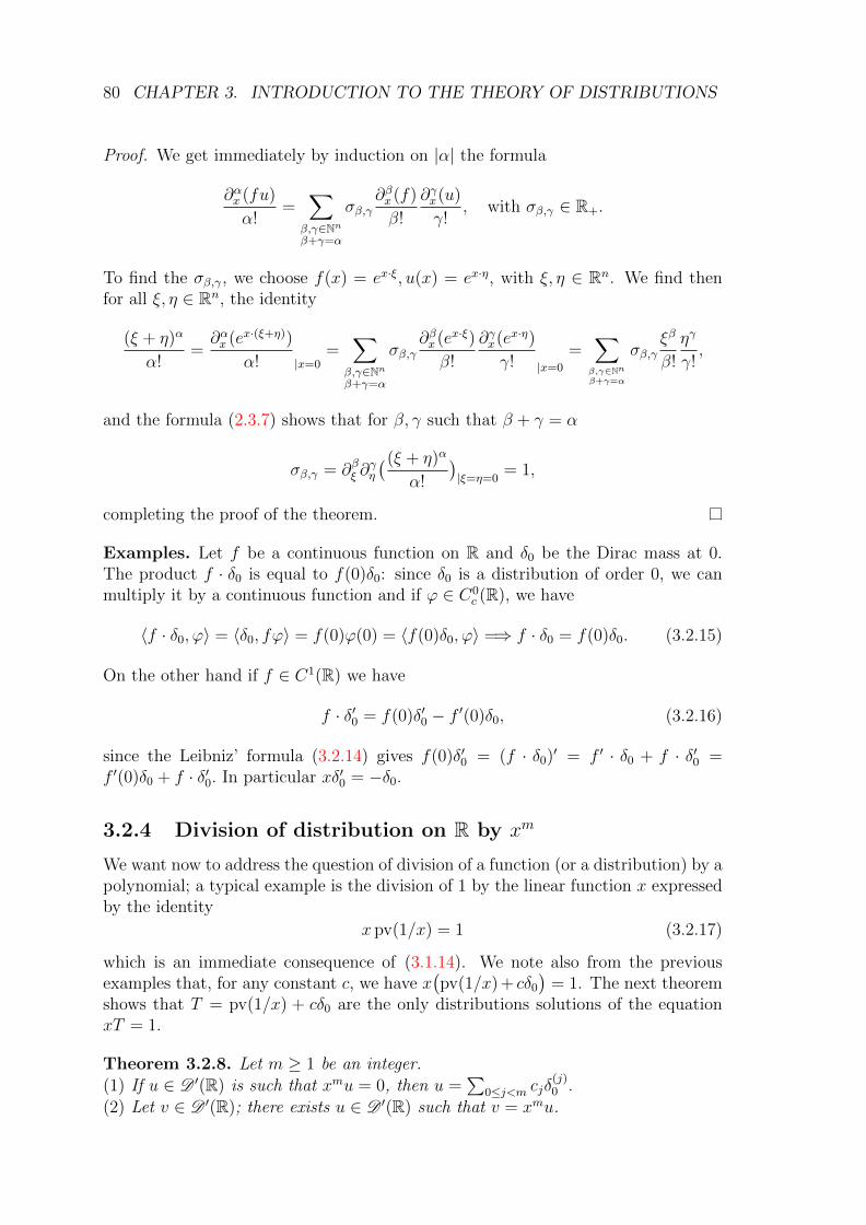
80 CHAPTER 3. INTRODUCTION TO THE THEORY OF DISTRIBUTIONS
Proof. We get immediately by induction on |α| the formula
∂αx (fu)
α!=∑
β,γ∈Nnβ+γ=α
σβ,γ∂βx (f)
β!
∂γx(u)
γ!, with σβ,γ ∈ R+.
To find the σβ,γ, we choose f(x) = ex·ξ, u(x) = ex·η, with ξ, η ∈ Rn. We find thenfor all ξ, η ∈ Rn, the identity
(ξ + η)α
α!=∂αx (ex·(ξ+η))
α! |x=0=∑
β,γ∈Nnβ+γ=α
σβ,γ∂βx (ex·ξ)
β!
∂γx(ex·η)
γ! |x=0
=∑β,γ∈Nnβ+γ=α
σβ,γξβ
β!
ηγ
γ!,
and the formula (2.3.7) shows that for β, γ such that β + γ = α
σβ,γ = ∂βξ ∂γη
((ξ + η)α
α!
)|ξ=η=0
= 1,
completing the proof of the theorem.
Examples. Let f be a continuous function on R and δ0 be the Dirac mass at 0.The product f · δ0 is equal to f(0)δ0: since δ0 is a distribution of order 0, we canmultiply it by a continuous function and if ϕ ∈ C0
c (R), we have
〈f · δ0, ϕ〉 = 〈δ0, fϕ〉 = f(0)ϕ(0) = 〈f(0)δ0, ϕ〉 =⇒ f · δ0 = f(0)δ0. (3.2.15)
On the other hand if f ∈ C1(R) we have
f · δ′0 = f(0)δ′0 − f ′(0)δ0, (3.2.16)
since the Leibniz’ formula (3.2.14) gives f(0)δ′0 = (f · δ0)′ = f ′ · δ0 + f · δ′0 =f ′(0)δ0 + f · δ′0. In particular xδ′0 = −δ0.
3.2.4 Division of distribution on R by xm
We want now to address the question of division of a function (or a distribution) by apolynomial; a typical example is the division of 1 by the linear function x expressedby the identity
x pv(1/x) = 1 (3.2.17)
which is an immediate consequence of (3.1.14). We note also from the previousexamples that, for any constant c, we have x
(pv(1/x) + cδ0
)= 1. The next theorem
shows that T = pv(1/x) + cδ0 are the only distributions solutions of the equationxT = 1.
Theorem 3.2.8. Let m ≥ 1 be an integer.(1) If u ∈ D ′(R) is such that xmu = 0, then u =
∑0≤j<m cjδ
(j)0 .
(2) Let v ∈ D ′(R); there exists u ∈ D ′(R) such that v = xmu.
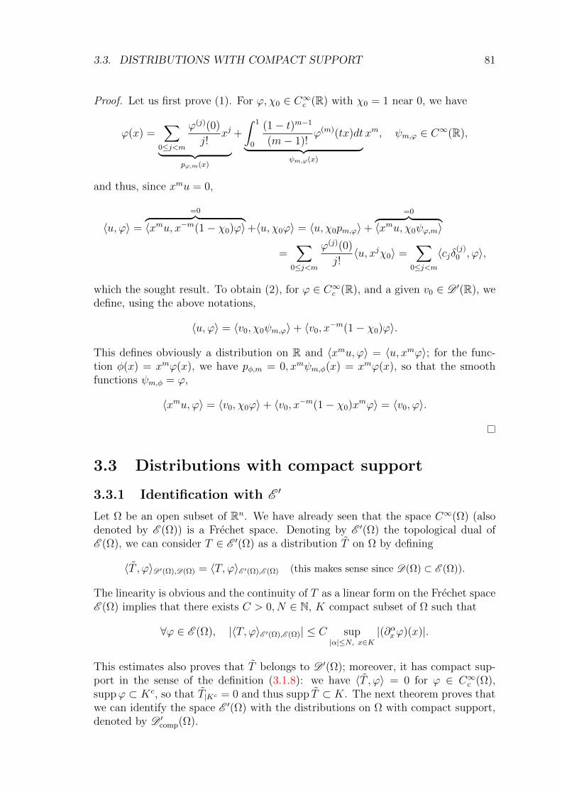
3.3. DISTRIBUTIONS WITH COMPACT SUPPORT 81
Proof. Let us first prove (1). For ϕ, χ0 ∈ C∞c (R) with χ0 = 1 near 0, we have
ϕ(x) =∑
0≤j<m
ϕ(j)(0)
j!xj︸ ︷︷ ︸
pϕ,m(x)
+
∫ 1
0
(1− t)m−1
(m− 1)!ϕ(m)(tx)dt︸ ︷︷ ︸
ψm,ϕ(x)
xm, ψm,ϕ ∈ C∞(R),
and thus, since xmu = 0,
〈u, ϕ〉 =
=0︷ ︸︸ ︷〈xmu, x−m(1− χ0)ϕ〉+〈u, χ0ϕ〉 = 〈u, χ0pm,ϕ〉+
=0︷ ︸︸ ︷〈xmu, χ0ψϕ,m〉
=∑
0≤j<m
ϕ(j)(0)
j!〈u, xjχ0〉 =
∑0≤j<m
〈cjδ(j)0 , ϕ〉,
which the sought result. To obtain (2), for ϕ ∈ C∞c (R), and a given v0 ∈ D ′(R), wedefine, using the above notations,
〈u, ϕ〉 = 〈v0, χ0ψm,ϕ〉+ 〈v0, x−m(1− χ0)ϕ〉.
This defines obviously a distribution on R and 〈xmu, ϕ〉 = 〈u, xmϕ〉; for the func-tion φ(x) = xmϕ(x), we have pφ,m = 0, xmψm,φ(x) = xmϕ(x), so that the smoothfunctions ψm,φ = ϕ,
〈xmu, ϕ〉 = 〈v0, χ0ϕ〉+ 〈v0, x−m(1− χ0)xmϕ〉 = 〈v0, ϕ〉.
3.3 Distributions with compact support
3.3.1 Identification with E ′
Let Ω be an open subset of Rn. We have already seen that the space C∞(Ω) (alsodenoted by E (Ω)) is a Frechet space. Denoting by E ′(Ω) the topological dual ofE (Ω), we can consider T ∈ E ′(Ω) as a distribution T on Ω by defining
〈T , ϕ〉D ′(Ω),D(Ω) = 〈T, ϕ〉E ′(Ω),E (Ω) (this makes sense since D(Ω) ⊂ E (Ω)).
The linearity is obvious and the continuity of T as a linear form on the Frechet spaceE (Ω) implies that there exists C > 0, N ∈ N, K compact subset of Ω such that
∀ϕ ∈ E (Ω), |〈T, ϕ〉E ′(Ω),E (Ω)| ≤ C sup|α|≤N, x∈K
|(∂αxϕ)(x)|.
This estimates also proves that T belongs to D ′(Ω); moreover, it has compact sup-port in the sense of the definition (3.1.8): we have 〈T , ϕ〉 = 0 for ϕ ∈ C∞c (Ω),suppϕ ⊂ Kc, so that T|Kc = 0 and thus supp T ⊂ K. The next theorem proves thatwe can identify the space E ′(Ω) with the distributions on Ω with compact support,denoted by D ′comp(Ω).
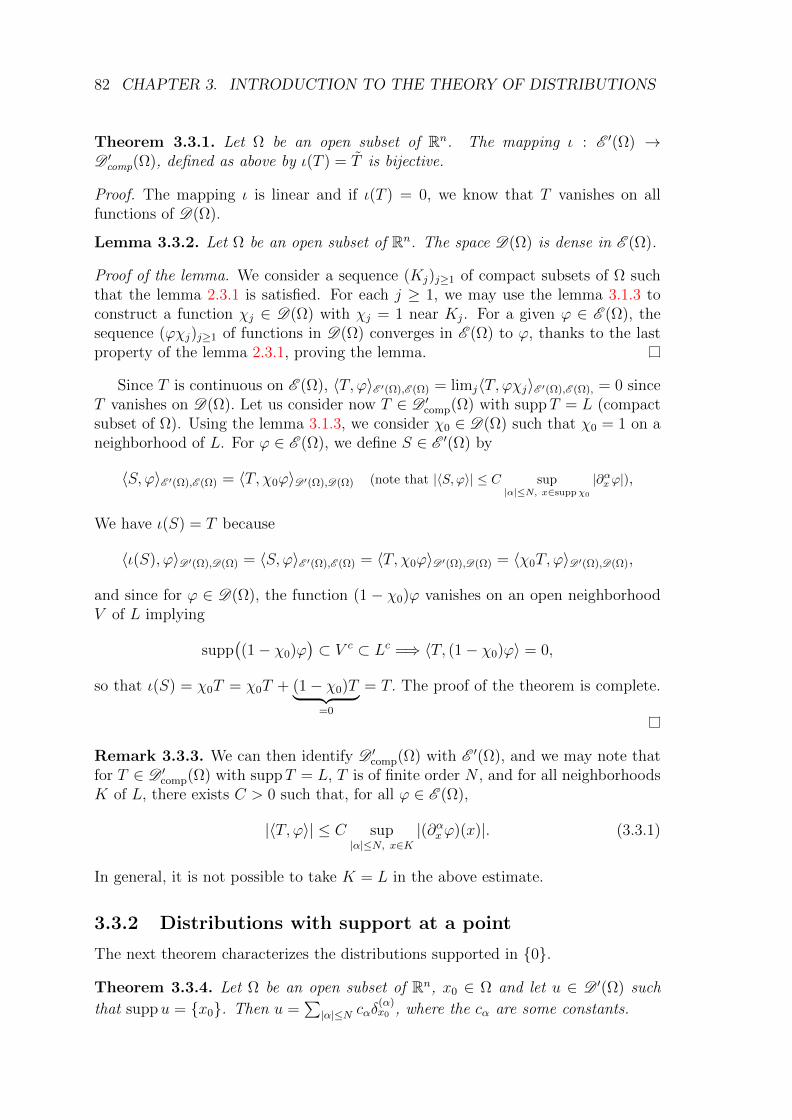
82 CHAPTER 3. INTRODUCTION TO THE THEORY OF DISTRIBUTIONS
Theorem 3.3.1. Let Ω be an open subset of Rn. The mapping ι : E ′(Ω) →D ′comp(Ω), defined as above by ι(T ) = T is bijective.
Proof. The mapping ι is linear and if ι(T ) = 0, we know that T vanishes on allfunctions of D(Ω).
Lemma 3.3.2. Let Ω be an open subset of Rn. The space D(Ω) is dense in E (Ω).
Proof of the lemma. We consider a sequence (Kj)j≥1 of compact subsets of Ω suchthat the lemma 2.3.1 is satisfied. For each j ≥ 1, we may use the lemma 3.1.3 toconstruct a function χj ∈ D(Ω) with χj = 1 near Kj. For a given ϕ ∈ E (Ω), thesequence (ϕχj)j≥1 of functions in D(Ω) converges in E (Ω) to ϕ, thanks to the lastproperty of the lemma 2.3.1, proving the lemma.
Since T is continuous on E (Ω), 〈T, ϕ〉E ′(Ω),E (Ω) = limj〈T, ϕχj〉E ′(Ω),E (Ω), = 0 sinceT vanishes on D(Ω). Let us consider now T ∈ D ′comp(Ω) with suppT = L (compactsubset of Ω). Using the lemma 3.1.3, we consider χ0 ∈ D(Ω) such that χ0 = 1 on aneighborhood of L. For ϕ ∈ E (Ω), we define S ∈ E ′(Ω) by
〈S, ϕ〉E ′(Ω),E (Ω) = 〈T, χ0ϕ〉D ′(Ω),D(Ω) (note that |〈S, ϕ〉| ≤ C sup|α|≤N, x∈suppχ0
|∂αxϕ|),
We have ι(S) = T because
〈ι(S), ϕ〉D ′(Ω),D(Ω) = 〈S, ϕ〉E ′(Ω),E (Ω) = 〈T, χ0ϕ〉D ′(Ω),D(Ω) = 〈χ0T, ϕ〉D ′(Ω),D(Ω),
and since for ϕ ∈ D(Ω), the function (1 − χ0)ϕ vanishes on an open neighborhoodV of L implying
supp((1− χ0)ϕ
)⊂ V c ⊂ Lc =⇒ 〈T, (1− χ0)ϕ〉 = 0,
so that ι(S) = χ0T = χ0T + (1− χ0)T︸ ︷︷ ︸=0
= T. The proof of the theorem is complete.
Remark 3.3.3. We can then identify D ′comp(Ω) with E ′(Ω), and we may note thatfor T ∈ D ′comp(Ω) with suppT = L, T is of finite order N , and for all neighborhoodsK of L, there exists C > 0 such that, for all ϕ ∈ E (Ω),
|〈T, ϕ〉| ≤ C sup|α|≤N, x∈K
|(∂αxϕ)(x)|. (3.3.1)
In general, it is not possible to take K = L in the above estimate.
3.3.2 Distributions with support at a point
The next theorem characterizes the distributions supported in 0.
Theorem 3.3.4. Let Ω be an open subset of Rn, x0 ∈ Ω and let u ∈ D ′(Ω) such
that suppu = x0. Then u =∑|α|≤N cαδ
(α)x0 , where the cα are some constants.
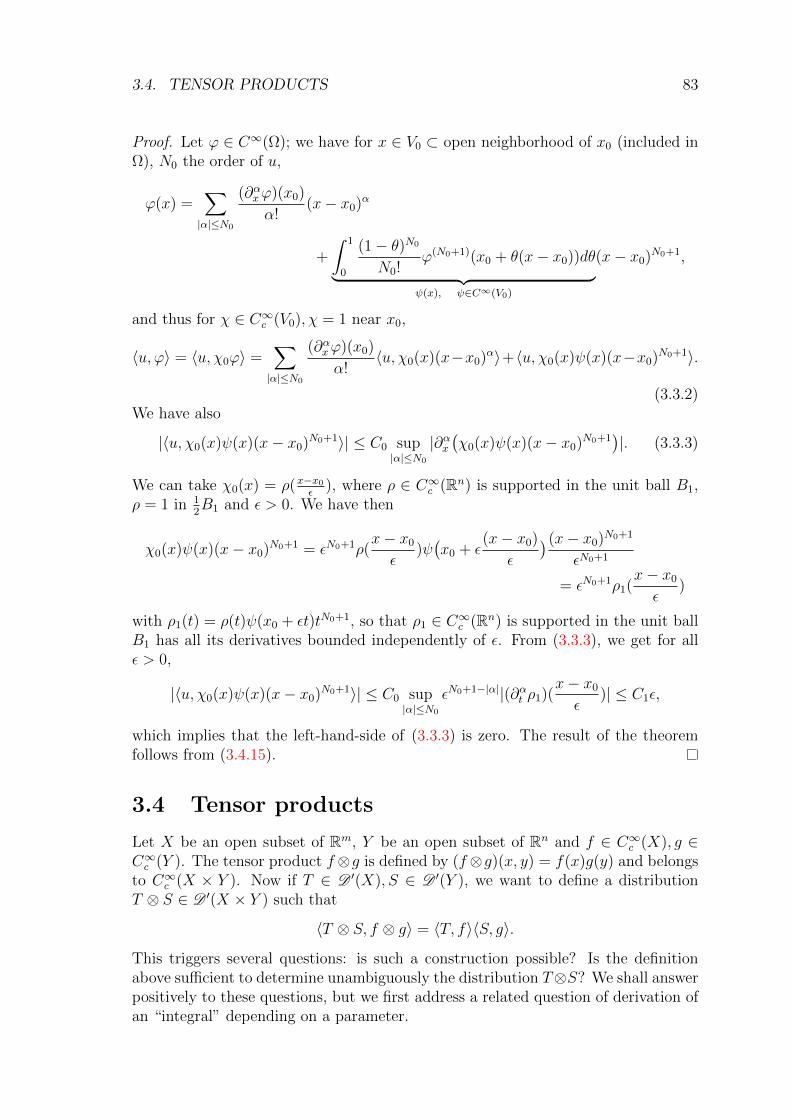
3.4. TENSOR PRODUCTS 83
Proof. Let ϕ ∈ C∞(Ω); we have for x ∈ V0 ⊂ open neighborhood of x0 (included inΩ), N0 the order of u,
ϕ(x) =∑|α|≤N0
(∂αxϕ)(x0)
α!(x− x0)α
+
∫ 1
0
(1− θ)N0
N0!ϕ(N0+1)(x0 + θ(x− x0))dθ︸ ︷︷ ︸ψ(x), ψ∈C∞(V0)
(x− x0)N0+1,
and thus for χ ∈ C∞c (V0), χ = 1 near x0,
〈u, ϕ〉 = 〈u, χ0ϕ〉 =∑|α|≤N0
(∂αxϕ)(x0)
α!〈u, χ0(x)(x−x0)α〉+〈u, χ0(x)ψ(x)(x−x0)N0+1〉.
(3.3.2)We have also
|〈u, χ0(x)ψ(x)(x− x0)N0+1〉| ≤ C0 sup|α|≤N0
|∂αx(χ0(x)ψ(x)(x− x0)N0+1
)|. (3.3.3)
We can take χ0(x) = ρ(x−x0ε
), where ρ ∈ C∞c (Rn) is supported in the unit ball B1,ρ = 1 in 1
2B1 and ε > 0. We have then
χ0(x)ψ(x)(x− x0)N0+1 = εN0+1ρ(x− x0
ε)ψ(x0 + ε
(x− x0)
ε
)(x− x0)N0+1
εN0+1
= εN0+1ρ1(x− x0
ε)
with ρ1(t) = ρ(t)ψ(x0 + εt)tN0+1, so that ρ1 ∈ C∞c (Rn) is supported in the unit ballB1 has all its derivatives bounded independently of ε. From (3.3.3), we get for allε > 0,
|〈u, χ0(x)ψ(x)(x− x0)N0+1〉| ≤ C0 sup|α|≤N0
εN0+1−|α||(∂αt ρ1)(x− x0
ε)| ≤ C1ε,
which implies that the left-hand-side of (3.3.3) is zero. The result of the theoremfollows from (3.4.15).
3.4 Tensor products
Let X be an open subset of Rm, Y be an open subset of Rn and f ∈ C∞c (X), g ∈C∞c (Y ). The tensor product f⊗g is defined by (f⊗g)(x, y) = f(x)g(y) and belongsto C∞c (X × Y ). Now if T ∈ D ′(X), S ∈ D ′(Y ), we want to define a distributionT ⊗ S ∈ D ′(X × Y ) such that
〈T ⊗ S, f ⊗ g〉 = 〈T, f〉〈S, g〉.
This triggers several questions: is such a construction possible? Is the definitionabove sufficient to determine unambiguously the distribution T⊗S? We shall answerpositively to these questions, but we first address a related question of derivation ofan “integral” depending on a parameter.
84 CHAPTER 3. INTRODUCTION TO THE THEORY OF DISTRIBUTIONS
3.4.1 Differentiation of a duality product
Theorem 3.4.1. Let Ω be an open subset of Rn, u ∈ D ′(Ω), U an open subset ofRm and φ ∈ C∞(Ω× U) such that
∀t ∈ U,∃Vt ∈ Vt,∃Kt compact subset of Ω, ∀s ∈ Vt, suppφ(·, s) ⊂ Kt. (3.4.1)
Then the function f defined on U by f(t) = 〈u, φ(·, t)〉 makes sense and belongs toC∞(U). Moreover we have for all α ∈ Nm, (∂αt f)(t) = 〈u, (∂αt φ)(·, t)〉.
Proof. The function f makes sense since for all t ∈ U , the function φ(·, t) belongsto C∞c (Ω). Let t0 ∈ U and B0 be a closed ball with center t0 and positive radius r0
included in Vt0 given by (3.4.1). For |h| ≤ r0, we have
f(t0 + h)− f(t0) = 〈u, φ(·, t0 + h)− φ(·, t0)︸ ︷︷ ︸supported in Kt0 ,
〉
and using Taylor’s formula with integral remainder, we get
f(t0 + h)− f(t0) = 〈u, (∂tφ)(·, t0)〉h+ 〈u,∫ 1
0
(1− θ)
support in Kt0︷ ︸︸ ︷∂2sφ(·, t0 + θh) dθ〉h2︸ ︷︷ ︸r(t0,h)
.
We have, since Kt0 ×B0 is a compact subset of Ω× U ,
|r(t0, h)| ≤ |h|2C0 supx∈Kt0 ,|α|≤N0
∫ 1
0
(1− θ)|(∂αx∂2sφ) (x, t0 + θ0h)︸ ︷︷ ︸
∈Kt0×B0
|dθ ≤ C1|h|2,
proving the differentiability of f on U along with df(t) = 〈u, ∂tφ(·, t)〉. Inductively,we get that f is smooth and the result of the theorem.
Corollary 3.4.2. Let X, Y be open subsets of Rn,Rm, φ ∈ C∞(X × Y ) and u ∈D ′(X).(1) If φ is compactly supported in X×Y , the function ψ defined by ψ(y) = 〈u, φ(·, y)〉belongs to C∞c (Y ).(2) If u ∈ E ′(X), the function ψ defined by ψ(y) = 〈u, φ(·, y)〉 belongs to C∞(Y ).
Proof. To prove (1), we need only to verify (3.4.1): we have indeed for all y ∈ Y
suppφ(·, y) ⊂ projX(suppφ) which is a compact subset of X,
which implies that ψ ∈ C∞(Y ); moreover the function φ(·, y) = 0 on the open subsetof Y ,
(projY (suppφ)
)c, and thus suppψ ⊂ projY (suppφ) which is a compact subset
of Y . To obtain (2), we consider χ ∈ C∞c (X) equal to 1 near the compact supportof u. We have then u = χu and consequently,
〈u, φ(·, y)〉 = 〈u, φ(·, y)χ(·)〉.
The function Φ(x, y) = φ(x, y)χ(x) is smooth on X × Y and supp Φ(·, y) ⊂ suppχso that we can apply the theorem 3.4.1 whose assumptions are satisfied.
3.4. TENSOR PRODUCTS 85
3.4.2 Pull-back by the affine group
Let us now recall the definition of the affine group of Rn: it is the group of mappingsfrom Rn into itself of the form x 7→ Ax + t = θA,t(x) where A ∈ Gl(n,R)(n ×n invertible matrices) and t ∈ Rn. When A is the identity, ΘId,t is simply thetranslation of vector t; we have also θ−1
A,t = ΘA−1,−A−1t. If u belongs to L1loc(Rn) and
ΘA,t is in the affine group of Rn, we can define the pull-back of u by the map Θ bythe identity
Θ∗A,tu = u ΘA,t, so that (Θ∗A,tu)(x) = u(Ax+ t). (3.4.2)
As a result for ϕ ∈ C0c (Rn), we find
〈Θ∗A,tu, ϕ〉 =
∫Rnu(Ax+ t)ϕ(x)dx =
∫Rnu(y)ϕ(A−1y − A−1t)| detA|−1dy. (3.4.3)
We want to use that formula to define the pull-back of a distribution on Rn by anaffine transformation.
Definition 3.4.3. Let A ∈ Gl(n,R), t ∈ Rn, ΘA,t the affine transformation definedabove and let u ∈ D ′(Rn). We define the distribution Θ∗A,tu by the identity
〈Θ∗A,tu, ϕ〉 = 〈u, ϕ Θ−1A,t〉| detA|−1. (3.4.4)
Remark 3.4.4. (1) Note that this defines a distribution on Rn, since the mappingϕ 7→ ϕ Θ−1
A,t is an isomorphism of D(Rn). Moreover, if u ∈ L1loc(Rn), the previous
definition ensures that Θ∗A,tu = u ΘA,t, thanks to the lemma 3.1.7.(2) The mapping u 7→ Θ∗A,tu is sequentially continuous from D ′(Rn) into itself.(3) A distribution u on Rn is even (resp. odd) if Θ∗− Id,0u = u (resp. −u). Using thenotation
u = Θ∗− Id,0u (for a function u, u(x) = u(−x)), (3.4.5)
u is even means u = u, odd means u = −u.
3.4.3 Homogeneous distributions
Definition 3.4.5. Let u ∈ D ′(Rn) and λ ∈ C. The distribution u is said to behomogeneous with degree λ if for all t > 0, u(t·) = tλu(·) (here u(t·) = θ∗t Id,0u).
Proposition 3.4.6. Let u ∈ D ′(Rn) and λ ∈ C. The distribution u is homogeneousof degree λ if and only if the Euler equation is satisfied, namely∑
1≤j≤n
xj∂xju = λu. (3.4.6)
Proof. A distribution u on Rn is homogeneous of degree λ means:
∀ϕ ∈ C∞c (Rn),∀t > 0, 〈u(y), ϕ(y/t)t−n〉 = tλ〈u(x), ϕ(x)〉,
which is equivalent to ∀ϕ ∈ C∞c (Rn),∀s > 0, 〈u(y), ϕ(sy)sn+λ〉 = 〈u(x), ϕ(x)〉, alsoequivalent to
∀ϕ ∈ C∞c (Rn),d
ds
(〈u(y), ϕ(sy)sn+λ〉
)= 0 on s > 0. (3.4.7)
86 CHAPTER 3. INTRODUCTION TO THE THEORY OF DISTRIBUTIONS
Note that the differentiability property is due to the theorem 3.4.1 and that
〈u(y), ϕ(sy)sn+λ〉 = 〈u(x), ϕ(x)〉 at s = 1.
As a consequence, applying the theorem 3.4.1, we get that the homogeneity of degreeλ of u is equivalent to
∀s > 0, 〈u(y), sn+λ−1((n+ λ)ϕ(sy) +
∑1≤j≤n
(∂jϕ)(sy)syj)〉 = 0,
also equivalent to 0 = 〈u(y), (n+ λ+∑
1≤j≤n yj∂j)(ϕ(sy)
)〉 and by the definition of
the differentiation of a distribution, it is equivalent to (n+λ)u−∑
1≤j≤n ∂j(yju) = 0,which is (3.4.6) by the Leibniz rule (3.2.14).
Remark 3.4.7. (1) The Dirac mass at 0 in Rn is homogeneous of degree −n: wehave for t > 0
〈δ0(tx), ϕ(x)〉 = 〈δ0(y), ϕ(y/t)t−n〉 = t−nϕ(0) = t−n〈δ0, ϕ〉.
(2) If T is an homogeneous distribution of degree λ, then ∂αxT is also homogeneouswith degree λ− |α|: taking the derivative of the Euler equation (3.4.6), we get
∂xku+∑
1≤j≤k
xj∂xj∂xku− λ∂xku = 0,
proving that ∂xku is homogeneous of degree λ− 1 and the result by iteration.(3) It follows immediately from the definition (3.1.14) that the distribution pv( 1
x) is
homogeneous of degree −1. The same is true for the distributions 1x±i0 as it is clear
from (3.2.9)and (3.2.10).(4) For λ ∈ C with Reλ > −1 we define the L1
loc(R) functions
xλ+ =
xλ if x > 0,
0 if x ≤ 0.,χλ+ =
xλ+Γ(λ+ 1)
. (3.4.8)
The distributions χλ+ and xλ+ are homogeneous of degree λ and by an analytic con-tinuation argument, we can prove that χλ+ may be defined for any λ ∈ C, is anhomogeneous distribution of degree λ and satisfies
χλ+ = (d
dx)k(χλ+k
+ ), χ−k+ = δ(k−1)0 , k ∈ N∗.
Lemma 3.4.8. Let (uj)1≤j≤m be non-zero homogeneous distributions on Rn withdistinct degrees (λj)1≤j≤m (j 6= k implies λj 6= λk). Then they are independent inthe complex vector space D ′(Rn).
Proof. We assume thatm ≥ 2 and that there exists some complex numbers (cj)1≤j≤msuch that
∑1≤j≤m cjuj = 0. Then applying the operator E =
∑1≤j≤m xj∂xj , we get
for all k ∈ N,
0 =∑
1≤j≤m
cjEk(uj) =∑
1≤j≤m
cjλkjuj.
3.4. TENSOR PRODUCTS 87
We consider now the Vandermonde matrix m×m
Vm =
1 1 . . . 1λ1 λ2 . . . λm
. . . .λm−1
1 λm−12 . . . λm−1
m
, detVm =∏
1≤j<k≤m
(λk − λj) 6= 0.
We note that for ϕ ∈ C∞c (Rn), and X ∈ Cm given by
X =
c1〈u1, ϕ〉c2〈u2, ϕ〉. . . . . . . . .cm〈um, ϕ〉
,
we have VmX = 0, so that X = 0, i.e. ∀j,∀ϕ ∈ C∞c (Rn), cj〈uj, ϕ〉 = 0, i.e. cjuj = 0and since uj is not the zero distribution, we get the sought conclusion cj = 0 for allj.
3.4.4 Tensor products of distributions
We begin with a lemma.
Lemma 3.4.9. Let φ ∈ C∞c (]0, 1[n); one can find a sequence of functions in
Vect(⊗nC∞c (]0, 1[) (the vector space generated by the tensor products)
converging to φ in C∞c (]0, 1[n) in the sense of the definition 3.1.9.
Proof. We define for k ∈ Zn, φ(k) =∫e−2iπx·kφ(x)dx, and we note that, with
∆ =∑
1≤j≤n ∂2xj
, m ∈ N,
φ(k) = (1 + |k|2)−m∫
(1− 1
4π2∆)m
(e−2iπx·k)φ(x)dx
= (1 + |k|2)−m∫e−2iπx·k((1− 1
4π2∆)mφ
)(x)dx
so that|φ(k)| ≤ (1 + |k|2)−mCm max
|α|≤2m‖∂αxφ‖L∞ . (3.4.9)
As a result the series Φ(x) =∑
k∈Zn φ(k)e2iπx·k converges and is a smooth function,periodic with periods Zn: we need only to check that
∑k∈Zn(1 + |k|)−n−1 < +∞.3
Moreover,for x ∈ [0, 1]n, Φ(x) = φ(x). (3.4.10)
3In fact, with Qk = k + (0, 1)n we have, replacing the Euclidean norm |k| by the (equivalent)sup-norm ‖k‖ = max1≤j≤k |kj |, we have for x ∈ Qk, kj < xj < kj + 1 and thus
‖x‖ = max |xj | ≤ 1 + ‖k‖ =⇒ 1 + ‖x‖ ≤ 2 + ‖k‖
and∑k∈Zn(2 + ‖k‖)−n−1 ≤
∫ ∑k∈Zn 1Qk(x)(1 + ‖x‖)−n−1dx =
∫(1 + ‖x‖)−n−1dx < +∞.
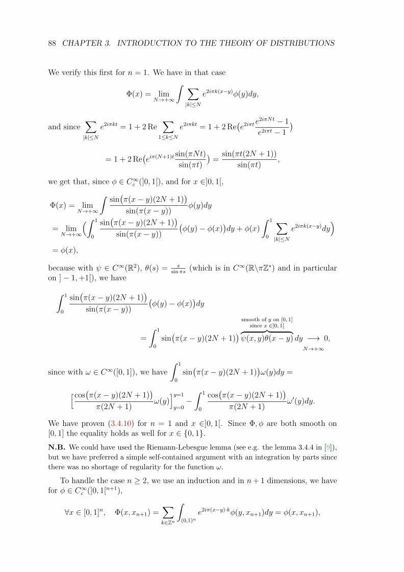
88 CHAPTER 3. INTRODUCTION TO THE THEORY OF DISTRIBUTIONS
We verify this first for n = 1. We have in that case
Φ(x) = limN→+∞
∫ ∑|k|≤N
e2iπk(x−y)φ(y)dy,
and since∑|k|≤N
e2iπkt = 1 + 2 Re∑
1≤k≤N
e2iπkt = 1 + 2 Re(e2iπt e
2iπNt − 1
e2iπt − 1
)
= 1 + 2 Re(eiπ(N+1)t sin(πNt)
sin(πt)
)=
sin(πt(2N + 1))
sin(πt),
we get that, since φ ∈ C∞c (]0, 1[), and for x ∈]0, 1[,
Φ(x) = limN→+∞
∫sin(π(x− y)(2N + 1)
)sin(π(x− y))
φ(y)dy
= limN→+∞
(∫ 1
0
sin(π(x− y)(2N + 1)
)sin(π(x− y))
(φ(y)− φ(x)
)dy + φ(x)
∫ 1
0
∑|k|≤N
e2iπk(x−y)dy)
= φ(x),
because with ψ ∈ C∞(R2), θ(s) = ssinπs
(which is in C∞(R\πZ∗) and in particularon ]− 1,+1[), we have∫ 1
0
sin(π(x− y)(2N + 1)
)sin(π(x− y))
(φ(y)− φ(x)
)dy
=
∫ 1
0
sin(π(x− y)(2N + 1)
) smooth of y on [0, 1]since x ∈]0, 1[︷ ︸︸ ︷
ψ(x, y)θ(x− y) dy −→N→+∞
0,
since with ω ∈ C∞([0, 1]), we have
∫ 1
0
sin(π(x− y)(2N + 1)
)ω(y)dy =
[cos(π(x− y)(2N + 1)
)π(2N + 1)
ω(y)]y=1
y=0−∫ 1
0
cos(π(x− y)(2N + 1)
)π(2N + 1)
ω′(y)dy.
We have proven (3.4.10) for n = 1 and x ∈]0, 1[. Since Φ, φ are both smooth on[0, 1] the equality holds as well for x ∈ 0, 1.
N.B. We could have used the Riemann-Lebesgue lemma (see e.g. the lemma 3.4.4 in [9]),
but we have preferred a simple self-contained argument with an integration by parts since
there was no shortage of regularity for the function ω.
To handle the case n ≥ 2, we use an induction and in n+ 1 dimensions, we havefor φ ∈ C∞c (]0, 1[n+1),
∀x ∈ [0, 1]n, Φ(x, xn+1) =∑k∈Zn
∫(0,1)n
e2iπ(x−y)·kφ(y, xn+1)dy = φ(x, xn+1),
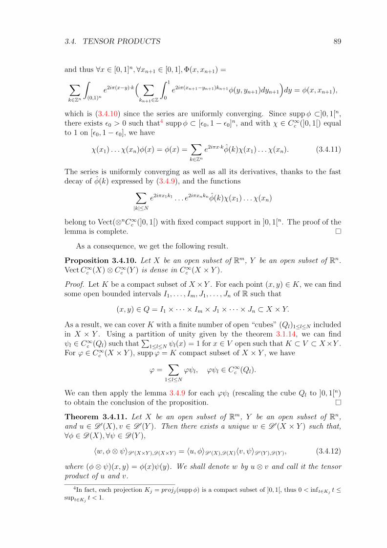
3.4. TENSOR PRODUCTS 89
and thus ∀x ∈ [0, 1]n,∀xn+1 ∈ [0, 1],Φ(x, xn+1) =∑k∈Zn
∫(0,1)n
e2iπ(x−y)·k( ∑kn+1∈Z
∫ 1
0
e2iπ(xn+1−yn+1)kn+1φ(y, yn+1)dyn+1
)dy = φ(x, xn+1),
which is (3.4.10) since the series are uniformly converging. Since suppφ ⊂]0, 1[n,there exists ε0 > 0 such that4 suppφ ⊂ [ε0, 1 − ε0]n, and with χ ∈ C∞c (]0, 1[) equalto 1 on [ε0, 1− ε0], we have
χ(x1) . . . χ(xn)φ(x) = φ(x) =∑k∈Zn
e2iπx·kφ(k)χ(x1) . . . χ(xn). (3.4.11)
The series is uniformly converging as well as all its derivatives, thanks to the fastdecay of φ(k) expressed by (3.4.9), and the functions∑
|k|≤N
e2iπx1k1 . . . e2iπxnknφ(k)χ(x1) . . . χ(xn)
belong to Vect(⊗nC∞c (]0, 1[) with fixed compact support in ]0, 1[n. The proof of thelemma is complete.
As a consequence, we get the following result.
Proposition 3.4.10. Let X be an open subset of Rm, Y be an open subset of Rn.VectC∞c (X)⊗ C∞c (Y ) is dense in C∞c (X × Y ).
Proof. Let K be a compact subset of X×Y . For each point (x, y) ∈ K, we can findsome open bounded intervals I1, . . . , Im, J1, . . . , Jn of R such that
(x, y) ∈ Q = I1 × · · · × Im × J1 × · · · × Jn ⊂ X × Y.
As a result, we can cover K with a finite number of open “cubes” (Ql)1≤l≤N includedin X × Y . Using a partition of unity given by the theorem 3.1.14, we can findψl ∈ C∞c (Ql) such that
∑1≤l≤N ψl(x) = 1 for x ∈ V open such that K ⊂ V ⊂ X×Y .
For ϕ ∈ C∞c (X × Y ), suppϕ = K compact subset of X × Y , we have
ϕ =∑
1≤l≤N
ϕψl, ϕψl ∈ C∞c (Ql).
We can then apply the lemma 3.4.9 for each ϕψl (rescaling the cube Ql to ]0, 1[n)to obtain the conclusion of the proposition.
Theorem 3.4.11. Let X be an open subset of Rm, Y be an open subset of Rn,and u ∈ D ′(X), v ∈ D ′(Y ). Then there exists a unique w ∈ D ′(X × Y ) such that,∀φ ∈ D(X),∀ψ ∈ D(Y ),
〈w, φ⊗ ψ〉D ′(X×Y ),D(X×Y ) = 〈u, φ〉D ′(X),D(X)〈v, ψ〉D ′(Y ),D(Y ), (3.4.12)
where (φ⊗ ψ)(x, y) = φ(x)ψ(y). We shall denote w by u⊗ v and call it the tensorproduct of u and v.
4In fact, each projection Kj = projj(suppφ) is a compact subset of ]0, 1[, thus 0 < inft∈Kj t ≤supt∈Kj t < 1.
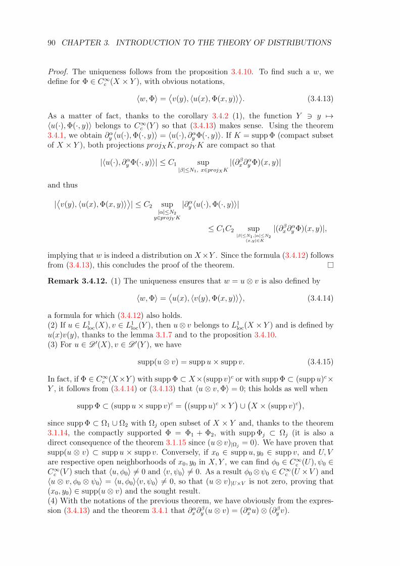
90 CHAPTER 3. INTRODUCTION TO THE THEORY OF DISTRIBUTIONS
Proof. The uniqueness follows from the proposition 3.4.10. To find such a w, wedefine for Φ ∈ C∞c (X × Y ), with obvious notations,
〈w,Φ〉 =⟨v(y), 〈u(x),Φ(x, y)〉
⟩. (3.4.13)
As a matter of fact, thanks to the corollary 3.4.2 (1), the function Y 3 y 7→〈u(·),Φ(·, y)〉 belongs to C∞c (Y ) so that (3.4.13) makes sense. Using the theorem3.4.1, we obtain ∂αy 〈u(·),Φ(·, y)〉 = 〈u(·), ∂αy Φ(·, y)〉. If K = supp Φ (compact subsetof X × Y ), both projections projXK, projYK are compact so that
|〈u(·), ∂αy Φ(·, y)〉| ≤ C1 sup|β|≤N1, x∈projXK
|(∂βx∂αy Φ)(x, y)|
and thus
|⟨v(y), 〈u(x),Φ(x, y)〉
⟩| ≤ C2 sup
|α|≤N2y∈projYK
|∂αy 〈u(·),Φ(·, y)〉|
≤ C1C2 sup|β|≤N1,|α|≤N2
(x,y)∈K
|(∂βx∂αy Φ)(x, y)|,
implying that w is indeed a distribution on X×Y . Since the formula (3.4.12) followsfrom (3.4.13), this concludes the proof of the theorem.
Remark 3.4.12. (1) The uniqueness ensures that w = u⊗ v is also defined by
〈w,Φ〉 =⟨u(x), 〈v(y),Φ(x, y)〉
⟩, (3.4.14)
a formula for which (3.4.12) also holds.(2) If u ∈ L1
loc(X), v ∈ L1loc(Y ), then u⊗ v belongs to L1
loc(X × Y ) and is defined byu(x)v(y), thanks to the lemma 3.1.7 and to the proposition 3.4.10.(3) For u ∈ D ′(X), v ∈ D ′(Y ), we have
supp(u⊗ v) = suppu× supp v. (3.4.15)
In fact, if Φ ∈ C∞c (X×Y ) with supp Φ ⊂ X×(supp v)c or with supp Φ ⊂ (suppu)c×Y , it follows from (3.4.14) or (3.4.13) that 〈u⊗ v,Φ〉 = 0; this holds as well when
supp Φ ⊂ (suppu× supp v)c =((suppu)c × Y
)∪(X × (supp v)c
),
since supp Φ ⊂ Ω1 ∪ Ω2 with Ωj open subset of X × Y and, thanks to the theorem3.1.14, the compactly supported Φ = Φ1 + Φ2, with supp Φj ⊂ Ωj (it is also adirect consequence of the theorem 3.1.15 since (u⊗ v)|Ωj = 0). We have proven thatsupp(u ⊗ v) ⊂ suppu × supp v. Conversely, if x0 ∈ suppu, y0 ∈ supp v, and U, Vare respective open neighborhoods of x0, y0 in X, Y , we can find φ0 ∈ C∞c (U), ψ0 ∈C∞c (V ) such that 〈u, φ0〉 6= 0 and 〈v, ψ0〉 6= 0. As a result φ0⊗ψ0 ∈ C∞c (U ×V ) and〈u ⊗ v, φ0 ⊗ ψ0〉 = 〈u, φ0〉〈v, ψ0〉 6= 0, so that (u ⊗ v)|U×V is not zero, proving that(x0, y0) ∈ supp(u⊗ v) and the sought result.(4) With the notations of the previous theorem, we have obviously from the expres-sion (3.4.13) and the theorem 3.4.1 that ∂αx∂
βy (u⊗ v) = (∂αxu)⊗ (∂βy v).
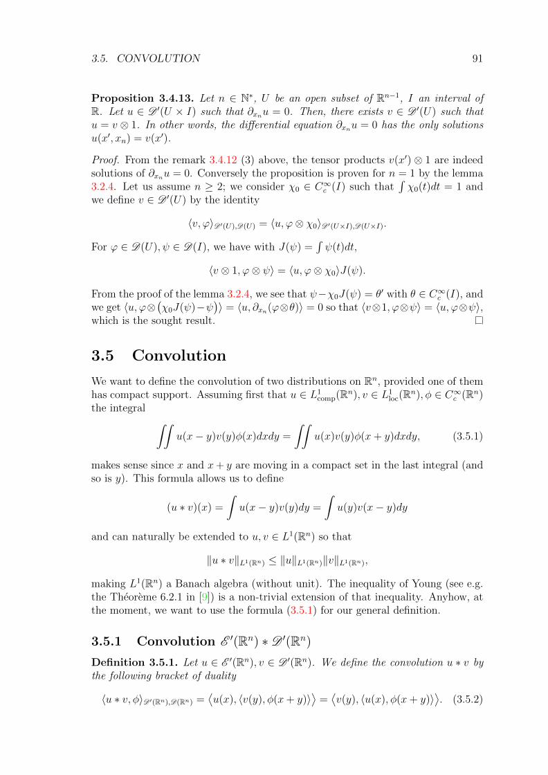
3.5. CONVOLUTION 91
Proposition 3.4.13. Let n ∈ N∗, U be an open subset of Rn−1, I an interval ofR. Let u ∈ D ′(U × I) such that ∂xnu = 0. Then, there exists v ∈ D ′(U) such thatu = v ⊗ 1. In other words, the differential equation ∂xnu = 0 has the only solutionsu(x′, xn) = v(x′).
Proof. From the remark 3.4.12 (3) above, the tensor products v(x′) ⊗ 1 are indeedsolutions of ∂xnu = 0. Conversely the proposition is proven for n = 1 by the lemma3.2.4. Let us assume n ≥ 2; we consider χ0 ∈ C∞c (I) such that
∫χ0(t)dt = 1 and
we define v ∈ D ′(U) by the identity
〈v, ϕ〉D ′(U),D(U) = 〈u, ϕ⊗ χ0〉D ′(U×I),D(U×I).
For ϕ ∈ D(U), ψ ∈ D(I), we have with J(ψ) =∫ψ(t)dt,
〈v ⊗ 1, ϕ⊗ ψ〉 = 〈u, ϕ⊗ χ0〉J(ψ).
From the proof of the lemma 3.2.4, we see that ψ−χ0J(ψ) = θ′ with θ ∈ C∞c (I), andwe get 〈u, ϕ⊗
(χ0J(ψ)−ψ
)〉 = 〈u, ∂xn(ϕ⊗θ)〉 = 0 so that 〈v⊗1, ϕ⊗ψ〉 = 〈u, ϕ⊗ψ〉,
which is the sought result.
3.5 Convolution
We want to define the convolution of two distributions on Rn, provided one of themhas compact support. Assuming first that u ∈ L1
comp(Rn), v ∈ L1loc(Rn), φ ∈ C∞c (Rn)
the integral ∫∫u(x− y)v(y)φ(x)dxdy =
∫∫u(x)v(y)φ(x+ y)dxdy, (3.5.1)
makes sense since x and x+ y are moving in a compact set in the last integral (andso is y). This formula allows us to define
(u ∗ v)(x) =
∫u(x− y)v(y)dy =
∫u(y)v(x− y)dy
and can naturally be extended to u, v ∈ L1(Rn) so that
‖u ∗ v‖L1(Rn) ≤ ‖u‖L1(Rn)‖v‖L1(Rn),
making L1(Rn) a Banach algebra (without unit). The inequality of Young (see e.g.the Theoreme 6.2.1 in [9]) is a non-trivial extension of that inequality. Anyhow, atthe moment, we want to use the formula (3.5.1) for our general definition.
3.5.1 Convolution E ′(Rn) ∗D ′(Rn)
Definition 3.5.1. Let u ∈ E ′(Rn), v ∈ D ′(Rn). We define the convolution u ∗ v bythe following bracket of duality
〈u ∗ v, φ〉D ′(Rn),D(Rn) =⟨u(x), 〈v(y), φ(x+ y)〉
⟩=⟨v(y), 〈u(x), φ(x+ y)〉
⟩. (3.5.2)
92 CHAPTER 3. INTRODUCTION TO THE THEORY OF DISTRIBUTIONS
We note that the theorem 3.4.1 shows that the function Rn 3 x 7→ 〈v(y), φ(x+y)〉is C∞ and thus that the first definition makes sense from the corollary 3.4.2 (2). Tocheck the second equality above, we note that with χ ∈ C∞c (Rn) equal to 1 near thesupport of u, we have χu = u and thus from the remark 3.4.12(1) and the formula(3.4.13),⟨u(x), 〈v(y), φ(x+ y)〉
⟩=⟨u(x), 〈v(y), χ(x)φ(x+ y)〉
⟩= 〈u(x)⊗ v(y), χ(x)φ(x+ y)〉,
which is also equal to⟨v(y), 〈u(x), χ(x)φ(x + y)〉
⟩=⟨v(y), 〈u(x), φ(x + y)〉
⟩. This
proves as well that u ∗ v is a distribution on Rn since the mapping C∞c (Rn) 3 φ 7→Φ ∈ C∞c (R2n), with Φ(x, y) = φ(x+ y)χ(x) is continuous.
Remark 3.5.2. We note that whatever is χ ∈ C∞c (Rn) equal to 1 near the supportof u, we have for u ∈ E ′(Rn), v ∈ D ′(Rn),
〈u ∗ v, φ〉 = 〈u(x)⊗ v(y), χ(x)φ(x+ y)〉. (3.5.3)
Proposition 3.5.3. Let u ∈ E ′(Rn), v ∈ D ′(Rn). We have
supp(u ∗ v) ⊂ suppu+ supp v. (3.5.4)
Proof. Note first that suppu+supp v is a closed subset of Rn as the sum of a compactset and a closed set (exercise). Now if φ ∈ C∞c (Rn) with suppφ ⊂ (suppu+supp v)c,then
supp((x, y) 7→ φ(x+ y)
)⊂ (suppu× supp v)c. (3.5.5)
In fact, if (x0, y0) ∈ suppu× supp v, then x0 + y0 ∈ suppu+ supp v ⊂ (suppφ)c, thelatter being open so that there exists U open in V0 with φ(x0 +U + y0 +U) = 0. Asa consequence, the open set (x0 + U)× (y0 + U) ⊂
(supp((x, y) 7→ φ(x + y))
)cand
this implies (x0, y0) ∈(supp((x, y) 7→ φ(x+ y))
)cand proves (3.5.5), so that (3.5.3),
(3.4.15) give the conclusion of the proposition.
Remark 3.5.4. For u, v both in E ′(Rn), the formula (3.5.2) ensures that u∗v = v∗u.
3.5.2 Regularization
Proposition 3.5.5. Let u ∈ D ′(Rn), ρ ∈ C∞c (Rn). Then ρ ∗ u belongs to C∞(Rn).
Proof. We have from the definitions, with χ ∈ C∞c (Rn) equal to 1 near supp ρ,φ ∈ C∞c (Rn),
〈ρ ∗ u, φ〉 = 〈ρ(x)⊗ u(y), χ(x)φ(x+ y)〉 = 〈u(y), 〈ρ(x), χ(x)φ(x+ y)〉〉, (3.5.6)
and we note that 〈ρ(x), χ(x)φ(x + y)〉 =∫ρ(x)φ(x + y)dx =
∫ρ(x− y)φ(x)dx. As
a result, we have
〈ρ ∗ u, φ〉 = 〈u(y),
∫ρ(x− y)φ(x)︸ ︷︷ ︸∈C∞c (R2n)
dx〉 =
∫φ(x)〈u(y), ρ(x− y)〉dx
3.5. CONVOLUTION 93
where the last equality is due to the theorem 3.4.15 which gives also that ψ(x) =〈u(y), ρ(x − y)〉 is C∞; we have proven ρ ∗ u = ψ and the result. We note also theformula following from (3.5.6)
〈ρ ∗ u, φ〉 = 〈u, ρ ∗ φ〉. (3.5.7)
Lemma 3.5.6. Let Ω be an open subset of Rn and T ∈ D ′(Ω). There exists asequence (ψj)j≥1 in D(Ω) such that limj ψj = T in the weak-dual topology sense ofthe definition 3.1.16.
Proof. We consider first a sequence (Kj)j≥1 of compact subsets of Ω as in the lemma2.3.1 and a sequence (χj)j≥1 such that χj ∈ C∞c (intKj+1), χj = 1 near Kj (see thelemma 3.1.3). In the weak-dual topology sense, we have limj χjT = T : let ϕ ∈ D(Ω),K = suppϕ. From the lemma 2.3.1, there exists j such that suppϕ ⊂ Kj andthus ϕχj = ϕ, implying 〈Tχj, ϕ〉 = 〈T, χjϕ〉 = 〈T, ϕ〉. We can also consider thecompactly supported distribution χjT and see it as a distribution on Rn. We takenow a function ρ ∈ C∞c (Rn) such that
∫ρ(x)dx = 1. According to the first example
in the section 3.1.3, we define ρε (it tends to the Dirac mass at 0 in the weak-dualtopology when ε→ 0+). For ϕ ∈ D(Ω), using (3.5.7), we have
〈ρε ∗ (χjT ), ϕ〉 = 〈χjT, ρε ∗ ϕ〉. (3.5.8)
Considering now a decreasing sequence of positive numbers (εj) with limit 0 suchthat
suppχj + εj supp ρ ⊂ int(Kj+1) ⊂ Ω,
and we define Tj = ρεj ∗ χjT. We have from the proposition 3.5.3 that suppTj iscompact included in Ω and also that Tj ∈ C∞ (proposition 3.5.5). Going back to(3.5.8), for a fixed ϕ, we can find j such that suppϕ ⊂ Kj−1 for j ≥ j0, implyingthat
supp(ρεj ∗ ϕ) ⊂ Kj−1 + εj supp ρ ⊂ suppχj−1 + εj−1 supp ρ ⊂ Kj,
implying that χj(ρεj ∗ ϕ) = ρεj ∗ ϕ and 〈ρεj ∗ (χjT ), ϕ〉 = 〈T, ρεj ∗ ϕ〉. The resultfollows from the proposition 3.1.1 (implying limj(ρεj ∗ ϕ) = ϕ in C∞c (Ω)) and the(sequential) continuity of the distribution T .
Proposition 3.5.7. Let u ∈ E ′(Rn), v ∈ D ′(Rn). We have
singsupp(u ∗ v) ⊂ singsuppu+ singsupp v. (3.5.9)
Proof. We can choose χ ∈ C∞c (Rn) equal to 1 near the singsuppu, ψ ∈ C∞ equal to1 near the singular support of v. We have from the proposition 3.5.5
u ∗ v = (χu) ∗ v + (
∈C∞c (Rn)︷ ︸︸ ︷(1− χ)u) ∗ v︸ ︷︷ ︸∈C∞(Rn)
≡ (χu) ∗ (ψv) +
∈E ′(Rn)︷︸︸︷(χu) ∗(
∈C∞(Rn)︷ ︸︸ ︷(1− ψ)v)︸ ︷︷ ︸
∈C∞(Rn)
mod C∞(Rn)
and thus we get for all ε > 0
singsupp(u ∗ v) ⊂ suppψ + suppψ ⊂ singsuppu+ εB1 + singsupp v + εB1,
which gives the result.
5For Φ ∈ C∞c (Rn × Rn), u ∈ D ′(Rn), 〈1⊗ u,Φ〉 = 〈u(y),∫
Φ(x, y)dx〉 =∫〈u(y),Φ(x, y)〉dx.
94 CHAPTER 3. INTRODUCTION TO THE THEORY OF DISTRIBUTIONS
3.5.3 Convolution with a proper support condition
Looking at the formula (3.5.1), we see that we can extend it easily for L1loc(Rn)
functions u, v so that the mapping
suppu× supp v 3 (x, y) 7→ x+ y = σ(x, y) ∈ Rn (3.5.10)
is proper, i.e. such that σ−1(K) is compact for K compact subset of Rn. In factif u, v ∈ L1
loc(Rn) are such that the map σ of (3.5.10) is proper, the function u ∗ vdefined by
(u ∗ v)(x) =
∫u(x− y)v(y)dy
is also L1loc(Rn), since for K compact subset of Rn, we have∫∫|u(x− y)||v(y)|1K(x)dydx =
∫∫|u(x)||v(y)|1K(x+ y)dxdy
=
∫∫σ−1(K)
|u(x)||v(y)|dxdy <∞, since σ−1(K) is compact in R2n.
We can extend as well the convolution product of distributions u, v, provided σ in(3.5.10) is proper. Before doing so, we prove a simple lemma.
Lemma 3.5.8. Let F1, . . . , Fm be closed subsets of Rn such that the mapping σ :F1 × · · · × Fm → Rn, defined by σ(x1, . . . , xm) = x1 + · · · + xm is proper. Definingfor ε > 0, Fj,ε = x ∈ Rn, |x − Fj| ≤ ε, the mapping σε : F1,ε × · · · × Fm,ε → Rn,defined by σε(x1, . . . , xm) = x1 + · · ·+ xm is also proper.
Proof. We note first that Fj,ε = Fj + εB1 (B1 is the closed unit ball of Rn) isclosed as the sum of a compact and a closed set. Let K be compact subset ofRn; if (x1, . . . , xm) ∈ σ−1
ε (K), then there exists yj ∈ Fj, tj ∈ Rn, |tj| ≤ ε, suchthat xj = yj + tj,
∑1≤j≤m(yj + tj) ∈ K and thus
∑1≤j≤m yj ∈ K + mεB1, so
that (yj)1≤j≤m ∈ σ−1(K + mεB1), a compact subset of∏Fj. As a consequence,
(xj)1≤j≤m ∈ σ−1(K + mεB1) + εB1,nm (B1,nm is the closed unit ball of Rnm), whichis compact. As a result, σ−1
ε (K) is compact as a closed subset of∏Fj,ε (σε is
continuous) included in a compact set.
Definition 3.5.9. Let u1, . . . , um ∈ D ′(Rn) such that the mapping σ∏1≤j≤m
suppuj 3 (xj)1≤j≤m 7→∑
1≤j≤m
xj ∈ Rn is proper. (3.5.11)
For ε > 0, we take χj,ε ∈ C∞(Rn) such that suppχj,ε ⊂ suppuj + εB1 and suppχj,εis 1 on a neighborhood of suppuj. We define then
〈u1 ∗ · · · ∗ um, φ〉D ′(Rn),D(Rn) = 〈u1 ⊗ · · · ⊗ um, φ〉D ′(Rnm),D(Rnm) (3.5.12)
with φ(x1, . . . , xm) =∏
1≤j≤m χj,ε(xj)φ(∑
1≤j≤m xj) : we note that φ is in D(Rnm)since
supp φ ⊂ (xj)1≤j≤m ∈∏
1≤j≤m
suppχj,ε with σ((xj)) ∈ suppφ
which is compact from the previous lemma and (3.5.11).
3.6. SOME FUNDAMENTAL SOLUTIONS 95
It is also easy to prove that this definition does not depend on the choices of thefunctions χj,ε having the properties listed above and that this definition coincideswith the definition of convolution in the previous section. In particular, we can provethe associativity of the convolution using the identity (3.5.12), provided the condition(3.5.11) is satisfied. As a counterexample we can take u1 = 1, u2 = δ′0, u3 = H andwe have since 1 ∗ δ′0 = 0, δ′0 ∗H = δ0,
(u1 ∗ u2) ∗ u3 = 0, u1 ∗ (u2 ∗ u3) = 1 ∗ δ0 = 1.
Naturally the hypothesis (3.5.11) is violated here since the mapping σ defined onR×0×R+ is not proper: σ−1(0) ⊃ (−N, 0, N)N∈N. The assumption (3.5.11)is satisfied for m = 2 if suppu1 is compact and also for distributions on R withsupport in R+. We get also that
∀u ∈ D ′(Rn), u ∗ δ = u, since 〈u(x1)⊗ δ(x2), φ(x1 + x2)〉 = 〈u, φ〉. (3.5.13)
and for u, v ∈ D ′(Rn) such that (3.5.11) holds
∂αx (u ∗ v) = (∂αxu) ∗ v = u ∗ (∂αx v), (3.5.14)
since 〈∂αx (u ∗ v), φ〉 = (−1)|α|〈u ∗ v, ∂αxφ〉 = (−1)|α|〈u(x) ⊗ v(y), (∂αφ)(x + y)〉 =〈(∂αxu)(x)⊗ v(y), φ(x + y)〉 and putting inside the brackets the cut-off functions χεdoes not change the outcome of the computation.
3.6 Some fundamental solutions
3.6.1 Definitions
Definition 3.6.1. We consider a constant coefficients differential operator
P = P (D) =∑|α|≤m
aαDαx , where aα ∈ C, Dα
x =1
(2iπ)|α|∂αx . (3.6.1)
A distribution E ∈ D ′(Rn) is called a fundamental solution of P when PE = δ0.
We note that if f ∈ E ′(Rn) and E is a fundamental solution of P , we have from(3.5.14), (3.5.13),
P (E ∗ f) = PE ∗ f = δ0 ∗ f = f,
which allows to find a solution of the Partial Differential Equation (PDE for short)P (D)u = f , at least when f is a compactly supported distribution.
Examples. We have on the real line already proven (see (3.2.2)) that dHdt
= δ0, sothat the Heaviside function is a fundamental solution of d/dt (note that from thelemma 3.2.4, the other fundamental solutions are C +H(t)). This also implies that
∂x1(H(x1)⊗ δ0(x2)⊗ · · · ⊗ δ0(xn)
)= δ0(x), (the Dirac mass at 0 in Rn).
Let N ∈ N. With xλ+ defined in (3.4.8), we get, since ∂N+1x1
(xN+11,+ ) = H(x1)(N + 1)!,
that
(∂x1 . . . ∂xn)N+2( ∏
1≤j≤n
( xN+1j,+
(N + 1)!
)= δ0(x).
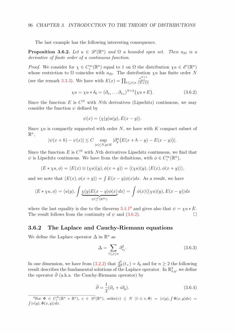
96 CHAPTER 3. INTRODUCTION TO THE THEORY OF DISTRIBUTIONS
The last example has the following interesting consequence.
Proposition 3.6.2. Let u ∈ D ′(Rn) and Ω a bounded open set. Then u|Ω is aderivative of finite order of a continuous function.
Proof. We consider for χ ∈ C∞c (Rn) equal to 1 on Ω the distribution χu ∈ E ′(Rn)whose restriction to Ω coincides with u|Ω. The distribution χu has finite order N
(see the remark 3.3.3). We have with E(x) =∏
1≤j≤nxN+1j,+
(N+1)!
χu = χu ∗ δ0 = (∂x1 . . . ∂xn)N+2(χu ∗ E
). (3.6.2)
Since the function E is CN with Nth derivatives (Lipschitz) continuous, we mayconsider the function ψ defined by
ψ(x) = 〈χ(y)u(y), E(x− y)〉.
Since χu is compactly supported with order N , we have with K compact subset ofRn,
|ψ(x+ h)− ψ(x)| ≤ C sup|α|≤N,y∈K
|∂αy(E(x+ h− y)− E(x− y)
)|.
Since the function E is CN with Nth derivatives Lipschitz continuous, we find thatψ is Lipschitz continuous. We have from the definitions, with φ ∈ C∞c (Rn),
〈E ∗ χu, φ〉 = 〈E(x)⊗ (χu)(y), φ(x+ y)〉 = 〈(χu)(y), 〈E(x), φ(x+ y)〉〉,
and we note that 〈E(x), φ(x+ y)〉 =∫E(x− y)φ(x)dx. As a result, we have
〈E ∗ χu, φ〉 = 〈u(y),
∫χ(y)E(x− y)φ(x)︸ ︷︷ ︸
∈CNc (R2n)
dx〉 =
∫φ(x)〈(χu)(y), E(x− y)〉dx
where the last equality is due to the theorem 3.4.16 and gives also that ψ = χu ∗E.The result follows from the continuity of ψ and (3.6.2).
3.6.2 The Laplace and Cauchy-Riemann equations
We define the Laplace operator ∆ in Rn as
∆ =∑
1≤j≤n
∂2xj. (3.6.3)
In one dimension, we have from (3.2.2) that d2
dt2(t+) = δ0 and for n ≥ 2 the following
result describes the fundamental solutions of the Laplace operator. In R2x,y, we define
the operator ∂ (a.k.a. the Cauchy-Riemann operator) by
∂ =1
2(∂x + i∂y). (3.6.4)
6For Φ ∈ CNc (Rn × Rn), v ∈ D ′(Rn), order(v) ≤ N 〈1 ⊗ v,Φ〉 = 〈v(y),∫
Φ(x, y)dx〉 =∫〈v(y),Φ(x, y)〉dx.
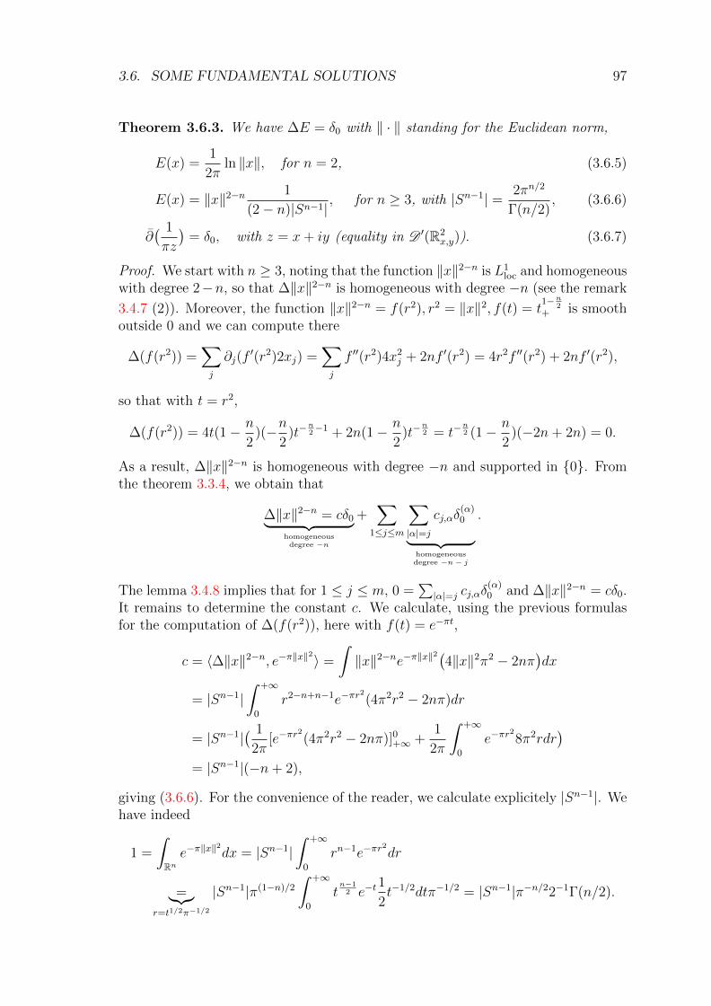
3.6. SOME FUNDAMENTAL SOLUTIONS 97
Theorem 3.6.3. We have ∆E = δ0 with ‖ · ‖ standing for the Euclidean norm,
E(x) =1
2πln ‖x‖, for n = 2, (3.6.5)
E(x) = ‖x‖2−n 1
(2− n)|Sn−1|, for n ≥ 3, with |Sn−1| = 2πn/2
Γ(n/2), (3.6.6)
∂( 1
πz
)= δ0, with z = x+ iy (equality in D ′(R2
x,y)). (3.6.7)
Proof. We start with n ≥ 3, noting that the function ‖x‖2−n is L1loc and homogeneous
with degree 2−n, so that ∆‖x‖2−n is homogeneous with degree −n (see the remark
3.4.7 (2)). Moreover, the function ‖x‖2−n = f(r2), r2 = ‖x‖2, f(t) = t1−n
2+ is smooth
outside 0 and we can compute there
∆(f(r2)) =∑j
∂j(f′(r2)2xj) =
∑j
f ′′(r2)4x2j + 2nf ′(r2) = 4r2f ′′(r2) + 2nf ′(r2),
so that with t = r2,
∆(f(r2)) = 4t(1− n
2)(−n
2)t−
n2−1 + 2n(1− n
2)t−
n2 = t−
n2 (1− n
2)(−2n+ 2n) = 0.
As a result, ∆‖x‖2−n is homogeneous with degree −n and supported in 0. Fromthe theorem 3.3.4, we obtain that
∆‖x‖2−n = cδ0︸ ︷︷ ︸homogeneousdegree −n
+∑
1≤j≤m
∑|α|=j
cj,αδ(α)0︸ ︷︷ ︸
homogeneousdegree −n− j
.
The lemma 3.4.8 implies that for 1 ≤ j ≤ m, 0 =∑|α|=j cj,αδ
(α)0 and ∆‖x‖2−n = cδ0.
It remains to determine the constant c. We calculate, using the previous formulasfor the computation of ∆(f(r2)), here with f(t) = e−πt,
c = 〈∆‖x‖2−n, e−π‖x‖2〉 =
∫‖x‖2−ne−π‖x‖
2(4‖x‖2π2 − 2nπ
)dx
= |Sn−1|∫ +∞
0
r2−n+n−1e−πr2
(4π2r2 − 2nπ)dr
= |Sn−1|( 1
2π[e−πr
2
(4π2r2 − 2nπ)]0+∞ +1
2π
∫ +∞
0
e−πr2
8π2rdr)
= |Sn−1|(−n+ 2),
giving (3.6.6). For the convenience of the reader, we calculate explicitely |Sn−1|. Wehave indeed
1 =
∫Rne−π‖x‖
2
dx = |Sn−1|∫ +∞
0
rn−1e−πr2
dr
=︸︷︷︸r=t1/2π−1/2
|Sn−1|π(1−n)/2
∫ +∞
0
tn−12 e−t
1
2t−1/2dtπ−1/2 = |Sn−1|π−n/22−1Γ(n/2).
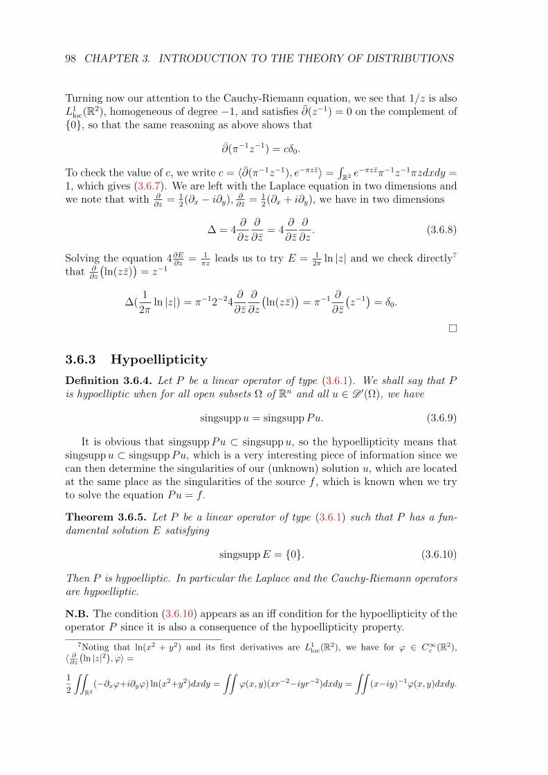
98 CHAPTER 3. INTRODUCTION TO THE THEORY OF DISTRIBUTIONS
Turning now our attention to the Cauchy-Riemann equation, we see that 1/z is alsoL1
loc(R2), homogeneous of degree −1, and satisfies ∂(z−1) = 0 on the complement of0, so that the same reasoning as above shows that
∂(π−1z−1) = cδ0.
To check the value of c, we write c = 〈∂(π−1z−1), e−πzz〉 =∫R2 e
−πzzπ−1z−1πzdxdy =1, which gives (3.6.7). We are left with the Laplace equation in two dimensions andwe note that with ∂
∂z= 1
2(∂x − i∂y), ∂∂z = 1
2(∂x + i∂y), we have in two dimensions
∆ = 4∂
∂z
∂
∂z= 4
∂
∂z
∂
∂z. (3.6.8)
Solving the equation 4∂E∂z
= 1πz
leads us to try E = 12π
ln |z| and we check directly7
that ∂∂z
(ln(zz)
)= z−1
∆(1
2πln |z|) = π−12−24
∂
∂z
∂
∂z
(ln(zz)
)= π−1 ∂
∂z
(z−1)
= δ0.
3.6.3 Hypoellipticity
Definition 3.6.4. Let P be a linear operator of type (3.6.1). We shall say that Pis hypoelliptic when for all open subsets Ω of Rn and all u ∈ D ′(Ω), we have
singsuppu = singsuppPu. (3.6.9)
It is obvious that singsuppPu ⊂ singsuppu, so the hypoellipticity means thatsingsuppu ⊂ singsuppPu, which is a very interesting piece of information since wecan then determine the singularities of our (unknown) solution u, which are locatedat the same place as the singularities of the source f , which is known when we tryto solve the equation Pu = f.
Theorem 3.6.5. Let P be a linear operator of type (3.6.1) such that P has a fun-damental solution E satisfying
singsuppE = 0. (3.6.10)
Then P is hypoelliptic. In particular the Laplace and the Cauchy-Riemann operatorsare hypoelliptic.
N.B. The condition (3.6.10) appears as an iff condition for the hypoellipticity of theoperator P since it is also a consequence of the hypoellipticity property.
7Noting that ln(x2 + y2) and its first derivatives are L1loc(R2), we have for ϕ ∈ C∞c (R2),
〈 ∂∂z(ln |z|2
), ϕ〉 =
1
2
∫∫R2
(−∂xϕ+i∂yϕ) ln(x2+y2)dxdy =
∫∫ϕ(x, y)(xr−2−iyr−2)dxdy =
∫∫(x−iy)−1ϕ(x, y)dxdy.
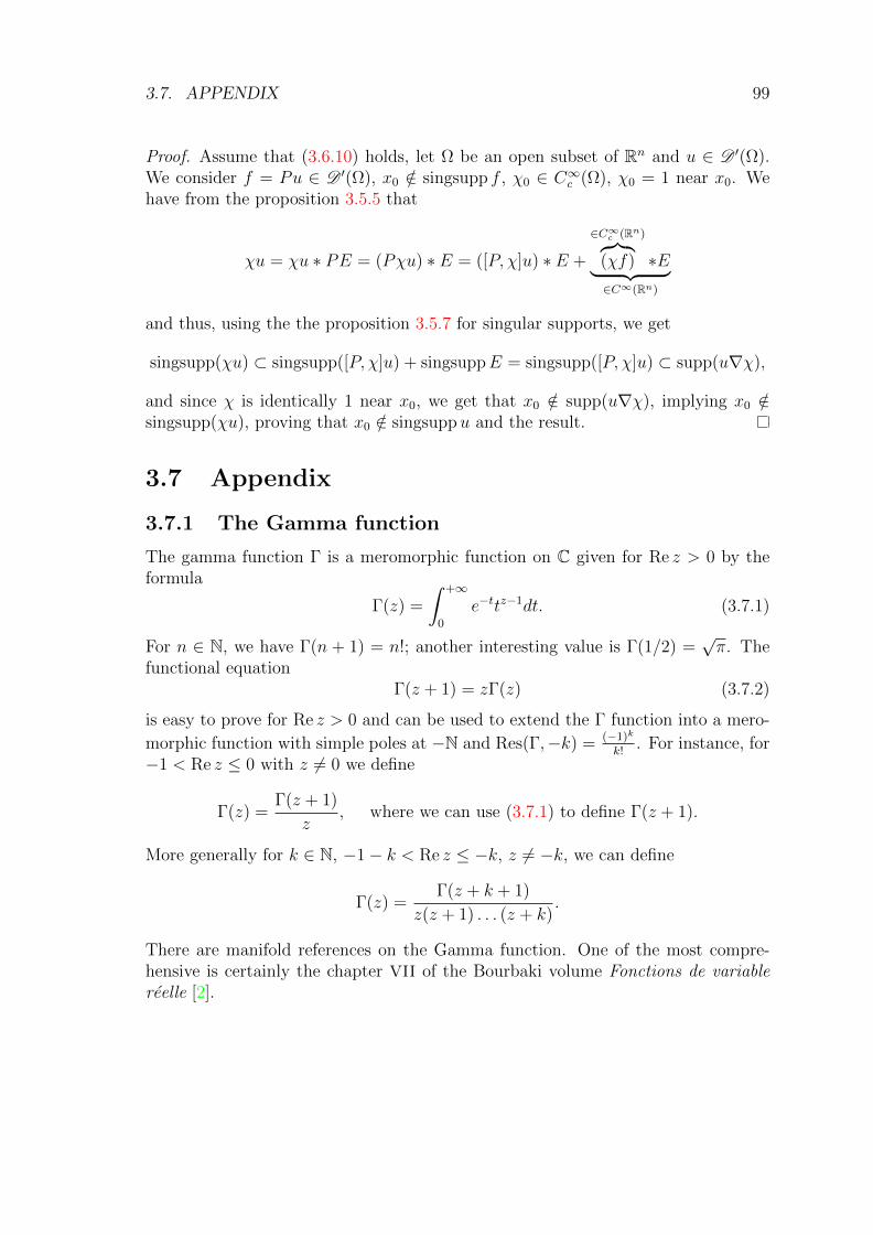
3.7. APPENDIX 99
Proof. Assume that (3.6.10) holds, let Ω be an open subset of Rn and u ∈ D ′(Ω).We consider f = Pu ∈ D ′(Ω), x0 /∈ singsupp f , χ0 ∈ C∞c (Ω), χ0 = 1 near x0. Wehave from the proposition 3.5.5 that
χu = χu ∗ PE = (Pχu) ∗ E = ([P, χ]u) ∗ E +
∈C∞c (Rn)︷︸︸︷(χf) ∗E︸ ︷︷ ︸∈C∞(Rn)
and thus, using the the proposition 3.5.7 for singular supports, we get
singsupp(χu) ⊂ singsupp([P, χ]u) + singsuppE = singsupp([P, χ]u) ⊂ supp(u∇χ),
and since χ is identically 1 near x0, we get that x0 /∈ supp(u∇χ), implying x0 /∈singsupp(χu), proving that x0 /∈ singsuppu and the result.
3.7 Appendix
3.7.1 The Gamma function
The gamma function Γ is a meromorphic function on C given for Re z > 0 by theformula
Γ(z) =
∫ +∞
0
e−ttz−1dt. (3.7.1)
For n ∈ N, we have Γ(n + 1) = n!; another interesting value is Γ(1/2) =√π. The
functional equationΓ(z + 1) = zΓ(z) (3.7.2)
is easy to prove for Re z > 0 and can be used to extend the Γ function into a mero-
morphic function with simple poles at −N and Res(Γ,−k) = (−1)k
k!. For instance, for
−1 < Re z ≤ 0 with z 6= 0 we define
Γ(z) =Γ(z + 1)
z, where we can use (3.7.1) to define Γ(z + 1).
More generally for k ∈ N, −1− k < Re z ≤ −k, z 6= −k, we can define
Γ(z) =Γ(z + k + 1)
z(z + 1) . . . (z + k).
There are manifold references on the Gamma function. One of the most compre-hensive is certainly the chapter VII of the Bourbaki volume Fonctions de variablereelle [2].

100 CHAPTER 3. INTRODUCTION TO THE THEORY OF DISTRIBUTIONS
Chapter 4
Introduction to Fourier Analysis
4.1 Fourier Transform of tempered distributions
4.1.1 The Fourier transformation on S (Rn)
Let n ≥ 1 be an integer. The Schwartz space S (Rn) is defined in the section 2.3.5,is a Frechet space, as the space of C∞ functions u from Rn to C such that, for allmulti-indices1 α, β ∈ Nn,
supx∈Rn|xα∂βxu(x)| < +∞.
A simple example of such a function is e−|x|2, (|x| is the Euclidean norm of x) and
more generally if A is a symmetric positive definite n× n matrix the function
vA(x) = e−π〈Ax,x〉
belongs to the Schwartz class.
Definition 4.1.1. For u ∈ S (Rn), we define its Fourier transform u as
u(ξ) =
∫Rne−2iπx·ξu(x)dx. (4.1.1)
Lemma 4.1.2. The Fourier transform sends continuously S (Rn) into itself.
Proof. Just notice that ξα∂βξ u(ξ) =∫e−2iπxξ∂αx (xβu)(x)dx(2iπ)|β|−|α|(−1)|β|.
Lemma 4.1.3. For a symmetric positive definite n× n matrix A, we have
vA(ξ) = (detA)−1/2e−π〈A−1ξ,ξ〉. (4.1.2)
1Here we use the multi-index notation: for α = (α1, . . . , αn) ∈ Nn we define
xα = xα11 . . . xαnn , ∂αx = ∂α1
x1. . . ∂αnxn , |α| =
∑1≤j≤n
αj .
101
102 CHAPTER 4. INTRODUCTION TO FOURIER ANALYSIS
Proof. In fact, diagonalizing the symmetric matrix A, it is enough to prove theone-dimensional version of (4.1.2), i.e. to check∫
e−2iπxξe−πx2
dx =
∫e−π(x+iξ)2dxe−πξ
2
= e−πξ2
,
where the second equality is obtained by taking the ξ-derivative of∫e−π(x+iξ)2dx :
we have indeed
d
dξ
(∫e−π(x+iξ)2dx
)=
∫e−π(x+iξ)2(−2iπ)(x+ iξ)dx = −i
∫d
dx
(e−π(x+iξ)2
)dx = 0.
For a > 0, we obtain∫R e−2iπxξe−πax
2dx = a−1/2e−πa
−1ξ2 , which is the sought resultin one dimension. If n ≥ 2, and A is a positive definite symmetric matrix, thereexists an orthogonal n× n matrix P (i.e. tPP = Id) such that
D =tPAP, D = diag(λ1, . . . , λn), all λj > 0.
As a consequence, we have, since | detP | = 1,∫Rne−2iπx·ξe−π〈Ax,x〉dx =
∫Rne−2iπ(Py)·ξe−π〈APy,Py〉dy =
∫Rne−2iπy·(tPξ)e−π〈Dy,y〉dy
(with η =tPξ) =∏
1≤j≤n
∫Re−2iπyjηje−πλjy
2j dyj =
∏1≤j≤n
λ−1/2j e−πλ
−1j η2j
= (detA)−1/2e−π〈D−1η,η〉 = (detA)−1/2e−π〈
tPA−1P tPξ,tPξ〉 = (detA)−1/2e−π〈A−1ξ,ξ〉.
Proposition 4.1.4. The Fourier transformation is an isomorphism of the Schwartzclass and for u ∈ S (Rn), we have
u(x) =
∫e2iπxξu(ξ)dξ. (4.1.3)
Proof. Using (4.1.2) we calculate for u ∈ S (Rn) and ε > 0, dealing with absolutelyconverging integrals,
uε(x) =
∫e2iπxξu(ξ)e−πε
2|ξ|2dξ
=
∫∫e2iπxξe−πε
2|ξ|2u(y)e−2iπyξdydξ
=
∫u(y)e−πε
−2|x−y|2ε−ndy
=
∫ (u(x+ εy)− u(x)
)︸ ︷︷ ︸with absolute value≤ε|y|‖u′‖L∞
e−π|y|2
dy + u(x).
Taking the limit when ε goes to zero, we get the Fourier inversion formula
u(x) =
∫e2iπxξu(ξ)dξ. (4.1.4)
4.1. FOURIER TRANSFORM OF TEMPERED DISTRIBUTIONS 103
We have also proven for u ∈ S (Rn) and u(x) = u(−x)
u =ˇu. (4.1.5)
Since u 7→ u and u 7→ u are continuous homomorphisms of S (Rn), this completesthe proof of the proposition.
Proposition 4.1.5. Using the notation
Dxj =1
2iπ
∂
∂xj, Dα
x =n∏j=1
Dαjxj
with α = (α1, . . . , αn) ∈ Nn, (4.1.6)
we have, for u ∈ S (Rn)
Dαxu(ξ) = ξαu(ξ), (Dα
ξ u)(ξ) = (−1)|α|xαu(x)(ξ) (4.1.7)
Proof. We have for u ∈ S (Rn), u(ξ) =∫e−2iπx·ξu(x)dx and thus
(Dαξ u)(ξ) = (−1)|α|
∫e−2iπx·ξxαu(x)dx,
ξαu(ξ) =
∫(−2iπ)−|α|∂αx
(e−2iπx·ξ)u(x)dx =
∫e−2iπx·ξ(2iπ)−|α|(∂αxu)(x)dx,
proving both formulas.
N.B. The normalization factor 12iπ
leads to a simplification in the formulas (4.1.7),but the most important aspect of these formulas is certainly that the Fourier trans-formation exchanges the operation of derivation against the operation of multiplica-tion. For instance if P (D) is given by a formula (3.6.1), we have
P u(ξ) =∑|α|≤m
aαξαu(ξ) = P (ξ)u(ξ).
Remark 4.1.6. We have the following continuous inclusions2
D(Rn) → S (Rn) → E (Rn), (4.1.8)
triggering the (continuous) inclusions of topological duals,
E ′(Rn) → S ′(Rn) → D ′(Rn). (4.1.9)
The space S ′(Rn) is the topological dual of the Frechet space S (Rn) and is calledthe space of tempered distributions on Rn. We shall sometimes omit the “Rn” inS (Rn),S ′(Rn), at least when it is clear that the dimension is fixed equal to n.
The Fourier transformation can be extended to S ′(Rn).
2The first inclusion is certainly sequentially continuous according to the definition 3.1.9 and thesecond is an inclusion of Frechet spaces: for each semi-norm p on E (Rn), there exists a semi-normq on S (Rn) such that for all u ∈ S (Rn), p(u) ≤ q(u).
104 CHAPTER 4. INTRODUCTION TO FOURIER ANALYSIS
4.1.2 The Fourier transformation on S ′(Rn)
Definition 4.1.7. Let T be a tempered distribution ; the Fourier transform T of Tis the tempered distibution defined by the formula
〈T , ϕ〉S ′,S = 〈T, ϕ〉S ′,S . (4.1.10)
The linear form T is obviously a tempered distribution since the Fourier transfor-mation is continuous on S . Thanks to the lemma 3.1.7, if T ∈ S , the presentdefinition of T and (4.1.1) coincide.
Note that for T, ϕ ∈ S , we have 〈T , ϕ〉 =∫∫
T (x)e−2iπx·ξϕ(ξ)dxdξ = 〈T, ϕ〉.This definition gives that
δ0 = 1, (4.1.11)
since 〈δ0, ϕ〉 = 〈δ0, ϕ〉 = ϕ(0) =∫ϕ(x)dx = 〈1, ϕ〉.
Theorem 4.1.8. The Fourier transformation is an isomorphism of S ′(Rn). Let Tbe a tempered distribution. Then we have3
T =ˇT. (4.1.12)
With obvious notations, we have the following extensions of (4.1.7),
DαxT (ξ) = ξαT (ξ), (Dα
ξ T )(ξ) = (−1)|α|xαT (x)(ξ). (4.1.13)
Proof. Using the notation (ϕ)(x) = ϕ(−x) for ϕ ∈ S , we define S for S ∈ S ′ by(see the remark 3.4.4), 〈S, ϕ〉S ′,S = 〈S, ϕ〉S ′,S and we obtain for T ∈ S ′
〈ˇT, ϕ〉S ′,S = 〈 ˆT , ϕ〉S ′,S = 〈T , ˆϕ〉S ′,S = 〈T, ˆϕ〉S ′,S = 〈T, ϕ〉S ′,S ,
where the last equality is due to the fact that ϕ 7→ ϕ commutes4 with the Fourier
transform and (4.1.4) meansˇϕ = ϕ, a formula also proven true on S ′ by the previous
line of equality. The formula (4.1.7) is true as well for T ∈ S ′ since, with ϕ ∈ Sand ϕα(ξ) = ξαϕ(ξ), we have
〈DαT , ϕ〉S ′,S = 〈T, (−1)|α|Dαϕ〉S ′,S = 〈T, ϕα〉S ′,S = 〈T , ϕα〉S ′,S ,
and the other part is proven the same way.
The following lemma will be useful.
Lemma 4.1.9. Let T ∈ S ′(Rn) be a homogeneous distribution of degree m. Thenits Fourier transform is a homogeneous distribution of degree −m− n
Proof. We check
(ξ ·Dξ)T = −ξ · xT = − (Dx · xT ) = − n
2iπT − 1
2iπ(x · ∂xT ) = −(n+m)
2iπT ,
so that the Euler equation (3.4.6) ξ∂ξT = −(n+m)T is satisfied.
3According to the remark 3.4.4, T is the distribution defined by 〈T , ϕ〉 = 〈T, ϕ〉 and if T ∈ S ′,T is also a tempered distribution since ϕ 7→ ϕ is an involutive isomorphism of S .
4If ϕ ∈ S , we have ϕ(ξ) =∫e−2iπx·ξϕ(−x)dx =
∫e2iπx·ξϕ(x)dx = ϕ(−ξ) = ˇϕ(ξ).
4.1. FOURIER TRANSFORM OF TEMPERED DISTRIBUTIONS 105
4.1.3 The Fourier transformation on L1(Rn)
Theorem 4.1.10. The Fourier transformation is linear continuous from L1(Rn)into L∞(Rn) and for u ∈ L1(Rn), we have
u(ξ) =
∫e−2iπx·ξu(x)dx, ‖u‖L∞(Rn) ≤ ‖u‖L1(Rn). (4.1.14)
Proof. The formula (4.1.1) can be used to define directly the Fourier transform ofa function in L1(Rn) and this gives an L∞(Rn) function which coincides with theFourier transform: for a test function ϕ ∈ S (Rn), and u ∈ L1(Rn), we have by thedefinition (4.1.10) above and the Fubini theorem
〈u, ϕ〉S ′,S =
∫u(x)ϕ(x)dx =
∫∫u(x)ϕ(ξ)e−2iπx·ξdxdξ =
∫u(ξ)ϕ(ξ)dξ
with u(ξ) =∫e−2iπx·ξu(x)dx which is thus the Fourier transform of u.
4.1.4 The Fourier transformation on L2(Rn)
We refer the reader to the section 5.3 in Chapter 5.
4.1.5 Some standard examples of Fourier transform
Let us consider the Heaviside function defined on R by H(x) = 1 for x > 0, H(x) = 0for x ≤ 0 ; it is obviously a tempered distribution, so that we can compute its Fouriertransform. With the notation of this section, we have, with δ0 the Dirac mass at 0,H(x) = H(−x),
H + H = 1 = δ0, H − H = sign,1
iπ=
1
2iπ2δ0(ξ) = D sign(ξ) = ξsignξ
so that ξ(signξ − 1
iπpv(1/ξ)
)= 0 and from the theorem 3.2.8, we get
signξ − 1
iπpv(1/ξ) = cδ0,
with c = 0 since the lhs is odd. We obtain
sign(ξ) =1
iπpv
1
ξ, (4.1.15)
pv(
1
πx) = −i sign ξ, (4.1.16)
H =δ0
2+
1
2iπpv(
1
ξ) =
1
(x− i0)
1
2iπ. (4.1.17)
Let us consider now for 0 < α < n the L1loc(Rn) function uα(x) = |x|α−n (|x| is
the Euclidean norm of x); since uα is also bounded for |x| ≥ 1, it is a tempereddistribution. Let us calculate its Fourier transform vα. Since uα is homogeneous ofdegree α − n, we get from the lemma 4.1.9 that vα is a homogeneous distribution
106 CHAPTER 4. INTRODUCTION TO FOURIER ANALYSIS
of degree −α. On the other hand, if S ∈ O(Rn) (the orthogonal group), we have inthe distribution sense (see the definition 3.4.3), since uα is a radial function,
vα(Sξ) = vα(ξ). (4.1.18)
The distribution |ξ|αvα(ξ) is homogeneous of degree 0 on Rn\0 and is also “radial”,i.e. satisfies (4.1.18). Moreover on Rn\0, the distribution vα is a C1 function whichcoincides with∫
e−2iπx·ξχ0(x)|x|α−ndx+ |ξ|−2N
∫e−2iπx·ξ|Dx|2N
(χ1(x)|x|α−n
)dx,
where χ0 ∈ C∞c (Rn) is 1 near 0 and χ1 = 1 − χ0, N ∈ N, α + 1 < 2N . As a result|ξ|αvα(ξ) = cα on Rn\0 and the distribution on Rn (note that α < n)
T = vα(ξ)− cα|ξ|−α
is supported in 0 and homogeneous (on Rn) with degree −α. From the theorem3.3.4 and the lemma 3.4.8, the condition 0 < α < n gives vα = cα|ξ|−α. To find cα,we compute ∫
|x|α−ne−πx2dx = 〈uα, e−πx2〉 = cα
∫|ξ|−αe−πξ2dξ
which yields
2−1Γ(α
2)π−
α2 =
∫ +∞
0
rα−1e−πr2
dr = cα
∫ +∞
0
rn−α−1e−πr2
dr
= cα2−1Γ(n− α
2)π−
n−α2 .
We have proven the following lemma.
Lemma 4.1.11. Let n ∈ N∗ and α ∈]0, n[. The function uα(x) = |x|α−n is L1loc(Rn)
and also a temperate distribution on Rn. Its Fourier transform vα is also L1loc(Rn)
and given by
vα(ξ) = |ξ|−απn2−α Γ(α
2)
Γ(n−α2
).
4.2 The Poisson summation formula
4.2.1 Wave packets
We define for x ∈ Rn, (y, η) ∈ Rn × Rn
ϕy,η(x) = 2n/4e−π(x−y)2e2iπ(x−y)·η = 2n/4e−π(x−y−iη)2e−πη2
, (4.2.1)
where for ζ = (ζ1, . . . , ζn) ∈ Cn, ζ2 =∑
1≤j≤n
ζ2j . (4.2.2)
We note that the function ϕy,η is in S(Rn) and with L2 norm 1. In fact, ϕy,η appearsas a phase translation of a normalized Gaussian. The following lemma introducesthe wave packets transform as a Gabor wavelet.
4.2. THE POISSON SUMMATION FORMULA 107
Lemma 4.2.1. Let u be a function in the Schwartz class S(Rn). We define
(Wu)(y, η) = (u, ϕy,η)L2(Rn) = 2n/4∫u(x)e−π(x−y)2e−2iπ(x−y)·ηdx (4.2.3)
= 2n/4∫u(x)e−π(y−iη−x)2dxe−πη
2
. (4.2.4)
For u ∈ L2(Rn), the function Tu defined by
(Tu)(y + iη) = eπη2
Wu(y,−η) = 2n/4∫u(x)e−π(y+iη−x)2dx (4.2.5)
is an entire function. The mapping u 7→ Wu is continuous from S(Rn) to S(R2n)and isometric from L2(Rn) to L2(R2n). Moreover, we have the reconstruction for-mula
u(x) =
∫∫Rn×Rn
Wu(y, η)ϕy,η(x)dydη. (4.2.6)
Proof. For u in S(Rn), we have
Wu(y, η) = e2iπyηΩ1
(η, y)
where Ω1
is the Fourier transform with respect to the first variable of the S(R2n)function Ω(x, y) = u(x)e−π(x−y)22n/4. Thus the function Wu belongs to S(R2n). Itmakes sense to compute
2−n/2(Wu,Wu)L2(R2n) =
limε→0+
∫u(x1)u(x2)e−π[(x1−y)2+(x2−y)2+2i(x1−x2)η+ε2η2]dydηdx1dx2. (4.2.7)
Now the last integral on R4n converges absolutely and we can use the Fubini theorem.Integrating with respect to η involves the Fourier transform of a Gaussian functionand we get ε−ne−πε
−2(x1−x2)2 . Since
2(x1 − y)2 + 2(x2 − y)2 = (x1 + x2 − 2y)2 + (x1 − x2)2,
integrating with respect to y yields a factor 2−n/2. We are left with
(Wu,Wu)L2(R2n) =
limε→0+
∫u(x1) u(x2)e−π(x1−x2)2/2ε−ne−πε
−2(x1−x2)2dx1dx2. (4.2.8)
Changing the variables, the integral is
limε→0+
∫u(s+ εt/2) u(s− εt/2)e−πε
2t2/2e−πt2
dtds = ‖u‖2L2(Rn)
by Lebesgue’s dominated convergence theorem: the triangle inequality and the es-timate |u(x)| ≤ C(1 + |x|)−n−1 imply, with v = u/C,
|v(s+ εt/2) v(s− εt/2)| ≤ (1 + |s+ εt/2|)−n−1(1 + |s+ εt/2|)−n−1
≤ (1 + |s+ εt/2|+ |s− εt/2|)−n−1
≤ (1 + 2|s|)−n−1.
108 CHAPTER 4. INTRODUCTION TO FOURIER ANALYSIS
Eventually, this proves that
‖Wu‖2L2(R2n) = ‖u‖2
L2(Rn) (4.2.9)
i.e.
W : L2(Rn)→ L2(R2n) with W ∗W = idL2(Rn). (4.2.10)
Noticing first that∫∫
Wu(y, η)ϕy,ηdydη belongs to L2(Rn) (with a norm smallerthan ‖Wu‖L1(R2n)) and applying Fubini’s theorem, we get from the polarization of(4.2.9) for u, v ∈ S(Rn),
(u, v)L2(Rn) = (Wu,Wv)L2(R2n)
=
∫∫Wu(y, η)(ϕy,η, v)L2(Rn)dydη
= (
∫∫Wu(y, η)ϕy,ηdydη, v)L2(Rn),
yielding the result of the lemma u =∫∫
Wu(y, η)ϕy,ηdydη.
4.2.2 Poisson’s formula
The following lemma is in fact the Poisson summation formula for Gaussian functionsin one dimension.
Lemma 4.2.2. For all complex numbers z, the following series are absolutely con-verging and ∑
m∈Z
e−π(z+m)2 =∑m∈Z
e−πm2
e2iπmz. (4.2.11)
Proof. We set ω(z) =∑
m∈Z e−π(z+m)2 . The function ω is entire and 1-periodic since
for all m ∈ Z, z 7→ e−π(z+m)2 is entire and for R > 0
sup|z|≤R
|e−π(z+m)2| ≤ sup|z|≤R
|e−πz2 |e−πm2
e2π|m|R ∈ l1(Z).
Consequently, for z ∈ R, we obtain, expanding ω in Fourier series5,
ω(z) =∑k∈Z
e2iπkz
∫ 1
0
ω(x)e−2iπkxdx.
5 Note that we use this expansion only for a C∞ 1-periodic function. The proof is simple and
requires only to compute 1 + 2 Re∑
1≤k≤N e2iπkx = sinπ(2N+1)x
sinπx . Then one has to show that for asmooth 1-periodic function ω such that ω(0) = 0,
limλ→+∞
∫ 1
0
sinλx
sinπxω(x)dx = 0,
which is obvious since for a smooth ν (here we take ν(x) = ω(x)/ sinπx), |∫ 1
0ν(x)sinλxdx| =
O(λ−1) by integration by parts.
4.3. FOURIER TRANSFORMATION AND CONVOLUTION 109
We also check, using Fubini’s theorem on L1(0, 1)× l1(Z)∫ 1
0
ω(x)e−2iπkxdx =∑m∈Z
∫ 1
0
e−π(x+m)2e−2iπkxdx
=∑m∈Z
∫ m+1
m
e−πt2
e−2iπktdt
=
∫Re−πt
2
e−2iπkt = e−πk2
.
So the lemma is proven for real z and since both sides are entire functions, weconclude by analytic continuation.
It is now straightforward to get the n-th dimensional version of the previouslemma: for all z ∈ Cn, using the notation (4.2.2), we have∑
m∈Zne−π(z+m)2 =
∑m∈Zn
e−πm2
e2iπm·z. (4.2.12)
Theorem 4.2.3 (The Poisson summation formula). Let n be a positive integer andu be a function in S(Rn). Then we have∑
k∈Znu(k) =
∑k∈Zn
u(k), (4.2.13)
where u stands for the Fourier transform of u. In other words the tempered distri-bution D0 =
∑k∈Zn δk is such that D0 = D0.
Proof. We write, according to (4.2.6) and to Fubini’s theorem∑k∈Zn u(k) =
∑k∈Zn
∫∫Wu(y, η)ϕy,η(k)dydη
=
∫∫Wu(y, η)
∑k∈Zn
ϕy,η(k)dydη.
Now, (4.2.12), (4.2.1) give∑
k∈Zn ϕy,η(k) =∑
k∈Zn ϕy,η(k), so that (4.2.6) and Fu-bini’s theorem imply the result.
4.3 Fourier transformation and convolution
4.3.1 Fourier transformation on E ′(Rn)
Theorem 4.3.1. Let u ∈ E ′(Rn). Then u is an entire function on Cn.
Proof. We have for ϕ ∈ D(Rn), according to the definition (3.4.14),
〈u, ϕ〉 = 〈u, ϕ〉 = 〈u(x),
∫e−2iπx·ξϕ(ξ)dξ〉 = 〈u(x)⊗ ϕ(ξ), e−2iπx·ξ〉E ′(R2n),E (R2n)
= 〈ϕ(ξ), 〈u(x), e−2iπx·ξ〉︸ ︷︷ ︸u(ξ)
〉,
110 CHAPTER 4. INTRODUCTION TO FOURIER ANALYSIS
an identity which implies u = u and moreover the function u is indeed entire, sincewith ζ ∈ Cn, and u(ζ) = 〈u(x), e−2iπx·ζ〉 the function u is C∞(Cn) from the corollary3.4.2, and we can check that ∂u = 0 (a direct computation of u(ζ+h)−u(ζ) provideselementarily the holomorphy of u).
Definition 4.3.2. The space OM(Rn) of multipliers of S (Rn) is the subspace of thefunctions f ∈ E (Rn) such that,
∀α ∈ Nn,∃Cα > 0,∃Nα ∈ N, ∀x ∈ Rn, |(∂αx f)(x)| ≤ Cα(1 + |x|)Nα . (4.3.1)
It is easy to check that, for f ∈ OM(Rn), the operator u 7→ fu is continuousfrom S (Rn) into itself, and by transposition from S ′(Rn) into itself: we have forT ∈ S ′(Rn), f ∈ OM(Rn),
〈fT, ϕ〉S ′,S = 〈T, fϕ〉S ′,S ,
and if p is a semi-norm of S , the continuity on S of the multiplication by f impliesthat there exists a semi-norm q on S such that for all ϕ ∈ S , p(fϕ) ≤ q(ϕ). Atypical example of a function in OM(Rn) is eiP (x) where P is a real-valued polynomial:in fact the derivatives of eiP (x) are of type Q(x)eiP (x) where Q is a polynomial sothat (4.3.1) holds.
Lemma 4.3.3. Let u ∈ E ′(Rn). Then u belongs to OM(Rn).
Proof. We have already seen that u(ξ) = 〈u(x), e−2iπx·ξ〉 is a smooth function so that
(Dαξ u)(ξ) = 〈u(x), e−2iπx·ξxα〉(−1)|α|
which implies |(Dαξ u)(ξ)| ≤ C0 sup |β|≤N0
x∈K0
|∂βx (e−2iπx·ξxα)| ≤ C1(1 + |ξ|)N0 , proving the
sought result.
4.3.2 Convolution and Fourier transformation
Theorem 4.3.4. Let u ∈ S ′(Rn), v ∈ E ′(Rn). Then the convolution u ∗ v belongsto S ′(Rn) and
u ∗ v = uv. (4.3.2)
N.B. We note that both sides of the equality (4.3.2) make sense since the lhs is theFourier transform of u ∗ v which belongs to S ′(this has to be proven) and v belongsto OM(Rn) so that the product of u ∈ S ′ with v makes sense.
Proof. Let us prove first that u ∗ v belongs to S ′. We have for ϕ ∈ D(Rn) andχ ∈ D(Rn) equal to 1 near the support of v,
〈u ∗ v, ϕ〉D ′(Rn),D(Rn) = 〈u(x)⊗ v(y), ϕ(x+ y)χ(y)〉D ′(R2n),D(R2n).
Now if ϕ ∈ S (Rn) the function (x, y) 7→ ϕ(x+y)χ(y) = Φ(x, y) belongs to S (R2n):it is a smooth function and xαyβ∂γx∂
ρyΦ is a linear combination of terms of type
(x+ y)ω(∂νϕ)(x+ y)yλ(∂µχ)(y)
4.4. SOME FUNDAMENTAL SOLUTIONS 111
which are bounded as product of bounded terms. Moreover, if Φ ∈ S (R2n), thefunction ψ(x) = 〈v(y),Φ(x, y)〉 is smooth (see the corollary 3.4.2(2)) and belongs toS (Rn) since xα(∂βxψ)(x) = 〈v(y), xα∂βxΦ(x, y)〉 and for some compact subset K0 ofRn,
|xα(∂βxψ)(x)| = |〈v(y), xα∂βxΦ(x, y)〉| ≤ C sup|γ|≤N0y∈K0
|xα∂βx∂γyΦ(x, y)| = p(Φ),
where p is a semi-norm on S (R2n). As a result, we can extend u ∗ v to a continuouslinear form on S (Rn) so that u ∗ v ∈ S ′(Rn). Let w ∈ S ′ such6 that w = uv. Forϕ ∈ S (Rn), we have
〈w,ϕ〉S ′,S = 〈uv, ˇϕ〉S ′,S = 〈u, v ˇϕ〉S ′,S .
On the other hand, we have
v(ξ) ˇϕ(ξ) = 〈v(x), e−2iπx·ξ〉∫ϕ(y)e2iπy·ξdy = 〈v(x)⊗ ϕ(y), e2iπ(y−x)·ξ〉
= 〈v(x), 〈ϕ(y), e2iπ(y−x)·ξ〉〉 = 〈v(x), 〈ϕ(y), e−2iπ(y+x)·ξ〉〉 = (v ∗ ϕ)(ξ),
so that
〈w,ϕ〉 = 〈u, (v ∗ ϕ)〉 = 〈u, v ∗ ϕ〉 = 〈u(−x), 〈v(x− y), ϕ(−y)〉〉= 〈u(x), 〈v(y − x), ϕ(y)〉〉 = 〈(u ∗ v), ϕ〉,
which gives w = u ∗ v and (4.3.2).
4.3.3 The Riemann-Lebesgue lemma
Lemma 4.3.5. Let u ∈ L1(Rn). Then from (4.1.14) u(ξ) =∫e−2iπx·ξu(x)dx; more-
over u belongs to C0(0)(Rn), where C0
(0)(Rn) stands for the space of continuous func-tions on Rn tending to 0 at infinity. In particular u is uniformly continuous.
Proof. This follows from the Riemann-Lebesgue lemma (see e.g. the lemma 3.4.4 in[9]); moreover,
|u(ξ + h)− u(ξ)| =∫|u(x)||e−2iπx·h − 1|dx = σu(h),
and the Lebesgue dominated convergence theorem implies that limh→0 σu(h) = 0,implying as well the uniform continuity.
4.4 Some fundamental solutions
4.4.1 The heat equation
The heat operator is the following constant coefficient differential operator on Rt×Rnx
∂t −∆x, (4.4.1)
where the Laplace operator ∆x on Rn is defined by (3.6.3).
6Take w =ˇuv .
112 CHAPTER 4. INTRODUCTION TO FOURIER ANALYSIS
Theorem 4.4.1. We define on Rt × Rnx the L1
loc function
E(t, x) = (4πt)−n/2H(t)e−|x|24t . (4.4.2)
The function E is C∞ on the complement of (0, 0) in R×Rn. The function E isa fundamental solution of the heat equation, i.e. ∂tE −∆xE = δ0(t)⊗ δ0(x).
Proof. To prove that E ∈ L1loc(Rn+1), we calculate for T ≥ 0,∫ T
0
∫ +∞
0
t−n/2rn−1e−r2
4t dtdr =︸︷︷︸r=2t1/2ρ
∫ T
0
∫ +∞
0
t−n/22n−1t(n−1)/2ρn−1e−ρ2
2t1/2dtdρ
= 2nT
∫ +∞
0
ρn−1e−ρ2
dρ < +∞.
Moreover, the function E is obviously analytic on the open subset of R1+n (t, x) ∈R × Rn, t 6= 0. Let us prove that E is C∞ on R × (Rn\0). With ρ0 defined in(3.1.1), the function ρ1 defined by ρ1(t) = H(t)t−n/2ρ0(t) is also C∞ on R and
E(t, x) = H(|x|2
4t)( |x|2
4t
)n/2e−|x|24t |x|−nπ−n/2 = |x|−nπ−n/2ρ1
( 4t
|x|2),
which is indeed smooth on Rt×(Rnx\0). We want to solve the equation ∂tu−∆xu =
δ0(t)δ0(x). If u belongs to S ′(Rn+1), we can consider its Fourier transform v withrespect to x (well-defined by transposition as the Fourier transform in (4.1.10)), andwe end-up with the simple ODE with parameters on v,
∂tv + 4π2|ξ|2v = δ0(t). (4.4.3)
It remains to determine a fundamental solution of that ODE: we have
d
dt+ λ = e−tλ
d
dtetλ,
( ddt
+ λ)(e−tλH(t)) =
(e−tλ
d
dtetλ)(e−tλH(t)) = δ0(t), (4.4.4)
so that we can take v = H(t)e−4π2t|ξ|2 , which belongs to S ′(Rt × Rnξ ). Taking
the inverse Fourier transform with respect to ξ of both sides of (4.4.3) gives7 withu ∈ S ′(Rt × Rn
ξ )∂tu−∆xu = δ0(t)⊗ δ0(x). (4.4.5)
To compute u, we check with ϕ ∈ D(R), ψ ∈ D(Rn),
〈u, ϕ⊗ ψ〉 = 〈vx, ϕ⊗ ψ〉 = 〈v, ϕ⊗ ψ〉 =
∫ +∞
0
∫Rnϕ(t)ψ(ξ)e−4π2t|ξ|2dtdξ.
We can use the Fubini theorem in that absolutely converging integral and use (4.1.2)to get
〈u, ϕ⊗ ψ〉 =
∫ +∞
0
ϕ(t)
(∫Rn
(4πt)−n/2e−π|x|24πt ψ(x)dx
)dt = 〈E,ϕ⊗ ψ〉,
where the last equality is due to the Fubini theorem and the local integrability ofE. We have thus E = u and E satisfies (4.4.5). The proof is complete.
7The Fourier transformation obviously respects the tensor products.
4.4. SOME FUNDAMENTAL SOLUTIONS 113
Corollary 4.4.2. The heat equation is C∞ hypoelliptic (see the definition 3.6.4) ,in particular for w ∈ D ′(R1+n),
singsuppw ⊂ singsupp(∂tw −∆xw),
where singsupp stands for the C∞ singular support as defined by (3.1.10).
Proof. It is an immediate consequence of the theorem 3.6.5, since E is C∞ outsidezero from the previous theorem.
Remark 4.4.3. It is also possible to define the analytic singular support of a dis-tribution T in an open subset Ω of Rn: we define
singsuppA T = x ∈ Ω,∀Uopen ∈ Vx, T|U /∈ A(U), (4.4.6)
whereA(U) stands for the analytic8 functions on the open set U . It is a consequence9
of the proof of theorem 4.4.1 that
singsuppAE = 0 × Rnx. (4.4.7)
In particular this implies that the heat equation is not analytic-hypoelliptic since
0 × Rnx = singsuppAE 6⊂ singsuppA(∂tE −∆xE) = singsuppA δ0 = 0R1+n.
4.4.2 The Schrodinger equation
We move forward now with the Schrodinger equation,
1
i
∂
∂t−∆x (4.4.8)
which looks similar to the heat equation, but which is in fact drastically different.
Lemma 4.4.4.
D(Rn+1) 7→∫ +∞
0
e−i(n−2)π4 (4πt)−n/2
(∫Rn
Φ(t, x)ei|x|24t dx
)dt = 〈E,Φ〉 (4.4.9)
is a distribution in Rn+1 of order ≤ n+ 2.
8A function f is said to be analytic on an open subset U of Rn if it is C∞(U), and for eachx0 ∈ U there exists r0 > 0 such that B(x0, r0) ⊂ U and
∀x ∈ B(x0, r0), f(x) =∑α∈Nn
1
α!∂αx f(x0)(x− x0)α.
9In fact, in the theorem, we have noted the obvious inclusion singsuppAE ⊂ 0 × Rnx , butsince E is C∞ in t 6= 0, vanishes identically on t < 0, is positive ( it means > 0) on t > 0, it cannotbe analytic near any point of 0 × Rnx .
114 CHAPTER 4. INTRODUCTION TO FOURIER ANALYSIS
Proof. Let Φ ∈ D(R× Rn); for t > 0 we have, using (4.6.7),
e−i(n−2)π4 (4πt)−n/2
∫Rn
Φ(t, x)ei|x|24t dx = i
∫Rn
Φx(t, ξ)e−4iπ2t|ξ|2dξ,
so that with N 3 n even > n, using (4.1.7) and (4.1.14),
supt>0
∣∣∣∣e−i(n−2)π4 (4πt)−n/2
∫Rn
Φ(t, x)ei|x|24t dx
∣∣∣∣ ≤ supt>0
∫Rn|Φx(t, ξ)|dξ
≤ supt>0
∫(1 + |ξ|2)−n/2| (1 + |ξ|2)n/2︸ ︷︷ ︸
polynomial
Φ(t, ξ)|dξ ≤ Cn max|α|≤n‖∂αxΦ‖L∞(Rn+1).
As a result the mapping
D(Rn+1) 7→∫ +∞
0
e−i(n−2)π4 (4πt)−n/2
(∫Rn
Φ(t, x)ei|x|24t dx
)dt = 〈E,Φ〉
is a distribution of order ≤ n+ 2.
Theorem 4.4.5. The distribution E given by (4.4.9) is a fundamental solution ofthe Schrodinger equation, i.e. 1
i∂tE −∆xE = δ0(t)⊗ δ0(x). Moreover, E is smooth
on the open set t 6= 0 and equal there to
e−i(n−2)π4H(t)(4πt)−n/2ei
|x|24t . (4.4.10)
The distribution E is the partial Fourier transform with respect to the variable x ofthe L∞(Rn+1) function
E(t, ξ) = iH(t)e−4iπ2t|ξ|2 . (4.4.11)
Proof. We want to solve the equation −i∂tu − ∆xu = δ0(t)δ0(x). If u belongs toS ′(Rn+1), we can consider its Fourier transform v with respect to x (well-defined bytransposition as the Fourier transform in (4.1.10)), and we end-up with the simpleODE with parameters on v,
∂tv + i4π2|ξ|2v = iδ0(t). (4.4.12)
Using the identity (4.4.4), we see that we can take v = iH(t)e−i4π2t|ξ|2 , which belongs
to S ′(Rt×Rnξ ). Taking the inverse Fourier transform with respect to ξ of both sides
of (4.4.12) gives with u ∈ S ′(Rt × Rnξ )
∂tu− i∆xu = iδ0(t)⊗ δ0(x) i.e.1
i∂tu−∆xu = δ0(t)⊗ δ0(x). (4.4.13)
To compute u, we check with ϕ ∈ D(R), ψ ∈ D(Rn),
〈u, ϕ⊗ ψ〉 = 〈vx, ϕ⊗ ψ〉 = 〈v, ϕ⊗ ˇψ〉 = i
∫ +∞
0
ϕ(t)
(∫Rnψ(ξ)eiπ(−4πt)|ξ|2dξ
)dt.
(4.4.14)
4.4. SOME FUNDAMENTAL SOLUTIONS 115
We note now that, using (4.6.7) and (4.1.10), for t > 0,
i
∫Rnψ(ξ)eiπ(−4πt)|ξ|2dξ = i
∫Rnψ(x)(4πt)−n/2ei
|x|24t dxe−n
iπ4
= e−i(n−2)π4 (4πt)−n/2
∫Rnei|x|24t ψ(x)dx.
As a result, u is a distribution on Rn+1 defined by
〈u,Φ〉 = e−i(n−2)π4 (4π)−n/2
∫ +∞
0
t−n/2(∫
RnΦ(t, x)ei
|x|24t dx
)dt
and coincides with E, so that E satisfies (4.4.13). The identity (4.4.14) is proving(4.4.11). The proof of the theorem is complete.
Remark 4.4.6. The fundamental solution of the Schrodinger equation is unboundednear t = 0 and, since E is smooth on t 6= 0, its C∞ singular support is equal to0 × Rn
x. In particular, the Schrodinger equation is not hypoelliptic. We shall seethat it looks like a propagation equation with an infinite speed, or more preciselywith a speed depending on the frequency of the wave.
4.4.3 The wave equation
Presentation
The wave equation in d dimensions with speed of propagation c > 0, is given by theoperator on Rt × Rd
x
c = c−2∂2t −∆x. (4.4.15)
We want to solve the equation c−2∂2t u−∆xu = δ0(t)δ0(x). If u belongs to S ′(Rd+1),
we can consider its Fourier transform v with respect to x, and we end-up with theODE with parameters on v,
c−2∂2t v + 4π2|ξ|2v = δ0(t), ∂2
t v + 4π2c2|ξ|2v = c2δ0(t). (4.4.16)
Lemma 4.4.7. Let λ, µ ∈ C. A fundamental solution of Pλ,µ = ( ddt−λ)( d
dt−µ) (on
the real line) is (etλ − etµλ− µ
)H(t) for λ 6= µ,
tetλH(t) for λ = µ.(4.4.17)
Proof. If λ 6= µ, to solve ( ddt− λ)( d
dt− µ) = δ0(t), the method of variation of
parameters gives a solution a(t)eλt + b(t)eµt with(etλ etµ
λetλ µetµ
)(a
b
)=
(0δ
)=⇒
(a
b
)=
1
λ− µ
(δ−δ
)=⇒ (4.4.17) for λ 6= µ,
which gives also the result for λ = µ by differentiation with respect to λ of theidentity Pλ,µ
(etλ − etµ
)= (λ− µ)δ.
116 CHAPTER 4. INTRODUCTION TO FOURIER ANALYSIS
Going back to the wave equation, we can take v as the temperate distribution10
given by
v(t, ξ) = c2H(t)e2iπct|ξ| − e−2iπct|ξ|
4iπc|ξ|= c2H(t)
sin(2πct|ξ|
)2πc|ξ|
. (4.4.18)
Taking the inverse Fourier transform with respect to ξ of both sides of (4.4.16) giveswith u ∈ S ′(Rt × Rd
ξ)
c−2∂2t u−∆xu = δ0(t)⊗ δ0(x). (4.4.19)
To compute u, we check with Φ ∈ D(R1+d),
〈u,Φ〉 = 〈vx(t, ξ),Φ(t,−ξ)〉 =
∫ +∞
0
∫Rn
Φx(t, ξ)csin(2πct|ξ|
)2π|ξ|
dξdt. (4.4.20)
We have found an expression for a fundamental solution of the wave equation in dspace dimensions and proven the following proposition.
Proposition 4.4.8. Let E+ be the temperate distribution on Rd+1 such that
E+
x(t, ξ) = cH(t)
sin(2πct|ξ|
)2π|ξ|
. (4.4.21)
Then E+ is a fundamental solution of the wave equation (4.4.15), i.e. satisfiescE+ = δ0(t)⊗ δ0(x).
Remark 4.4.9. Defining the forward-light-cone Γ+,c as
Γ+,c = (t, x) ∈ R× Rd, ct ≥ |x|, (4.4.22)
one can prove more precisely that E+ is the only fundamental solution with supportin t ≥ 0 and that
suppE+ = Γ+, when d = 1 and d ≥ 2 is even, (4.4.23)
suppE+ = ∂Γ+, when d ≥ 3 is odd, (4.4.24)
singsuppE+ = ∂Γ+, in any dimension. (4.4.25)
Lemma 4.4.10. Let E1, E2 be fundamental solutions of the wave equation such thatsuppE1 ⊂ Γ+,c, suppE2 ⊂ t ≥ 0. Then E1 = E2.
Proof. Defining u = E1 − E2, we have suppu ⊂ t ≥ 0 and the mapping
t ≥ 0 × Γ+,c 3((t, x), (s, y)
)7→ (t+ s, x+ y) ∈ Rd+1
is proper since
t, s ≥ 0, cs ≥ |y|, |t+ s| ≤ T, |x+ y| ≤ R =⇒ t, s ∈ [0, T ], |x| ≤ R + cT, |y| ≤ cT,
so that the section 3.5.3 allows to perform the following calculations
u = u ∗ δ0 = u ∗cE1 = cu ∗ E1 = 0.
10The function R 3 s 7→ sin ss =
∑k≥0(−1)k s2k
(2k+1)! = S(s2) is a smooth bounded function of
s2, so that v(t, ξ) = c2H(t)tS(4π2c2t2|ξ|2) is continuous and such that |v(t, ξ)| ≤ CtH(t), thus atempered distribution.
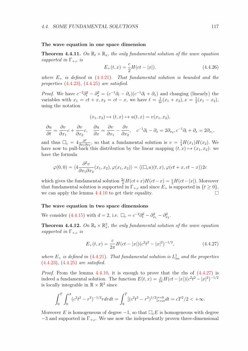
4.4. SOME FUNDAMENTAL SOLUTIONS 117
The wave equation in one space dimension
Theorem 4.4.11. On Rt×Rx, the only fundamental solution of the wave equationsupported in Γ+,c is
E+(t, x) =c
2H(ct− |x|). (4.4.26)
where E+ is defined in (4.4.21). That fundamental solution is bounded and theproperties (4.4.23), (4.4.25) are satisfied.
Proof. We have c−2∂2t − ∂2
x = (c−1∂t − ∂x)(c−1∂t + ∂x) and changing (linearly) thevariables with x1 = ct + x, x2 = ct − x, we have t = 1
2c(x1 + x2), x = 1
2(x1 − x2),
using the notation
(x1, x2) 7→ (t, x) 7→ u(t, x) = v(x1, x2),
∂u
∂t=
∂v
∂x1
c+∂v
∂x2
c,∂u
∂x=
∂v
∂x1
− ∂v
∂x2
, c−1∂t − ∂x = 2∂x2 , c−1∂t + ∂x = 2∂x1 ,
and thus c = 4 ∂2
∂x1∂x2, so that a fundamental solution is v = 1
4H(x1)H(x2). We
have now to pull-back this distribution by the linear mapping (t, x) 7→ (x1, x2): wehave the formula
ϕ(0, 0) = 〈4 ∂2v
∂x1∂x2
(x1, x2), ϕ(x1, x2)〉 = 〈(cu)(t, x), ϕ(ct+ x, ct− x)〉2c
which gives the fundamental solution 2c4H(ct+x)H(ct−x) = c
2H(ct−|x|). Moreover
that fundamental solution is supported in Γ+,c and since E+ is supported in t ≥ 0,we can apply the lemma 4.4.10 to get their equality.
The wave equation in two space dimensions
We consider (4.4.15) with d = 2, i.e. c = c−2∂2t − ∂2
x1− ∂2
x2.
Theorem 4.4.12. On Rt×R2x, the only fundamental solution of the wave equation
supported in Γ+,c is
E+(t, x) =c
2πH(ct− |x|)(c2t2 − |x|2)−1/2, (4.4.27)
where E+ is defined in (4.4.21). That fundamental solution is L1loc and the properties
(4.4.23), (4.4.25) are satisfied.
Proof. From the lemma 4.4.10, it is enough to prove that the rhs of (4.4.27) isindeed a fundamental solution. The function E(t, x) = c
2πH(ct−|x|)(c2t2−|x|2)−1/2
is locally integrable in R× R2 since∫ T
0
∫ ct
0
(c2t2 − r2)−1/2rdrdt =
∫ T
0
[(c2t2 − r2)1/2]r=0r=ctdt = cT 2/2 < +∞.
Moreover E is homogeneous of degree −1, so that cE is homogeneous with degree−3 and supported in Γ+,c. We use now the independently proven three-dimensional
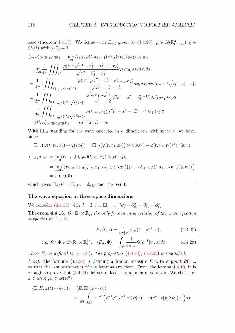
118 CHAPTER 4. INTRODUCTION TO FOURIER ANALYSIS
case (theorem 4.4.13). We define with E+,3 given by (4.4.29), ϕ ∈ D(R3t,x1,x2
), χ ∈D(R) with χ(0) = 1,
〈u, ϕ〉D ′(R3),D(R3) = limε→0〈E+,3, ϕ(t, x1, x2)⊗ χ(εx3)〉D ′(R4),D(R4)
= limε→0
1
4π
∫∫∫R3
ϕ(c−1√x2
1 + x22 + x2
3, x1, x2)√x2
1 + x22 + x2
3
χ(εx3)dx1dx2dx3
=1
4π2
∫∫∫R2x1,x2
×x3≥0
ϕ(c−1√x2
1 + x22 + x2
3, x1, x2)√x2
1 + x22 + x2
3
dx1dx2dx3(t = c−1√x2
1 + x22 + x2
3)
=1
2π
∫∫∫R2x1,x2
×ct≥√x21+x22
ϕ(t, x1, x2)
ct
1
2(c2t2 − x2
1 − x22)−1/22c2tdx1dx2dt
=c
2π
∫∫∫R2x1,x2
×ct≥√x21+x22
ϕ(t, x1, x2)(c2t2 − x21 − x2
2)−1/2dx1dx2dt
= 〈E,ϕ〉D ′(R3),D(R3), so that E = u.
With c,d standing for the wave operator in d dimensions with speed c, we have,since
c,3(ϕ(t, x1, x2)⊗ χ(εx3)
)= c,2
(ϕ(t, x1, x2)
)⊗ χ(εx3)− ϕ(t, x1, x2)ε2χ′′(εx3)
〈c,2u, ϕ〉 = limε→0〈E+,3, (c,2ϕ)(t, x1, x2)⊗ χ(εx3)〉
= limε→0
(〈E+,3,c,3
(ϕ(t, x1, x2)⊗ χ(εx3)
))〉+ 〈E+,3, ϕ(t, x1, x2)ε2χ′′(εx3)〉
)= ϕ(0, 0, 0),
which gives c,2E = c,2u = δ0,R3 and the result.
The wave equation in three space dimensions
We consider (4.4.15) with d = 3, i.e. c = c−2∂2t − ∂2
x1− ∂2
x2− ∂2
x3.
Theorem 4.4.13. On Rt×R3x, the only fundamental solution of the wave equation
supported in Γ+,c is
E+(t, x) =1
4π|x|δ0,R(t− c−1|x|), (4.4.28)
i.e. for Φ ∈ D(Rt × R3x), 〈E+,Φ〉 =
∫R3
1
4π|x|Φ(c−1|x|, x)dx. (4.4.29)
where E+ is defined in (4.4.21). The properties (4.4.24), (4.4.25) are satisfied.
Proof. The formula (4.4.29) is defining a Radon measure E with support ∂Γ+,c,so that the last statements of the lemmas are clear. From the lemma 4.4.10, it isenough to prove that (4.4.29) defines indeed a fundamental solution. We check forϕ ∈ D(R), ψ ∈ D(R3)
〈cE,ϕ(t)⊗ ψ(x)〉 = 〈E,c(ϕ⊗ ψ)〉
=1
4π
∫R3
|x|−1(c−2ϕ′′(c−1|x|)ψ(x)− ϕ(c−1|x|)(∆ψ)(x)
)dx.
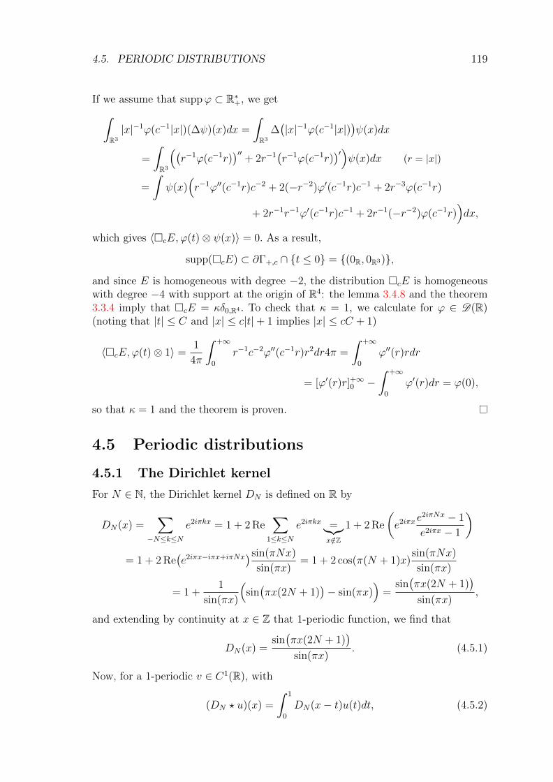
4.5. PERIODIC DISTRIBUTIONS 119
If we assume that suppϕ ⊂ R∗+, we get∫R3
|x|−1ϕ(c−1|x|)(∆ψ)(x)dx =
∫R3
∆(|x|−1ϕ(c−1|x|)
)ψ(x)dx
=
∫R3
((r−1ϕ(c−1r)
)′′+ 2r−1
(r−1ϕ(c−1r)
)′)ψ(x)dx (r = |x|)
=
∫ψ(x)
(r−1ϕ′′(c−1r)c−2 + 2(−r−2)ϕ′(c−1r)c−1 + 2r−3ϕ(c−1r)
+ 2r−1r−1ϕ′(c−1r)c−1 + 2r−1(−r−2)ϕ(c−1r))dx,
which gives 〈cE,ϕ(t)⊗ ψ(x)〉 = 0. As a result,
supp(cE) ⊂ ∂Γ+,c ∩ t ≤ 0 = (0R, 0R3),
and since E is homogeneous with degree −2, the distribution cE is homogeneouswith degree −4 with support at the origin of R4: the lemma 3.4.8 and the theorem3.3.4 imply that cE = κδ0,R4 . To check that κ = 1, we calculate for ϕ ∈ D(R)(noting that |t| ≤ C and |x| ≤ c|t|+ 1 implies |x| ≤ cC + 1)
〈cE,ϕ(t)⊗ 1〉 =1
4π
∫ +∞
0
r−1c−2ϕ′′(c−1r)r2dr4π =
∫ +∞
0
ϕ′′(r)rdr
= [ϕ′(r)r]+∞0 −∫ +∞
0
ϕ′(r)dr = ϕ(0),
so that κ = 1 and the theorem is proven.
4.5 Periodic distributions
4.5.1 The Dirichlet kernel
For N ∈ N, the Dirichlet kernel DN is defined on R by
DN(x) =∑
−N≤k≤N
e2iπkx = 1 + 2 Re∑
1≤k≤N
e2iπkx =︸︷︷︸x/∈Z
1 + 2 Re
(e2iπx e
2iπNx − 1
e2iπx − 1
)= 1 + 2 Re
(e2iπx−iπx+iπNx
)sin(πNx)
sin(πx)= 1 + 2 cos(π(N + 1)x)
sin(πNx)
sin(πx)
= 1 +1
sin(πx)
(sin(πx(2N + 1)
)− sin(πx)
)=
sin(πx(2N + 1)
)sin(πx)
,
and extending by continuity at x ∈ Z that 1-periodic function, we find that
DN(x) =sin(πx(2N + 1)
)sin(πx)
. (4.5.1)
Now, for a 1-periodic v ∈ C1(R), with
(DN ? u)(x) =
∫ 1
0
DN(x− t)u(t)dt, (4.5.2)
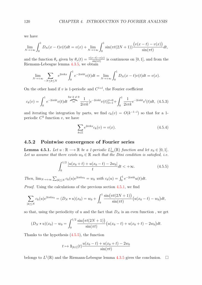
120 CHAPTER 4. INTRODUCTION TO FOURIER ANALYSIS
we have
limN→+∞
∫ 1
0
DN(x− t)v(t)dt = v(x) + limN→+∞
∫ 1
0
sin(πt(2N + 1))
(v(x− t)− v(x)
)sin(πt)
dt,
and the function θx given by θx(t) = v(x−t)−v(x)sin(πt)
is continuous on [0, 1], and from theRiemann-Lebesgue lemma 4.3.5, we obtain
limN→+∞
∑−N≤k≤N
e2iπkx
∫ 1
0
e−2iπktv(t)dt = limN→+∞
∫ 1
0
DN(x− t)v(t)dt = v(x).
On the other hand if v is 1-periodic and C1+l, the Fourier coefficient
ck(v) =
∫ 1
0
e−2iπktv(t)dtfor k 6= 0︷︸︸︷
=1
2iπk[e−2iπktv(t)]t=0
t=1+
∫ 1
0
1
2iπke−2iπktv′(t)dt, (4.5.3)
and iterating the integration by parts, we find ck(v) = O(k−1−l) so that for a 1-periodic C2 function v, we have∑
k∈Z
e2iπkxck(v) = v(x). (4.5.4)
4.5.2 Pointwise convergence of Fourier series
Lemma 4.5.1. Let u : R −→ R be a 1-periodic L1loc(R) function and let x0 ∈ [0, 1].
Let us assume that there exists w0 ∈ R such that the Dini condition is satisfied, i.e.∫ 1/2
0
|u(x0 + t) + u(x0 − t)− 2w0|t
dt < +∞. (4.5.5)
Then, limN→+∞∑|k|≤N ck(u)e2iπkx0 = w0 with ck(u) =
∫ 1
0e−2iπtku(t)dt.
Proof. Using the calculations of the previous section 4.5.1, we find
∑|k|≤N
ck(u)e2iπkx0 = (DN ∗ u)(x0) = w0 +
∫ 1
0
sin(πt(2N + 1)
)sin(πt)
(u(x0 − t)− w0
)dt,
so that, using the periodicity of u and the fact that DN is an even function , we get
(DN ∗ u)(x0)− w0 =
∫ 1/2
0
sin(πt(2N + 1)
)sin(πt)
(u(x0 − t) + u(x0 + t)− 2w0
)dt.
Thanks to the hypothesis (4.5.5), the function
t 7→ 1[0,1](t)u(x0 − t) + u(x0 + t)− 2w0
sin(πt)
belongs to L1(R) and the Riemann-Lebesgue lemma 4.3.5 gives the conclusion.
4.5. PERIODIC DISTRIBUTIONS 121
Theorem 4.5.2. Let u : R −→ R be a 1-periodic L1loc function.
(1) Let x0 ∈ [0, 1], w0 ∈ R. We define ωx0,w0(t) = |u(x0 + t) + u(x0 − t)− 2w0| andwe assume that ∫ 1/2
0
ωx0,w0(t)dt
t< +∞. (4.5.6)
Then the Fourier series (DN ∗ u)(x0) converges with limit w0. In particular, if(4.5.6) is satisfied with w0 = u(x0), the Fourier series (DN ∗ u)(x0) converges withlimit u(x0). If u has a left and right limit at x0 and is such that (4.5.6) is satisfiedwith w0 = 1
2
(u(x0 + 0) + u(x0 − 0)
), the Fourier series (DN ∗ u)(x0) converges with
limit 12
(u(x0 − 0) + u(x0 + 0)
).
(2) If the function u is Holder-continuous11, the Fourier series (DN ∗u)(x) convergesfor all x ∈ R with limit u(x).(3) If u has a left and right limit at each point and a left and right derivative at eachpoint, the Fourier series (DN ∗u)(x) converges for all x ∈ R with limit 1
2
(u(x− 0) +
u(x+ 0)).
Proof. (1) follows from the lemma 4.5.1; to obtain (2), we note that for a Holdercontinuous function of index θ ∈]0, 1], we have for t ∈]0, 1/2]
t−1ωx,u(x)(t) ≤ Ctθ−1 ∈ L1([0, 1/2]).
If u has a right-derivative at x0, it means that
u(x0 + t) = u(x0 + 0) + u′r(x0)t+ tε0(t), limt→0+
ε0(t) = 0.
As a consequence, for t ∈]0, 1/2], t−1|u(x0 + t)− u(x0 + 0)| ≤ |u′r(x0) + ε0(t)|. Sincelimt→0+ ε0(t) = 0, there exists T0 ∈]0, 1/2] such that |ε0(t)| ≤ 1 for t ∈ [0, T0]. As aresult, we have∫ 1/2
0
t−1|u(x0 + t)− u(x0 + 0)|dt
≤∫ T0
0
(|u′r(x0)|+ 1)dt+
∫ 1/2
T0
|u(x0 + t)− u(x0 + 0)|dtT−10 < +∞,
since u is also L1loc. The integral
∫ 1/2
0t−1|u(x0 − t) − u(x0 − 0)|dt is also finite and
the condition (4.5.6) holds with w0 = 12
(u(x0 − 0) + u(x0 + 0)
). The proof of the
lemma is complete.
4.5.3 Periodic distributions
We consider now a distribution u on Rn which is periodic with periods Zn. Letχ ∈ C∞c (Rn) such that χ = 1 on [0, 1]n. Then the function χ1 defined by
χ1(x) =∑k∈Zn
χ(x− k)
11 Holder-continuity of index θ ∈]0, 1] means that ∃C > 0,∀t, s, |u(t)− u(s)| ≤ C|t− s|θ.
122 CHAPTER 4. INTRODUCTION TO FOURIER ANALYSIS
is C∞ periodic12 with periods Zn. Moreover since Rn 3 x ∈∏
1≤j≤n[E(xj), E(xj)+1[,the bounded function χ1 is also bounded from below and such that 1 ≤ χ1(x). Withχ0 = χ/χ1, we have ∑
k∈Znχ0(x− k) = 1, χ0 ∈ C∞c (Rn).
For ϕ ∈ C∞c (Rn), we have from the periodicity of u
〈u, ϕ〉 =∑k∈Zn〈u(x), ϕ(x)χ0(x− k)〉 =
∑k∈Zn〈u(x), ϕ(x+ k)χ0(x)〉,
where the sums are finite. Now if ϕ ∈ S (Rn), we have, since χ0 is compactlysupported in |x| ≤ R0,
|〈u(x), ϕ(x+ k)χ0(x)〉| ≤ C0 sup|α|≤N0,|x|≤R0
|ϕ(α)(x+ k)|
≤ C0 sup|α|≤N0,|x|≤R0
|(1 +R0 + |x+ k|)n+1ϕ(α)(x+ k)|(1 + |k|)−n−1
≤ p0(ϕ)(1 + |k|)−n−1,
where p0 is a semi-norm of ϕ (independent of k). As a result u is a tempereddistribution and we have for ϕ ∈ S (Rn),
〈u, ϕ〉 = 〈u(x),∑k∈Zn
ϕ(x+ k)χ0(x)︸ ︷︷ ︸ψx(k)
〉 = 〈u(x),∑k∈Zn
ψx(k)〉.
Now we see that ψx(k) =∫Rn ϕ(x + t)χ0(x)e−2iπktdt = χ0(x)e2iπkxϕ(k), so that
〈u, ϕ〉 =∑
k∈Zn〈u(x), χ0(x)e2iπkx〉ϕ(k) which means
u(x) =∑k∈Zn〈u(t), χ0(t)e2iπkt〉e−2iπkx =
∑k∈Zn〈u(t), χ0(t)e−2iπkt〉e2iπkx.
Theorem 4.5.3. Let u be a periodic distribution on Rn with periods Zn. Then u is atempered distribution and if χ0 is a C∞c (Rn) function such that
∑k∈Zn χ0(x−k) = 1,
we have
u =∑k∈Zn
ck(u)e2iπkx, (4.5.7)
u =∑k∈Zn
ck(u)δk, with ck(u) = 〈u(t), χ0(t)e−2iπkt〉, (4.5.8)
and convergence in S ′(Rn). If u is in Cm(Rn) with m > n, the previous formulashold with uniform convergence for (4.5.7) and
ck(u) =
∫[0,1]n
u(t)e−2iπktdt. (4.5.9)
12Note that the sum is locally finite since for K compact subset of Rn, (K − k) ∩ suppχ0 = ∅except for a finite subset of k ∈ Zn.
4.5. PERIODIC DISTRIBUTIONS 123
Proof. The first statements are already proven and the calculation of u is immediate.If u belongs to L1
loc we can redo the calculations above choosing χ0 = 1[0,1]n and get(4.5.7) with ck given by (4.5.9). Moreover, if u is in Cm with m > n, we get byintegration by parts that ck(u) is O(|k|−m) so that the series (4.5.7) is uniformlyconverging.
Theorem 4.5.4. Let u be a periodic distribution on Rn with periods Zn. If u ∈ L2loc
(i.e. u ∈ L2(Tn) with Tn = (R/Z)n), then
u(x) =∑k∈Zn
ck(u)e2iπkx, with ck(u) =
∫[0,1]n
u(t)e−2iπktdt, (4.5.10)
and convergence in L2(Tn). Moreover ‖u‖2L2(Tn) =
∑k∈Zn |ck(u)|2. Conversely, if the
coefficients ck(u) defined by (4.5.8) are in `2(Zn), the distribution u is L2(Tn)
Proof. As said above the formula for the ck(u) follows from changing the choice ofχ0 to 1[0,1]n in the discussion preceding the theorem 4.5.3. The formula (4.5.7) givesthe convergence in S ′(Rn) to u. Now, since
∫[0,1]n
e2iπ(k−l)tdt = δk,l we see from the
theorem 4.5.3 that for u ∈ Cn+1(Tn), 〈u, u〉L2(Tn) =∑
k∈Zn |ck(u)|2. As a consequencethe mapping L2(Tn) 3 u 7→ (ck(u))k∈Zn ∈ `2(Zn) is isometric with a range containingthe dense subset `1(Zn) (if (ck(u))k∈Zn ∈ `1(Zn), u is a continuous function); sincethe range is closed, the mapping is onto and is an isometric isomorphism from theopen mapping theorem.
124 CHAPTER 4. INTRODUCTION TO FOURIER ANALYSIS
4.6 Appendix
4.6.1 The logarithm of a nonsingular symmetric matrix
The set C\R− is star-shaped with respect to 1, so that we can define the principaldetermination of the logarithm for z ∈ C\R− by the formula
Log z =
∮[1,z]
dζ
ζ. (4.6.1)
The function Log is holomorphic on C\R− and we have Log z = ln z for z ∈ R∗+and by analytic continuation eLog z = z for z ∈ C\R−. We get also by analyticcontinuation, that Log ez = z for | Im z| < π.
Let Υ+ be the set of symmetric nonsingular n×n matrices with complex entriesand nonnegative real part. The set Υ+ is star-shaped with respect to the Id: forA ∈ Υ+, the segment [1, A] =
((1−t) Id +tA
)t∈[0,1]
is obviously made with symmetric
matrices with nonnegative real part which are invertible13, since for 0 ≤ t < 1,Re((1− t) Id +tA
)≥ (1 − t) Id > 0 and for t = 1, A is assumed to be invertible.
We can now define for A ∈ Υ+
LogA =
∫ 1
0
(A− I)(I + t(A− I)
)−1dt. (4.6.2)
We note that A commutes with (I + sA) (and thus with LogA), so that, for θ > 0,
d
dθLog(A+ θI) =
∫ 1
0
(I + t(A+ θI − I)
)−1dt
−∫ 1
0
(A+ θI − I
)t(I + t(A+ θI − I)
)−2dt,
and since ddt
(I+ t(A+θI−I)
)−1
= −(I+ t(A+θI−I)
)−2(A+θI−I), we obtain
by integration by parts ddθ
Log(A + θI) = (A + θI)−1. As a result, we find that forθ > 0, A ∈ Υ+, since all the matrices involved are commuting,
d
dθ
((A+ θI)−1eLog(A+θI)
)= 0,
so that, using the limit θ → +∞, we get that ∀A ∈ Υ+,∀θ > 0, eLog(A+θI) = (A+θI),and by continuity
∀A ∈ Υ+, eLogA = A, which implies detA = etrace LogA. (4.6.3)
Using (4.6.3), we can define for A ∈ Υ+, using (4.6.2)
(detA)−1/2 = e−12
trace LogA = | detA|−1/2e−i2
Im(trace LogA). (4.6.4)
13Note that a symmetric matrix B with a positive-definite real part is indeed invertible since foru ∈ Cn, Bu = 0 implies 0 = Re〈Bu, u〉 = 〈(ReB)u, u〉 ≥ c0‖u‖2 with c0 > 0 and thus u = 0.
4.6. APPENDIX 125
• When A is a positive definite matrix, LogA is real-valued and (detA)−1/2 =| detA|−1/2.
• When A = −iB where B is a real nonsingular symmetric matrix, we note thatB = PDtP with P ∈ O(n) and D diagonal. We see directly on the formulas(4.6.2),(4.6.1) that
LogA = Log(−iB) = P (Log(−iD))tP, trace LogA = trace Log(−iD)
and thus, with (µj) the (real) eigenvalues of B, we have Im (trace LogA) =Im∑
1≤j≤n Log(−iµj), where the last Log is given by (4.6.1). Finally we get,
Im (trace LogA) = −π2
∑1≤j≤n
signµj = −π2
signB
where signB is the signature of B. As a result, we have when A = −iB, Breal symmetric nonsingular matrix
(detA)−1/2 = | detA|−1/2eiπ4
sign(iA) = | detB|−1/2eiπ4
signB. (4.6.5)
4.6.2 Fourier transform of Gaussian functions
Proposition 4.6.1. Let A be a symmetric nonsingular n × n matrix with complexentries such that ReA ≥ 0. We define the Gaussian function vA on Rn by vA(x) =e−π〈Ax,x〉. The Fourier transform of vA is
vA(ξ) = (detA)−1/2e−π〈A−1ξ,ξ〉, (4.6.6)
where (detA)−1/2 is defined according to the formula (4.6.4). In particular, whenA = −iB with a symmetric real nonsingular matrix B, we get
Fourier(eiπ〈Bx,x〉)(ξ) = v−iB(ξ) = | detB|−1/2eiπ4
signBe−iπ〈B−1ξ,ξ〉. (4.6.7)
Proof. Let us define Υ∗+ as the set of symmetric n × n complex matrices with apositive definite real part (naturally these matrices are nonsingular since Ax = 0 forx ∈ Cn implies 0 = Re〈Ax, x〉 = 〈(ReA)x, x〉, so that Υ∗+ ⊂ Υ+).
Let us assume first that A ∈ Υ∗+; then the function vA is in the Schwartz class(and so is its Fourier transform). The set Υ∗+ is an open convex subset of Cn(n+1)/2
and the function Υ∗+ 3 A 7→ vA(ξ) is holomorphic and given on Υ∗+ ∩ Rn(n+1)/2 by
(4.6.6). On the other hand the function Υ∗+ 3 A 7→ e−12
trace LogAe−π〈A−1ξ,ξ〉 is also
holomorphic and coincides with previous one on Rn(n+1)/2. By analytic continuationthis proves (4.6.6) for A ∈ Υ∗+.
If A ∈ Υ+ and ϕ ∈ S (Rn), we have 〈vA, ϕ〉S ′,S =∫vA(x)ϕ(x)dx so that
Υ+ 3 A 7→ 〈vA, ϕ〉 is continuous and thus (note that the mapping A 7→ A−1 is anhomeomorphism of Υ+), using the previous result on Υ∗+,
〈vA, ϕ〉 = limε→0+〈vA+εI , ϕ〉 = lim
ε→0+
∫e−
12
trace Log(A+εI)e−π〈(A+εI)−1ξ,ξ〉ϕ(ξ)dξ
(by continuity of Log on Υ+ and domin. cv.) =
∫e−
12
trace LogAe−π〈A−1ξ,ξ〉ϕ(ξ)dξ,
which is the sought result.
126 CHAPTER 4. INTRODUCTION TO FOURIER ANALYSIS
Chapter 5
Analysis on Hilbert spaces
5.1 Hilbert spaces
5.1.1 Definitions and characterization
The definition and basic examples of Hilbert spaces were given in the section 1.4.1and in the definition 1.3.7. Some important properties, such as the Cauchy-Schwarzinequality (1.3.3) were derived above. We shall always deal with complex Hilbertspaces and derive in this section a few more general properties for these spaces.
Theorem 5.1.1 (Jordan – von Neumann theorem). Let E be a Banach space, suchthat the parallelogram identity holds, i.e. for all u, v ∈ E,
‖u+ v‖2 + ‖u− v‖2 = 2‖u‖2 + 2‖v‖2. (5.1.1)
Then E is a Hilbert space with the scalar product
〈u, v〉 =1
4
(‖u+ v‖2 − ‖u− v‖2
)+i
4
(‖u+ iv‖2 − ‖u− iv‖2
). (5.1.2)
Conversely both properties hold for a Hilbert space.
Proof. Let us first check the last statement: in a Hilbert space
‖u+ v‖2 = 〈u+ v, u+ v〉 = ‖u‖2 + 2 Re〈u, v〉+ ‖v‖2, (5.1.3)
which implies readily (5.1.1), (5.1.2). Conversely, if E is a Banach space satisfying(5.1.1), the formula (5.1.2) defines a sesquilinear Hermitian form: it satisfies
〈u, u〉 = ‖u‖2 +i
4(2‖u‖2 − 2‖u‖2) = ‖u‖2 and 〈u, v〉 = 〈v, u〉 (5.1.4)
since
〈v, u〉 =1
4
(‖v + u‖2 − ‖v − u‖2
)− i
4
(‖v + iu‖2 − ‖v − iu‖2
)=
1
4
(‖u+ v‖2 − ‖u− v‖2
)− i
4
(‖u− iv‖2 − ‖u+ iv‖2
).
127
128 CHAPTER 5. ANALYSIS ON HILBERT SPACES
It is linear with respect to u since, using (5.1.1),
4 Re〈u1, v〉+ 4 Re〈u2, v〉 = ‖u1 + v‖2 − ‖u1 − v‖2 + ‖u2 + v‖2 − ‖u2 − v‖2
=1
2‖u1 + u2 + 2v‖2 +
1
2‖u1 − u2‖2 − 1
2‖u1 + u2 − 2v‖2 − 1
2‖u1 − u2‖2
=1
2‖u1 + u2 + 2v‖2 − 1
2‖u1 + u2 − 2v‖2 =
1
24 Re〈u1 + u2, 2v〉
and thus, using the obvious identity 〈u, 0〉 = 0,
Re〈u1, v〉+ Re〈u2, v〉 =1
2Re〈u1 + u2, 2v〉, (5.1.5)
which implies for u2 = 0, 2 Re〈u1, v〉 = Re〈u1, 2v〉, (5.1.6)
so that using (5.1.6) in (5.1.5), we obtain
Re〈u1, v〉+ Re〈u2, v〉 = Re〈u1 + u2, v〉. (5.1.7)
We have similarly 4 Im〈u1, v〉+ 4 Im〈u2, v〉 = ‖u1 + iv‖2−‖u1− iv‖2 + ‖u2 + iv‖2−‖u2 − iv‖2 = 1
2‖u1 + u2 + 2iv‖2 − 1
2‖u1 + u2 − 2iv‖2 = 1
24 Im〈u1 + u2, 2v〉 and thus,
Im〈u1, v〉 + Im〈u2, v〉 = 12
Im〈u1 + u2, 2v〉, which implies for u2 = 0, 2 Im〈u1, v〉 =Im〈u1, 2v〉 and we obtain
Im〈u1, v〉+ Im〈u2, v〉 = Im〈u1 + u2, v〉, (5.1.8)
finally getting from (5.1.7), (5.1.8), (5.1.4)
〈u1 + u2, v〉 = 〈u1, v〉+ 〈u2, v〉, 〈u, v1 + v2〉 = 〈u, v1〉+ 〈u, v2〉. (5.1.9)
The identity (5.1.9) implies
〈λu, v〉 = λ〈u, v〉 (5.1.10)
for λ ∈ Q and we have also
4〈iu, v〉 =1
4
(‖u− iv‖2 − ‖u+ iv‖2
)+i
4
(‖u+ v‖2 − ‖u− v‖2
)= i4〈u, v〉,
so that (5.1.10) holds as well for λ ∈ Q + iQ. Now the function C 3 λ 7→ 〈λu, v〉 iscontinuous since
〈λu, v〉 =1
4
(‖λu+ v‖2 − ‖λu− v‖2
)+i
4
(‖λu+ iv‖2 − ‖λu− iv‖2
),
and for λ, h ∈ C, the triangle inequality and the homogeneity of the norm imply∣∣‖(λ+ h)u+ v‖ − ‖λu+ v‖∣∣ ≤ ‖hu‖ = |h|‖u‖. The continuous function C 3 λ 7→
〈λu, v〉 − λ〈u, v〉 vanishes on the dense subset Q + iQ and thus everywhere. Theproof of the theorem is complete.
5.1. HILBERT SPACES 129
5.1.2 Projection on a closed convex set. Orthogonality
We shall now prove a theorem of projection on closed convex subsets of a Hilbertspace H. We recall that a subset M of a vector space is said to be convex whenever
∀u, v ∈M, ∀θ ∈ [0, 1], (1− θ)u+ θv ∈M. (5.1.11)
Theorem 5.1.2. Let H be a Hilbert space and M a (non-empty) convex closed subsetof H. Then for all u ∈ H, there exists a unique vu ∈M such that
infw∈M‖u− w‖ = ‖u− vu‖.
We shall note vu = pM(u) and call it the projection of u on M . The mappingpM : H→M is the identity on M and p2
M = pM .
Proof. Let u ∈ H and (wk)k≥1 a sequence in M such that limk ‖u−wk‖ = d(u,M) =infw∈M ‖u− w‖. We have from (5.1.1)
2‖u− wk‖2 + 2‖u− wl‖2 = 4‖u−
∈M︷ ︸︸ ︷1
2(wk + wl) ‖2 + ‖wk − wl‖2
≥ 4d(u,M)2 + ‖wk − wl‖2, (5.1.12)
so that ‖wk −wl‖2 ≤ 2‖u−wk‖2 + 2‖u−wl‖2− 4d(u,M)2 and (wk)k≥1 is a Cauchysequence, thus converging to a point v, which is in M since M is closed. We havethus by the continuity of the norm (see e.g. the footnote 2 in the section 2.1.2)
d(u,M) = limk‖u− wk‖ = ‖u− v‖.
Now if w ∈ M also satisfies d(u,M) = ‖u− w‖, the inequality (5.1.12) with wk, wlreplaced by v, w gives 4d(u,M)2 ≥ 4d(u,M)2 + ‖v − w‖2 and v = w, proving theuniqueness, which implies also that pM is the identity on M and p2
M = pM . Theproof is complete.
Definition 5.1.3. Let H be a Hilbert space and u, v ∈ H. The vectors u, v aresaid to be orthogonal when 〈u, v〉 = 0. Let F be a subset of H: we define F⊥, theorthogonal of F , as
F⊥ = u ∈ H,∀v ∈ F, 〈u, v〉 = 0 (5.1.13)
Theorem 5.1.4. Let u1, . . . , um be pairwise orthogonal vectors in H, then the Pytha-gorean identity holds:
‖∑
1≤j≤m
uj‖2 =∑
1≤j≤m
‖uj‖2. (5.1.14)
Let F be a subset of H. Then F⊥ is a closed subspace of H and if F is a closedsubspace of H, we have
F ⊕ F⊥ = H. (5.1.15)
130 CHAPTER 5. ANALYSIS ON HILBERT SPACES
Proof. When m = 2, the first part is (5.1.1) ; an induction on m gives the result. F⊥
is closed as an intersection of closed sets (each linear form u 7→ 〈u, v〉 is continuousfrom (1.3.3)) and F⊥ is obviously stable by linear combination. We postpone theproof of (5.1.15) to the end of the proof of the next theorem.
Theorem 5.1.5. Let H be a Hilbert space and F be a closed subspace of H (thusF is closed, convex and. . . not empty). The mapping pF : H → F defined in thetheorem 5.1.2 is a bounded linear operator, such that ‖pF‖ = 1 (if F is not reducedto 0) and
p2F = pF , ker pF = F⊥, ran(pF ) = F, (5.1.16)
pF is selfadjoint, i.e. ∀u, v ∈ H, 〈pFu, v〉 = 〈u, pFv〉. (5.1.17)
Proof. Let u ∈ H. We have for w ∈ F
d(u, F )2 ≤ ‖u− pF (u) + w‖2 = ‖u− pF (u)‖2 + ‖w‖2 + 2 Re〈u− pF (u), w〉
so that∀w ∈ F, 0 ≤ 2 Re〈u− pF (u), w〉+ ‖w‖2.
If 〈u−pF (u), w〉 = ρeiθ, ρ ≥ 0, θ ∈ R, we shall get for all t ∈ R, 〈u−pF (u), tweiθ〉 = tρand tweiθ ∈ F so that
∀t ∈ R, 0 ≤ 2 Re〈u− pF (u), tweiθ〉+ ‖tweiθ‖2 = tρ+ t2‖w‖2 =⇒ ρ = 0,
i.e. 〈u− pF (u), w〉 = 0 for all w ∈ F , giving
u− pF (u) ∈ F⊥ and, with (5.1.14), ‖u‖2 = ‖u− pFu‖2 + ‖pFu‖2. (5.1.18)
Claim: If u ∈ H, v ∈ F are such that u− v ∈ F⊥, then v = pF (u): (5.1.19)
we have indeed from (5.1.18) and (5.1.14),
2‖v − pF (u)‖2 + 2‖u‖2 = ‖v − u− pF (u)‖2 + ‖v + u− pF (u)‖2
= ‖v − u‖2 + ‖pFu‖2 + ‖v‖2 + ‖u− pFu‖2 = ‖v − u‖2 + ‖v‖2 + ‖u‖2,
so that 2‖v − pF (u)‖2 + 2‖u‖2 = ‖u‖2 + ‖u‖2 and v = pF (u), proving the claim.With this characterization of pF (u), we get immediately that pF is linear since, foru1, u2 ∈ H, λ1, λ2 ∈ C,
λ1pF (u1) + λ2pF (u2) ∈ F, λ1u1 + λ2u2− λ1pF (u1)− λ2pF (u2) ∈ F⊥ (a vector space),
so that (5.1.19) implies λ1pF (u1)+λ2pF (u2) = pF (λ1u1+λ2u2). The identity (5.1.18)implies ‖pF‖ ≤ 1 and if F is not reduced to zero, we have with 0 6= v ∈ F, ‖v‖ =‖pFv‖, giving also ‖pF‖ = 1. The first equality of (5.1.16) is already proven, whilethe second follows from (5.1.19), (5.1.18): if u ∈ F⊥, u − 0 ∈ F⊥ and 0=pF (u),whereas if pFu = 0, we have u = u − pFu ∈ F⊥. The third equality follows fromran pF ⊂ F and from the fact that for v ∈ F , pFv = v. To get (5.1.17), we notethat for u, v ∈ H, from (5.1.18), 〈pFu, v〉 = 〈pFu, pFv〉 = 〈u, pFv〉. The proof of thetheorem 5.1.5 is complete. Let us now check (5.1.15). Let F be a closed subspaceof H; from (5.1.18), we have F + F⊥ = H since u = u − pFu + pFu and moreoverF ∩ F⊥ = 0 since u ∈ F ∩ F⊥ implies u = pFu = 0. This completes as well theproof of the theorem 5.1.4.
5.1. HILBERT SPACES 131
Proposition 5.1.6. Let H be a Hilbert space and F be a subset of H. Then (F⊥)⊥
is the closed linear span of F . If F is a closed subspace of H, then (F⊥)⊥
= F.
Proof. We have always F ⊂ (F⊥)⊥
since for u ∈ F, v ∈ F⊥, 〈u, v〉 = 0. If F is a
closed subspace of H, then F, F⊥ are both closed subspace of H and (F⊥)⊥
= ker pF⊥ .Now we have pF⊥ = Id−pF since for u ∈ H,
u− pFu ∈ F⊥, u− (u− pFu) ∈ F ⊂ (F⊥)⊥
=⇒(5.1.19) pF⊥u = u− pFu.
As a result, if u ∈ (F⊥)⊥
, pF⊥u = 0 and thus u = pFu ∈ F . We assume now that F
is a subset of H; the closed linear span F of F is defined as
F =⋂
E closed subspaceE⊃F
E. (5.1.20)
It is easy to verify that F is a closed subspace of H and that
F = closure∑
1≤k≤m
λkuk, λk ∈ C, uk ∈ F. (5.1.21)
Since F ⊂ (F⊥)⊥
, we get that F ⊂ (F⊥)⊥
. On the other hand, we have F ⊂ F and
thus (F )⊥ ⊂ F⊥ so that, using the already proven part of the theorem, we get
(F⊥)⊥ ⊂
((F )⊥
)⊥= F ⊂ (F⊥)
⊥=⇒ (F⊥)
⊥= F .
Remark 5.1.7. Let H be a Hilbert space and F be a subspace of H. The subspaceF is dense in H if and only if F⊥ = 0: F is dense means that F = F = H,
which is equivalent (from (5.1.15)) to (F )⊥ = 0. Now if F⊥ = 0, we have
(F )⊥ ⊂ F⊥ = 0 and conversely if (F )⊥ = 0, F is dense and for u ∈ H if∀v ∈ F, 〈u, v〉 = 0 =⇒ u ∈ H⊥ = 0 so that F⊥ = 0.
5.1.3 The Riesz representation theorem
Theorem 5.1.8. [Riesz representation theorem1] Let H be a Hilbert space and ξ ∈H∗. Then there exists a unique u ∈ H such that ∀v ∈ H, 〈v, u〉 = ξ(v). Moreover‖ξ‖H∗ = ‖u‖H.
Proof. The uniqueness is obvious since for u ∈ H, 〈v, u〉 = 0 for all v ∈ H impliesu = 0. Since ξ is a continuous linear form, ker ξ is a closed linear subspace andker ξ⊕(ker ξ)⊥ = H. If ξ 6= 0, (ker ξ)⊥ is not reduced to 0: let us take u0 ∈ (ker ξ)⊥
such that ξ(u0) 6= 0. We have for v ∈ H,
ξ(v − ξ(v)ξ(u0)−1u0
)= 0 =⇒ v − ξ(v)ξ(u0)−1u0 ∈ ker ξ
=⇒ 〈v − ξ(v)ξ(u0)−1u0, u0〉 = 0,
1Biographical details on Frigyes Riesz (1880-1956) can be found on the website http://www-history.mcs.st-and.ac.uk/history/Biographies/Riesz.html
132 CHAPTER 5. ANALYSIS ON HILBERT SPACES
so that ξ(v) = 〈v, u0〉‖u0‖−2ξ(u0) and the result with u = u0‖u0‖−2ξ(u0). The normof ξ is defined as ‖ξ‖H∗ = sup‖v‖=1 |ξ(v)| = ‖u‖H (from (1.3.3)). This implies thatthere is an isometric (anti)linear2 mapping κ from H 3 u 7→ κ(u) ∈ H∗, givenby κ(u)(v) = 〈v, u〉 which is also bijective; we have also proven κ is an isometricisomorphism identifying H with H∗. Moreover, looking at the mapping j : H→ H∗∗defined in the proposition 2.5.13, we consider U0 ∈ H∗∗, we have that U0 κ ∈ H∗,so that U0 κ = κ(u0); but for ξ ∈ H∗,∃w ∈ H, ξ = κ(w),
j(u0)(ξ) = ξ(u0) = (κ(w))(u0) = 〈u0, w〉, (U0 κ)(w) = κ(u0)(w) = 〈u0, w〉H,
so that j(u0) = U0 and j is onto.
We have also proven the following result.
Theorem 5.1.9. Let H be a Hilbert space. Then the mapping κ : H → H∗ definedby κ(u)(v) = 〈v, u〉H is an isometric antilinear isomorphism and H is reflexive.
5.1.4 Hilbert basis
Definition 5.1.10. Let H be a Hilbert space.(1) Let S be a subset of H . The subset S is said to be an orthonormal subset of Hif ∀e ∈ S, ‖e‖H = 1 and for e1 6= e2 ∈ S, 〈e1, e2〉H = 0.(2) A Hilbert basis of H is a maximal orthornormal subset.
Theorem 5.1.11. Let H be a Hilbert space. If S is an orthonormal subset of H,there exists a Hilbert basis containing S. In particular, in every Hilbert space thereexists a Hilbert basis.
Proof. The proof follows from a simple Zornification (see the lemma 2.2.2). Givenan orthonormal subset S0 of H, we consider the set
X = S ⊂ H, S ⊃ S0, S orthonormal,
ordered by the inclusion. X is not empty (it contains S0) and is inductive: if (Sj)j∈Jis a totally ordered family in X , we consider S = ∪j∈JSj, an obvious upper boundin X (note that for e1, e2 ∈ S, ek ∈ Sjk but Sj1 ⊂ Sj2 or Sj2 ⊂ Sj1).
Theorem 5.1.12 (Gram-Schmidt orthonormalization process). Let H be a Hilbertspace and uk1≤k≤N be a linearly independent subset of H. Then there exists anorthonormal subset ek1≤k≤Nof H such that Vectek1≤k≤N = Vectuk1≤k≤N (itmeans that the vector spaces generated by the two families are the same).
Proof. Obvious for N = 1: take e1 = u1/‖u1‖. Induction: if N ≥ 1 and uk1≤k≤N+1
is a linearly independent subset of H, we consider the orthonormal subset ek1≤k≤Nobtained inductively such that E = Vectek1≤k≤N = Vectuk1≤k≤N , and we define
eN+1 =uN+1 − prE(uN+1)
‖uN+1 − prE(uN+1)‖,
which makes sense since uN+1 /∈ Vectuk1≤k≤N = E; moreover eN+1 is a unit vectororthogonal to E.
2The mapping κ satisfies κ(λu) = λκ(u) for λ ∈ C, u ∈ H and also κ(u + v) = κ(u) + κ(v) foru, v ∈ H.
5.1. HILBERT SPACES 133
Remark 5.1.13. Note that this is a constructive process since with
E = Vectek1≤k≤N ,
when ek1≤k≤N is an orthonormal family, we have
prE(u) =∑
1≤j≤N
〈u, ek〉ek. (5.1.22)
In fact according to the theorem 5.1.5, since E is a closed subspace, writing H =E ⊕ E⊥, prE is the (unique) linear map given by the identity on E and 0 on E⊥,which is exactly the case for the mapping defined by (5.1.22): since
E⊥ = u ∈ H,∀k ∈ 1, . . . , N, 〈u, ek〉 = 0,
we have indeed prEE⊥ = 0 and also prE(ek) = ek.
Theorem 5.1.14. Let H be a Hilbert space and ekk∈N∗ be an orthonormal subsetof H. Then Bessel’s inequality holds:
∀u ∈ H,∑k≥1
|〈u, ek〉|2 ≤ ‖u‖2. (5.1.23)
Moreover if H is separable and infinite-dimensional 3, there exists a countable Hilbertbasis ekk∈N∗ such that ∀u ∈ H,
u = limn
∑1≤k≤n
〈u, ek〉ek,∑k≥1
|〈u, ek〉|2 = ‖u‖2. (5.1.24)
Proof. To prove (5.1.23), we may assume that ek1≤k≤N is finite; from the remark5.1.23, with E = Vect ek1≤k≤N , the formulas (5.1.22) and (5.1.14) give
‖u‖2 = ‖ prE(u)‖2 + ‖u− prE(u)‖2 ≥ ‖ prE(u)‖2 =∑
1≤k≤N
|〈u, ek〉|2.
Let H be a separable infinite-dimensional Hilbert space and ukk∈N∗ be a densecountable subset of H. We define En = Vect uk1≤k≤n and we note that ∪n≥1Enis a dense vector subspace of H. The finite dimensional En has dimension dn (thesequence (dn)n≥1 is non-decreasing with limit +∞ since H is not finite-dimensional).We may assume that d1 = 1. We claim that we can find a sequence (vj)j≥1 suchthat for each n ≥ 1, Vectvj1≤j≤dn = En. Since we have assumed d1 = 1, we definev1 = u1; inductively, assuming that Vectvj1≤j≤dn = En, we look at dn = dn+pn−1 <dn + 1 = dn+pn and
En = · · · = En+pn−1 = Vect vj1≤j≤dn ,
En+pn = Vectvj1≤j≤dn+pn , vdn+1 = un+pn .
Using the theorem 5.1.12, we can find an orthonormal subset ejj≥1, such thatF = Vect ejj≥1 is dense in H so that from the remark 5.1.7, F⊥ = 0 and
3If H is finite dimensional, it is isomorphic to CN with the standard scalar product.
134 CHAPTER 5. ANALYSIS ON HILBERT SPACES
prF = Id. Let u ∈ H: we consider the sequence wn =∑
1≤j≤n〈u, ej〉ej. We have forn ≤ m
wm − wn =∑
n<j≤m
〈u, ej〉ej, ‖wm − wn‖2 =∑
n<j≤m
|〈u, ej〉|2
and since the series∑
j |〈u, ej〉|2 is converging from the already proven (5.1.23), weget that (wn) is a Cauchy sequence, thus a converging one with limit w. Now foreach k ≥ 1,
〈u− w, ek〉 = limn〈u− wn, ek〉 = 〈u, ek〉 − 〈u, ek〉 = 0,
so that u − w ∈ F⊥ and thus u = w, i.e. u = limn
∑1≤j≤n〈u, ej〉ej, and taking the
norms of both sides, we get (5.1.24).
Corollary 5.1.15. All separable infinite dimensional Hilbert spaces are isomorphic.
Proof. Let H be a separable Hilbert space. According to the previous theorem, wecan find on H a countable Hilbert basis (ej)j≥1. Let us now consider now the linearmapping Φ
H 3 u 7→ (〈u, ek〉)k∈N∗ ∈ `2(N).
This mapping is obviously one-to-one and also onto: if (xk)k∈N∗ ∈ `2(N), the sequence(∑
1≤k≤n xkek)n∈N∗ is a Cauchy sequence in H with limit u (same proof as above)and 〈u, ek〉 = xk. Moreover, Φ is isometric as well as its inverse so that
4 Re〈Φu,Φv〉`2(N∗) = ‖Φ(u+ v)‖2`2(N∗) − ‖Φ(u− v)‖2
`2(N∗)
= ‖u+ v‖2H − ‖u− v‖2
H = 4 Re〈u, v〉H,
and using also (5.1.2), we get 〈Φu,Φv〉`2(N∗) = 〈u, v〉H.
Remark 5.1.16. Except for the finite dimensional case, a Hilbert basis of a Hilbertspace is never an algebraic basis (also called Hamel basis). A Hamel basis of a vectorspace is a linearly independent and generating family (ej)j∈J . It is also a maximallinearly independent family; using Zorn’s lemma, it can be proven that every vectorspace has a Hamel basis. If (ej)j∈J is a Hamel basis of a vector space E, every vectoru ∈ E can be written is a unique way as a finite linear combination of the ej. Forinstance, looking at `2(N) with the Hilbert basis (ej)j∈N defined by ej = (δj,k)k∈N,it is clear that (ej)j∈N is not a Hamel basis: for instance, u = ( 1
1+k)k≥0 belongs to
`2(N) and is not a finite linear combination of the ej.
Remark 5.1.17. Let J be an uncountable set. We define `2(J) as the set of map-pings x from J to C, x = (xj)j∈J , such that
N(x) = supL finite ⊂J
∑j∈L
|xj|2 < +∞.
It is possible to prove that `2(J) equipped with the norm N is actually a Hilbertspace which is nonseparable since J is uncountable.
5.2. BOUNDED OPERATORS ON A HILBERT SPACE 135
5.2 Bounded operators on a Hilbert space
Let H1,H2 be Hilbert spaces; the first properties of the Banach space L(H1,H2) aregiven in the proposition 2.1.5. If H1 = H2, we shall use the notation L(H1) for thatspace.
Definition 5.2.1. Let H be a Hilbert space and L(H) the Banach algebra4 of thebounded linear maps from H to H. For A ∈ L(H), we define the adjoint of A,denoted by A∗ as the unique operator in L(H) such that
∀u, v ∈ H, 〈A∗u, v〉H = 〈u,Av〉H. (5.2.1)
Remark 5.2.2. For A ∈ L(H), u0 ∈ H, the mapping H 3 v 7→ 〈Av, u0〉 ∈ C islinear continuous (|〈Av, u0〉| ≤ ‖Av‖‖u0‖ ≤ ‖A‖‖v‖‖u0‖) and thus an element ofH∗. From the Riesz representation theorem 5.1.8,
∀u0 ∈ H, ∃!w(u0) ∈ H,∀v ∈ H, 〈Av, u0〉 = 〈v, w(u0)〉.
The uniqueness of w implies that it depends linearly on u0: take u0, u1 ∈ H, λ0, λ1 ∈C, then
∀v ∈ H, 〈Av, λ0w(u0) + λ1w(u1)〉 = λ0〈Av, u0〉+ λ1〈Av, u1〉= 〈Av, λ0u0 + λ1u1〉 = 〈v, w(λ0u0 + λ1u1)〉, (5.2.2)
so that λ0w(u0) + λ1w(u1) − w(λ0u0 + λ1u1) ∈ H⊥ = 0. Moreover we have from(1.3.4),
‖w(u0)‖ = sup‖v‖=1
|〈v, w(u0)〉| = sup‖v‖=1
|〈Av, u0〉| ≤ ‖A‖‖u0‖.
We define then A∗ by A∗u = w(u) and we have proven A∗ ∈ L(H) as well as (5.2.1).Moreover if (5.2.1) is satisfied, this implies A∗u = w(u). As a result, the previousdefinition is consistent.
N.B. There is of course a close relationship between tA, the transposed operator ofA, as given by the definition 2.5.22, and its adjoint. For a Hilbert space H, we havethe following characterization of the transposed operator
∀η ∈ H∗,∀x ∈ H, 〈〈tAη, x〉〉H∗,H = 〈〈η, Ax〉〉H∗,H,
where the brackets here are brackets of duality that we have denoted by 〈〈, 〉〉H∗,H.Using the isometric antilinear map κ of the theorem 5.1.11, we get that this isequivalent to require
∀y ∈ H,∀x ∈ H, 〈〈tAκ(y), x〉〉H∗,H = 〈〈κ(y), Ax〉〉H∗,H
and since5 〈〈κ(y), Ax〉〉H∗,H = 〈Ax, y〉H = 〈x,A∗y〉H = 〈〈κ(A∗y), x〉〉H∗,H we find that
tAκ = κA∗, i.e. A∗ = κ−1(tA)κ, tA = κA∗κ−1. (5.2.3)
4We have seen in the proposition 2.1.5 that L(H) is a Banach space; a Banach algebra isa Banach space which is also an associative algebra and such that the multiplication (here thecomposition of maps) satisfy ‖AB‖ ≤ ‖A‖‖B‖.
5Here 〈, 〉H is the scalar product on H.
136 CHAPTER 5. ANALYSIS ON HILBERT SPACES
Since κ, κ−1 are isometric, we get from (2.5.20), (5.2.3) that
‖A‖L(H) = ‖A∗‖L(H), (5.2.4)
although we have in the sequel more informations on this topic and also a simplerproof in the Hilbertian case.
Proposition 5.2.3. Let H be a Hilbert space and A,B ∈ L(H), λ, µ ∈ C. Then wehave
(λA+ µB)∗ = λA∗ + µB∗, (AB)∗ = B∗A∗, (A∗)∗ = A. (5.2.5)
If A ∈ L(H) is invertible6 with inverse A−1, then A∗ is invertible and (A∗)−1 =(A−1)∗. For A ∈ L(H), we have
‖A‖L(H) = ‖A∗‖L(H) = ‖A∗A‖1/2L(H) (5.2.6)
Proof. The properties (5.2.5) are trivial consequences of (5.2.1). For the next prop-erty, we see from (5.2.5) that (A−1)∗A∗ = (AA−1)∗ = Id∗ = Id = (A−1A)∗ =A∗(A−1)∗. The first equality in (5.2.6) follows from (5.2.4), but can be proven di-rectly with
‖A‖L(H) = sup‖u‖H=1
‖Au‖H = sup‖u‖H=1=‖v‖H
|〈Au, v〉H|
= sup‖u‖H=1=‖v‖H
|〈u,A∗v〉H| = ‖A∗‖L(H),
and we have also
‖A‖2L(H) = sup
‖u‖H=1
|〈Au,Au〉H| = sup‖u‖H=1
|〈A∗Au, u〉H|
≤ ‖A∗A‖L(H) ≤ ‖A∗‖L(H)‖A‖L(H) = ‖A‖2L(H), proving (5.2.6).
Definition 5.2.4. Let H be a Hilbert space and A ∈ L(H). The operator A is saidto be selfadjoint (resp. normal) if A = A∗ (resp. A∗A = AA∗).
Proposition 5.2.5. Let H be a complex7 Hilbert space and A ∈ L(H). The operatorA is selfadjoint if and only if ∀u ∈ H, 〈Au, u〉 ∈ R.
Proof. If A is selfadjoint we have 〈Au, u〉 = 〈u,Au〉 = 〈Au, u〉 and thus 〈Au, u〉 ∈ R.Conversely, if 〈Au, u〉 ∈ R for all u ∈ H, since
〈A(u+ iv), u+ iv〉 = 〈Au, u〉+ 〈Av, v〉 − i〈Au, v〉+ i〈Av, u〉,6It means that there exists A′ ∈ L(H) such that AA′ = A′A = Id; in that case A′ is uniquely
determined, since AA′′ = Id implies A′′ = A′AA′′ = A′. We denote the inverse by A−1. The openmapping theorem (theorem 2.1.10) shows that if A ∈ L(H) is only bijective, it is invertible.
7It was already said on page 127 that we dealt with complex Hilbert spaces, but we emphasizethis here since the result is not true for a real Hilbert space (exercise).
5.3. THE FOURIER TRANSFORM ON L2(RN) 137
we have Im(−i〈Au, v〉+ i〈Av, u〉
)= 0 so that
Re(〈Av, u〉) = Re(〈Au, v〉).
Changing u in iu, we get Re(−i〈Av, u〉) = Re(i〈Au, v〉), which is Im(〈Av, u〉) =− Im(〈Au, v〉), so that
∀u, v ∈ H, 〈u,Av〉 = 〈Av, u〉 = 〈Au, v〉 =⇒ A∗ = A.
Proposition 5.2.6. Let H be a Hilbert space and A be a selfadjoint bounded opera-tor. Then ‖A‖ = sup‖u‖=1 |〈Au, u〉|.
Proof. We have T = sup‖u‖=1 |〈Au, u〉| ≤ ‖A‖ and also
〈A(u+ v), u+ v〉 − 〈A(u− v), u− v〉 = 2〈Au, v〉+ 2〈Av, u〉= 2〈Au, v〉+ 2〈v,Au〉 = 4 Re〈Au, v〉,
so that for ‖u‖ = ‖v‖ = 1,
4|〈Au, v〉| ≤ T (‖u+ v‖2 + ‖u− v‖2) = T (2‖u‖2 + 2‖v‖2) = 4T,
which gives ‖A‖ = sup‖u‖=‖v‖=1 |〈Au, v〉| ≤ T and the result.
Theorem 5.2.7. Let H be a Hilbert space and A ∈ L(H). Then
kerA = (ranA∗)⊥. (5.2.7)
Proof. u ∈ kerA means Au = 0, which is equivalent to ∀v ∈ H, 〈Au, v〉 = 0, i.e.∀v ∈ H, 〈u,A∗v〉 = 0, i.e. u ∈ (ranA∗)⊥.
Remark 5.2.8. The property above implies kerA∗ = (ranA)⊥, and from the propo-sition 5.1.6,
(kerA)⊥ = ranA∗. (5.2.8)
5.3 The Fourier transform on L2(Rn)
5.3.1 Plancherel formula
Theorem 5.3.1. The Fourier transformation can be extended into a unitary oper-ator of L2(Rn), i.e. there exists a unique linear operator F : L2(Rn) −→ L2(Rn),such that for u ∈ S (Rn), Fu = u and we have F ∗F = FF ∗ = IdL2(Rn). Moreover
F ∗ = CF = FC, F 2C = IdL2(Rn) . (5.3.1)
where C is the involutive isomorphism of L2(Rn) defined by (Cu)(x) = u(−x). Thisgives the Plancherel formula: for u, v ∈ L2(Rn),∫
Rnu(ξ)v(ξ)dξ =
∫u(x)v(x)dx. (5.3.2)
138 CHAPTER 5. ANALYSIS ON HILBERT SPACES
Proof. For the test functions ϕ, ψ ∈ S (Rn), using the Fubini theorem and (4.1.4),we get8
(ψ, ϕ)L2(Rn) =
∫ψ(ξ)ϕ(ξ)dξ =
∫∫ψ(ξ)e2iπx·ξϕ(x)dxdξ = (ψ, ϕ)L2(Rn).
Next, the density of S in L2 shows that there is a unique continuous extensionF of the Fourier transform to L2 and that extension is an isometric operator (i.e.satisfying for all u ∈ L2(Rn), ‖Fu‖L2 = ‖u‖L2 , i.e. F ∗F = IdL2). We note that theoperator C defined by Cu = u is an involutive isomorphism of L2(Rn) and that foru ∈ S (Rn),
CF 2u = u = FCFu = F 2Cu.
By the density of S (Rn) in L2(Rn), the bounded operators CF 2, IdL2(Rn), FCF, F2C
are all equal. On the other hand for u, ϕ ∈ S (Rn)
(F ∗u, ϕ)L2 = (u, Fϕ)L2 =
∫u(x)ϕ(x)dx =
∫∫u(x)ϕ(ξ)e2iπx·ξdxdξ = (CFu, ϕ)L2 ,
so that F ∗u = CFu for all u ∈ S and by continuity F ∗ = CF as bounded operatorson L2(Rn), thus FF ∗ = FCF = Id. The proof is complete.
5.3.2 Convolution of L2 functions
Let u, v ∈ L2(Rn). We consider∫u(y)v(x − y)dy = ω(u, v)(x), which makes sense
since∫|u(y)v(x− y)|dy ≤ ‖u‖L2‖v‖L2 < +∞, so that ω(u, v) ∈ L∞(Rn). Moreover
ω(u, v) ∈ C0(Rn) since, with (τhw)(x) = w(x− h), we have
ω(u, v)(x+ h)− ω(u, v)(x) =
∫u(y)
((τ−hv)(x− y)− v(x− y)
)dy,
and thus
|ω(u, v)(x+ h)− ω(u, v)(x)| ≤ ‖u‖L2(Rn)‖τ−hv − v‖L2(Rn),
and since9 limh→0 ‖τhv− v‖L2(Rn) = 0, we get the uniform continuity of ω(u, v). Thereader may check the chapter 6 in [9] to see that ω(u, v) is the convolution of u withv and that ω(u, v) = ω(v, u) by a change of variables. However, we have to payattention to the fact that we have given earlier in the section 3.5 another definitionof the convolution when u ∈ E ′(Rn), v ∈ D′(Rn), and we have to verify that these
8We have to pay attention to the fact that the scalar product (u, v)L2 in the complex Hilbertspace L2(Rn) is linear with respect to u and antilinear with respect to v: for λ, µ ∈ C, (λu, µv)L2 =λµ(u, v)L2 .
9For v ∈ L2(Rn), ϕ ∈ C0c (Rn), τhv − v = τh(v − ϕ) + τh(ϕ)− ϕ+ ϕ− v, and thus
‖τhv − v‖L2 ≤ 2‖v − ϕ‖L2 + ‖τh(ϕ)− ϕ‖L2 =⇒ lim suph→0
‖τhv − v‖L2 ≤ 2‖v − ϕ‖L2 ,
and since C0c (Rn) is dense in L2(Rn) this implies limh→0 ‖τhv − v‖L2 = 0.
5.3. THE FOURIER TRANSFORM ON L2(RN) 139
definitions coincide when u ∈ L2comp(Rn), v ∈ L2(Rn). In fact, for u, v ∈ L2(Rn), ϕ ∈
C0c (Rn) we have from the Fubini theorem∫
ω(u, v)(x)ϕ(x)dx =
∫∫u(x)v(y)ϕ(x+ y)dxdy, (5.3.3)
since with w(x) =∫|v(y)||ϕ(x+ y)|dy = ω(|ϕ|, |v|)(x), we have10
‖ω(|ϕ|, |v|)‖L2 ≤ ‖v‖L2‖ϕ‖L1 ,∫∫|u(x)||v(y)||ϕ(x+ y)|dxdy ≤ ‖u‖L2‖w‖L2 ≤ ‖u‖L2‖v‖L2‖ϕ‖L1 < +∞,
and (5.3.3) gives ω(u, v) = u ∗ v, where the convolution is taken in the distributionsense. We have proven the first part of the following lemma.
Lemma 5.3.2.
(1) The mapping L2(Rn) × L2(Rn) 3 (u, v) 7→ u ∗ v ∈ C0(Rn) ∩ L∞(Rn) as definedabove is symmetric and
‖u ∗ v‖L∞(Rn) ≤ ‖u‖L2(Rn)‖v‖L2(Rn) (5.3.4)
and coincides with the convolution in the distribution sense when u (or v) is com-pactly supported.
(2) For u, v ∈ L2(Rn), we have u ∗ v = uv.
N.B. The formula (2) was proven for u ∈ E ′(Rn), v ∈ D ′(Rn) in (4.3.2); here, weknow that both sides of the equality makes sense, since u∗v ∈ L∞(Rn) and thus is atempered distribution whose Fourier transform has a meaning. On the other hand,uv is a product of L2 functions and thus is a L1 function.
Proof. We shall see that an approximation argument, the continuity property ex-pressed by the inequality (5.3.4) and (4.3.2) will imply the result. For ϕ ∈ S (Rn),we have with χ ∈ C∞c (Rn), equal to 1 near 0 and χk(x) = χ(x/k),
〈u ∗ v, ϕ〉S ′,S = 〈u ∗ v, ϕ〉S ′,S =
∫(u ∗ v)(x)ϕ(x)dx = lim
k→+∞
∫(χku ∗ v)(x)ϕ(x)dx,
since χku tends to u in L2(Rn) and thus∫|((χku− u) ∗ v
)(x)ϕ(x)|dx ≤
∫|ϕ(x)|dx‖χku− u‖L2‖v‖L2 .
10This follows from Young’s inequality (see e.g. the Theoreme 6.2.1 in [9]) but there is a simplerargument: for w1 ∈ L1, w2 ∈ L2, then w1 ∗ w2 ∈ L2 with ‖w1 ∗ w2‖L2 ≤ ‖w1‖L1‖w2‖L2 : we have∫ ∣∣∣∣∫ w1(y)w2(x− y)dy
∣∣∣∣2 dx ≤ ∫ ‖|w1|1/2‖2L2
∫|w1(y)||w2(x− y)|2dydx = ‖w1‖2L1‖w2‖2L2 .
140 CHAPTER 5. ANALYSIS ON HILBERT SPACES
On the other hand, using (4.3.2), we get, since χku, v ∈ L2(Rn),∫(χku ∗ v)(x)ϕ(x)dx = 〈χku ∗ v, ϕ〉S ′,S = 〈χkuv, ϕ〉S ′,S
=
∫(Fχku)(x)(Fv)(x)ϕ(x)dx = 〈F (χku), ϕFv〉L2 −→
k→+∞
〈Fu, ϕFv〉L2 ,
a limit which is equal to∫
(Fu)(x)(Fv)(x)ϕ(x)dx. This completes the proof of (2)in the lemma.
5.4 Sobolev spaces
5.4.1 Definitions, Injections
For ξ ∈ Rn, we define〈ξ〉 =
√1 + |ξ|2. (5.4.1)
It is easy to see that this function as well as all functions ξ 7→ 〈ξ〉s when s ∈ Rare elements of the space of multipliers OM as given by the definition 4.3.2. Inparticular, it means that for u ∈ S ′(Rn), the product 〈ξ〉su(ξ) makes sense andbelongs to S ′(Rn).
Definition 5.4.1. Let s ∈ R. We define the Sobolev space Hs(Rn) as
Hs(Rn) = u ∈ S ′(Rn), 〈ξ〉su(ξ) ∈ L2(Rn). (5.4.2)
Proposition 5.4.2. Let s ∈ R. The space Hs(Rn) equipped with the scalar product
〈u, v〉Hs(Rn) =
∫〈ξ〉2su(ξ)v(ξ)dξ = 〈u(ξ)〈ξ〉s, v(ξ)〈ξ〉s〉L2(Rn), (5.4.3)
is a Hilbert space. The space S (Rn) is dense in Hs(Rn).
Proof. It is obvious that 〈u, v〉Hs(Rn) is a sesquilinear Hermitian and positive-definiteform: note in particular that 0 = 〈u, u〉Hs(Rn) = ‖u(ξ)〈ξ〉s‖2
L2(Rn) implies u(ξ)〈ξ〉s = 0
in L2(Rn) and thus in S ′(Rn), so that we can muliply that identity by the multiplier〈ξ〉−s, get u = 0 and thus u = 0. On the other hand, if (uk)k≥1 is a Cauchy sequencein Hs(Rn), the sequence (vk)k≥1, vk(ξ) = uk(ξ)〈ξ〉s converges in L2(Rn). Let v ∈ L2
be its limit; the tempered distribution w defined by the product w(ξ) = 〈ξ〉−sv(ξ) issuch that u = ˇw ∈ Hs(Rn) since 〈ξ〉sw(ξ) ∈ L2: we have
‖uk − u‖Hs = ‖〈ξ〉suk(ξ)− 〈ξ〉sw(ξ)‖L2 = ‖vk − v‖L2 −→ 0,
and the result that Hs is complete. Next we see that, since ξ 7→ 〈ξ〉su(ξ) is inS (Rn) ⊂ L2(Rn), when u ∈ S (Rn), each Hs(Rn) contains S (Rn). To prove thedensity of S (Rn), we note that if u ∈ (S (Rn))⊥s , i.e.
u ∈ Hs(Rn),∀ϕ ∈ S (Rn),
∫〈ξ〉2su(ξ)ϕ(ξ)dξ = 0,
5.4. SOBOLEV SPACES 141
this11 implies ∀ψ ∈ S (Rn), 〈u, ψ〉S ′(Rn),S (Rn) = 0, i.e. u = 0 as a tempered distri-bution, thus u = 0.
Theorem 5.4.3. . Let s1 ≤ s2 be real numbers. Then Hs2(Rn) ⊂ Hs1(Rn) with acontinuous injection: for u ∈ Hs2(Rn) we have
‖u‖Hs1 (Rn) ≤ ‖u‖Hs2 (Rn). (5.4.4)
For a multi-index α ∈ Nn with |α| = m, the operator ∂αx is continuous from Hs(Rn)into Hs−m(Rn).
Proof. The inequality (5.4.4) holds true for u ∈ S (Rn). Now if u ∈ Hs2 , u = limk ukin Hs2 with uk ∈ S (Rn); from (5.4.4) on S (Rn), we see that (uk) is a Cauchysequence in Hs1 , thus converges to v ∈ Hs1 . Now the convergence in Hs implies theweak-dual convergence in S ′(Rn), since for ϕ ∈ S (Rn), ∃ψ ∈ S (Rn) with
〈uk, ϕ〉S ′(Rn),S (Rn) = 〈uk, ˇϕ〉S ′(Rn),S (Rn) = 〈〈ξ〉suk(ξ), 〈ξ〉−s ˇϕ(ξ)︸ ︷︷ ︸ψ(ξ)〈ξ〉s
〉L2 = 〈uk, ψ〉Hs .
As a result, the sequence (uk) converges in the weak-dual topology on S ′(Rn) withlimit u (convergence in Hs2) and limit v (convergence in Hs1), thus u = v and theinjection property. The inequality (5.4.4) follows from its version with u ∈ S (Rn)and the density, and it implies the continuity. The last property follows from (4.1.7),the density of S (Rn) in Hs(Rn) and the inequality for m ≥ 0, |ξ|m〈ξ〉s−m ≤ 〈ξ〉s.
5.4.2 Identification of (Hs)∗ with H−s
Let s ∈ R. We consider now the following pairing
Hs(Rn)×H−s(Rn) −→ C(u, v) 7→ 〈〈ξ〉su(ξ), 〈ξ〉−sv(ξ)〉L2(Rn) = T (u, v)
(5.4.5)
so that|T (u, v)| ≤ ‖u‖Hs‖v‖H−s . (5.4.6)
We see that it gives a mapping
Φ : H−s(Rn) −→ (Hs(Rn))∗ (5.4.7)
defined by
〈Φ(v), u〉(Hs)∗,Hs = T (u, v), with ‖Φ(v)‖(Hs)∗ = sup‖u‖Hs=1
|T (u, v)| = ‖v‖H−s ,
since the inequality sup‖u‖Hs=1 |T (u, v)| ≤ ‖v‖H−s follows from (5.4.6) and, for v 6= 0,
taking u such that u(ξ) = 〈ξ〉−2sv(ξ)‖v‖−1H−s , we see that u ∈ Hs with ‖u‖Hs = 1
so that T (u, v) = ‖v‖H−s , providing the equality. The mapping Φ is isometric (thusinjective) and to prove that it is an isometric isomorphism, using the open mapping
11The mapping χ 7→ χ given by χ(ξ) = 〈ξ〉sχ(ξ) is an isomorphism of S (Rn).
142 CHAPTER 5. ANALYSIS ON HILBERT SPACES
theorem 2.1.10, it is enough to prove that Φ is onto. Let us take L0 ∈ (Hs)∗:according to the Riesz representation theorem 5.1.8, there exists u0 ∈ Hs such that
〈L0, u〉(Hs)∗,Hs = 〈u, u0〉Hs = 〈〈ξ〉su(ξ), 〈ξ〉su0(ξ)〉L2 = 〈〈ξ〉su(ξ), 〈ξ〉−s 〈ξ〉2su0(ξ)︸ ︷︷ ︸v0(ξ)
〉L2 ,
with v0 ∈ H−s since 〈ξ〉−sv0(ξ) = 〈ξ〉su0(ξ) ∈ L2, and this gives
〈L0, u〉(Hs)∗,Hs = T (u, v0) = Φ(v0),
and the surjectivity of Φ0. We have proven the following theorem
Theorem 5.4.4. The pairing (5.4.5) gives a canonical isometric isomorphism Φ(5.4.7) from H−s(Rn) onto the dual of Hs(Rn).
5.4.3 Continuous functions and Sobolev spaces
Theorem 5.4.5. Let m ∈ N. Then
Hm(Rn) = u ∈ D ′(Rn),∀α ∈ Nn such that |α| ≤ m, ∂αxu ∈ L2(Rn). (5.4.8)
Moreover, Hm(Rn) is the completion of C∞c (Rn) for the norm( ∑|α|≤m
‖∂αxu‖2L2(Rn)
)1/2. (5.4.9)
Proof. Taking u ∈ Hm(Rn) in the sense of the definition 5.4.1, we get that u ∈S ′(Rn), 〈ξ〉mu(ξ) ∈ L2(Rn) and as a consequence u ∈ L2
loc, Dαxu = ξαu(ξ) belongs
to L2(Rn) if |α| ≤ m since∫|ξαu(ξ)|2dξ ≤
∫〈ξ〉2m|u(ξ)|2dξ < +∞.
Conversely, if u satisfies (5.4.8), u belongs to L2(Rn) ⊂ S ′(Rn), and ξαu(ξ) is inL2(Rn) for |α| ≤ m. We have also from Holder’s inequality
〈ξ〉2m = (1 +∑
1≤j≤n
ξ2j )m ≤
(1 +
∑1≤j≤n
ξ2mj
)(n+ 1)m−1, (5.4.10)
so that∫〈ξ〉2m|u(ξ)|2dξ ≤
(‖u‖2
L2(Rn) +∑
1≤j≤n ‖Dmj u‖2
L2(Rn)
)(n + 1)m−1 < +∞.
We have thus proven the first statement of the theorem and also that the Hilbertiannorms of Hm(Rn) and (5.4.9) are equivalent. We have already seen in the proposition5.4.2 that S (Rn) is dense in Hm(Rn), with a continuous injection since for ϕ ∈S (Rn),
‖ϕ‖2Hs =
∫〈ξ〉2s+n+1|ϕ(ξ)|2〈ξ〉−n−1dξ ≤ C(n)ps(ϕ), (5.4.11)
where ps is a semi-norm on S (Rn).
Lemma 5.4.6. C∞c (Rn) is dense in S (Rn).
5.4. SOBOLEV SPACES 143
Proof of the lemma. Let ϕ ∈ S (Rn) and χ ∈ C∞c (Rn; [0, 1]) equal to 1 on the unitball of Rn, the sequence of functions ϕk ∈ C∞c (Rn) defined by ϕk(x) = χ(x/k)ϕ(x)has limit ϕ in S (Rn): we calculate with the standard Leibniz formula
1
α!(∂αxϕk)(x) =
∑β+γ=α
1
β!γ!k−|β|(∂βxχ)(x/k)(∂γxϕ)(x)
so that
|xλ(∂αx (ϕk − ϕ)
)(x)|
≤ |xλ∑β+γ=α|β|≥1
α!
β!γ!k−|β|(∂βxχ)(x/k)(∂γxϕ)(x)|+ |xλ (χ(x/k)− 1)︸ ︷︷ ︸
|x|≥kon its support
(∂αxϕ)(x)|
and
supx∈Rn|xλ(∂αx (ϕk − ϕ)
)(x)| ≤ k−1p(ϕ)C(χ, α) +
2
k + 1sup|x|≥k|(1 + |x|)xλ(∂αxϕ)(x)|,
proving that the sequence (ϕk) converges to ϕ in S (Rn) and the lemma.
The inequality (5.4.11) and the lemma give the density of C∞c (Rn) in Hs(Rn): forε > 0 and u ∈ Hs, there exists ϕ ∈ S (Rn) such that ‖u−ϕ‖Hs < ε/2 and for that ϕthere exists ψ ∈ C∞c (Rn) such that ps(ϕ− ψ) < ε
2C(n)+1, implying ‖ϕ− ψ‖Hs < ε/2
and then ‖u− ψ‖Hs < ε.
If f ∈ OM(Rn) (see the definition 4.3.2), we define the operator, called a Fourier
multiplier, f(D) on S ′(Rn) by f(D)u = f(ξ)u(ξ) and we note that f(D) is an endo-morphism of S (Rn). The notation is consistent with the fact that for a polynomialP on Rn, the differential operator P (D) is indeed the Fourier multiplier P (D).
Lemma 5.4.7. Let s, t ∈ R. Then the Fourier multiplier 〈D〉s is an isomorphismfrom Hs+t(Rn) onto H t(Rn) whose inverse is 〈D〉−s. If f ∈ OM is bounded, thenf(D) is an endomorphism of Hs(Rn). If m ∈ N, H−m(Rn) is the set of linearcombinations of derivatives of order ≤ m of functions of L2(Rn).
Proof. We assume first t = 0; we have indeed for u ∈ Hs, ‖u‖Hs = ‖〈D〉su‖L2 , andfor u ∈ L2, ‖u‖L2 = ‖〈D〉−su‖Hs , with 〈D〉s〈D〉−s = 〈D〉−s〈D〉s = IdS ′(Rn) . If t 6= 0,we use the identity 〈D〉s = 〈D〉−t〈D〉s+t, (valid on S ′(Rn)), so that
Hs+t 〈D〉s+t
−−−−→≈
H0 〈D〉−t
−−−→≈
H t.
Now if f ∈ OM is bounded, f(D) is bounded on H0 and the identity f(D) =〈D〉−sf(D)〈D〉s (valid on S ′(Rn)) proves the boundedness on Hs. For the secondpart, we consider for a multi-index α with |α| ≤ m, the Fourier multiplier Dα isbounded from L2 into H−m from the theorem 5.4.3. With χj(ξ) = ξj〈ξ〉−1, theFourier multiplier
(1 +∑
1≤j≤n
χj(D)Dj)m
144 CHAPTER 5. ANALYSIS ON HILBERT SPACES
is an isomorphism from H0 onto H−m. This implies that for u ∈ H−m,∃v ∈ L2 suchthat
u = (1 +∑
1≤j≤n
χj(D)Dj)mv =
∑|α|≤m
Dαψα(D)v
with each ψα(D) bounded on L2 as a product of χj(D).
Theorem 5.4.8. Let s > n/2. Then Hs(Rn) ⊂ C0(0)(Rn) with continuous injection
(see the lemma 4.3.5 for the definition of that space).
Proof. For u ∈ Hs(Rn), we have u ∈ L2(Rn) and u(ξ) = 〈ξ〉−s〈ξ〉su(ξ) with 〈ξ〉−s ∈L2(Rn), 〈ξ〉su(ξ) ∈ L2(Rn) so that u ∈ L1(Rn) and we can apply the lemma 4.3.5.The injection is continuous since (4.1.14) applied to the L1 function u gives
‖u‖L∞ ≤ ‖u‖L1 ≤(∫〈ξ〉−2sdξ
)1/2(∫〈ξ〉2s|u(ξ)|2dξ
)1/2
= c(s, n)‖u‖Hs . (5.4.12)
5.5 The Littlewood-Paley decomposition
Let ϕ0 ∈ C∞c (Rn), 1 ≥ ϕ0(ξ) ≥ 0 such that
ϕ0(ξ) = 1 if |ξ| ≤ 1 and ϕ0(ξ) = 0 if |ξ| ≥ 2, ϕ0 radial decreasing of |ξ|.
We set
ϕ(ξ) = ϕ0(ξ)− ϕ0(2ξ).
The function ϕ is supported in the ring 1/2 ≤ |ξ| ≤ 2 : if |ξ| ≥ 2, ϕ(ξ) = 0 and if|ξ| ≤ 1/2, ϕ0(ξ) = 1 = ϕ0(2ξ) so that ϕ(ξ) = 0. We have also 0 ≤ ϕ(ξ) ≤ 1. Wedefine, for a positive integer ν, ϕν to be
ϕν(ξ) = ϕ(ξ
2ν)
which is supported in the ring 2ν−1 ≤ |ξ| ≤ 2ν+1. We have then
ϕν(ξ)ϕµ(ξ) = 0 if |ν − µ| ≥ 2.
We set, for ν ∈ N,
Sν(ξ) =∑
0≤µ≤ν
ϕµ(ξ).
and we have
Sν(ξ) = ϕ0(ξ) +∑
1≤µ≤ν
ϕ0(ξ
2µ)− ϕ0(
ξ
2µ−1),
so that
Sν(ξ) = ϕ0(ξ
2ν) = 1 if |ξ| ≤ 2ν and 0 if |ξ| ≥ 2ν+1.
5.5. THE LITTLEWOOD-PALEY DECOMPOSITION 145
Consequently, we obtain
1 =+∞∑µ=0
ϕµ(ξ).
Moreover, we get (with ϕ−1 ≡ 0)
1 =∑µ,ν
ϕµ(ξ)ϕν(ξ) =∑µ≥0
ϕµϕµ−1 + ϕ2µ + ϕµϕµ+1
and thus
1
3≤
+∞∑µ=0
ϕµ(ξ)2 ≤ 1,
the last inequality follows from 0 ≤ ϕµ(ξ) ≤ 1. We’ll use that ϕν(Dx) is theconvolution with ϕ(2νx)2νn.
Theorem 5.5.1. Let s ∈ R. Then there exists Cs > cs > 0 such that
∀u ∈ Hs(Rn), cs‖u‖2Hs ≤
+∞∑µ=0
‖ϕµ(Dx)u‖2L2(Rn)2
2µs ≤ Cs‖u‖2Hs .
Let ρ ∈ (0, 1). We define the space
Cρ(Rn) = u ∈ L∞(Rn), supx′ 6=x′′
|u(x′)− u(x′′)||x′ − x′′|ρ
< +∞, (5.5.1)
‖u‖Cρ(Rn) = ‖u‖L∞(Rn) + supx′ 6=x′′
|u(x′)− u(x′′)||x′ − x′′|ρ
. (5.5.2)
For ρ ∈ (0, 1), Cρ(Rn) equipped with the above norm is a Banach space; moreover,there exists C > c > 0 such that
∀u ∈ Cρ(Rn), c‖u‖Cρ(Rn) ≤ supµ≥0‖ϕµ(Dx)u‖L∞(Rn)2
µρ ≤ C‖u‖Cρ(Rn).
Proof. Defining the Besov space Bsp,q(Rn) for s ∈ R, p, q ≥ 1 by
Bsp,q(Rn) = u ∈ S ′(Rn),
(2νs‖ϕν(D)u‖Lp(Rn)
)ν≥0∈ `q(N), (5.5.3)
the theorem is stating that
∀s ∈ R, Bs2,2(Rn) = Hs(Rn), ∀ρ ∈ (0, 1), Bρ
∞,∞(Rn) = Cρ(Rn).
The first statement is quite obvious since for ξ ∈ suppϕ0, we have 1 ≤ 〈ξ〉 ≤ 51/2,and for
ξ ∈ suppϕν , ν ≥ 1, 2−1 ≤ 2−ν(1 + 22ν−2)1/2 ≤ 〈ξ〉2ν≤ 2−ν(1 + 22ν+2)1/2 ≤ 51/2,
146 CHAPTER 5. ANALYSIS ON HILBERT SPACES
so that
1
23|s|3〈ξ〉2s ≤ 2−3|s|
∑ν≥0
〈ξ〉2sϕν(ξ)2
≤∑ν≥0
22νsϕν(ξ)2 ≤ 23|s|
∑ν≥0
〈ξ〉2sϕν(ξ)2 ≤ 23|s|〈ξ〉2s.
Let us now assume that u ∈ Cρ(Rn), i.e. u is a continuous bounded function on Rn
such that ‖u‖Λρ < +∞. Then, with ‖u‖Cρ = ‖u‖L∞ + ‖u‖Λρ , we have
‖ϕν(D)u‖L∞(Rn) = ‖ϕ(2ν ·)2νn ∗ u‖L∞(Rn) ≤ 2−νρ‖u‖CρC(ϕ0),
since it is obvious for ν = 0 and for ν ≥ 1, since ϕ(0) = 0 (thus∫ϕ = 0), we have
(ϕ(2ν ·)2νn ∗ u)(x) =
∫ϕ(2νy)2νn
(u(x− y)− u(x)
)dy,
which implies ‖ϕν(D)u‖L∞(Rn) ≤∫|ϕ(2νy)|2νn‖u‖Λρ|y|ρdy = C(ϕ0)‖u‖Λρ2
−νρ. Con-versely if u ∈ Bρ
∞,∞, then u =∑
ν≥0 ϕν(D)u and
‖u‖L∞ ≤∑ν≥0
‖ϕν(D)u‖L∞ ≤∑ν≥0
2−νρ‖u‖Bρ∞,∞ ,
so that u ∈ L∞. Moreover for x, h ∈ Rn, we have
|u(x+ h)− u(x)| ≤∑ν
|h|≤2−ν
|(ϕν(D)u)(x+ h)− (ϕν(D)u)(x)|
︸ ︷︷ ︸=A(h)
+2∑ν
|h|>2−ν
2−νρ
︸ ︷︷ ︸≤C|h|ρ
‖u‖Bρ∞,∞ .
On the other hand, with ψ ∈ C∞c (Rn), ψ = 1 on the support of ϕ, ψ = 0 near 0, sothat with ν ≥ 1, ϕν(ξ) = ϕν(ξ)ψν(ξ) with ψν(ξ) = ψ(ξ2−ν), ψ0 ∈ C∞c (Rn), ψ0 = 1on the support of ϕ0, we have
A(h) ≤∑ν
|h|≤2−ν
2π|h|‖Dϕν(D)ψν(D)u‖L∞
≤ 2π|h|∑ν
|h|≤2−ν
2ν‖2−νDψν(D)ϕν(D)u‖L∞
≤ 2π|h|∑1≤ν
|h|≤2−ν
2ν‖ϕν(D)u‖L∞
≤ 2π|h|∑1≤ν
|h|≤2−ν
2ν(1−ρ)‖u‖Bρ∞,∞
≤ C‖u‖Bρ∞,∞|h|(|h|−1
)1−ρ,
so that |u(x+ h)− u(x)| ≤ C ′|h|ρ‖u‖Bρ∞,∞ and the sought result u ∈ Cρ.
5.5. THE LITTLEWOOD-PALEY DECOMPOSITION 147
Theorem 5.5.2. The space B1∞,∞(Rn) given by (5.5.3) has the following character-
ization: u ∈ B1∞,∞(Rn) if and only if u ∈ L∞(Rn) and
|||u|||1 = supx∈Rn,06=h∈Rn
|u(x+ h) + u(x− h)− 2u(x)||h|−1 < +∞. (5.5.4)
There exists C > c > 0 such that, ∀u ∈ B1∞,∞(Rn),
c‖u‖B1∞,∞(Rn) ≤ ‖u‖L∞(Rn) + |||u|||1 ≤ C‖u‖B1
∞,∞(Rn). (5.5.5)
Moreover, if u ∈ B1∞,∞(Rn), ∃C > 0 such that
∀x ∈ Rn,∀h ∈ Rn, |u(x+ h)− u(x)| ≤ C|h|(1 + ln(|h|−1)
). (5.5.6)
We define Lip(Rn) = u ∈ L∞(Rn),∇u ∈ L∞(Rn); this is a Banach space for thenorm ‖u‖L∞(Rn) + ‖∇u‖L∞(Rn). The inclusion Lip(Rn) ⊂ B1
∞,∞ is continuous andstrict.
Proof. Let us consider u ∈ L∞(Rn) such that |||u|||1 < +∞. Then we have
‖ϕν(D)u‖L∞(Rn) = ‖ϕ(2ν ·)2νn ∗ u‖L∞(Rn) ≤ 2−ν(‖u‖L∞ + |||u|||1)C(ϕ0),
since it is obvious for ν = 0 and for ν ≥ 1, since ϕ(0) = 0 (thus∫ϕ = 0), we have,
using that ϕ is even,
2(ϕ(2ν ·)2νn ∗ u)(x) =
∫ϕ(2νy)2νn
(u(x− y) + u(x+ y)− 2u(x)
)dy,
which implies
2‖ϕν(D)u‖L∞(Rn) ≤∫|ϕ(2νy)|2νn|||u|||1|y|dy = 2C(ϕ0)|||u|||12−ν ,
and the first inequality in (5.5.5). Conversely if u ∈ B1∞,∞, then u =
∑ν≥0 ϕν(D)u
and‖u‖L∞ ≤
∑ν≥0
‖ϕν(D)u‖L∞ ≤∑ν≥0
2−ν‖u‖B1∞,∞ = 2‖u‖B1
∞,∞ ,
so that u ∈ L∞. Moreover for x, h ∈ Rn, we have
|u(x+ h) + u(x− h)− 2u(x)| ≤∑ν
|h|≤2−ν
|(ϕν(D)u)(x+ h) + (ϕν(D)u)(x− h)− 2(ϕν(D)u)(x)|
︸ ︷︷ ︸=A(h)
+ 4∑ν
|h|>2−ν
2−ν
︸ ︷︷ ︸≤C|h|
‖u‖B1∞,∞ .
We set vν(x) = (ϕν(D))u(x) and we note that vν is a C∞ function; we have
vν(x+ h) = vν(x) + v′ν(x)h+
∫ 1
0
(1− θ)v′′ν(x+ θh)dθh2
148 CHAPTER 5. ANALYSIS ON HILBERT SPACES
and thus vν(x + h) + vν(x− h)− 2vν(x) =∫ 1
−1(1− |θ|)v′′ν(x + θh)dθh2. As a result,
we haveA(h) ≤ |h|24π2
∑ν
|h|≤2−ν
‖D2ϕν(D)u‖L∞ .
We consider ψ ∈ C∞c (Rn), ψ = 1 on the support of ϕ, ψ = 0 near 0, and ψ even,so that with ν ≥ 1, ϕν(ξ) = ϕν(ξ)ψν(ξ) with ψν(ξ) = ψ(ξ2−ν) and ψ0 ∈ C∞c (Rn),ψ0 = 1 on the support of ϕ0. We have
A(h) ≤ |h|24π2∑ν
|h|≤2−ν
‖D2ϕν(D)u‖L∞ = |h|24π2∑ν
|h|≤2−ν
‖D2ϕν(D)ψν(D)u‖L∞
= |h|24π2∑ν
|h|≤2−ν
22ν‖2−2νD2ψν(D)ϕν(D)u‖L∞
≤ C|h|24π2∑ν
|h|≤2−ν
22ν‖ϕν(D)u‖L∞
≤ C|h|24π2‖u‖B1∞,∞
∑ν
|h|≤2−ν
2ν ≤ C1|h|2‖u‖B1∞,∞|h|
−1,
so that |u(x + h) + u(x− h)− 2u(x)| ≤ C ′|h|‖u‖B1∞,∞ and the second inequality in
(5.5.5). Let us consider now u ∈ B1∞,∞. Moreover for x, h ∈ Rn, with h 6= 0, we
have
|u(x+ h)− u(x)| ≤∑ν
|h|≤2−ν
|(ϕν(D)u)(x+ h)− (ϕν(D)u)(x)|+ 2∑ν
|h|>2−ν
2−ν
︸ ︷︷ ︸≤C|h|
‖u‖B1∞,∞ .
With the same ψ as above, we have
|u(x+ h)− u(x)| ≤ |h|C1‖u‖B1∞,∞ +
∑ν
|h|≤2−ν
|h|2π‖Dψν(D)ϕν(D)u‖L∞
≤ |h|C1‖u‖B1∞,∞ +
∑ν
|h|≤2−ν
|h|2π2ν‖2−νDψν(D)ϕν(D)u‖L∞
≤ |h|C1‖u‖B1∞,∞ + |h|C2
∑ν
|h|≤2−ν
2ν‖ϕν(D)u‖L∞
≤ |h|C1‖u‖B1∞,∞ + |h|C2‖u‖B1
∞,∞ Cardν ∈ N, 2ν ≤ |h|−1︸ ︷︷ ︸≤log2(|h|−1)
,
which gives (5.5.6). We consider now u ∈ Lip(Rn). We have ‖ϕ0(D)u‖L∞ ≤ C‖u‖L∞and for ν ≥ 1,
(ϕν(D)u)(x) = (ϕ(2ν ·)2νn ∗ u)(x) =
∫ϕ(2νy)2νn
(u(x− y)− u(x)
)dy.
We have also in the distribution sense
u(x− y)− u(x) =
∫ 1
0
u′(x− θy)dθy =⇒ |u(x− y)− u(x)| ≤ ‖u′‖L∞|y|,
5.5. THE LITTLEWOOD-PALEY DECOMPOSITION 149
so that ‖ϕν(D)u‖L∞ ≤∫|ϕ(2νy)|2νn|y|dy‖u′‖L∞ ≤ C‖u′‖L∞2−ν , proving the con-
tinuous inclusion Lip(Rn) ⊂ B1∞,∞(Rn). Let us prove finally that this inclusion is
strict: we consider
T (x) =
∫ +∞
1
e2iπxξξ−2dξ.
The Fourier transform of T belongs to L1(R) and thus T is a continuous boundedfunction. We have also
(ϕν(D)T )(x) =
∫ +∞
1
e2iπxξξ−2ϕν(ξ)dξ.
and for ν ≥ 1,
(ϕν(D)T )(x) =
∫ +∞
1
e2iπxξξ−2ϕ(2−νξ)dξ = 2−2ν
∫ +∞
2−νe2iπx2νξξ−2ϕ(ξ)dξ2ν .
Since the function ϕ is (non-negative and) supported in 1/2 ≤ |ξ| ≤ 2, we get forν ≥ 1 that
2ν(ϕν(D)T )(x) =
∫ 2
1/2
e2iπx2νξξ−2ϕ(ξ)dξ
=⇒ ‖2νϕν(D)T‖L∞(R) ≤∫ 2
1/2
ξ−2ϕ(ξ)dξ < +∞.
On the other hand
(ϕ0(D)T )(x) =
∫ +∞
1
e2iπxξξ−2ϕ0(ξ)dξ,
is a bounded function ; we have proven that T ∈ B1∞,∞(R). Let us prove that T is
not in Lip(Rn). We calculate for ε > 0,
〈T ′, ε−1e−πε−2x2〉S ′(R),S (R)
= 2iπ〈ξT , e−πε2ξ2〉S ′(R),S (R) = 2iπ
∫ +∞
1
ξ−1e−πε2ξ2dξ−→
ε→0+
+∞,
say from the Fatou theorem, and if T ′ were a bounded function, we would have
|〈T ′, ε−1e−πε−2x2〉| ≤ ‖T ′‖L∞(R)‖ε−1e−πε
−2x2‖L1(R) = ‖T ′‖L∞(R) < +∞.
The proof of the theorem is complete.

150 CHAPTER 5. ANALYSIS ON HILBERT SPACES
Chapter 6
Fourier Analysis, continued
6.1 Paley – Wiener’s theorem
Lemma 6.1.1. For u ∈ S ′(Rn) the following properties are equivalent.
(i) u ∈ C∞c (Rn), suppu ⊂ x ∈ Rn, |x| ≤ R.
(ii) u can be extended to Cn as an entire function such that
∀N ∈ N,∃CN > 0, |u(ζ)| ≤ CN(1 + |ζ|)−Ne2πR| Im ζ|. (6.1.1)
Proof. Let us assume (i). Using the notation Cn 3 ζ = ξ+ iη, ξ, η ∈ Rn, the Fouriertransform of u can be extended to Cn as an entire function, simply with the formula
u(ξ + iη) =
∫e−2iπx·(ξ+iη)u(x)dx (note x · (ξ + iη) = x · ξ + ix · η).
As a result, for a polynomial P on Rn, we have (P (D)u)(ζ) = P (ζ)u(ζ) and thus
|P (ζ)u(ζ)| ≤ ‖P (D)u‖L1(Rn)e2πR| Im ζ|,
implying for all multi-indices α ∈ Nn, |ζαu(ζ)| ≤ ‖Dαu‖L1(Rn)e2πR| Im ζ|, i.e.
|ζ1|α1 . . . |ζn|αn|u(ζ)| ≤ ‖Dαu‖L1(Rn)e2πR| Im ζ|.
As a consequence, for m ∈ 2N, we have with ‖u‖Wm,1 =∑|α|≤m ‖Dαu‖L1(Rn),
(1 + |ζ|2)m/2|u(ζ)| ≤ Cm‖u‖Wm,1e2πR| Im ζ| =⇒ (ii).
Conversely, if (ii) holds, the function u is C∞ on Rn and for all N ∈ N, |u(ξ)| ≤CN〈ξ〉−N . Thus u ∈ L1(Rn) and one can apply the theorem 4.1.10, so that u(x) =∫Rn e
2iπx·ξu(ξ)dξ. Now we have also for all η ∈ Rn and x ∈ Rn,∫Rne2iπx·ξu(ξ)dξ =
∫Rne2iπx·(ξ+iη)u(ξ + iη)dξ,
151
152 CHAPTER 6. FOURIER ANALYSIS, CONTINUED
where both sides make sense thanks to the estimate (6.1.1), which also allow to shiftintegration of the entire function ζ 7→ u(ζ)e2iπx·ζ from Rn to Rn+iη. Now if |x| > R,we obtain for all η ∈ Rn,
|u(x)| ≤ CNe2π(R|η|−x·η)
∫Rn
(1 + |ξ|)−Ndξ
and in particular choosing η = λx/|x|, N = n + 1, we get for all λ > 0, |u(x)| ≤C ′ne
2π(Rλ−λ|x|), so that for |x| > R we obtain u(x) = 0 and (i).
Lemma 6.1.2. Let Ω be an open set of Rn, x0 ∈ Ω and u ∈ D ′(Ω). The followingproperties are equivalent.
(i) x0 /∈ singsuppu,
(ii) ∃V0 ∈ Vx0 such that for all χ ∈ C∞c (V0), for all N ∈ N, ∃C such that
|χu(ξ)| ≤ C(1 + |ξ|)−N .
(iii) ∃V0 ∈ Vx0, ∃χ0 ∈ C∞c (V0), such that χ0(x0) 6= 0, for all N ∈ N, ∃C such that
|χ0u(ξ)| ≤ C(1 + |ξ|)−N .
Proof. If (i) holds, ∃V0 ∈ Vx0 such that for all χ ∈ C∞c (V0), χu ∈ C∞c (Rn) ⊂ S (Rn)and thus χu ∈ S (Rn), implying (ii). If (ii) holds, then it is the case of the weaker(iii); we take χ0 ∈ C∞c (V0), different from 0 on a compact neighborhood V1 of x0,and we get χ0u ∈ L1(Rn), so that
(χ0u)(x) =
∫e2iπx·ξχ0u(ξ)dξ
and the estimate of (iii) gives χ0u ∈ C∞c (Rn) and u|V1 = 1χ0|V1
(χ0u)|V1 ∈ C∞(V1),
implying (i).
Lemma 6.1.3. For u ∈ S ′(Rn) the following properties are equivalent.
(i) u ∈ E ′(Rn), suppu ⊂ x ∈ Rn, |x| ≤ R0.
(ii) u can be extended to Cn as an entire function such that
|u(ζ)| ≤ C0(1 + |ζ|)N0e2πR0| Im ζ|. (6.1.2)
Proof. If (i) holds, we get that u is the entire function u(ζ) = 〈u(x), e−2iπx·ζ〉E ′,E .Moreover, since u is compactly supported in B(0, R0), we have for all ε > 0 and
χ0 ∈ C∞c (Rn) equal to 1 on B(0, 1), supported in B(0, R0+2εR0+ε
), such that ‖χ(β)0 ‖L∞ ≤
c(β)ε−|β|,
u(ζ) = 〈u(x), χ0
( x
R0 + ε
)e−2iπx·ζ〉E ′,E .
6.1. PALEY – WIENER’S THEOREM 153
This implies
|u(ζ)| ≤ C0 sup|x|≤R0+2ε|α|+|β|≤N0
|e−2iπx·ζζα(∂βχ0)( x
R0 + ε
)(R0 + ε)−|β||c(β)
and thus
∀ε > 0, |u(ζ)| ≤ C0e2π(R0+2ε)| Im ζ| sup
|α|+|β|≤N0
|ζα(R0 + ε)−|β||ε−|β|c(β).
We choose now, assuming R0 > 0 (otherwise the distribution u is supported at theorigin and is a linear combination of derivatives of the Dirac mass) ε = R0
1+|ζ| . We getthen
|u(ζ)| ≤ C0e2πR0| Im ζ|e4π
R0| Im ζ|1+|ζ| (1 + |ζ|)N0 max
|β|≤N0
c(β)R−2|β|0 =⇒ (ii).
Conversely, if (ii) holds, we consider a standard mollifier ρε given with ε > 0 byρε(x) = ε−nρ(x/ε), ρ ∈ C∞c (Rn),
∫ρ = 1, ρ supported in the unit ball. We have
u ∗ ρε = uρ(ε·) and the function uρ(ε·) is entire with
|u(ζ)ρ(εζ)| ≤ CN,ε(1 + |ζ|)−Ne2π(R0+ε)| Im ζ|.
From the first lemma 6.1.1, we have supp(u ∗ ρε) ⊂ B(0, R0 + ε). For ϕ ∈ C∞c (Rn)we have
〈u ∗ ρε, ϕ〉 = 〈u, ρε ∗ ϕ〉−→ε→0+
〈u, ϕ〉,
and thus if suppϕ ⊂(B(0, R0 + ε)
)c, we get 〈u ∗ ρε, ϕ〉 = 0 = 〈u, ϕ〉, so that
suppu ⊂ B(0, R0 + ε) for all ε > 0 and eventually
suppu ⊂ ∩ε>0B(0, R0 + ε) = B(0, R0),
yielding the conclusion.
Remark 6.1.4. Let us recall the expression of E+, fundamental solution of the waveequation, given by (4.4.21):
E+
x(t, ξ) = cH(t)
sin(2πct|ξ|
)2π|ξ|
= c2H(t)
∫ t
0
cos(2πcs|ξ|)ds. (6.1.3)
Since cos(2πcs|ξ|) =∑
k≥0(−1)k(2πcs)2k
(2k)!(∑
1≤j≤d ξ2j )k the function E(t, ·) is entire on
Cd and we have for ζ ∈ Cd, using the notation ζ2 =∑
1≤j≤d ζ2j ,
E+
x(t, ζ) = c2H(t)
∫ t
0
∑k≥0
(−1)k(2πcs)2k
(2k)!(ζ2)kds = c2H(t)
∫ t
0
cos(2πcs(ζ2)1/2)ds.
We have also for z ∈ C
2| cos z|2 = 2(cos z)(cos z) = cos(2 Re z) + cos(2i Im z) ≤ 1 + e2| Im z| ≤ 2e2| Im z|,
154 CHAPTER 6. FOURIER ANALYSIS, CONTINUED
and as a consequence
for 0 ≤ s ≤ t, | cos(2πcs(ζ2)1/2)| ≤ exp 2πct| Im((ζ2)1/2
)|. (6.1.4)
We note that with ζ = ξ + iη, ξ, η ∈ Rn,
ζ2 = |ξ|2 − |η|2 + 2i〈ξ, η〉 = |ξ|2 − |η|2 + 2iσ|ξ||η|, with σ ∈ R, |σ| ≤ 1.
So if z = a+ ib ∈ C, a, b ∈ R is such that z2 = ζ2, we have
a2 − b2 = |ξ|2 − |η|2, |ab| ≤ |ξ||η|.
If we had |b| > |η|, that would imply from the first equation that |a| > |ξ| and|ab| > |ξ||η|, which contradicts the second equation; as a result we have |b| ≤ |η| and| Im
((ζ2)1/2
)| ≤ | Im ζ|, implying
|E+
x(t, ζ)| ≤ ctH(t) exp 2πct| Im ζ|,
which gives from the Paley-Wiener theorem 6.1.3 that
suppE+(t, ·) ⊂ x ∈ Rn, |x| ≤ ct. (6.1.5)
6.2 Stationary phase method
6.2.1 Preliminary remarks
It is well-known that∫R
sinx
xdx = π, although
∫R
∣∣∣∣sinxx∣∣∣∣ dx = +∞. (6.2.1)
To get this, we integrate the function eiz/z on the following path: the segment [ε, R],the half-circle (R, iR,−R), the segment [−R,−ε], the half-circle (−ε, iε, ε). We get
0 = 2i
∫ R
ε
sinx
xdx+
∫ π
0
eiReiθ
ReiθiReiθdθ −
∫ π
0
eiεeiθ
εeiθiεeiθdθ.
The third integral has limit iπ for ε→ 0. The absolute value of the second integral isbounded above by
∫ π0e−R sin θdθ which goes to zero when R goes1 to infinity, yielding
the value π in (6.2.1). On the other hand, for n ∈ N∗, we have∫ (2n+1)π
2nπ
∣∣∣∣sinxx∣∣∣∣ dx ≥ 1
(2n+ 1)π
∫ (2n+1)π
2nπ
sinxdx =2
(2n+ 1)π,
1 One may apply Lebesgue’s dominated convergence theorem, but it is way too much: it isenough to note that 0 ≤ 2θ
π ≤ sin θ for θ ∈ [0, π/2] and∫ π
0
e−R sin θdθ = 2
∫ π/2
0
e−R sin θdθ ≤ 2
∫ π/2
0
e−2Rθ/πdθ ≤ π/R.
6.2. STATIONARY PHASE METHOD 155
the general term of a diverging series, so that (6.2.1) is proven. In the integral∫R
sinxxdx, the amplitude 1/x is too large at infinity to guarantee the absolute conver-
gence of the integral, although the oscillations of the term sinx = Im eix compensatethe size of the amplitude and lead to some cancellation phenomena. We want tostudy this phenomenon more closely and in more geometrical terms. Although thefunction sin x/x does not belong to L1(Rn), we still2 have in the sense of weak-dualconvergence (see the definition 3.1.16)
limλ→+∞
1
π
sin(λx)
x= δ0. (6.2.2)
In fact for ϕ ∈ C1c (R), suppϕ ⊂ [−M0,M0], the function ψ defined by
ψ(x) = x−1(ϕ(x)− ϕ(0)
)=
∫ 1
0
ϕ′(θx)dθ
is continuous and equal to −ϕ(0)x−1 for |x| ≥M0(> 0). As a consequence, we have∫sin(λx)
xϕ(x)dx =
∫ψ(x)1[−M0,M0](x)︸ ︷︷ ︸
∈L1(R)
sin(λx)dx+ ϕ(0)
∫|x|≤M0
x−1 sin(λx)dx.
The Riemann-Lebesgue lemma 4.3.5 implies that the first term in the rhs tends to0 with 1/λ, whereas∫
|x|≤M0
x−1 sin(λx)dx =
∫|y|≤λM0
x−1 sinxdx −→λ→+∞
π,
proving 6.2.2.
6.2.2 Non-stationary phase
Theorem 6.2.1. Let a ∈ C∞c (Rn) and φ be a real-valued C∞ function defined onRn such that dφ 6= 0 on the support of a. We define for λ ∈ R,
I(λ) =
∫Rneiλφ(x)a(x)dx. (6.2.3)
Then for all N ≥ 0, supλ∈R |λNI(λ)| < +∞.
Proof. Since the support of a is compact, we know that infx∈supp a |dφ(x)| = c0 > 0.We define then the differential operator L on the open set Ω = x ∈ Rn, dφ(x) 6=0 ⊃ supp a by
L =1
i
∑1≤j≤n
|dφ|−2 ∂φ
∂xj
∂
∂xj. (6.2.4)
2 If u ∈ L1(Rn), ϕ ∈ C0(Rn) ∩ L∞(Rn), then with λ > 0, we have∫u(λx)λnϕ(x)dx =∫
u(x)ϕ(λ−1x)dx, and using the Lebesgue dominated convergence theorem, this gives
limλ→+∞
∫u(λx)λnϕ(x)dx = ϕ(0)
∫u(x)dx.
156 CHAPTER 6. FOURIER ANALYSIS, CONTINUED
On Ω, we have L(eiλφ) = λeiλφ∑
1≤j≤n |dφ|−2 ∂φ∂xj
∂φ∂xj
= λeiλφ, as well as for all N ∈ N,
eiλφ = (λ−NLN)(eiλφ), implying that, for λ 6= 0,
I(λ) = λ−N∫
Ω
LN(eiλφ)a(x)dx = λ−N∫
supp a
eiλφ(x)(tLNa)(x)dx.
As a result we get for λ ∈ R, |λNI(λ)| ≤ ‖tLNa‖L1(Rn) < +∞, since
tL = i∑
1≤j≤n
∂
∂xj|dφ|−2 ∂φ
∂xj, tLN =
∑|α|≤N
cα(x)∂αx , cα ∈ C∞(Ω).
This theorem means that the integral (6.2.3) is rapidly decreasing with respectto the large parameter λ, provided the real phase φ does not have stationary pointson the support of the amplitude a. We shall now concentrate our attention on thecase where the phase does have stationary points ; a first simple model is concernedwith (real) quadratic phases.
6.2.3 Quadratic phase
We recall part of the proposition 4.6.1 as a lemma.
Lemma 6.2.2. Let A be a real symmetric nonsingular n × n matrix. Then x 7→eiπ〈Ax,x〉 is a bounded measurable function, thus a tempered distribution and we have
Fourier(eiπ〈Ax,x〉)(ξ) = | detA|−1/2eiπ4
signAe−iπ〈A−1ξ,ξ〉. (6.2.5)
Theorem 6.2.3. Let a ∈ S (Rn) and A be a real symmetric nonsingular n × nmatrix. Defining I(λ) =
∫Rn e
iλ〈Ax,x〉a(x)dx, we have for λ > 0,
I(λ) =πn/2e
iπ4
signA
λn2 | detA|1/2
( ∑0≤k<N
λ−kπ2k
ikk!
(〈A−1D,D〉ka
)(0) + rN(λ)
), (6.2.6)
|rN(λ)| ≤ λ−Nπ2N
N !‖〈A−1D,D〉Na‖FL1 , (6.2.7)
where ‖u‖FL1 = ‖u‖L1(Rn), so that ‖〈A−1D,D〉Na‖FL1 = ‖〈A−1ξ, ξ〉N a‖L1(Rn) (seealso the notation (4.1.6)).
Proof. We write with λ = πµ that
I(λ) = 〈eiπ〈µAx,x〉, a(x)〉S ′,S = 〈Fourier(eiπ〈µAx,x〉), ˇa〉S ′,S
= µ−n/2| detA|−1/2eiπ4
signA
∫e−iπµ
−1〈A−1ξ,ξ〉a(ξ)dξ,
and since∫e−iπµ
−1〈A−1ξ,ξ〉a(ξ)dξ =∑
0≤k<N
(−iπµ−1)k
k!
∫〈A−1ξ, ξ〉ka(ξ)dξ
+
∫ 1
0
∫e−iθπµ
−1〈A−1ξ,ξ〉〈A−1ξ, ξ〉N a(ξ)dξ(1− θ)N−1
(N − 1)!dθ
(−iπµ
)N,
we get (6.2.6) with |rN(λ)| ≤ ‖〈A−1ξ, ξ〉N a(ξ)‖L1π2N
N !λN.
6.2. STATIONARY PHASE METHOD 157
Remark 6.2.4. In particular, under the assumptions of the theorem, we have, ifa(0) 6= 0, ∫
Rneiλ〈Ax,x〉a(x)dx = I(λ) ∼
λ→ +∞
πn2 e
iπ4
signA
λn2 | detA|1/2
a(0), (6.2.8)
a sharp contrast with the results of the previous subsection 6.2.2. Naturally, in thiscase, the phase has a (unique) stationary point at the origin. Note also that in onedimension, we can recover3 the so-called Fresnel integrals∫
Reix
2
dx = π1/2eiπ/4, i.e.
∫R
cos(x2)dx =
∫R
sin(x2)dx =
√π
2. (6.2.9)
6.2.4 The Morse lemma
The most important step in the proof is the following lemma.
Lemma 6.2.5. Let U be a neighborhood of 0 in Rn, and f : U → R be a C∞
function such that df(0) = 0, ∂2f∂x21
(0) 6= 0. Then there exists a local diffeomorphism ν
of neighborhoods of 0 such that
(f ν)(y1, y′) = g(y′) +
1
2
∂2f
∂x21
(0)y21.
Proof. We may assume that f(0) = 0. Thanks to the implicit function theorem,we note that the equation ∂f
∂x1(x1, x
′) = 0 has a unique solution x1 = α(x′) near
the origin: there exists r0 > 0, a neighborhood W of 0 in Rn−1 and a C∞ functionα : W → R such that α(0) = 0 and for |x1| < r0, x
′ ∈ W ,
∂f
∂x1
(x1, x′) = 0⇐⇒ x1 = α(x′).
As a result, we have for |x1| < r0, x′ ∈ W ,
f(x1, x′) = f
(α(x′), x′
)+
∫ 1
0
(1− θ)∂2f
∂x21
(α(x′) + θ(x1 − α(x′)), x′
)dθ(x1 − α(x′)
)2,
i.e. with a C∞ function e defined in ]− r0, r0[×W , a C∞ function g defined in W ,
f(x1, x′) = g(x′) +
1
2
∂2f
∂x21
(0)e(x)(x1 − α(x′)
)2, e(0) = 1.
3We have with χ ∈ C∞c (R) even, equal to 1 on [−1, 1], supported in [−2, 2],
2
∫ T
0
eix2
dx =
∫eix
2
χ(x
T)dx− 2
∫x≥T
eix2
χ(x
T)dx
=
∫eiT
2x2
χ(x)dxT − 2
∫x≥T
2ixeix2
χ(x
T)(2ix)−1dx.
From (6.2.8), limT→+∞∫eiT
2x2
χ(x)dxT = π1/2eiπ/4 and an integration by parts yields that thelast term is O(T−1).
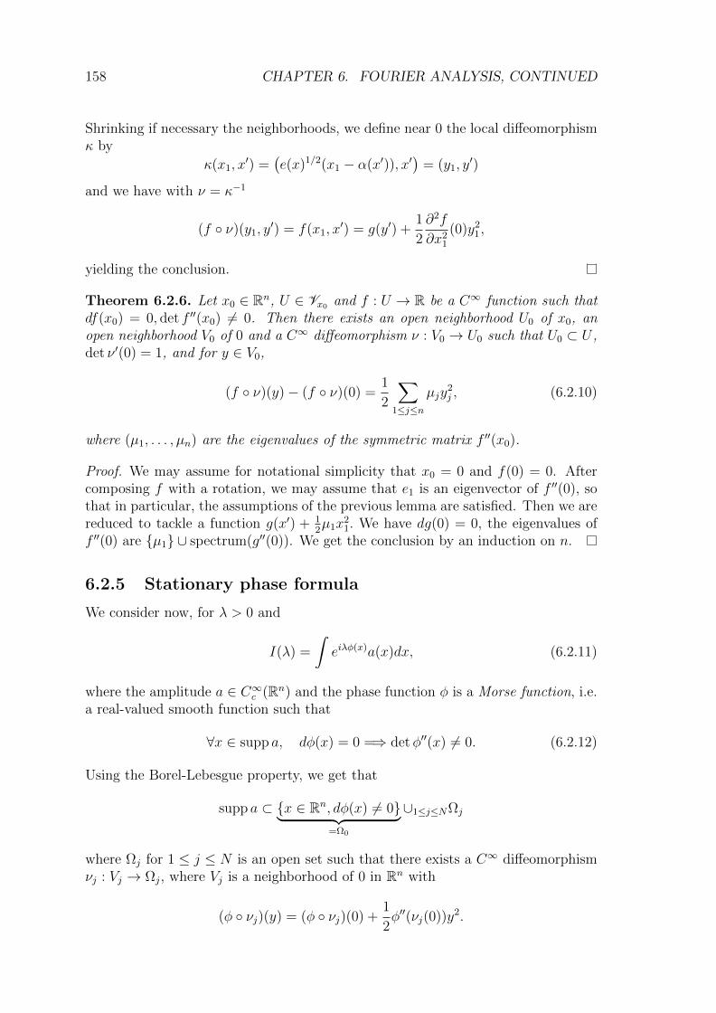
158 CHAPTER 6. FOURIER ANALYSIS, CONTINUED
Shrinking if necessary the neighborhoods, we define near 0 the local diffeomorphismκ by
κ(x1, x′) =
(e(x)1/2(x1 − α(x′)), x′
)= (y1, y
′)
and we have with ν = κ−1
(f ν)(y1, y′) = f(x1, x
′) = g(y′) +1
2
∂2f
∂x21
(0)y21,
yielding the conclusion.
Theorem 6.2.6. Let x0 ∈ Rn, U ∈ Vx0 and f : U → R be a C∞ function such thatdf(x0) = 0, det f ′′(x0) 6= 0. Then there exists an open neighborhood U0 of x0, anopen neighborhood V0 of 0 and a C∞ diffeomorphism ν : V0 → U0 such that U0 ⊂ U ,det ν ′(0) = 1, and for y ∈ V0,
(f ν)(y)− (f ν)(0) =1
2
∑1≤j≤n
µjy2j , (6.2.10)
where (µ1, . . . , µn) are the eigenvalues of the symmetric matrix f ′′(x0).
Proof. We may assume for notational simplicity that x0 = 0 and f(0) = 0. Aftercomposing f with a rotation, we may assume that e1 is an eigenvector of f ′′(0), sothat in particular, the assumptions of the previous lemma are satisfied. Then we arereduced to tackle a function g(x′) + 1
2µ1x
21. We have dg(0) = 0, the eigenvalues of
f ′′(0) are µ1 ∪ spectrum(g′′(0)). We get the conclusion by an induction on n.
6.2.5 Stationary phase formula
We consider now, for λ > 0 and
I(λ) =
∫eiλφ(x)a(x)dx, (6.2.11)
where the amplitude a ∈ C∞c (Rn) and the phase function φ is a Morse function, i.e.a real-valued smooth function such that
∀x ∈ supp a, dφ(x) = 0 =⇒ detφ′′(x) 6= 0. (6.2.12)
Using the Borel-Lebesgue property, we get that
supp a ⊂ x ∈ Rn, dφ(x) 6= 0︸ ︷︷ ︸=Ω0
∪1≤j≤NΩj
where Ωj for 1 ≤ j ≤ N is an open set such that there exists a C∞ diffeomorphismνj : Vj → Ωj, where Vj is a neighborhood of 0 in Rn with
(φ νj)(y) = (φ νj)(0) +1
2φ′′(νj(0))y2.
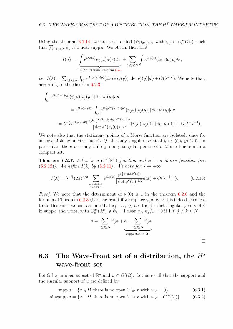
6.3. THEWAVE-FRONT SET OF ADISTRIBUTION, THEHS WAVE-FRONT SET159
Using the theorem 3.1.14, we are able to find (ψj)0≤j≤N with ψj ∈ C∞c (Ωj), suchthat
∑0≤j≤N ψj is 1 near supp a. We obtain then that
I(λ) =
∫eiλφ(x)ψ0(x)a(x)dx︸ ︷︷ ︸
=O(λ−∞) from Theorem 6.2.1
+∑
1≤j≤N
∫eiλφ(x)ψj(x)a(x)dx,
i.e. I(λ) =∑
1≤j≤N∫Vjeiλ(φνj)(y)(ψja)(νj(y))| det ν ′j(y)|dy +O(λ−∞). We note that,
according to the theorem 6.2.3∫Vj
eiλ(φνj)(y)(ψja)(νj(y))| det ν ′j(y)|dy
= eiλφ(νj(0))
∫Vj
eiλ12φ′′(νj(0))y2(ψja)(νj(y))| det ν ′j(y)|dy
= λ−n2 eiλφ(νj(0)) (2π)n/2ei
π4
signφ′′(νj(0))
| detφ′′(νj(0))|1/2(ψja)(νj(0))| det ν ′j(0)|+O(λ−
n2−1).
We note also that the stationary points of a Morse function are isolated, since foran invertible symmetric matrix Q, the only singular point of y 7→ 〈Qy, y〉 is 0. Inparticular, there are only finitely many singular points of a Morse function in acompact set.
Theorem 6.2.7. Let a be a C∞c (Rn) function and φ be a Morse function (see(6.2.12)). We define I(λ) by (6.2.11). We have for λ→ +∞
I(λ) = λ−n2 (2π)n/2
∑x,dφ(x)=0x∈supp a
eiλφ(x) eiπ4
sign(φ′′(x))
| detφ′′(x)|1/2a(x) +O(λ−
n2−1). (6.2.13)
Proof. We note that the determinant of ν ′(0) is 1 in the theorem 6.2.6 and theformula of Theorem 6.2.3 gives the result if we replace ψja by a; it is indeed harmlessto do this since we can assume that x1, . . . , xN are the distinct singular points of φin supp a and write, with C∞c (Rn) 3 ψj = 1 near xj, ψjψk = 0 if 1 ≤ j 6= k ≤ N
a =∑
1≤j≤N
ψja+ a−∑
1≤j≤N
ψja︸ ︷︷ ︸supported in Ω0
.
6.3 The Wave-Front set of a distribution, the Hs
wave-front set
Let Ω be an open subset of Rn and u ∈ D ′(Ω). Let us recall that the support andthe singular support of u are defined by
suppu = x ∈ Ω, there is no open V 3 x with u|V = 0, (6.3.1)
singsuppu = x ∈ Ω, there is no open V 3 x with u|V ∈ C∞(V ). (6.3.2)
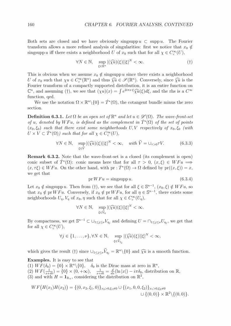
160 CHAPTER 6. FOURIER ANALYSIS, CONTINUED
Both sets are closed and we have obviously singsuppu ⊂ suppu. The Fouriertransform allows a more refined analysis of singularities: first we notice that x0 /∈singsuppu iff there exists a neighborhood U of x0 such that for all χ ∈ C∞c (U),
∀N ∈ N, supξ∈Rn|(χu)(ξ)||ξ|N <∞. (†)
This is obvious when we assume x0 /∈ singsuppu since there exists a neighborhoodU of x0 such that χu ∈ C∞c (Rn) and thus χu ∈ S (Rn). Conversely, since χu is theFourier transform of a compactly supported distribution, it is an entire function onCn, and assuming (†), we see that (χu)(x) =
∫e2iπx·ξχu(ξ)dξ, and the rhs is a C∞
function, qed.We use the notation Ω×Rn\0 = T ∗(Ω), the cotangent bundle minus the zero
section.
Definition 6.3.1. Let Ω be an open set of Rn and let u ∈ D ′(Ω). The wave-front-setof u, denoted by WFu, is defined as the complement in T ∗(Ω) of the set of points(x0, ξ0) such that there exist some neighborhoods U, V respectively of x0, ξ0 (withU × V ⊂ T ∗(Ω)) such that for all χ ∈ C∞c (U),
∀N ∈ N, supξ∈V|(χu)(ξ)||ξ|N <∞, with V = ∪τ>0τV. (6.3.3)
Remark 6.3.2. Note that the wave-front-set is a closed (its complement is open)conic subset of T ∗(Ω): conic means here that for all τ > 0, (x, ξ) ∈ WFu =⇒(x, τξ) ∈ WFu. On the other hand, with pr : T ∗(Ω)→ Ω defined by pr((x, ξ)) = x,we get that
prWFu = singsuppu. (6.3.4)
Let x0 /∈ singsuppu. Then from (†), we see that for all ξ ∈ Sn−1, (x0, ξ) /∈ WFu, sothat x0 /∈ prWFu. Conversely, if x0 /∈ prWFu, for all η ∈ Sn−1, there exists someneighborhoods Uη, Vη of x0, η such that for all χ ∈ C∞c (Uη),
∀N ∈ N, supξ∈Vη|(χu)(ξ)||ξ|N <∞.
By compactness, we get Sn−1 ⊂ ∪1≤j≤νVηj and defining U = ∩1≤j≤νUηj , we get thatfor all χ ∈ C∞c (U),
∀j ∈ 1, . . . , ν,∀N ∈ N, supξ∈Vηj
|(χu)(ξ)||ξ|N <∞,
which gives the result (†) since ∪1≤j≤νVηj = Rn\0 and χu is a smooth function.
Examples. It is easy to see that(1) WF (δ0) = 0 × Rn\0, δ0 is the Dirac mass at zero in Rn,(2) WF ( 1
x+i0) = 0 × (0,+∞), 1
x+i0= d
dx(ln |x|)− iπδ0, distribution on R,
(3) and with H = 1R+ , considering the distribution on R2,
WF(H(x1)H(x2)
)= (0, x2, ξ1, 0)x2>0,ξ1 6=0 ∪ (x1, 0, 0, ξ2)x1>0,ξ2 6=0
∪ (0, 0) × R2\(0, 0).
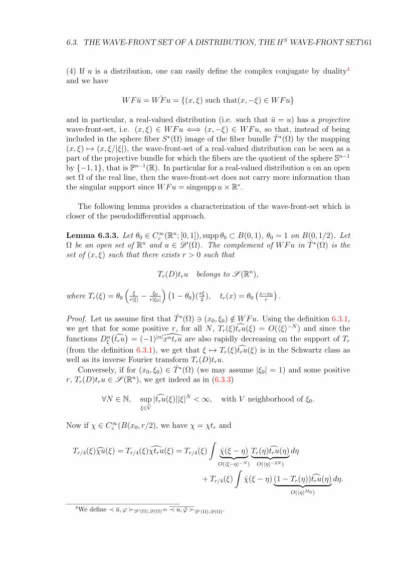
6.3. THEWAVE-FRONT SET OF ADISTRIBUTION, THEHS WAVE-FRONT SET161
(4) If u is a distribution, one can easily define the complex conjugate by duality4
and we have
WFu = ˇWFu = (x, ξ) such that(x,−ξ) ∈ WFu
and in particular, a real-valued distribution (i.e. such that u = u) has a projectivewave-front-set, i.e. (x, ξ) ∈ WFu ⇐⇒ (x,−ξ) ∈ WFu, so that, instead of beingincluded in the sphere fiber S∗(Ω) image of the fiber bundle T ∗(Ω) by the mapping(x, ξ) 7→ (x, ξ/|ξ|), the wave-front-set of a real-valued distribution can be seen as apart of the projective bundle for which the fibers are the quotient of the sphere Sn−1
by −1, 1, that is Pn−1(R). In particular for a real-valued distribution u on an openset Ω of the real line, then the wave-front-set does not carry more information thanthe singular support since WFu = singsuppu× R∗.
The following lemma provides a characterization of the wave-front-set which iscloser of the pseudodifferential approach.
Lemma 6.3.3. Let θ0 ∈ C∞c (Rn; [0, 1]), supp θ0 ⊂ B(0, 1), θ0 = 1 on B(0, 1/2). LetΩ be an open set of Rn and u ∈ D ′(Ω). The complement of WFu in T ∗(Ω) is theset of (x, ξ) such that there exists r > 0 such that
Tr(D)tru belongs to S (Rn),
where Tr(ξ) = θ0
(ξr|ξ| −
ξ0r|ξ0|
) (1− θ0
)( rξ
2), tr(x) = θ0
(x−x0r
).
Proof. Let us assume first that T ∗(Ω) 3 (x0, ξ0) /∈ WFu. Using the definition 6.3.1,we get that for some positive r, for all N , Tr(ξ)tru(ξ) = O(〈ξ〉−N) and since the
functions Dαξ
(tru)
= (−1)|α|xαtru are also rapidly decreasing on the support of Tr
(from the definition 6.3.1), we get that ξ 7→ Tr(ξ)tru(ξ) is in the Schwartz class aswell as its inverse Fourier transform Tr(D)tru.
Conversely, if for (x0, ξ0) ∈ T ∗(Ω) (we may assume |ξ0| = 1) and some positiver, Tr(D)tru ∈ S (Rn), we get indeed as in (6.3.3)
∀N ∈ N, supξ∈V|tru(ξ)||ξ|N <∞, with V neighborhood of ξ0.
Now if χ ∈ C∞c (B(x0, r/2), we have χ = χtr and
Tr/4(ξ)χu(ξ) = Tr/4(ξ)χtru(ξ) = Tr/4(ξ)
∫χ(ξ − η)︸ ︷︷ ︸O(〈ξ−η〉−N )
Tr(η)tru(η)︸ ︷︷ ︸O(〈η〉−2N )
dη
+ Tr/4(ξ)
∫χ(ξ − η) (1− Tr(η))tru(η)︸ ︷︷ ︸
O(〈η〉M0 )
dη.
4We define ≺ u, ϕ D′(Ω),D(Ω)= ≺ u, ϕ D′(Ω),D(Ω).
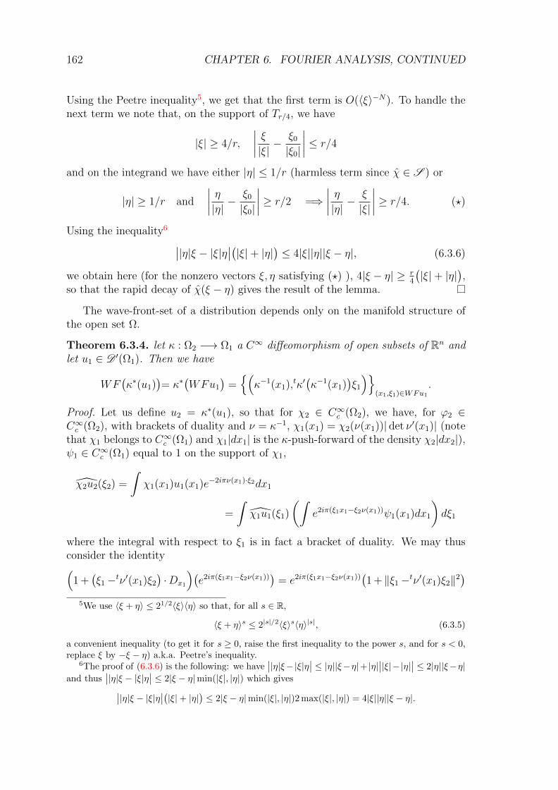
162 CHAPTER 6. FOURIER ANALYSIS, CONTINUED
Using the Peetre inequality5, we get that the first term is O(〈ξ〉−N). To handle thenext term we note that, on the support of Tr/4, we have
|ξ| ≥ 4/r,
∣∣∣∣ ξ|ξ| − ξ0
|ξ0|
∣∣∣∣ ≤ r/4
and on the integrand we have either |η| ≤ 1/r (harmless term since χ ∈ S ) or
|η| ≥ 1/r and
∣∣∣∣ η|η| − ξ0
|ξ0|
∣∣∣∣ ≥ r/2 =⇒∣∣∣∣ η|η| − ξ
|ξ|
∣∣∣∣ ≥ r/4. (?)
Using the inequality6 ∣∣|η|ξ − |ξ|η∣∣(|ξ|+ |η|) ≤ 4|ξ||η||ξ − η|, (6.3.6)
we obtain here (for the nonzero vectors ξ, η satisfying (?) ), 4|ξ − η| ≥ r4
(|ξ|+ |η|
),
so that the rapid decay of χ(ξ − η) gives the result of the lemma.
The wave-front-set of a distribution depends only on the manifold structure ofthe open set Ω.
Theorem 6.3.4. let κ : Ω2 −→ Ω1 a C∞ diffeomorphism of open subsets of Rn andlet u1 ∈ D ′(Ω1). Then we have
WF(κ∗(u1)
)= κ∗
(WFu1
)=(κ−1(x1),tκ′
(κ−1(x1)
)ξ1
)(x1,ξ1)∈WFu1
.
Proof. Let us define u2 = κ∗(u1), so that for χ2 ∈ C∞c (Ω2), we have, for ϕ2 ∈C∞c (Ω2), with brackets of duality and ν = κ−1, χ1(x1) = χ2(ν(x1))| det ν ′(x1)| (notethat χ1 belongs to C∞c (Ω1) and χ1|dx1| is the κ-push-forward of the density χ2|dx2|),ψ1 ∈ C∞c (Ω1) equal to 1 on the support of χ1,
χ2u2(ξ2) =
∫χ1(x1)u1(x1)e−2iπν(x1)·ξ2dx1
=
∫χ1u1(ξ1)
(∫e2iπ(ξ1x1−ξ2ν(x1))ψ1(x1)dx1
)dξ1
where the integral with respect to ξ1 is in fact a bracket of duality. We may thusconsider the identity(
1 +(ξ1−tν ′(x1)ξ2
)·Dx1
)(e2iπ(ξ1x1−ξ2ν(x1))
)= e2iπ(ξ1x1−ξ2ν(x1))
(1 + ‖ξ1−tν ′(x1)ξ2‖2
)5We use 〈ξ + η〉 ≤ 21/2〈ξ〉〈η〉 so that, for all s ∈ R,
〈ξ + η〉s ≤ 2|s|/2〈ξ〉s〈η〉|s|, (6.3.5)
a convenient inequality (to get it for s ≥ 0, raise the first inequality to the power s, and for s < 0,replace ξ by −ξ − η) a.k.a. Peetre’s inequality.
6The proof of (6.3.6) is the following: we have∣∣|η|ξ−|ξ|η∣∣ ≤ |η||ξ−η|+ |η|∣∣|ξ|−|η|∣∣ ≤ 2|η||ξ−η|
and thus∣∣|η|ξ − |ξ|η∣∣ ≤ 2|ξ − η|min(|ξ|, |η|) which gives∣∣|η|ξ − |ξ|η∣∣(|ξ|+ |η|) ≤ 2|ξ − η|min(|ξ|, |η|)2 max(|ξ|, |η|) = 4|ξ||η||ξ − η|.
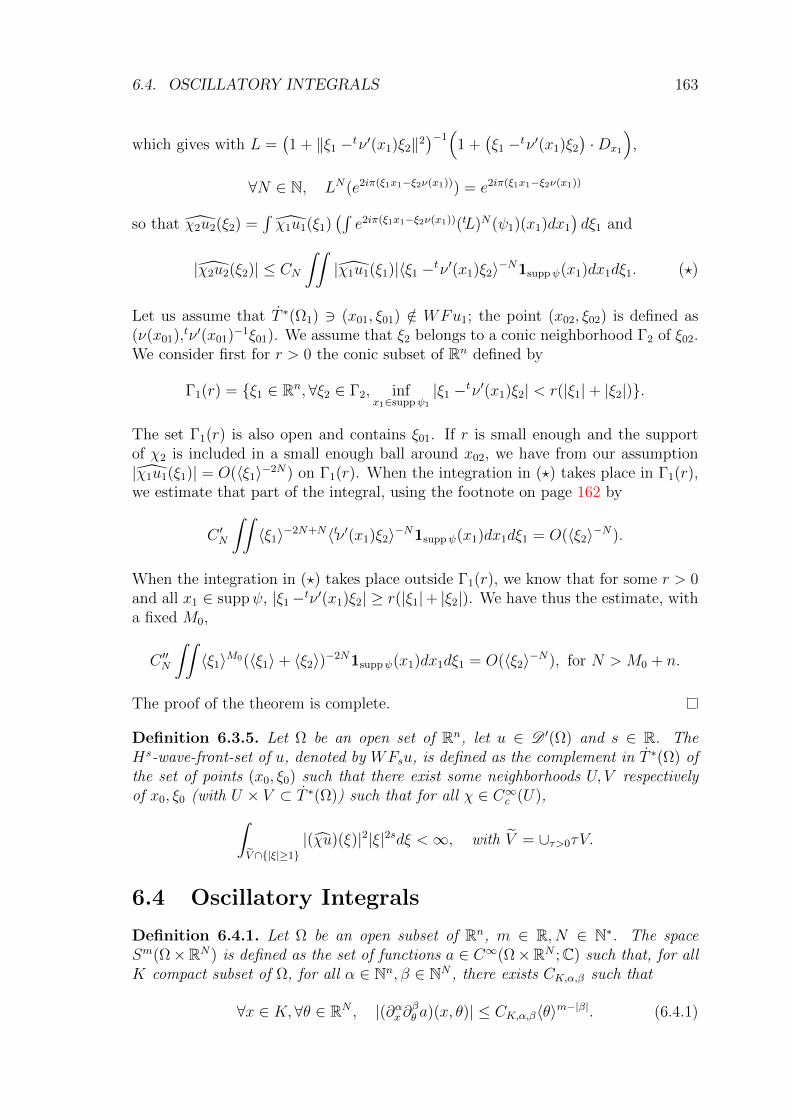
6.4. OSCILLATORY INTEGRALS 163
which gives with L =(1 + ‖ξ1 −tν ′(x1)ξ2‖2
)−1(
1 +(ξ1 −tν ′(x1)ξ2
)·Dx1
),
∀N ∈ N, LN(e2iπ(ξ1x1−ξ2ν(x1))) = e2iπ(ξ1x1−ξ2ν(x1))
so that χ2u2(ξ2) =∫χ1u1(ξ1)
(∫e2iπ(ξ1x1−ξ2ν(x1))(tL)N(ψ1)(x1)dx1
)dξ1 and
|χ2u2(ξ2)| ≤ CN
∫∫|χ1u1(ξ1)|〈ξ1 −tν ′(x1)ξ2〉−N1suppψ(x1)dx1dξ1. (?)
Let us assume that T ∗(Ω1) 3 (x01, ξ01) /∈ WFu1; the point (x02, ξ02) is defined as(ν(x01),tν ′(x01)−1ξ01). We assume that ξ2 belongs to a conic neighborhood Γ2 of ξ02.We consider first for r > 0 the conic subset of Rn defined by
Γ1(r) = ξ1 ∈ Rn,∀ξ2 ∈ Γ2, infx1∈suppψ1
|ξ1 −tν ′(x1)ξ2| < r(|ξ1|+ |ξ2|).
The set Γ1(r) is also open and contains ξ01. If r is small enough and the supportof χ2 is included in a small enough ball around x02, we have from our assumption|χ1u1(ξ1)| = O(〈ξ1〉−2N) on Γ1(r). When the integration in (?) takes place in Γ1(r),we estimate that part of the integral, using the footnote on page 162 by
C ′N
∫∫〈ξ1〉−2N+N〈tν ′(x1)ξ2〉−N1suppψ(x1)dx1dξ1 = O(〈ξ2〉−N).
When the integration in (?) takes place outside Γ1(r), we know that for some r > 0and all x1 ∈ suppψ, |ξ1−tν ′(x1)ξ2| ≥ r(|ξ1|+ |ξ2|). We have thus the estimate, witha fixed M0,
C ′′N
∫∫〈ξ1〉M0(〈ξ1〉+ 〈ξ2〉)−2N1suppψ(x1)dx1dξ1 = O(〈ξ2〉−N), for N > M0 + n.
The proof of the theorem is complete.
Definition 6.3.5. Let Ω be an open set of Rn, let u ∈ D ′(Ω) and s ∈ R. TheHs-wave-front-set of u, denoted by WFsu, is defined as the complement in T ∗(Ω) ofthe set of points (x0, ξ0) such that there exist some neighborhoods U, V respectivelyof x0, ξ0 (with U × V ⊂ T ∗(Ω)) such that for all χ ∈ C∞c (U),∫
V ∩|ξ|≥1|(χu)(ξ)|2|ξ|2sdξ <∞, with V = ∪τ>0τV.
6.4 Oscillatory Integrals
Definition 6.4.1. Let Ω be an open subset of Rn, m ∈ R, N ∈ N∗. The spaceSm(Ω×RN) is defined as the set of functions a ∈ C∞(Ω×RN ;C) such that, for allK compact subset of Ω, for all α ∈ Nn, β ∈ NN , there exists CK,α,β such that
∀x ∈ K, ∀θ ∈ RN , |(∂αx∂βθ a)(x, θ)| ≤ CK,α,β〈θ〉m−|β|. (6.4.1)
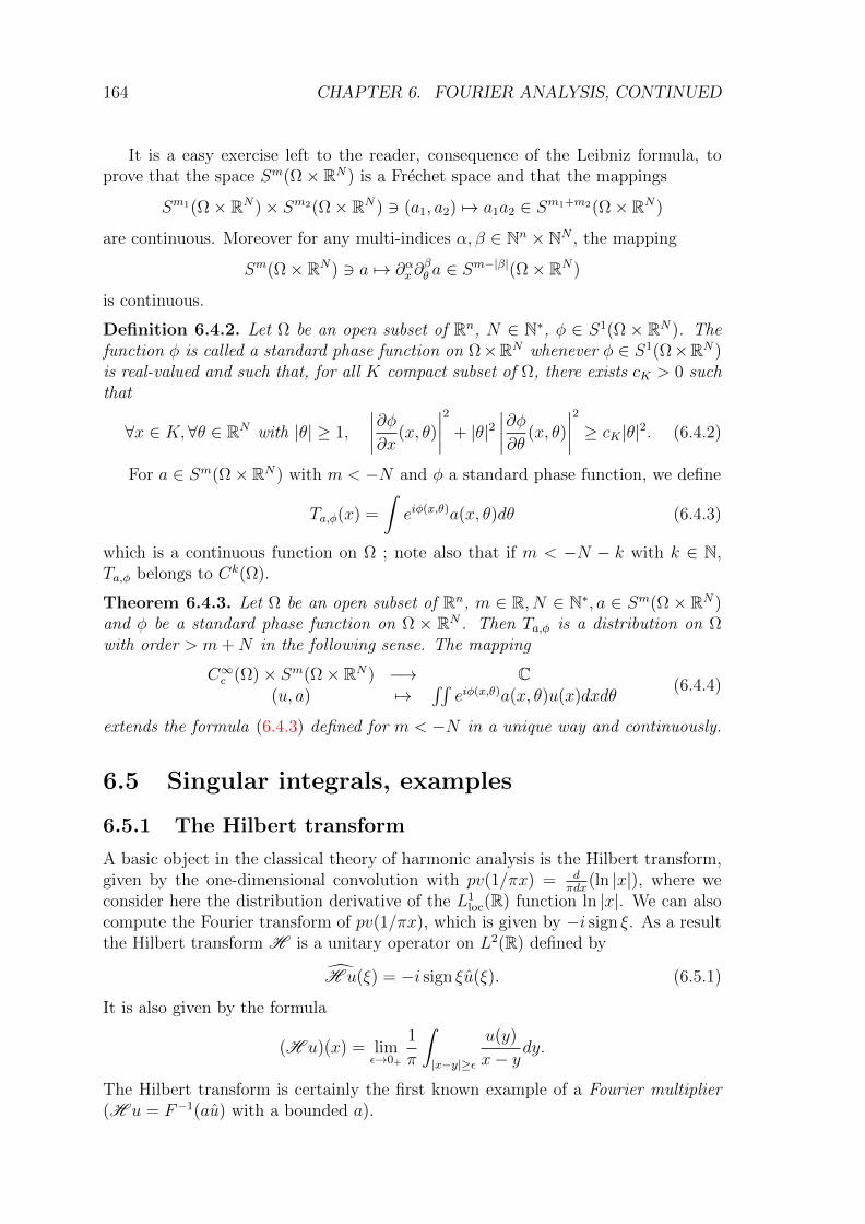
164 CHAPTER 6. FOURIER ANALYSIS, CONTINUED
It is a easy exercise left to the reader, consequence of the Leibniz formula, toprove that the space Sm(Ω× RN) is a Frechet space and that the mappings
Sm1(Ω× RN)× Sm2(Ω× RN) 3 (a1, a2) 7→ a1a2 ∈ Sm1+m2(Ω× RN)
are continuous. Moreover for any multi-indices α, β ∈ Nn × NN , the mapping
Sm(Ω× RN) 3 a 7→ ∂αx∂βθ a ∈ S
m−|β|(Ω× RN)
is continuous.
Definition 6.4.2. Let Ω be an open subset of Rn, N ∈ N∗, φ ∈ S1(Ω × RN). Thefunction φ is called a standard phase function on Ω×RN whenever φ ∈ S1(Ω×RN)is real-valued and such that, for all K compact subset of Ω, there exists cK > 0 suchthat
∀x ∈ K, ∀θ ∈ RN with |θ| ≥ 1,
∣∣∣∣∂φ∂x(x, θ)
∣∣∣∣2 + |θ|2∣∣∣∣∂φ∂θ (x, θ)
∣∣∣∣2 ≥ cK |θ|2. (6.4.2)
For a ∈ Sm(Ω× RN) with m < −N and φ a standard phase function, we define
Ta,φ(x) =
∫eiφ(x,θ)a(x, θ)dθ (6.4.3)
which is a continuous function on Ω ; note also that if m < −N − k with k ∈ N,Ta,φ belongs to Ck(Ω).
Theorem 6.4.3. Let Ω be an open subset of Rn, m ∈ R, N ∈ N∗, a ∈ Sm(Ω× RN)and φ be a standard phase function on Ω × RN . Then Ta,φ is a distribution on Ωwith order > m+N in the following sense. The mapping
C∞c (Ω)× Sm(Ω× RN) −→ C(u, a) 7→
∫∫eiφ(x,θ)a(x, θ)u(x)dxdθ
(6.4.4)
extends the formula (6.4.3) defined for m < −N in a unique way and continuously.
6.5 Singular integrals, examples
6.5.1 The Hilbert transform
A basic object in the classical theory of harmonic analysis is the Hilbert transform,given by the one-dimensional convolution with pv(1/πx) = d
πdx(ln |x|), where we
consider here the distribution derivative of the L1loc(R) function ln |x|. We can also
compute the Fourier transform of pv(1/πx), which is given by −i sign ξ. As a resultthe Hilbert transform H is a unitary operator on L2(R) defined by
H u(ξ) = −i sign ξu(ξ). (6.5.1)
It is also given by the formula
(H u)(x) = limε→0+
1
π
∫|x−y|≥ε
u(y)
x− ydy.
The Hilbert transform is certainly the first known example of a Fourier multiplier(H u = F−1(au) with a bounded a).
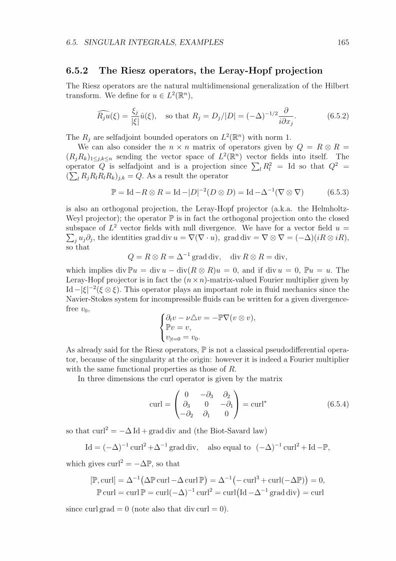
6.5. SINGULAR INTEGRALS, EXAMPLES 165
6.5.2 The Riesz operators, the Leray-Hopf projection
The Riesz operators are the natural multidimensional generalization of the Hilberttransform. We define for u ∈ L2(Rn),
Rju(ξ) =ξj|ξ|u(ξ), so that Rj = Dj/|D| = (−∆)−1/2 ∂
i∂xj. (6.5.2)
The Rj are selfadjoint bounded operators on L2(Rn) with norm 1.We can also consider the n × n matrix of operators given by Q = R ⊗ R =
(RjRk)1≤j,k≤n sending the vector space of L2(Rn) vector fields into itself. Theoperator Q is selfadjoint and is a projection since
∑lR
2l = Id so that Q2 =
(∑
lRjRlRlRk)j,k = Q. As a result the operator
P = Id−R⊗R = Id−|D|−2(D ⊗D) = Id−∆−1(∇⊗∇) (6.5.3)
is also an orthogonal projection, the Leray-Hopf projector (a.k.a. the Helmholtz-Weyl projector); the operator P is in fact the orthogonal projection onto the closedsubspace of L2 vector fields with null divergence. We have for a vector field u =∑
j uj∂j, the identities grad div u = ∇(∇ · u), grad div = ∇⊗∇ = (−∆)(iR⊗ iR),so that
Q = R⊗R = ∆−1 grad div, divR⊗R = div,
which implies divPu = div u − div(R ⊗ R)u = 0, and if div u = 0, Pu = u. TheLeray-Hopf projector is in fact the (n×n)-matrix-valued Fourier multiplier given byId−|ξ|−2(ξ ⊗ ξ). This operator plays an important role in fluid mechanics since theNavier-Stokes system for incompressible fluids can be written for a given divergence-free v0,
∂tv − ν4v = −P∇(v ⊗ v),Pv = v,v|t=0 = v0.
As already said for the Riesz operators, P is not a classical pseudodifferential opera-tor, because of the singularity at the origin: however it is indeed a Fourier multiplierwith the same functional properties as those of R.
In three dimensions the curl operator is given by the matrix
curl =
0 −∂3 ∂2
∂3 0 −∂1
−∂2 ∂1 0
= curl∗ (6.5.4)
so that curl2 = −∆ Id + grad div and (the Biot-Savard law)
Id = (−∆)−1 curl2 +∆−1 grad div, also equal to (−∆)−1 curl2 + Id−P,
which gives curl2 = −∆P, so that
[P, curl] = ∆−1(∆P curl−∆ curlP
)= ∆−1
(− curl3 + curl(−∆P)
)= 0,
P curl = curlP = curl(−∆)−1 curl2 = curl(Id−∆−1 grad div
)= curl
since curl grad = 0 (note also that div curl = 0).
166 CHAPTER 6. FOURIER ANALYSIS, CONTINUED
Theorem 6.5.1. Let Ω be a function in L1(Sn−1) such that∫Sn−1 Ω(ω)dσ(ω) = 0.
Then the following formula defines a tempered distribution T :
〈T, ϕ〉 = limε→0+
∫|x|≥ε
Ω( x|x|)|x|−nϕ(x)dx = −
∫(x · ∂xϕ(x))Ω
( x|x|)|x|−n ln |x|dx.
The distribution T is homogeneous of degree −n on Rn and, if Ω is odd, the Fouriertransform of T is a bounded function.
N.B. We shall use the principal-value notation
T = pv(|x|−nΩ
( x|x|)).
When n = 1 and Ω = sign, we recover the principal value pv(1/x) = ddx
(ln |x|) whichis odd, homogeneous of degree -1, and whose Fourier transform is −iπ sign ξ.
Proof. Let ϕ be in S (Rn) and ε > 0. Using polar coordinates, we check∫Sn−1
Ω(ω)
∫ +∞
ε
ϕ(rω)dr
rdσ(ω)
=
∫Sn−1
Ω(ω)[ϕ(εω) ln(ε−1)−
∫ +∞
ε
ω · dϕ(rω) ln rdr]dσ(ω).
Since the mean value of Ω is 0, we get the first statement of the theorem, noticingthat the function x 7→ Ω(x/|x|)|x|−n+1 ln(|x|)(1 + |x|)−2 is in L1(Rn). We have
〈x · ∂xT, ϕ〉 = −〈T, x · ∂xϕ〉 − n〈T, ϕ〉 (~)
and we see that
〈T, x · ∂xϕ〉 = limε→0+
∫Sn−1
Ω(ω)
∫ +∞
ε
rω · (dϕ)(rω)dr
rdσ(ω)
=
∫Sn−1
Ω(ω)
∫ +∞
0
ω · (dϕ)(rω)drdσ(ω)
=
∫Sn−1
Ω(ω)
∫ +∞
0
d
dr
(ϕ(rω)
)drdσ(ω) = −ϕ(0)
∫Sn−1
Ω(ω)dσ(ω) = 0
so that (~) implies that x ·∂xT = −nT which is the homogeneity of degree −n of T .As a result the Fourier transform of T is an homogeneous distribution with degree0.
N.B. Note that the formula
−∫
(x · ∂xϕ(x))Ω( x|x|)|x|−n ln |x|dx
makes sense for Ω ∈ L1(Sn−1), ϕ ∈ S (Rn) and defines a tempered distribution. Forinstance, if n = 1 and Ω = 1, we get the distribution derivative d
dx
(signx ln |x|
).
However, the condition of mean value 0 for Ω on the sphere is necessary to obtain T
6.6. APPENDIX 167
as a principal value, since in the discussion above, the term factored out by ln(1/ε)is∫Sn−1 Ω(ω)ϕ(εω)dσ(ω) which has the limit ϕ(0)
∫Sn−1 Ω(ω)dσ(ω). On the other
hand, from the defining formula of T , we get with Ωj(ω) = 12(Ω(ω) + (−1)jΩ(−ω))
(Ω1(resp.Ω2) is the odd (resp. even) part of Ω)
〈T, ϕ〉 =
∫Sn−1
Ω1(ω)〈pv(1
2t), ϕ(tω)〉S ′(Rt),S (Rt)dσ(ω)
+
∫Sn−1
Ω2(ω)〈 ddt
(H(t) ln t
), ϕ(tω)〉S ′(Rt),S (Rt)dσ(ω). (6.5.5)
Let us show that, when Ω is odd, the Fourier transform of T is bounded. We get
〈T , ψ〉 =
∫Sn−1
Ω(ω)〈pv(1
2t), ψ(tω)〉dσ(ω)
= −iπ2
∫Rn
∫Sn−1
Ω(ω) sign(ω · ξ)ϕ(ξ)dξdσ(ω)
proving that
T (ξ) = −iπ2
∫Sn−1
Ω(ω) sign(ω · ξ)dσ(ω) (6.5.6)
which is indeed a bounded function.
6.6 Appendix
6.6.1 On the Faa di Bruno formula
That formula7 is dealing with the iterated derivative of a composition of functions.First of all, let us consider (smooth) functions of one real variable
Uf−→ V
g−→ W, U, V,W open sets of R.
With g(r) always evaluated at f(x), we have
(g f)′ = g′f ′
(g f)′′ = g′′f ′2 + g′f ′′
(g f)′′′ = g′′′f ′3 + g′′3f ′′f ′ + g′f ′′′
(g f)(4) = g(4)(f ′)4 + 6g(3)f ′2f ′′ + g′′(4f ′′′f ′ + 3f ′′
2) + g′f (4)
i.e.1
4!(g f)(4) =
g(4)
4!
(f ′
1!
)4
+ 3g(3)
3!
(f ′′
2!
)(f ′
1!
)2
+g(2)
2!
[(f ′′2!
)2
+ 2f ′′′
3!f ′]
+g(1)
1!
f (4)
4!.
7Francesco Faa di Bruno (1825–1888) was an italian mathematician and priest, born at Alessan-dria. He was beatified in 1988, probably the only mathematician to reach sainthood so far. The“Chevalier Francois Faa di Bruno, Capitaine honoraire d’Etat-Major dans l’armee Sarde”, defendedhis thesis in 1856, in the Faculte des Sciences de Paris in front of the following jury: Cauchy (chair),Lame and Delaunay.
168 CHAPTER 6. FOURIER ANALYSIS, CONTINUED
More generally we have the remarkably simple
(g f)(k)
k!=∑
1≤r≤k
g(r) fr!
∏k1+···+kr=k
kj≥1
f (kj)
kj!. (6.6.1)
· There is only one multi-index (1, 1, 1, 1) ∈ N∗4 such that∑
1≤j≤4 kj = 4.
· There are 3 multi-indices (1, 1, 2), (1, 2, 1), (2, 1, 1) ∈ N∗3 with∑
1≤j≤3 kj = 4.
· There is 1 multi-index (2, 2) ∈ N∗2 with∑
1≤j≤2 kj = 4 and 2 multiindices(1, 3), (3, 1) such that
∑1≤j≤2 kj = 4.
· There is 1 index 4 ∈ N∗ with∑
1≤j≤1 kj = 4.Usually the formula is written in a different way with the more complicated
(g f)(k)
k!=
∑l1+2l2+···+klk=k
r=l1+···+lk
g(r) fl1! . . . lk!
∏1≤j≤k
(f (j)
j!
)lj. (6.6.2)
Let us show that the two formulas coincide. We start from (6.6.1)
(g f)(k)
k!=∑
1≤r≤k
g(r) fr!
∏k1+···+kr=k
kj≥1
f (kj)
kj!.
If we consider a multi-index
(k1, . . . , kr) = (1, . . . , 1︸ ︷︷ ︸l1times
, 2, . . . , 2︸ ︷︷ ︸l2times
, . . . , j, . . . , j,︸ ︷︷ ︸ljtimes
. . . , k, . . . , k︸ ︷︷ ︸lktimes
)
we get in factor of g(r)/r! the term∏
1≤j≤k
(f (j)
j!
)ljwith l1 + 2l2 + · · · + klk =
k, l1 + · · ·+ lk = r and since we can permute the (k1, . . . , kr) above, we get indeeda factor r!
l1!...lk!which gives (6.6.2).
The proof above can easily be generalized to a multidimensional setting with
Uf−→ V
g−→ W, U, V,W open sets of Rm,Rn,Rp, f, g of class Ck.
Since the derivatives are multilinear symmetric mappings, they are completely de-termined by their values on the “diagonal” T ⊗ · · · ⊗ T : the symmetrized productsof T1 ⊗ · · · ⊗ Tk, noted as T1 . . . Tk, can be written as a linear combination of k-thpowers. In fact, in a commutative algebra on a field with characteristic 0, using thepolarization formula, the products T1 . . . Tk are linear combination of k-th powers
T1T2 . . . Tk =1
2kk!
∑εj=±1
ε1 . . . εk(ε1T1 + · · ·+ εkTk)k. (6.6.3)
For T ∈ Tx(U), we have
(g f)(k)
k!T k =
∑1≤r≤k
g(r) fr!
∏k1+···+kr=k
kj≥1
f (kj)
kj!T kj ,
which is consistent with the fact that f (kj)(x)T kj belongs to the tangent spaceTf(x)(V ) of V at f(x) and ⊗1≤j≤rf
(kj)(x)T kj is a tensor product in T r,0(Tf(x)(V )) onwhich g(r)(f(x)) acts to send it on Tg(f(x))(W ).
Bibliography
[1] N. Bourbaki, Elements de mathematique. Topologie generale. Chapitres 1 a 4,Hermann, Paris, 1971. MR MR0358652 (50 #11111)
[2] , Elements de mathematique, Hermann, Paris, 1976, Fonctions d’unevariable reelle, Theorie elementaire, Nouvelle edition. MR MR0580296 (58#28327)
[3] H. Brezis, Analyse fonctionnelle, Masson, 1983.
[4] Gustave Choquet, Topology, Translated from the French by Amiel Feinstein.Pure and Applied Mathematics, Vol. XIX, Academic Press, New York, 1966.MR MR0193605 (33 #1823)
[5] John B. Conway, A course in functional analysis, second ed., Graduate Textsin Mathematics, vol. 96, Springer-Verlag, New York, 1990. MR MR1070713(91e:46001)
[6] F.G. Friedlander, Introduction to the theory of distributions, Cambridge Uni-versity Press, 1982.
[7] L. Hormander, The analysis of linear partial differential operators, Springer-Verlag, 1983.
[8] Michael T. Lacey, Carleson’s theorem: proof, complements, variations, Publ.Mat. 48 (2004), no. 2, 251–307. MR MR2091007 (2005e:42020)
[9] N. Lerner, Integration, http://www.math.jussieu.fr/lerner/int.nte.html, 2000.
[10] University of St Andrews, History of mathematics, http://www-history.mcs.st-and.ac.uk/history/, .
[11] Michael Reed and Barry Simon, Methods of modern mathematical physics. I,second ed., Academic Press Inc. [Harcourt Brace Jovanovich Publishers], NewYork, 1980, Functional analysis. MR MR751959 (85e:46002)
[12] W. Rudin, Real and complex analysis, McGraw-hill, 1966.
[13] , Functional analysis, McGraw-hill, 1973.
[14] F. Treves, Topological vector spaces, distributions and kernels, Academic Press,1967.
169
Index
NotationsDxj = 1
2iπ∂∂xj
, 102
Log: the principal determination ofthe logarithm in C\R−, 124
Υ+: the n × n complex nonsingularsymmetric matrices with nonneg-ative real part, 124
Υ∗+: the n × n complex symmetricmatrices with a positive definitereal part, 125
Fourier inversion formula, 102Fourier transform, 101
Schwartz, 101
170

![arxiv.org · arXiv:1510.05230v1 [math.CV] 18 Oct 2015 Extension of holomorphic functions defined on non reduced analytic subvarieties Jean-Pierre Demailly Institut Fourier, Universit´e](https://img.pdfslide.net/doc/110x75/5f085b3f7e708231d4219b07/arxivorg-arxiv151005230v1-mathcv-18-oct-2015-extension-of-holomorphic-functions.jpg)


![arxiv.org · arXiv:1512.03503v2 [cs.SC] 13 Jun 2016 Computingminimal interpolationbases Claude-Pierre Jeannerod Inria, Universit´e de Lyon Laboratoire LIP (CNRS, Inria, ENS de Lyon,](https://img.pdfslide.net/doc/110x75/605719f5b36ed940396d020e/arxivorg-arxiv151203503v2-cssc-13-jun-2016-computingminimal-interpolationbases.jpg)