Lecture notes on several complexvariables

Harold P. BoasDraft of December 3, 2013

Contents

1 Introduction 11.1 Power series . . . . . . . . . . . . . . . . . . . . . . . . . . . . . . . . . . . . . 21.2 Integral representations . . . . . . . . . . . . . . . . . . . . . . . . . . . . . . . 31.3 Partial differential equations . . . . . . . . . . . . . . . . . . . . . . . . . . . . 31.4 Geometry . . . . . . . . . . . . . . . . . . . . . . . . . . . . . . . . . . . . . . 4

2 Power series 62.1 Domain of convergence . . . . . . . . . . . . . . . . . . . . . . . . . . . . . . . 62.2 Characterization of domains of convergence . . . . . . . . . . . . . . . . . . . . 72.3 Elementary properties of holomorphic functions . . . . . . . . . . . . . . . . . . 112.4 The Hartogs phenomenon . . . . . . . . . . . . . . . . . . . . . . . . . . . . . . 122.5 Natural boundaries . . . . . . . . . . . . . . . . . . . . . . . . . . . . . . . . . 142.6 Summary: domains of convergence . . . . . . . . . . . . . . . . . . . . . . . . 222.7 Separate holomorphicity implies joint holomorphicity . . . . . . . . . . . . . . . 23

3 Holomorphic mappings 273.1 Fatou–Bieberbach domains . . . . . . . . . . . . . . . . . . . . . . . . . . . . . 27

3.1.1 Example . . . . . . . . . . . . . . . . . . . . . . . . . . . . . . . . . . 283.1.2 Theorem . . . . . . . . . . . . . . . . . . . . . . . . . . . . . . . . . . 30

3.2 Inequivalence of the ball and the bidisc . . . . . . . . . . . . . . . . . . . . . . 313.3 Injectivity and the Jacobian . . . . . . . . . . . . . . . . . . . . . . . . . . . . . 323.4 The Jacobian conjecture . . . . . . . . . . . . . . . . . . . . . . . . . . . . . . 35

4 Convexity 374.1 Real convexity . . . . . . . . . . . . . . . . . . . . . . . . . . . . . . . . . . . . 374.2 Convexity with respect to a class of functions . . . . . . . . . . . . . . . . . . . 38

4.2.1 Polynomial convexity . . . . . . . . . . . . . . . . . . . . . . . . . . . . 394.2.2 Linear and rational convexity . . . . . . . . . . . . . . . . . . . . . . . . 444.2.3 Holomorphic convexity . . . . . . . . . . . . . . . . . . . . . . . . . . . 474.2.4 Pseudoconvexity . . . . . . . . . . . . . . . . . . . . . . . . . . . . . . 56

4.3 The Levi problem . . . . . . . . . . . . . . . . . . . . . . . . . . . . . . . . . . 664.3.1 The Levi form . . . . . . . . . . . . . . . . . . . . . . . . . . . . . . . 674.3.2 Applications of the ) problem . . . . . . . . . . . . . . . . . . . . . . . 704.3.3 Solution of the )-equation on smooth pseudoconvex domains . . . . . . . 75

ii

1 Introduction

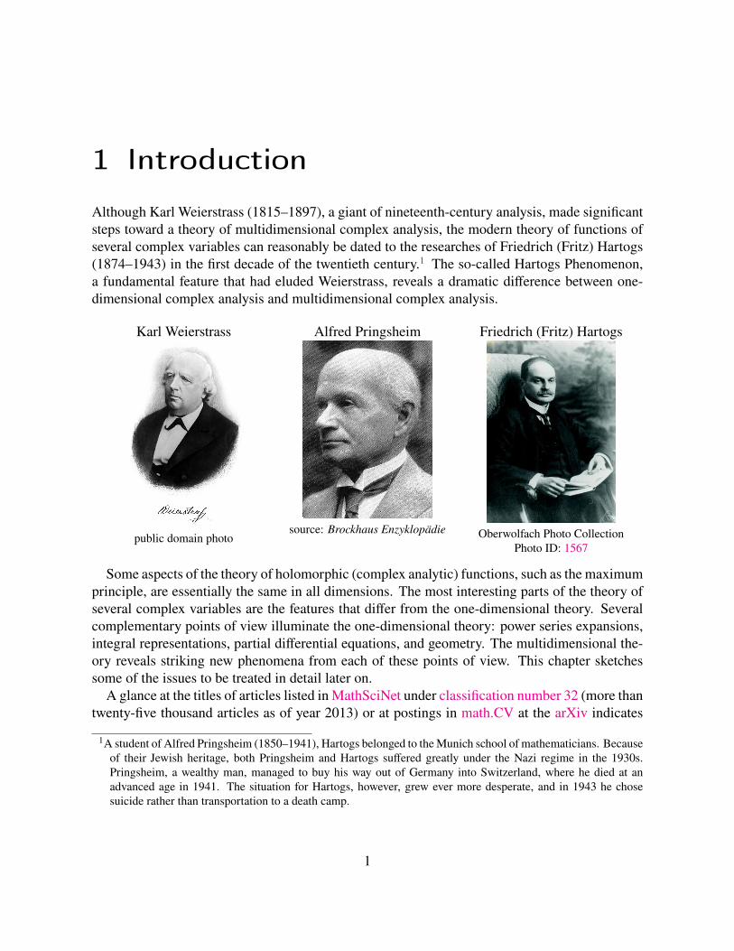
Although Karl Weierstrass (1815–1897), a giant of nineteenth-century analysis, made significantsteps toward a theory of multidimensional complex analysis, the modern theory of functions ofseveral complex variables can reasonably be dated to the researches of Friedrich (Fritz) Hartogs(1874–1943) in the first decade of the twentieth century.1 The so-called Hartogs Phenomenon,a fundamental feature that had eluded Weierstrass, reveals a dramatic difference between one-dimensional complex analysis and multidimensional complex analysis.

Karl Weierstrass

public domain photo

Alfred Pringsheim

source: Brockhaus Enzyklopädie

Friedrich (Fritz) Hartogs

Oberwolfach Photo CollectionPhoto ID: 1567

Some aspects of the theory of holomorphic (complex analytic) functions, such as the maximumprinciple, are essentially the same in all dimensions. The most interesting parts of the theory ofseveral complex variables are the features that differ from the one-dimensional theory. Severalcomplementary points of view illuminate the one-dimensional theory: power series expansions,integral representations, partial differential equations, and geometry. The multidimensional the-ory reveals striking new phenomena from each of these points of view. This chapter sketchessome of the issues to be treated in detail later on.

A glance at the titles of articles listed in MathSciNet under classification number 32 (more thantwenty-five thousand articles as of year 2013) or at postings in math.CV at the arXiv indicates1A student of Alfred Pringsheim (1850–1941), Hartogs belonged to theMunich school of mathematicians. Becauseof their Jewish heritage, both Pringsheim and Hartogs suffered greatly under the Nazi regime in the 1930s.Pringsheim, a wealthy man, managed to buy his way out of Germany into Switzerland, where he died at anadvanced age in 1941. The situation for Hartogs, however, grew ever more desperate, and in 1943 he chosesuicide rather than transportation to a death camp.

1

1 Introduction

the scope of the interaction between complex analysis and other parts of mathematics, includinggeometry, partial differential equations, probability, functional analysis, algebra, and mathemat-ical physics. One of the goals of this course is to glimpse some of these connections betweendifferent areas of mathematics.

1.1 Power series

A power series in one complex variable converges absolutely inside a certain disc and divergesoutside the closure of the disc. But the convergence region for a power series in two (or more)variables can have infinitely many different shapes. For instance, the largest open set in whichthe double series ∑∞

n=0∑∞

m=0 zn1zm2 converges absolutely is the unit bidisc { (z1, z2) ∶ |z1| < 1

and |z2| < 1 }, while the series ∑∞n=0 z

n1zn2 converges in the unbounded hyperbolic region where

|z1z2| < 1.The theory of one-dimensional power series bifurcates into the theory of entire functions (whenthe series has infinite radius of convergence) and the theory of holomorphic functions on theunit disc (when the series has a finite radius of convergence—which can be normalized to thevalue 1). In higher dimensions, the study of power series leads to function theory on infinitelymany different types of domains. A natural problem, to be solved later, is to characterize thedomains that are convergence domains for multivariable power series.Exercise 1. Find a concrete power series whose convergence domain is the two-dimensional unitball { (z1, z2) ∶ |z1|2 + |z2|2 < 1 }.While studying series, Hartogs discovered that every function holomorphic in a neighborhood

of the boundary of the unit bidisc automatically extends to be holomorphic on the interior of thebidisc; a proof can be carried out by considering one-variable Laurent series on slices. Thus,in dramatic contrast to the situation in one variable, there are domains in ℂ2 on which all theholomorphic functions extend to a larger domain. A natural question, to be answered later, is tocharacterize the domains of holomorphy, that is, the natural domains of existence of holomorphicfunctions.

The discovery of Hartogs shows too that holomorphic functions of several variables neverhave isolated singularities and never have isolated zeroes, in contrast to the one-variable case.Moreover, zeroes (and singularities) must propagate either to infinity or to the boundary of thedomain where the function is defined.Exercise 2. Let p(z1, z2) be a nonconstant polynomial in two complex variables. Show that thezero set of p cannot be a compact subset of ℂ2.

2

1 Introduction

1.2 Integral representations

The one-variable Cauchy integral formula for a holomorphic function f on a domain bounded bya simple closed curve C says that

f (z) = 12�i ∫C

f (w)w − z

dw for z inside C.

A remarkable feature of this formula is that the kernel (w − z)−1 is both universal (independentof the curve C) and holomorphic in the free variable z. There is no such formula in higherdimensions! There are integral representations with a holomorphic kernel that depends on thedomain, and there is a universal integral representation with a kernel that is not holomorphic. Ahuge literature addresses the problem of constructing and analyzing integral representations forvarious special types of domains.

There is an iterated Cauchy integral formula: namely,

f (z1, z2) =( 12�i

)2

∫C1 ∫C2

f (w1, w2)(w1 − z1)(w2 − z2)

dw1 dw2

for z1 in the regionD1 bounded by the simple closed curve C1 and z2 in the regionD2 bounded bythe simple closed curve C2. But this formula is special to a product domain D1 ×D2. Moreover,the integration here is over only a small portion of the boundary of the region, for the set C1 ×C2has real dimension 2, while the boundary of D1 ×D2 has real dimension 3. The iterated Cauchyintegral is important and useful within its limited realm of applicability.

1.3 Partial differential equations

The one-dimensional Cauchy–Riemann equations are two real partial differential equations fortwo functions (the real part and the imaginary part of a holomorphic function). In ℂn, thereare still two functions, but there are 2n equations. When n > 1, the inhomogeneous Cauchy–Riemann equations form an overdetermined system; there is a necessary compatibility conditionfor solvability of the Cauchy–Riemann equations. This feature is a significant difference from theone-variable theory.

When the inhomogeneous Cauchy–Riemann equations are solvable in ℂ2 (or in higher dimen-sions), there is (as will be shown later) a solution with compact support in the case of compactlysupported data. When n = 1, however, it is not always possible to solve the inhomogeneousCauchy–Riemann equations while maintaining compact support. The Hartogs phenomenon canbe interpreted as one manifestation of this dimensional difference.Exercise 3. Show that if u is the real part of a holomorphic function of two complex variablesz1 (= x1 + iy1) and z2 (= x2 + iy2), then the function u must satisfy the following system of real

3

1 Introduction

second-order partial differential equations:)2u)x21

+ )2u)y21

= 0, )2u)x1)x2

+ )2u)y1)y2

= 0,

)2u)x22

+ )2u)y22

= 0, )2u)x1)y2

− )2u)y1)x2

= 0.

Thus the real part of a holomorphic function of two variables not only is harmonic in each coor-dinate but also satisfies additional conditions.

1.4 Geometry

In view of the one-variable Riemann mapping theorem, every bounded simply connected planardomain is biholomorphically equivalent to the unit disc. In higher dimension, there is no suchsimple topological classification of biholomorphically equivalent domains. Indeed, the unit ballinℂ2 and the unit bidisc inℂ2 are holomorphically inequivalent domains (as will be proved later).

An intuitive way to understand why the situation changes in dimension 2 is to realize thatin ℂ2, there is room for one-dimensional complex analysis to happen in the tangent space to theboundary of a domain. Indeed, the boundary of the bidisc contains pieces of one-dimensionalaffine complex subspaces, while the boundary of the two-dimensional ball does not contain anynontrivial analytic disc (the image of the unit disc under a holomorphic mapping).

Similarly, there is room for complex analysis to happen inside the zero set of a holomorphicfunction from ℂ2 to ℂ1. The zero set of a function such as z1z2 is a one-dimensional complexvariety inside ℂ2, while the zero set of a nontrivial holomorphic function from ℂ1 to ℂ1 is azero-dimensional variety (that is, a discrete set of points).

Notice that there is a mismatch between the dimension of the domain and the dimension of therange of a multivariable holomorphic function. Accordingly, one might expect the right analogueof a holomorphic function from ℂ1 to ℂ1 to be an equidimensional holomorphic mapping fromℂn to ℂn. But here too there are surprises.

First of all, notice that a biholomorphic mapping in dimension 2 (or higher) need not be aconformal (angle-preserving) map.2 Indeed, even a linear transformation of ℂ2, such as the mapsending (z1, z2) to (z1 + z2, z2), can change the angles at which lines meet. Although conformalmaps are plentiful in the setting of one complex variable, conformality is a quite rigid propertyin higher dimensions. Indeed, a theorem of Joseph Liouville (1809–1882) states3 that the only2Biholomorphic mappings used to be called “pseudoconformal” mappings, but this word has gone out of fashion.3In 1850, Liouville published a fifth edition of Application de l’analyse à la géométrie by Gaspard Monge (1746–1818). An appendix includes seven long notes by Liouville. The sixth of these notes, bearing the title “Extensionau cas des trois dimensions de la question du tracé géographique” and extending over pages 609–616, containsthe proof of the theorem in dimension 3.Two sources for modern treatments of this theorem are Chapters 5–6 of David E. Blair’s Inversion Theory

and Conformal Mapping [American Mathematical Society, 2000]; and Theorem 5.2 of Chapter 8 of ManfredoPerdigão do Carmo’s Riemannian Geometry [Birkhäuser, 1992].

4

1 Introduction

conformal mappings from a domain in ℝn into ℝn (where n ≥ 3) are the (restrictions of) Möbiustransformations: compositions of translations, dilations, orthogonal linear transformations, andinversions.

Remarkably, there exists a biholomorphic mapping from all of ℂ2 onto a proper subset of ℂ2

whose complement has interior points. Such a mapping is called a Fatou–Bieberbach map.4

4The name honors the French mathematician Pierre Fatou (1878–1929), known also for the Fatou lemma in thetheory of the Lebesgue integral; and theGermanmathematician Ludwig Bieberbach (1886–1982), known also forthe Bieberbach Conjecture about schlicht functions (solved by Louis de Branges around 1984), for contributionsto the theory of crystallographic groups, and—infamously—for being an enthusiastic Nazi.

5

2 Power series

Examples in the introduction show that the domain of convergence of a multivariable power seriescan have a variety of shapes; in particular, the domain of convergence need not be a convex set.Nonetheless, there is a special kind of convexity property that characterizes convergence domains.

Developing the theory requires some notation. The Cartesian product of n copies of the com-plex numbers ℂ is denoted by ℂn. In contrast to the one-dimensional case, the space ℂn is notan algebra when n > 1 (there is no multiplication operation). But the space ℂn is a normedvector space, the usual norm being the Euclidean one: ‖(z1,… , zn)‖2 =

√

|z1|2 +⋯ + |zn|2. Apoint (z1,… , zn) in ℂn is commonly denoted by a single letter z, a vector variable. If � is an n-dimensional vector all of whose coordinates are nonnegative integers, then z� means the productz�11 ⋯ z�nn (as usual, the quantity z�11 is interpreted as 1 when z1 and �1 are simultaneously equalto 0); the notation �! abbreviates the product �1!⋯ �n! (where 0! = 1); and |�|means �1+⋯+�n.In this “multi-index” notation, a multivariable power series can be written in the form ∑

� c�z�,an abbreviation for∑∞�1=0

⋯∑∞

�n=0c�1,…,�nz

�11 ⋯ z�nn .

There is some awkwardness in talking about convergence of a multivariable power series∑

� c�z�, because the value of a series depends (in general) on the order of summation, and thereis no canonical ordering of n-tuples of nonnegative integers when n > 1.Exercise 4. Find complex numbers b� such that the “triangular” sum limk→∞

∑kj=0

∑

|�|=j b� andthe “square” sum limk→∞

∑k�1=0

⋯∑k

�n=0b� have different finite values.

Accordingly, it is convenient to restrict attention to absolute convergence, since the terms of anabsolutely convergent series can be reordered arbitrarily without changing the value of the sum(or the convergence of the sum).

2.1 Domain of convergence

The domain of convergence of a power series means the interior of the set of points at which theseries converges absolutely. For example, the power series ∑∞

n=1 zn1zn!2 converges absolutely on

the union of three sets in ℂ2: the points (z1, z2) for which |z2| < 1 and z1 is arbitrary; the points(0, z2) for arbitrary z2; and the points (z1, z2) for which |z2| = 1 and |z1| < 1. The domain ofconvergence is the first of these three sets, for the other two sets contribute no additional interiorpoints.

Being defined by absolute convergence, every convergence domain is multicircular: if a point(z1,… , zn) lies in the domain, then so does the point (�1z1,… , �nzn) when 1 = |�1| = ⋯ =|�n|. Moreover, the comparison test for absolute convergence of series shows that the point

6

2 Power series

(�1z1,… , �nzn) remains in the convergence domain when |�j| ≤ 1 for each j. Thus every con-vergence domain is a union of polydiscs centered at the origin. (A polydisc means a Cartesianproduct of discs, possibly with different radii.)

A multicircular domain is often called a Reinhardt domain.1 Such a domain is called completeif whenever a point z lies in the domain, the whole polydisc {w ∶ |w1| ≤ |z1|,… , |wn| ≤ |zn| }is contained in the domain. The preceding discussion can be rephrased as saying that everyconvergence domain is a complete Reinhardt domain.

But more is true. If both ∑� |c�z�| and∑

� |c�w�| converge, then Hölder’s inequality implies

that ∑� |c�||z�|t|w�|

1−t converges when 0 ≤ t ≤ 1. Indeed, the numbers 1∕t and 1∕(1 − t)are conjugate indices for Hölder’s inequality: the sum of their reciprocals evidently equals 1. Inother words, if two points z andw lie in a convergence domain, then so does the point obtained byforming in each coordinate the geometric average (with weights t and 1 − t) of the moduli. Thisproperty of a Reinhardt domain is called logarithmic convexity. Since a convergence domain iscomplete and multicircular, the domain is determined by the points with positive real coordinates;replacing the coordinates of each such point by their logarithms produces a convex domain inℝn.

2.2 Characterization of domains of convergence

The preceding discussion shows that a convergence domain is necessarily a complete, logarith-mically convex Reinhardt domain. The following theorem of Hartogs2 says that this geometricproperty characterizes domains of convergence of power series.Theorem 1. A complete Reinhardt domain in ℂn is the domain of convergence of some powerseries if and only if the domain is logarithmically convex.

Exercise 5. IfD1 andD2 are convergence domains, are the intersectionD1∩D2, the unionD1∪D2,and the Cartesian product D1 ×D2 necessarily convergence domains too?Proof of Theorem 1. The part that has not yet been proved is the sufficiency: for every logarith-mically convex, complete Reinhardt domain D, there exists some power series ∑� c�z� whose

1The name honors the German mathematician Karl Reinhardt (1895–1941), who studied such regions. Reinhardthas a place in mathematical history for solving Hilbert’s 18th problem in 1928: he found a polyhedron that tilesthree-dimensional Euclidean space but is not the fundamental domain of any group of isometries of ℝ3. In otherwords, there is no group such that the orbit of the polyhedron under the group covers ℝ3, yet non-overlappingisometric images of the tile do coverℝ3. Later, Heinrich Heesch (1906–1995) found a two-dimensional example;Heesch is remembered too for developing computer methods to attack the four-color problem.The date of Reinhardt’s death does not mean that he was a war casualty: his obituary says to the contrary that

he died after a long illness of unspecified nature. Reinhardt was a professor in Greifswald, a city in northeasternGermany on the Baltic Sea. The University of Greifswald, founded in 1456, is one of the oldest in Europe.Incidentally, Greifswald is a sister city of Bryan–College Station.

2Fritz Hartogs, Zur Theorie der analytischen Funktionenmehrerer unabhängiger Veränderlichen, insbesondere überdie Darstellung derselben durch Reihen, welche nach Potenzen einer Veränderlichen fortschreiten, Mathematis-che Annalen 62 (1906), number 1, 1–88. (Hartogs considered domains in ℂ2.)

7

2 Power series

domain of convergence is precisely D. The idea is to construct a series that can be comparedwith a suitable geometric series.

Suppose initially that the domain D is bounded (and nonvoid), for the construction is easierto implement in this case. Let N�(D) denote sup{ |z�| ∶ z ∈ D }, the supremum norm on Dof the monomial with exponent �. The hypothesis of boundedness of the domain D guaranteesthat N�(D) is finite. The claim is that ∑� z�∕N�(D) is the required power series whose domainof convergence is equal to D. What needs to be checked is that for each point w inside D, theseries converges absolutely at w, and for each point w outside D, there is no neighborhood of wthroughout which the series converges absolutely.

If w is a particular point in the interior of D, then there is a positive " (depending on w)such that the scaled point (1 + ")w still lies in D. Therefore (1 + ")|�||w�

| ≤ N�(D), so theseries∑� w�∕N�(D) converges absolutely by comparison with the convergent dominating series∑

�(1 + ")−|�| (which is a product of n copies of ∑∞k=0(1 + ")

−k, a convergent geometric series).Thus the first requirement is met.

Checking the second requirement involves showing that the series diverges at sufficiently manypoints outsideD. The following argument will demonstrate that∑� w�∕N�(D) diverges at everypointw outside the closure ofDwhose coordinates are positive real numbers. Since the domainDis multicircular, this conclusion suffices. The strategy is to show that infinitely many terms of theseries are greater than 1.The hypothesis that D is logarithmically convex means precisely that the set

{ (u1,… , un) ∈ ℝn ∶ (eu1 ,… , eun) ∈ D }, denoted by logD,is a convex set in ℝn. By assumption, the point (logw1,… , logwn) is a point of ℝn outside theclosure of the convex set logD, so this point can be separated from logD by a hyperplane. Inother words, there is a linear function l∶ ℝn → ℝ whose value at the point (logw1,… , logwn)exceeds the supremum of l over the convex set logD. (In particular, that supremum is finite.)Say l(u1,… , un) = �1u1 +⋯ + �nun, where each coefficient �j is a real number.The hypothesis thatD is a complete Reinhardt domain implies thatD contains a neighborhood

of the origin in ℂn, so there is a positive real constant m such that the convex set logD containsevery point u in ℝn for which max1≤j≤n uj ≤ −m. Therefore none of the numbers �j can be neg-ative, for otherwise the function l would take arbitrarily large positive values on the set logD.The assumption that D is bounded produces a positive real constant M such that logD is con-tained in the set of points u in ℝn such that max1≤j≤n uj ≤ M . Consequently, if each number �jis increased by some small positive amount ", then the supremum of l over logD increases byno more than nM". Thus the coefficients of the function l can be perturbed slightly withoutaffecting the separating property of l. Accordingly, there is no loss of generality in assumingthat each �j is a positive rational number. Multiplying by a common denominator shows that thecoefficients �j can be taken to be positive integers.Exponentiating reveals that w� > N�(D) for the particular multi-index � just determined.(Since the coordinates of w are positive real numbers, no absolute-value signs are needed on theleft-hand side of the inequality.) It follows that if k is a positive integer, and k� denotes the multi-index (k�1,… , k�n), then wk� > Nk�(D). Consequently, the series ∑� w�∕N�(D) of positive

8

2 Power series

numbers diverges, for there are infinitely many terms larger than 1. This conclusion completesthe proof of the theorem in the special case that the domain D is bounded.

WhenD is unbounded, letDr denote the intersection ofD with the ball of radius r centered atthe origin. Then Dr is a bounded, complete, logarithmically convex Reinhardt domain, and thepreceding analysis applies to Dr. The natural idea of splicing together power series of the typejust constructed for an increasing sequence of values of r is too simplistic, for none of these seriesconverges throughout the unbounded domain D.

One way to finish the argument (and to advertise coming attractions) is to invoke a famoustheorem of Heinrich Behnke (1898–1979) and his student Karl Stein (1913–2000), usually calledthe Behnke–Stein theorem, according to which an increasing union of domains of holomorphyis again a domain of holomorphy.3 Section 2.5 will show that a convergence domain for a powerseries supports some (other) power series that cannot be analytically continued across any bound-ary point whatsoever. Hence eachDr is a domain of holomorphy, and the Behnke–Stein theoremimplies that D is a domain of holomorphy. Thus D supports some holomorphic function thatcannot be analytically continued across any boundary point of D. This holomorphic function isrepresented by a power series that converges in all ofD, andD is the convergence domain of thispower series.

The argument in the preceding paragraph is unsatisfying because, besides being anachronisticand not self-contained, the argument provides no concrete construction of the required powerseries. What follows is a nearly concrete construction that is based on the same idea as the prooffor bounded domains.

Consider the countable set of points outside the closure of D whose coordinates are positiverational numbers. (There are such points unless D is the whole space, in which case there isnothing to prove.) Make a redundant list {w(j)}∞j=1 of these points, each point appearing in thelist infinitely often. Since the domain Dj is bounded, the first part of the proof provides a multi-index �(j) of positive integers such that w(j)�(j) > N�(j)(Dj). Multiplying this multi-index by apositive integer gives another multi-index with the same property, so there is no harm in assumingthat |�(j + 1)| > |�(j)| for every j. The claim is that

∞∑

j=1

z�(j)

N�(j)(Dj)(2.1)

is a power series whose domain of convergence is D.First of all, the indicated series is a power series, since no two of themulti-indices �(j) are equal

(so there are no common terms in the series that need to be combined). An arbitrary point z inthe interior ofD is inside the bounded domainDk for some value of k, andN�(Dj) ≥ N�(Dk) forevery � when j > k. Therefore the sum of absolute values of terms in the tail of the series (2.1) isdominated by∑� |z�|∕N�(Dk), and the latter series converges for the specified point z insideDk

3H. Behnke and K. Stein, Konvergente Folgen von Regularitätsbereichen und die Meromorphiekonvexität,Mathe-matische Annalen 116 (1938) 204–216. After the war, Behnke had several other students who became prominentmathematicians, including Hans Grauert (1930–2011), Friedrich Hirzebruch (1927–2012), and Reinhold Rem-mert (born 1930).

9

2 Power series

by the argument in the first part of the proof. Thus the convergence domain of the indicated seriesis at least as large as D.On the other hand, if the series were to converge absolutely in some neighborhood of a point

outsideD, then the series would converge at some point � outside the closure ofD having positiverational coordinates. Since there are infinitely many values of j for which w(j) = � , the series

∞∑

j=1

� �(j)

N�(j)(Dj)

has (by construction) infinitely many terms larger than 1, and so diverges. Thus the convergencedomain of the constructed series is no larger than D.

In conclusion, every logarithmically convex, complete Reinhardt domain, whether bounded orunbounded, is the domain of convergence of some power series.Exercise 6. Every bounded, complete Reinhardt domain inℂ2 can be described as the set of points(z1, z2) for which

|z1| < r and |z2| < e−'(|z1|),

where r is some positive real number, and ' is some nondecreasing, real-valued function. Showthat such a domain is logarithmically convex if and only if the function sending z1 to '(|z1|) is asubharmonic function on the disk where |z1| < r.

Aside on infinite dimensions

The story changes when ℂn is replaced by an infinite-dimensional space. Consider, for example,the power series∑∞

j=1 zjj in infinitely many variables z1, z2, . . . . Where does this series converge?

Finitely many of the variables can be arbitrary, and the series will certainly converge if theremaining variables have modulus less than a fixed number smaller than 1. On the other hand,the series will diverge if the variables do not eventually have modulus less than 1. In particular,in the product of countably infinitely many copies of ℂ, there is no open set (with respect to theproduct topology) on which the series converges. (A basis for open sets in the product topologyconsists of sets for which each of finitely many variables is restricted to an open subset of ℂwhile the remaining variables are left arbitrary.) Holomorphic functions ought to live on opensets, so apparently this power series in infinitely many variables does not represent a holomorphicfunction, even though the series converges at many points.

Perhaps an infinite-product space is not the right setting for this power series. The series couldbe considered instead on the Hilbert space of sequences (z1, z2,…) for which∑∞

j=1 |zj|2 is finite.

In this setting, the power series converges everywhere. Indeed, the square-summability impliesthat zj → 0 when j →∞, so |zjj| eventually is dominated by 1∕2j . Similar reasoning shows thatthe power series converges uniformly on every ball of radius less than 1 (with an arbitrary center).Consequently, the series converges uniformly on every compact set. Yet the power series fails toconverge uniformly on the closed unit ball centered at the origin (as follows by considering the

10

2 Power series

standard unit basis vectors). In finite dimensions, a series that is everywhere absolutely conver-gent must converge uniformly on every ball of every radius, but this convenient property breaksdown when the dimension is infinite.

Thus one needs to rethink the theory of holomorphic functions when the dimension is infinite.4Two of the noteworthy changes in infinite dimension are the existence of inequivalent norms (allnorms on a finite-dimensional vector space are equivalent) and the nonexistence of interior pointsof compact sets (closed balls are never compact in infinite-dimensional Banach spaces).

Incidentally, the convergence of infinite series in Banach spaces is a subtle notion. When thedimension is finite, absolute convergence and unconditional convergence are equivalent concepts;when the dimension is infinite, absolute convergence implies unconditional convergence but notconversely. For example, let en denote the nth unit basis element in the space of square-summablesequences (all entries of en are equal to 0 except the nth one, which equals 1), and consider theinfinite series ∑∞

n=11nen. This series converges unconditionally (in other words, without regard

to the order of summation) to the square-summable sequence (1, 12, 13,…), yet the series does not

converge absolutely (since the sum of the norms of the terms is the divergent harmonic series).A famous theorem5 due to Aryeh Dvoretzky (1916–2008) and C. Ambrose Rogers (1920–2005)says that this example generalizes: in every infinite-dimensional Banach space, there exists anunconditionally convergent series ∑∞

n=1 xn such that ‖xn‖ = 1∕n (whence the series fails to beabsolutely convergent).

2.3 Elementary properties of holomorphic functions

Convergent power series are local models for holomorphic functions. Power series convergeuniformly on compact sets, so they represent continuous functions that are holomorphic in eachvariable separately (when the other variables are held fixed). Thus a reasonable working definitionof a holomorphic function of several complex variables is a function (on an open set) that isholomorphic in each variable separately and continuous in all variables jointly.6IfD is a polydisc inℂn, say of polyradius (r1,… , rn), whose closure is contained in the domain

of definition of a function f that is holomorphic in this sense, then iterating the one-dimensionalCauchy integral formula shows that

f (z) =( 12�i

)n

∫|w1|=r1

…∫|wn|=rn

f (w1,… , wn)(w1 − z1)⋯ (wn − zn)

dw1⋯ dwn

when the point z with coordinates (z1,… , zn) is in the interior of the polydisc. (The assumedcontinuity of f guarantees that this iterated integral makes sense and can be evaluated in anyorder by Fubini’s theorem.)4One book on the subject is Jorge Mujica’s Complex Analysis in Banach Spaces, originally published by North-Holland in 1986 and reprinted by Dover in 2010.

5A. Dvoretzky and C. A. Rogers, Absolute and unconditional convergence in normed linear spaces, Proceedingsof the National Academy of Sciences of the United States of America 36 (1950) 192–197.

6A surprising result of Hartogs states that the continuity hypothesis is superfluous. See Section 2.7.

11

2 Power series

By expanding the Cauchy kernel in a power series, one finds from the iterated Cauchy integralformula (just as in the one-variable case) that a holomorphic function in a polydisc admits a powerseries expansion that converges in the (open) polydisc. If the polydisc is centered at the origin, andthe series representation is∑� c�z�, then the coefficient c� is uniquely determined as f (�)(0)∕�!,where the symbol f (�) abbreviates the derivative )|�|f∕)z�11 ⋯ )z�nn . Every complete Reinhardtdomain is a union of concentric polydiscs, so the uniqueness of the coefficients c� implies thatevery holomorphic function in a complete Reinhardt domain admits a power series expansionthat converges in the whole domain. Thus holomorphic functions and convergent power seriesare identical notions in complete Reinhardt domains.

By the same arguments as in the single-variable case, the iterated Cauchy integral formulasuffices to establish basic local properties of holomorphic functions. For example, holomorphicfunctions are infinitely differentiable, satisfy the Cauchy–Riemann equations in each variable,obey a local maximum principle, and admit local power series expansions.

An identity principle for holomorphic functions of several variables is valid, but the statementis different from the usual one-variable statement. Zeroes of holomorphic functions of more thanone variable are never isolated, so requiring an accumulation point of zeroes puts no restrictionon the function. A correct statement is that if a holomorphic function on a connected open setis identically equal to 0 on some ball, then the function is identically equal to 0. To prove thisstatement via a connectedness argument, observe that considering one-dimensional slices showsthat if a holomorphic function is identically equal to 0 in a neighborhood of a point, then thefunction is identically equal to 0 in the largest polydisc centered at the point and contained in thedomain of the function.

The iterated Cauchy integral also suffices to show that if a sequence of holomorphic functionsconverges normally (uniformly on compact sets), then the limit function is holomorphic. Indeed,the conclusion is a local property that can be checked on small polydiscs, and the locally uniformconvergence implies that the limit of the iterated Cauchy integrals equals the iterated Cauchyintegral of the limit function. On the other hand, the one-variable integral that counts zeroes insidea curve lacks an obvious multivariable analogue (since zeroes are not isolated), so a differenttechnique is needed to verify that Hurwitz’s theorem generalizes from one variable to severalvariables.Exercise 7. Prove a multidimensional version of Hurwitz’s theorem: On a connected open set, thenormal limit of nowhere-zero holomorphic functions is either nowhere zero or identically equalto zero.

2.4 The Hartogs phenomenon

So far the infinite series under consideration have been Maclaurin series. Studying Laurent seriesreveals an interesting new instance of automatic analytic continuation (due to Hartogs).Theorem 2. Suppose � is a positive number less than 1, and f is a holomorphic function on{ (z1, z2) ∈ ℂ2 ∶ |z1| < � and |z2| < 1 } ∪ { (z1, z2) ∶ |z1| < 1 and 1 − � < |z2| < 1 }. Then

12

2 Power series

f extends to be holomorphic on the unit bidisc, { (z1, z2) ∶ |z1| < 1 and |z2| < 1 }.

The initial domain of definition of f is a multicircular (Reinhardt) domain, but not a completeReinhardt domain. There is no loss of generality in considering a “Hartogs figure” having twopieces of the same width, for an asymmetric figure can be shrunk to obtain a symmetric one. Thetheorem generalizes to dimensions greater than 2, as should be evident from the following proof.Proof. On each one-dimensional slice where z1 is fixed, the function that sends z2 to f (z1, z2) isholomorphic at least in an annulus of inner radius 1 − � and outer radius 1, so f (z1, z2) can beexpanded in a Laurent series∑∞

k=−∞ ck(z1)zk2. Moreover, if r is an arbitrary radius between 1 − �

and 1, thenck(z1) =

12�i ∫

|z2|=r

f (z1, z2)zk+12

dz2. (2.2)

When |z1| < 1 and |z2| = r, the function f (z1, z2) is jointly continuous in both variables andholomorphic in z1, so this integral representation shows (by Morera’s theorem, say) that eachcoefficient ck(z1) is a holomorphic function of z1 in the unit disc.When |z1| < �, the Laurent series for f (z1, z2) is actually a Maclaurin series. Accordingly,if k < 0, then the coefficient ck(z1) is identically equal to zero when |z1| < �. By the one-dimensional identity theorem, the holomorphic function ck(z1) is identically equal to zero in thewhole unit disc when k < 0. Thus the series expansion for f (z1, z2) reduces to ∑∞

k=0 ck(z1)zk2,a Maclaurin series for every value of z1 in the unit disk. This series defines the required holo-

morphic extension of f , assuming that the series converges uniformly on compact subsets of{ (z1, z2) ∶ |z1| < 1 and |z2| < r }.To verify this normal convergence, fix an arbitrary positive number s less than 1, and observethat the continuous function |f (z1, z2)| has some finite upper boundM on the compact set where|z1| ≤ s and |z2| = r. Estimating the integral representation (2.2) for the series coefficient showsthat |ck(z1)| ≤M∕rk when |z1| ≤ s. Consequently, if t is an arbitrary positive number less than r,then the series∑∞

k=0 ck(z1)zk2 converges absolutely when |z1| ≤ s and |z2| ≤ t by comparison with

the convergent geometric series ∑∞k=0M(t∕r)k. Since the required locally uniform convergence

holds, the series∑∞k=0 ck(z1)z

k2 does define the required holomorphic extension of f to the whole

bidisc.A similar method yields a result about “internal” analytic continuation rather than “external”

analytic continuation.Theorem 3. If r is a positive radius less than 1, and f is a holomorphic function in the sphericalshell { (z1, z2) ∈ ℂ2 ∶ r2 < |z1|2 + |z2|2 < 1 }, then f extends to be a holomorphic function onthe whole unit ball.

The theorem is stated in dimension 2 for convenience of exposition, but a corresponding resultholds both in higher dimension and in other geometric settings. A more general theorem (to beproved later) states that ifK is a compact subset of an open set Ω in ℂn (where n ≥ 2), and Ω⧵K

13

2 Power series

is connected, then every holomorphic function on Ω ⧵ K extends to be a holomorphic functionon Ω. Theorems of this type are known collectively as “the Hartogs phenomenon.”

In particular, Theorem 3 demonstrates that a holomorphic function of two complex variablescannot have an isolated singularity, for the function continues analytically across a compact hole inits domain. The same reasoning applied to the reciprocal of the function shows that a holomorphicfunction of two (or more) complex variables cannot have an isolated zero.Proof of Theorem 3. As in the preceding proof, expand the function f (z1, z2) as a Laurent series∑∞

k=−∞ ck(z1)zk2 for an arbitrary fixed value of z1. Showing that each coefficient ck(z1) dependsholomorphically on z1 in the unit disc is not as easy as before, because there is no evident globalintegral representation for ck(z1). But holomorphicity is a local property, and for each fixed z1 inthe unit disc there is a neighborhood U of z1 and a corresponding radius s such that the Cartesianproduct U × { z2 ∈ ℂ ∶ |z2| = s } is contained in a compact subset of the spherical shell.

Consequently, each coefficient ck(z1) admits a local integral representation analogous to (2.2)and therefore defines a holomorphic function on the unit disc.

When |z1| is close to 1, the Laurent series for f (z1, z2) is aMaclaurin series, so when k < 0, thefunction ck(z1) is identically equal to 0 on an open subset of the unit disc and consequently on thewhole disc. Therefore the series representation for f (z1, z2) is aMaclaurin series for every z1. Thelocally uniform convergence of the series follows as before from the local integral representationfor ck(z1). Therefore the series defines the required holomorphic extension of f (z1, z2) to thewhole unit ball.

2.5 Natural boundaries

The one-dimensional power series∑∞k=0 z

k has the unit disc as its domain of convergence, yet thefunction represented by the series, which is 1∕(1 − z), extends holomorphically across most ofthe boundary of the disc. On the other hand, there exist power series that converge in the unit discand have the unit circle as “natural boundary,” meaning that the function represented by the seriesdoes not continue analytically across any boundary point of the disc whatsoever. One concreteexample of this phenomenon is the gap series ∑∞

k=1 z2k , which has an infinite radial limit at the

boundary for a dense set of angles. The following theorem7 says that in higher dimensions too,every convergence domain (that is, every logarithmically convex, complete Reinhardt domain) isthe natural domain of existence of some holomorphic function.Theorem 4 (Cartan–Thullen). The domain of convergence of a multivariable power series is adomain of holomorphy. More precisely, for every domain of convergence there exists some powerseries that converges in the domain and that is singular at every boundary point.7Henri Cartan and Peter Thullen, Zur Theorie der Singularitäten der Funktionen mehrerer komplexen Veränder-lichen: Regularitäts- und Konvergenzbereiche, Mathematische Annalen 106 (1932) number 1, 617–647. SeeCorollary 1 on page 637 of the cited article.Henri Cartan (1904–2008) was a son of the mathematician Élie Cartan (1869–1951). Peter Thullen (1907–

1996) emigrated to Ecuador because he objected to the Nazi regime in Germany. Thullen subsequently had acareer in political economics and worked for the United Nations International Labour Organization.

14

2 Power series

The word “singular” does not necessarily mean that the function blows up. To say that a powerseries is singular at a boundary point of the domain of convergence means that the series does notadmit a direct analytic continuation to a neighborhood of the point. A function whose modulustends to infinity at a boundary point is singular at that point, but so is a function whose modulustends to zero exponentially fast.

To illustrate some useful techniques, I shall give two proofs of the theorem (different from theoriginal proof). Both proofs are nonconstructive. The arguments show the existence of manynoncontinuable series without actually exhibiting a concrete one.Proof of Theorem 4 using the Baire category theorem. Suppose a power series ∑� c�z� has do-main of convergence D. Since the two series ∑� c�z� and ∑

� |c�|z� have the same region ofabsolute convergence, there is no loss of generality in assuming from the outset that every coef-ficient c� is a nonnegative real number.

The topology of uniform convergence on compact sets is metrizable, and the space of holomor-phic functions on D becomes a complete metric space when provided with this topology. Hencethe Baire category theorem is applicable. The goal is to prove that the holomorphic functionson D that extend holomorphically across some boundary point form a set of first category in thismetric space. A consequence is the existence of a power series that is singular at every boundarypoint of D; indeed, most power series that converge in D are singular at every boundary point.

A first step toward the goal is a multidimensional version of an observation that dates back tothe end of the nineteenth century.Lemma 1 (Multidimensional Pringsheim lemma). If a power series has real, nonnegative coeffi-cients, then the series is singular at every boundary point of the domain of convergence at whichall the coordinates are nonnegative real numbers.Proof. Seeking a contradiction, suppose that the holomorphic function f (z) represented by thepower series∑� c�z� (where z ∈ ℂn) extends holomorphically to a neighborhood of some bound-ary point p of the domain of convergence, where the coordinates of p are nonnegative real num-bers. Bumping p reduces to the situation that the coordinates of p are strictly positive. Making adilation of coordinates modifies the coefficients of the series by positive factors, so there is no lossof generality in supposing additionally that ‖p‖2 = 1 (where ‖ ⋅ ‖2 denotes the usual Euclideannorm on the vector spaceℂn). Let " be a positive number less than 1 such that the closed ball withcenter p and radius 3" lies inside the neighborhood of p to which f extends holomorphically.The closed ball of radius 2" centered at the point (1−")p lies inside the indicated neighborhood

of p, for if‖z − (1 − ")p‖2 ≤ 2",

then the triangle inequality implies that‖z − p‖2 = ‖z − (1 − ")p − "p‖2 ≤ ‖z − (1 − ")p‖2 + "‖p‖2 ≤ 2" + " = 3".

Consequently, the Taylor series of f about the center (1 − ")p converges absolutely throughoutthe closed ball of radius 2" centered at this point, and in particular at the point (1+")p. The value

15

2 Power series

of this Taylor series at the point (1 + ")p equals∑

�

1�!f (�) ((1 − ")p) (2"p)� .

The point (1 − ")p lies inside the domain of convergence of the original power series∑� c�z�,so derivatives of f at (1 − ")p can be computed by differentiating that series: namely,f (�) ((1 − ")p) =

∑

�≥�

�!(� − �)!

c� ((1 − ")p)�−� .

Combining the preceding two expressions shows that the series∑

�

(

∑

�≥�

(

��

)

c� ((1 − ")p)�−�

)

(2"p)�

converges. Since all the quantities involved in the sum are nonnegative real numbers, the parenthe-ses can be removed and the order of summation can be reversedwithout affecting the convergence.The sum then simplifies (via the binomial expansion) to the series

∑

�c� ((1 + ")p)

� .

This convergent series is the original series for f evaluated at the point (1+ ")p. The comparisontest implies that the series for f is absolutely convergent in the polydisc determined by the point(1 + ")p, and in particular in a neighborhood of p. (This step uses the reduction to the case thatno coordinate of p is equal to 0.) Thus p is not a boundary point of the domain of convergence,contrary to the hypothesis. This contradiction shows that f must be singular at p after all.

In view of the lemma, the power series∑� c�z� (now assumed to have nonnegative coefficients)is singular at all the boundary points of D, the domain of convergence, having nonnegative realcoordinates. (If there are no boundary points, then eitherD = ℂn orD = ∅, and there is nothingto prove.) An arbitrary boundary point can be written in the form (r1ei�1 ,… , rnei�n), where each rjis nonnegative, and the lemma implies that the power series∑� c�e−i(�1�1+⋯+�n�n)z� is singular atthis boundary point. In other words, for every boundary point there exists some power series thatconverges in D but is singular at the boundary point.

Now choose a countable dense subset {pj}∞j=1 of the boundary of D. For arbitrary naturalnumbers j and k, the space of holomorphic functions on D ∪ B(pj , 1∕k) embeds continuouslyinto the space of holomorphic functions onD via the restrictionmap. The image of the embeddingis not the whole space, for the preceding discussion produces a power series that does not extendto the ball B(pj , 1∕k). By a corollary of the Baire category theorem (dating back to Banach’sfamous book8), the image of the embedding must be of first category (the cited theorem says that8Stefan Banach, Théorie des opérations linéaires, 1932, second edition 1978, currently available through AMSChelsea Publishing; an English translation, Theory of Linear Operations, is currently available through DoverPublications. The relevant statement is the first theorem in Chapter 3. For a modern treatment, see section 2.11 ofWalter Rudin’s Functional Analysis; a specialization of the theorem proved there is that a continuous linear mapbetween Fréchet spaces (locally convex topological vector spaces equipped with complete translation-invariantmetrics) either is an open surjection or has image of first category.

16

2 Power series

if the image were of second category, then it would be the whole space, which it is not). Thus theset of power series on D that extend some distance across some boundary point is a countableunion of sets of first category, hence itself a set of first category. Accordingly, most power seriesthat converge in D have the boundary of D as natural boundary.Proof of Theorem 4 using probability. The idea of the second proof is to show that with proba-bility 1, a randomly chosen power series that converges in D is noncontinuable.9 As a warm-up,consider the case of the unit disc in ℂ. Suppose that the series ∑∞

n=0 cnzn has radius of conver-

gence equal to 1. The claim is that∑∞n=0 ±cnz

n has the unit circle as natural boundary for almostall choices of the plus-or-minus signs.

The statement can be made precise by introducing the Rademacher functions. When n is anonnegative integer, the Rademacher function "n(t) can be defined on the interval [0, 1] as follows:

"n(t) = sgn sin(2n�t) =

⎧

⎪

⎨

⎪

⎩

1, if sin(2n�t) > 0,−1, if sin(2n�t) < 0,0, if sin(2n�t) = 0.

Alternatively, the Rademacher functions can be described in terms of binary expansions. If anumber t between 0 and 1 is written in binary form as ∑∞

n=1 an(t)∕2n, then "n(t) = 1 − 2an(t),except for the finitely many rational values of t that can be written with denominator 2n (which

in any case are values of t for which an(t) is not well defined).Exercise 8. Show that the Rademacher functions form an orthonormal system in the spaceL2[0, 1]of square-integrable, real-valued functions. Do the Rademacher functions a complete orthonor-mal system?

The Rademacher functions provide a mathematical model for the notion of “random plus andminus signs.” In the language of probability theory, the Rademacher functions are independentand identically distributed symmetric random variables. Each function takes the value +1 withprobability 1∕2, the value −1 with probability 1∕2, and the value 0 on a set of measure zero (infact, on a finite set). The intuitive meaning of “independence” is that knowing the value of oneparticular Rademacher function gives no information about the value of any other Rademacherfunction.

Here is a precise version of the statement about random series being noncontinuable.10Theorem 5 (Paley–Zygmund). If the power series

∑∞n=0 cnz

n has radius of convergence equalto 1, then for almost every value of t in [0, 1], the power series

∑∞n=0 "n(t)cnz

n has the unit circleas natural boundary.

9A reference for this section is Jean-Pierre Kahane, Some Random Series of Functions, Cambridge University Press;see especially Chapter 4.

10R. E. A. C. Paley and A. Zygmund, On some series of functions, (1), Proceedings of the Cambridge Philosoph-ical Society 26 (1930), number 3, 337–357 (announcement of the theorem without proof); On some series offunctions, (3), Proceedings of the Cambridge Philosophical Society 28 (1932), number 2, 190–205 (proof of thetheorem).

17

2 Power series

The words “almost every” mean, as usual, that the exceptional set is a subset of [0, 1] havingmeasure zero. In probabilists’ language, one says that the power series “almost surely” has theunit circle as natural boundary. Implicit in the conclusion is that the radius of convergence of thepower series ∑∞

n=0 "n(t)cnzn is almost surely equal to 1; this property is evident since the radius

of convergence depends only on the moduli of the coefficients in the series, and almost surely|"n(t)cn| = |cn| for every n.Proof. It suffices to show for an arbitrary point p on the unit circle that the set of points t in theunit interval for which the power series ∑∞

n=0 "n(t)cnzn continues analytically across p is a set

of measure zero. Indeed, take a countable set of points {pj}∞j=1 that is dense in the unit circle:the union over j of the corresponding exceptional sets of measure zero is still a set of measurezero, and when t is in the complement of this set, the power series ∑∞

n=0 "n(t)cnzn is nowhere

continuable.So fix a point p on the unit circle. A technicality needs to be checked: is the set of values of t

for which the power series∑∞n=0 "n(t)cnz

n continues analytically to a neighborhood of the point pa measurable subset of the interval [0, 1]? In probabilists’ language, the question is whethercontinuability across p is an event. The answer is affirmative for the following reason.

A holomorphic function f on the unit disc extends analytically across the boundary point pif and only if there is some rational number r greater than 1∕2 such that the Taylor series of fcentered at the point p∕2 has radius of convergence greater than r. An equivalent statement isthat

lim supk→∞

(|f (k)(p∕2)|∕k!)1∕k < 1∕r,

or that there exists a positive rational number s less than 2 and a natural numberN such that|f (k)(p∕2)| < k! sk whenever k > N .

If ft(z) denotes the series∑∞n=0 "n(t)cnz

n, then

|f (k)t (p∕2)| =|

|

|

|

∞∑

n=k"n(t)cn

n!(n − k)!

(p∕2)n−k|

|

|

|

.

The absolutely convergent series on the right-hand side is a measurable function of t since each"n(t) is a measurable function, so the set of t in the interval [0, 1] for which |f (k)t (p∕2)| < k! sk isa measurable set, say Ek. The set of points t for which the power series ∑∞

n=0 "n(t)cnzn extends

across the point p is then⋃

0<s<2s∈ℚ

⋃

N≥1

⋂

k>NEk,

which again is a measurable set, being obtained from measurable sets by countably many opera-tions of taking intersections and unions.

Notice too that extendability of∑∞n=0 "n(t)cnz

n across the boundary point p is a “tail event”: theproperty is insensitive to changing any finite number of terms of the series. A standard result from

18

2 Power series

probability known as Kolmogorov’s zero–one law implies that this event either has probability 0or has probability 1.

Moreover, each Rademacher function has the same distribution as its negative (both "n and−"ntake the value 1 with probability 1∕2 and the value −1 with probability 1∕2), so a property that isalmost sure for the series∑∞

n=0 "n(t)cnzn is almost sure for the series∑∞

n=0(−1)n"n(t)cnzn or for anysimilar series obtained by changing the signs according to a fixed pattern that is independent of t.

The intuition is that if S is a measurable subset of [0, 1], and each element t of S is represented asa binary expansion∑∞

n=1 an(t)∕2n, then the set S ′ obtained by systematically flipping the bit a5(t)from 0 to 1 or from 1 to 0 has the same measure as the original set S; and similarly if multiple

bits are flipped simultaneously.Now suppose, seeking a contradiction, that there is a neighborhood U of p to which the power

series∑∞n=0 "n(t)cnz

n continues analytically with positive probability, hence with probability 1 bythe zero–one law. This neighborhood contains, for some natural number k, an arc of the unit circleof length greater than 2�∕k. For each nonnegative integer n, set bn equal to −1 if n is a multipleof k and+1 otherwise. By the preceding observation, the power series∑∞

n=0 bn"n(t)cnzn continues

analytically to U with probability 1. The difference of two continuable series is continuable, sothe power series ∑∞

j=0 "jk(t)cjkzjk (containing only those powers of z that are divisible by k)

continues to the neighborhood U with probability 1. This new series is invariant under rotationby every integral multiple of angle 2�∕k, so this series almost surely continues analytically to aneighborhood of the whole unit circle. In other words, the power series∑∞

j=0 "jk(t)cjkzjk almost

surely has radius of convergence greater than 1. Fix a natural number l between 1 and k − 1and repeat the argument, changing bn to be equal to −1 if n is congruent to l modulo k and1 otherwise. It follows that the power series ∑∞

j=0 "jk+l(t)cjk+lzjk+l, which equals zl times the

rotationally invariant series∑∞j=0 "jk+l(t)cjk+lz

jk, almost surely has radius of convergence greaterthan 1. Adding these series for the different residue classes modulo k recovers the original randomseries∑∞

n=0 "n(t)cnzn, which therefore has radius of convergence greater than 1 almost surely. But

as observed just before the proof, the radius of convergence of ∑∞n=0 "n(t)cnz

n is almost surelyequal to 1. The contradiction shows that the power series ∑∞

n=0 "n(t)cnzn does, after all, have the

unit circle as natural boundary almost surely.Now consider the multidimensional situation: suppose that D is the domain of convergence

in ℂn of the power series ∑� c�z�. Let "� denote one of the Rademacher functions, a differentone for each multi-index �. The goal is to show that almost surely, the power series∑� "�(t)c�z�continues analytically across no boundary point of D. It suffices to show for one fixed boundarypoint p with nonzero coordinates that the series almost surely is singular at p; one gets the fullconclusion as before by considering a countable dense sequence in the boundary.

Having fixed such a boundary point p, observe that if � is an arbitrary positive number, then thepower series∑� c�z� fails to converge absolutely at the dilated point (1 + �)p; for in the contrarycase, the series would converge absolutely in the whole polydisc centered at 0 determined bythe point (1 + �)p, so p would be in the interior of the convergence domain D instead of on theboundary. (The assumption that all coordinates of p are nonzero is used here.) Consequently, thereare infinitely many values of the multi-index � for which |c�[(1 + 2�)p]�| > 1; for otherwise, the

19

2 Power series

series∑� c�[(1 + �)p]� would converge absolutely by comparison with the convergent geometricseries ∑�[(1 + �)∕(1 + 2�)]|�|. In other words, there are infinitely many values of � for which|c�p�| > 1∕(1 + 2�)|�|.Now consider the single-variable random power series obtained by restricting the multivariablerandom power series to the complex line through p. This series, as a function of � in the unit discin ℂ, is ∑∞

k=0

(∑

|�|=k "�(t)c�p�)

�k. The goal is to show that this single-variable power seriesalmost surely has radius of convergence equal to 1 and almost surely is singular at the point onthe unit circle where � = 1. It then follows that the multivariable random series ∑� "�(t)c�z�almost surely is singular at p.The deduction that the one-variable series almost surely is singular at 1 follows from the

same argument used in the proof of the Paley–Zygmund theorem. Although the series coeffi-cient ∑

|�|=k "�(t)c�p� is no longer a Rademacher funtion, it is still a symmetric random variable(symmetric means that the variable is equally distributed with its negative), and the coefficientsfor different values of k are independent, so the same proof applies.What remains to show, then, is that the single-variable power series almost surely has radius

of convergence equal to 1. The verification of this property requires deducing information aboutthe size of the coefficients ∑

|�|=k "�(t)c�p� from the knowledge that |c�p�| > 1∕(1 + 2�)|�| forinfinitely many values of �.The orthonormality of the Rademacher functions implies that

∫

1

0

|

|

|

|

∑

|�|=k"�(t)c�p�

|

|

|

|

2

dt =∑

|�|=k|c�p

�|

2.

The sum on the right-hand side is at least as large as any single term, so there are infinitely manyvalues of k for which

∫

1

0

|

|

|

|

∑

|�|=k"�(t)c�p�

|

|

|

|

2

dt > 1(1 + 2�)2k

.

The issue now is to obtain some control on the function |||

∑

|�|=k "�(t)c�p�|

|

|

2 from the lower boundon its integral.

A technique for obtaining this control is due to Paley and Zygmund.11 The following lemma,implicit in the cited paper, is sometimes called the Paley–Zygmund inequality.Lemma 2. If g∶ [0, 1] → ℝ is a nonnegative, square-integrable function, then the Lebesguemeasure of the set of points at which the value of g is greater than or equal to 1

2∫ 10 g(t) dt is atleast

(

∫ 10 g(t) dt

)2

4 ∫ 10 g(t)2 dt

. (2.3)

11See Lemma 19 on page 192 of R. E. A. C. Paley and A. Zygmund, On some series of functions, (3), Proceedingsof the Cambridge Philosophical Society 28 (1932), number 2, 190–205.

20

2 Power series

Proof. Let S denote the indicated subset of [0, 1] and � its measure. On the set [0, 1] ⧵ S, thefunction g is bounded above by the constant 1

2∫ 10 g(t) dt, so

∫

1

0g(t) dt = ∫S

g(t) dt + ∫[0,1]⧵Sg(t) dt

≤ ∫Sg(t) dt + (1 − �) ⋅ 1

2 ∫

1

0g(t) dt

≤ ∫Sg(t) dt + 1

2 ∫

1

0g(t) dt.

Therefore14

(

∫

1

0g(t) dt

)2

≤(

∫Sg(t) dt

)2

.

By the Cauchy–Schwarz inequality,(

∫Sg(t) dt

)2

≤ � ∫Sg(t)2 dt ≤ � ∫

1

0g(t)2 dt.

Combining the preceding two inequalities yields the desired conclusion (2.3).Now apply the lemma with g(t) equal to |

|

|

∑

|�|=k "�(t)c�p�|

|

|

2. The integral in the denominatorof (2.3) equals

∫

1

0

|

|

|

|

∑

|�|=k"�(t)c�p�

|

|

|

|

4

dt. (2.4)

Exercise 9. The integral of the product of four Rademacher functions equals 0 unless the fourfunctions are equal in pairs (possibly all four functions are equal).

There are three ways to group four items into two pairs, so the integral (2.4) equals∑

|�|=k|c�p

�|

4 + 3∑

|�|=k|�|=k�≠�

|c�p�|

2|c�p

�|

2.

This expression is no more than 3(∑|�|=k |c�p�|2

)2, or 3(∫ 10 g(t) dt

)2. Accordingly, the quotientin (2.3) is bounded below by 1∕12 for the indicated choice of g. (The specific value 1∕12 is notsignificant; what matters is the positivity of this constant.)

The upshot is that there are infinitely many values of k for which there exists a subset of theinterval [0, 1] of measure at least 1∕12 such that

|

|

|

|

∑

|�|=k"�(t)c�p�

|

|

|

|

1∕k

> 121∕{2k}(1 + 2�)

21

2 Power series

for every t in this subset. The right-hand side exceeds 1∕(1 + 3�) when k is sufficiently large.For different values of k, the expressions on the left-hand side are independent functions. Theprobability that two independent events occur simultaneously is the product of their probabilities,so if m is a natural number, and m of the indicated values of k are selected, then the probabilitythat there is none for which

|

|

|

|

∑

|�|=k"�(t)c�p�

|

|

|

|

1∕k

> 1(1 + 3�)

(2.5)

is at most (11∕12)m. Since (11∕12)m tends to 0 as m tends to infinity, the probability is 1 thatinequality (2.5) holds for some value of k. For an arbitrary natural numberN , the same conclusionholds (for the same reason) for some value of k larger thanN . The intersection of countably manysets of probability 1 is again a set of probability 1, so

lim supk→∞

|

|

|

|

∑

|�|=k"�(t)c�p�

|

|

|

|

1∕k

≥ 1(1 + 3�)

with probability 1. (The argument in this paragraph is nothing but the proof of the standardBorel–Cantelli lemma from probability theory.)

Thus the one-variable power series∑∞k=0

(∑

|�|=k "�(t)c�p�)

�k almost surely has radius of con-vergence bounded above by 1 + 3�. But � is an arbitrary positive number, so the radius of con-vergence is almost surely bounded above by 1. The radius of convergence is surely no smallerthan 1, for the series converges absolutely when |�| < 1. Therefore the radius of convergence isalmost surely equal to 1. This conclusion completes the proof.Open Problem. Prove the Cartan–Thullen theorem by using a multivariable gap series (avoidingboth probabilistic methods and the Baire category theorem).

2.6 Summary: domains of convergence

The preceding discussion shows that for complete Reinhardt domains, the following propertiesare all equivalent.

• The domain is logarithmically convex.• The domain is the domain of convergence of some power series.• The domain is a domain of holomorphy.

In other words, the problem of characterizing domains of holomorphy is solved for the specialcase of complete Reinhardt domains.

22

2 Power series

2.7 Separate holomorphicity implies jointholomorphicity

The working definition of a holomorphic function of two (or more) variables is a continuousfunction that is holomorphic in each variable separately. Hartogs proved that the hypothesis ofcontinuity is superfluous.Theorem 6. If f (z1, z2) is holomorphic in z1 for each fixed z2 and holomorphic in z2 for eachfixed z1, then f (z1, z2) is holomorphic jointly in the two variables; that is, f (z1, z2) can be rep-resented locally as a convergent power series in two variables.

The analogous theorem holds also for functions of n complex variables with minor adjustmentsto the proof. But there is no corresponding theorem for functions of real variables. Indeed, thefunction on ℝ2 that equals 0 at the origin and equals xy∕(x2 + y2) when (x, y) ≠ (0, 0) is real-analytic in each variable separately but is not even continuous as a function of the two variablesjointly. A large literature exists about deducing properties that hold in all variables jointly fromproperties that hold in each variable separately.12The proof of Hartogs depends on some prior work ofWilliam FoggOsgood (1864–1943). Here

is the initial step.13Theorem 7 (Osgood, 1899). If f (z1, z2) is holomorphic in each variable separately and (locally)bounded in both variables jointly, then f (z1, z2) is holomorphic in both variables jointly.

Proof. The conclusion is local and is invariant under translations and dilations of the coordinates,so there is no loss of generality in supposing that the domain of definition of f is the unit bidiscand that the modulus of f is bounded above by 1 in the bidisc.

There are two natural ways to proceed. Evidently the product of a holomorphic function of z1and a holomorphic function of z2 is jointly holomorphic, so onemethod is to show that f (z1, z2) isthe limit of a normally convergent series of such product functions. An alternative method is toshow directly that f is jointly continuous, whence f can be represented locally by the iteratedCauchy integral formula.

Method 1 For each fixed value of z1, the function sending z2 to f (z1, z2) is holomorphic,hence can be expanded in a power series ∑∞

k=0 ck(z1)zk2 that converges for z2 in the unit disc.

Moreover, the uniform bound on f implies that |ck(z1)| ≤ 1 for each k by Cauchy’s estimate forderivatives. Accordingly, the series ∑∞

k=0 ck(z1)zk2 converges uniformly in both variables jointly

in an arbitrary compact subset of the open unit bidisc. All that remains to show, then, is that thecoefficient function ck(z1) is a holomorphic function of z1 in the unit disc for each k.12See a survey article by Marek Jarnicki and Peter Pflug, Directional regularity vs. joint regularity, Notices of the

American Mathematical Society 58 (2011), number 7, 896–904. For more detail, see their book SeparatelyAnalytic Functions, European Mathematical Society, 2011.

13W. F. Osgood, Note über analytische Functionen mehrerer Veränderlichen, Mathematische Annalen 52 (1899),number 2–3, 462–464.

23

2 Power series

Now c0(z1) = f (z1, 0), so c0(z1) is a holomorphic function of z1 in the unit disc by the hypoth-esis of separate holomorphicity. Proceed by induction. Suppose, for some natural number k, thatcj(z1) is a holomorphic function of z1 whenever j < k. Observe that

f (z1, z2) −∑k−1

j=0 cj(z1)zj2

zk2= ck(z1) +

∞∑

m=1ck+m(z1)zm2 when z2 ≠ 0.

When z2 tends to 0, the right-hand side converges uniformly with respect to z1 to ck(z1), hence sodoes the left-hand side. For every fixed nonzero value of z2, the left-hand side is a holomorphicfunction of z1 by the induction hypothesis and the hypothesis of separate holomorphicity. Ac-cordingly, the function ck(z1) is the normal limit of holomorphic functions, hence is holomorphic.This conclusion completes the induction argument and also the proof of the theorem.

Method 2 In view of the local nature of the problem, checking continuity at the origin willsuffice. By the triangle inequality,

|f (z1, z2) − f (0, 0)| ≤ |f (z1, z2) − f (z1, 0)| + |f (z1, 0) − f (0, 0)|.

When z1 is held fixed, the function that sends z2 to f (z1, z2)−f (z1, 0) is holomorphic in the unitdisc, bounded by 2, and equal to 0 at the origin. Accordingly, the Schwarz lemma implies that|f (z1, z2) − f (z1, 0)| ≤ 2|z2|. For the same reason, |f (z1, 0) − f (0, 0)| ≤ 2|z1|. Thus

|f (z1, z2) − f (0, 0)| ≤ 2(|z1| + |z2|),

so f is indeed continuous at the origin.Subsequently, Osgood made further progress but failed to achieve the ultimate result.14

Theorem 8 (Osgood, 1900). If f (z1, z2) is holomorphic in each variable separately, then thereis a dense open subset of the domain of f on which f is holomorphic in both variables jointly.

Proof. The goal is to show that if D1 ×D2 is an arbitrary closed bidisc contained in the domainof definition of f , then there is an open subset ofD1×D2 on which f is jointly holomorphic. LetEk denote the set of values of the variable z1 in D1 such that |f (z1, z2)| ≤ k whenever z2 ∈ D2.The continuity of |f (z1, z2)| in z1 for fixed z2 implies that Ek is a closed subset of D1. (Indeed,for each fixed z2, the set { z1 ∈ D1 ∶ |f (z1, z2)| ≤ k } is closed, and Ek is the intersection ofthese closed sets as z2 runs over D2.) Moreover, every point of D1 is contained in some Ek. Bythe Baire category theorem, there is some value of k for which the closed set Ek has nonvoidinterior. Consequently, there is an open subset of D1 ×D2 on which the separately holomorphicfunction f is bounded, hence holomorphic by Osgood’s previous theorem.

14W. F. Osgood, Zweite Note über analytische Functionen mehrerer Veränderlichen, Mathematische Annalen 53(1900), number 3, 461–464.

24

2 Power series

Proof of Theorem 6 on separate holomorphicity. In view of Theorem 8 and the local nature of theconclusion, it suffices to prove that if f (z1, z2) is separately holomorphic on a neighborhood of theclosed unit bidisc, and if there exists a positive � less than 1 such that f is jointly holomorphic ina neighborhood of the smaller bidisc where |z2| ≤ � and |z1| ≤ 1, then f is jointly holomorphicon the open unit bidisc.

In this situation, write f (z1, z2) as a series∑∞k=0 ck(z1)z

k2. Each coefficient function ck(z1) canbe written as an integral

12�i ∫

|z2|=�

f (z1, z2)zk+12

dz2,

so the joint holomorphicity of f on the small bidisc implies that ck(z1) is a holomorphic functionof z1 in the unit disc. IfM is an upper bound for |f (z1, z2)| when |z2| ≤ � and |z1| ≤ 1, then|ck(z1)| ≤M∕�k for every k. Accordingly, there is a (large) constant B such that |ck(z1)|1∕k < Bfor every k. Moreover, for each fixed z1, the series∑∞

k=0 ck(z1)zk2 converges for z2 in the unit disc,so lim supk→∞ |ck(z1)|1∕k ≤ 1 for every z1 by the formula for the radius of convergence.

The goal now is to show that if " is an arbitrary positive number and r is an arbitrary radiusslightly less than 1, then there exists a natural numberN such that |ck(z1)|1∕k < 1+"when k ≥ Nand |z1| ≤ r. This property implies that the series ∑∞

k=0 ck(z1)zk2 converges uniformly on the set

where |z1| ≤ r and |z2| ≤ 1∕(1 + 2"), so f (z1, z2) is holomorphic on the interior of this set.Since r and " are arbitrary, the function f (z1, z2) is jointly holomorphic on the open unit bidisc.Letting uk(z1) denote the subharmonic function |ck(z1)|1∕k reduces the problem to the followingtechnical lemma, after which the proof will be complete.Lemma 3. Suppose {uk}∞k=1 is a sequence of subharmonic functions on the open unit disc that areuniformly bounded above by a (large) constant B, and suppose lim supk→∞ uk(z) ≤ 1 for every zin the unit disc. Then for every positive " and every radius r less than 1, there exists a naturalnumberN such that uk(z) ≤ 1 + " when |z| ≤ r and k ≥ N .Proof. A compactness argument reduces the problem to showing that for each point z0 in theclosed disk of radius r, there is a neighborhood U of z0 and a natural numberN such that uk(z) ≤1 + " when z ∈ U and k ≥ N . The definition of lim sup provides only a natural number Ndepending on z such that uk(z) ≤ 1 + " when k ≥ N . The goal is to obtain an analogousinequality that is locally uniform (in other words,N should be independent of the point z).Since uk is upper semicontinuous, there is a neighborhood of z0 in which uk remains less than

1 + ", but the size of this neighborhood might depend on k. The key idea for proving a locallyuniform estimate is to apply the subaveraging property of subharmonic functions, observing thatintegrals over discs are stable under small perturbations of the center point because of the uniformbound on the functions. Here are the details.

Fix a positive number � less than (1 − r)∕3. Fatou’s lemma implies that

∫|z−z0|<�

lim infk→∞

(B − uk(z)) dAreaz ≤ lim infk→∞ ∫|z−z0|<�

(B − uk(z)) dAreaz,

25

2 Power series

so canceling B��2, changing the signs, and invoking the hypothesis shows that��2 ≥ ∫

|z−z0|<�lim supk→∞

uk(z) dAreaz ≥ lim supk→∞ ∫

|z−z0|<�uk(z) dAreaz.

Accordingly, there is a natural numberN such that

∫|z−z0|<�

uk(z) dAreaz <(

1 + 12")

��2 when k ≥ N .

If is a (small) positive number less than �, and z1 is a point such that |z1 − z0| < , then thedisc of radius � + centered at z1 contains the disc of radius � centered at z0, with an excess ofarea equal to �( 2 + 2 �). The subaveraging property of subharmonic functions implies that

�(� + )2uk(z1) ≤ ∫|z−z1|<�+

uk(z) dAreaz <(

1 + 12")

��2 + B�(

2 + 2 �)

when k ≥ N , or

uk(z1) <

(

1 + 12")

��2 + B�( 2 + 2 �)

�(� + )2.

The limit of the right-hand side when → 0 equals 1 + 12", so there is a small positive value of

for which uk(z1) < 1 + " when k ≥ N and z1 is an arbitrary point in the disk of radius centeredat z0. This locally uniform estimate completes the proof of the lemma.Exercise 10. Find a counterexample showing that the conclusion of the lemma can fail if thehypothesis of a uniform upper bound B is omitted.Exercise 11. Prove that a separately polynomial function onℂ2 is necessarily a jointly polynomialfunction.15Exercise 12. What adjustments are needed in the proof to obtain the analogue of Theorem 6 indimension n?Exercise 13. Define f ∶ ℂ2 → ℂ ∪ {∞} as follows:

f (z1, z2) =

⎧

⎪

⎨

⎪

⎩

(z1 + z2)2∕(z1 − z2), when z1 ≠ z2;∞, when z1 = z2 but (z1, z2) ≠ (0, 0);0, when (z1, z2) = (0, 0).

Show that f is separately meromorphic, and f (0, 0) is finite, yet f is not continuous at (0, 0) (withrespect to the spherical metric on the extended complex numbers).1615The corresponding statement for functions on ℝ2 was proved by F. W. Carroll, A polynomial in each variable

separately is a polynomial, American Mathematical Monthly 68 (1961) 42.16This example is due to Theodore J. Barth, Families of holomorphic maps into Riemann surfaces, Transactions

of the American Mathematical Society 207 (1975) 175–187. Barth’s interpretation of the example is that f is aholomorphic mapping from ℂ2 into the Riemann sphere (a one-dimensional, compact, complex manifold) thatis separately holomorphic but not jointly holomorphic.

26

3 Holomorphic mappings

Conformalmapping is a key topic in the theory of holomorphic functions of one complex variable.As already observed, holomorphic mappings of more variables—indeed, even linear mappings—rarely preserve angles. This chapter explores some new phenomena that arise in the study ofmultidimensional holomorphic mappings.

3.1 Fatou–Bieberbach domains

In one variable, there are few biholomorphisms (bijective holomorphic mappings) of the wholeplane. All such mappings arise by composing rotations, dilations, and translations. In otherwords, the group of holomorphic automorphisms of the plane consists of those functions thattransform z into az + b, where b is an arbitrary complex number and a is an arbitrary nonzerocomplex number.

When n ≥ 2, there is a huge group of automorphisms of ℂn. Indeed, if f is an arbitrary holo-morphic function of one complex variable, then the mapping that sends a point (z1, z2) of ℂ2 tothe image point (z1+f (z2), z2) is an automorphism ofℂ2. (The coordinate functions evidently areholomorphic, and the mapping that sends (z1, z2) to (z1−f (z2), z2) is the inverse transformation.)An automorphism of this special type is called a shear.1

The vastness of the group of automorphisms ofℂn when n ≥ 2 can be viewed as an explanationof the following surprising phenomenon. When n ≥ 2, there exist biholomorphic mappings fromthe whole of ℂn onto a proper subset of ℂn. Such mappings are known as Fatou–Bieberbachmappings.

In 1922, Fatou gave an example2 of a nondegenerate entire mapping of ℂ2 whose range is notdense in ℂ2. In a footnote, Fatou pointed out that Poincaré had already projected the existence ofsuch mappings, but without offering an example.3 Bieberbach gave the first injective example.4

1The terminology is due to Jean-Pierre Rosay and Walter Rudin, Holomorphic maps from ℂn to ℂn, Transactionsof the American Mathematical Society 310 (1988), number 1, 47–86.

2P. Fatou, Sur certaines fonctions uniformes de deux variables, Comptes rendus hebdomadaires des séances del’Académie des sciences 175 (1922) 1030–1033.

3H. Poincaré, Sur une classe nouvelle de transcendants uniformes, Journal de mathématiques pures et appliquées(4) 6 (1890) 313–365.

4L. Bieberbach, Beispiel zweier ganzer Funktionen zweier komplexer Variablen, welche eine schlichte volumtreueAbbildung des R4 auf einen Teil seiner selbst vermitteln, Sitzungsberichte Preussische Akademie der Wis-senschaften (1933) 476–479.

27

3 Holomorphic mappings

3.1.1 Example

The following construction, based on an example in the cited paper of Rosay andRudin, provides aconcrete example of a proper subset ofℂ2 that is biholomorphically equivalent toℂ2. This Fatou–Bieberbach domain arises as the basin of attraction of an attracting fixed point of an automorphismof ℂ2.

The starting point is a particular auxiliary polynomial mapping F : namely,

F (z1, z2) =12(

z2, z1 + z22)

.

Obtained by composing a shear, a transposition of variables, and a dilation by a factor of 1∕2,the mapping F evidently is an automorphism of ℂ2. Moreover, the inverse mapping is easy tocompute:

F −1(z1, z2) = 2(

z2 − 2z21, z1)

.

Exercise 14. The origin is a fixed point of F . Show that F has exactly one other fixed point.The complex Jacobian matrix of F equals

12

(

0 11 2z2

)

,

so the Jacobian determinant is identically equal to the constant value −1∕4. At the origin, thelinear approximation of F corresponds to a transposition of variables composed with a dilationby a factor of 1∕2, so the origin is an attracting fixed point of F .

The rate of attraction can be quantified as follows. When z = (z1, z2), let ‖z‖∞ denotemax{|z1|, |z2|}, the maximum norm on ℂ2. The unit bidisc is the “unit ball” with respect tothis norm. The second component of F (z) admits the following estimate:

|

|

|

12(z1 + z22)

|

|

|

≤ ‖z‖∞ ⋅1 + ‖z‖∞

2.

Since the first component of F (z) admits an even better estimate, the mapping F is a contractionon the unit bidisc: namely, if 0 < ‖z‖∞ < 1, then ‖F (z)‖∞ < ‖z‖∞. The contraction is strict onsmaller bidiscs. For instance,

‖F (z)‖∞ ≤ 23‖z‖∞ when ‖z‖∞ ≤ 1

3. (3.1)

In summary, if F [k] denotes F◦⋯◦F⏟⏞⏞⏟⏞⏞⏟

k times

, the kth iterate of F , then

limk→∞

F [k](z) = 0 when ‖z‖∞ < 1.

Thus the open unit bidisc D lies inside the basin of attraction of the fixed point 0.

28

3 Holomorphic mappings

Moreover, every point that is attracted to the origin under iteration of the mapping F has theproperty that some iterate of F maps the point to an image point insideD. Accordingly, the basinof attraction of the origin is precisely the union

∞⋃

k=0F [−k](D),

where F [−k] denotes the kth iterate of the inverse transformation F −1, and F [0] means the identitytransformation. Since F −1 is an open map, the basin of attraction is an open set.Exercise 15. Show that the basin of attraction is a connected set.

Let denote this basin of attraction. The indicated representation of the basin reveals that theautomorphism F of ℂ2 maps onto itself. In other words, not only is F an automorphism of ℂ2,but the restriction of F to is an automorphism of .

The basin does not contain the second fixed point of F and so is not all of ℂ2. Moreover, thecomplement of is sizeable: the complement contains the set { (z1, z2) ∶ |z2| ≥ 3 + |z1| }, forthe following reason. This set is disjoint from the unit bidisc, so if it can be shown that this set ismapped into itself by F , then no point of the set is attracted to the origin. What needs to be shown,then, is that if |z2| ≥ 3 + |z1|, then |12z1 + 1

2z22| ≥ 3 +

12|z2|, or equivalently, |z1 + z22| ≥ 6 + |z2|.The assumption that |z2| ≥ 3 + |z1| implies, in particular, that |z2| ≥ 3 and 2|z2| ≥ 3 + |z2|, so

|z1 + z22| ≥ |z2|2 − |z1| ≥ |z2|

2 + 3 − |z2| ≥ 3|z2| + 3 − |z2| ≥ 6 + |z2|,

as claimed. Thus the basin is an open subset of ℂ2 whose complement contains a nontrivialopen set: namely, the set { (z1, z2) ∶ |z2| > 3 + |z1| }.Although the indicated set in the complement of is multicircular, the basin itself is nota Reinhardt domain. For example, the point (4, 2i) belongs to [since F (4, 2i) = (i, 0), andF [2](4, 2i) = (0, i∕2), which is a point in the interior of the unit bidisc, hence belongs to ], butthe point (4, 2) does not belong to [since F (4, 2) = (1, 4), and this point belongs to the setconsidered in the preceding paragraph that lies in the complement of ].Notice too that is identical to the basin of attraction of the origin for themappingF [2]. Indeed,

the iterates of F eventually map a specified point into the unit bidisc if and only if the iteratesof F [2] do. Let Φ denote F [2]. A routine computation shows that

4Φ(z) = z + (z22,12z21 + z1z

22 +

12z42),

where z = (z1, z2). In particular,if ‖z‖∞ ≤ 1 then ‖4Φ(z) − z‖∞ ≤ 2‖z‖2∞. (3.2)

The claim now is that, a proper subdomain ofℂ2, is biholomorphically equivalent toℂ2; thatis, this basin of attraction is a Fatou–Bieberbach domain. More precisely, the claim is that whenj → ∞, the mapping 4jΦ[j] converges uniformly on compact subsets of to a biholomorphicmapping from onto ℂ2.

29

3 Holomorphic mappings

The immediate goal is to show that the sequence {4jΦ[j]} is a Cauchy sequence, uniformly onan arbitrary compact subset of. The strategy is to prove that consecutive terms of this sequenceget exponentially close together.

Fix a compact subset of and a natural numberN such that the iterateΦ[N] maps the specifiedcompact set into the bidisc of radius 1∕3. If k is a positive integer, and z lies in the specifiedcompact set, then

‖

‖

‖

4N+k+1Φ[N+k+1](z) − 4N+kΦ[N+k](z)‖‖‖∞

= 4N+k ‖‖‖

4Φ(

Φ[N+k](z))

− Φ[N+k](z)‖‖‖∞

≤ 4N+k ⋅ 2 ⋅ ‖Φ[N+k](z)‖2∞ by (3.2)≤ 4N+k ⋅ 2 ⋅

(

(

23

)2k⋅ 13

)2

by (3.1)

= 22N+19

⋅(89

)2k.

This geometric decay implies that the sequence {4jΦ[j]} is indeed a Cauchy sequence (uniformlyon every compact subset of ). Accordingly, a holomorphic limit mapping G appears that maps into ℂ2.

What remains to show is thatG is both injective and surjective. Since the Jacobian determinantof F is identically equal to −1∕4, the Jacobian determinant of Φ is identically equal to 1∕16, theJacobian determinant of 4Φ is identically equal to 1, and the Jacobian determinant of 4jΦj isidentically equal to 1 for every j. Hence the Jacobian determinant of G is identically equal to 1.Therefore the holomorphic mapping G is at least locally injective.Exercise 16. Show that if a normal limit of injective holomorphicmappings (from a neighborhoodin ℂn into ℂn) is locally injective, then the limit is globally injective.

The surjectivity ofG follows from the observation that 4G◦Φ = G (which is true because bothsides of this equation represent the limit of the sequence {4jΦ[j]}). Since Φ is a bijection of thebasin , the range of G is equal to the range of 4G. But the range of G contains a neighborhoodof the origin in ℂ2, and the only neighborhood of the origin that is invariant under dilation by afactor of 4 is the whole space.

Thus G is a holomorphic bijection from the basin onto ℂ2. Accordingly, the basin is aFatou–Bieberbach domain, as claimed.

3.1.2 Theorem

The general result of which the preceding example is a special case states that if F is an arbitraryautomorphism of ℂn with an attracting fixed point at the origin (meaning that every eigenvalueof the Jacobian matrix at the origin has modulus less than 1), then the basin of attraction of thefixed point is biholomorphically equivalent to ℂn. Of course, the basin might be all of ℂn, but ifthe basin is a proper subset of ℂn, then the basin is a Fatou–Bieberbach domain. The appendixof the cited paper of Rosay and Rudin (pages 80–85) provides a proof of the theorem.

30

3 Holomorphic mappings

Research on Fatou–Bieberbach domains continues. One result from the twenty-first centuryis the existence of Fatou–Bieberbach domains that do not arise as the basin of attraction of anautomorphism.5

3.2 Inequivalence of the ball and the bidisc

The Riemann mapping theorem implies that every bounded, simply connected domain in ℂ1 canbe mapped biholomorphically to the unit disc. In higher dimension, there is no such topologicalcharacterization of biholomorphic equivalence. Indeed, the open unit ball in ℂ2 is not biholo-morphically equivalent to the bidisc even though these two sets, viewed as subdomains ofℝ4, aretopologically (even diffeomorphically) equivalent.

The usual shorthand for this observation is that “there is no Riemann mapping theorem inhigher dimension.” But the story has another chapter. If a bounded, simply connected domainin ℂn has connected, smooth boundary that is spherical (locally biholomorphically equivalent toa piece of the boundary of a ball), then indeed the domain is biholomorphically equivalent to aball.6The proof of the positive result is beyond the scope of this document. But the proof of the

inequivalence of the ball and the bidisc is relatively easy. Here is one argument, based on theintuitive idea that the boundary of the bidisc contains one-dimensional complex discs, but theboundary of the ball does not. (Since holomorphic maps live on open sets and do not a prioriextend to the boundary, a bit of trickery is needed to turn this intuition into a proof.)

Seeking a contradiction, suppose that there does exist a biholomorphic mapping from the unitbidisc to the unit ball. Let {aj} be an arbitrary sequence of points in the unit disc tending to theboundary, and consider the restriction of the alleged biholomorphic map to the sequence of one-dimensional discs { (aj , z2) ∶ |z2| < 1 }. The sequence of restrictions is a normal family (sincethe image is bounded), so there is a subsequence converging normally to a limit mapping fromthe unit disc into the boundary of the ball. Projecting onto a one-dimensional complex subspacethrough a point in the image produces a holomorphic function that realizes its maximummodulusat an interior point of the unit disc, so the maximum principle implies that the limit mapping isconstant.

Consequently, the z2-derivative of each component of the original biholomorphic mappingtends to zero along the sequence of discs. For every point b in the unit disc, then, the z2-derivativeof each component of the mapping tends to zero along the sequence {(aj , b)}. The sequence {aj}is arbitrary, and a holomorphic function in the unit disc that tends to zero along every sequenceapproaching the boundary reduces to the identically zero function. Thus the z2-derivative of eachcomponent of the mapping is identically equal to zero in the whole bidisc. The same conclusionholds by symmetry for the z1-derivative, so both components of the mapping reduce to constants.5Erlend Fornæss Wold, Fatou–Bieberbach domains, International Journal of Mathematics 16 (2005), number 10,1119–1130.

6Shanyu Ji and Shiing-Shen Chern, On the Riemann mapping theorem, Annals of Mathematics (2) 144 (1996),number 2, 421–439.

31

3 Holomorphic mappings

This conclusion contradicts the assumption that the mapping is biholomorphic. The contradictionshows that no biholomorphism from the bidisc to the ball can exist.

Many authors attribute to Henri Poincaré (1854–1912) the proposition that the ball and thebidisc are holomorphically inequivalent. Although Poincaré wrote an influential paper7 about theholomorphic equivalence problem, there is no explicit statement of the proposition in the paper.Poincaré did compute the group of holomorphic automorphisms of the ball in ℂ2. The automor-phism group of the bidisc is easy to determine (the group is generated by Möbius transformationsin each variable separately together with transposition of the variables) and is clearly not isomor-phic to the automorphism group of the ball, so a straightforward deduction from Poincaré’s paperdoes yield the proposition.

3.3 Injectivity and the Jacobian

A fundamental proposition from real calculus states that if a (continuously differentiable) map-ping from a domain in ℝN into ℝN has Jacobian determinant different from zero at a point, thenthe mapping is injective in a neighborhood of the point. (Indeed, the mapping is a local dif-feomorphism.) If a holomorphic mapping from a domain in ℂn into ℂn has complex Jacobiandeterminant different from zero at a point, is the mapping necessarily injective in a neighborhoodof the point? An affirmative answer follows immediately from the following exercise.Exercise 17. A holomorphic mapping from ℂn to ℂn induces a real transformation from ℝ2n

to ℝ2n (through suppression of the complex structure). Show that the determinant of the 2n × 2nreal Jacobian matrix equals the square of the modulus of the determinant of the n × n complexJacobian matrix.Hint: When n = 1, writing a holomorphic function f (z) as u(x, y) + iv(x, y) and applying theCauchy–Riemann equations shows that

|f ′|2 = u2x + v2x = det

⎛

⎜

⎜

⎜

⎝

)u)x

)u)y

)v)x

)v)y

⎞

⎟

⎟

⎟

⎠

.

Can you generalize to higher dimension?(Moreover, when the complex Jacobian determinant is nonzero, the mapping is a local biholo-

morphism. Indeed, the chain rule implies that the first-order real partial derivatives of the inversemapping satisfy the Cauchy–Riemann equations.)

In real calculus, the Jacobian determinant of an injective mapping can have zeroes. Indeed, thefunction of one real variable that sends x to x3 is injective but has derivative equal to zero at theorigin. The story changes for holomorphic mappings.

7Henri Poincaré, Les fonctions analytiques de deux variables et la représentation conforme, Rendiconti del CircoloMatematico di Palermo 23 (1907) 185–220.

32

3 Holomorphic mappings

A standard property from the theory of functions of one complex variable states that a holo-morphic function is locally injective in a neighborhood of a point if and only if the derivative isnonzero at the point. A corresponding statement holds in higher dimension but is not obvious.The goal of this section is to provide a proof that a locally injective holomorphic mapping froma domain in ℂn into ℂn has nonzero Jacobian determinant.

This theorem appeared in the 1913 PhD dissertation of Guy Roger Clements (1885–1956) atHarvard University. An announcement8 appeared in 1912 with the details published9 the follow-ing year. When I was a graduate student, an elegant short proof appeared in the now standardtextbook on algebraic geometry by Griffiths and Harris.10 The idea was rediscovered by Rosay11and embellished by Range.12 The proof below is my implementation of the method.Exercise 18. The story changes when the dimension of the domain does not match the dimen-sion of the range. Find an example of an injective holomorphic mapping from ℂ1 to ℂ2 whosederivative vanishes at the origin. What about mappings from ℂ2 to ℂ1?

The proof of the proposition is straightforward for readers who know the concept of a variety.The goal of the following lemma is to provide an “elementary” and self-contained proof thatavoids explicit mention of varieties.Lemma 4. Suppose f is a holomorphic function defined on a neighborhood of a point p in ℂn,where n ≥ 2, and f (p) = 0.

1. If the gradient of f at p is not the zero vector, then there is a local biholomorphic changeof coordinates near p after which p becomes the origin and the zero set of f becomes thesubspace ℂn−1 × {0} in a neighborhood of the origin.

2. If the gradient of f at p is the zero vector, but the function f is not identically equal to 0in a neighborhood of p, then there is a nearby point q and a local biholomorphic changeof coordinates near q after which q becomes the origin and the zero set of f becomes thesubspace ℂn−1 × {0} in a neighborhood of the origin.

Proof. Readers who already know the basic notions of analytic varieties can view the zero setof f as an (n − 1)-dimensional variety. The first statement says that the point p is nonsingular,so the variety can be straightened locally by a holomorphic change of coordinates. The secondstatement follows by taking q to be a regular point of the variety close to p. Readers unfamiliarwith the technology of varieties can proceed as follows.8G. R. Clements, Implicit functions defined by equations with vanishing Jacobian, Bulletin of the American Math-ematical Society 18 (1912) 451–456.

9Guy Roger Clements, Implicit functions defined by equations with vanishing Jacobian, Transactions of the Amer-ican Mathematical Society, 14 (1913) 325–342.

10Phillip Griffiths and Joseph Harris, Principles of Algebraic Geometry, Wiley, 1978, pages 19–20. The book wasreprinted in 1994.

11Jean-Pierre Rosay, Injective holomorphic mappings, American Mathematical Monthly 89 (1982), number 8, 587–588.

12R. Michael Range, Holomorphic Functions and Integral Representations in Several Complex Variables, Springer,1986, Chapter I, Section 2.8.

33

3 Holomorphic mappings

To prove the first statement, start by translating p to 0, and then permute the coordinates toarrange that )f∕)zn(0) ≠ 0. Now consider the map sending a general point (z1,… , zn) to theimage point (z1,… , zn−1, f (z1,… , zn)). The Jacobian determinant of this mapping equals thenonzero value )f∕)zn(0), so the transformation has a local holomorphic inverseG near the origin.Since f◦G vanishes precisely when the nth coordinate is equal to 0, the mapping G provides therequired change of coordinates. (This argument essentially says that f itself can be chosen as oneof the n local complex coordinates.)

The second statement of the lemma follows from the first statement whenever there is a nearbypoint q such that q lies in the zero set of f and the gradient of f at q is not the zero vector. Ingeneral, however, such a point q need not exist, for f might be the square of another holomorphicfunction, in which case the gradient of f vanishes wherever f does. To handle this situation,fix a neighborhood of p (as small as desired) and observe that (since f is not identically equal tozero) there is a minimal natural number k such that all derivatives of f of order k or less vanishidentically on the zero set of f in the specified neigborhood, but some derivative of f of orderk + 1 is nonzero at some point q in the zero set of f in the neighborhood. Apply the first case ofthe lemma to the appropriate kth-order derivative of f whose gradient is not zero.After a suitable holomorphic change of coordinates, the point q becomes the origin, and the

zero set of the specified kth-order derivative of f becomes the subspace ℂn−1 × {0} in a neigh-borhood of the origin in ℂn, say in a polydisc of radius " centered at 0. By construction, the zeroset of f in the polydisc is a nonvoid subset of the subspace ℂn−1 × {0}. It remains to show thatthe zero set of f is identical to this subspace in some neighborhood of the origin.In the contrary case, the closedness of the zero set of f implies the existence of an open poly-

disc D in ℂn−1 centered at some point w of ℂn−1 × {0} such that max1≤j≤n−1 |wj| < "∕2 and thezero set of f is disjoint from D. Shrink D, if necessary, to ensure that D is entirely contained inthe polydisc of radius "∕2 centered at 0. On the Hartogs figure

D × { zn ∈ ℂ ∶ |zn| < " }⋃

{ z ∈ ℂn ∶ "∕2 < |zn| < " and max1≤j≤n−1

|zj −wj| < "∕2 },

the function f is holomorphic and nowhere equal to 0, so the function 1∕f is holomorphic. Bythe Hartogs phenomenon, the function 1∕f extends to be holomorphic on the polydisc

{ (z1,… , zn−1) ∶ max1≤j≤n−1

|zj −wj| < "∕2 } × { zn ∶ |zn| < " }.

Since this polydisc contains the origin, which lies in the zero set of f , a contradiction arises. Thecontradiction means that the zero set of f must be identical to the subspace ℂn−1 × {0} in someneighborhood of the origin.

The proof of the proposition about nonvanishing of the Jacobian determinant of an injectiveholomorphic mapping uses induction on the dimension, the one-dimensional case being known.Suppose, then, that the proposition has been established for dimension n−1, and consider a localinjective holomorphic mapping (f1,… , fn) that (without loss of generality) fixes the origin.If the gradient of the coordinate function fn at the origin is nonzero, then the first case of thelemma reduces the problem (via a local biholomorphic change of coordinates) to the situation

34

3 Holomorphic mappings

that fn vanishes precisely on the subspace where zn = 0. Consequently, )fn∕)zj(0) = 0 whenj ≠ n, and )fn∕)zn(0) ≠ 0. Moreover, the n-dimensional mapping now takes ℂn−1 × {0} intoitself. The mapping of ℂn−1 obtained by restricting to the subspace where zn = 0 has nonzeroJacobian determinant at the origin by the induction hypothesis. The Jacobian determinant of then-dimensional mapping at the origin equals this nonzero Jacobian determinant of the (n − 1)-dimensional mapping multiplied by the nonzero factor )fn∕)zn(0). Thus the required conclusionholds when the gradient of fn at the origin is nonzero.Making a permutation of the variables in the range shows, by the same argument, that the Jaco-bian determinant of the mapping at the origin is nonzero if any one of the coordinate functions hasnonzero gradient at the origin. Accordingly, the problem reduces to showing that a contradictionarises if the Jacobian matrix at the origin has all entries equal to zero.

The Jacobian determinant is then a holomorphic function that equals zero at the origin. Makinga suitable holomorphic change of coordinates at a nearby point via the second part of the lemmareduces to the situation that the zero set of the Jacobian determinant near the origin is preciselyℂn−1×{0}. By the first part of the argument, each coordinate function of the mapping has vanish-ing gradient on this complex subspace. Consequently, the coordinate functions are constant alongℂn−1×{0}, contradicting the injectivity of the mapping. This contradiction implies that the Jaco-bian determinant of the injective holomorphic mapping cannot vanish after all, thus completingthe proof by induction.

3.4 The Jacobian conjecture

The Fatou–Bieberbach example discussed in Section 3.1 is a holomorphic map G∶ ℂ2 → ℂ2

whose Jacobian determinant is identically equal to 1 (whenceG is everywhere locally invertible),yet G is not surjective (whence G is not globally invertible as a map from ℂ2 to ℂ2). The map Gappears as a normal limit of polynomial maps, butG itself is not a polynomial map. An unresolvedproblem of long standing is the nonexistence of weird polynomial maps.Open Problem (Jacobian conjecture). For every positive integer n, if F ∶ ℂn → ℂn is a poly-nomial mapping whose Jacobian determinant is identically equal to 1, then F is a polynomialautomorphism of ℂn.

The conclusion entails that F is both injective and surjective, and the inverse of F is a polyno-mial mapping. It is known that if F is globally injective, then the other two conclusions follow.The conjecture is known to be true for mappings involving only polynomials of degree at most 2.Moreover, the conjecture holds in general if it holds for mappings involving only polynomials ofdegree at most 3. Many alleged proofs of the conjecture have been published, none correct (sofar). It is unclear whether the conjecture is essentially a problem of algebra, analysis, combina-torics, or geometry.1313The indicated facts and much more can be found in the following article: Hyman Bass, Edwin H. Connell, and

David Wright, The Jacobian conjecture: Reduction of degree and formal expansion of the inverse, Bulletin of theAmerican Mathematical Society 7 (1982), number 2, 287–330.

35

3 Holomorphic mappings

A natural real analogue of the Jacobian conjecture is known to be false. Pinchuk14 produceda remarkable example of a polynomial map F ∶ ℝ2 → ℝ2 whose Jacobian determinant is every-where positive, yet F is not a global diffeomorphism from ℝ2 onto ℝ2.

14Sergey Pinchuk, A counterexample to the strong real Jacobian conjecture,Mathematische Zeitschrift 217 (1994),number 1, 1–4.

36

4 Convexity

From one point of view, convexity is an unnatural property in complex analysis. The Riemannmapping theorem shows that already in dimension 1, convexity is not preserved by biholomorphicmappings: indeed, every nonconvex but simply connected domain in the plane is conformallyequivalent to the unit disc.

On the other hand, section 2.2 reveals that a special kind of convexity—namely, logarithmicconvexity—appears naturally in studying convergence domains of power series. Various ana-logues of convexity turn out to be central to some fundamental problems in multidimensionalcomplex analysis.

4.1 Real convexity

Ordinary geometric convexity can be described either through an internal property (the line seg-ment joining two points of the set stays within the set) or through an external property (every pointoutside the set can be separated from the set by a hyperplane). The latter geometric property canbe rephrased in analytic terms by saying that every point outside the set can be separated fromthe set by a linear function; that is, there is a linear function that is larger at the specified exteriorpoint than anywhere on the set.

For an arbitrary set, not necessarily convex, its convex hull is the smallest convex set containingit, that is, the intersection of all convex sets containing it. The convex hull of an open set is open,and inℝn (or in any finite-dimensional vector space), the convex hull of a compact set is compact.1Observe that an open set G in ℝn is convex if and only if the convex hull of every compact

subset K is again a compact subset of G. Indeed, if K is a subset of G, then the convex hull of Kis a subset of the convex hull of G, so if G is already convex, then the convex hull of K is bothcompact and a subset of G. Conversely, if G is not convex, then there are two points of G suchthat the line segment joining them intersects the complement of G; take K to be the union of thetwo points.

1In an infinite-dimensional Hilbert space, the convex hull of a compact set is not necessarily closed, let alonecompact. But the closure of the convex hull of a compact set is compact in every Hilbert space and in everyBanach space. See, for example, Charalambos D. Aliprantis and Kim C. Border, Infinite Dimensional Analysis:A Hitchhiker’s Guide, third edition, Springer, 2006, section 5.6.A standard reference for the finite-dimensional theory of real convexity is R. Tyrrell Rockafellar, Convex

Analysis, Princeton University Press, 1970 (reprinted 1997).

37

4 Convexity

4.2 Convexity with respect to a class of functions

The analytic description of convexity has a natural generalization. Suppose that is a class ofupper semicontinuous real-valued functions on an open set G in ℂn (which might be ℂn itself).[Recall that a real-valued function f is upper semicontinuous if f−1(−∞, a) is an open set forevery real number a. Upper semicontinuity guarantees that f attains a maximum on each compactset.] A compact subset K of G is called convex with respect to the class if for every point pin G ⧵ K there exists an element f of for which f (p) > maxz∈K f (z); in other words, everypoint outside K can be separated from K by a function in . If is a class of functions that arecomplex-valued but not real-valued (holomorphic functions, say), then it is natural to considerconvexity with respect to the class of absolute values of the functions in (so that inequalitiesare meaningful); one typically says “ -convex” for short when the meaning is really “-convex,where = { |f | ∶ f ∈ }.”

The -convex hull of a compact set K , denoted by K̂ (or simply by K̂ if the class is under-stood), is the set of all points of G that cannot be separated from K by a function in the class .The open setG itself is called -convex if for every compact subsetK ofG, the -convex hull K̂(by definition a subset of G) is a compact subset of G.Example 1. Let G be ℝn, and let be the set of all continuous functions on ℝn. Every compactset K is -convex because, by Urysohn’s lemma, every point not in K can be separated from Kby a continuous function. (There is a continuous function that is equal to 0 on K and equal to 1at a specified point not in K .)Example 2. LetG beℂn, and let be the set of coordinate functions, {z1,… , zn}. The -convexhull of a single point w is the set of all points z for which |zj| ≤ |wj| for all j, that is, thepolydisc determined by the point w. (If some coordinate of w is equal to 0, then the polydisc isdegenerate.) More generally, the -convex hull of a compact setK is the set of points z for which|zj| ≤ max{ |�j| ∶ � ∈ K } for every j. The -convex open sets are precisely the open polydiscscentered at the origin.Exercise 19. Show that a domain in ℂn is convex with respect to the class consisting of all themonomials z� if and only if the domain is a logarithmically convex, complete Reinhardt domain.

A useful observation is that increasing the class of functions makes separation of pointseasier, so the collection of -convex sets becomes larger. In other words, if 1 ⊂ 2, then every1-convex set is also 2-convex.Exercise 20. As indicated above, ordinary geometric convexity in ℝn is the same as convexitywith respect to the class of linear functions a1x1 +⋯ + anxn; convexity with respect to the classof affine linear functions a0 + a1x1 +⋯ + anxn is the same notion. The aim of this exercise is todetermine what happens if the functions are replaced with their absolute values.

1. Suppose is the set { |a1x1 +⋯ + anxn| } of absolute values of linear functions on ℝn.Describe the -convex hull of a general compact set.

2. Suppose is the set { |a0+a1x1+⋯+anxn| } of absolute values of affine linear functions.Describe the -convex hull of a general compact set.

38

4 Convexity

Exercise 21. Repeat the preceding exercise in the setting of ℂn and functions with complex co-efficients:

1. Suppose is the set { |a1z1 +⋯ + anzn| } of absolute values of complex linear functions.Describe the -convex hull of a general compact set.

2. Suppose is the set { |a0 + a1z1 +⋯+ anzn| } of absolute values of affine complex linearfunctions. Describe the -convex hull of a general compact set.

Observe that a point and a compact set can be separated by |f | if and only they can be sepa-rated by |f |2 or more generally by |f |k for some positive exponent k. Hence there is no loss ofgenerality in assuming that a class of holomorphic functions is closed under forming positiveintegral powers. In many interesting cases, the class of functions has some additional structure.For instance, the algebra generated by the coordinate functions is the class of polynomials, whichis the next topic.

4.2.1 Polynomial convexity

Again let G be all of ℂn, and let be the set of polynomials (in the complex variables). Then -convexity is called polynomial convexity. (When the setting is ℂn, the word “polynomial”is usually understood to mean “holomorphic polynomial,” that is, a polynomial in the complexcoordinates z1, . . . , zn rather than a polynomial in the underlying real coordinates of ℝ2n.)A first observation is that the polynomial hull of a compact set is a subset of the ordinary

convex hull. Indeed, if a point is separated from a compact set by a real-linear function Rel(z),then the point is separated equally well by eRel(z) and hence by |el(z)|; the entire function el(z) canbe approximated uniformly on compact sets by polynomials. (Alternatively, apply the solution ofExercise 21.)

When n = 1, polynomial convexity is a topological property. The simplest version of Runge’sapproximation theorem says that ifK is a compact subset of ℂ (not necessarily connected), and ifK has no holes (that is, ℂ ⧵K is connected), then every function holomorphic in a neighborhoodof K can be approximated uniformly on K by (holomorphic) polynomials.2 So if K has noholes, and p is a point outside K , then Runge’s theorem implies that the function equal to 0 in aneighborhood ofK and equal to 1 in a neighborhood of p can be arbitrarily well approximated onK ∪ {p} by polynomials; hence p is not in the polynomial hull of K . On the other hand, if K hasa hole, then the maximum principle implies that points inside the hole belong to the polynomialhull of K . In other words, a compact set K in ℂ is polynomially convex if and only if K has noholes. A domain in ℂ (a connected open subset) is polynomially convex if and only if it is simplyconnected, that is, its complement with respect to the extended complex numbers is connected.

The story is muchmore complicated when the dimension n exceeds 1, for polynomial convexityis no longer determined by a topological condition. For instance, whether or not a circle (of real2There is a deeper approximation theorem due to S. N. Mergelyan: namely, the conclusion follows from the weakerhypothesis that the function to be approximated is continuous on K and holomorphic on the interior of K .

39

4 Convexity

dimension 1) is polynomially convex depends on how that curve is situated with respect to thecomplex structure of ℂn.Example 3. (a) In ℂ2, the circle { (cos � + i sin �, 0) ∶ 0 ≤ � ≤ 2� } is not polynomially convex.

This circle lies in the complex subspace where the second complex coordinate is equal to 0.The one-dimensional maximum principle implies that the polynomial hull of this curve is thedisc { (z1, 0) ∶ |z1| ≤ 1 }.

(b) In ℂ2, the circle { (cos �, sin �) ∶ 0 ≤ � ≤ 2� } is polynomially convex. This circle liesin the real subspace where both complex coordinates happen to be real numbers. Since thepolynomial hull is a subset of the ordinary convex hull, all that needs to be shown is that pointsinside the disc bounded by the circle can be separated from the circle by polynomials in thecomplex coordinates. The polynomial 1 − z21 − z22 is identically equal to 0 on the circle andtakes positive real values at points inside the circle, so this polynomial exhibits the requiredseparation.

The preceding idea can easily be generalized to produce a wider class of examples of polyno-mially convex sets.Example 4. IfK is a compact subset of the real subspace of ℂn (that is, K ⊂ ℝn ⊂ ℂn), thenK ispolynomially convex.

This proposition can be proved by invoking the Weierstrass approximation theorem in ℝn, butthere is an interesting constructive argument. First notice that convexity with respect to (holo-morphic) polynomials is the same property as convexity with respect to entire functions, since anentire function can be approximated uniformly on a compact set by polynomials (for instance, bythe partial sums of the Maclaurin series). Therefore it suffices to exhibit an entire function whosemodulus separates K from a specified point q outside of K .A function that does the trick is the Gaussian function exp∑n

j=1 −(zj − Re qj)2. To see why,

letM(z) denote the modulus of this function: namely, exp∑nj=1

[

(Im zj)2 − (Re zj − Re qj)2]. If

q ∉ ℝn, thenM(q) = exp∑n

j=1(Im qj)2 > 1, while

maxz∈K

M(z) = maxz∈K

expn∑

j=1−(Re zj − Re qj)2 ≤ 1.

On the other hand, if q ∈ ℝn but q ∉ K , then the expression∑nj=1(Re zj − Re qj)

2 has a positivelower bound on the compact set K , so maxz∈KM(z) < 1, whileM(q) = 1. The required sepa-ration holds in both cases. (Actually, checking the second case suffices, for the polynomial hullof K is a subset of the convex hull of K and hence a subset of ℝn.)The preceding idea can be generalized further. A real subspace of ℂn is called totally real

if it contains no nontrivial complex subspace, that is, if every nonzero point z in the subspacehas the property that the point iz no longer lies in the subspace. For instance, if z1 = x1 + iy1and z2 = x2 + iy2, then the x1x2 real subspace of ℂ2 is totally real (it is the standard ℝ2 sittinginside ℂ2); the x1y2 subspace too is totally real. The real subspace { (�, �) ∶ � ∈ ℂ } is another

40

4 Convexity

example of a totally real subspace of ℂ2. For dimensional reasons, every one-dimensional realsubspace of ℂn is automatically totally real, but no real subspace of ℂn of real dimension greaterthan n can be totally real. A “typical” real subspace of ℂn of real dimension n or less is totallyreal, in the sense that a generic small perturbation of a complex line is totally real.3

The following exercise generalizes the preceding example.Exercise 22. Show that every compact subset of a totally real subspace of ℂn is polynomiallyconvex.

Additional polynomially convex sets can be obtained from ones already in hand by applyingthe following example.Example 5. If K is a polynomially convex compact subset of ℂn, and p is a polynomial, then thegraph { (z, p(z)) ∈ ℂn+1 ∶ z ∈ K } is a polynomially convex compact subset of ℂn+1.To see why, suppose that � ∈ ℂn and � ∈ ℂ, and (�, �) is not in the graph of p over K; to

separate the point (�, �) from the graph by a polynomial, consider two cases. If � ∉ K , then thereis a polynomial of n variables that separates � from K in ℂn; the same polynomial, viewed as apolynomial on ℂn+1 that is independent of zn+1, separates the point (�, �) from the graph of p. Onthe other hand, if � ∈ K , but � ≠ p(�), then the polynomial zn+1 − p(z) is identically equal to 0on the graph and is not equal to 0 at (�, �), so this polynomial separates (�, �) from the graph.Exercise 23. If f is a function that is continuous on the closed unit disc in ℂ and holomorphicon the interior of the disc, then the graph of f in ℂ2 is polynomially convex.

The preceding exercise is a special case of the statement that a smooth analytic disc—the imagein ℂn of the closed unit disc under a holomorphic embedding whose derivative is never equal tozero—is always polynomially convex.4 On the other hand, biholomorphic images of polydiscscan fail to be polynomially convex.5

Basic examples of polynomially convex sets in ℂn that can have nonvoid interior are the poly-nomial polyhedra: namely, sets of the form { z ∈ ℂn ∶ |p1(z)| ≤ 1, . . . , |pk(z)| ≤ 1 } or{ z ∈ ℂn ∶ |p1(z)| < 1, . . . , |pk(z)| < 1 }, where each function pj is a polynomial. The modelcase is the polydisc { z ∈ ℂn ∶ |z1| ≤ 1, . . . , |zn| ≤ 1 }; another concrete example is thelogarithmically convex, complete Reinhardt domain { (z1, z2) ∈ ℂ2 ∶ |z1| < 1, |z2| < 1, and|2z1z2| < 1 }.A polynomial polyhedron evidently is polynomially convex, since a point in the complementis separated from the polyhedron by at least one of the defining polynomials. Notice that k, thenumber of polynomials, can be larger than the dimension n. (If the polyhedron is compact and3In the language of algebraic geometry, the Grassmannian of real two-dimensional subspaces of ℂ2 (= ℝ4) is amanifold of real dimension 4. The real two-planes that happen to be one-dimensional complex subspaces arethe same as the complex lines in ℂ2. The set of complex lines in ℂ2 is one-dimensional complex projectivespace, a manifold of real dimension 2. Thus the real two-planes that fail to be totally real form a codimension 2submanifold of the Grassmannian of all real two-planes in ℂ2.

4John Wermer, An example concerning polynomial convexity, Mathematische Annalen 139 (1959) 147–150.5For an example in ℂ3, see John Wermer, Addendum to “An example concerning polynomial convexity”, Mathe-matische Annalen 140 (1960) 322–323. For an example in ℂ2, see John Wermer, On a domain equivalent to thebidisc, Mathematische Annalen 248 (1980), number 3, 193–194.

41

4 Convexity

nonvoid, then the number k cannot be less than n, but proving this property requires some tools notyet introduced.6) A standard way to force a polynomial polyhedron to be bounded is to intersectit with a polydisc (that is, include in the set of defining polynomials the function zj∕R for somelarge R and for each j from 1 to n).

A proposition from one-dimensional complex analysis known asHilbert’s lemniscate theorem7says that the boundary of a bounded, simply connected domain inℂ can be approximated to withinan arbitrary positive " by a polynomial lemniscate: namely, by the set where some polynomial hasconstant modulus. An equivalent statement is that ifK is a compact, polynomially convex subsetofℂ, andU is an open neighborhood ofK , then there is a polynomial p such that |p(z)| < 1whenz ∈ K and |p(z)| > 1 when z ∈ ℂ ⧵ U .Exercise 24. When n is large, the real polynomial xn + yn in ℝ2 is equal to 1 on a curve thatapproximates a square. Hilbert’s lemniscate theorem guarantees the existence of a complex poly-nomial p(z) such that the set where |p(z)| = 1 approximates a square. Can you find an explicitexample of such a polynomial?

Hilbert’s lemniscate theorem generalizes to higher dimension as follows.Theorem 9. Every polynomially convex set inℂn can be approximated by polynomial polyhedra:

(a) If K is a compact polynomially convex set, and U is an open neighborhood of K , then thereis an open polynomial polyhedron P such that K ⊂ P ⊂ U .

(b) If G is a polynomially convex open set, thenG can be expressed as the union of an increasingsequence of open polynomial polyhedra.

Proof. (a) Being bounded, the set K is contained in the interior of some closed polydisc D. IfD is a subset of U , then the interior of D is already the required polyhedron. On the otherhand, if D ⧵ U is nonvoid, then for each point w in D ⧵ U , there is a polynomial p thatseparates w from K . This polynomial can be multiplied by a suitable constant to guaranteethat max{ |p(z)| ∶ z ∈ K } < 1 < |p(w)|. Hence the set { z ∶ |p(z)| < 1 } contains Kand is disjoint from a neighborhood of w. Since the set D ⧵ U is compact, there are finitelymany polynomials p1, . . . , pk such that the polyhedron ⋂k

j=1{ z ∶ |pj(z)| < 1 } contains Kand does not intersect D ⧵ U . Cutting down this polyhedron by intersecting with D gives anew polyhedron that contains K and is contained in U .

(b) Exhaust G by an increasing sequence of compact sets. The polynomial hulls of these setsform another increasing sequence of compact subsets of G (since G is polynomially convex).

6If w is a point of the polyhedron, then the k sets { z ∈ ℂn ∶ pj(z) − pj(w) = 0 } are analytic varieties ofcodimension 1 that intersect in an analytic variety of dimension at least n−k that is contained in the polyhedron.If k < n, then this analytic variety has positive dimension, but there are no compact analytic varieties of positivedimension.

7D. Hilbert, Ueber die Entwickelung einer beliebigen analytischen Function einer Variabeln in eine unendlichenach ganzen rationalen Functionen fortschreitende Reihe, Nachrichten von der Königlichen Gesellschaft derWissenschaften zu Göttingen, Mathematisch-Physikalische Klasse (1897) 63–70.

42

4 Convexity

Discarding some of the sets and renumbering produces an exhaustion of G by a sequence{Kj}∞j=1 of polynomially convex compact sets such that each Kj is contained in the interiorof Kj+1. The first part of the theorem then provides a sequence {Pj}∞j=1 of open polynomialpolyhedra such that Kj ⊂ Pj ⊂ Kj+1 for every j.

In Hilbert’s lemniscate theorem in ℂ1, a single polynomial suffices. An interesting question iswhether n polynomials suffice to define an approximating polyhedron inℂn. A partial result in thisdirection has been known for half a century. A polyhedron can be a disconnected set, and ErrettBishop (1928–1983) showed8 that the approximation can be accomplished by a set that is theunion of a finite number of the connected components of a polyhedron defined by n polynomials.The general problem remains open, but a recent result9 shows that n polynomials suffice whenthe compact polynomially convex set is multicircular.

Although the theory of polynomial convexity is sufficiently mature that there exists a goodreference book,10 determining the polynomial hull of even quite simple sets in ℂ2 remains afiendishly difficult problem. The following example shows that the union of two disjoint, com-pact, polynomially convex sets inℂ2 need not be polynomially convex (in contrast to the situationin ℂ1).Example 6 (Kallin,11 1965). Let K1 be { (ei�, e−i�) ∈ ℂ2 ∶ 0 ≤ � < 2� }, and let K2 be{ (2ei�, 1

2e−i�) ∈ ℂ2 ∶ 0 ≤ � < 2� }. Both sets K1 and K2 are polynomially convex in view

of Exercise 22, sinceK1 lies in the totally real subspace of ℂ2 in which z1 = z2, andK2 lies in thetotally real subspace in which z1∕4 = z2. The union K1 ∪K2 is not polynomially convex, for thepolynomial hull contains the set { (�, 1∕�) ∈ ℂ2 ∶ 1 < |�| < 2 }. Indeed, if p(z1, z2) is a poly-nomial on ℂ2 whose modulus is less than 1 on K1 ∪K2, then p(�, 1∕�) is a holomorphic functionon ℂ ⧵ {0} whose modulus is less than 1 on the boundary of the annulus { � ∈ ℂ ∶ 1 < |�| < 2 }and hence (by the one-dimensional maximum principle) on the interior of the annulus.

Actually, the polynomial hull of K1 ∪ K2 is precisely the set { (�, 1∕�) ∶ 1 ≤ |�| ≤ 2 }. Tosee why, consider the polynomial 1 − z1z2. Since this polynomial is identically equal to 0 onK1 ∪ K2, the only points that have a chance to lie in the polynomial hull of K1 ∪ K2 are pointswhere 1 − z1z2 = 0. If such a point additionally has first coordinate of modulus greater than 2,then the polynomial z1 separates that point from K1 ∪ K2. On the other hand, if a point in thezero set of 1 − z1z2 has first coordinate of modulus less than 1, then the second coordinate hasmodulus greater than 1, so the polynomial z2 separates the point from K1 ∪K2.

The preceding example shows that in general, polynomial convexity is not preserved by takingunions. But here is one accessible positive result: If K1 and K2 are disjoint, compact, convexsets in ℂn, then the union K1 ∪K2 is polynomially convex.8Errett Bishop, Mappings of partially analytic spaces, American Journal of Mathematics 83 (1961), number 2,209–242.

9Alexander Rashkovskii and Vyacheslav Zakharyuta, Special polyhedra for Reinhardt domains, Comptes RendusMathématique, Académie des Sciences, Paris 349, issues 17–18, (2011) 965–968.

10Edgar Lee Stout, Polynomial Convexity, Birkhäuser Boston, 2007.11Eva Kallin, Polynomial convexity: The three spheres problem, Proceedings of the Conference in Complex Analysis

(Minneapolis, 1964), pp. 301–304, Springer, Berlin, 1965.

43

4 Convexity

Proof. The disjoint convex setsK1 andK2 can be separated by a real hyperplane, or equivalentlyby the real part of a complex linear function l. The geometric picture is that l projects ℂn ontoa complex line (a one-dimensional complex subspace). The sets l(K1) and l(K2) are disjoint,compact, convex sets in ℂ.Suppose now that w is a point outside of K1 ∪K2. The goal is to separate w from K1 ∪K2 bya polynomial. There are two cases, depending on the location of l(w).If l(w) ∉ l(K1) ∪ l(K2), then Runge’s theorem provides a polynomial p of one complex

variable such that |p(l(w))| > 1, and |p(z)| < 1 when z ∈ l(K1) ∪ l(K2). In other words, thecomposite polynomial function p◦l separates w from K1 ∪K2 in ℂn.

If l(w) ∈ l(K1) ∪ l(K2), then suppose without loss of generality that l(w) ∈ l(K1). Sincew ∉ K1, and K1 is polynomially convex, there is a polynomial p on ℂn such that |p(w)| > 1 and|p(z)| < 1∕3 when z ∈ K1. LetM be an upper bound for |p| on the compact set K2. ApplyingRunge’s theorem in ℂ produces a polynomial q of one variable such that |q| < 1∕(3M) on l(K2)and 2∕3 ≤ |q| ≤ 1 on l(K1). The claim now is that the product polynomial p ⋅ (q◦l) separateswfrom K1 ∪ K2. Indeed, on K1, the first factor has modulus less than 1∕3, and the second factorhas modulus no greater than 1; on K2, the first factor has modulus at most M , and the secondfactor has modulus less than 1∕(3M); and at w, the first factor has modulus exceeding 1, and thesecond factor has modulus at least 2∕3.

The preceding proposition is a special case of a separation lemma of Eva Kallin, who showed inthe cited paper that the union of three pairwise disjoint closed balls in ℂn is always polynomiallyconvex. The question of the polynomial convexity of the union of four pairwise disjoint closedballs has been open for half a century. The problem is subtle, for Kallin constructed an exampleof three pairwise disjoint closed polydiscs in ℂ3 whose union is not polynomially convex.Runge’s theorem in dimension 1 indicates that polynomial convexity is intimately connected

with the approximation of holomorphic functions by polynomials. There is an analogue of Runge’stheorem in higher dimension, known as the Oka–Weil theorem [named after the Japanese math-ematician Kiyoshi Oka (1901–1978) and the French mathematician André Weil (1906–1998)].Here is the statement.Theorem 10 (Oka–Weil). If K is a compact, polynomially convex set in ℂn, then every functionholomorphic in a neighborhood of K can be approximated uniformly on K by (holomorphic)polynomials.

Exercise 25. Give an example of a compact set K in ℂ2 such that every function holomorphic ina neighborhood of K can be approximated uniformly on K by polynomials, yet K is not polyno-mially convex.

4.2.2 Linear and rational convexity

The preceding examples involve functions that are globally defined on the whole of ℂn. In manyinteresting cases, the class of functions depends on the region under consideration.

44

4 Convexity

Suppose that G is an open set in ℂn, and let be the class of those linear fractional functionsa0 + a1z1 +⋯ + anznb0 + b1z1 +⋯ + bnzn

that happen to be holomorphic on G (in other words, the denominator has no zero inside G).Strictly speaking, one should write G, but usually the open set G will be clear from context. Bythe solution of Exercise 21, every convex set is -convex. A simple example of a nonconvex but -convex open set is ℂ2 ⧵ { (z1, z2) ∈ ℂ2 ∶ z2 = 0 }. Indeed, if K is a compact subset of thisopen set, then the function 1∕z2 is bounded on K , so K̂ stays away from the boundary of theopen set.

The claim now is that an open setG is -convex if and only if through each boundary point ofGthere passes a complex hyperplane that does not intersect G (a so-called supporting hyperplane).For the proof, suppose first that G is -convex, and let w be a point in the boundary of G. IfK is a compact subset of G, then K̂ is again a compact subset of G, so to every point w′ in Gsufficiently close to w there corresponds a linear fractional function f in such that f (w′) =1 > max{ |f (z)| ∶ z ∈ K }. If l denotes the difference between the numerator of f and thedenominator of f , then l(z) = 0 at a point z in G if and only if f (z) = 1. Hence the zero setof l, which is a complex hyperplane, passes through w′ and does not intersect K . Multiply l bya suitable constant to ensure that the vector consisting of the coefficients of l has length 1.

Now exhaust G by an increasing sequence {Kj} of compact sets. The preceding constructionproduces a sequence {wj} of points in G converging to w and a sequence {lj} of normalizedfirst-degree polynomials such that lj(wj) = 0, and the zero set of lj does not intersect Kj . Theset of vectors of length 1 is compact, so taking the limit of a suitable subsequence produces acomplex hyperplane that passes through the boundary point w and does not intersect the openset G.

Conversely, a supporting complex hyperplane at a boundary pointw is the zero set of a certainfirst-degree polynomial l, and 1∕l is then a linear fractional function that is holomorphic on Gand blows up at w. Therefore the -convex hull of a compact set K in G stays away from w.Since w is arbitrary, the hull K̂ is a compact subset of G. Since K is arbitrary, the domain G is -convex.

The preceding notion is sometimes called weak linear convexity: a domain is weakly linearlyconvex if it is convex with respect to the linear fractional functions that are holomorphic on it.(A domain is called linearly convex if the complement can be written as a union of complexhyperplanes. The terminology is not completely standardized, however, so one has to check eachauthor’s definitions. There are weakly linearly convex domains that are not linearly convex. Theidea can be seen already in ℝ2. Take an equilateral triangle of side length 1 and erase the middleportion, leaving in the corners three equilateral triangles of side length slightly less than 1∕2.There is a supporting line through each boundary point of this disconnected set, but there is noline through the centroid that is disjoint from the three triangles. This idea can be implementedin ℂ2 to construct a connected, weakly linearly convex domain that is not linearly convex.12)12A reference is Mats Andersson, Mikael Passare, and Ragnar Sigurdsson, Complex Convexity and Analytic Func-

tionals, Birkhäuser, 2004, Example 2.1.7.

45

4 Convexity

Next consider general rational functions (quotients of polynomials). A compact set K in ℂn iscalled rationally convex if every pointw outsideK can be separated fromK by a rational functionthat is holomorphic on K ∪ {w}, that is, if there is a rational function f such that |f (w)| >max{ |f (z)| ∶ z ∈ K }. In this definition, the holomorphicity of f at the pointw is unimportant,for if f (w) is undefined, then one can slightly perturb the coefficients of f to make |f (w)| a largefinite number without changing the values of f on K very much.Example 7. Every compact set K in ℂ is rationally convex. Indeed, if w is a point outside K ,then the rational function 1∕(z−w) blows up atw, sow is not in the rationally convex hull ofK .[For a suitably small positive ", the rational function 1∕(z−w− ") has larger modulus at w thananywhere on K .]

There is some awkwardness in talking about multivariable rational functions, because the sin-gularities can be either poles (where the modulus blows up) or points of indeterminacy (like theorigin for the function z1∕z2). Therefore it is convenient to rephrase the notion of rational con-vexity using only polynomials.

The notion of polynomial convexity involves separation by the modulus of a polynomial; in-troducing the modulus is natural in order to write inequalities. One can, however, consider theweaker separation property that a point w is separated from a compact set K if there is a polyno-mial p such that the image of w under p is not contained in the image of K under p. The claim isthat this weaker separation property is identical to the notion of rational convexity.

Indeed, if the point p(w) does not belong to the set p(K), then for every sufficiently smallpositive ", the function 1∕(p(z) − p(w) − ") is a rational function of z that is holomorphic ina neighborhood of K and has larger modulus at w than anywhere on K . Conversely, if f is arational function, holomorphic onK∪{w}, whosemodulus separatesw fromK , then the function1∕(f (z) − f (w)) is a rational function of z that is holomorphic on K and singular at w. Thisfunction can be rewritten as a quotient of polynomials, and the denominator will be a polynomialthat is zero at w and nonzero on K .

In other words, a pointw is in the rationally convex hull of a compact setK if and only if everypolynomial that is equal to zero at w also has a zero on K .Exercise 26. The rationally convex hull of a compact subset ofℂn is again a compact subset ofℂn.Example 8 (the Hartogs triangle). The open set { (z1, z2) ∈ ℂ2 ∶ |z1| < |z2| < 1 } is convex withrespect to the linear fractional functions, because through each boundary point passes a complexline that does not intersect the domain. Indeed, the line on which z2 = 0 serves at the origin(0, 0); at any other boundary point where the two coordinates have equal modulus, there is somevalue of � for which a suitable line is the one that sends the complex parameter � to (�, ei��); andat a boundary point where the second coordinate has modulus equal to 1, there is some value of �such that a suitable line is the one on which z2 = ei�.In particular, the open Hartogs triangle is a rationally convex domain, since there are morerational functions than there are linear fractions. On the other hand, the open Hartogs triangle isnot polynomially convex. Indeed, consider the circle { (0, 1

2ei�) ∶ 0 ≤ � < 2� }. No point of the

disc bounded by this circle can be separated from the circle by a polynomial, so the polynomialhull of the circle with respect to the open Hartogs triangle is not a compact subset of the triangle.

46

4 Convexity

Next consider the closed Hartogs triangle, the set where |z1| ≤ |z2| ≤ 1. The rationally convexhull of this compact set is the whole closed bidisc. Indeed, suppose p is a polynomial that has nozero on the closed Hartogs triangle; by continuity, p has no zero in an open neighborhood of theclosed triangle. Consequently, the reciprocal 1∕p is holomorphic in some Hartogs figure, so byTheorem 2, the function 1∕p extends to be holomorphic on the whole (closed) bidisc. Thereforethe polynomial p cannot have any zeroes in the bidisc. The characterization of rational convexityin terms of zeroes of polynomials implies that the rational hull of the closed Hartogs trianglecontains the whole bidisc. The rational hull cannot contain any other points, since the rationalhull is a subset of the convex hull.

4.2.3 Holomorphic convexity

Suppose that G is a domain in ℂn, and (technically, G) is the class of holomorphic functionson G. Then -convexity is called holomorphic convexity (with respect to G).Example 9. When G = ℂn, holomorphic convexity is simply polynomial convexity, since everyentire function can be approximated uniformly on compact sets by polynomials (namely, by thepartial sums of the Maclaurin series).

If G1 ⊂ G2, and K is a compact subset of G1, then the holomorphically convex hull of K withrespect to G1 evidently is a subset of the holomorphically convex hull of K with respect to G2(because there are more holomorphic functions on G1 than there are on the larger domain G2). Inparticular, a polynomially convex compact set is holomorphically convex with respect to everydomain G that contains it; so is a convex set.Example 10. Let K be the unit circle { z ∈ ℂ ∶ |z| = 1 } in the complex plane.(a) Suppose that G is the whole plane, and is the class of entire functions. Then the -hull

of K is the closed unit disc (by the maximum principle).(b) Suppose that G is the punctured plane { z ∈ ℂ ∶ z ≠ 0 }, and is the class of holomorphic

functions on G. Then K is already an -convex set (because the function 1∕z, which isholomorphic on G, separates points inside the circle from points on the circle).

This example demonstrates that the notion of holomorphic convexity of a compact subsetK ofGdepends both on K and on G.Exercise 27. Show that ifK is a holomorphically convex compact subset ofG, and p is an arbitrarypoint of G, then the union K ∪ {p} is a holomorphically convex compact subset of G.The next theorem solves the fundamental problem of characterizing the holomorphically con-

vex domains inℂn. This problem is interesting only when n > 1, for Example 7 implies that everydomain in the complex plane is holomorphically convex. The theory of holomorphic convexityis due to Henri Cartan and Peter Thullen.13

13See the article cited on page 14.

47

4 Convexity

Theorem 11. The following properties of a domain G in ℂn are equivalent.

1. The domain G is holomorphically convex (that is, for every compact set K contained in G,the holomorphically convex hull K̂ is again a compact subset of G).

2. For every sequence {pj} of points inG having no accumulation point insideG, there existsa holomorphic function f on G such that limj→∞ |f (pj)| = ∞.

3. For every sequence {pj} of points inG having no accumulation point insideG, there existsa holomorphic function f on G such that supj |f (pj)| = ∞.

4. For every compact set K contained in G and for every unit vector v in ℂn, the distancefrom K to the boundary of G in the direction v is equal to the distance from K̂ to theboundary of G in the direction v.

5. For every compact setK contained inG, the distance fromK to the boundary of G is equalto the distance from K̂ to the boundary of G.

6. The domain G is a weak domain of holomorphy.

7. The domain G is a domain of holomorphy.

Precise definitions of the final two items are needed before proving theorem.

Domains of holomorphy

According to Cartan and Thullen, a domain is a domain of holomorphy if it supports a holomor-phic function that does not extend holomorphically to any larger domain.14 But to Cartan andThullen, the word “domain” means a Riemann domain spread over ℂn (the higher-dimensionalanalogue of a Riemann surface). To formulate the concept of domain of holomorphy without in-troducing the machinery of manifolds requires some acrobatics. The next two examples illustratewhy the definition is necessarily convoluted.Example 11. There is a holomorphic branch of the single-variable function√z on the slit planeℂ⧵{ z ∶ Im z = 0 and Re z ≤ 0 }. This function is discontinuous at all points of the negative partof the real axis, so the function certainly does not extend to be holomorphic in a neighborhoodof any of these points. Nonetheless, the function√z does continue holomorphically across eachnonzero boundary point from one side (indeed, from either side). The natural domain of definitionof√z is not the slit plane but rather a two-sheeted Riemann surface.In the preceding example in ℂ1, some functions admit one-sided extensions but fail to admit

extensions to a full neighborhood of any boundary point. On the other hand, there are functionson the slit plane that fail to admit even one-sided extensions. (Apply the Weierstrass theorem to14“Einen Bereich B nennen wir einen Regularitätsbereich (domaine d’holomorphie), falls es eine in B eindeutige

und reguläre Funktion f (z1,… , zn) gibt derart, daß jeder B enthaltende Bereich B′, in dem f (z1,… , zn) ein-deutig und regulär ist, notwendig mit B identisch ist.” Cartan and Thullen, loc. cit., p. 618.

48

4 Convexity

construct a holomorphic function on the slit plane whose zeroes accumulate at every point of theslit from both sides.) In the following example15 in ℂ2, there is a part of the boundary acrosswhich all holomorphic functions admit one-sided extension, yet some holomorphic function failsto admit extension to a full neighborhood of those boundary points.Example 12. Consider the union of the following three product domains. LetG1 be the Cartesianproduct of the open unit disk in the z2 plane with the z1 plane slit along the negative part of thereal axis. LetG2 be the Cartesian product of the complement of the closed unit disk in the z2 planewith the z1 plane slit along the positive part of the real axis. Let G3 be the Cartesian product ofthe whole z2 plane with the open upper half of the z1 plane. Notice that G1 is disjoint from G2,but G3 intersects both G1 and G2. Thus the union G1 ∪G2 ∪G3 is a connected open subset of ℂ2.An alternative description of this domain is the complement in ℂ2 of the union of the followingthree closed subsets:

{ (z1, z2) ∶ Im z1 = 0 and Re z1 ≤ 0 and |z2| ≤ 1 }and { (z1, z2) ∶ Im z1 = 0 and Re z1 ≥ 0 and |z2| ≥ 1 }and { (z1, z2) ∶ Im z1 ≤ 0 and |z2| = 1 }.

The first claim is that every holomorphic function on G1 ∪ G2 ∪ G3 extends holomorphicallyfrom the open subset where Re z1 < 0 and Im z1 > 0 and z2 is arbitrary to the open half-spacewhere Re z1 < 0 and Im z1 and z2 are arbitrary. In particular, all holomorphic functions admitextension from one side across the boundary points where Re z1 < 0 and Im z1 = 0 and |z2| ≤ 1.Indeed, if f is a holomorphic function on G1 ∪ G2 ∪ G3, the value of z2 is arbitrary, the radius ris strictly greater than max{1, |z2|}, and Re z1 < 0, then the integral

12�i ∫

|� |=r

f (z1, �)� − z2

d�

makes sense and determines a holomorphic function of z1 and z2. Since the value of the integraldoes not change when r increases, the integral defines a holomorphic function in the half-spacewhere Re z1 < 0. In the part of the half-space where Im z1 > 0, the integral recovers the valuef (z1, z2) of the original function (by the single-variable Cauchy integral formula). Therefore theintegral defines the required extension of f to the half-space. (This argument is the same as in theproof of the Hartogs phenomenon; Theorem 2 could be quoted instead of repeating the argument.)

The second claim is the existence of a holomorphic function onG1∪G2∪G3 that does not admita two-sided extension across any boundary point where Re z1 < 0 and Im z1 = 0 and |z2| < 1.To construct such a function, start with the principal branch of√z1 on the z1 plane slit along thenegative part of the real axis. (In other words, choose the value of √z1 to lie in the right-handhalf of the z1 plane.) Extend this function to be independent of z2 on G1. Next consider on thez1 plane slit along the positive part of the real axis the branch of √z1 for which the argument15The example ismodified from one in the book of B. V. Shabat, Introduction to Complex Analysis: Part II, Functions

of Several Variables, translated from the Russian by J. S. Joel, American Mathematical Society, 1992. SeeChapter III, §12, subsection 33, pages 177–178.

49

4 Convexity

of z1 is chosen to lie between 0 and 2�. (In other words, choose the value of √z1 to lie in theupper half of the z1 plane.) Extend this function to be independent of z2 on G2. Observe thatthese two branches of √z1 agree on the upper half of the z1 plane. Extend this common branchto be independent of z2 on G3. Since the indicated holomorphic functions on G1 and G3 matchon the intersection G1 ∩ G3, and the functions on G2 and G3 match on G2 ∩ G3, the constructionprovides a well-defined holomorphic function on G1 ∪G2 ∪G3. When this holomorphic functionis extended across boundary points where Re z1 < 0 from the side where Im z1 > 0, the result isa branch of√z1 taking values in the second quadrant, hence equal to the negative of the originalfunction. Thus the extension is not two-sided.The boundary of a general domain can be much more complicated than the boundary in the

preceding example. For instance, the boundary need not be locally connected (think of a comb).The notion of one-sided extension is too simple to cover the general situation. One way to capturethe full complexity without entering into the world of manifolds is the following.

A holomorphic function f on a domain G is called completely singular at a boundary point pif for every connected open neighborhood U of p, there does not exist a holomorphic function Fon U that agrees with f on some nonvoid open subset of U ∩G (equivalently, on some connectedcomponent of U ∩G). A completely singular function16 is “holomorphically non-extendable” inthe strongest possible way.

A domain G in ℂn is called a domain of holomorphy if there exists a holomorphic functionon G that is completely singular at every boundary point of G. This property appears to be hardto verify in concrete cases. An easier property to check is the existence for each boundary point pof a holomorphic function on G that is completely singular at p (possibly a different function foreach boundary point). A domain satisfying this (apparently less restrictive) property is called17 aweak domain of holomorphy.Example 13. Convex domains are weak domains of holomorphy. Indeed, at each boundary pointthere is an affine complex linear function that is zero at the boundary point but nonzero inside thedomain. The reciprocal of the function is then holomorphic inside and singular at the specifiedboundary point. Exhibiting a holomorphic function that is singular at every boundary point of aconvex domain presents a more difficult problem.Proof of Theorem 11. All of the properties hold for elementary reasons whenG = ℂn, so assumethat the boundary of G is not empty. Much of the proof is merely point-set topology. Complexanalysis enters through power series expansions.

Certain implications are easy. Evidently (2) ⇐⇒ (3), and (7) ⇐⇒ (6).Some definitions are useful to discuss properties (4) and (5). When z is a point in G, let d(z)

denote infw∈ℂn⧵G ‖z − w‖, the distance from z to the boundary of G. Similarly let d(S) denote

16The terminology “completely singular” is not completely standard. Two standard books that do use this terminol-ogy are R. Michael Range, Holomorphic Functions and Integral Representations in Several Complex Variables,Springer, 1986; and Klaus Fritzsche and Hans Grauert, From Holomorphic Functions to Complex Manifolds,Springer, 2002.

17The notion of “weak domain of holomorphy” appears in the two books just cited.

50

4 Convexity

the distance from a subset S of G to the boundary of G: namely, inf{ d(z) ∶ z ∈ S }. When v isa unit vector in ℂn, and z is a point of G, let dv(z) denote

sup{ r ∈ ℝ ∶ z + �v ∈ G when � ∈ ℂ and |�| < r }.The quantity dv(z) (which could be infinite ifG is unbounded) represents the radius of the “largest”one-dimensional complex disc with center z and direction v that fits inside G. (The quotationmarks are present because the supremum is not attained.) When S is a subset of G, let dv(S)denote inf{ dv(z) ∶ z ∈ S }. This quantity represents the distance from S to the boundary of Gin the (complex) direction of the unit vector v. Evidently d(z) = inf{ dv(z) ∶ ‖v‖ = 1 }, sod(S) = inf{ dv(S) ∶ ‖v‖ = 1 } for every set S. Therefore (4) ⇐⇒ (5).

Also elementary is the implication that (5) ⇐⇒ (1). For if property (5) holds, then K̂ is arelatively closed subset of G that has positive distance from the boundary of G. Consequently,the set K̂ is closed as a subset of ℂn. Moreover, the holomorphically convex hull K̂ is a subset ofthe ordinary convex hull of K , hence is a bounded subset of ℂn. Thus K̂ is compact.To show that (1) ⇐⇒ (2), suppose G is holomorphically convex, and let {pj} be a sequence ofpoints of G having no accumulation point inside G. The first goal is to construct an increasing

sequence {Kj} of holomorphically convex compact sets that exhausts G and a sequence {qj} ofdistinct points of G such that qj ∈ Kj+1 ⧵ Kj for each j, and the point sets {pj} and {qj} areidentical. (The sequence {qj} is a reordering of the sequence {pj} after any repeated points inthe sequence {pj} are removed.)

Suppose for a moment that this construction has been accomplished. The definition of holo-morphic convexity guarantees (by a routine induction) the existence for each j of a holomorphicfunction fj on G such that |fj(z)| < 2−j when z ∈ Kj , and |fj(qj)| > j +

∑j−1k=1 |fk(qj)|. Theinfinite series∑∞

j=1 fj converges uniformly on each compact subset of G to a holomorphic func-tion f such that |f (qj)| > j − 1 for each j. Thus limj→∞ |f (qj)| = ∞, so limj→∞ |f (pj)| = ∞ aswell, since the two sequences are essentially the same except for the order of terms.

The necessary construction can be accomplished as follows. For each positive integer m, theset

{ z ∈ G ∶ ‖z‖ ≤ m and d(z) ≥ 1∕m }is a compact subset of G. Denote the holomorphically convex hull of this set by Lm, which isagain a compact subset of G by hypothesis. Let K1 be the empty set. Let m1 be an index forwhich the set Lm1 contains some points of the sequence {pj} (necessarily finitely many, since thesequence has no accumulation point in G). Arrange these points (ignoring repetitions) in a list:q1, . . . , qk1 . For each j between 1 and k1, letKj+1 be the finite set {q1,… , qj}. Choose an indexm2larger thanm1 for which the setLm2 ⧵Lm1 contains points of the sequence {pj}. Label these pointsqk1+1,… , qk2 . For each j between k1+1 and k2, letKj+1 be the set Lm1 ∪{qk1+1,… , qj} (which isholomorphically convex by Exercise 27). Continue recursively to obtain the required sequences{Kj} and {qj}. Thus (1) ⇐⇒ (2).

To prove that (3) ⇐⇒ (1), suppose K is an arbitrary compact subset of G. Every holomorphicfunction on G is bounded on K , hence on K̂ . Consequently, property (3) implies that every

51

4 Convexity

sequence in K̂ must have an accumulation point inG. But K̂ is relatively closed inG by definition,so the accumulation point lies in K̂ . Thus K̂ is sequentially compact.The proof that (2) ⇐⇒ (7) is purely point-set topology. For each positive integer k, the set

{ z ∈ G ∶ 2−(k+1) ≤ d(z) ≤ 2−k and ‖z‖ ≤ 2k }

is compact, so this set can be covered by a finite number of open balls of radius 2−(k+2) with centersin the set. Collect these centers for every k and arrange them in a sequence {pj}. Every compactsubset of G has positive distance from the boundary of G and so contains only finitely manypoints of this sequence. Thus the sequence has no accumulation point inside G. On the otherhand, the sequence evidently has every boundary point of G as an accumulation point. The claimis that even more is true: ifU is an arbitrary connected open set that intersects the boundary ofG,and V is a component of U ∩G, then the points of the sequence {pj} that lie in V accumulate atevery boundary point of V that is contained in U . (There are boundary points of V in the interiorof U , for in the contrary case, the open set V would be relatively closed in U , contradicting theconnectedness of U . Boundary points of V in the interior of U are necessarily boundary pointsof G as well.)To verify the claim, let q be a point of U on the boundary of V . Choose N so large that

U contains the ball centered at q of radius 2−N , and also ‖q‖ < 2N . Suppose m is an arbitraryinteger larger thanN . Let q′ be a point in the intersection of V and the ball of radius 2−m centeredat q. There is an integer k (at least as large as m) for which

2−(k+1) ≤ d(q′) ≤ 2−k.

By construction, some point of the sequence {pj} has distance from q′ less than 2−(k+2). Thispoint lies in V because the open ball centered at q′ of radius 2−(k+2) is entirely contained in V(since this ball is contained in U ∩ G and intersects V , which is a component of U ∩ G). Thusthere is a subsequence of {pj} that lies in V and converges to the arbitrary boundary point q.

Property (2) provides a holomorphic function that blows up along the sequence {pj}. Thisfunction evidently is completely singular at every boundary point of G. Thus (2) ⇐⇒ (7).Next consider the implication that (6) ⇐⇒ (5). Evidently d(K̂)

≤ d(K), sinceK ⊆ K̂ . Seekinga contradiction, suppose that d(K̂) is strictly less than d(K). Then there is a point w in K̂ anda point p in the boundary of G such that ‖w − p‖ < d(K). Consequently, there is an n-tuple(r1,… , rn) of positive radii such that the open polydisc centered at w with polyradius r equal to(r1,… , rn) contains the point p, yet for every point z in K , the closed polydisc centered at z withpolyradius r is contained in G.Under the hypothesis thatG is a weak domain of holomorphy, there is a holomorphic function f

onG that is completely singular at p. The union of the closed polydiscs with polyradius r centeredat points of the compact set K is a compact subset of G, so the function f is bounded on this setby some constantM . By Cauchy’s estimates for derivatives (these inequalities follow from theiterated Cauchy integral on polydiscs),

|f (�)(z)| ≤ M�!r�

for z in K and for every multi-index �.

52

4 Convexity

Since w ∈ K̂ , the same inequalities hold with z replaced by w. Consequently, the Taylor seriesfor f centered at w converges in the interior of the polydisc centered at w with polyradius r (bycomparison with a product of convergent geometric series).

Thus f fails to be completely singular at p. In view of this contradiction, the supposition thatd(

K̂)

< d(K) is untenable. Accordingly, (6) ⇐⇒ (5).The proof that (3) ⇐⇒ (4) is similar. Seeking a contradiction, suppose there is a unit vector v

in ℂn and a point w in K̂ such that dv(w) < dv(K). Let �0 be a complex number of modulusequal to dv(w) such that w + �0v lies in the boundary of G. Apply property (3) to producea holomorphic function f on G that is unbounded on the sequence {w + j

j+1�0v}. Then the

function of one complex variable that sends � to f (w+ �v) has a Maclaurin series with radius ofconvergence equal to dv(w). The goal now is to obtain a contradiction by showing that the radiusof convergence actually is larger than dv(w).Choose a number r strictly between dv(w) and dv(K). The set of points

{ z + �v ∶ z ∈ K and |�| ≤ r }

is a compact subset ofG, so the function f is bounded on this set, say byM . Cauchy’s estimate forderivatives implies that when z ∈ K , the kth Maclaurin coefficient of the single-variable functionsending � to f (z + �v) is bounded byM∕rk. By the chain rule, the Maclaurin coefficient is thevalue at z of a linear combination of partial derivatives of f , hence is a holomorphic functionon G. Since w ∈ K̂ , the corresponding Maclaurin coefficient of the function that sends � tof (w + �v) admits the same bound M∕rk. But k is arbitrary, so f (w + �v) is a holomorphicfunction of � at least in an open disk of radius r. This deduction contradicts that the radius ofconvergence is equal to dv(w). Thus (3) ⇐⇒ (4).

Putting together the above deductions shows that (1) ⇐⇒ (2) ⇐⇒ (7) ⇐⇒ (6) ⇐⇒ (5) ⇐⇒ (1), andalso (1) ⇐⇒ (2) ⇐⇒ (3) ⇐⇒ (4) ⇐⇒ (5) ⇐⇒ (1). Additionally, (1) ⇐⇒ (2) ⇐⇒ (3) ⇐⇒ (1). Thus allseven statements are equivalent.After one singular function is known to exist, the magic wand of the Baire category theorem

shows that most functions are singular. The next result is essentially a corollary of Theorem 11.Theorem 12. The following properties of a domain G in ℂn are equivalent.

1. For every boundary point p, there exists a holomorphic function on G that is completelysingular at p. (In other words, G is a weak domain of holomorphy.)

2. For every boundary point p, the generic (in the sense of Baire category) holomorphic func-tion on G is completely singular at p.

3. There exists a holomorphic function on G that is completely singular at every boundarypoint of G. (In other words, G is a domain of holomorphy.)

4. The generic (in the sense of Baire category) holomorphic function on G is completely sin-gular at every boundary point.

53

4 Convexity

The space of holomorphic functions on a domainG carries a topology induced by uniform con-vergence on compact subsets (normal convergence), and this topology is metrizable. Namely, ex-haustG by an increasing sequence {Kj} of compact subsets, let dj(f, g) = maxz∈Kj |f (z)−g(z)|,and define a metric on holomorphic functions by d(f, g) = ∑

j 2−jdj(f, g)∕(1 + dj(f, g)). Sincethe normal limit of holomorphic functions is holomorphic, the space of holomorphic functionsonG is a complete metric space. This property was used already on page 15 in the proof of Theo-rem 4 to bring in the Baire category theorem. The word “generic” in the statement of Theorem 12means “belonging to a residual set: namely, the complement of a set of first Baire category.”Proof of Theorem 12. Evidently (4) ⇐⇒ (3) ⇐⇒ (1) and (4) ⇐⇒ (2) ⇐⇒ (1). What remains to showis that (1) ⇐⇒ (4). A particular consequence is that properties (1) and (3) are equivalent (whichwas already demonstrated in the proof of Theorem 11).

Suppose, then, that property (1) holds. LetU be a connected open set that intersects the bound-ary of G, and let V be a component of the intersection G ∩ U . By hypothesis, there exists aholomorphic function on G that cannot be extended holomorphically from V to U .The first claim is that most holomorphic functions on G cannot be extended holomorphically

from V toU . The vector space of holomorphic functions onG is not only a complete metric spacebut also an F -space or Fréchet space (that is, the vector space operations are continuous, and themetric is invariant under translation). A standard notation for the space of holomorphic functionson G is (G). The subspace of (G) consisting of functions that extend holomorphically fromV to U can be viewed as a Fréchet space whose metric is the sum of the metrics from (G) and(U ); this subspace is embedded continuously into (G). By the hypothesis from the precedingparagraph, the image of the embedding is not the whole of(G), so by a theorem from functionalanalysis, the image is of first Baire category.18 Thus the functions in a residual set in(G) cannotbe extended holomorphically from V to U .To strengthen the conclusion, choose a countable dense set of points in the boundary ofG. For

each point, choose a countable neighborhood basis of open balls centered at the point, say theballs whose radii are reciprocals of positive integers. The intersection of each ball with G haseither a finite or a countably infinite number of connected components. Arrange the collection ofcomponents from all balls and all points into a countable list {Vj}∞j=1. According to what was justshown, the set of holomorphic functions on G that extend holomorphically from a particular Vjto the corresponding ball is a set of first category in (G). Therefore the set of holomorphicfunctions on G that extend from any Vj whatsoever is a countable union of sets of first category,hence still a set of first category. In other words, the complementary set of holomorphic functionson G that extend from no Vj to the corresponding ball is a residual set.What remains to check is the plausible assertion that every member of this residual set ofholomorphic functions is completely singular at every boundary point. Indeed, ifU is an arbitraryconnected open set that intersects the boundary of G, and V is a component of G ∩U , then some18The argument is the same as the one on page 17. The theorem from Banach’s book cited there applies, or one could

invoke the version of the open mapping theorem from Walter Rudin’s book Functional Analysis (section 2.11,page 48 of the second edition): a continuous linear mapping between Fréchet spaces either is a surjective openmap or has image of first category.

54

4 Convexity

ball in the constructed sequence simultaneously is contained in U and is centered at a boundarypoint of V . Some Vj corresponding to this ball is a subset of V , so all of the functions in theindicated residual set fail to extend holomorphically from V to U . Thus every function in theresidual set is completely singular at every boundary point of G.Exercise 28. For each of the following subsets of ℂ2, determine if the subset is a domain ofholomorphy.(a) The complement of the real line { (z1, 0) ∶ Im z1 = 0 }.(b) The complement of the complex line { (z1, 0) ∶ z1 ∈ ℂ }.(c) The complement of the totally real 2-plane { (z1, z2) ∶ both Im z1 = 0 and Im z2 = 0 }.(d) The complement of the half-line { (z1, 0) ∶ Im z1 ≥ 0 }.Exercise 29. (a) Is the union of two domains of holomorphy again a domain of holomorphy?(b) Is the intersection of two domains of holomorphy again a domain of holomorphy (assuming

that the intersection is a nonvoid connected set)?(c) If G1 is a domain of holomorphy in ℂn1 , and G2 is a domain of holomorphy in ℂn2 , is the

Cartesian product G1 × G2 a domain of holomorphy in Cn1+n2?(d) Show that holomorphic convexity is a biholomorphically invariant property. In other words,

if f ∶ G1 → G2 is a bijective holomorphic map, then G1 is a domain of holomorphy if andonly if G2 is a domain of holomorphy.

(e) Suppose G is a domain of holomorphy in ℂn, and f ∶ G → ℂn is a holomorphic map (notnecessarily either injective or surjective). If the image f (G) is an open set in ℂn, must theimage be a domain of holomorphy?

(f) Suppose G is a domain of holomorphy in ℂn, and f ∶ G → ℂk is a holomorphic map (notnecessarily either injective or surjective). Show that if D is a domain of holomorphy in ℂk,then (each connected component of) the inverse image f−1(D) [that is, { z ∈ G ∶ f (z) ∈ D }]is a domain of holomorphy in ℂn.

(g) Show that if f1, . . . , fk are holomorphic functions on a holomorphically convex domain G,then each connected component of { z ∈ G ∶ ∑k

j=1 |fj(z)| < 1 } is a domain of holomorphy.

55

4 Convexity

4.2.4 Pseudoconvexity

Pseudoconvexity means convexity with respect to a certain class of real-valued functions thatKiyoshi Oka19 called “pseudoconvex functions.” Pierre Lelong20 called these functions “plurisub-harmonic functions,” and this name has become standard. The discussion had better start withthe base case of dimension 1.

Subharmonic functions

A function u that is defined on an open subset of the complex plane ℂ and that takes values in[−∞,∞) is called subharmonic if firstly u is upper semicontinuous, and secondly u satisfies oneof the following equivalent properties.

1. For every point a in the domain of u, there is a radius r(a) such that u satisfies the sub-mean-value property on every disc of radius � less than r(a): namely, u(a) ≤ 1

2�∫ 2�0 u(a+�ei�) d�.

2. The function u satisfies the sub-mean-value property on every closed disc contained in thedomain of u.

3. For every closed disc D in the domain of u and every harmonic function ℎ on D, if u ≤ ℎon the boundary of D, then u ≤ ℎ in all of D.

4. For every compact subset K of the domain of u, and for every function ℎ that is harmonicon K , if u ≤ ℎ on the boundary of K , then u ≤ ℎ on all of K .

5. If Δ denotes the Laplace operator d2

dx2+ d2

dy2, then Δu ≥ 0. (If u does not have second

derivatives in the classical sense, then Δu is understood in the sense of distributions.)That these properties are equivalent is shown in textbooks on the theory of functions of onecomplex variable. Some authors exclude from the class of subharmonic functions the functionthat is constantly equal to −∞ (on a component of the domain).

A basic example of a subharmonic function is |f |, where f is holomorphic. Since a holomor-phic function has the mean-value property, the modulus of the function has the sub-mean-valueproperty because the modulus of an integral does not exceed the integral of the modulus.

Another elementary example of a subharmonic function in ℂ is log |z|. This function is evenharmonic when z ≠ 0, so the mean-value property holds on small discs centered at nonzeropoints; and the sub-mean-value property holds automatically at 0, because the function takes thevalue −∞ at 0. Since the class of harmonic functions is preserved under composition with a

19Kiyoshi Oka, Sur les fonctions analytiques de plusieurs variables. VI. Domaines pseudoconvexes, Tôhoku Math-ematical Journal 49 (1942) 15–52.

20Pierre Lelong, Définition des fonctions plurisousharmoniques, Comptes rendus hebdomadaires des séances del’Académie des sciences 215 (1942) 398–400; Sur les suites de fonctions plurisousharmoniques, Comptes rendushebdomadaires des séances de l’Académie des sciences 215 (1942) 454–456.

56

4 Convexity

holomorphic function, property 4 implies that the class of subharmonic functions is preservedtoo. In particular, log |f | is subharmonic when f is holomorphic.

The following two useful lemmas about subharmonic functions can be proved from first prin-ciples.Lemma 5. If u is subharmonic, then the integral of u on a circle is a weakly increasing functionof the radius. In other words, ∫ 2�

0 u(a + r1ei�) d� ≤ ∫ 2�0 u(a + r2ei�) d� when 0 < r1 < r2.

Lemma 6. A subharmonic function on a connected open set is either locally integrable or identi-cally equal to −∞.Proof of Lemma 5. Since u is upper semicontinuous, there is for each positive " a continuousfunction ℎ on the circle of radius r2 such that u < ℎ < u+ " on this circle. By solving a Dirichletproblem, one may assume that ℎ is harmonic in the disc of radius r2, or, after slightly dilating thecoordinates, in a neighborhood of the closed disc. Then u < ℎ on the circle of radius r1, sinceu is subharmonic, so ∫ 2�

0 u(a+ r1ei�) d� < ∫ 2�0 ℎ(a+ r1ei�) d� = 2�ℎ(a) = ∫ 2�

0 ℎ(a+ r2ei�) d� <2�" + ∫ 2�

0 u(a + r2ei�) d�. Let " go to 0 to obtain the required inequality.Proof of Lemma 6. An upper semicontinuous function is locally bounded above, so what needsto be proved is that the integral of a subharmonic function u on a disc is not equal to −∞ unlessthe function is identically equal to −∞.

Suppose a is a point at which u(a) ≠ −∞. Then the sub-mean-value property implies that12�

∫ 2�0 u(a + rei�) d� ≥ u(a) when the closed disc centered at a of radius r is contained in the

domain of u. Averaging with respect to r shows that |D|−1 ∫D u ≥ u(a) for every disc D centeredat a. Hence u is locally integrable in a neighborhood of every point of D.On the other hand, if b is a point such that u(b) = −∞, but u is not identically equal to −∞

in a neighborhood of b, then there is a point a closer to b than to the boundary of the domain ofdefinition of u such that u(a) ≠ −∞. Then by what was just observed, the function u is integrablein a neighborhood of b.

The preceding two paragraphs show that the set of points such that u is integrable in a neigh-borhood of the point is both open and relatively closed. Therefore the function u, if not identicallyequal to −∞, is locally integrable in a neighborhood of every point of its domain.Exercise 30. (a) The sum of two subharmonic functions is subharmonic.(b) If u is subharmonic and c is a positive constant, then cu is subharmonic.(c) If u1 and u2 are subharmonic, then so is the pointwise maximum of u1 and u2.(d) If ' is an increasing convex function on the range of a subharmonic function u, then the

composite function '◦u is subharmonic. [A useful special case is '(|z|).]Some care is needed in handling infinite processes involving subharmonic functions. Simple

examples show that two things could go wrong in taking the pointwise supremum of an infinitefamily of subharmonic functions. If fk(z) is the constant function k, then the sequence {fk} of

57

4 Convexity

subharmonic functions has limit +∞, which is not an allowed value for an upper semicontinuousfunction. If fk(z) = 1

klog |z|, then the sequence {fk} of subharmonic functions on the unit disc

has pointwise supremum equal to 0 when z ≠ 0 and equal to −∞ when z = 0; this limit functionis not upper semicontinuous. The following exercise says that these two kinds of difficulties arethe only obstructions to subharmonicity of a pointwise supremum.Exercise 31. If u� is a subharmonic function for each � in an index set A (not necessarily count-able), and the pointwise supremum sup�∈A u� is a measurable function, then this pointwise supre-mum satisfies the sub-mean-value property. Consequently, the pointwise supremum is subhar-monic if it is upper semicontinuous (which entails, in particular, that the supremum is nowhereequal to +∞).

Taking a pointwise supremum of subharmonic functions is a process used in Perron’s methodfor solving the Dirichlet problem.

Although taking the maximum of two subharmonic functions produces another one, taking theminimum does not. For instance, min(1, |z|) does not have the sub-mean-value property at thepoint where z = 1. Nonetheless, monotonically decreasing sequences of subharmonic functionshave subharmonic limits.Theorem 13. The pointwise limit of a decreasing sequence of subharmonic functions is subhar-monic. Moreover, every subharmonic function on an open set is, on each compact subset, thelimit of a decreasing sequence of infinitely differentiable subharmonic functions.

Proof. First observe that the limit u of a decreasing sequence {uk}∞k=1 of upper semicontinuousfunctions is still upper semicontinuous, because { z ∶ u(z) < a } =

⋃∞k=1{ z ∶ uk(z) < a }, and

the union of open sets is open. Now if K is a compact subset of the domain of definition of thefunctions, and ℎ is a harmonic function onK such that u ≤ ℎ on the boundary ofK , then certainlyu < ℎ+" on the boundary ofK for every positive ". If z is a point of bK , then uk(z) < ℎ(z)+" forall sufficiently large k. The upper semicontinuity of uk implies that uk(w) ≤ ℎ(w)+2" for everywin a neighborhood of z. Since bK is compact, and the sequence of functions is decreasing, there issome k such that uk ≤ ℎ+2" on all of bK . The subharmonicity of uk then implies that uk ≤ ℎ+2"on all of K . Therefore u ≤ ℎ + 2" on K , and letting " go to 0 shows that u ≤ ℎ on K . Hence thelimit function u is subharmonic.

To prove the second part of the theorem, let u be a subharmonic function on a domain Gin ℂ, and extend u to be identically equal to 0 outside G. Let ' be an infinitely differentiable,nonnegative function, with integral 1, supported in the unit ball, and depending only on the radius;and let '"(x) denote "−2'(x∕"). Let u" denote the convolution of u and '": namely, u"(z) =∫ℂ '"(z − w)u(w) dAw = ∫ℂ u(z − w)'"(w) dAw, where dA denotes Lebesgue area measurein the plane. Thus the value of u" at a point is a weighted average of the values of u in an "-neighborhood of the point.

The sub-mean-value property of subharmonic functions implies that u(z) ≤ u"(z) at everypoint z whose distance from the boundary of G is at least ". Moreover, Lemma 5 implies thaton a compact subset of G, the functions u" decrease when " decreases, once " is smaller than thedistance from the compact set to bG. Since u is upper semicontinuous, the average of u over a

58

4 Convexity

sufficiently small disc is arbitrarily little more than the value of u at the center of the disc; thedecreasing limit of u"(z) is therefore equal to u(z). The first expression for the convolution showsthat the functions u" are infinitely differentiable, for one can differentiate under the integral sign,letting the derivatives act on '". That u" is subharmonic follows by integrating u" on a circle,interchanging the order of integration, and invoking the subharmonicity of u.

Here are two interesting examples that follow from the preceding considerations.Example 14. Let {ak}∞k=1 be a bounded sequence of distinct points of ℂ, and define u(z) to be∑∞

k=1 2−k log |z − ak|. Then u is a subharmonic function on the whole plane. The sequence {ak}might be dense in some compact set: for instance, the sequence could be the set of points in the

unit square having rational coordinates.To see why u is subharmonic, first suppose that z0 is not a point of the sequence nor a limit

point of the sequence. Then log |z − ak| is bounded above and below for z in a neighborhoodof z0, independently of k, so the series defining u(z) converges uniformly in the neighborhood.The limit of a uniformly convergent series of harmonic functions is harmonic, so u is harmonicon the complement of the closure of the sequence {ak}.Next suppose that z0 is a point in the closure of the sequence {ak}. Split the sum defining u(z)into the sum of terms for which |ak − z0| < 1∕2 and the sum of terms for which |ak − z0| ≥ 1∕2.The second sum converges uniformly for z in a neighborhood of z0 (as in the preceding paragraph)and represents a harmonic function there. The first sum is a sum of negative terms (for z in aneighborhood of z0), so the partial sums form a decreasing sequence of subharmonic functions.By Theorem 13, the partial sums converge to a subharmonic function.

Thus u is subharmonic in the whole plane ℂ, and u takes the value −∞ at every point ofthe sequence {ak}. The set where u equals −∞ necessarily is a set of measure zero, since thesubharmonic function u is locally integrable by Lemma 6.Example 15. LetG be a proper subdomain of the complex plane. If d(z) denotes the distance fromthe point z to the boundary of G, then − log d(z) is a subharmonic function of z in G. Indeed, ifa is a point of the boundary of G, then − log |z − a| is a harmonic function on G. Since

sup{− log |z − a| ∶ a ∈ bG } = − inf{ log |z − a| ∶ a ∈ bG } = − log d(z),

the subharmonicity follows from Exercise 31.

Plurisubharmonic functions

Introduction An upper semicontinuous function is called a plurisubharmonic function if therestriction to every complex line is subharmonic. The name and the fundamental properties ofplurisubharmonic functions are due to Lelong.21Adomain inℂn that is convex with respect to the class of plurisubharmonic functions is called a

pseudoconvex domain. It will be shown later that Example 15 has a higher-dimensional analogue:21The following seminal article develops the basic theory: Pierre Lelong, Les fonctions plurisousharmoniques,

Annales scientifiques de l’École Normale Supérieure, Sér. 3, 62 (1945) 301–338.

59

4 Convexity

a proper subdomain ofℂn is pseudoconvex if and only if− log d(z) is a plurisubharmonic functionof z in the domain.

If f is holomorphic, then |f | is plurisubharmonic. Consequently, the hull of a compact setwith respect to the class of plurisubharmonic functions is no larger than the holomorphicallyconvex hull. Therefore every holomorphically convex domain is pseudoconvex. The famous Leviproblem, to be solved later, is to prove the converse: every pseudoconvex domain is a domain ofholomorphy.

Equivalent definitions Suppose that u is an upper semicontinuous function on a domain Ginℂn. Each of the following properties is equivalent to u being a plurisubharmonic function onG.

1. For every point z in G and every vector w in ℂn, the function � → u(z + �w) is a subhar-monic function of � inℂwhere it is defined. (This is the precise statement of what it meansfor the restriction of u to every complex line to be subharmonic.)

2. For every holomorphic mapping f from the unit disc into G, the composite function u◦fis subharmonic on the unit disc. (In other words, the restriction of u to every analytic discis subharmonic.)

3. If u is twice continuously differentiable, thenn∑

j=1

n∑

k=1

)2u)zj)zk

wjwk ≥ 0 for every vector w in ℂn.

The notation )∕)zj means 12()∕)xj − i)∕)yj) in terms of the underlying real coordinates

for which zj = xj + iyj . Similarly, )∕)zj means 12()∕)xj + i)∕)yj). This notation for

complex partial derivatives goes back to the Austrian mathematician Wilhelm Wirtinger22(1865–1945).If u is not twice differentiable, then one can interpret the preceding inequality in the senseof distributions. Alternatively, one can say that u is the limit of a decreasing sequence ofinfinitely differentiable functions satisfying the inequality.

4. For every closed polydisc of arbitrary orientation contained inG, the value of u at the centerof the polydisc is at most the average of u on the torus in the boundary of the polydisc. It isequivalent to say that each point of G has a neighborhood such that the indicated propertyholds for polydiscs contained in the neighborhood.

The last property needs some explanation. A polydisc is a product of one-dimensional discs.One part of the boundary of the polydisc is the Cartesian product of the boundaries of the one-dimensional discs. This Cartesian product of circles is a multidimensional torus. There is no stan-dard designation for this torus, which different authors call by various names, including “spine,”22W.Wirtinger, Zur formalen Theorie der Funktionen vonmehr komplexen Veränderlichen,Mathematische Annalen

97 (1927) 357–376.

60

4 Convexity

“skeleton,” and “distinguished boundary.” Lelong uses the French word “arête,” which means“edge” in mathematical contexts and more generally can refer to a mountain ridge, the bridge ofa nose, and a fishbone. The words “arbitrary orientation” mean that the polydisc need not have itssides parallel to the coordinate axes: the polydisc could be rotated by a unitary transformation.

It is useful to look at some examples of plurisubharmonic functions before proving the equiv-alence of the various properties. If f is a holomorphic function, then both |f | and log |f | areplurisubharmonic because the restriction of f to every complex line is a holomorphic functionof one variable.

Less obvious examples are log(|z1|2+|z2|2) and log(1+|z1|2+|z2|2). The plurisubharmonicitycan be verified by computing second derivatives and checking that the complex Hessian matrixis nonnegative, but here is an alternative approach that handles the higher-dimensional analoguewith no extra work. Observe that |z1|2 + |z2|2 = sup{ |z1w1 + z2w2| ∶ |w1|

2 + |w2|2 = 1 }. For

fixed values of w1 and w2, the function z1w1 + z2w2 is a holomorphic function of z1 and z2, solog |z1w1+z2w2| is plurisubharmonic. The pointwise supremum of a family of plurisubharmonicfunctions, if upper semicontinuous, is plurisubharmonic (just as in the one-dimensional case), solog(|z1|2 + |z2|2) is plurisubharmonic. The same argument shows that log(|z1|2 + |z2|2 + |z3|2)is a plurisubharmonic function in ℂ3, and fixing z3 equal to 1 shows that log(1 + |z1|2 + |z2|2) isa plurisubharmonic function in ℂ2.Exercise 32. Show that log(|z1| + |z2|) and log(1 + |z1| + |z2|) are plurisubharmonic functionsin ℂ2.

The functionmax(|z1|, |z2|) is plurisubharmonic inℂ2 because the pointwise maximum of two(pluri)subharmonic functions is again (pluri)subharmonic. Accordingly, the bidisc in ℂ2, whosedefinition as a polynomial polyhedron requires two functions, can be defined as a sub-level setof one plurisubharmonic function. Moreover, every polynomial polyhedron can be defined by asingle plurisubharmonic function. This example shows that compared to holomorphic functions,plurisubharmonic functions have an advantageous flexibility.Exercise 33. There is no identity principle for plurisubharmonic functions: Give an example of aneverywhere defined plurisubharmonic function, not identically equal to zero, that is nonethelessidentically equal to zero on a nonvoid open set.

The example (log |z1|)(log 1|z2|) on the open set where z1z2 ≠ 0 shows that a function can

be subharmonic in each variable separately without being plurisubharmonic. On this open set,the function is even harmonic in each variable separately, but the determinant of the complexHessian is negative (as a routine calculation shows), so the function is not plurisubharmonic.A routine calculation shows too that the restriction of the function to a complex line on whichz1 = cz2 (where c is an arbitrary nonzero complex number) has negative Laplacian, hence is notsubharmonic. A function that is subharmonic in each variable separately has the sub-mean-valueproperty on polydiscs with faces parallel to the coordinate axes, which explains why property (4)needs to allow polydiscs of arbitrary orientation.Exercise 34. Show that the function (log |z1|)(log |z2|) is not plurisubharmonic in any neighbor-hood of a point where z1z2 ≠ 0.

61

4 Convexity

It is tempting to try to extend the list of equivalent properties in parallel with the equivalentproperties for subharmonicity. One might define a function to be “subpluriharmonic” [a non-standard term] if whenever the function is bounded above on the boundary of a compact set bya pluriharmonic function, the bound propagates to the whole set. (A function is pluriharmonicif the restriction to each complex line is harmonic. Equivalently, a function is pluriharmonic iflocally the function equals the real part of a holomorphic function.) A plurisubharmonic functionis subpluriharmonic, but the converse is false. Indeed, every plurisubharmonic function on ℂn

is subharmonic as a function on ℝ2n, every pluriharmonic function is harmonic, and every sub-harmonic function is subpluriharmonic. But the function |z1|2 − |z2|2 is harmonic as a functionon ℝ4, hence subpluriharmonic, but not plurisubharmonic.Proof of the equivalence of definitions of plurisubharmonicity. Suppose first that u is twice con-tinuously differentiable. Then saying that u(z+ �w) is subharmonic as a function of � in ℂ is thesame as saying that the Laplacian is nonnegative. The chain rule implies that this Laplacian equals4∑n

j=1∑n

k=1 ujkwjwk, where ujk means )2u∕)zj)zk. Hence property (1) implies property (3).To see that property (3) implies (2), observe that the composite function u◦f is subharmonic

precisely when the Laplacian is nonnegative. The chain rule implies that when f is a holomorphicmapping, the Laplacian of u◦f equals 4∑n

j=1∑n

k=1 ujkfjf k.Evidently property (2) implies property (1). Accordingly, properties (1), (2), and (3) are allequivalent when u is sufficiently smooth.

When u is not smooth, property (2) still implies property (1), which is the special case of aholomorphic mapping that is a first-degree polynomial. To prove the converse, take a decreasingsequence of smooth plurisubharmonic functions converging to u (by convolving u with smoothmollifying functions, just as in one variable). For the smooth approximants, property (2) holdsby the first part of the proof, and this property evidently continues to hold in the limit.

It remains to show that property (1) is equivalent to property (4). Property (1) is invariant undercomposition with a complex-linear transformation (since such transformations take complex linesto complex lines), so it suffices to show that (1) ⇐⇒ (4) for polydiscs with faces parallel to thecoordinate axes. Integrate on the torus by integrating over each circle separately. Applying (1) foreach integral shows that (4) holds. Conversely, suppose (4) holds. Since upper semicontinuousfunctions are bounded above on compact sets, subtracting a constant from u reduces to the casethat u is negative. Integrate on a polydisc and let n−1 of the radii tend to 0. Apply Fatou’s lemmato deduce that the restriction of u to a disc in a complex line satisfies the sub-mean-value property.Thus (1) holds.

Along with plurisubharmonic functions, a certain geometric property is useful for character-izing pseudoconvexity. Ordinary convexity says that if the boundary of a line segment lies in thedomain, then the whole line segment lies in the domain. A natural way to generalize this notionto multidimensional complex analysis is to ask for an analytic disc to lie in the domain wheneverthe boundary of the disc lies in the domain. An analytic disc means a continuous mapping fromthe closed unit disc D in ℂ into ℂn that is holomorphic on the interior of the disc. Often an an-alytic disc is identified with the image (at least when the mapping is one-to-one). Here are two

62

4 Convexity

versions of the so-called continuity principle for analytic discs, also known by the German name,Kontinuitätssatz. The principle may or may not hold for a particular domain G in ℂn.(a) If for each � in some index setA, the mapping f� ∶ D → G is an analytic disc whose image is

contained in the domain G, and if there is a compact subset of G that contains⋃�∈A f�(bD)(the “boundaries” of the analytic discs), then there is a compact subset of G that contains⋃

�∈A f�(D).(b) If ft∶ D → ℂn is a family of analytic discs varying continuously with respect to the parame-

ter t in the interval [0, 1], if⋃0≤t≤1 ft(bD) is contained in the domainG (hence automaticallycontained in a compact subset of G), and if f0(D) is contained in G, then ⋃

0≤t≤1 ft(D) iscontained in G (hence in a compact subset of G).The following theorem characterizes pseudoconvex domains by four equivalent properties. A

sufficiently smooth function is called strictly (or strongly) plurisubharmonic if the complex Hes-sian matrix is positive definite (rather than positive semi-definite). A function u∶ G → [−∞,∞)is an exhaustion function for G if for every real number a, the set u−1[−∞, a) is contained in acompact subset of G. The intuitive meaning of an exhaustion function is that the function blowsup at the boundary of G (and also at infinity, if G is unbounded).Theorem 14. The following properties of a domain G in ℂn are equivalent.

1. There exists an infinitely differentiable, strictly plurisubharmonic exhaustion function forG.

2. The domain G is convex with respect to the plurisubharmonic functions (that is, G is apseudoconvex domain).

3. The continuity principle (Kontinuitätssatz) holds for G.

4. The function − log d(z) is plurisubharmonic, where d(z) denotes the distance from z to theboundary of G.

Exercise 35. The unit ball { z ∈ ℂn ∶ ‖z‖ < 1 } (where ‖z‖2 = |z1|2+⋯+|zn|2) is convex, henceconvex with respect to the holomorphic functions, hence convex with respect to the plurisubhar-monic functions. The distance from z to the boundary equals 1−‖z‖. Verify that − log(1−‖z‖)is plurisubharmonic and that − log(1 − ‖z‖2) is an infinitely differentiable, plurisubharmonicexhaustion function.Proof of Theorem 14. The plan of the proof is (1) ⇐⇒ (2) ⇐⇒ (3) ⇐⇒ (4) ⇐⇒ (1).

Suppose (1) holds: let u be a plurisubharmonic exhaustion function for G. If K is a compactsubset ofG, then u is bounded above onK by some constantM . The plurisubharmonic hull ofKis contained in { z ∈ G ∶ u(z) ≤ M } by the definition of the hull. This set is contained in acompact subset of G by the definition of exhaustion function. Being a relatively closed subsetofG that is contained in a compact subset ofG, the plurisubharmonic hull ofK is compact. Thus(1) ⇐⇒ (2).

63

4 Convexity

Suppose (2) holds. If f ∶ D → G is an analytic disc, and u is a plurisubharmonic function onG,then u◦f is a subharmonic function on the unit disc, and the maximum principle for subharmonicfunctions implies that u(f (�)) ≤ max{ u(f (ei�)) ∶ 0 ≤ � ≤ 2� } for every point � in D. Inother words, f (D) is contained in the plurisubharmonic hull of f (bD). Hence version (a) of thecontinuity principle holds: the plurisubharmonic hull of a compact set containing⋃�∈A f�(bD) isa compact set containing⋃�∈A f�(D). To get version (b) of the continuity principle, consider theset S of points t in the interval [0, 1] for which ft(D) ⊂ G. This set is nonvoid, since S contains 0by hypothesis. If t ∈ S, then ft(D) is a compact subset of G (since ft is continuous on theclosed disc D), so fs(D) ⊂ G for s near t (since the discs vary continuously with respect to theparameter). Thus S is an open set. Version (a) of the continuity principle implies that the set S isclosed. Hence S is all of [0, 1], which is what needed to be shown. Consequently, (2) implies (3).

Suppose that (3) holds. To see that − log d(z) is plurisubharmonic, fix a point z0 in G anda vector w0 in ℂn such that the closed disc { z0 + �w0 ∶ |�| ≤ 1 } lies in G. To show that− log d(z0 + �w0) is subharmonic as a function of �, it suffices to fix a polynomial p of onecomplex variable such that

− log d(z0 + �w0) ≤ Re p(�) when |�| = 1and to show that the same inequality holds when |�| < 1. This problem translates directly intothe equivalent problem of showing that if

d(z0 + �w0) ≥ |e−p(�)| when |�| = 1,then the same inequality holds when |�| < 1. A further reformulation is to show that if, for everypoint � in the open unit ball of ℂn, the point z0 + �w0 + �e−p(�) lies in G when |�| = 1, then thesame property holds when |�| < 1.Now the map taking � to z0 + �w0 + �e−p(�) is an analytic disc in ℂn depending continuously

on the parameter � . When � = 0, the analytic disc lies in G by hypothesis. Also by hypothesis,the boundaries of all these analytic discs lie in G. Hence version (b) of the continuity principle(applied along the line segment joining 0 to � ) implies that all the analytic discs lie in G. Thus(3) implies (4).

Finally, suppose (4) holds, that is, − log d(z) is plurisubharmonic. This function evidentlyblows up at the boundary of G. The method for obtaining property (1) is to modify this functionto make the function both smooth and strictly plurisubharmonic. Here are the technical details.

To start, let u(z) denote max(‖z‖2,− log d(z)). Evidently u is a continuous, plurisubharmonicexhaustion function for G. Add a suitable constant to u to ensure that the minimum value of uon G is equal to 0. For each positive integer j, let Gj denote the subset of G on which u < j.These sets form an increasing sequence of relatively compact open subsets of G.

Extend u to be equal to 0 outside G. For each j, convolve u with a smooth, radially symmetricmollifying function having small support to obtain an infinitely differentiable function on ℂn thatis plurisubharmonic on a neighborhood of the closure ofGj and that closely approximates u fromabove on that neighborhood. Adding "j‖z‖2 for a suitably small positive constant "j gives asmooth function uj on ℂn, strictly plurisubharmonic on a neighborhood of the closure ofGj , such

64

4 Convexity

that u < uj < u+ 1 on that neighborhood. It remains to splice the functions uj together to get therequired smooth, strictly plurisubharmonic exhaustion function for G.A natural way to build the final function is to use an infinite series. A simple way to guarantee

that the sum remains infinitely differentiable is to make the series locally finite. To carry out thisplan, let � be an infinitely differentiable, convex function of one real variable such that �(t) = 0when t ≤ 0, and both � ′ and � ′′ are positive when t > 0.Exercise 36. Verify that an example of such a function � is

{

0, if t ≤ 0,ete−1∕t, if t > 0.

Exercise 37. Show that if ' is an increasing convex function of one real variable, and v is aplurisubharmonic function, then the composite function '◦v is plurisubharmonic. Moreover, if' is strictly convex and v is strictly plurisubharmonic, then '◦v is strictly plurisubharmonic.The remainder of the proof consists of inductively choosing cj to be a suitable positive constantto make the series∑∞

j=1 cj�(uj(z) − j + 1) have the required properties. The induction statementis that on the set Gk, the sum ∑k

j=1 cj�(uj(z) − j + 1) is strictly plurisubharmonic and largerthan u(z).

For the basis step (k = 1), observe that u1 is strictly larger than u on a neighborhood of theclosure of G1 and hence is strictly positive there. By Exercise 37, the composite function �◦u1is strictly plurisubharmonic on the neighborhood. Take the constant c1 large enough that c1�◦u1exceeds u on G1.Suppose now that the induction statement holds for an integer k. There is a neighborhood ofthe closure of Gk+1 such that if z is in that neighborhood but outside Gk, then k ≤ u(z) < uk+1(z).For such z, the function �(uk+1(z) − k) is positive and strictly plurisubharmonic. Multiply by asufficiently large constant ck+1 to guarantee that∑k+1

j=1 cj�(uj(z) − j + 1) is both strictly plurisub-harmonic and larger than u(z)when z is inGk+1 but outsideGk. Since the function �(uk+1(z)−k)is nonnegative and (weakly) plurisubharmonic on all of Gk+1, the induction hypothesis impliesthat the sum of all k + 1 terms is strictly plurisubharmonic and larger than u on all of Gk+1.It remains to check that the infinite series does converge to an infinitely differentiable functionon G. This property is local, so it is enough to check the property on a ball whose closure iscontained in G and hence in some Gm. If j ≥ m + 2, then �(uj(z) − j + 1) = 0 when z ∈ Gm(since uj < u+1 on Gj), so only finitely many terms contribute to the sum on the ball. Hence theseries converges to an infinitely differentiable function. The preceding paragraph shows that thelimit function is strictly plurisubharmonic. Since the sum exceeds the exhaustion function u, thesum is an exhaustion function too.

65

4 Convexity

4.3 The Levi problem

The characterizations of pseudoconvexity considered so far are essentially internal to the domain.Eugenio Elia Levi (1883–1917) discovered23 a characterization of pseudoconvexity that involvesthe differential geometry of the boundary of the domain. This condition requires the boundary tobe a twice continuously differentiable manifold. Since Levi’s condition is local, one ought firstto observe that pseudoconvexity is indeed a local property of the boundary.Theorem 15. A domain G in ℂn is pseudoconvex if and only if each boundary point of G has anopen neighborhoodU inℂn such that (each component of) the intersectionU∩G is pseudoconvex.

Proof. If G is pseudoconvex, and B is a ball centered at a boundary point, then the maximumof − log dB(z) and − log dG(z) is a plurisubharmonic exhaustion function for B ∩ G, so (eachcomponent of) the intersection B ∩ G is pseudoconvex.Conversely, suppose each boundary point p of G has a neighborhood U such that − log dU∩Gis a plurisubharmonic function on U ∩ G. The neighborhood U contains a ball centered at p,

and if z lies in the concentric ball B of half the radius, then the distance from z to the boundaryof G is less than the distance from z to the boundary of U . Therefore the function − log dGis plurisubharmonic on B ∩ G, being equal on this set to the function − log dU∩G. The unionof such balls for all boundary points of G is an open neighborhood V of the boundary of Gsuch that − log dG is plurisubharmonic on V ∩ G. What remains to accomplish is to modify thisfunction to get a plurisubharmonic exhaustion function defined on all ofG. IfG is bounded, thenG ⧵ V is a compact set, and − log dG has an upper boundM on G ⧵ V . The continuous function− log dG is less thanM + 1 on an open neighborhood of G ⧵ V , and max{M + 1,− log dG} is aplurisubharmonic exhaustion function for G.If G is unbounded, then the set G ⧵ V is closed but not necessarily compact. For each nonneg-

ative real number r, the continuous function − log dG has a maximum value on the intersection ofG ⧵ V with the closed ball of radius r centered at 0. By Exercise 38 below, there is a continuousfunction '(‖z‖) that is plurisubharmonic on ℂn, exceeds − log dG(z) when z is in G ⧵ V , andblows up at infinity. Then max{'(‖z‖),− log dG(z)} is a plurisubharmonic exhaustion functionfor G, so G is pseudoconvex.

Although pseudoconvexity is a local property of the boundary of a domain, none of the prop-erties so far shown to be equivalent to holomorphic convexity appears to be local. In particular,there is no evident way, given a locally defined holomorphic function that is singular at a bound-ary point of a domain, to produce a globally defined holomorphic function that is singular at thepoint. The essence of the Levi problem—the equivalence between holomorphic convexity andpseudoconvexity—is to show that being a domain of holomorphy actually is a local property ofthe boundary of the domain.Exercise 38. If g is a continuous function on [0,∞), then there is an increasing convex function 'such that '(t) > g(t) for every t.23E. E. Levi, Studii sui punti singolari essenziali delle funzioni analitiche di due o più variabili complesse, Annali

di Matematica Pura ed Applicata (3) 17 (1910) 61–87.

66

4 Convexity

4.3.1 The Levi form

Suppose that in a neighborhood of a boundary point of a domain there is a real-valued definingfunction �: namely, the boundary of the domain is the set where � = 0, the interior of the domain isthe set where � < 0, and the exterior of the domain is the set where � > 0. Suppose additionallythat � has continuous partial derivatives of second order and that the gradient of � is nowhereequal to 0 on the boundary of the domain. The implicit function theorem then implies that theboundary of the domain (in the specified neighborhood) is a twice differentiable real manifold.The abbreviation for this set of conditions is that the domain has “class C2 boundary” or “classC2 smooth boundary.”Levi’s local condition is that at boundary points of the domain,

n∑

j=1

n∑

k=1

)2�)zj)zk

wjwk ≥ 0 whenevern∑

j=1

)�)zj

wj = 0.

This condition is weaker than plurisubharmonicity of the defining function � for two reasons: theinequality holds only at boundary points of the domain, not on an open set; and the inequalityholds only for certain vectorsw inℂn: namely, for complex tangent vectors (vectors satisfying theside condition). The indicated Hermitian quadratic form, restricted to act on the complex tangentspace, is known as the Levi form. If the Levi form is strictly positive definite everywhere on theboundary, then the domain is called strictly pseudoconvex (or strongly pseudoconvex).Exercise 39. Although the Levi form depends on the choice of the defining function �, positivity(or nonnegativity) of the Levi form is independent of the choice of defining function. Moreover,positivity (or nonnegativity) of the Levi form is invariant under local biholomorphic changes ofcoordinates.

Levi’s condition can be rephrased as the existence of a positive constant C such thatn∑

j=1

n∑

k=1

)2�)zj)zk

wjwk + C‖w‖|

|

|

|

n∑

j=1

)�)zj

wj|

|

|

|

≥ 0 for every vector w in ℂn.

The constantC can be taken to be locally independent of the point where the derivatives are beingevaluated. An advantage of this reformulation is the elimination of the side condition about thecomplex tangent space: the inequality now holds for every vector w. The second formulationevidently implies the first statement of Levi’s condition. To see, conversely, that Levi’s conditionimplies the reformulation, decompose an arbitrary vector w into an orthogonal sum w′ + w′′,where ∑n

j=1 �jw′j = 0 (here �j is a typographically convenient abbreviation for )�∕)zj), and

∑nj=1 �jw

′′j =

∑nj=1 �jwj . By hypothesis, the length of the gradient of � is locally bounded away

from 0, so the length of the vector w′′ is comparable to∑nj=1 �jwj . Levi’s condition implies that

n∑

j=1

n∑

k=1

)2�)zj)zk

wjwk =n∑

j=1

n∑

k=1

)2�)zj)zk

w′jw

′k + O(‖w‖ ‖w

′′‖) ≥ −C‖w‖

|

|

|

|

n∑

j=1

)�)zj

wj|

|

|

|

for some constant C , which is the reformulated version of the Levi condition.

67

4 Convexity

Theorem 16. A domain with class C2 smooth boundary is pseudoconvex if and only if the Leviform is positive semi-definite at each boundary point.

Proof. First suppose that the domain G is pseudoconvex in the sense that the negative of thelogarithm of the distance to the boundary of G is plurisubharmonic. A convenient function � touse as defining function is the signed distance to the boundary:

�(z) =

{

−dist(z, bG), z ∈ G,+dist(z, bG), z ∉ G.

The implicit function theorem implies that this defining function is class C2 in a neighborhoodof the boundary of G. By hypothesis, the complex Hessian of − log |�| is nonnegative in the partof this neighborhood inside G:

n∑

j=1

n∑

k=1

(

−1�

)2�)zj)zk

+ 1�2)�)zj

)�)zk

)

wjwk ≥ 0 for every w in ℂn.

But −1∕� is positive at points inside the domain, son∑

j=1

n∑

k=1

)2�)zj)zk

wjwk ≥ 0 whenn∑

j=1

)�)zj

wj = 0.

As observed just before the statement of the theorem, this Levi condition is equivalent to theexistence of a positive constant C such that

n∑

j=1

n∑

k=1

)2�)zj)zk

wjwk + C‖w‖|

|

|

|

n∑

j=1

)�)zj

wj|

|

|

|

≥ 0 for every vector w in ℂn.

The constant C depends on the maximum of the second derivatives of � and the maximum of1∕|∇�|, and these quantities are bounded near the boundary of G by hypothesis. The continuityof the second derivatives of � implies that the inequality persists on the boundary ofG, and Levi’scondition follows.

Conversely, suppose that Levi’s condition holds. What is required is to construct a plurisub-harmonic exhaustion function for the domain G. In view of Theorem 15, a local constructionsuffices.

The implicit function theorem implies that a boundary of classC2 is locally the graph of a twicecontinuously differentiable real-valued function. After a complex-linear change of coordinates, alocal defining function � takes the form '(Re z1, Im z1,… ,Re zn−1, Im zn−1,Re zn) − Im zn. Thehypothesis is the existence of a positive constant C such that at boundary points in a local neigh-borhood,

n∑

j=1

n∑

k=1

)2�)zj)zk

wjwk + 2C‖w‖|

|

|

|

n∑

j=1

)�)zj

wj|

|

|

|

≥ 0 for every vector w in ℂn

68

4 Convexity

(where a factor of 2 has been inserted for later convenience). Since � depends linearly on Im zn,all derivatives of � are independent of Im zn. Thus the preceding condition holds not only locallyon the boundary of G but also locally off the boundary, say in some ball in ℂn.Let u denote − log |�|. The goal is to modify the function u to get a local plurisubharmonic

function in G that blows up at the boundary. At points inside G, the same calculation as aboveshows that

n∑

j=1

n∑

k=1

)2u)zj)zk

wjwk =1|�|

n∑

j=1

n∑

k=1

)2�)zj)zk

wjwk +1�2

n∑

j=1

n∑

k=1

)�)zj

)�)zk

wjwk

≥ −2C|�|

‖w‖|

|

|

|

n∑

j=1

)�)zj

wj|

|

|

|

+ 1�2|

|

|

|

n∑

j=1

)�)zj

wj|

|

|

|

2

for every vector w in ℂn. But −2ab ≥ −a2 − b2 for real numbers a and b, son∑

j=1

n∑

k=1

)2u)zj)zk

wjwk ≥ −C2‖w‖2.

The preceding inequality implies that u(z) + C2‖z‖2 is a plurisubharmonic function in the

intersection of G with a small ball B centered at a boundary point a, and this function blows upat the boundary of G. If the ball B has radius r, then max{− log(r − ‖z − a‖), u(z) + C2

‖z‖2} isa plurisubharmonic exhaustion function for B ∩ G. Thus G is locally pseudoconvex near everyboundary point, so by Theorem 15, the domain G is pseudoconvex.In view of Levi’s condition, the notion of pseudoconvexity can be rephrased as follows.

Theorem 17. A domain is pseudoconvex if and only if the domain can be expressed as the union ofan increasing sequence of class C∞ smooth domains each of which is locally biholomorphicallyequivalent to a strongly convex domain.

Proof. A convex domain is pseudoconvex, and pseudoconvexity is a local property that is biholo-morphically invariant, so a domain that is locally equivalent to a convex domain is pseudoconvex.Version (b) of the Kontinuitätssatz implies that an increasing union of pseudoconvex domains ispseudoconvex. Thus one direction of the theorem follows by putting together prior results.

Conversely, suppose that G is a pseudoconvex domain. Then G admits an infinitely differen-tiable, strictly plurisubharmonic exhaustion function u. Fix a base point in G, let c be a large realnumber, and consider the connected component of the set where u < c that contains the basepoint. By Sard’s theorem,24 the gradient of u is nonzero on the set where u = c for almost everyvalue of c (all but a set of measure zero in ℝ). Thus G is exhausted by an increasing sequence ofC∞ smooth, strictly pseudoconvex domains.24Arthur Sard, The measure of the critical values of differentiable maps, Bulletin of the American Mathematical

Society 48 (1942) 883–890. Since the function u takes values in ℝ1, the claim already follows from an earlierresult of Anthony P. Morse, The behavior of a function on its critical set, Annals of Mathematics (2) 40 (1939),number 1, 62–70.

69

4 Convexity

What remains to show is that each smooth level set where the strictly plurisubharmonic func-tion u equals a value c is locally equivalent to a strongly convex domain via a local biholomorphicmapping. Fix a point a such that u(a) = c, and consider the Taylor expansion of u(z) − c in aneighborhood of a: namely,

2Re[ n∑

j=1

)u)zj

(a)(zj − aj) +12

n∑

j=1

n∑

k=1

)2u)zj)zk

(a)(zj − aj)(zk − ak)]

+n∑

j=1

n∑

k=1

)2u)zj)zk

(a)(zj − aj)(zk − ak) + O(‖z − a‖3).(4.1)

The expression whose real part appears on the first line of (4.1) is a holomorphic function of zwith nonzero gradient at the point a. This function will serve as the first coordinate w1 of a localbiholomorphic change of coordinatesw(z) such thatw(a) = 0. In a neighborhood of the point a,the level surface on which u(z) − c = 0 has a defining function �(w) in the new coordinates ofthe form

2Rew1 +n∑

j=1

n∑

k=1Ljkwjwk + O(‖w‖3),

where the matrixLjk is a positive definite Hermitian matrix corresponding to the positive definitematrix ujk in the new coordinates. Thus the quadratic part of the real Taylor expansion of � in thereal coordinates corresponding to w is positive definite, which means that the level set on which� = 0 is strongly convex in the real sense.Exercise 40. Solve the Levi problem for complete Reinhardt domains inℂ2 by showing that Levi’scondition in this setting is equivalent to logarithmic convexity.

4.3.2 Applications of the ) problem

Theorem 15 shows that pseudoconvexity is a local property of the boundary of a domain, butthe corresponding local nature of holomorphic convexity is far from obvious. To solve the Leviproblem for a general pseudoconvex domain, one needs some technical machinery to forge theconnection between the local and the global. One approach is sheaf theory, another is integralrepresentations, and a third is the )-equation. The following discussion uses the third method,which seems the most intuitive.

Some notation is needed. If f is a function, then )f denotes ∑nj=1()f∕)zj) dzj , a so-called

(0, 1)-form. A function f is holomorphic precisely when )f = 0. The question of interesthere is whether a given (0, 1)-form �, say ∑n

j=1 bj(z) dzj , can be written as )f for some func-tion f . Necessary conditions for the mixed second-order partial derivatives of f to match arethat )bj∕)zk = )bk∕)zj for every j and k. These conditions are abbreviated by writing that)� = 0; in words, the form � is )-closed.

The key ingredient for solving the Levi problem is the following theorem about solvability ofthe inhomogeneous Cauchy–Riemann equations.

70

4 Convexity

Theorem 18. Let G be a bounded pseudoconvex domain in ℂn with C∞ smooth boundary. If �is a )-closed (0, 1)-form with C∞ coefficients in G, then there exists a C∞ function f in G suchthat )f = �.

The conclusion holds without any hypothesis about boundary smoothness, but then the proof ismore technical. For present purposes, proving the theorem under the additional hypothesis ofstrong pseudoconvexity suffices.

Solution of the Levi problem for bounded strongly pseudoconvex domains

Granted Theorem 18, one can easily solve the Levi problem for the approximating strongly pseu-doconvex domains arising in the proof of Theorem 17. Indeed, let G be a bounded domain withboundary defined by an infinitely differentiable, strictly plurisubharmonic function. (One neednot assume here that the gradient of the defining function is nonzero on the boundary of G, forTheorem 18 will be applied not on G but on a smooth domain approximating G from outside.)Showing that G is a (weak) domain of holomorphy requires producing a global holomorphicfunction on G that is singular at a specified boundary point p. The proof of Theorem 17 providesa holomorphic function fp defined in a neighborhood of p, equal to 0 at p, and zero-free on thepart of G ⧵ {p} in the neighborhood. Indeed, the polynomial whose real part appears in the firstline of formula (4.1) will serve for fp, since the expression on the second line of (4.1) is strictlypositive on a small punctured neighborhood of p. The goal is to modify 1∕fp, the locally definedreciprocal function, to obtain a globally defined function on G that is singular at p.Let � be a smooth, real-valued, nonnegative cut-off function that is identically equal to 1 in a

neighborhood of p and identically equal to 0 outside a larger neighborhood (contained in the setwhere fp is defined). The function �∕fp is defined globally on G and blows up at p, but �∕fp isnot globally holomorphic. The tool for adjusting this function to get a holomorphic function isthe theorem on solvability of the )-equation.The (0, 1) form ()�)∕fp is identically equal to 0 in a neighborhood of p, and the zero set of fp

touches G only at p inside the support of � . Therefore the form ()�)∕fp has C∞ coefficients in aneighborhoodD ofG, which may be taken to be a strictly pseudoconvex domain with C∞ smoothboundary. The form ()�)∕fp is )-closed on this domainD, since )� is )-closed, and 1∕fp is holo-morphic away from the zeroes of fp. Theorem 18 produces an infinitely differentiable function von D such that )v = ()�)∕fp.The function v− (�∕fp) is a holomorphic function on the set where fp ≠ 0, hence on G ⧵ {p}.

The function v, being smooth on G, is bounded there, so the holomorphic function v− (�∕fp) issingular at p. Since there exists a holomorphic function on all ofG that is singular at a prescribedboundary point, the domainG is a weak domain of holomorphy, hence (by Theorem 11) a domainof holomorphy.

The preceding argument solves the Levi problem for bounded strictly pseudoconvex domains,modulo the proof of solvability of the )-equation.

71

4 Convexity

It is worthwhile noticing that this argument implies the existence of a peak function at an arbi-trary boundary point p of a strictly pseudoconvex domain G: namely, a holomorphic function ℎon a neighborhood ofG that takes the value 1 at p and has modulus strictly less than 1 everywhereon G ⧵ {p}. Indeed, to construct a peak function, first observe that the function fp obtained fromformula (4.1) has negative real part on the intersection of G ⧵ {p} with a small neighborhoodof p. Let c be a real constant larger than the maximum of |v| on G, and let g denote the function1∕[c+v−(�∕fp)]. Then g is well defined and holomorphic onG⧵{p}, because the denominatorhas positive real part (and so is nonzero). On the other hand, in the neighborhood of p wherethe cut-off function � is identically equal to 1, the function g equals fp∕[(c + v)fp − 1], so g isholomorphic in a small neighborhood of p and equals 0 at p. Thus g is holomorphic in a neigh-borhood of G, has positive real part on G ⧵ {p}, and equals 0 at p. Therefore e−g serves as therequired holomorphic peak function ℎ.

Proof of the Oka–Weil theorem

Another application of the solvability of the )-equation on strongly pseudoconvex domains is theOka–Weil theorem (Theorem 10). Indeed, the tools are at hand to prove the following general-ization.Theorem 19. If G is a domain of holomorphy in ℂn, and K is a compact subset of G that isconvex with respect to the holomorphic functions on G, then every function holomorphic in aneighborhood of K can be approximated uniformly on K by functions holomorphic on G.

Theorem 10 follows by taking G equal to ℂn, because convexity with respect to entire func-tions is the same as polynomial convexity, and approximation by entire functions is equivalent toapproximation by polynomials.Proof of Theorem 19. Suppose f is holomorphic in an open neighborhood U of K , and " is aspecified positive number. The goal is to approximate f on K within " by functions that areholomorphic on the domain G. There is no loss of generality in supposing that the closure of theneighborhood U is a compact subset of G.

Let L be a compact subset of G containing U and convex with respect to (G). The initialgoal is to show that f can be approximated on K within " by functions that are holomorphic in aneighborhood of L. Then a limiting argument as L expands will finish the proof.Fix an open neighborhood V of L having compact closure in G. The first observation is that

there are finitely many holomorphic functions f1, . . . , fk on G such thatK ⊆ { z ∈ V ∶ |f1(z)| ≤ 1,… , |fk(z)| ≤ 1 } ⊂ U.

In other words, the compact set K can be closely approximated from outside by a compact an-alytic polyhedron defined by functions that are holomorphic on G. The reason is similar to theproof of Theorem 9: the set V ⧵ U is compact, and each point of this set can be separated fromthe holomorphically convex set K by a function holomorphic on G, so a compactness argument

72

4 Convexity

furnishes a finite number of separating functions. Hence there is no loss of generality in assumingfrom the start that K is equal to the indicated analytic polyhedron.For the same reason, the holomorphically convex compact setL can be approximated from out-

side by a compact analytic polyhedron contained in V and defined by a finite number of functionsholomorphic on G. Again, one might as well assume that L equals that analytic polyhedron.The main step in the proof is to show that functions holomorphic in a neighborhood of L are

dense in the functions holomorphic in a neighborhood of { z ∈ L ∶ |f1(z)| ≤ 1 }. An evidentinduction on the number of functions defining the polyhedron K then implies that (L) is densein (K).

At this point, Oka’s great insight enters: Oka had the idea that raising the dimension by lookingat the graph of f1 can simplify matters. Let L1 denote { z ∈ L ∶ |f1(z)| ≤ 1 }, and let D denotethe closed unit disc in ℂ. The claim is that if g is a holomorphic function in a neighborhoodof L1, then there is a corresponding function F (z,w) in ℂn ×ℂ, holomorphic in a neighborhoodof L ×D, such that g(z) = F (z, f1(z)) when z is in a neighborhood of L1. In other words, thereis a holomorphic function on all of L ×D whose restriction to the graph of f1 recovers g on L1.How does this construction help? The point is that F can be expanded in a Maclaurin series inthe last variable, F (z,w) = ∑∞

j=0 aj(z)wj , in which the coefficient functions aj are holomorphic

on L. Then g(z) = ∑∞j=0 aj(z)f1(z)

j in a neighborhood of L1, and the partial sums of this seriesare holomorphic functions on L that uniformly approximate g on L1.To construct F , take an infinitely differentiable cut-off function � inℂn that is identically equalto 1 in a neighborhood ofL1 and that is identically equal to 0 outside a slightly larger neighborhood(contained in the set where g is defined). Consider in ℂn+1 the (0, 1)-form

g(z) )�(z)f1(z) −w

, where z ∈ ℂn, and w ∈ ℂ.

This (0, 1)-form is well defined and smooth on a neighborhood ofL×D, for if z lies in the supportof )� , then z lies outside a neighborhood of L1, whence |f1(z)| > 1, and the denominator of theform is nonzero. Evidently the form is )-closed. The compact analytic polyhedron L can be ap-proximated from outside by open analytic polyhedra, so L×D can be approximated from outsideby domains of holomorphy (more precisely, each connected component can be so approximated).By Theorem 17, the compact set L ×D can be approximated from outside by bounded, smooth,strongly pseudoconvex open sets. Consequently, the solvability of the )-equation guarantees theexistence of a smooth function v in a neighborhood ofL×D such that g(z)�(z)−v(z,w)(f1(z)−w)is holomorphic on L × D. The latter function is the required holomorphic function F (z,w) onL ×D such that F (z, f1(z)) = g(z) on L1.The proof is now complete that (L) is dense in (K). What remains is to approximate afunction holomorphic in a neighborhood ofK by a function holomorphic on all ofG. To this end,let {Kj}∞j=0 be an exhaustion ofG by an increasing sequence of holomorphically convex, compactsubsets ofG, each containing an open neighborhood of the preceding one, where the initial setK0may be taken equal to K . By what has already been proved, (Kj) is dense in (Kj−1) forevery positive integer j. Suppose given a function f holomorphic in a neighborhood of K0 and a

73

4 Convexity

positive ". There is a function ℎ1 holomorphic in a neighborhood of K1 such that |f −ℎ1| < "∕2onK0. For j > 1, inductively choose ℎj holomorphic onKj such that |ℎj−ℎj−1| < "∕2j onKj−1.The telescoping series ℎ1 +∑∞j=2(ℎj − ℎj−1) then converges uniformly on every compact subset

of G to a holomorphic function that approximates f within " on K0.

Solution of the Levi problem for arbitrary pseudoconvex domains

What has been shown so far is that if G is a pseudoconvex domain, then there exists an infinitelydifferentiable, strictly plurisubharmonic exhaustion function u, and the Levi problem is solvablefor the sublevel sets of u, which are thus domains of holomorphy. A limiting argument is neededto show that G itself is a domain of holomorphy.

For each real number r, let Gr denote the sublevel set { z ∈ G ∶ u(z) < r }, and let Gr denotethe closure, the set { z ∈ G ∶ u(z) ≤ r }. The key lemma is that (Gt) is dense in (Gr) whent > r.

In view of the preceding approximation result, Theorem 19, what needs to be shown is that thecompact set Gr is convex with respect to the holomorphic functions on Gt. Since Gt is a domainof holomorphy, the hull ofGr with respect to the holomorphic functions onGt is a compact subsetof Gt. Seeking a contradiction, suppose that this hull properly contains Gr. Then the exhaustionfunction u attains a maximal value s on the hull, where r < s < t, and this maximal value isassumed at some point p on the boundary of Gs. As observed on page 72, there is a holomorphicpeak function ℎ for Gs at p such that ℎ(p) = 1, and |ℎ(z)| < 1 when z ∈ Gs. Since ℎ isholomorphic in a neighborhood of the holomorphically convex hull of Gr with respect to Gt, thefunction ℎ can be approximated on this hull by functions holomorphic on Gt (by Theorem 19).Since ℎ separates p from Gr, so do holomorphic functions on Gt, and therefore p is not in theholomorphic hull ofGr after all. The contradiction shows thatGr is(Gt)-convex, so Theorem 19implies that (Gt) is dense in (Gr).The same argument as in the final paragraph of the proof of Theorem 19 (with a telescopingseries) now shows that (G) is dense in (Gr) for every r.To prove that G is a domain of holomorphy, fix a compact subset K . What needs to be shownis that K̂G is a compact subset ofG. Fix a real number r so large thatK is a compact subset ofGr.Since Gr is a domain of holomorphy, the hull K̂Gr is a compact subset of Gr. The claim now isthat K̂G ⊆ K̂Gr (whence K̂G = K̂Gr , since K̂Gr automatically is a subset of K̂G). In other words,the claim is that if p ∉ K̂Gr , then there is a holomorphic function on G that separates p from K .If p ∈ Gr, then there is no difficulty, because there is a holomorphic function on Gr thatseparates p from K , and (G) is dense in (Gr). If p ∉ Gr, then choose some s larger than r

for which p ∈ Gs. Since (Gs) is dense in (Gr), the intersection of K̂Gs with Gr equals K̂Gr .Therefore the function that is identically equal to 0 in a neighborhood of K̂Gr and identicallyequal to 1 in a neighborhood of G ⧵ Gr is holomorphic on K̂Gs . By Theorem 19, this functioncan be approximated on K̂Gs by functions holomorphic on Gs and hence (since (G) is dense in

74

4 Convexity

(Gs)) by functions holomorphic on G. Thus the point p can be separated from K by functionsholomorphic on G, so p is not in K̂G.The argument has shown that the pseudoconvex domain G is holomorphically convex, so G isa domain of holomorphy. The solution of the Levi problem for pseudoconvex domains is nowcomplete, except for proving the solvability of the )-equation on bounded strongly pseudoconvexdomains with smooth boundary.

4.3.3 Solution of the )-equation on smooth pseudoconvex domains

The above resolution of the Levi problem requires knowing that the )-equation is solvable ona bounded, strongly pseudoconvex domain G with smooth boundary. The following discussionproves this solvability by using ideas developed in the 1950s and 1960s by Charles B. Morrey,Donald C. Spencer, Joseph J. Kohn, and Lars Hörmander.

The method is based on Hilbert-space techniques. The relevant Hilbert space is L2(G), thespace of square-integrable functions onGwith inner product ⟨f, g⟩ equal to ∫G f g dV , where dVdenotes Lebesgue volume measure. The inner product extends to differential forms by summingthe inner products of components of the forms.

The operator ) acts on square-integrable functions in the sense of distributions, so one canview ) as an unbounded operator from the space L2(G) to the space of (0, 1)-forms with coef-ficients in L2(G). A function f lies in the domain of the operator ) when the distributional co-efficients of )f are represented by square-integrable functions. Since the compactly supported,infinitely differentiable functions are dense in L2(G), the operator ) is a densely defined operator,and routine considerations show that this operator is a closed operator. Consequently, there is aHilbert-space adjoint ) ∗, which too is a closed, densely defined operator.If f is a (0, 1)-form∑n

j=1 fj dzj , then

)f =∑

1≤j<k≤n

(

)fj)zk

−)fk)zj

)

dzk ∧ dzj .

If you are unfamiliar with the machinery of differential forms, then you can view the precedingexpression as simply a formal gadget that is a convenient notation for stating the necessary con-dition for solvability of the equation )u = f : namely, that )f = 0. The goal is to show that thisnecessary condition is sufficient on bounded pseudoconvex domains with C∞ smooth boundary.Moreover, the solution u is infinitely differentiable if the coefficients of f are infinitely differen-tiable. (The solution u is not unique, because any holomorphic function can be subtracted from u,but if one solution is an infinitely differentiable function in G, then every solution is infinitelydifferentiable.)

75

4 Convexity

Reduction to an estimate

The claim is that the whole problem boils down to proving the following basic estimate: thereexists a constant C such that

‖f‖2 ≤ C(‖)f‖2 + ‖)∗f‖2) (4.2)

for every (0, 1)-form f that belongs to both the domain of ) and the domain of ) ∗. The constant Cturns out to depend on the diameter of the domain, so boundedness of the domain is important.Why does this estimate imply solvability of the )-equation?Suppose that g is a specified )-closed (0, 1)-form with coefficients in L2(G). Consider the

mapping that sends ) ∗f to ⟨f, g⟩ when f is a (0, 1)-form belonging to both the domain of ) ∗and the kernel of ). The basic estimate implies that ‖) ∗f‖ dominates ‖f‖, so this mapping is awell-defined bounded linear operator on the subspace ) ∗(dom ) ∗∩ ker )) of L2(G).The Riesz representation theorem produces a square-integrable function u such that ⟨) ∗f, u⟩ =

⟨f, g⟩ for every f in the intersection of the domain of ) ∗and the kernel of ). On the other hand,if f is in the intersection of the domain of ) ∗and the orthogonal complement of the kernel of ),then the same equality holds trivially because sides vanish (namely, ⟨f, g⟩ = 0 because g is inthe kernel of ); similarly ⟨f, )'⟩ = 0 for every infinitely differentiable, compactly supportedfunction ', so ⟨)

∗f, '⟩ = 0, and therefore ) ∗f = 0). Consequently, u is in the domain of the

adjoint of ) ∗, hence in the domain of ), and ⟨f, )u⟩ = ⟨f, g⟩ for every f in the domain of ) ∗. Thedomain of ) ∗ is dense, so )u = g.Thus the basic estimate implies the existence of a solution of the )-equation in L2(G). Why is

the solution u infinitely differentiable inG when g has coefficients that are infinitely differentiablefunctions in G? For each index j, the function )u∕)zj is a component of g and hence is infinitelydifferentiable. The question, then, is whether the distributional derivative )|�|u∕)z� exists asa continuous function for every multi-index �. In view of Sobolev’s lemma (or the Sobolevembedding theorem) from functional analysis, what needs to be shown is that such derivativesof u are locally square-integrable. An equivalent problem is to show that for every infinitelydifferentiable, real-valued function ' having compact support in G, the integral

∫G')

|�|u)z�

)|�|u)z�

dV

is finite. Integrating all the derivatives by parts results in a sum of integrals involving only barredderivatives of u, and these derivatives are already known to be smooth functions (and hence locallysquare-integrable). Thus all derivatives of u are square-integrable on compact subsets of G, andthe solution u is infinitely differentiable in G when g is. (The catchphrase here from the theoryof partial differential equations is “interior elliptic regularity.”)

The much more difficult question of whether the derivatives of the solution u extend smoothlyto the boundary of the domain G when g has this property is beyond the scope of these notes.This question of boundary regularity is the subject of current research, and the situation is notcompletely understood.

76

4 Convexity

Proof of the basic estimate

The cognoscenti sometimes describe the proof of the basic estimate as “an exercise in integrationby parts.” This characterization becomes less of an exaggeration if you admit Stokes’s theoremas an instance of integration by parts.

The plan is to work on the right-hand side of the basic estimate, assuming that the differentialforms have coefficients that are sufficiently smooth functions on the closure of G. There is atechnical point that needs attention here: namely, to prove that reasonably smooth forms aredense in the intersection of the domains of ) and ) ∗. That the necessary density does hold is aspecial case of the so-called Friedrichs lemma, a general construction of Kurt Friedrichs.25

Suppose, then, that f =∑n

j=1 fj dzj , and each fj is a smooth function on the closure of G.Since

|)f |2 =∑

1≤j<k≤n

|

|

|

|

|

)fj)zk

−)fk)zj

|

|

|

|

|

2

= 12

n∑

j=1

n∑

k=1

|

|

|

|

|

)fj)zk

−)fk)zj

|

|

|

|

|

2

=n∑

j=1

n∑

k=1

(

|

|

|

|

|

)fj)zk

|

|

|

|

|

2

−)fj)zk

)fk)zj

)

,

integrating over G shows that

‖)f‖2 =n∑

j=1

n∑

k=1∫G

(

|

|

|

|

|

)fj)zk

|

|

|

|

|

2

−)fj)zk

)fk)zj

)

dV . (4.3)

To analyze ‖) ∗f‖ requires a formula for ) ∗f . If u is a smooth function on the closure of G,and � is a defining function for G normalized such that |∇�| = 1 on the boundary of G, then

⟨)∗f, u⟩ = ⟨f, )u⟩ = ∫G

n∑

j=1fj)u)zj

dV

= ∫G

n∑

j=1−)fj)zj

u dV + ∫bG

n∑

j=1fj)�)zj

u dS,

where dS denotes (2n − 1)-dimensional Lebesgue measure on the boundary of G. Since u isarbitrary, the (0, 1)-form f is in the domain of ) ∗ if and only if

n∑

j=1fj)�)zj

= 0 on the boundary of G, (4.4)

and then ) ∗f = −∑nj=1 )fj∕)zj .

25K. O. Friedrichs, The identity of weak and strong extensions of differential operators, Transactions of the AmericanMathematical Society 55, number 1, (1944) 132–151.

77

4 Convexity

Now integrate by parts:

‖)∗f‖2 =

n∑

j=1

n∑

k=1∫G

)fj)zj

)fk)zk

dV = −n∑

j=1

n∑

k=1∫G

)2fj)zj)zk

f k dV ,

where the boundary term vanishes because f satisfies the boundary condition (4.4) for member-ship in the domain of ) ∗. Integrating by parts a second time shows that

‖)∗f‖2 =

n∑

j=1

n∑

k=1∫G

)fj)zk

)fk)zj

dV −n∑

j=1

n∑

k=1∫bG

)fj)zk

f k)�)zj

dS.

The boundary condition (4.4) implies that the differential operator∑nk=1(f k)()∕)zk) is a tangen-tial differential operator, so applying this operator to (4.4) shows that on the boundary,

0 =n∑

k=1f k

))zk

( n∑

j=1fj)�)zj

)

=n∑

j=1

n∑

k=1

(

f k)fj)zk

)�)zj

+ fjf k)2�

)zj)zk

)

.

Combining this identity with the preceding equation shows that

‖)∗f‖2 =

n∑

j=1

n∑

k=1∫G

)fj)zk

)fk)zj

dV +n∑

j=1

n∑

k=1∫bG

)2�)zj)zk

fjf k dS

≥n∑

j=1

n∑

k=1∫G

)fj)zk

)fk)zj

dV ,

(4.5)

where the final inequality uses for the first (and only) time that the domain G is pseudoconvex(which implies nonnegativity of the boundary term).

Combining (4.3) and (4.5) shows that

‖)f‖2 + ‖)∗f‖2 ≥

n∑

j=1

n∑

k=1∫G

|

|

|

|

|

)fj)zk

|

|

|

|

|

2

dV .

Actually, the preceding inequality is not the one that is needed, but if you followed the calculation,then you should be able to keep track of some extra terms in the integrations by parts to solve thefollowing exercise.Exercise 41. If a is an infinitely differentiable positive weight function, then

∫G(|)f |2 + |)

∗f |2) a dV =

n∑

j=1

n∑

k=1∫G

|

|

|

|

|

)fj)zk

|

|

|

|

|

2

a dV + ∫bG)2�

)zj)zkfjf k a dS

−n∑

j=1

n∑

k=1∫G

)2a)zj)zk

fjf k dV + 2Re⟨ n∑

k=1fk)a)zk

, )∗f⟩

≥ −n∑

j=1

n∑

k=1∫G

)2a)zj)zk

fjf k dV + 2Re⟨ n∑

k=1fk)a)zk

, )∗f⟩

.

78

4 Convexity

In the preceding exercise, replace the positive weight function a by 1− eb, where b is a smoothnegative function. Then

)2a)zj)zk

= −eb )2b)zj)zk

− eb )b)zj

)b)zk

,

so it follows that

∫G(|)f |2 + |)

∗f |2) a dV

≥n∑

j=1

n∑

k=1∫G

)2b)zj)zk

fjf k eb dV + ∫G

|

|

|

|

n∑

k=1

)b)zk

fk|

|

|

|

2

eb dV − 2Re⟨ n∑

k=1fk)b)zk

eb∕2, eb∕2 )∗f⟩

.

Applying the Cauchy-Schwarz inequality to the last term on the right-hand side and using thata + eb = 1 shows that

‖)∗f‖2 + ‖)f‖2 ≥ ∫G

|)∗f |2 + a|)f |2 dV ≥

n∑

j=1

n∑

k=1∫G

)2b)zj)zk

fjf keb dV .

Now choose a point p in G, let � denote the diameter of G, and set the negative function b equalto −1 + |z − p|2∕�2. The preceding inequality then implies that

‖)f‖2 + ‖)∗f |2 ≥ ‖f‖2∕(�2e).

Thus the basic estimate (4.2) holds with the constant C equal to e times the square of the diameterof the domain G.

79