Lecture Notes on Classical Field Theory

Janos PolonyiDepartment of Physics, Strasbourg University, Strasbourg, France

(Dated: December 6, 2012)

Contents

I. Introduction 2

II. Elements of special relativity 2A. Newton’s relativity 2B. Conflict resolution 3C. Invariant length 4D. Lorentz Transformations 5E. Time dilatation 7F. Contraction of length 7G. Transformation of the velocity 8H. Four-vectors 9I. Relativistic mechanics 9J. Lessons of special relativity 10

III. Classical Field Theory 11A. Why Classical Field Theory? 11B. Variational principle 12

1. Single point on the real axis 122. Non-relativistic point particle 123. Relativistic particle 134. Scalar field 15

C. Noether theorem 161. Point particle 172. Internal symmetries 183. External symmetries 19

IV. Electrodynamics 21A. Point charge in an external electromagnetic field 21B. Dynamics of the electromagnetic field 23C. Energy-momentum tensor 25D. Simple electromagnetic waves in the vacuum 26

V. Green functions 28A. Time arrow problem 28B. Invertible linear equation 30C. Non-invertible linear equation with boundary conditions 31D. Retarded and advanced solutions 31

VI. Radiation of a point charge 34A. Lienard-Wiechert potential 35B. Field strengths 37C. Dipole radiation 39D. Radiated energy-momentum 41

VII. Radiation back-reaction 42A. The problem 43B. Hydrodynamical analogy 44C. Brief history 44

2

1. Extended charge distribution 442. Point charge limit 473. Iterative solution 494. Action-at-a-distance 525. Beyond electrodynamics 53

D. Epilogue 54

References 54

I. INTRODUCTION

The following is a short notes of lectures about classical field theory, in particular classical electrodynamics forfourth or fifth year physics students. It is not supposed to be an introductory course to electrodynamics whoseknowledge will be assumed. Our main interest is the consider electrodynamics as a particular, relativistic field theory.A slightly more detailed view of back reaction force acting on point charges is given, being the last open chapter ofclassical electrodynamics.The concept of classical field emerged in the nineteenth century when the proper degrees of freedom have been

identified for the electromagnetic interaction and the idea was generalized later. A half century later the careful studyof the propagation of the electromagnetic waves led to special relativity. One is usually confronted with relativisticeffects at high energies as far as massive particles are concerned and the simpler, non-relativistic approximation issufficient to describe low energy phenomena. But a massless particle, such as the photon, moves with relativisticspeed at arbitrarily low energy and requires the full complexity of the relativistic description.

We do not follow here the historical evolution, rather start with a very short summary of the main idea of specialrelativity. This makes the introduction of classical field more natural. Classical field theories will be introducedby means of the action principle. This is not only a rather powerful scheme but it offers a clear view of the rolesymmetries play in the dynamics. After having laid down the general formalism we turn to the electrodynamics, theinteractive system of point charges and the electromagnetic field. The presentation is closed by a short review of thestate of the radiation back reaction force acting on accelerating point charges.This lecture notes differs from a text book to be written about classical field theory in restricting the attention

to subjects which can be covered in a one semester course and as a result gauge theory in general and in particulargeneral relativity are not presented. Another difference is the inclusion of a subject, special relativity, which mightnot be presented in other courses.There are numerous textbooks available in this classical subject. The monograph [1] is monumental collection of

different aspects of electrodynamics, the basics can be found best in [2]. The radiation reaction force is nicely discussedin [3], and [4].

II. ELEMENTS OF SPECIAL RELATIVITY

The main concepts of special relativity are introduced in this chapter. They caused a genuine surprise a centuryago because people had the illusion that their intuition, based on the physics of slow moving object, covers the wholerange of Physics.The deviation from Newton’s mechanics of massive bodies has systematically been established few decades after

the discovery of special relativity only. In the meantime the only strong evidence of special relativity came fromelectromagnetic radiation, from the propagation of massless particles, the photons. They move with the speed of lightat any energy and provide ample evidences of the new physics of particles moving with speed comparable with thespeed of light. Therefore we rely on the propagation of light signals in the discussions below without entering into themore detailed description of such signals by classical electrodynamics, the only reference to the Maxwell equationsbeing made in the simple assumption 2 below.

A. Newton’s relativity

A frequently used concept below is the inertial coordinate systems. Simplest motion is that of a free particle andthe inertial coordinate systems are where a free point particle moves with constant velocity. Once the motion of afree particle satisfy the same equation, vanishing acceleration, in each inertial systems one conjectures that any other,

3

interactive system follow the same laws in different inertial systems. Newton’s law, mx = −∇U , includes the secondtime derivative of the coordinates, therefore inertial systems are connected by motion of constant speed,

x→ x′ = x− tv. (1)

This transformation is called Galilean boost because the invariance of the laws of mechanics under such transformation,the relativity assumption of Newton’s theory, was discovered by Galileo. In other words, there is no way to find outthe absolute velocity in mechanics because the physical phenomena found by two observers, moving with constantvelocity with respect to each other are identical.The point which marks the end of the applicability of Newton’s theory in physics is which was assumed for hundreds

of years but left implicit in Galilean boost, namely that the time remains the same,

t→ t′ = t (2)

when an inertial system is changed into another one. In other words, the time is absolute in Newton’s physics, can inprinciple be introduced for all inertial system identically.

B. Conflict resolution

Special relativity results from the solution of a contradiction among the two main pillars of classical physics,mechanics and electrodynamics.The following two assumptions seem to be unacceptable:

1. Principle of Newton’s relativity: The laws of Physics look the same in the inertial coordinate systems.

2. Electrodynamics: According to the Maxwell equations the speed of the propagation of electromagnetic waves(speed of light) is c = 2.99793 · 1010cm/s.

In fact, the Galilean boost of Eqs. (1)-(2) leads to the addition of velocities, dx′

dt = dxdt − v. This result is in

contradiction with the inertial system independence of the speed of light, encoded in the Maxwell-equations.It is Einstein’s deep understanding physics which led him to recognize that Eq. (2) is the weak point of the

argument, not supported by observations and special relativity is based on its rejection. Special relativity is based onthe following, weakened assumptions.

1’ There is a transformation x → x′ and t → t′ of the coordinate and time which maps an inertial systeminto another and preserves the laws of physics. This transformation changes the observed velocity of objects,rendering impossible to measure absolute velocities.

2’ The speed of light is the same in every intertial system.

Once the time lost its absolute nature then the next step is its construction for each inertial system by observations.After this point is completed one can clarify the details of the relation mentioned in assumption 1’, between the timeand coordinates when different inertial systems are compared. This will be our main task in the remaining part ofthis chapter.The loss of absolute nature of the time forces us to change the way we imagine the motion of an object. In the

Newtonian mechanics the motion of a point particle was characterized by its trajectory x(t), its coordinates as thefunction of the (absolute) time. If the time is to be constructed in a dynamical manner then one should be morecareful and not use the same time for different objects. Therefore, the motion of a point particle is described by itsworld line xµ = (ct(s),x(s)), µ = 0, 1, 2, 3, the parametrized form of its time and coordinates. The trivial factor c, thespeed of light, is introduced for the time to have components with the same length dimensions in the four-coordinatexµ(s). Each four-coordinate labels a point in the space-time, called event. The world line of a point particle is a curvein the space time.Let us suppose that we can introduce a coordinate system by means of meter rods which characterize points in

space and all are in rest. Then we place a clock at each space point which will be synchronized in the followingmanner. We pick the clock at one point, x = 0 in Fig. 1, as a reference, its finger being used to construct the flowof time at x = 0, the time variable of its world line. Suppose that we want now to set the clock at point y. Wefirst place a mirror on this clock and then emit a light signal which propagates with the speed of light according toassumption 2’ from our reference point at time t0 and measure the time t1 when it arrives back from y. The clock aty should show the time (t1 − t0)/2 when the light has just reached.

4

x

t

FIG. 1: Synchronization of clocks to the one placed at the origin.

B Ay

y’C

x’x

z z’

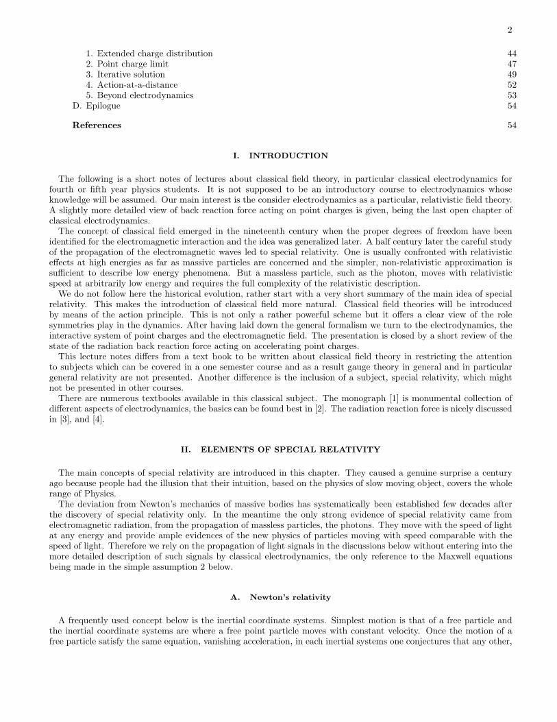
FIG. 2: The arrival of the light to B and C are simultaneous (|AB|′ = |AC|′) in the inertial system (ct, x, y, x) but the lightsignals arrive earlier to B than C in the inertial system (ct′, x′, y′, x′).

The clocks, synchronized in such a manner show immediately one of the most dramatic prediction of specialrelativity, the loss of absolute nature of time. Let us imagine an experimental rearrangement in the coordinate system(x, y, z) of Fig. 2 which contains a light source (A) and two light detectors (B and C), placed at equal distance fromthe source. A light signal, emitted form the source reaches the detectors at the same time in this intertial system. Letus analyze the same process seen from another inertial system (ct′, x′, y′, z′) which is attached to an observer movingwith a constant velocity in the direction of the y axis. A shift by a constant velocity leaves the free particle motionunaccelerated therefore the coordinate system (ct′, x′, y′, z′) where this observes is at rest is inertial, too. But thetime ct′ when the detector C signals the arrival of the light for this moving observer is later than the time ct in theco-moving inertial system. In fact, the light propagates with the same speed in both systems but the detector movesaway form the source int the system (ct′, x′, y′, z′). In a similar manner, the time ct′ when the light reaches detectorB is earlier than ct because this detector moves towards the source. As a result, two events which are in coincidencein one inertial system may correspond to different times in another inertial system. The order of events may changewhen we see them in different inertial systems where the physical laws are supposed to be identical.

C. Invariant length

The finding of the transformation rule for space-time vectors xµ = (ct,x) is rendered simpler by the introductionof some kind of length between events which is the same when seen form different inertial systems. Since the speedof light is the same in every inertial system it is natural to use light in the construction of this length. We definethe distance between two events in such a manner that is is vanishing when there is a light signal which connects thetwo events. The distance square is supposed to be quadratic in the difference of the space-time coordinates, thus theexpression

s2 = c2(t2 − t1)2 − (x2 − x1)

2. (3)

is a natural choice. If s2 is vanishing in one reference frame then the two events can be connected by a light signal.This property is valid in any reference frame, therefore the value s2 = 0 remains invariant during change of inertialsystems.Now we show that s2 6= 0 remains invariant, as well. The change of inertial system may consist of trivial translations

in space-time and spatial rotation which leave the the expression (3) unchanged in an obvious manner. What is leftto show is that a relativistic boost of the inertial system when it moves with a constant speed leaves s2 6= 0 invariant.The so far unspecified transformation of the space-time coordinates between two intertial systems related by a

relativistic boost of velocity v is supposed to generate a transformation s2 → s′2 = F (s2,u) during the boost. We

5

x

t

space−likeseparation

future light−cone

past light−cone

absolut past

separationtime−like

absolut future

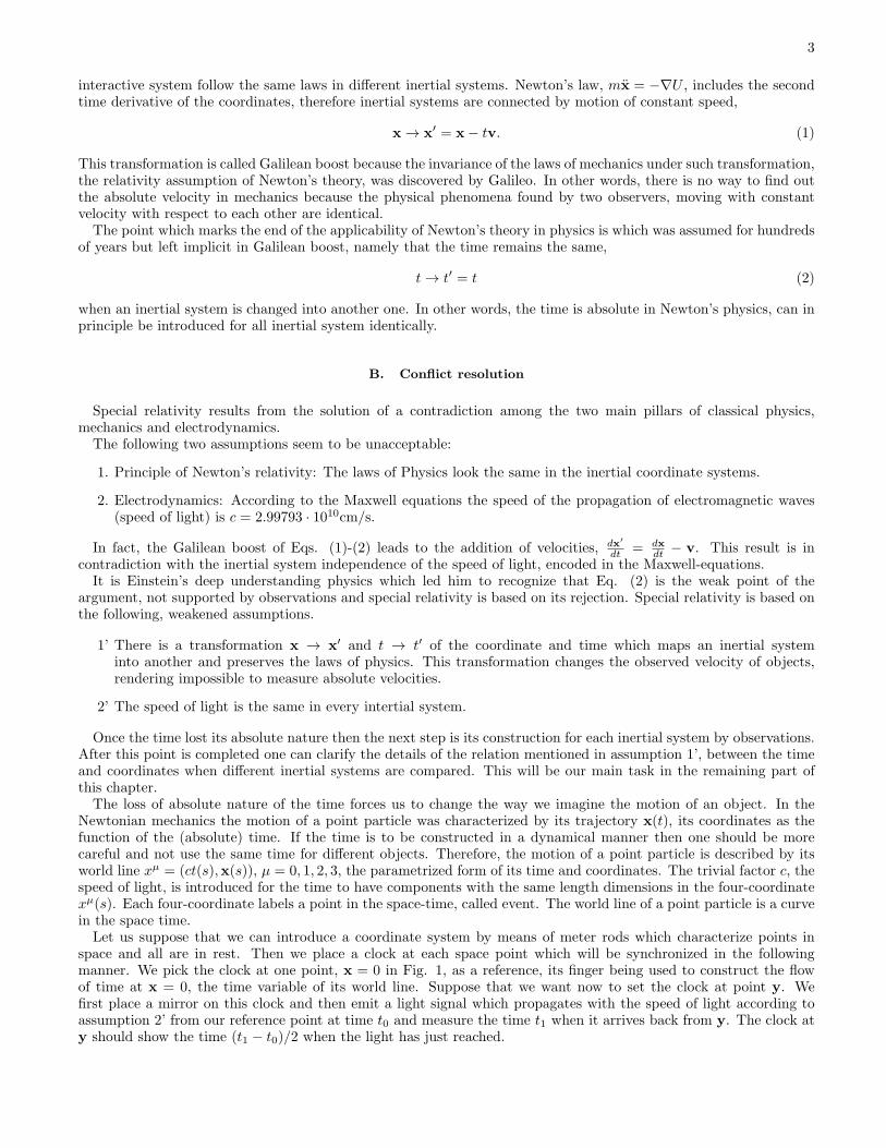
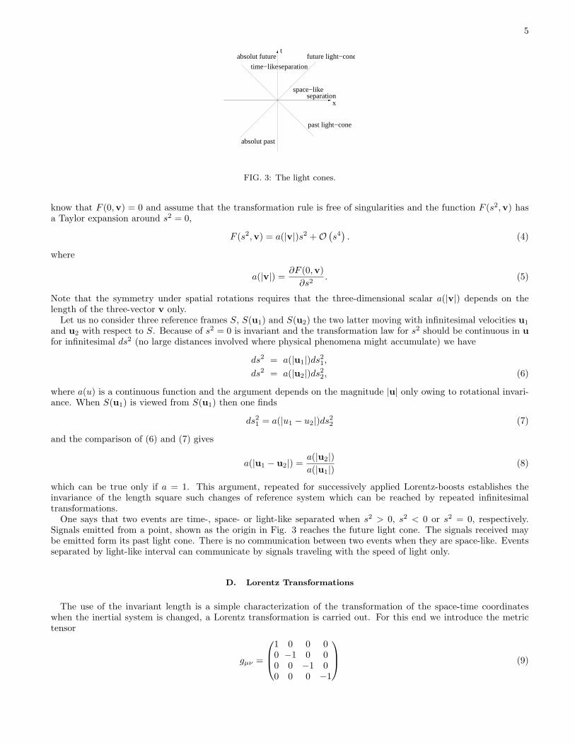
FIG. 3: The light cones.

know that F (0,v) = 0 and assume that the transformation rule is free of singularities and the function F (s2,v) hasa Taylor expansion around s2 = 0,

F (s2,v) = a(|v|)s2 +O(s4). (4)

where

a(|v|) = ∂F (0,v)

∂s2. (5)

Note that the symmetry under spatial rotations requires that the three-dimensional scalar a(|v|) depends on thelength of the three-vector v only.

Let us no consider three reference frames S, S(u1) and S(u2) the two latter moving with infinitesimal velocities u1

and u2 with respect to S. Because of s2 = 0 is invariant and the transformation law for s2 should be continuous in u

for infinitesimal ds2 (no large distances involved where physical phenomena might accumulate) we have

ds2 = a(|u1|)ds21,ds2 = a(|u2|)ds22, (6)

where a(u) is a continuous function and the argument depends on the magnitude |u| only owing to rotational invari-ance. When S(u1) is viewed from S(u1) then one finds

ds21 = a(|u1 − u2|)ds22 (7)

and the comparison of (6) and (7) gives

a(|u1 − u2|) =a(|u2|)a(|u1|)

(8)

which can be true only if a = 1. This argument, repeated for successively applied Lorentz-boosts establishes theinvariance of the length square such changes of reference system which can be reached by repeated infinitesimaltransformations.One says that two events are time-, space- or light-like separated when s2 > 0, s2 < 0 or s2 = 0, respectively.

Signals emitted from a point, shown as the origin in Fig. 3 reaches the future light cone. The signals received maybe emitted form its past light cone. There is no communication between two events when they are space-like. Eventsseparated by light-like interval can communicate by signals traveling with the speed of light only.

D. Lorentz Transformations

The use of the invariant length is a simple characterization of the transformation of the space-time coordinateswhen the inertial system is changed, a Lorentz transformation is carried out. For this end we introduce the metrictensor

gµν =

1 0 0 00 −1 0 00 0 −1 00 0 0 −1

(9)

6

x’

t t’

x

E

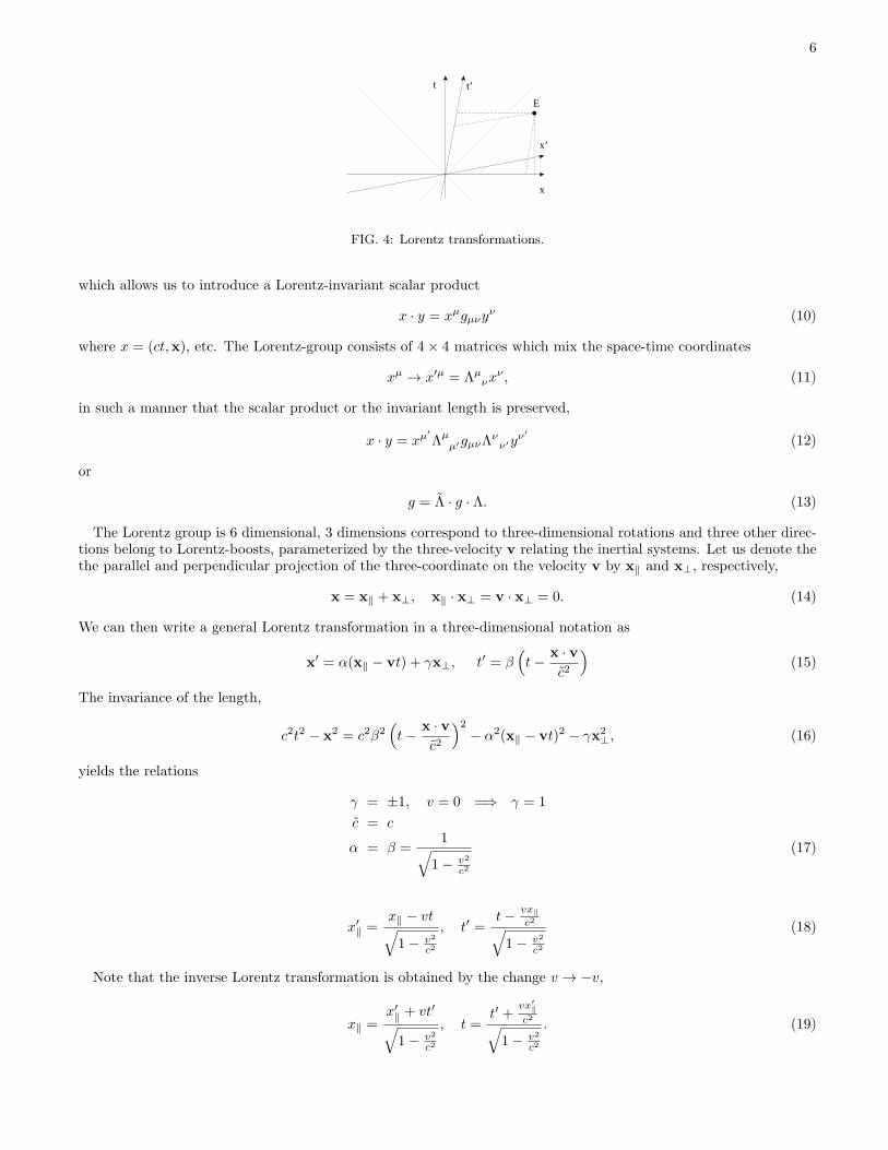
FIG. 4: Lorentz transformations.

which allows us to introduce a Lorentz-invariant scalar product

x · y = xµgµνyν (10)

where x = (ct,x), etc. The Lorentz-group consists of 4× 4 matrices which mix the space-time coordinates

xµ → x′µ = Λµνx

ν , (11)

in such a manner that the scalar product or the invariant length is preserved,

x · y = xµ′

Λµµ′gµνΛ

νν′yν

′

(12)

or

g = Λ · g · Λ. (13)

The Lorentz group is 6 dimensional, 3 dimensions correspond to three-dimensional rotations and three other direc-tions belong to Lorentz-boosts, parameterized by the three-velocity v relating the inertial systems. Let us denote thethe parallel and perpendicular projection of the three-coordinate on the velocity v by x‖ and x⊥, respectively,

x = x‖ + x⊥, x‖ · x⊥ = v · x⊥ = 0. (14)

We can then write a general Lorentz transformation in a three-dimensional notation as

x′ = α(x‖ − vt) + γx⊥, t′ = β(

t− x · vc2

)

(15)

The invariance of the length,

c2t2 − x2 = c2β2(

t− x · vc2

)2

− α2(x‖ − vt)2 − γx2⊥, (16)

yields the relations

γ = ±1, v = 0 =⇒ γ = 1

c = c

α = β =1

√

1− v2

c2

(17)

x′‖ =

x‖ − vt√

1− v2

c2

, t′ =t− vx‖

c2√

1− v2

c2

(18)

Note that the inverse Lorentz transformation is obtained by the change v → −v,

x‖ =x′‖ + vt′√

1− v2

c2

, t =t′ +

vx′‖

c2√

1− v2

c2

. (19)

7

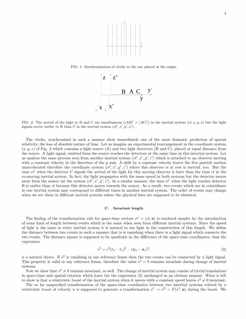
Fig. 4 shows that change of the space-time coordinates during a Lorentz boost. For an Euclidean rotation in twodimensions both axes are rotated by the same angle, here this possibility is excluded by the invariance of the lightcone. As a results the axes are moved by keeping the light cone, shown with dashed lines, unchanged.We remark that there are four disconnected components of the Lorentz group. First note that the determinant

of Eq. (13), det g = det g(det Λ)2 indicates that detΛ = ±1 and there are no infinitesimal Lorentz transformations11 + δΛ such that detΛ(11 + δΛ) 6= detΛ. Thus the spatial inversion split the Lorentz group into two disconnected

sets. Furthermore, observe that the component (00) of Eq. (13), 1 = g00 = (Λ00)

2−∑j(Λj0)

2 implies that Λ00| > 1,

and that time inversion, a Lorentz transformation, splits the :Lorentz group into two disconnected sets. The fourdisconnected components consists of matrices satisfying Eq. (13) and

1. detΛ = 1, Λ00 ≥ 1 (the proper Lorentz group, L↑

+),

2. det Λ = 1, Λ00 ≤ 1,

3. det Λ = −1, Λ00 ≥ 1,

4. det Λ = −1, Λ00 ≤ 1.

Note that one recovers the Galilean boost, x′ = x−vt, in the non-relativistic limit. The argument for the invariance of

the length s2, presented in Chapter II C applies for L↑+ only. But inversions preserve s2 in a obvious manner therefore,

the invariance holds for the whole Lorentz group.One usually needs the full space-time symmetry group, called Poincar group. It is ten dimensional and is the direct

product of the six dimensional Lorentz group and the four dimensional translation group in the space-time.

E. Time dilatation

The proper time τ is the lapse the time measured the coordinate system attached to the system. To find it for anobject moving with a velocity v to be considered constant during a short motion, in a reference system let us expressthe invariant length between two consecutive events,

ref. system of the particle c2dτ2 = c2dt2 − dt2v2 lab. system (20)

which gives

dτ = dt

√

1− v2

c2. (21)

Remarks:

1. A moving clock seems to be slower than a standing one.

2. The time measured by a clock,

1

c

∫ xf

xi

ds (22)

is maximal if the clock moves with constant velocity, ie. its world-line is straight. (Clock following a motion withthe same initial and final point but non-constant velocity seems to be slower than the one in uniform motion.)

F. Contraction of length

The proper length of a rod, ℓ0 = x′2− x′

1, is defined in the inertial system S′ in which the rod is at rest. In anotherinertial system the end points correspond to the world lines

xj =x′j + vt′j√

1− v2

c2

, tj =t′j +

vx′j

c2√

1− v2

c2

. (23)

8

x

x’

t’

t’1

2

E

t t’

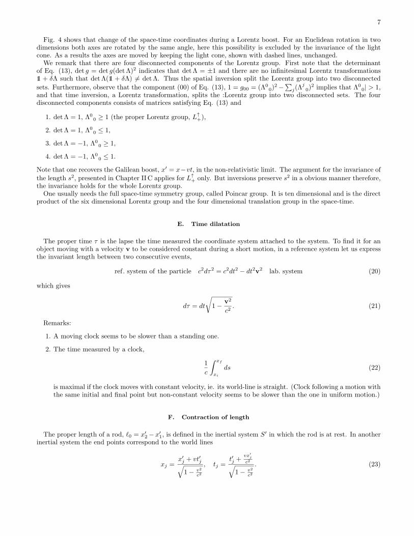
FIG. 5: Lorentz contraction.

The length is read off at equal time, t1 = t2, thus

t′2 − t′1 = − v

c2(x′

2 − x′1) = −

vℓ0c2

(24)

and the invariant length of the space-time vector pointing to the event E is

−ℓ2 = c2(vℓ0c2

)2

− ℓ20, (25)

yielding

ℓ = ℓ0

√

1− v2

c2. (26)

Lorentz contraction is that the length is the longest in the rest frame. It was introduced by Lorentz as an ad hocmechanism to explain the negative result of the Michelson-Moreley experiment to measure the absolute speed of theirlaboratory. It is Einstein’s essential contribution to change this view and instead of postulating a fundamental effecthe derived it by the detailed analysis of the way length are measured in moving inertial system. Thus the contractionof the length has nothing to do with real change in the system, it reflects the specific features of the way observationsare done only.

G. Transformation of the velocity

As mentioned above, the Galilean boost (1)-(2) leads immediately to the addition of velocities, dxdt → dx

dt − v. Thisrule is in contradiction with the invariance of the speed of light under Lorentz boosts. It was mentioned that theresolution of this conflict is the renounce of the absolute nature of the time. This must introduce non-linear pieces inthe transformation law of the velocities. To find them we denote by V the velocity between the inertial systems Sand S′,

dx‖ =dx′

‖ + V dt′√

1− V 2

c2

, dx⊥ = dx′⊥, dt =

dt′ +V dx′

‖

c2√

1− V 2

c2

. (27)

Then

dt

dt′=

1 +V v′

‖

c2√

1− V 2

c2

(28)

and the velocity transform as

v‖ =v′‖ + V

1 +V v′

‖

c2

, v⊥ = v′⊥

√

1− V 2

c2

1 +V v′

‖

c2

. (29)

Note that

9

1. the rule of addition of velocity is valid for v/c≪ 1,

2. if v = c then v′ = c,

3. the expressions are not symmetrical for the exchange of v and V

H. Four-vectors

The space-time coordinates represent the contravariant vectors xµ = (ct,x). In order to eliminate the metric tensorfrom covariant expressions we introduce covariant vectors whose lower index is obtained by multiplying with the metrictensor, xµ = gµνx

ν . Thus allows us to leave out the metric tensor from the scalar product, x · y = xµgµνyν = xµyµ.

The inverse of the metric tensor gµν is denoted by gµν , gµρgρν = δµν .Identities for Lorentz transformations:

g = Λ · g · ΛΛ−1 = g−1 · Λ · g = (g · Λ · g−1)tr

x′µ = (Λ · x)µ = Λµνx

ν

xµ = (g · Λ · g−1) µν x′ν = x′νΛ µ

ν = (x′ · Λ)µx′µ = (g · Λ · x)µ = (g · Λ · g−1 · g · x)µ = Λ ν

µ xν

xµ = x′νΛ

νµ = (x′ · Λ)µ (30)

One can define contravariant tensors which transform as

Tµ1···µn = Λµ1ν1· · ·Λµn

νnT ν1···νn , (31)

covariant tensors with the transformation rule

Tµ1···µn= Λν1

µ1· · ·Λνn

µnTν1···νn

(32)

and mixed tensors which satisfy

T ρ1···ρmµ1···µn

= Λρ1κ1· · ·Λρm

κmΛν1

µ1· · ·Λνn

µnTκ1···κmν1···νn

. (33)

There are important invariant tensors, for instance the metric tensor is preserved, gµν′ = Λµ′

µgµ′ν′Λν′

ν togetherwith its other forms like gµν , g

µν and gνµ. Another important invariant tensor is the completely antisymmetric one

ǫµνρσ where the convention is ǫ0123 = 1. In fact, ǫµνρσ′

= ǫµνρσ detΛ which shows that ǫµνρσ is a pseudo tensor, isremains invariant under proper Lorentz transformation and changes sign during inversions. Note the minus sign inthe relation ǫµνρσ = −ǫµνρσ.

I. Relativistic mechanics

Let us first find the heuristic generalization of Newton’s law for relativistic velocities by imposing Lorentz invariance.The time-like four-velocity of a massive particle is given in terms of its world line xµ(s) as

x =dxµ

ds= x0

(

1,v

c

)

=1

√

1− v2

c2

(

1,v

c

)

, (34)

and it is a unit vector, x2 = 1. The four-acceleration xµ is orthogonal to the four-velocity since

0 =dx2

ds= 2x · x. (35)

The four-momentum, defined by

pµ = mcxµ = (p0,p) =1

√

1− v2

c2

(mc,mv), (36)

10

satisfies the relation p2 = m2c2. The rate of change of the four-momentum defines the four-force,

Kµ = pµ = mcxµ. (37)

The three-vector

F =ds

dtK (38)

can be considered as the relativistic generalization of the force in Newton’s equation,

F = mcd

dt(tv)

=ma

√

1− v2

c2

−d2sdt2

(dsdt )2mcv

=ma

√

1− v2

c2

−ddt

√c2 − v2

c2 − v2mcv

=m

√

1− v2

c2

[

a+v(v · a)

c2(1− v2

c2 )

]

. (39)

The temporal component of Eq. (37),

d

ds(mcx0) =

d

ds

mc√

1− v2

c2

= K0 (40)

leads to the conservation law for the energy. This is because the constraint 0 = mcx · x = K · x gives

K0x0 = Ku = t2Fv. (41)

This condition, written as

d

dtE(v) = Fv (42)

leads to the expression

E(v) =mc2

√

1− v2

c2

(43)

of the kinetic energy. We have therefore

pµ =

(E

c,p

)

, (44)

and the relation p2 = m2c2 leads to the dispersion relation

E2

c2= p2 +m2c2. (45)

Note that the unusual relativistic correction in the three-force (38) is non-vanishing when the velocity is not perpen-dicular to the acceleration, i.e. the kinetic energy is not conserved and work done by the force on the particle.

J. Lessons of special relativity

Special relativity grew out from the unsuccessful experimental attempts of measuring absolute velocities. Thisnegative results is incorporated into the dynamics by postulating a symmetry of the fundamental laws in agreement

11

with Maxwell equations. The most radical consequences of this symmetry concerns the time. It becomes non-absolute, has to be determined dynamically for each system instead of assumed to be available before any observation.Furthermore, two events which coincide in one reference frame may appear in different order in time in other referenceframes, the order of events in time is not absolute either. The impossibility of measuring absolute accelerationand further, higher derivatives of the coordinates with respect to the time is extended in general relativity to thenonavailability of the coordinate system before measurements where the space-time coordinates are constructed bythe observers.The dynamical origin of time motivates the change of the trajectory x(t) as a fundamental object of non-relativistic

mechanics to world line xµ(s) where the reference system time x0 is parametrized by the proper time or simply aparameter of the motion s. The world line offers a surprising extension of the non-relativistic motion by letting x0(s)non-monotonous function. Turning point where time turns back along the world line is interpreted in the quantumcase as an events where a particle-anti particle pair is created or annihilated.We close this short overview of special relativity with a warning. The basic issues of this theory , such as meter

rods and clocks are introduced on the macroscopic level. Though the formal implementation of special relativity isfully confirmed in the quantum regime their interpretation in physical term, e.g. the speed of propagation of lightwithin an atom, is neither trivial nor parallel with the macroscopic reasoning.

III. CLASSICAL FIELD THEORY

A. Why Classical Field Theory?

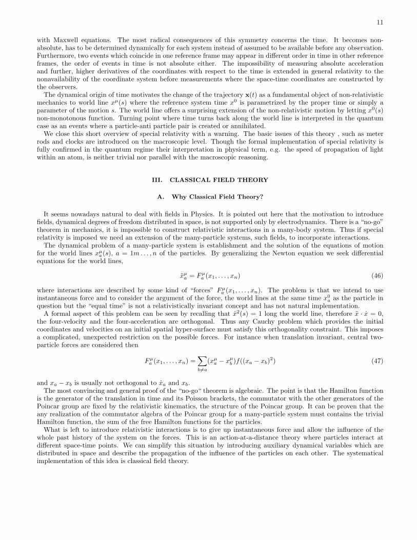
It seems nowadays natural to deal with fields in Physics. It is pointed out here that the motivation to introducefields, dynamical degrees of freedom distributed in space, is not supported only by electrodynamics. There is a “no-go”theorem in mechanics, it is impossible to construct relativistic interactions in a many-body system. Thus if specialrelativity is imposed we need an extension of the many-particle systems, such fields, to incorporate interactions.The dynamical problem of a many-particle system is establishment and the solution of the equations of motion

for the world lines xµa(s), a = 1m. . . , n of the particles. By generalizing the Newton equation we seek differential

equations for the world lines,

xµa = Fµ

a (x1, . . . , xn) (46)

where interactions are described by some kind of “forces” Fµa (x1, . . . , xn). The problem is that we intend to use

instantaneous force and to consider the argument of the force, the world lines at the same time x0a as the particle in

question but the “equal time” is not a relativistically invariant concept and has not natural implementation.A formal aspect of this problem can be seen by recalling that x2(s) = 1 long the world line, therefore x · x = 0,

the four-velocity and the four-acceleration are orthogonal. Thus any Cauchy problem which provides the initialcoordinates and velocities on an initial spatial hyper-surface must satisfy this orthogonality constraint. This imposesa complicated, unexpected restriction on the possible forces. For instance when translation invariant, central two-particle forces are considered then

Fµa (x1, . . . , xn) =

∑

b 6=a

(xµa − xµ

b )f((xa − xb)2) (47)

and xa − xb is usually not orthogonal to xa and xb.The most convincing and general proof of the “no-go“ theorem is algebraic. The point is that the Hamilton function

is the generator of the translation in time and its Poisson brackets, the commutator with the other generators of thePoincar group are fixed by the relativistic kinematics, the structure of the Poincar group. It can be proven that theany realization of the commutator algebra of the Poincar group for a many-particle system must contains the trivialHamilton function, the sum of the free Hamilton functions for the particles.

What is left to introduce relativistic interactions is to give up instantaneous force and allow the influence of thewhole past history of the system on the forces. This is an action-at-a-distance theory where particles interact atdifferent space-time points. We can simplify this situation by introducing auxiliary dynamical variables which aredistributed in space and describe the propagation of the influence of the particles on each other. The systematicalimplementation of this idea is classical field theory.

12

B. Variational principle

Our goal in Section is to obtain equations of motion which are local in space-time and are compatible with certainsymmetries in a systematic manner. The basic principle is to construct equations which remain invariant undernonlinear transformations of the coordinates and the time. It is rather obvious that such a gigantic symmetry rendersthe resulting equations much more useful.Field theory is a dynamical system containing degrees of freedom, denoted by φ(x), at each space point x. The

coordinate φ(x) can be a single real number (real scalar field) or consist n-components (n-component field). Ourgoal is to provide an equation satisfied by the trajectory φcl(t,x). The index cl is supposed to remind us that thistrajectory is the solution of a classical (as opposed to a quantum) equation of motion.This problem will be simplified in two steps. First we restrict x to a single value, x = x0. The n-component field

φ(x0) can be thought as the coordinate of a single point particle moving in n-dimensions. We need the equationsatisfied by the trajectory of this particle. The second step of simplification is to reduce the n-dimensional functionφ(x0) to a single point on the real axis.

1. Single point on the real axis

We start with a baby version of the dynamical problem, the identification of a point on the real axis, xcl ∈ R, in amanner which is independent of the re-parametrization of the real axis.The solution is that the point is identified by specifying a function with vanishing derivative at xcl only:

df(x)

dx |x=xcl

= 0 (48)

To check the re-parametrization invariance of this equation we introduce new coordinate y by the function x = x(y)and find

df(x(y))

dy |y=ycl

=df(x)

dx |x=xcl︸ ︷︷ ︸

0

dx(y)

dy |y=ycl

= 0 (49)

We can now announce the variational principle. There is simple way of rewriting Eq. (48) by performing aninfinitesimal variation of the coordinate x→ x+ δx, and writing

f(xcl + δx) = f(xcl) + δf(xcl)

= f(xcl) + δx f ′(xcl)︸ ︷︷ ︸

0

+δx2

2f ′′(xcl) +O

(δx3). (50)

The variation principle, equivalent of Eq. (48) is

δf(xcl) = O(δx2), (51)

stating that xcl is characterized by the property that an infinitesimal variation around it, xcl → xcl + δx, induces anO(δx2)change in the value of f(xcl).

2. Non-relativistic point particle

We want to identify a trajectory of a non-relativistic particle in a coordinate choice independent manner.Let us identify a trajectory xcl(t) by specifying the coordinate at the initial and final time, xcl(ti) = xi, xcl(tf ) = xf

(by assuming that the equation of motion is of second order in time derivatives) and consider a variation of thetrajectory x(t): x(t) → x(t) + δx(t) which leaves the initial and final conditions invariant (ie. does not modify thesolution). Our function f(x) of the previous section becomes a functional, called action

S[x(·)] =∫ tf

ti

dtL(x(t), x(t)) (52)

13

involving the Lagrangian L(x(t), x(t)). (The symbol x(·) in the argument of the action functional is supposed toremind us that the variable of the functional is a function. It is better to put a dot in the place of the independentvariable of the function x(t) otherwise the notation S[x(t)] can be mistaken with an embedded function S(x(t)).) Thevariation of the action is

δS[x(·)] =

∫ tf

ti

dtL

(

x(t) + δx(t), x(t) +d

dtδx(t)

)

−∫ tf

ti

dtL(x(t), x(t))

=

∫ tf

ti

dt

[

L(x(t), x(t)) + δx(t)δL(x(t), x(t))

δx

+d

dtδx(t)

δL(x(t), x(t))

δx+O

(δx(t)2

)−∫ tf

ti

dtL(x(t), x(t))

]

=

∫ tf

ti

dtδx(t)

[δL(x(t), x(t))

δx− d

dt

δL(x(t), x(t))

δx

]

+ δx(t)︸ ︷︷ ︸

0

δL(x(t), x(t))

δx

∣∣∣∣

ti

tf

+O(δx(t)2

)(53)

The variational principle amounts to the suppression of the integral in the last line for an arbitrary variation, yieldingthe Euler-Lagrange equation:

δL(x, x)

δx− d

dt

δL(x, x)

δx= 0 (54)

The generalization of the previous steps for a n-dimensional particle gives

δL(x, x)

δx− d

dt

δL(x, x)

δx= 0. (55)

It is easy to check that the Lagrangian

L = T − U =m

2x2 − U(x) (56)

leads to the usual Newton equation

mx = −∇U(x). (57)

It is advantageous to introduce the generalized momentum:

p =∂L(x, x)

∂x(58)

which allows to write the Euler-Lagrange equation as

p =∂L(x, x)

∂x(59)

The coordinate not appearing in the Lagrangian in an explicit manner is called cyclic coordinate,

∂L(x, x)

∂xcycl= 0. (60)

For each cyclic coordinate there is a conserved quantity because the generalized momentum of a cyclic coordinate,pcycl is conserved according to Eqs. (58) and (60).

3. Relativistic particle

After the heuristic generalization of the non-relativistic Newton’s law let us consider now more systematically therelativistically invariant variational principle. The Lorentz invariant action must be proportional to the invariantlength of the world-line, this latter being the only invariant of the problem. Dimensional considerations lead to

S = −mc

∫ sf

si

ds =

∫ τf

τi

dτLτ (61)

14

where τ is an arbitrary parameter of the world-line and the corresponding Lagrangian is

Lτ = −mc√

x′µgµνx′ν , (62)

where f ′(τ) = df(τ)dτ . The Lagrangian

L = −mc2√

1− v2

c2= −mc2 +

v2

2m+O

(v4

c2

)

(63)

corresponds to the integrand when τ is the time and justifies the dimensionless constant in the definition of the action(61).We have immediately the energy-momentum

p =∂L

∂v=

mv√

1− v2

c2

E = pv − L =mc2

√

1− v2

c

= mc2 +v2

2m+O

(v4

c2

)

. (64)

The variation of the world-line,

δS =

∫ xf

xi

dτ

(δLτ

δxµδxµ +

∂Lτ

∂x′µδx′µ

)

=∂Lτ

∂x′µδxµ

∣∣∣∣

xf

xi

+

∫ xf

xi

dτδxµ

(∂Lτ

∂xµ− d

dτ

∂Lτ

∂x′µ

)

, (65)

leads to the Euler-Lagrange equation

0 = mcd

dτ

x′µ

√x′2

= mcx′′µx′2 − x′µx′ · x′′

(x′2)3/2

=mc√x′2

Tµνx′′ν , (66)

where the projector into the transverse directions to the four-velocity,

Tµν = gµν − x′µx′ν

x′2(67)

takes care that the infinitesimal change of the time-like unit vector x′µ/√x′2, as given in the first equation of (66)

is orthogonal to the itself. It is obviously the simplest to use teh invariant length s as parameter which makes thefour-acceleration automativally orthogonal to the four-velocity and the equation of motion reads as

0 = mcxµ. (68)

Note that if one uses the invariant length in the place of the the parameter τ from the very beginning in the actionthen the variations are constrained by the condition x · δx = 0. To allow arbitrary variations one needs either a freeparametrisation of the world line or a Lagrange multiplyer to handle the constraint x2 = 1 in the action. Note thatthe momentum, defined as

pµ = − δS

δxµf

, (69)

is independent of the choice of parametrisation and given by pµ = mcxν .The projection of the non-relativistic angular momentum on a given unit vector n can be defined by the derivative

of the action with respect to the angle of rotation around n. Such a rotation generates δx = δRx = δφn×x and gives

δS

δφ=

δS

δxℓf

δxℓ

δφ= pRx = p(n× x) = n(x× p). (70)

15

The relativistic generalization of this procedure is δxµ = δLµνxν ,

δS

δφ=

δS

δxρ

δxρ

δφ= −pµLµνx

ν =1

2Lµν(p

νxµ − pµxν) (71)

yielding

Mµν = xµpν − pµxν . (72)

4. Scalar field

We turn now the dynamical variables which were evoked in avoiding the “no-go“ theorem, fields. We assume thesimple case where there are n scalar degree of freedom at each space point, a scalar field φa(x), a = 1, . . . , n whosetime dependence gives a space-time dependent field φa(x).To establish the variational principle we consider the variation of the trajectory φ(x)

φ(x)→ φ(x) + δφ(x), δφ(ti,x) = δφ(tf ,x) = 0. (73)

The variation of the action

S[φ(·)] =∫

V

dtd3x︸ ︷︷ ︸

dx

L(φ, ∂φ) (74)

is

δS =

∫

V

dx

(∂L(φ, ∂φ)

∂φaδφa +

∂L(φ, ∂φ)

∂∂µφaδ∂µφa

)

+O(δ2φ)

=

∫

V

dx

(∂L(φ, ∂φ)

∂φaδφa +

∂L(φ, ∂φ)

∂∂µφa∂µδφa

)

+O(δ2φ)

=

∫

∂V

dsµδφa∂L(φ, ∂φ)

∂∂µφa

+

∫

V

dxδφa

(∂L(φ, ∂φ)

∂φa− ∂µ

∂L(φ, ∂φ)

∂∂µφa

)

+O(δ2φ)

(75)

The first term for µ = 0,

∫

∂V

ds0δφa∂L(φ, ∂φ)

∂∂0φa=

∫

t=tf

d3x δφa︸︷︷︸

0

∂L(φ, ∂φ)

∂∂0φa

−∫

t=ti

d3x δφa︸︷︷︸

0

∂L(φ, ∂φ)

∂∂0φa= 0 (76)

is vanishing because there is no variation at the initial and final time. When µ = j then

∫

∂V

dsjδφa∂L(φ, ∂φ)

∂∂jφa=

∫

xj=∞

dsjδφa∂L(φ, ∂φ)

∂∂jφa︸ ︷︷ ︸

0

−∫

xj=−∞

dsjδφa∂L(φ, ∂φ)

∂∂jφa︸ ︷︷ ︸

0

= 0 (77)

and it is still vanishing because we are interested in the dynamics of localized systems and the interactions are supposedto be short ranged. Therefore, φ = 0 at the spatial infinities and the Lagrangian is vanishing. The suppression of thesecond term gives the Euler-Lagrange equation

∂L(φ, ∂φ)

∂φa− ∂µ

∂L(φ, ∂φ)

∂∂µφa= 0. (78)

16

Let us consider a scalar field as an example. The four momentum is represented by the vector operator pµ =

−(

~

ic∂0,~

i~∂)

in Quantum Mechanics which leads to the Lorentz invariant invariant Klein-Gordon equation

0 = (p2 −m2c2)φa = −~2(

∂µ∂µ +

m2c2

~2

)

φa, (79)

generated by the Lagrangian

L =1

2(∂φ)2 − m2c2

2~2φ2 =⇒ 1

2(∂φ)2 − m2

2φ2. (80)

The parameter m can be interpreted as mass because the plane wave solution

φk(x) = e−ik·x (81)

to the equation of motion satisfies the mass shell condition,

~2k2 = m2c2 (82)

c.f. Eq. (45).One may introduce a relativistically invariant self-interaction by means of a potential V (φ),

L =1

2(∂φ)2 − m2

2φ2 − V (φ) (83)

and the corresponding equation of motion is

(∂µ∂µ +m2) = −V ′(φ). (84)

C. Noether theorem

It is shown below that there is a conserved current for each continuous symmetry.Symmetry: A transformation of the space-time coordinates xµ → x′µ, and the field φa(x)→ φ′

a(x) preserves theequation of motion. Since the equation of motion is obtained by varying the action, the action should be preservedby the symmetry transformations. A slight generalization is that the action can in fact be changed by a surface termwhich does not influence its variation, the equation of motion at finite space-time points. Therefore, the symmetrytransformations satisfy the condition

L(φ, ∂φ)→ L(φ′, ∂′φ′) + ∂′µΛ

µ (85)

with a certain vector function Λµ(x′).Continuous symmetry: There are infinitesimal symmetry transformations, in an arbitrary small neighborhood

of the identity, xµ → xµ + δxµ, φa(x) → φa(x) + δφa(x). Examples: Rotations, translations in the space-time, andφ(x)→ eiαφ(x) for a complex field.Conserved current: ∂µj

µ = 0, conserved charge: Q(t):

∂0Q(t) = ∂0

∫

V

d3xj0 = −∫

V

d3x∂vj = −∫

∂V

ds · j (86)

It is useful to distinguish external and internal spaces, corresponding to the space-time and the values of the fieldvariable. Eg.

φa(x) : R4

︸︷︷︸

external space

→ Rm

︸︷︷︸

internal space

. (87)

Internal and external symmetry transformations act on the internal or external space, respectively.

17

1. Point particle

The main points of the construction of the Noether current for internal symmetries can be best understood in theframework of a particle. To find the analogy of the internal symmetries let us consider a point particle with thecontinuous symmetry x→ x+ ǫf(x) for infinitesimal ǫ,

L(x, x) = L(x+ ǫf(x), x+ ǫ(x · ∂)f(x)) +O(ǫ2). (88)

Let us introduce a new, time dependent coordinates, y(t) = y(x(t)), based on the solution of the equation of motion,xcl(t), in such a manner that one of them will be y1(t) = ǫ(t), where x(t) = xcl(t) + ǫ(t)f(xcl(t)). There will be n− 1other new coordinates, yℓ, ℓ = 2, . . . , n whose actual form is not interesting for us. The Lagrangian in terms of thenew coordinates is defined by L(y, y) = L(y(x), y(x)). The ǫ-dependent part assumes the form

L(ǫ, ǫ) = L(xcl + ǫf(xcl), xcl + ǫ(xcl · ∂)f(xcl) + ǫf(xcl)) +O(ǫ2). (89)

What is the equation of motion of this Lagrangian? Since the solution is ǫ(t) = 0 it is sufficient to retain the O (ǫ)contributions in the Lagrangian only,

L(ǫ, ǫ)→ L(1)(ǫ, ǫ) = ǫ∂L(xcl, xcl)

∂x· f(xcl)

+∂L(xcl, xcl)

∂x[ǫ(xcl · ∂)f(xcl) + ǫf(xcl)] (90)

up to an ǫ-independent constant. The corresponding Euler-Lagrange equation is

∂L(1)(ǫ, ǫ)

∂ǫ− d

dt

∂L(1)(ǫ, ǫ)

∂ǫ= 0. (91)

(this is the point where the formal invariance of the equation of motion under nonlinear, time dependent transforma-tions of the coordinates is used). According to Eq. (88) ǫ is a cyclic coordinate,

∂L(ǫ, ǫ)

∂ǫ= 0 (92)

and its generalized momentum,

pǫ =∂L(ǫ, ǫ)

∂ǫ(93)

is conserved.Let us now consider two important examples. The external space transformation of field theory corresponds to the

shift of the time, t → t + ǫ which induces x(t) → x(t − ǫ) = x(t) − ǫx(t) for infinitesimal ǫ. This is a symmetry aslong as the Hamiltonian (and the Lagrangian) does not contain explicitly the time. In fact, the action changes by aboundary contribution only which can be seen by expanding the Lagrangian in time around t− ǫ,

∫ tf

ti

dtL(x(t), x(t)) =

∫ tf

ti

dt

[

L(x(t− ǫ), x(t− ǫ)) + ǫdL(x(t), x(t))

dt

]

(94)

up to O(ǫ2)terms and as a result the variational equation of motion remains unchanged. But the continuation of the

argument is slightly different from the case of internal symmetry. We consider ǫ as a time dependent function whichgenerates a transformation of the coordinate, x(t)→ x(t− ǫ(t)) = x(t)− ǫ(t)x(t) +O

(ǫ2). The Lagrangian of ǫ(t) as

new coordinate for the choice x(t) = xcl(t) is

L(ǫ, ǫ) = L(xcl(t− ǫ), xcl(t− ǫ))− L(xcl(t), xcl(t))

= −ǫxcl∂L(xcl, xcl)

∂x− dǫxcl

dt

∂L(xcl, xcl)

∂x

= −ǫxcl∂L(xcl, xcl)

∂x− ǫxcl

∂L(xcl, xcl)

∂x︸ ︷︷ ︸

−ǫdL(xcl,xcl)

dt

−ǫxcl∂L(xcl, xcl)

∂x

= −ǫ[dL(xcl, xcl)

dt− d

dt

(∂L(xcl, xcl)

∂xxcl

)]

− d

dt

(∂L(xcl, xcl)

∂xclǫxcl

)

(95)

18

up to an ǫ-independent constant andO(ǫ2)contributions and its equation of motion, Eq. (91), assures the conservation

of the energy,

H =∂L(x, x)

∂xx− L(x, x). (96)

As another application of Noether theorem we consider now a particle moving in a spherically symmetric potential.The Lagrangian

L(x, x) =m

2x2 − U(|x|) (97)

displaying rotational symmetry. Infinitesimal rotation around the axis defined by the unit vector n by angle ǫ canbe written as δx = ǫn × x + O

(ǫ2). We use a time-dependent rotation, described by a function ǫ(t) satisfying the

constraint ǫ(ti) = ǫ(tf ) = 0 to parameterize a variation x(t) → x(t) + ǫ(t)n × x(t) around a solution x(t) of theEuler-Lagrange equations. We find now the Euler-Lagrange equation for ǫ(t) which, we know ahead is satisfied byǫ(t) = 0. The Lagrangian in terms of ǫ(t) is

L(ǫ, ǫ) =m

2(x+ ǫn× x)2 − U(|x+ ǫn× x|) +O

(ǫ2)

= L(x, x) +mǫx(n× x) +O(ǫ2). (98)

The infinitesimal rotation angle ǫ is cyclic parameter of the O (ǫ) Lagrangian due to the rotational invariance of theproblem. Hence the Euler-Lagrange equation for ǫ is

d

dtnL = 0 (99)

where L = x×mx and the identity x(n× x) = n(x× x) has been used.

2. Internal symmetries

An internal symmetry transformation of field theory acts on the internal space only. We shall consider linearlyrealized internal symmetries for simplicity where

δxµ = 0, δiφa(x) = ǫ τab︸︷︷︸

generator

φb(x). (100)

This transformation is a symmetry,

L(φ, ∂φ) = L(φ+ ǫτφ, ∂φ+ ǫτ∂φ) +O(ǫ2). (101)

Let us introduce new ”coordinates”, ie. new field variable, Φ(φ), in such a manner that Φ1(x) = ǫ(x) where φ(x) =φcl(x) + ǫ(x)τφcl(x), φcl(x) being the solution of the equations of movement. The linearized Lagrangian for ǫ(x) is

L(ǫ, ∂ǫ) = L(φcl + ǫτφ(x), ∂φcl + ∂ǫτφ(x) + ǫτ∂φ(x))

→ ǫτ∂L(φcl, ∂φcl)

∂φ+ [∂ǫτφ(x) + ǫτ∂φ(x)]

∂L(φcl, ∂φcl)

∂∂φ. (102)

The symmetry, Eq. (101), indicates that ǫ is a cyclic coordinate and the equation of motion

∂L(ǫ, ∂ǫ)

∂ǫ− ∂µ

∂L(ǫ, ∂ǫ)

∂∂µǫ= 0. (103)

shows that the current,

Jµ = −∂L(ǫ, ∂ǫ)

∂∂µǫ= −∂L(φ, ∂φ)

∂∂µφτφ (104)

defined up to a multiplicative constant as the generalized momentum of ǫ, is conserved. Notice that (i) we have anindependent conserved current corresponding to each independent direction in the internal symmetry group and (ii)the conserved current is well defined up to a multiplicative constant only.

19

Let us consider a complex scalar field with symmetry φ(x)→ eiαφ(x) as an example. The theory is defined by theLagrangian

L = ∂µφ∗∂µφ−m2φ∗φ− V (φ∗φ) (105)

where it is useful to considered φ and φ∗ as independent variables. The infinitesimal transformations δφ = iǫφ,δφ∗ = −iǫφ∗ yield the conserved current

jµ =i

2(φ∗∂µφ− ∂µφ∗φ) (106)

up to a multiplicative constant.

3. External symmetries

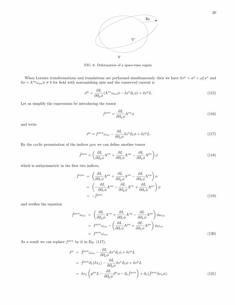
The most general transformations leaving the action invariant may act in the external space, too. Let us considerthe translations, xµ → x′µ = xµ + δxµ and φ(x) → φ′(x′) = φ(x) + δφ(x) where δφ(x) = −δxµ∂µφ(x). We shall useinfinitesimal, space-time dependent δxµ(x), to parametrize a particular variation of the field. The variation of theaction is

δS =

∫

V

dxδL+

∫

V ′−V

dxL

=

∫

V

dxδL+

∫

∂V

dSµδxµL (107)

according to Fig. 6 what can be written as

δS =

∫

V

dx

(∂L

∂φ− ∂µ

∂L

∂∂µφ

)

δφ+

∫

∂V

dSµ

(∂L

∂∂µφδφ+ δxµL

)

. (108)

due to the relation ∂µδφ(x) = ∂µ[φ(x− δxµ(x))− φ(x)] = δ∂µφ(x). For field configurations satisfying the equation ofmotion the first integral is vanishing and we find

δS =

∫

∂V

dSµδxν

(

Lgµν −∂L

∂∂µφ∂νφ

)

(109)

leaving the current, defined for translations, ie. space-time independent δxµ(x) = ǫµ

Jµ = ǫν(

Lgµν −∂L

∂∂µφ∂νφ

)

(110)

conserved. Hence the canonical energy-momentum tensor, containing the four conserved current,

Tµνc =

∂L

∂∂µφ∂νφ− Lgµν (111)

obeys the conservation law

∂µTµνc = 0. (112)

Therefore,

P ν =

∫

d3xT 0νc (113)

can be identified by the energy-momentum vector and we have the form

Tµνc =

(ǫ cp1cS σ

)

(114)

where ǫ denotes the energy density, p stands for the momentum density, S is the energy flux and σjk is the flux of pk

in the direction j.

20

xδ

V

V’

FIG. 6: Deformation of a space-time region.

When Lorentz transformations and translations are performed simultaneously then we have δxµ = aµ + ωµν x

ν andδφ = Λνµωµνφ 6= 0 for field with nonvanishing spin and the conserved current is

Jµ =∂L

∂∂µφ(Λνκωκνφ− δxν∂νφ) + δxµL. (115)

Let us simplify the expressions be introducing the tensor

fµνκ =∂L

∂∂µφΛνκφ (116)

and write

Jµ = fµνκωκν −∂L

∂∂µφδxν∂νφ+ δxµL. (117)

By the cyclic permutation of the indices µνκ we can define another tensor

fµνκ =

(∂L

∂∂µφΛνκ +

∂L

∂∂νφΛκµ − ∂L

∂∂κφΛµν

)

φ (118)

which is antisymmetric in the first two indices,

fνµκ =

(∂L

∂∂νφΛµκ +

∂L

∂∂µφΛκν − ∂L

∂∂κφΛνµ

)

φ

=

(

− ∂L

∂∂νφΛκµ − ∂L

∂∂µφΛνκ +

∂L

∂∂κφΛµν

)

φ

= −fµνκ (119)

and verifies the equation

fµνκωνκ =

(∂L

∂∂µφΛνκ +

∂L

∂∂νφΛκµ − ∂L

∂∂κφΛµν

)

φωνκ

= fµνκωνκ −(

∂L

∂∂νφΛµκ +

∂L

∂∂κφΛµν

)

φωνκ

= fµνκωνκ. (120)

As a result we can replace fµνκ by it in Eq. (117),

Jµ = fµνκωκν −∂L

∂∂µφδxν∂νφ+ δxµL

= fµνκ∂ν(δxκ)−∂L

∂∂µφδxν∂νφ+ δxµL

= δxκ

(

gµκL− ∂L

∂∂µφ∂κφ− ∂ν f

µνκ

)

+ ∂ν(fµνκδxκφ). (121)

21

The last term J ′µ = ∂ν(fµνκδxκφ) gives a conserved current thus can be dropped and the conserved Noether current

simplifies as

Jµ = Tµν(aν + ωνκxκ) = Tµνaν +

1

2(Tµνxκ − Tµκxν)ωνκ (122)

where we can introduced the symmetric energy momentum tensor

Tµν = Tµνc + ∂κf

µκν (123)

and the tensor

Mµνσ = Tµνxσ − Tµσxν . (124)

Due to∫

∂V

Sµ∂κfµκν =

∫

V

∂µ∂κfµκν = 0 (125)

the energy momentum extracted from Tµν and Tµνc agree and M is conserved

∂µMµνσ = 0, (126)

yielding the relativistic angular momentum

Jνσ =

∫

d3x(T 0νxσ − T 0σxν). (127)

with the usual non-relativistic spatial structure. The energy-momentum tensor Tµν is symmetric because the conser-vation of the relativistic angular momentum, Eq. (126) gives

0 = ∂ρMρµν = ∂ρ(T

ρµxν − T ρνxµ) = T νµ − Tµν . (128)

IV. ELECTRODYNAMICS

The dynamics of the charge-electromagnetic field system will be constructed in two steps, first the motion of thecharges is considered on a prescribed electromagnetic field then the equations of motion are sought for the electromag-netic field in the presence of electric current of charges. Next the energy-momentum content of the electromagneticfield is identified by means of the energy-momentum tensor. Finally, the simplest solution of the equations of motionfor the electromagnetic field in vacuum, the plane waves are considered.

The electromagnetic field dynamics has no non-relativistic limit, the radiation always travels with speed of light.Therefore it is important to keep track of the Lorentz contraction of the charges in order to preserve relativisticinvariance of the full, interacting system. We encounter a serious technical problem when Lorentz contraction, aresult of observations made by light, is imposed on the charges because their world line can not be used anymore asindependent dynamical variable beside the electromagnetic field. To avoid this deadlock one usually goes into thelimit of point charges where the Lorentz contraction is expected to be negligible. But we run into another problemin this limit, classical physics becomes inconsistent close to a point charge due to the strong Coulomb field. Thisproblem, the remnants of Lorentz contraction is reconsidered in the last chapter.

A. Point charge in an external electromagnetic field

The three-dimensional scalar and vector fields make up the four-dimensional vector potential as Aµ = (φ,A) and thesimplest Lorentz invariant Lagrange function we can construct with it is Aµx

µ therefore the action for a point-chargemoving in the presence of a given, external vector potential is

S = −∫ xf

xi

(

mcds+e

cAµdx

µ)

= −∫ xf

xi

(

mcds− e

cA · dx+ eφdt

)

=

∫ τf

τi

Lτdτ, (129)

22

where the index τ in the Lagrangian is a reminder of the variable used to construct the action,

Lτ = −mc√x′2 − e

cAµ(x)x

′µ. (130)

The Euler-Lagrange equation reads

0 =∂Lτ

∂xµ− d

dτ

∂Lτ

∂x′µ

= −e

c∂µAν(x)x

′ν +mcd

dτ

x′µ√x′2

+e

c

d

dτAµ(x)

=mc√x′2

Tµνx′′ν −

e

cFµνx

′ν (131)

where the field-strength is given by

Fµν = ∂µAν(x)− ∂νAµ(x). (132)

It is useful to write this equation for the world line which is parametrized by its invariant length as,

0 = mcxµ −e

cFµν x

ν . (133)

It is advantegous to write the interaction action as a space-time integral involving the current density,

S = −mc

∫

ds− e

c

∫

dxAµ(x)jµ(x). (134)

In the case of a system of charges, xa(t), we have

jµ(x) = c∑

a

∫

dsδ(x− xa(s))xµ

= c∑

a

∫

dsδ(x− xa(s))δ(x0 − x0

a(s))xµ

= c∑

a

δ(x− xa(s))xµ

|x0|

=∑

a

δ(x− xa(s))

︸ ︷︷ ︸

ρ(x)

dxµ

dt. (135)

The relativistically covariant generalization of the non-relativistic current j = ρv for a single charge is indeed

jµ = ρdxµ

dt= (cρ, j) = (cρ, ρv) = ρ

ds

dtxµ (136)

It is easy to verify that the continuity equation

∂µjµ = c∂0ρ+∇ · j

=∑

a

ea[−va(t)∇δ(x− xa(t)) +∇δ(x− xa(t))va(t)] = 0 (137)

is satisfied.

B. Dynamics of the electromagnetic field

The action (136) dos not contain the time derivatives of the vector potential therefore we have to extend ourLagrangian, L→ L+LA, to generate dynamics for the electromagnetic field. The guiding principle is that LA shouldbe

23

1. quadratic in the time derivative of the vector potential to have the usual equation of motion,

2. Lorentz invariant and

3. gauge invariant, ie. remain invariant under the transformation

Aµ → Aµ + ∂µα. (138)

The simplest solution is

LA = − 1

16πFµνFµν (139)

where the factor −1/16π is introduced for later convenience. The complete action is S = Sm + SA where

Sm = −mc∑

a

∫

ds√

xµagµν xν

a (140)

and

SA = −e

c

∑

a

∫

Aµ(x)dxµ − 1

16πc

∫

FµνFµνdx

= −e

c

∑

a

∫

dsdxδ(4)(x− xa(s))Aµ(x)xµ − 1

16πc

∫

FµνFµνdx

=

∫

LAdV dt (141)

with

LA = −e

cjµAµ −

1

16πFµνFµν

= −e

cjµAµ −

1

8π∂µAν∂

µAν +1

8π∂µAν∂

νAµ. (142)

It yields the Maxwell-equations

0 =δL

δAµ− ∂ν

δL

δ∂νAµ= −e

cjµ − 1

4π∂νF

µν . (143)

Note that the necessary condition for the gauge invariance of the action is the current conservation, Eq. (139).A simple calculation shows that any continuously double differentiable vector potential satisfies the Bianchi identity,

∂ρFµν + ∂νFρµ + ∂µFνρ = 0. (144)

The usual three-dimensional notation is achieved by the parametrization Aµ = (φ,A), Aµ = (φ,−A), giving theelectric and the magnetic fields

E = −∂0A−∇φ = −1

c∂tA−∇φ,

H = ∇×A. (145)

Notice that transformation jµ = (cρ, j)→ (cρ,−j) under time reversal and the invariance of the term jµAµ interactionLagrangian requires the transformation law φ→ φ, A→ −A, E→ E, H→ −H for time reversal. The equation

ǫjkℓHℓ = ǫjkℓǫℓmn∇mAn = (δjmδkn − δjnδkm)∇mAn = ∇jAk −∇kAj (146)

relates the electric and magnetic field with the field strength tensor as

Fµν(E,H) =

0 −Ex −Ey −Ez

Ex 0 −Hz Hy

Ey Hz 0 −Hx

Ez −Hy Hx 0

, Fµν(E,H) =

0 Ex Ey Ez

−Ex 0 −Hz Hy

−Ey Hz 0 −Hx

−Ez −Hy Hx 0

(147)

24

One defines the dual field strength as

Fµν =1

2ǫµνρσF

ρσ. (148)

Duality refers to the exchange of the electric and the magnetic fields up to a sign,

F0j = −1

2ǫjkℓF

kℓ = Hj , Fjk = −ǫjkℓF ℓ0 = ǫjkℓEℓ, (149)

giving

Fµν(E,H) = Fµν(H,−E), Fµν(E,H) = Fµν(H,−E). (150)

We have two invariants,

FµνFµν = −2E2 + 2H2

FµνFµν = 4EH (151)

but the first can be used only in classical electrodynamics which is invariant under time reversal. The electromagneticfield is called null-field when both invariants are vanishing, FµνFµν = FµνFµν = 0.The field strength tensor transforms under Lorentz transformations as

φ′ =φ− v

cA‖√

1− v2

c2

, A′‖ =

A‖ − vcφ

√

1− v2

c2

, (152)

and

F⊥⊥′

= F⊥⊥

F ‖⊥′

=F ‖⊥ − v

cF0⊥

√

1− v2

c2

F 0⊥′

=F 0⊥ − v

cF‖⊥

√

1− v2

c2

F ‖0′ = F ‖0 (∼ ǫ01). (153)

For v = (v, 0, 0) we have in the three-dimensional notation

E′‖ = F ‖0′ = E‖, H ′

‖ = F⊥⊥′

= H ′‖,

E′y = F 0⊥′

=Ey − v

cHz√

1− v2

c2

, E′z = F 0⊥′

=Ez +

vcHy

√

1− v2

c2

H ′y = F ‖⊥′

=Hy +

vcEz

√

1− v2

c2

, H ′z = F ‖⊥′

=Hz − v

cEy√

1− v2

c2

, (154)

i.e. the homogeneous electric and magnetic fields transform into each other when seen by an observer moving withconstant speed.The equation of motion (145) can easily be written in three-dimensional notation. The time component is

4πρ = ∇E (155)

and the spatial components

4π

cjk = ∂0F

0k +∇jFjk (156)

yield

4π

cj = −1

c∂tE+∇×H. (157)

The Bianchi identity (146) is non-trivial for µ 6= ν 6= ρ when it gives

0 = ∇H,

0 =1

c∂tH+∇×E. (158)

25

C. Energy-momentum tensor

Let us first construct the energy-momentum tensor for the electromagnetic field by means of the Noether theorem.The translation xν → xν+ǫν is a symmetry of the dynamics therefore we have a conserved current for each space-timedirection ν, (Jµ)ν , which can be rearranged in a tensor, Tµν = (Jµ)ν , given by

Tµνc = −gµνL+

δL

δ∂µAρ∂νAρ = gµν

(1

16πF ρσFρσ +

e

cjρAρ

)

− 1

4πFµρ∂νAρ (159)

for the canonical energy-momentum tensor. The conservation law, ∂µTµνc = 0 suggests the identification of

P ν(t) =

∫

V

d3xT 0νc (t,x) (160)

with the energy-momentum of the system up to a multiplicative constant. But the physical energy-momentum maycontain a freely chosen three index tensor Θµρν as long as Θµρν = −Θρµν because

Tµν → Tµν + ∂ρΘµρν (161)

is still conserved and the charge is changed by a surface term only,

T 0νc → T 0ν

c + ∂jΘ0jν . (162)

This freedom can be used to eliminate an unphysical property of the canonical energy-momentum tensor, namelyits gauge dependence. The choice Θµρν = 1

4πFµρAν gives

Tµν = gµν(

1

16πF ρσFρσ +

e

cjρAρ

)

− 1

4πFµρ∂νAρ +

1

4π∂ρ(F

µρAν)

=gµν

16πF ρσFρσ +

1

4πFµρF ν

ρ + gµνe

cjρAρ +

1

4π∂ρF

µρAν

=gµν

16πF ρσFρσ +

1

4πFµρF ν

ρ + gµνe

cjρAρ − jµAν (163)

where the equation of motion was used in the last equation. The new energy-momentum tensor in the absence of theelectric current, the true energy-momentum tensor of the EM field,

Tµνed =

gµν

16πF ρσFρσ +

1

4πFµρF ν

ρ , (164)

is gauge invariant, symmetric and traceless.The energy-momentum of the EM field is not conserved, there is a continuous exchange of energy-momentum

between the charges and the EM field. The amount of non-conservation, Kν = −∂µTµνed 6= 0, identifies the energy-

momentum density of the charges,

Kν = −∂µ(gµν

16πF ρσFρσ +

1

4πFµρF ν

ρ

)

= − 1

8πF ρσ∂νFρσ −

1

4πFµρ∂µF

νρ − 1

4π∂µF

µρF νρ . (165)

We use the Bianchi identity for the first term and the equation of motion

Kν = − 1

8πF ρσ(−∂ρF ν

σ − ∂σFνρ

︸ ︷︷ ︸

Bianchi

−2∂σF νρ )− 1

cjρF ν

ρ

= − 1

8πF ρσ(∂ρF

νσ + ∂σF

νρ)

︸ ︷︷ ︸

=0

+1

cjρF ν

ρ

= ρF ν0 +

1

cjkF ν

k

= ρF ν0 − 1

cjkF νk. (166)

26

Since

−jkF 0k = jE

ρF ℓ0 = ρEℓ

jkF ℓk = −jkǫℓkmHm (167)

we have the source of the energy-momentum of the EM field

Kµ = (K0,K) =

(1

cjE, ρE+

1

cj×H

)

. (168)

The time-like component is indeed the work done on the charges by the EM field. The spatial components is the rateof change of the momentum of the charges, the Lorentz force.The energy-momentum density of the EM field, P ν = T 0ν , is

P 0 =1

8π(−E2 +H2) +

1

4πE2 =

1

8π(E2 +H2)

P ℓ =1

4πcF 0kF ℓ

k =1

4πcEkǫkℓmHm = − 1

c2Sℓ (169)

where the energy flux-density

S =c

4πE×H (170)

is given by the Poynting vector. In fact, the symmetry of the energy-momentum tensor allows us to identify theenergy flux-density with c times the momentum density.

D. Simple electromagnetic waves in the vacuum

Let us consider first the EM field waves in the absence of charges, the solution of the Maxwell equations, (145) forj = 0. We shall use the Lorentz gauge ∂µA

µ = 0 where the equations of motion are

0 = ∂νFµν = ∂ν∂

µAν −Aµ = −Aµ. (171)

we shall consider plane and spherical waves, solutions which display the same value on parallel planes or concentricspheres.The plane wave solution depends on the combination

tn = t− n · xc

(172)

of the space-time coordinates. The linearity of the Maxwell equation allows us to write the solution as the linearsuperposition

Aµ(x) = A+µ (tn) +A−

µ (t−n) (173)

where(

1

c2∂2t −∆

)

A±µ (x) = A±

µ (t±n) = 0 (174)

for an arbitrary functions A±µ (t), to be determined by the boundary conditions.

The plane wave Aµ(tn) appears in the three-dimensional notation as

H = ∇×A = ∇(

t− n · xc

)

×A′ = −1

cn×A′

E = −1

c∂tA−∇φ = −1

cA′ +

1

cnφ′. (175)

The vectors E, H and n are orthogonal to each others. In fact, the relation

H = −1

cn× (−cE+ nφ′) = n×E (176)

27

shows that H orthogonal both to the direction of the propagation, n and to E. The Lorentz gauge condition,

0 =1

c∂tφ+∇A =

1

cφ′ − 1

cnA′ (177)

together with the second equation in (177) shows that E is orthogonal to n, as well. The orthogonality of E and H

follows from

E ·H =1

c2(A′ − nφ′)n×A′ = 0. (178)

The simple reason of the orthogonality is that we have two vectors, n and A′ at our disposal to generate two othervectors, E and H in a rotationally covariant and gauge invariant manner. The latter requires to use A′ within thevector product n×A′ to find one vector, the other can only be n× (n×A′).

The energy-momentum density

P ν =

(E2 +H2

8π,−E×H

4π

)

=

(E2

4π,−E× (n×E)

4π

)

=E2

4π(1,−n), (179)

is a light-like vector, P 2 = 0.The spherical waves are of the form (175) with

t± = t± r

c(180)

in spherical coordinate system. We consider them in d spatial dimensions where they satisfy the wave equation

∂µ∂µA = 0. We write A±(x) = r

1−d2 a±(t±) where a± is a solution of the equation

0 =

(1

c2∂2t −

1

rd−1∂rr

d−1∂r

)

A±(t±)

=

(1

c2∂2t +

(d− 1)(d− 3)

4r2∂r − ∂2

r

)

a±(t±). (181)

The functions a±(t±) correspond to 1+1 dimensional plane waves in d = 1, 3 only. We consider the latter case wherethe expressions

∇φ(r) = er∂rφ

∇a(r) =1

r2∂r(r

2ar) +cot θ

raθ

∇× a(r) = eφ1

r∂r(raθ)− eθ

1

r∂r(raφ) (182)

for vector operations will be used for φ = u/r, and A = a/r. The magnetic and electric fields are

H = ∇× 1

ra = ∇1

r× a+

1

r∇× a

=1

r2[−er × a− eθ∂r(raφ) + eφ∂r(raθ)]

= ± 1

cr

(eφa

′θ − eθa

′φ

)

= ± 1

crer × a′

E = − 1

rc∂ta−∇

u

r= − 1

rca′ + er

u∓ rcu

′

r2. (183)

Now the relation

H = ∓er ×E (184)

28

shows again that H orthogonal both to the direction of the propagation, er and to E. The Lorentz gauge condition,

0 =1

cru′ +∇1

ra

=1

cru′ +

1

r2

[

−ar +1

r∂r(r

2ar)

]

+cot θ

r2aθ

=1

r2

[r

c(u′ ± a′r) + ar

]

+cot θ

r2aθ (185)

sets aθ = 0. But the electric field is not necesseraly orthogonal to the direction of propagation,

Eer = − 1

rca′r +

u∓ rcu

′

r2= − 1

rca′r +

u

r2+±ar + r

ca′r

r2=

u± arr2

(186)

and the energy-momentum density is not always time-like neither as a result of the compactness of the equal phasesurface.

V. GREEN FUNCTIONS

The Green functions provide a clear and compact solution of linear equations of motion. But the transparency pfthe result hides a drawback, the suppression of the the boundary conditions which are imposed both in space andtime. The spatial boundary conditions are usually simpler, they amount to some suppression of the fields at spatialinfinity when localized phenomena are investigated. The boundary conditions in time are more complicated and aredealt with briefly in the next section.

A. Time arrow problem

The basic equations of Physics, except weak interactions, are invariant under a discrete space-time symmetry, thereversal of the direction of time, T : (t,x) → (−t,x). Despite this symmetry, it is a daily experience that the thissymmetry is not respected in the world around us. It is enough to recall that we are first born and die later, never inthe opposite order. A more tangible example is that the radio transmission arrives at our receivers after its emission,namely the electromagnetic signals travel forward in time rather than backward which is in principle always possiblewith time reversal invariant equations of motion. What eliminates the backward moving electromagnetic waves? Thisis one aspect of the time arrow problem in Physics, the problem of pinning down the direction of time, the dynamicalorigin of the apparent breakdown of the time reversal invariance.This problem can be discussed at four different level. The most obvious is the level of electromagnetic radiation

where it appears as the suppression of backward moving electromagnetic waves in time. It is believed that the originof this problem is not in Electrodynamics and this property of the electromagnetic waves is related to the boundaryconditions chosen in time. We can prescribe the solution we seek in terms of initial or final conditions or even bya mixture of these two possibilities and depending on our choice we see forward or backward going waves or eventheir mixture in the solution. Why are we interested mainly initial problems rather than final condition problems inphysics?A tentative answer comes from Thermodynamics, the non-decreasing nature of entropy in time. It seems that the

composite systems tend to become more complicated and to expand into more irregular regions in the phase spaceas the time elapses. This property is might not be related to the breakdown of the time reversal invariance becauseit must obviously hold for either choice of the time arrow. It seems more to have something to do with the nature ofthe initial conditions we encounter in Physics.The choice of the initial condition leads us to the astrophysical origin of the time arrow. The current cosmological

models, solutions of the formally time reversal invariant Einstein equations of General Relativity, suggest that ourUniverse undergone a singularity in the distant past. This singular initial condition might be the origin of the peculiarfeatures of the choice of the time arrow.Yet another level of this issue is the quantum-classical crossover, the scale regime where quantum effects give rise

to classical physics. Each measurement traverses this crossover, it magnifies some microscopic quantum effects intomacroscopic, classical one. This magnification process, such as the condensation of the drops in the Wilson cloudchamber or the ”click” of a Geiger counter indicating th presence of an energetic particle, breaks the time reversalinvariance. In fact, the end result of the measurements, a classical ”record” created endures the flow of time and cannot be reconverted into microscopic phenomena without macroscopic trace. Hence the deepest level of the breakdown

29

of the time reversal invariance comes from the scale regions because any quantum gravitational problem must behandled by this scheme.Instead of following a more detailed analysis of this dynamical issue we confine the discussion of the separation of

the kinematical aspects of this problem. The question we turn to is the way a certain initial of final condition problemcan be handled within the framework of Classical Field Theory. The problem arises from the use of the variationalprinciple in deriving the equations of motion. The variational equations of motion can not break the time reversalinvariance and can not handle any boundary conditions which does it.We start the discussion with the formal introduction of the Green function. Let us consider a given function of the

time f(t) and the inhomogeneous linear differential equation

Lf = g, (187)

where L is a differential operator acting on the time variable. The Green function satisfies the equation

LtG(t, t′) = δ(t− t′). (188)

The index in Lt is a reminder that the differential operator acts on the variable t of the two variable function G(t, t′).Note that for translation invariant L we have G(t, t′) = G(t − t′). The Dirac-delta is the identify operator on thefunction space, thus G = L−1. The solution of Eq. (189) can now formally be written as

f(t) =

∫

dt′G(t, t′)g(t′). (189)

The time reversal invariance of the equation of motion renders the matrix L(t, t′), representing the operator L inEq. (189) symmetric, L(t, t′) = L(t′, t). Eq. (190) might be interpreted by saying that the Green function is theinverse of the operator L. The inverse of a symmetric matrix is symmetric, as well, G(t, t′) = G(t′, t). But this isin contradiction with our experience that the effect of an external perturbation, represented by the source g appearsafter the perturbation and not before. When the propagation of a signal violates time reversal invariance then theGreen function must contain antisymmetric part. How can this happen?

Before showing the solution of this apparent paradox yet another, related puzzle. The variation principle whichreproduces Eq. (189) as an equation of motion is based on the action

S[f ] =1

2

∫

dtdt′f(t)G−1(t, t′)f(t′)−∫

dtf(t)g(t). (190)

But the quadratic action is invariant under the exchange of the integral variables t↔ t′. Therefore, any time reversalbreaking antisymmetric part of G−1(t, t′) is canceled in the action, the variation principle can not produce timereversal breaking.The way out of this deadlock is the observation that Eq. (190) yields a well defined Green function when the

operator L has trivial null-space only. The null-space of an operator is the linear subspace of its domain of definitionwhich is mapped into 0. Whenever there is a non-trivial solution of the equation Lh = 0 it can freely be added tothe solution of Eq. (189), rendering G ill-defined in Eqs. (190)-(191). The variational problem has nothing to sayon the trajectories, corresponding to the null-space of the equation of motion. But this null-space consists of thephysically most important functions, the solution of the free equation of motion, in the absence of external source g.This component of the solution must be fixed by the boundary conditions. We shall bring it into the dynamics andthe variational equations by adding an infinitesimal, imaginary piece to the inverse propagator,

G−1 → G−1 + iO (ǫ) . (191)

It renders the Green function well defined by making the null-space of G−1 trivial and breaks the time reversalinvariance in the desired manner because the time reversal implies complex conjugation.The relation between the time arrow problem and this formal discussion is that these freely addable solutions are

to assure the particular boundary conditions. Therefore, the handling of the boundary conditions must come fromdevices beyond the variational principle, such as the non-symmetrical part of the Green function.

B. Invertible linear equation

We start with the simple case where L is invertible and has trivial null-space. The invertible differential operatorsusually arise in time independent problems. We consider here the case of a static, 3 dimensional equation

∆f = g (192)

30

in the three-volume V when f and ∇f⊥ are given on ∂V . The null-space of the operator ∆ is nontrivial, it consistsof harmonic functions. But by imposing boundedness on the solution on an infinitely large domain, a rather usualcondition in typical physical cases, the null-space becomes trivial.One can split the solution as f = fpart + fhom where fpart is a particular solution of the inhomogeneous equation

and fhom, the solution of the homogeneous equation. Due to boundedness fhom must be a trivial constant and willbe ignored. A useful particular solution is found by inspecting the first two derivatives of the function

D(x,y) = − 1

4π

1

|x− y| . (193)

which read as

∂k1

|x| = − xk

|x|3

∂ℓ∂k1

|x| = − δkℓ

|x|3 + 3xkxℓ

|x|5 (194)

give

∆1

|x| = 0 (195)

for x 6= 0. Apparently ∆ 1|x| is a distribution what can be identified by calculating the integral

∫

x2<ǫ2dV f(x)∆

1

|x| = −∫

x2<ǫ2dV∇f(x) · ∇ 1

|x|︸ ︷︷ ︸

O(ǫ)

+

∫

x2=ǫ2dSf(x) · ∇ 1

|x|︸ ︷︷ ︸

−4πf(0)

(196)

giving

∆xD(x,y) = δ(x− y). (197)

Thus we have

fpart(x) =

∫

d3yD(x,y)g(y) = −∫

d3yg(y)

4π|x− y| . (198)

To find the homogeneous solution we start with Gauss integral theorem,

∫

∂V

dSyF(y) =

∫

V

d3y∇F(y) (199)

and by applying for F(y) = D(x,y)∇f(y)− f(y)∇yD(x,y) we arrive at Green theorem

∫

∂V

dSy[D(x,y)∇f(y)− f(y)∇D(x,y)]

=

∫

V

d3y[D(x,y)∆f(y)− f(y)∆yD(x,y)]. (200)

which gives

f(x) = − 1

4π

∫

V

d3yg(y)

|x− y| +1

4π

∫

∂V

dSy

(∇f(y)|x− y| − f(y)∇y

1

|x− y|

)

. (201)

C. Non-invertible linear equation with boundary conditions

The non-invertible operators usually appears in dynamical problems. Let us consider the equation

f = g (202)

31

on 4-dimensional space-time where the function f is sought for a given g. We follow first the extension of the previousargument for four-dimensions: We define a Green-function which is the solution of the equation

xD(x, y) = δ(x− y) (203)

and take the time integral of Eq. (202) with a translation invariant Green function D(x, y) = D(x− y),∫

[ti,tf ]⊗∂V

dtdS[D(x, y)∇f(y)− f(y)∇yD(x, y)] (204)

=

∫

[ti,tf ]⊗V

dy[D(x, y)∆f(y)− f(y)∆yD(x, y)]

=

∫

[ti,tf ]⊗V

dy[−D(x, y)f(y) +D(x, y)∂2t f(y)− f(y)∂2

tyD(x, y)

+f(y)yD(x, y)]

= f(x)−∫

[ti,tf ]⊗V

dyD(x, y)f(y)

+

∫

[ti,tf ]⊗V

dy∂ty [D(x, y)∂tf(y)− f(y)∂tyD(x, y)].

The resulting equation

f(x) =

∫

[ti,tf ]⊗V

dyD(x, y)g(y)

+

∫

[ti,tf ]⊗∂V

dtdS[D(x, y)∇f(y)− f(y)∇yD(x, y)]

−∫

V

d3y[D(x, y)∂tf(y)− f(y)∂tyD(x, y)]

∣∣∣∣

tf

ti

(205)

expresses the solution in terms of the boundary conditions, the value of the function f and its derivatives on theboundary of the space-time region where the equation (204) is to be solved.The definition (205) determines the Green-function up to a null-space function, a solution of the homogeneous

equation. It is easy to see that the solution (207) is well defined and is free of ambiguity.

D. Retarded and advanced solutions

We turn now the more formal method to make the Green-function well defined by introducing an infinitesimalimaginary part. To see better the role of the boundary conditions in time let us drop the spatial boundary conditionsby extending the three-volume where the solution of Eq. (204) is sought to infinity. The Fourier representation of theGreen-function is

D(k) = − 1

k2(206)

for k2 6= 0 because∫

d4k

(2π)4(−k2)e−ikµx

µ

D(k) =

∫d4k

(2π)4e−ikµx

µ

. (207)

To make this integral well defined we have to avoid the singularities of D(k2) by some infinitesimal shift of thesingularities in the complex frequency plane, k0 → k0 ± iǫ. The different modifications of the propagator in thevicinity of k2 = 0 introduce different additive homogeneous solutions of Eq. (204) in the Green-function.Let us introduce first the retarded Green-function, Dr(x, y) ≈ Θ(x0 − y0) which is used when the initial conditions

are known. It is obtained by shifting the poles of D(k2) slightly below the real axes on the complex energy plane. Infact, the frequency integral

D(k, t) =

∫dk0

2πe−ik0tD(k) (208)

32

is non-vanishing just for t > 0. The advanced Green-function is used when the final conditions are known and it isobtained by shifting the poles slightly above the real axis,

Dra(x) = −

∫d3k

(2π)3

∫dk02π

e−ikµxµ

(k0 + |k| ± iǫ)(k0 − |k| ± iǫ)(209)

The explicit calculation gives

Dr(x) = −∫

d3k

(2π)3eikx

∫dk02π

e−ick0t

(k0 + iǫ− |k|)(k0 + iǫ+ |k|)

= iΘ(t)

∫d3k

(2π)3eikx

(e−ickt

2k− eickt

2k

)

=iΘ(t)

(2π)3

∫

dkk2dφd(cos θ)eikr cos θ e−ickt − eickt

2k

=iΘ(t)

(2π)2

∫

dkk2eikr − e−ikr

ikr

e−ickt − eickt

2k

=Θ(t)

2(2π)2r

∫ ∞

0

dk(eikr − e−ikr)(e−ickt − eickt)

=Θ(t)

8πr

∫ ∞

−∞

dk

2π(eik(r−ct) + eik(−r+ct) − e−ik(r+ct) − eik(r+ct))

=Θ(t)

4πr[δ(−r + ct)− δ(r + ct)]

= Θ(t)δ(ct− r)

4πr(210)

and

Da(x) = −∫

d3k

(2π)3eikx

∫dk02π

e−ick0t

(k0 − iǫ− |k|)(k0 − iǫ+ |k|)

= iΘ(−t)∫

d3k

(2π)3eikx

(eickt

2k− e−ickt

2k

)

= Θ(−t)δ(r + ct)− δ(−r + ct)

4πr

= Θ(−t)δ(ct+ r)

4πr. (211)

Finally we have

f(x) =

∫

d4yDra(x− y)g(y) + f in

out(x)

=

∫

d4yδ(x0 − y0 ∓ |x− y|)g(y)

4π|x− y| + f inout

(x)

=

∫

d3yg(x0 ∓ |x− y|,y)

4π|x− y| + f inout

(x) (212)

where f(t i

f,x) = f in

out(t i

f,x) and f in

out= 0. It is easy to find the relativistically invariant form of the Green functions,

Dra(x) = Θ(±t)δ(ct∓ r)

4πr

= Θ(±t)δ(ct+ r) + δ(ct− r)

4πr

= Θ(±t)δ(c2t2 − r2)

2π

= Θ(±x0)δ(x2)

2π. (213)

33

There is no dynamical issue in choosing one or other solution. The trivial guiding principle in selecting a Green-function is the information we possess, the initial the final conditions. One can imagine another, rather unrealisticproblem where the sum agin(x) + (1− a)gout(x) is known to the solution of Eq. (204). Then the solution is

f(x) =

∫

dy[aDr(x, y) + (1− a)Da(x, y)]g(y) + agin(x) + (1− a)gout(x). (214)

We are accustomed to think in terms of initial rather than final conditions and therefore use the retarded solutions.This is due to the experimental fact that the homogeneous solution of the Maxwell-equation, the incoming radiationfield is negligible compared to the final, outgoing field after some local manipulation. The deep dynamical question iswhy is this the case, why is the radiation field rather weak for t→∞ when the basic equations of motion are invariantwith respect to the inversion of the direction of the time.Since Da(x, y) = Drtr(x, y) = Dr(y, x) the symmetric and antisymmetric Green-functions

Dn

f =1

2(Dr ±Da) (215)

give the solutions of the inhomogeneous and homogeneous equation, respectively. The inhomogeneous Green-functionsare connected by the relation

Dra(x, y) = 2Dn(x, y)Θ(±(x0 − y0)) (216)

where the near field Green function is

Dn(x) =δ(x2)

4π(217)

according to Eq. (215). The Fourier representation of the homogeneous Green function can be obtained by consideringthe difference of the second lines in Eqs. (212) and (213),

Df (x) =1

4πδ(x2)ǫ(x0)

= − i

2

∫d3k

(2π)3eikx

(eickt

2k− e−ickt

2k

)

=i

2

∫d4k

(2π)3e−ikx δ(k0 − |k|)− δ(k0 + |k|)

2|k|

=i

2

∫d4k

(2π)3eikxδ(k2)ǫ(k0) (218)

where ǫ(x) = sign(x). A useful relation satisfied by this Green-function is

∂x0D(x)x0=0 =1

2

∫d3k

(2π)3eikxk0

δ(k0 − |k|)− δ(k0 + |k|)2|k|

=1

2

∫d3k

(2π)3eikx

1

2[δ(k0 − |k|) + δ(k0 + |k|)]

=1

2δ(x) (219)

The far field, given by Df is closely related to the radiation field. The expressions

Ara(x) =

4π

c

∫

dyDra(x, y)j(y) +A in

out(x) (220)

suggest the definition

Arad = Aout −Ain = 2Af . (221)

Let us close this discussion with a remark about the Huygens principle stating that the wavefront of a propagatinglight coincide with the envelope of spherical waves emitted by the points of the wavefront at an earlier time. Thisimplies a fixed propagation speed. The retarded Green-function for d space-time dimensions

Dr(x) =

1

2πd/2−1Θ(x0)( ddx2 )

(d/2−2)δ(x2) v = c, d even,

(−1) d−32

12π2/dΓ(

d2 − 1)Θ(x0 − |x|)(x2)1−d/2 v ≤ c, d odd.

(222)

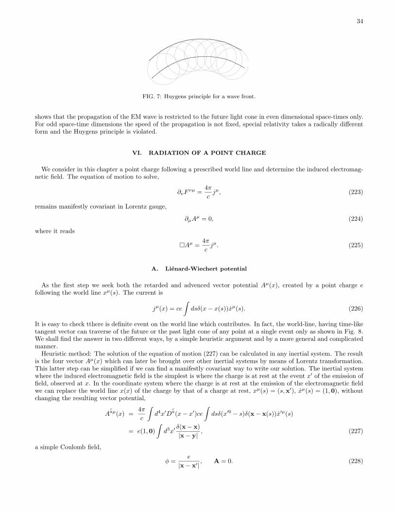
34

FIG. 7: Huygens principle for a wave front.

shows that the propagation of the EM wave is restricted to the future light cone in even dimensional space-times only.For odd space-time dimensions the speed of the propagation is not fixed, special relativity takes a radically differentform and the Huygens principle is violated.

VI. RADIATION OF A POINT CHARGE

We consider in this chapter a point charge following a prescribed world line and determine the induced electromag-netic field. The equation of motion to solve,

∂νFνµ =

4π

cjµ, (223)

remains manifestly covariant in Lorentz gauge,

∂µAµ = 0, (224)

where it reads

Aµ =4π

cjµ. (225)

A. Lienard-Wiechert potential

As the first step we seek both the retarded and advenced vector potential Aµ(x), created by a point charge efollowing the world line xµ(s). The current is

jµ(x) = ce

∫

dsδ(x− x(s))xµ(s). (226)

It is easy to check tthere is definite event on the world line which contributes. In fact, the world-line, having time-liketangent vector can traverse of the future or the past light cone of any point at a single event only as shown in Fig. 8.We shall find the answer in two different ways, by a simple heuristic argument and by a more general and complicatedmanner.Heuristic method: The solution of the equation of motion (227) can be calculated in any inertial system. The result

is the four vector Aµ(x) which can later be brought over other inertial systems by means of Lorentz transformation.This latter step can be simplified if we can find a manifestly covariant way to write our solution. The inertial systemwhere the induced electromagnetic field is the simplest is where the charge is at rest at the event x′ of the emission offield, observed at x. In the coordinate system where the charge is at rest at the emission of the electromagnetic fieldwe can replace the world line x(x) of the charge by that of a charge at rest, xµ(s) = (s,x′), xµ(s) = (1,0), withoutchanging the resulting vector potential,

Araµ(x) =

4π

c

∫

d4x′Dra(x− x′)ce

∫

dsδ(x′0 − s)δ(x− x(s))x′µ(s)

= e(1,0)

∫

d3x′ δ(x− x)

|x− y| , (227)

a simple Coulomb field,

φ =e

|x− x′| , A = 0. (228)

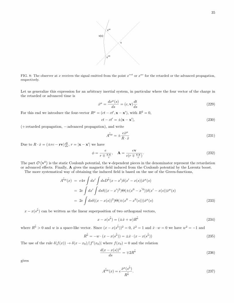
35

x(s)

x

x

xret

av

FIG. 8: The observer at x receives the signal emitted from the point xret or xav for the retarded or the advanced propagation,respectively.

Let us generalize this expression for an arbitrary inertial system, in particular where the four vector of the charge inthe retarded or advanced time is

xµ =dxµ(s)

ds= (c,v)

dt

ds(229)

For this end we introduce the four-vector Rµ = (ct− ct′,x− x′), with R2 = 0,

ct− ct′ = ±|x− x′|, (230)

(+:retarded propagation, −:advanced propagation), and write

Araµ = ± exµ

R · x (231)

Due to R · x = (±rc− rv) dtds , r = |x− x′| we have

φ =e

r ∓ r·vc

, A =ev

c(r ∓ r·vc )

. (232)

The part O(v0)is the static Coulomb potential, the v-dependent pieces in the denominator represent the retardation

or advanced effects. Finally, A gives the magnetic field induced from the Coulomb potential by the Lorentz boost.The more systematical way of obtaining the induced field is based on the use of the Green-functions,

Araµ(x) = e4π

∫

dx′

∫

dsDra(x− x′)δ(x′ − x(s))xµ(s)

= 2e

∫

dx′

∫

dsδ((x− x′)2)Θ(±(x0 − x′0))δ(x′ − x(s))xµ(s)

= 2e

∫

dsδ((x− x(s))2)Θ(±(x0 − x0(s)))xµ(s) (233)

x− x(sra) can be written as the linear superposition of two orthogonal vectors,

x− x(sra) = (±x+ w)R

ra (234)

where Rra > 0 and w is a space-like vector. Since (x− x(s

ra))2 = 0, x2 = 1 and x · w = 0 we have w2 = −1 and

Rra = −w · (x− x(s

ra)) = ±x · (x− x(s

ra)) (235)

The use of the rule δ(f(x))→ δ(x− x0)/|f ′(x0)| where f(x0) = 0 and the relation

d(x− x(s))2

ds= ∓2R

ra (236)

gives

Araµ(x) = e

xµ(sra)

Rra

. (237)

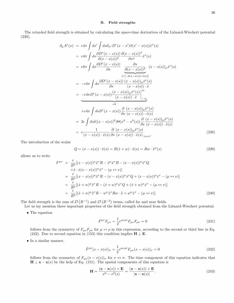
36

B. Field strengths

The retarded field strength is obtained by calculating the space-time derivatives of the Lienard-Wiechert potential(239),

∂µAν(x) = e4π

∫

dx′

∫

ds∂xµDr(x− x′)δ(x′ − x(s))xν(s)

= e4π

∫

ds∂Dr(x− x(s))

∂(x− x(s))2∂(x− x(s))2

∂xµxν(s)

= e8π

∫

ds∂Dr(x− x(s))

∂s

∂s

∂(x− x(s))2︸ ︷︷ ︸

1/[−2(x−x(s))·x(s)]

(x− x(s))µxν(s)

= −e4π∫

ds∂Dr(x− x(s))

∂s

(x− x(s))µxν(s)

(x− x(s)) · x

= −e4πDr(x− x(s))(x− x(s))µx

ν(s)

(x− x(s)) · x

∣∣∣∣

∞

−∞︸ ︷︷ ︸

=0

+e4π

∫

dsDr(x− x(s))∂

∂s

(x− x(s))µxν(s)

(x− x(s)) · x(s)

= 2e

∫

dsδ((x− x(s))2)Θ(x0 − x0(s))∂

∂s

(x− x(s))µxν(s)

(x− x(s)) · x(s)

= e1

(x− x(s)) · x(s)∂

∂s

(x− x(s))µxν(s)

(x− x(s)) · x(s) |s=sr(238)

The introduction of the scalar

Q = (x− x(s)) · x(s) = R(x+ w) · x(s) = Rw · xµ(s) (239)

allows us to write

Fµν =e

R3[(x− x(s))µxνR− xµxνR− (x− x(s))µxνQ

+x · x(x− x(s))µxν − (µ↔ ν)]

=e

R3[(x− x(s))µxνR− (x− x(s))µxνQ+ (x− x(s))µxν − (µ↔ ν)]

=e

R2[(x+ w)µxνR− (x+ w)µxνQ+ (x+ w)µxν − (µ↔ ν)]

=e

R2[(x+ w)µxνR− wµxνRw · x+ wµxν − (µ↔ ν)] (240)

The field strength is the sum of O(R−1

)and O

(R−2

)terms, called far and near fields.

Let us lay mention three important properties of the field strength obtained from the Lienard-Wiechert potential.

• The equation

FµνFµν =1

2ǫµνρσFµνFρσ = 0 (241)

follows from the symmetry of FµνFρσ for µ↔ ρ in this expression, according to the second or third line in Eq.(242). Due to second equation in (153) this condition implies H ⊥ E.

• In a similar manner,

F ρσ(x− x(s))σ =1

2ǫµνρσFµν(x− x(s))σ = 0 (242)

follows from the symmetry of Fµν(x − x(s))σ for ν ↔ σ. The time component of this equation indicates thatH ⊥ x− x(s) by the help of Eq. (151). The spatial components of this equation is

H =(x− x(s))×E

x0 − x0(s)=

(x− x(s))×E

|x− x(s)| . (243)

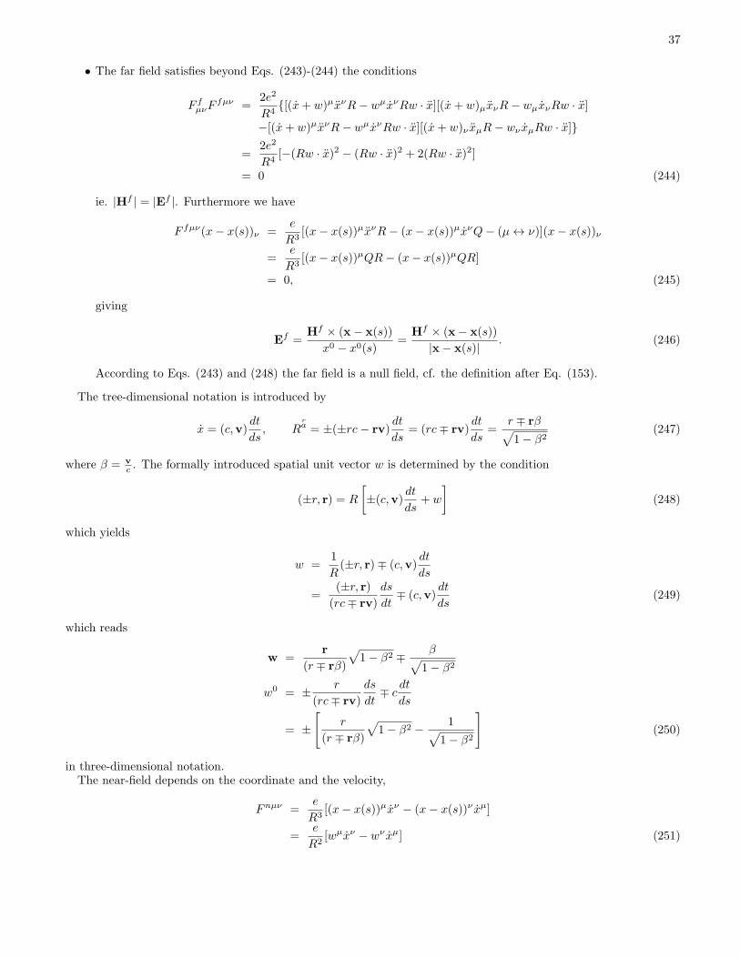
37

• The far field satisfies beyond Eqs. (243)-(244) the conditions

F fµνF

fµν =2e2

R4[(x+ w)µxνR− wµxνRw · x][(x+ w)µxνR− wµxνRw · x]

−[(x+ w)µxνR− wµxνRw · x][(x+ w)ν xµR− wν xµRw · x]

=2e2

R4[−(Rw · x)2 − (Rw · x)2 + 2(Rw · x)2]

= 0 (244)

ie. |Hf | = |Ef |. Furthermore we have

F fµν(x− x(s))ν =e

R3[(x− x(s))µxνR− (x− x(s))µxνQ− (µ↔ ν)](x− x(s))ν

=e

R3[(x− x(s))µQR− (x− x(s))µQR]

= 0, (245)

giving

Ef =Hf × (x− x(s))

x0 − x0(s)=

Hf × (x− x(s))

|x− x(s)| . (246)

According to Eqs. (243) and (248) the far field is a null field, cf. the definition after Eq. (153).

The tree-dimensional notation is introduced by

x = (c,v)dt

ds, R

ra = ±(±rc− rv)

dt

ds= (rc∓ rv)

dt

ds=

r ∓ rβ√

1− β2(247)

where β = v

c . The formally introduced spatial unit vector w is determined by the condition

(±r, r) = R

[

±(c,v) dtds

+ w

]

(248)

which yields

w =1

R(±r, r)∓ (c,v)

dt

ds

=(±r, r)

(rc∓ rv)

ds

dt∓ (c,v)

dt

ds(249)

which reads

w =r

(r ∓ rβ)

√

1− β2 ∓ β√

1− β2

w0 = ± r

(rc∓ rv)

ds

dt∓ c

dt

ds

= ±[

r

(r ∓ rβ)

√

1− β2 − 1√

1− β2

]

(250)

in three-dimensional notation.The near-field depends on the coordinate and the velocity,

Fnµν =e

R3[(x− x(s))µxν − (x− x(s))ν xµ]

=e

R2[wµxν − wν xµ] (251)

38

The near electric field, Ej = F j0, is

En =e

R2[wx0 − w0x]

=e(1− β2)

(r ∓ rβ)2

[(

r

(r ∓ rβ)

√

1− β2 ∓ β√

1− β2

)

1√

1− β2

∓(

r

(r ∓ rβ)

√

1− β2 − 1√

1− β2

)

β√

1− β2

]

=e(1− β2)

(r ∓ rβ)2

[(r

(r ∓ rβ)∓ β

1− β2

)

∓(

r

(r ∓ rβ)− 1

1− β2

)

β

]

=e(1− β2)

(r ∓ rβ)2

(r

(r ∓ rβ)∓ rβ

(r ∓ rβ)

)

= e(1− β2)(r∓ rβ)

(r ∓ r · β)3

= e(1− v2

c2 )(r∓ r v

c )

(r ∓ r·vc )3

(252)

The far-field depends on the acceleration as well,

F fµν =e

R3[(x− x(s))µ(xνR− xνQ)− (x− x(s))ν(xµR− xµQ)] (253)

and

Ef = er× [(r− r v

c )× a]

c2(r − r·vc )3

, (254)

where a = dvdt . The near and far magnetic fields can be obtained by using the relation (245).

C. Dipole radiation

The complications in obtaining the Lienard-Wiechert potential come from the retardation. Thus it is advised tosee the limits when the retardation effects are weak and the final result can be expanded in them. Let us supposethat the characteristic time and distance scales of the prescribed charge distribution are tch and rch, respectively. Theperiod length of the radiation is approximately tch, yielding the wavelength λ = ctch. The retardation time is whatneeds for the EM wave to traverse the charge distribution, tret = rch/c. The retardation effects are therefore weakfor tret/tch ≪ 1 which gives rch ≪ λ. Another way to express this inequality is to consider the characteristic speedof the charge system, vch = rch/tch, to write λ = crch/vch which yields vch ≪ c.

We assume that these inequalities hold and consider the leading order effect of the retardation on the retardedLienard-Wiechert potential (239)

Aµ(x) =∑

a

eaxµ(sra)

Rra

. (255)

It is sufficient to find the magnetic field,

A(x) =1

cr

∑

a

eava

(

1 +O( |v|

c

))

(256)

where r denotes the distance between the observation point and the center of the charges and va stands for thevelocity of the charge a at the time of observation. Since

∑

a

eava =d

dt

∑

a

eaxa =d

dtd (257)

39

where d is the dipole moment of the charge system we have

A(x) =1

cr

dd

dt(258)

in the leading order. Then the magnetic field is given by

H = ∇× 1

cr

dd(t− rc )

dt

= − 1

cr3r× dd

dt− 1

c2r2r× d2d

dt2

=1

cr3

∑

a

eava × r+1

c2r2

∑

a

eaaa × r (259)

the sum of the near and the far dipole fields. According to Eq. (248)

Ef =Hf × r

r=

1

c2r3

∑

a

ea(aa × r)× r. (260)

The far field, dipole radiation depends on the acceleration of the charges only.The radiation power passing trough a surface df is

dI = Sdf (261)

where S is the Poynting vector and is given by

dI =c

4πH2r2dΩ (262)

according to Eq. (181) where dΩ denotes the solid angle. In the case of the far dipole radiation we find

dI =1

4πc3r2

(d2d

dt2× r

)2

dΩ =1

4πc3

(d2d

dt2

)2

sin2 θdΩ (263)

where θ is the angle between d2

dt2d and r. The total radiated power is obtained by integrating over the solid angle,

I =

∫

dφ

∫

d(cos θ)1

4πc3

(d2d

dt2

)2

sin2 θ =2

3c3

(d2d

dt2

)2

. (264)

Note that had the near field been retaind in the expresion of the radiated power it would have dropped out in thelimit r → ∞, reflecting the fact that the near field belongs to the charge and it is only the far field which decouplesand decomes a new dynamical degree of freedom as will be shown below in Section VID. For a single charge we have

I =2e2a2

3c3. (265)

(J. Larmor, 1897).As a simple excercise let us estimate the energy loss of an electron on an orbit around the proton according to

classical physics. We can consider the motion of the electron in the (x, y) plane producing a time dependent dipole

d(t) = ea0

(cosωtsinωt

)

, (266)

a0 = ~2/me2 being the Bohr radius and the use of Eq. (266) gives

I =2ω4e2a20

3c3. (267)

By assuming a ballance between the centrifugal and the Coulomb forces, mrω2 = e2/r2 we can write

I =2e6

3m2a40c3∼ 109Ry/sec, (268)

indicating that the Hydrogen atom would loose stability and the electron would fall onto the proton in 10−9secaccording to classical physics.

40

D. Radiated energy-momentum

As a preparation for the reaction force acting on charges let us establish the energy-momentum balance for a pointcharge. For this end we need the field generated by the charge at large distances where the radiation field dominates.Hence we start by identifying some important properties of the radiation field.

The far field is null-field, therefore its energy-momentum tensor is

T fµν =1

4πF fµσF fν

σ

=e2

4πR6[(x− x(s))µ(xσR− xσQ)− (x− x(s))σ(xµR− xµQ)]

×[(x− x(s))σ(xνR− xνQ)− (x− x(s))ν(xσR− xσQ)]. (269)

Due to (x− x(s))2 = 0 we have

T fµν =e2

4πR6[(x− x(s))µ(xνR− xνQ)(xR− xQ) · (x− x(s))

−(x− x(s))µ(x− x(s))ν(xR− xQ)2

+(xµR− xµQ)(x− x(s))ν(x− x(s)) · (xR− xQ)]. (270)

The first and the last terms contain the same scalar product which is actually vanishing,

(xR− xQ) · (x− x(s)) = [x x · (x− x(s))︸ ︷︷ ︸

R

−x x · (x− x(s))︸ ︷︷ ︸

Q

] · (x− x(s))

= [x · (x− x(s)][x · (x− x(s))]

−[x · (x− x(s))][x · (x− x(s))] = 0, (271)

therefore we can write

T fµν = − e2

4πR6(x− x(s))µ(x− x(s))ν(xR− xQ)2

= − e2

4πR6(x− x(s))µ(x− x(s))ν(x2R2 +Q2) (272)

where the orthogonality x · x = 0 was used in the last equation.The radiation reaction four-force acting on the charge, Kµ = −∂νT νµ, can be obtained by considering the integral

I of ∂νTνµ over the four-volume V of Fig. 9, bounded by the hyper-surfaces S1, C1, S2, C2. For sufficiently far from

the charges the far field survives only and we have

I =

∫

dV ∂νTνµ

=

∫

∂V

dSνTνµ

=

∫

S2

dSνTνµ −

∫

S1

dSνTνµ +

∫

C1

dSνTνµ +

∫

C2

dSνTνµ (273)

for the far field contributions. The last two terms are vanishing because T fνµ ≈ (x − x(s))ν , dSνTνµ = 0, the

energy-momentum flux does not cross the hyper-surfaces C1 and C2. It is important to note that this is not true forthe near field because Tnµν 6≈ (x − x(s))ν , the near-field, eg. Coulomb field moves with the charge. The co-movingnature of the near-field contrasted with the decoupled, freely propagating nature of the far field which identifies theradiation field.Since the energy-momentum tensor tµν of the localized charge is vanishing in the integration volume the energy-

momentum conservation ∂ν(Tνµ + tνµ) = 0 assures I = 0, and

∆Pµ = −∫

S

dSνTfνµ, (274)

the radiated energy-momentum, is a four-vector and is independent of the choice of the surface S.

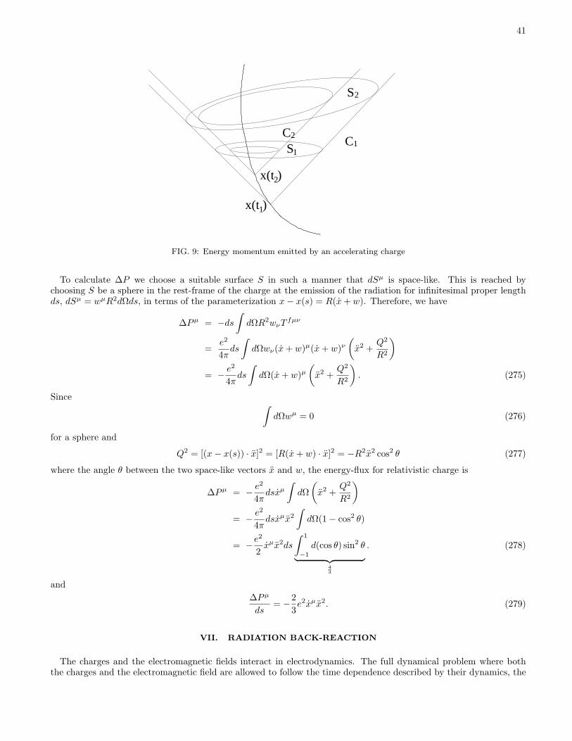
41

x(t )2

x(t )1

S

SC

2

1

C21

FIG. 9: Energy momentum emitted by an accelerating charge

To calculate ∆P we choose a suitable surface S in such a manner that dSµ is space-like. This is reached bychoosing S be a sphere in the rest-frame of the charge at the emission of the radiation for infinitesimal proper lengthds, dSµ = wµR2dΩds, in terms of the parameterization x− x(s) = R(x+ w). Therefore, we have

∆Pµ = −ds∫

dΩR2wνTfµν

=e2

4πds

∫

dΩwν(x+ w)µ(x+ w)ν(

x2 +Q2

R2

)

= − e2

4πds

∫

dΩ(x+ w)µ(

x2 +Q2

R2

)

. (275)

Since∫

dΩwµ = 0 (276)

for a sphere and

Q2 = [(x− x(s)) · x]2 = [R(x+ w) · x]2 = −R2x2 cos2 θ (277)

where the angle θ between the two space-like vectors x and w, the energy-flux for relativistic charge is

∆Pµ = − e2

4πdsxµ

∫

dΩ

(

x2 +Q2

R2

)

= − e2

4πdsxµx2

∫

dΩ(1− cos2 θ)

= −e2

2xµx2ds

∫ 1

−1

d(cos θ) sin2 θ

︸ ︷︷ ︸43

. (278)

and

∆Pµ

ds= −2

3e2xµx2. (279)

VII. RADIATION BACK-REACTION

The charges and the electromagnetic fields interact in electrodynamics. The full dynamical problem where boththe charges and the electromagnetic field are allowed to follow the time dependence described by their dynamics, the

42

mechanical equation of motion and the Maxwell equations is quite a wonderful mathematical problem. A simplerquestion is when the motion is partially restricted, when one members of this system is forced to follow a prescribedtime dependence and the other is allowed to follow its own dynamics only. For instance, the world lines of a pointcharge moving in the presence of a fixed electromagnetic field can easily be found by integrating the equation of motion(133). The use of the Green functions provides the solution for a number or engineering problems in electrodynamicswhere the electromagnetic fields are sought for a given charge distribution. We devote this chapter to a questionwhose complexity is in between the full and the restricted dynamical problems but appears a more fundamental issue.

A. The problem

Let us consider a charge moving under the influence of a nonvanishing external force. The force accelerates it andin turn radiation is emitted. The radiation has some energy and momentum which is lost in the supposedly infinitespace surrounding the charge. Thus the energy and momentum of our charge is changed and we have to assume thatthere is some additional force acting on the charge.The very question is rather perplexing because one would have thought that the equation of motion for the charge,

Eq. (133), containing the Lorentz force, the second term on the right hand side is the last word in this issue. Thereis apparently another force in the ”true” equation of motion! The complexity of this problem explains that this isperhaps the last open chapter of classical electrodynamics.There is a further, even more disturbing question. Does a point-like charge interact with the electromagnetic field

induced by its own motion? It is better not, otherwise we run into the problem of singularities like a point-charge atrest at the singular point of its own Coulomb-field. But the electric energy of a given static charge distribution ρ(x),

E =1

2

∫

d3xd3yρ(x)ρ(y)

|x− y| (280)

suggests that the answer is affirmative.The radiation reaction force whose derivation is the goal of this chapter touches a number of subtle issues.

1. Singular solutions: Is there regular solutions at all for the set of coupled equations for point charges and theelectromagnetic field? It may happen that some smearing, provided by the unavoidable vacuum polarization ofquantum electrodynamics is needed to render the solution of the classical equations of motion regular.

2. Lack of variation principle: The existence of the radiation back reaction force is beyond doubt but itsderivation is non-trivial. It is a friction force, describing the loss of energy to the radiation field, and can notbe derived by variational principle ie. it is not present in the usual variational system of equations of motion ofclassical electrodynamics.

3. Breakdown of time reversal invariance: The energy radiated out by the charge can not be recoveredanymore in an infinite system. Thus the sign of the radiation reaction force represents a dynamical breakdownof the time inversion invariance of the basic laws of electrodynamics.

4. Loss of causal structure: The radiation back reaction force acting on point charges can be calculated exactlyand turns out to be proportional to the third derivative of the coordinates. Such kind of force generates acausal,advanced effects and lead to self-accelerating motion.

5. Limit of classical physics The self interaction of a point charge is a singular problem, it can be made sensein some limit only, when the size of a finite, extended charge distribution is sent to zero. It reveals an ill definedcorner of classical electrodynamics , a pillar of ninteenth century classical physics. Had the physicist missed thediscovery of the quantum world they would have been forced to face the challenge of modifying the fundamentallaws in physics to render classical electrodynamics of point charges consistent. The only counterpart of such aclear sign of the end of applicability of the classical rules is the Gibbs paradox in statistical phyics.

6. Noncommuting limits: The problem about the limit r0 → 0 where r0 is the characteristic size of the chargedistribution of a particle raises the possibility that the limits ~ → 0 and r0 → 0 do not commute. In fact, indiscussing a point charge in classical electrodynamics one tacitly takes the limit ~ → 0 first to get the lawsof classical electrodynamics where the limit r0 → 0 is performed at the end. But a strongly localized particleinduces quantum effects what should be taken into account by keeping ~ finite, ie. we should start with thelimit r0 → 0 to introduce a point-like particle in Quantum Mechanics and the classical limit ~ → 0, should beperformed at the end only. There are no point charges in this scheme because even if one starts with a strictlypoint-like charge the unavoidable vacuum-polarization effect generates a charge density polarization cloud ofthe size of the Compton wavelength around the point charge.

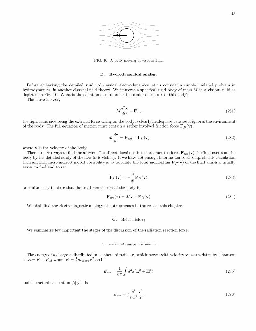
43

V

FIG. 10: A body moving in viscous fluid.

B. Hydrodynamical analogy

Before embarking the detailed study of classical electrodynamics let us consider a simpler, related problem inhydrodynamics, in another classical field theory. We immerse a spherical rigid body of mass M in a viscous fluid asdepicted in Fig. 10. What is the equation of motion for the center of mass x of this body?

The naive answer,

Md2x

dt2= Fext (281)

the right hand side being the external force acting on the body is clearly inadequate because it ignores the environmentof the body. The full equation of motion must contain a rather involved friction force Ffl(v),

Mdv

dt= Fext + Ffl(v) (282)

where v is the velocity of the body.There are two ways to find the answer. The direct, local one is to construct the force Fext(v) the fluid exerts on the

body by the detailed study of the flow in is vicinity. If we have not enough information to accomplish this calculationthen another, more indirect global possibility is to calculate the total momentum Pfl(v) of the fluid which is usuallyeasier to find and to set

Ffl(v) = −d

dtPfl(v), (283)

or equivalently to state that the total momentum of the body is

Ptot(v) = Mv +Pfl(v). (284)

We shall find the electromagnetic analogy of both schemes in the rest of this chapter.

C. Brief history

We summarize few important the stages of the discussion of the radiation reaction force.

1. Extended charge distribution

The energy of a charge e distributed in a sphere of radius r0 which moves with velocity v, was written by Thomsonas E = K + Eed where K = 1

2mmechv2 and

Eem =1

8π

∫

d3x(E2 +H2), (285)

and the actual calculation [5] yields

Eem = fe2

r0c2v2

2, (286)

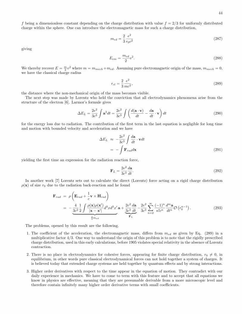
44

f being a dimensionless constant depending on the charge distribution with value f = 2/3 for uniformly distributedcharge within the sphere. One can introduce the electromagnetic mass for such a charge distribution,

med =2

3

e2

r0c2(287)

giving

Eem =med

2v2. (288)

We thereby recover E = m2 v

2 where m = mmech+med. Assuming pure electromagnetic origin of the mass, mmech = 0,we have the classical charge radius

rcl =2

3

e2

mc2, (289)

the distance where the non-mechanical origin of the mass becomes visible.The next step was made by Lorentz who held the conviction that all electrodynamics phenomena arise from the

structure of the electron [6]. Larmor’s formule gives

∆EL =2e2

3c3

∫

a2dt =2e2

3c3

∫ (d(a · v)

dt− da

dt· v)

dt (290)

for the energy loss due to radiation. The contribution of the first term in the last equation is negligible for long timeand motion with bounded velocity and acceleration and we have

∆EL ≈ −2e2

3c3

∫da

dt· vdt

= −∫

Fraddx (291)

yielding the first time an expression for the radiation reaction force,

FL =2e2

3c3da

dt. (292)

In another work [7] Lorentz sets out to calculate the direct (Lorentz) force acting on a rigid charge distributionρ(x) of size r0 due to the radiation back-reaction and he found

Frad = ρ

(

Erad +1

cv ×Hrad

)

= − 4

3c21

2

∫ρ(x)ρ(x′)

|x− x′| d3xd3x′

︸ ︷︷ ︸43med

a+2e2

3c3da

dt︸ ︷︷ ︸

FL

−2e2

3c3

∞∑

n=2

(−1)nn!cn

dma

dtnO(rn−10

). (293)

The problems, opened by this result are the following.

1. The coefficient of the acceleration, the electromagnetic mass, differs from med as given by Eq. (289) in amultiplicative factor 4/3. One way to understand the origin of this problem is to note that the rigidly prescribedcharge distribution, used in this early calculations, before 1905 violates special relativity in the absence of Lorentzcontraction.

2. There is no place in electrodynamics for cohesive forces, appearing for finite charge distribution, r0 6= 0, inequilibrium, in other words pure classical electrodynamical forces can not hold together a system of charges. Itis believed today that extended charge systems are held together by quantum effects and by strong interactions.

3. Higher order derivatives with respect to the time appear in the equation of motion. They contradict with ourdaily experience in mechanics. We have to come to term with this feature and to accept that all equations weknow in physics are effective, meaning that they are presumable derivable from a more microscopic level andtherefore contain infinitely many higher order derivative terms with small coefficients.

45

4. The divergence med =∞ in the limit r0 → 0 spoils our ideas about point charges. The concept of point chargesis irrecovably removed from physics by the ultraviolet divergences appearing in quantum field theories.

While Lorentz concentrated on the energy loss of the charge system Abraham approached the problem from thepoint of view of the momentum loss. He identified the momentum of the Coulomb field of an charge in uniform motionby its Poyting’s vector [8],

prad =1

4πc

∫

(E×H)d3x. (294)

The actual calculation yields

prad =4

3medv (295)

where the electromagnetic mass is given by Eq. (289). The absence of Lorentz contraction lead to the factor 4/3again.Approximately in the same time Sommerfeld calculated the self force acting on a charge distribution ρ(x) in its

co-moving coordinate system by ignoring the higher order than linear terms in the acceleration and its time derivatives[9],

Frad =2e2

3c

∞∑

n=0

(−1)nn!

cndn+1

dctn+1v, (296)

where

cn =

∫

d3xd3yρ(x)|x− y|n−1ρ(y). (297)

He considered charges distributed homogeneously on the surface of a sphere of radius r0 when

cn =2(2r0)

n

n+ 1(298)

and managed to resum the series which results the non-relativistic equation of motion

mdv

dt= Fext +med

v(t− 2 r0c )− v(t)

2r0(299)

which is a finite difference equation with the delay time needed to reach the opposite points of the sphere.Soon after the discovery of special relativity Laue has found the relativistic extension of Lorentz’s result (294), [10]

mcxµ = −2

3e2(xµx2 +

...xµ), (300)

an equation to be derived in a more reliable manner later by Dirac. The first term is positive definite and representsthe breakdown of the time inversion invariance, the loss of energy due to the ’friction’ caused by the radiation. Thesecond, the so called Schott term can change sign and stands for the emission and absorption processes.

A particularly simple, phenomenological argument to arrive at the self force (302) [11] is based on the constraintx · x = 0 on the world line of a point particle which asserts that the four-force Fµ

rad = mmechxµ must be orthogonal

to the four-velocity. One can easily construct the linearized equation of motion, an orthogonal vector which is linearin the velocity and its derivatives by means of the projector

Pµν = gµν − xµxν (301)

as

Fµrad = Pµν

∞∑

n=1

andnxν(s)

dsn. (302)

The derivative of the constraint x · x = 0 with respect to the world-line parameter,

...x · x+ x2 = 0, (303)

46

gives for the self force truncated at the third derivative

mmechcxµ ≈ Pµν(a2x

ν + a3...x ν) = a2x

µ + a3(...xµ + xµx2). (304)

The mass renormalization m = mmech−a2 eliminates the first term on the right hand side and expresses the physicalmass as the sum of the mechanical and part and the contribution from electrodynamics. The comparison with Eq.(302) gives a3 = −2e2/3.The third derivative with respect to the time in the equation of motion presents a new problem, such an equation

has runaway, self-accelerating solution,

x0 = cosh[r0(es/r0 − 1)], x1 = sinh[r0(e

s/r0 − 1)], x2 = x3 = 0, (305)

with rc being the classical electron radius (291). This is unacceptable. Dirac proposed an additional boundarycondition in time for the charges which is needed for the equation of motion with third time derivative. This is to beimposed at the final time and it eliminates the runaway solutions. The problem which renders this proposal difficultto accept is that it generates acausal effects on the motion of the charges, acceleration before the application of theforces.The origin of this problem is the sharp boundary of the homogeneously distributed charge in a sphere when

the radius r0 tends to zero. It was shown that both the runaway and the preaccelerating solutions are absent forSommerfeld’s equation of motion (301) as long as r0 > rcl [12]. It is the truncated power series approximation forthis finite difference equation which creates the problem in the point charge limit.

2. Point charge limit

The singular nature of the point charge limit forced Dirac to avoid the use of the Lorentz-force, the second term inthe last equation of (133) altogether. Instead, he extracted the force by means of the energy-momentum conservationwhich can be applied safely, outside of the body [13]. His calculation is based on the introduction of a tube of radius r0around the world-line of the body which is supposed to include all charge and the calculation of the energy-momentumbalance equation for the charge-electromagnetic field interactive system. It turns out that the forces acting on thebody can be determined and are local in time when the limit r0 → 0 is taken. An important qualitative result of thisscheme can be summarized by means of the decomposition (217) of the retarded Green function. Dirac found thatthe the singular part of the force arises exclusively from the near field component of the induced field, An = 4π

c Dn · j.Furthermore, the remaining, far field component, Af = 4π

c Df ·j remains finite in the point charge limit and reproducesLaue’s result, Eq. (302). Based on theses results we follow here a shorter path to reach the goal [4], based on thedirect use of the Lorentz force, amended by a regularization of the singular generalized functions appearing in thepoint charge limit.We start with

Fµνrad(s

′) = 4πe

∫

dsDrad(x− x′)d

ds

(x− x(s))µxν(s)

(x− x(s)) · x(s) − (µ←→ ν), (306)

where

Drad(x) = Dr(x− x′)−Da(x− x′) =1

2πǫ(x0 − x

′0)δ((x− x′)2). (307)

We write s = s′ + u and expand in u,

x(s)− x(s′) = ux+u2

2x+

u3

6

d3x

ds3+ · · ·

x(s) = x+ ux+u2

2

d3x

ds3+ · · ·

(x(s)− x(s′))2 = u2 +O(u4)

(x(s)− x(s′)) · x = u+O(u3)

ǫ(x0(s)− x′0(s′)) = ǫ(u) (308)

47

to find

Fµνrad(s

′) = 2e

∫

dsǫ(u)

×δ(u2)d

du

[(

x+u

2x+

u2

6

d3x

ds3

)µ(

x+ ux+u2

2

d3x

ds3

)ν]

−(µ←→ ν) (309)

= 2e

∫

duǫ(u)δ(u2)

d

du

(

uxµxν +u

2xµxν +

u2

2xµ dx

ν

ds3+

u2

6

dxµ

ds3xν

)

− (µ←→ ν).

The small but finite size of the charge compared with the width of the light cone where the radiation field is constrainedis taken into account by the formal steps

δ(u2) = limv→0+

δ(u2 − v2) = limv→0+

[δ(u− v)

2v+

δ(u+ v)

2v

]

(310)

and

ǫ(u)δ(u2) = limv→0+

[δ(u− v)

2v− δ(u+ v)

2v

]

= −δ′(u), (311)

yielding

Fµνrad(s

′) = 2e

∫

duδ(u)d2

du2

(u

2xµxν +

u2

3xµ dx

ν

ds3

)

− (µ←→ ν)

=4

3e

(

xµ d3xν

ds3− xν d

3xµ

ds3

)

(312)

and

Kµreact = mcxµ

rad(x′) =

e

2cFµνrad(x

′)xν

=2

3e2(xµ...x · x− ...

xµ). (313)

Finally, by the the use of Eq. (305) we recover Eq. (302). The regularization of the product of two distributions inEq. (313) is the delicate point, justified by the recovery of Dirac’s result.

The near field represents no loss or gain in energy and momentum, it rather enriches the structure of the chargeby modifying, renormalizing its free equation of motion. Dirac found that Lorentz’s divergent mreact is given by thenear-field and gives rise a mass renormalization. To see this we start with the action

S = −mbc

∫

ds+ Sed

Sed = −e

c

∫

d4xAν(x)jν(x)

= −e

2

∫

d4x[Arν(x) +Aa

ν(x)]

∫

ds ρ(x− x(s))︸ ︷︷ ︸

form factor

xν(s) (314)

We write the near field Anν (x) =

12 [A

rν(x) +Aa

ν(x)] as

Anν (x) = 4πe

∫

d4x′ds′1

2[Dr(x− x′) +Dadv(x− x′)]ρ(x′ − x(s′))xν(s

′)

= e

∫

d4x′ds′δ((x− x′)2)ρ(x′ − x(s′))xν(s′) (315)

48

which yields, upon inserted into the action

Sed = −e2∫

d4xd4x′dsds′δ((x− x′)2)ρ(x′ − x(s′))ρ(x− x(s))x(s′) · x(s)

= −e2∫

d4wd4w′dsds′

×δ((w − w′ + x(s)− x(s′))2)ρ(w′)ρ(w)x(s′) · x(s).(316)

This was the decisive step, this action does not contain the Lienard-Wiechert potentials anymore, the Green functionswere used to eliminate the electromagnetic field from the problem by means of their equations of motion. We followthe limit r0 →, s′ = s+ u, x(s′) = x+ ux+ · · · , x(s)− x(s′) = −ux+ · · · and write

Sed ≈ −e2∫

dsd4wd4w′duδ((w − w′ − ux)2)ρ(w′)ρ(w)

= −e2

2

∫

dsd4wd4w′

×[

1

(w − w′ − uretx) · x+

1

(w − w′ − uadvx) · x

]

ρ(w′)ρ(w)

= −e2

2

∫

dsd4wd4w′

×[

1

(w − w′) · x− uret+

1

(w − w′) · x− uadv

]

ρ(w′)ρ(w)

= −medc

∫

ds (317)

where the integral in the third equation diverges and becomes independent of s when ρ(x)→ δ4(x) and

med =e2

2c

∫

d4wd4w′

[1

(w − w′) · x− uret+

1

(w − w′) · x− uadv

]

ρ(w′)ρ(w) (318)

What is found is a renormalization of the mass, the combination mph = mb + mel is observable only which setsmb = mph −med.

3. Iterative solution

The coupled equations of motion for the charge and the electromagnetic field can be solved iteratively, by reinsertingthe Lienard-Wiechert potential obtained by means of the solution of the mechanical equation [2]. They set up aperturbation expansion in the retardation which comprises the nontrivial effects of the radiation and obtain theradiation force in two steps. First they calculate the effective Lagrangian for the charge, obtained by eliminatingthe electromagnetic field by the Maxwell equation in order O (v/c). The next order contain the radiational frictionforce and is obtained by iterating the equation of motion. It is reassuring to see that the further iterations in theretardation yield vanishing result in the point charge limit.The retarded Lienard-Wiechert potential (which can not be obtained from an action principle due to its non time

reflection symmetrical form) leads to the effective Lagrangian

L = −∑

a

mac2

√

1− v2ac2−∑

a

eaφ+∑

a

eacA · va

=∑

a

[mav

2a

2+

mav4a

8c2+O

(v6

c6

)]

−∑

a

ea

∫

d3x′ ρ(t−|xa−x

′|c ,x′)

|xa − x′|

+∑

a

eac2

∫

d3x′ j(t−|xa−x

′|c ,x′)

|xa − x′| · va (319)

for a system of charges when the self-interaction is retained.

49

We make an expansion in the retardation by assuming v ≪ c, R/c ≪ τ , τ being the characteristic time scale of

the charges. Note that the factor |xa − x′|n in the higher, O(

( v2

c2 )n)

order contributions with n ≥ 3 suppresses the

singularity at |xa − x′| = 0. We find

φ(t, ra) =∑

b

[∫

drbρ(t, rb)

Rab− 1

c∂t

∫

drbρ(t, rb)

︸ ︷︷ ︸

Q=const.

+1

2c2∂2t

∫

drbRabρ(t, rb)

− 1

6c3∂3t

∫

drbR2abρ(t, rb)

]

+O(

1

c4

)

A(t, ra) =∑

b

[1

c

∫

drbj(t, rb)

Rab− 1

c2∂t

∫

drbj(t, rb)

]

+O(

1

c3

)

, (320)

what yields

φa =∑

b

[ebRab

+eb2c2

∂2tRab −

eb6c3

∂3tR

2ab

]

Aa =∑

b

[ebvb

cRab− eb

c2∂tvb

]

(321)

in the point charge limit. We perform the gauge transformation

φ′a = φa −

1

c

∑

b

[

∂t

( eb2c

∂tRab −eb6c2

∂2tR

2ab

)]

=∑

b

ebRab

= φ′(0)a

A′a = Aa +∇

∑

b

[( eb2c

∂tRab −eb6c2

∂2tR

2ab

)]

=∑

b

ebvb

cRab− eb

c2∂tvb +

eb2c∇∂tRab −

eb6c2

∂2t ∇R2

ab︸ ︷︷ ︸

2Rab

= A′(1)

a +A′(2)a . (322)

The Lagrangian is

L(0) =∑

a

mav2a

2− 1

2

∑

a 6=b

eaebRab

(323)

in the non-relativistic limit, O(( vc )

0)after ignoring an unimportant, diverging self energy for a = b.

For the next non-relativistic order, O(vc

), we need

∇∂tR = ∂t∇R = ∂tn =∂tR

R− R∂tR

R2(324)

where n = (r−r′)/|r−r′| denotes the unit vector from the charge to the observation point and R∂tR = R∂tR = −Rv,with

∂tn =−v + n(n · v)

R. (325)

One finds

φ′(0)a =

∑

b

ebRab

A′(1)a =

∑

b

ebvb + nb(nb · vb)

2cRab(326)

and the Lagrangian is

L(2) =∑

a

(mav

2a

2+

mav4a

8c2

)

(327)

−1

2

∑

a 6=b

eaebRab

+1

2

∑

a 6=b

eaebc2Rab

[va · vb + (va · nab)(vb · nab)]

50

in this order after a diverging self energy is ignored again for a = b.The next, O

(( vc )

2)order electromagnetic field contains the radiation induced friction force and can not be repre-

sented in the Lagrangian. We set R = r− r′, ∂tR = −∂tr′ and write

A′(2)a =

∑

b

[ebc2

∂tvb +eb3c2

∂tvb

]

= −∑

b

2

3

ebc2

∂tvb. (328)

In the absence of explicit x-dependence the magnetic field is vanishing in this order, H(2) = 0. The force acting onthe charge is of electric origin alone and the self force arises from the electric field

E(2)a = −1

c∂tA

′(2)a −∇ φ(2)

a︸︷︷︸

=0

=2

3

ea∂3t xa

c3(329)

The energy loss per unit time is

W =∑

a

Fa · va

=3

2

1

c3

∑

b

eb∂3t xb ·

∑

a

ea∂txa

=3

2

1

c3

∑

ab

eaeb[∂t(∂2t xb · ∂txa)− (∂2

t xa · ∂2t xb)] (330)

with the time average

W = −3

2

1

c3

∑

ab

eaeb(∂2t xa · ∂2

t xb) (331)

where the total derivative term can be neglected.The higher order contributions in the retardation become negligible in the point-like charge limit when R→ 0 and

the expression for the radiation reaction force

Frr =2

3

e2∂2t v

c3(332)

becomes exact! We see that we recover the second term in the right hand side of the last equation of Eqs. (302) butnot the first one in this manner, by relying on the retarded potentials.

The non-relativistic equation of motion,

m∂tv =2

3

e2∂2t v

c3(333)

leads unavoidable to the runaway solution

∂tv = v0et 32

mc3

e2 . (334)

The equation of motion with the Lorentz-force, corrected by the radiation reaction is

m∂tv = eEext +e

cv ×Hext +

2

3

e2∂2t v

c3. (335)

We arrived finally at a central question: at what length scales can we see the radiation reaction forces? Thecondition for the radiation back-reaction be small and an iterative solution is applicable is the following. In the restframe

∂2t v =

e

m∂tEext +

e

mc∂tv ×Hext +O

(c−3). (336)

51

Since ∂tv = eEext/m,

∂2t v =

e

m∂tEext +

e2

m2cEext ×Hext +O

(c−3)

(337)

and the radiation reaction force is

Frr =2

3

e3

mc3∂tEext

︸ ︷︷ ︸

O(

e3ωmc3

E)

+2

3

e4

m2c4Eext ×Hext

︸ ︷︷ ︸

O(

e4

m2c4EH

)

+O(c−5). (338)

The first term is negligible compared with the force generated by the external electric field for a monochromaticfield with frequency ω if

|Frr||Fext|

≈ e2ω

mc3≪ 1 (339)

or

e2

mc2≪ c

ω=

λ

2π. (340)

Thus classical electrodynamics becomes inconsistent due to pair creations at distances shorter than the classical chargeradius, ℓ ≈ λC = e2/mc2.We note that the second term is negligible,

H ≪ m2c4

e3(341)

for realistic magnetic fields.

4. Action-at-a-distance

A different approach to electrodynamics which might be called effective theory in the contemporary jargon is basedon the elimination of the electromagnetic field altogether from the theory [14–16].Let us write the action of a system of charges described by their world lines xµ

a(s) and the electromagnetic field ina condensed notation as

S =∑

a

Sm[xa] +1

2A ·D−1 ·A−

∑

a

ja ·A (342)

where the dot stands for space-time integration and index summation, j · A =∫dxjµ(x)Aµ(x), etc. The Maxwell

equation, δSδA = 0, yields

A = D · j. (343)

This equation can be used to eliminate A from the action and to construct the effective theory for the charges withthe action

S =∑

a

Sm[xa] +1

2

∑

ab

ja ·D ·D−1 ·D · jb −∑

ab

ja ·D · jb

=∑

a

Sm[xa]−1

2

∑

ab

ja ·D−1 · jb

→∑

a

Sm[xa]−1

2

∑

a 6=b

ja ·D−1 · jb (344)

without the electromagnetic field. The elimination of the field degrees of freedom generates action-at-a-distance. Theself-interaction was omitted in the last equation.

52

The Maxwell equation indicates that D should be a Green-function. But which one? According to Dirac’s proposalwe have near and far field Green-functions

An

f =1

2(Ar ±Aa) =

1

2(Dr ±Da) · j (345)

which motivates the notation Dn

f = 12 (D

r ±Da). Whatever Green-function we use, the symmetric part survives only

because A ·B ·A = 0 for an anti-symmetrical operator, Btr = −B. Since Da(x, y) = Dr(y, x), Dn and Df are just thesymmetric and antisymmetric part of the inhomogeneous propagator and we have to use Dn in the action principle.The self-interaction generated by the near-field and ignored in the last line of Eqs. (346) is indeed a world-lineindependent, divergent term.The support of the Green-function is the light-cone therefore the charge a at point xa interacts with the charge b

if the world-line xb(s) of the charge b pierces the light-cone erected at point xa. The interaction is governed by thenear-field Green-function and it is 50% retarded and 50% advanced. Such an even distribution of the retarded andadvanced interaction assures the formal time inversion invariance.The unwanted complication of the near-field mediated interactions is that it eliminates radiation field and the

retardation effects. It is a quite cumbersome procedure to add by hand the appropriate free field to the solution whichrestores the desired initial conditions.The use of the retarded Green-function assumes that the in-fields are weak. This is not the case for the out-fields

and the time inversion symmetry is broken. A sufficient plausible assumption to explain this phenomenon is theproposition that the Universe is completely absorptive, there is no electromagnetic radiation reaching spatial infinitiesdue to the elementary scattering processes of the inter-galactic dust [17]. The equation of motion for the charge a inthe theory given by the action (346),

mcxµa =

e

cFnµν xaν

=e

2c

∑

b 6=a

(F rµνb + F aµν

b )xaν (346)

can be written as

mcxµa =

e

c

∑

b 6=a

F rµνb +

1

2(F rµν

a − F aµνa )− 1

2

∑

b

(F rµνb − F aµν

b )

xaν . (347)

The first term represents the usual retarded interaction with the charges, self interactions ignored. The second termis the regular far field generated by the charge and provides the forces needed for the energy-momentum conservationfor radiating charges. The last expression, the radiation field of all charges is vanishing in a completely absorbingUniverse. The origin of the breakdown of the time reversal invariance needed for the appearance of the radiationfriction force which can be derived without difficulty from Eq. (349) is thus located in the absorbing nature ofthe Universe. Calculations performed in Quantum Electrodynamics in finite, flat space-time support the absorbingUniverse hypothesis.

5. Beyond electrodynamics

Similar radiation back-reaction problem exist in any interactive particle-field theory, for instance gravity or a moreacademic model where the interaction is mediated by a massive scalar field.

A mass curves the space-time around itself and is actually moves in such a distorted geometry. part of thedistortion is instantaneous, the analogy of the Coulomb force of electrodynamics, another part displays retardationand represents gravitational radiation. It was found [18, 19] that there is indeed a radiation back-reaction force ingravity and its additional feature is that it has a non-local component parallel to the four-acceleration, hence themass is renormalized by a term which depends on the whole past of the motion. It is the special vector algebrawhich rendered the mass renormalization a part and time independent constant in Eq. (289) for the electromagneticinteraction in flat space-time. But a conceptual issue which remains to settle in the gravitational case is that ingeneral any explicit use of the space-time coordinate corresponds to a gauge choice, in particular the form of the selfforce one can get is gauge dependent and not physical. The satisfactory solution of this problem which is still aheadof us is to translate all relevant dynamical issues into gauge invariant, coordinate choice independent form. The lossof the mass as a constant to characterize the motion of a point particle obviously forces radical changes upon our wayto imagine classical physics.

53

The origin of the non-local nature of the self-force can easily be understood. An external background curvatureacts as a mass term for the gravitational radiation. Therefore, the dynamical problem here is like the radiationback-reaction arising from interacting with a massive field. This problem can specially easily analyzed in the case ofa massive scalar field. Its retarded Green function is non-vanishing within the future light cone as opposed to themassless Green function whose support is the future light cone only. Therefore whole past of the world-line for thepoint x(s) lies within the past light cone of x(s) and contribute to the self-force as opposed to the simple situation ofthe massless electromagnetic interaction, depicted in Fig. 8.

D. Epilogue

The recent developments in High Energy Physics, namely the construction of effective theories based on the useof the renormalization group shows clearly the origin of the Abraham-Lorentz force. When degrees of freedom areeliminated in a dynamical system by means of their equation of motion then the equations of motion of the remainingdegrees of freedom change. The new terms represent the correlations realized by the eliminated degrees of freedomin the dynamics of the remaining part of the system. When the effect of the self field is considered on a charge thenwe actually eliminate the EM field and generate new pieces to the equations of motion for the charges. These are theradiation back-reaction forces, their importance can systematically be estimated by the method of the renormalizationgroup, applied either on the classic or the quantum level.It may happen that the coupled set of equations of motion for point charges and the electromagnetic field has no

regular solution and electrodynamics of point charges is well defined on the quantum level only. This is reminescentof the possibility that the proof of relaxation and the approach to an equilibrium ensemble in statistical physics mightneed quantum mechanics.

[1] J. D. Jackson, Classical Electrodynamics, John Wiley and Sons, New York.[2] L. D. Landau, E. M. Lifshitz, The Classical Theory of Fields, Vol2. (4th ed.) Butterworth-Heinemann.[3] F. Rohrlich, Classical Charged Particles, Addison-Wesley Publishing Co., Redwood City, (1965).[4] A. O. Barut, Electrodynamics and Classical Theory of Fields and Particles, The MacMillan Co., New York,1964.[5] J. J. Thomson, Phil. Mag. 11, 229 (1881).[6] H. A. Lorentz, Enzykl. Math. Wiss. V. 1, 188 (1903).[7] H. A. Lorentz The Theory of Electrons and Its Applications to the Phenomena of Light and Radiant Heat, Dover, New

York, (1962).[8] M. Abraham, Ann. Physik 10, 105 (1903).[9] A. Sommerfeld, Akad. Van Wetensch, Amsterdam 13, 346 (1904).

[10] M. von Laue, Ann. Physik 28, 436 (1909).[11] F. Rohrlich, Am. J. Phys. 65, 1051 (1977).[12] E. J. Moniz, D. H. Sharp, Phys. Rev. 15, 2850 (1977).[13] P. A. M. Dirac, Proc. Roy. Soc. A167, 148 (1938).[14] K. Schwarzschild, Gottinger Nachrichten 128, 132 (1903).[15] H. Tetrode, Zeits. f. Physik 10, 317 (1922).[16] A. D. Fokker, Zeits. f. Physik 58, 386 (1929); Physica 9, 33 (1929); Physica 12, 145 (1932).[17] J. A. Wheeler, R. Feynman, Rev. Mod. Phys. 21, 425 (1949).[18] Y. Mino, M. Sasaki, T. Tanaka, Phys. Rev. D55, 3457 (1997).[19] T. C. Quinn, R. M. Wald, Phys. Rev. D56, 3381 (1997).