Lecture Notes Stochastic Optimization-Koole

Lecture notes Stochastic Optimizationhttp://www.math.vu.nl/obp/edu/so

Ger KooleDepartment of Mathematics, Vrije Universiteit Amsterdam, The Netherlands

http://www.math.vu.nl/∼koole, [email protected]

22nd January 2006

1 Introduction

This course is concerned withdynamic decision problems. Dynamic refers to the notion oftime, i.e., decisions taken at some point in time have consequences at later time instances.This is, historically speaking, the crucial difference with linear programming. For this reasonthe main solution technique is calleddynamic programming (Bellman [2]). Often the evolu-tion of the problem is subject to randomness, hence the name stochastic dynamic programming(cf. Ross [14]). Nowadays the usual term is (semi-)Markov decision theory, emphasizing theconnection with (semi-)Markov chains. Note also that dynamic programming is usually identi-fied with a solution technique, and not with a class of problems.

The focus is on practical aspects (especially on the control of queueing systems), what wecan do with it.

Some typical examples of Markov decision chains are:- admission control to a queue. Objective: minimize queue length and rejections. Dynamics:Decisions influence future queue length.- routing in a call center. Objective: minimize waiting of calls. Dynamics: routing decisionsinfluence future availabilities.- investment decisions, when to buy a new car, etc.

During most of this course we impose the following restrictions on the problems considered:- there is a single decision maker (no games or decentralized control);- discrete state spaces and “thus” discrete events (continuous state space and thus also possiblycontinuously changing states: system theory)

Prior knowledge: basic probability theory (e.g., Poisson process) and some programmingexperience.

1

Koole — Lecture notes Stochastic Optimization — 22nd January 2006 2

2 Refresher probability theory

(copied from lecture notes modeling of business processes)The Poisson process and the exponential distribution play a crucial role in many parts of these

lecture notes. Recall that forX exponentially distributed with parameterµ holds:

FX(t) = P(X ≤ t) = 1−e−µt, fX(t) = F ′X(t) = µe−µt,

EX =1µ, andσ2(X) = E(X−EX)2 =

1µ2 .

We start with some properties of min{X,Y} if both X andY are exponentially distributed (withparametersλ andµ) and independent:

P(min{X,Y} ≤ t) = 1−P(min{X,Y}> t) = 1−P(X > t,Y > t) =

1−P(X > t)P(Y > t) = 1−e−λte−µt = 1−e−(λ+µ)t .

Thus min{X,Y} is again exponentially distributed with as rate the sum of the rate. Repeating thisargument shows that the minimum of any number of exponentially distributed random variableshas again an exponential distribution. We also have:

P(X ≤Y|min{X,Y} ≥ t) =P(X ≤Y,min{X,Y} ≥ t)

P(min{X,Y} ≥ t)=

P(X ≤Y,X ≥ t,Y ≥ t)P(X ≥ t,Y ≥ t)

=P(X ≤Y,X ≥ t)

P(X ≥ t)P(Y ≥ t)=

∫ ∞t

∫ ∞x λe−λxµe−µydydx

e−λte−µt=∫ ∞

t λe−λxe−µxdx

e−λte−µt=

λλ+µe−λte−µtdx

e−λte−µt=

λλ+µ

.

This means that the probability that the minimum is attained byX in min{X,Y} is proportionalto the rate ofX, independent of the value of min{X,Y}.

A final extremely important property of the exponential distribution is the fact that it is mem-oryless:

P(X ≤ t +s|X > t) =P(X ≤ t +s,X > t)

P(X > t)=

P(X ≤ t +s)−P(X ≤ t)e−λt

=

e−λt−e−λ(t+s)

e−λt= 1−e−λs = P(X ≤ s).

We continue with characterizing the Poisson process with rateλ. A Poisson process is acounting process onR+, meaning that it “counts” events. The Poisson process is commonlydefined by takingN(s, t), the number of events in[s, t], equal to a Poisson distribution withparameterλ(t−s):

P(N(s, t) = k) = e−λ(t−s) (λ(t−s))k

k!.


Next to that we assume that the numbers of arrivals in disjunct intervals are stochastically inde-pendent.

One of its many equivalent characterizations is by the interevent times, which are independentand exponentially distributed with parameterλ. That this is equivalent can be seen by looking atthe probability that there are no events in[s, t]:

P(next event afters+ t|event ats) = P(N(s,s+ t) = 0) = e−λt .

Thus the time until thekth event has as distribution a sum of exponentially distributed randomvariables, which is commonly known as Gamma or Erlang distribution with shape parameterkand scale parameterλ.

Note that, thanks to the properties of the exponential distribution, the superposition of twoPoisson processes is again a Poisson process with as rate the sum of the rates.

Finally a few words on conditioning. LetA andB be events in some probability space. ThenP(A|B), the probability ofA givenB, is defined as

P(A|B) =P(AB)P(B)

.

Now P(A) = P(AB) + P(ABc) = P(A|B)P(B) + P(A|Bc)P(Bc). This is called thelaw of totalprobability. It can be generalized as follows: letB1,B2, . . . be events such thatBi ∩B j = /0, and∪∞

k=1Bk ⊃ A. Then

P(A) =∞∑

k=1

P(A|Bk)P(Bk).

Exercise 2.1 (thinning Poisson processes) Consider a Poisson process with rateλ. Constructa new point process by selecting independently each point of the Poisson process with the sameprobability p.a. Show that the interarrival times of the new process are exponentially distributed, and give theparameter (hint: use the law of total probability).b. Prove that the new process is again a Poisson process (check all conditions!).

Exercise 2.2Let X andY be i.i.d. exponentially(λ) distributed.a. ComputeP(X ≤ t,X +Y > t).b. Explain whyP(N(0, t) = 1) = P(X ≤ t,X +Y > t) with N as above.c. Verify the answer of a) using the Poisson distribution.

3 Markov chains: forward recursion

A Markov chain is a dynamic process taking values in its state spaceX . From one time to the nextit changes state occurding to its transition probabilitiesp(x,y) ≥ 0, x,y∈ X ,

∑y∈X p(x,y) = 1.

Let the r.v.Xt be the state att, with distributionπt . Then fort > 0 πt(x) =∑

yπt−1(y)p(y,x),


π0 is given. Thusp(x,y) should be interpreted as the probability that the chain moves to stateygiven it is in statex.

We will make the following three assumptions. Relaxing any of these is possible, but usuallyleads to additional constraints or complications. Moreover, in most practical situations all threeconstraints are satisfied. Before formulating the assumptions it is convenient to define the notionof a path in a Markov chain.

Definition 3.1 (path) A sequence of states z0,z1, . . . ,zk−1,zk ∈ X with the property thatp(z0,z1), . . . , p(zk−1,zk) > 0 is called apathfrom z0 to zk of length k.

Assumption 3.2 |X |< ∞.

Assumption 3.3 There is at least one state x∈ X , such that there is a path from any state to x.If this is the case we call the chain unichain, state x is called recurrent.

Assumption 3.4 The gcd of all paths from x to x is 1, for some recurrent state x. If this is thecase we call the chain aperiodic.

Define the matrixP as follows:Pxy = p(x,y). Thenπt = πt−1P, and it follows immediatelythatπt = π0Pt . For this reason we callpt(x,y) = Pt

xy thet-step transition probabilities.

Theorem 3.5 Under Assumptions3.2–3.4, and forπ0 some arbitrary distribution,limt→∞ πt =π∗, with the distributionπ∗ the unique solution of

π∗ = π∗P, (1)

independent ofπ0.

Theorem3.5 gives an iterative procedure to computeπ∗, by multiplying some initial distri-bution repetitively withP. We will call this methodforward recurrence.

Note thatπ∗ is the limiting distribution, but also the “stationary” distribution: ifπ0 = π∗, thenπt = π∗ for all t.

Writing out the matrix equationπ∗= π∗P givesπ∗(x) =∑

yπ∗(y)p(y,x). The right-hand sideis the probability that, starting from stationarity, the chain is inx the next time instant. Note thatthere|X | equations, but as this system is dependent, there is no unique solution. The solution isunique if the equation

∑xπ∗(x) = 1 is added.

If we skip one of the assumptions, then Theorem3.5does not hold anymore. We give threeexamples, each one violating one of the assumptions.

Example 3.6 (necessity Assumption3.2) Let X = N0, π0(0) = 1, p(0,1) = 1 andp(x,x+1) = p(x,x−1) = 1/2 for all x > 0. Any solution to Equation (1) hasπ0(x+ 1) = π0(x). This, combined with thecountable state space, leads to the fact that the normalizing assumption cannot be satisfied.

Example 3.7 (necessity Assumption3.3) Let X = {0,1} andp(x,x) = 1. There is no path from 0 to 1 orvice versa. It holds thatπ∗ = πt = π0, and thus the limiting distribution depends onπ0.


Example 3.8 (necessity Assumption3.4) Let X = {0,1} andp(0,1) = p(1,0) = 1. Then all paths from0 to 0 and from 1 to 1 have even length, the minimum being 2: the chain is periodic with period 2. Wefind π2t = π0 andπ2t+1(x) = 1−π0(x). There is no limiting distribution, unlessπ0(0) = 1/2.

Forward recurrence can be interpreted as the simultaneous ‘simulation’ of all possible pathsof the Markov chain. Compare this with regular simulation where only one path of the Markovchain is generated. From this single path the stationary probabilities can also be obtained:T−1∑T−1

t=0 I{Xt = x} → π∗(x) a.s., because of the law of large numbers. Thus with probabil-ity 1 every path of the Markov chain visits a statex a fraction of times that converges toπ∗(x)in the long run. The stationary or limiting distributionπ∗ can thus also be interpreted as thelong-run average distribution.

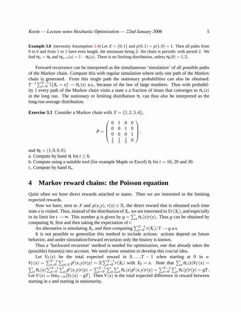
Exercise 3.1Consider a Markov chain withX = {1,2,3,4},

P =

0 1 0 00 0 1 00 0 0 113

13

13 0

,

andπ0 = (1,0,0,0).a. Compute by handπt for t ≤ 6.b. Compute using a suitable tool (for example Maple or Excel)πt for t = 10, 20 and 30.c. Compute by handπ∗.

4 Markov reward chains: the Poisson equation

Quite often we have direct rewards attached to states. Then we are interested in the limitingexpected rewards.

Now we have, next toX and p(x,y), r(x) ∈ R, the direct reward that is obtained each timestatex is visited. Thus, instead of the distribution ofXt , we are interested inEr(Xt), and especiallyin its limit for t → ∞. This numberg is given byg =

∑xπ∗(x)r(x). Thusg can be obtained by

computingπ∗ first and then taking the expectation ofr.An alternative is simulatingXt , and then computing

∑T−1t=0 r(Xt)/T→ g a.s.

It is not possible to generalize this method to include actions: actions depend on futurebehavior, and under simulation/forward recursion only the history is known.

Thus a ‘backward recursion’ method is needed for optimization, one that already takes the(possible) future(s) into account. We need some notation to develop this crucial idea.

Let VT(x) be the total expected reward in 0, . . . ,T − 1 when starting at 0 inx:VT(x) =

∑T−1t=0

∑y∈X pt(x,y)r(y) = E

∑T−1t=0 r(Xt) with X0 = x. Note that

∑xπ∗(x)VT(x) =∑

xπ∗(x)∑T−1

t=0∑

y pt(x,y)r(y) =∑T−1

t=0∑

y

∑xπ∗(x)pt(x,y)r(y) =

∑T−1t=0

∑yπ∗(y)r(y) = gT.

Let V(x) = limT→∞[VT(x)−gT]. ThenV(x) is the total expected difference in reward betweenstarting inx and starting in stationarity.


We calculateVT+1(x) in two different ways.VT+1(x) = VT(x)+∑

yπT(y)r(y) for π0 withπ0(x) = 1. As πT → π∗ and

∑xπ∗(x)r(x) = g, VT+1(x) = VT(x)+g+o(1), whereo(1) means

that this term disappears ift→ ∞. On the other hand, forVT+1 the following recursive formula-tion exists:

VT+1(x) = r(x)+∑

y

p(x,y)VT(y). (2)

ThusVT(x)+g+o(1) = r(x)+

∑y

p(x,y)VT(y).

SubtractgT from both sides, and takeT→ ∞:

V(x)+g = r(x)+∑

y

p(x,y)V(y). (3)

This equation is also known as the Poisson equation. Note thatV represents the information onthe future.

Note however that Equation (3) does not have a unique solution: IfV is a solution, then so isV ′(x) = V(x)+C. There are two possible solutions: either takeV(0) = 0 for some “reference”state 0, or add the additional condition

∑xπ∗(x)V(x) = 0. Only under the latter conditionV

has the interpretation as the total expected difference in reward between starting in a state andstarting in stationarity.

Exercise 4.1Consider the Markov chain from Exercise3.1, and taker = (0,0,0,1).a. Findg using the results obtained for Exercise3.1.b. Argue why limT→∞VT(x)/T = g.c. Compute using a suitable computer toolVT for T = 10,20,50, and 100. Compute alsoVT−gTandVT/T.d. Findg by solving the Poisson equation. Give also all solutions forV and also the one with∑

xπ∗(x)V(x) = 0.

5 Markov decision chains: policy iteration

Finally we introduce decisions. Next to the state spaceX we have an action setA . The idea isthat depending on the stateXt an actionAt is selected, according to some policyR: X →A . ThusAt = R(Xt).

Evidently the transition probabilities also depend on the action:p(x,a,y) is the probabilityof going fromx to y whena is chosen. Also the rewards depend on the actions:r(x,a).

Assumption 5.1 |A |< ∞.

We also have to adapt the assumptions we made earlier. Assumption3.2, which states that|X |< ∞, remains unchanged. For the other two assumption we have to add that they should holdfor any policyR.


Assumption 5.2 For every policy R there is at least one state x∈ X (that may depend on R),such that there is a path from any state to x. If this is the case we call the chain unichain, state xis called recurrent.

Assumption 5.3 For every policy R the gcd of all paths from x to x is 1, for some recurrent statex. If this is the case we call the chain aperiodic.

LetVRt (x) be the total expected reward in 0, . . . , t−1, when starting at 0 inx, under policyR.

We are interested in finding argmaxR limT→∞VRT (x)/T, the maximal average expected long-run

reward. This maximum is well defined because the number of different policies is equal to|X ||A |, and thus finite.

How to compute the optimal policy?1. Take someR.2. ComputegR andVR(x) for all x.3. Find abetter R′. If none exists: stop.4. R := R′ and go to step 2.

This algorithm is calledpolicy iteration. Step 2 can be done using the Poisson equation: fora fixed policyR the direct rewards arer(x,R(x)) and the transition probabilities arep(x,R(x),y).How to do step 3? Take

R′(x) = argmaxa{r(x,a)+

∑y

p(x,a,y)VR(y)}

in each state. If the maximum is attained byR for eachx then no improvement is possible.

Example 5.4 (Replacement decisions) Suppose we have a system that is subject to wear-out, for examplea car. Every year we have to pay maintenance costs, that are increasing in the age of the system. Everyyear we have the option to replace the system at the end of the year by a new one. AfterN years we areobliged to replace the system. ThusX = {1, . . . ,N}, A = {1,2}, action 1 meaning no replacement, action2 replacement. Thusp(x,1,x+1) = 1 for x < N andp(x,2,1) = p(N,1,1) = 1 for all x. The rewards aregiven byr(x,1) =−C(x) for x < N andr(x,2) = r(N,1) =−C(x)−P for all x, with P the price of a newsystem. Consider a policyRdefined byR(1) = 1 andR(x) = 2 for x > 1, thus we replace the system if itsage is two years or higher. The Poisson equations are as follows:

VR(1)+gR =−C(1)+VR(2), VR(x)+gR =−C(x)−P+VR(1) for x > 1.

We takeV(1) = 0. Then the solution isgR = −C(1)−C(2)−P2 andVR(x) =−gR−C(x)−P, x > 1. Next we

do the policy improvement step, giving

R′(x) = argmax{−C(x)+VR(x+1),−C(x)−P+VR(1)}= argmax{−gR−C(x+1),0} for x < N.

If we assume thatC is increasing, thenR′ is 1 up to somex and 2 above it.Take, for example,C(x) = x andP = 10. ThengR =−6.5 andVR(x) =−3.5−x, x > 1. From this it

follows thatR′(1) = · · · = R′(5) = 1, R′(6) = · · · = R′(N) = 2, with average rewardgR′ = (−1−2−3−4−5−6−10)/6≈−5.17>−6.5 = gR. Note that there are two optimal policies, that replace after 4 or5 years, with average cost 5.


For the optimal policyR∗ it holds that

r(x,R∗(x)))+∑

y

p(x,R∗(x),y)VR∗(y) = maxa{r(x,a)+

∑y

p(x,a,y)VR∗(y)}.

At the same time, by the Poisson equation:

VR∗(x)+gR∗ = r(x,R∗(x)))+∑

y

p(x,R∗(x),y)VR∗(y).

Combining these two gives

VR∗(x)+gR∗ = maxa{r(x,a)+

∑y

p(x,a,y)VR∗(y)}.

This equation is called theoptimality equationor Bellman equation. Often the superscript is leftout: g andV are simply the average reward and value function of the optimal policy.

Exercise 5.1Consider Example5.4, with N = 4, P = 3, C(1) = 5, C(2) = 10, C(3) = 0 andC(4) = 10. Start withR(x) = 2 for all x. Apply policy iteration to obtain the optimal policy.

6 Markov reward chains: backward recursion

In this section we go back to the Markov reward chains to obtain an alternative method forderivingV. Recall thatVT+1(x)−VT(x)→ g, and note thatVT(x)−VT(y)→V(x)−V(y). Thussimply by computingVT for T big we can obtain all values we are interested in. To computeVT

we can use the recursion (2). Initially one usually takesV0 = 0, although a good initial value canimprove the performance significantly. One stops iterating if the following holds:

span(Vt+1(x)−Vt(x))≤ ε for all x∈ X ,

which is equivalent to

there exists ag such thatg− ε2≤Vt+1(x)−Vt(x)≤ g+

ε2

for all x∈ X .

Value iteration algorithm pseudo code Let |X | = N, E(x) ⊃ {y|p(x,y) > 0}, andε somesmall number (e.g., 10−6).

Vector V[1..N], V ′[1..N]Float min, maxV← 0do {

V ′←V


for (x = 1, ..,N) { % iterateV(x)← r(x)for (y∈ E(x)) V(x)←V(x)+ p(x,y)V ′(y) }

max←−1010

min← 1010

for (x = 1, ..,N) { % compute span(V−V ′)if (V(x)−V ′(x) < min) min←V(x)−V ′(x)if (V(x)−V ′(x) > max) max←V(x)−V ′(x) } }

while(max−min> ε)

Some errors to avoid:- Avoid takingE(x) = X , but use the sparseness of the transition matrixP;- ComputeP online, instead of calculating all entries ofP first;- Insert the code for calculatingP at the spot, do not use a function or subroutine;- Span(V−V ′) need not be calculated at every iteration, but once every 10th iteration for example.

7 Markov decision chains: backward recursion

Value iteration works again in the situation of a Markov decision chain, by including actions inthe recursion of Equation (2):

Vt+1(x) = maxa{r(x,a)+

∑y

p(x,a,y)Vt(y)}. (4)

We use the same stop criterion as for the Markov reward case.

Remark 7.1 (terminology) The resulting algorithm is known under several different names. The sameholds for that part of mathematics that studies stochastic dynamic decision problems. The backward re-cursion method is best known under the name value iteration, which stresses the link with policy iteration.The field is known as Markov decision theory, although stochastic dynamic programming is also used.Note that in a deterministic setting dynamic programming can best be described by backward recursion.Thus the field is identified by its main solution method. We will call the field Markov decision theory, andwe will mainly use value iteration for the backward recursion method.

Remark 7.2 Vt(x) is interesting by itself, not just because it helps in finding the long-run average optimalpolicy: it is the maximal reward over an horizont. For studying these finite-horizon rewards we do notneed Assumptions3.3–3.4: they were only necessary to obtain limit results.

Example 7.3 Consider a graph with nodesV = {1, . . . ,N}, arc setE ⊂V ×V , and distancesd(x,y) > 0for all (x,y) ∈ E . What is the shortest path from 1 toN? This can be solved using backward recursion asfollows. TakeX = A = V . For all x < N we definer(x,a) = −d(x,a) if (x,a) ∈ E , −∞ otherwise, andp(x,a,a) = 1. Define alsor(N,a) = 0 andp(N,a,N) = 1. Start withV0 = 0. ThenVN−1 gives the minimaldistances from all points toN.

Exercise 7.1Prove the claim of Example7.3.


Exercise 7.2Consider again Example7.3.a. Formulate the Poisson equation for the general shortest path problem.b. Give an intuitive explanation whyV(N) = 0.c. Give an interpretation of the valuesV(x) for x 6= N.d. Verify this using the Poisson equation.

Exercise 7.3Consider a model withX = {0, . . . ,N}, A = {0,1}, p(x,0,x) = p(N,1,N) = λ forall x > 0, p(x,1,x+ 1) = λ for all x < N, p(0,0,0) = 1, p(0,1,0) = p(x,a,x−1) = 1− λ forall a∈ A andx > 0, r(x,0) = x− c for somec > 0, r(N,1) = N− c, andr(x,1) = x for x < N.Implement the value iteration algorithm in some suitable programming environment and reportfor different choices of the parameters (withN at least 10) on the optimal policy and values.

8 Continuous time: semi-Markov processes

Consider a Markov chain where the time that it takes to move from a statex to the next state isnot equal to 1 anymore, but some random variableT(x). This is called a semi-Markov process(Cinlar [6], Ch. 10). We assume that 0< τ(x) = ET(x) < ∞.

If we study the semi-Markov process only at the moments it changes state, the jump times,then we see what is called the embedded Markov chain. This Markov chain has stationary distri-butionπ∗. Consider now the stationary distribution over time, i.e., the time-limiting distributionthat the chain is in a certain state. This distributionν∗ is specified by:

ν∗(x)ν∗(y)

=τ(x)π∗(x)τ(y)π∗(y)

,

from which it follows that

ν∗(x) =π∗(x)τ(x)∑yπ∗(y)τ(y)

. (5)

Example 8.1 (Repair process) Take a model withX = {0,1}, p(0,1) = p(1,0) = 1, and some arbitraryT(0) andT(1). This could well model the repair of a system, withT(1) the time until failure, andT(0)the repair time. Note that the embedded Markov chain is periodic, but the stationary distribution exists:π∗(0) = π∗(1) = 1

2. Using Equation (5) we find

P(system up in long run) = ν∗(1) =π∗(1)τ(1)

π∗(0)τ(0)+π∗(1)τ(1)=

τ(1)τ(0)+ τ(1)

.

The same result can be obtained from renewal theory.

Exercise 8.1Calculateπ0, π1, π2, π∗, andν∗ for the following semi-Markov process: A machinecan be in three states: in perfect condition, deteriorated, or failed. Repair takes 5 hours, it stayson average 4 days in perfect condition, and 2 hours in a deteriorated condition. After repair thecondition is perfect, from the perfect state it breaks down completely in 60% of the cases, in 40%of the cases it continues working in the deteriorated state. It starts in perfect condition.


9 Markov processes

A special type of semi-Markov process is the one where allT(x) are exponentially distributed.Then it is called a Markov process. However, usually a Markov process is defined by itstransition ratesλ(x,y). Thus the time until the process moves fromx to y is exponentiallydistributed, unless another transition to another state occurs first. Thus, by standard proper-ties of the exponential distribution,T(x) is exponentially distributed with rate

∑yλ(x,y), and

p(x,y) = λ(x,y)/∑

zλ(x,z). Thus, Markov processes, defined through their ratesλ(x,y), areindeed special cases of semi-Markov processes.

Sometimes it is convenient to haveT(x) equally distributed for allx. Let γ be such that∑yλ(x,y) ≤ γ for all x. We construct a new process with ratesλ′(x,y) as follows. First, take

λ′(x,y) = λ(x,y) for all x 6= y. In each statex with∑

yλ(x,y) < γ, add a ‘fictituous’ or ‘dummy’transition fromx to x such that the rates sum up toγ: λ′(x,x) = γ−

∑y6=xλ(x,y) for all x∈ X .

This new process has expected transition timesτ′ as follows:τ′(x) = 1/γ. Becauseτ′(x) = τ′(y)it follows that π′∗ = ν′∗, from Equation (5). The idea of adding dummy transitions to make therates out of states constant is calleduniformization.

Using uniformization we can derive the standard balance equations for Markov processesfrom Equation (1). To do so, let us write out Equation (1), in terms of the rates. Note that for thetransition probabilities we havep′(x,y) = λ′(x,y)/γ:∑

y∈X

λ′(x,y)γ

ν′∗(x) = ν′∗(x) =∑y∈X

ν′∗(y)p′(y,x) =∑y6=x

ν′∗(y)λ′(y,x)

γ+ν′∗(x)

λ′(x,x)γ

.

Multiplying by γ, and subtractingν′∗(x)λ′(x,x) from both sides leads to∑y6=x

λ′(x,y)ν′∗(x) =∑y6=x

ν′∗(y)λ′(y,x), (6)

the standard balance equations.

Example 9.1 (M/M/1 queue) An M/M/1 queue hasX = N0, and is defined by its arrival rateλ and itsservice rateµ, thusλ(x,x+1) = λ for all x≥ 0 andλ(x,x−1) = µ for all x > 0. All other transition ratesare 0. (We assume thatλ < µ for reasons to be explained later.) Filling in the balance equations (6) leadsto

λν∗(0) = µν∗(1), (λ+µ)ν∗(x) = λν∗(x−1)+µν∗(x+1), x > 0.

It is easily verified that the solution isν∗(x) = (1− ρ)ρx, with ρ = λ/µ. Note that Assumption3.2 isviolated. Forν∗ to be a distribution we had to assume thatλ < µ.

We could have used Equation (5) right away. Note thatτ(0) = 1/λ, τ(x) = 1/(λ +µ) for x > 0, andthat p(0,1) = 1 andp(x,x−1) = µ/(λ + µ) = 1− p(x,x+ 1) for x > 0, from standard properties of theexponential distribution. This embedded chain has solution

π∗(1) =λ+µ

µπ∗(0), π∗(x) =

λ+µµ

(λµ

)x−1π∗(0) for x > 0.


This leads to

π∗(0) =µ−λ2µ

, π∗(1) =µ−λ2µ

λ+µµ

, π∗(x) =µ−λ2µ

λ+µµ

(λµ

)x−1for x > 0.

The denominator of Equation (5) is equal to 1/(2λ), leading to

ν∗(0) = 2λπ∗(0)τ(0) = 2λµ−λ2µ

1λ

= 1−ρ,

equal to what we found above. In a similar way we can findν∗(x) for x > 0.

Exercise 9.1Calculateν∗ for the following Markov processes:a. A shop can handle 2 customers at a time, and has 2 additional places for waiting. Customersthat find all places occupied do not enter and go elsewhere. Arrivals occur according to a Poissonprocess with rate 3, service times are exponential with rate 2. Take as states the number ofcustomers that are in the shop. Initially the system is empty.b. Consider a pool of 4 machines, each of which is either up or down. Time until failure isexponentially distributed with rate 1 for each machine, repair takes an exponentially distributedamount of time with rate 2. There is a single repairman, thus only one machine can be repairedat the same time. Take as states the number of machines that are up. Initially all machines arefunctioning.c. A shop can handle 1 customer at a time, and has 3 additional places for waiting. Customersthat find all places occupied do not enter and go elsewhere. Arrivals occur according to a Poissonprocess with rate 4, service times are exponential with rate 3. Waiting customers leave the shopunserved, each at a rate 1. Take as states the number of customers that are in the shop. Initiallythe system is empty.

Exercise 9.2Consider the M/M/s/s queue, which is ans-server system with arrival rateλ andservice rateµ, but without waiting places. It is also known as the Erlang B or Erlang blockingmodel.a. What is a suitable uniformization parameter?Formulate Equation (6) for this model.b. Find its solution.

10 Generalized semi-Markov processes

Sometimes a semi-Markov process is not general enough. Think of discrete-event simulation:multiple events are active at the same time, and the one that ‘fires’ first generates a change instate. The mathematical framework for this are generalized semi-Markov processes. They makea distinction between states and events, and multiple events can be active at any time. The mainsolution method of generalized semi-Markov processes is simulation (“We think of a gsMp asa model of discrete-event simulation”, Whitt ’80); for this reason we will not go into detail andpresent only the G/G/s queue as an example.


Example 10.1 (G/G/s queue) Next to the state spaceX = N0 we have a set of eventsE = {0, . . . ,s} ofwhich event 0 (the arrival process) is always active, and min{s,x} of the remainingsevents are active (thedepartures). For each of the active events there is a time when they will expire. When the first expires thestate changes and new events might become active. E.g., when an arrival occurs (event 0) whenx < s thenevent 0 is rescheduled, but also eventx+1 becomes active.

Remark 10.2 A semi-Markov process is a generalized semi-Markov process where only one event can beactive at the same time. Also Markov processes are special cases of generalized semi-Markov processes:due to the exponentiality of the event times however they can be reformulated as semi-Markov processesallowing a treatment using backward recursion.

11 Semi-Markov reward processes: Poisson equation

As for the Markov reward processes we now add rewards to the process. In the continuous-timesetting we have to decide how rewards are obtained: all at once at jump times or continuouslyover time. We choose the latter, in the section on modeling issues we discuss how one form ofrewards can be translated into the other. Thus every time unit that the process remains in statexa rewardr(x) is obtained.

We are again interested in the expected long-run stationary rewards, which is equivalent tothe long-run average or long-run expected rewards:

g = limt→∞

Er(Xt) = limt→∞

1tE∫ t

0r(Xs)ds=

∑x

ν∗(x)r(x).

Example 11.1 Take the repair process studied earlier, suppose a rewardR for each unit of time the systemis up and labour costsC for each unit of time the system is in repair. Then the expected long-run stationaryreward is given by

g =−τ(0)C+ τ(1)R

τ(0)+ τ(1).

A simple algorithm to computeg would consists of computing the stationary distribution ofthe embedded chainπ∗ and from thatν∗ and finallyg can be computed. Note thatg can also becomputed directly fromπ∗:

g =∑

x

ν∗(x)r(x) =∑

xπ∗(x)τ(x)r(x)∑yπ∗(y)τ(y)

. (7)

The denominator ofg has the following interpretation: it is the expected time between two jumpsof the process.

An alternative method is to simulate the embedded chainXt , and then to compute∑Tt=0 r(Xt)τ(Xt)∑T

t=0 τ(Xt)→ g a.s.

As for the discrete-time case, we move next to backward recursion. LetVt(x) be the totalexpected reward in[0, t] when starting at 0 inx. We are again interested in limt→∞

Vt(x)t , the

average expected long-run rewards.


Using similar arguments as for the discrete-time case we find

VT(x)+ τ(x)g+o(1) = r(x)τ(x)+∑

y

p(x,y)VT(y).

SubtractinggT from both sides and takingT→ ∞ leads to:

V(x)+ τ(x)g = r(x)τ(x)+∑

y

p(x,y)V(y) (8)

Note that again this equation does not have a unique solution.

Example 11.2 (Repair process) Consider again the repair process. We get the following set of equations:

V(0)+ τ(0)g =−Cτ(0)+V(1), V(1)+ τ(1)g = Rτ(1)+V(0)

All solutions are given by:

g =−Cτ(0)+Rτ(1)

τ(0)+ τ(1),

V(1) = V(0)+τ(0)τ(1)(R+C)

τ(0)+ τ(1)

Exercise 11.1We add a reward component to the semi-Markov process that we studied for someof the models of Exercises8.1and9.1. Compute the expected stationary reward using two differ-ent methods: by utilizing the stationary distributionν∗, and by solving the optimality equation.Give also expressions forV. The direct rewards are as follows:a. Consider Exercise8.1: There is a rewardR for each time unit the machine is up. The costs forrepairing are equal toC per unit of time.b. Consider Exercise9.1b: There is a rewardR for each time unit that a machine is up. Everyrepair costsC per unit of time for labor costs.

12 Semi-Markov decision processes: policy improvement

Finally we consider semi-Markov decision processes. Now the transition timesT(x,a) dependalso on the action that is taken at the beginning of the period after which the transition takesplace. We defineτ(x,a) = ET(x,a), and continuous rewardsr(x,a), when actiona ∈ A waschosen when reachingx∈ X and while we’re still inx.

Let VRt (x) be the total expected reward in[0, t], when starting at 0 inx, under policyR. We

are again interested in argmaxR limt→∞VR

t (x)t , the maximal average expected long-run rewards.

Policy iteration can again be used, where Equation (8) is used to evaluate a policy and the policyimprovement step consists of taking

R′(x) = argmaxa{(r(x,a)−gR)τ(x,a)+

∑y

p(x,a,y)VR(y)}.


Exercise 12.1Consider again Exercise8.1. As in Exercise11.1, there is a rewardR for eachtime unit the machine is up. The costs for repairing are equal toC per unit of time. Supposethere is the option to repair in 3 hours for costsC′ per unit of time.a. Formulate this as a semi-Markov decision process.b. Use policy iteration to determine the minimal value ofC′ for which it would be attractive tochoose the short repair times.

13 Semi-Markov reward processes: backward recursion

To derive the backward recursion algorithm for semi-Markov reward processes we note first thatthe optimal policy depends only onT(x) throughτ(x): the distribution ofT(x) does not playa role. This means that we can chooseT(x) the way we like: with 0< τ ≤ τ(x) for all x, wetakeT(x) = τG(x), whereG(x) has a geometric distribution with parameterq(x) = τ/τ(x). Thismeans thatP(G(x) = 1) = qx, P(G(x) = 2) = (1− q(x))q(x), etc. Then

∑k kP(G(x) = k) =∑

k kq(x)(1−q(x))k−1 = q(x)−1, and thus indeedET(x) = τEG(x) = τ(x).Note thatG(x) is memoryless: after each interval of lengthτ the sojourn time in statex

finishes with probabilityq(x). Thus the original system is equivalent to one with sojourn timesequal toτ and dummy transitions with probability 1−q(x). This leads to the following backwardrecursion:

V(t+1)τ(x) = r(x)τ+q(x)∑

y

p(x,y)Vtτ(y)+(1−q(x))Vtτ(x).

FromV(t+1)τ(x) = Vtτ(x)+ τg+o(1) it follows thatV(t+1)τ(x)−Vtτ(x)→ τg. Thus the valueiteration algorithm consists of takingV0 = 0, and then computingVτ,V2τ, . . .. The stop criterionis equivalent to the one for the discrete-time case.

14 Semi-Markov decision processes: backward recursion

Value iteration can again be generalized to the case that includes decisions. This leads to thefollowing value function:

V(t+1)τ(x) = maxa{r(x,a)τ+q(x,a)

∑y

p(x,a,y)Vtτ(y)+(1−q(x,a))Vtτ(x)}.

The last policy is optimal, and[V(t+1)τ(x)−Vtτ(x)]/τ for t sufficiently large gives the maximalaverage rewards.

Remark 14.1 In the discrete-time settingVt(x) had an interpretation: it is the total expected maximalreward int time units. In the continuous-time caseVtτ(x) does not have a similar interpretation, due to therandomness ofT(x,a).

Exercise 14.1Consider the repair process of Example11.2. Takeτ(1) = 5, τ(0) = 2, R= 2 andC = 0. Here there is also the additional option to shorten repair times to 1, for costs 1.


a. Formulate the value function.b. Solve it using a suitable computer program of package.c. Find the optimal policy as a function of the parametert. Can you explain what you found?

15 Other criterion: discounted rewards

Average rewards are often used, but sometimes there are good reasons to give a lower value to areward obtained in the future than the same reward right now.

Example 15.1 A reward of 1 currently incurred will be 1+β after one year if put on a bank account withan interest rate ofβ. Thus a reward of 1 after 1 year values less than a reward of 1 right now.

In the example we considered a yearly payment of interest of rateβ. To make the step tocontinuous-time models, we assume that each year is divided inmperiods, and after each periodwe received an interest ofβ/m. Thus aftert years our initial amount 1 has grown to(1+ β

m)tm.This converges toeβt asm→ ∞. Thus, in a continuous-time model with interestβ, an amount of1 valueseβt after t years. By dividing byeβt we also obtain: Reward 1 at 1 is evaluated at 0 ase−β. This generalizes to reward 1 att is evaluated at 0 ase−βt .

Because∫ ∞

0 e−βtdt < ∞ the total expected discounted rewards are well defined. LetVβ(x) bethe total expected discounted rewards, starting inx. Note that the starting state is crucial here,unlike for the average reward model.

To determineVβ(x), we first have to derive the total expected discounted rate rewards if themodel is inx from 0 toT(x). If r(x) = 1, then this is equal to

E∫ T(x)

0e−βsds.

We write E f (T(x)) =∫ ∞

0 f (t)dT(x)(t), irrespective of the type of distribution ofT(x). (Thisnotation comes from measure theory.) Then

E∫ T(x)

0e−βsds=

∫ ∞

0

∫ t

0e−βsdsdT(x)(t) = β−1(1− γ(x)),

with γ(x) = Ee−βT(x), the so-calledLaplace-Stieltjes transformof T(x) in β. FromT(x) on thediscounted rewards are equal toVβ(y) with probability p(x,y), but discounted withEe−βT(x) =γ(x). Thus the Poisson equation (8) has the following discounted equivalent:

Vβ(x) = β−1(1− γ(x))r(x)+ γ(x)∑

y

p(x,y)Vβ(y).

This can of course be utilized as part of a policy improvement algorithm. The improvement stepis then given by:

R′(x) = argmaxa{β−1(1− γ(x,a))r(x,a)+ γ(x,a)

∑y

p(x,a,y)VRβ (y)}.


The optimality equation becomes

Vβ(x) = maxa{β−1(1− γ(x,a))r(x,a)+ γ(x,a)

∑y

p(x,a,y)Vβ(y)},

and also value iteration works for the discounted model.

Remark 15.2 It is interesting to note that discounting is equivalent to taking total rewards up toT withT random and exponential. Indeed, letr(t) be a function indicating the rate reward att. Let T ∼ exp(β).Thenc(t)e−βt is the expected reward att, equal to the discounted reward.

Exercise 15.1Determine the Laplace-Stieltjes tranforms of the exponential and gamma distri-butions.

Exercise 15.2Repeat exercise12.1for the discounted reward case. Consider the cases in whichthe transition times are constant and exponentially distributed, for some well-chosenβ.

Exercise 15.3Consider a Markov reward process with state spaceX = {0,1}, p(0,1) =p(1,0) = 1, T0 is exponentially distributed,T1 is constant, andr = (1,0). Assume that thereward att is discounted with a factore−βt for someβ > 0. LetVβ(x) be the long-run expecteddiscounted reward for initial statex.a. Give a set of equations forVβ and solve it.b. Compute limβ→0βVβ.c. Give an interpretation for the results you found for b.

16 (Semi-)Markov decision processes: literature

Some literature on the theory of (semi-)Markov decision chains/processes: Bertsekas [3], Kallen-berg [10], Puterman [13], Ross [14], Tijms [16].

17 Modeling issues

Suppose you have some system or model that requires dynamic optimization. Can it be(re)formulated as a (semi-)Markov decision problem, and if so, how to do this in the best way?Different aspects of this question will be answered under the heading ‘modeling issues’.

Modeling issues: dependence on next state

Let us start by introducing some simple generalizations to the models that can sometimes bequite helpful.

Sometimes it is more appropriate to work with costs instead or rewards. This is completelyequivalent, by multiplying all rewards with−1 and replacing max by min everywhere.


It sometimes occurs that the direct rewardsr ′ depend also on the next state:r ′(Xt ,At ,Xt+1).We are interested in the sum of the expected rewards,E

∑T−1t=0 r ′(Xt ,At ,Xt+1), which gives

ET−1∑t=0

r ′(Xt ,At ,Xt+1) =T−1∑t=0

Er ′(Xt ,At ,Xt+1) = ET−1∑t=0

∑y∈X

p(Xt ,At ,y)r ′(Xt ,At ,y).

Thus we can replace the direct rewardsr ′(x,a,y) by r(x,a) =∑

y p(x,a,y)r ′(x,a,y), which fitswithin our framework.

A similar reasoning can be applied to the case where the transitions times dependalso on y, notation T ′(x,a,y) with τ′(x,a,y) = ET ′(x,a,y). In this case, takeτ(x,a) =∑

y p(x,a,y)τ′(x,a,y).

Modeling issues: lump rewards

We presented the theory for continuous-time models assuming that rewards are obtained in acontinuous fashion, so-called rate rewards. Sometimes rewards are obtained in a discrete fashion,once you enter or leave a state (and after having chosen an action):lump rewards. In the long runlump rewardsr l (x,a) are equivalent to rewardsr l (x,a)/τ(x,a). If we write out Equation (7) forlump rewards instead of rate rewards, then we get the following somewhat simpler expression:

g =∑

xπ∗(x)r l (x)∑yπ∗(y)τ(y)

.

Note that now also the numerator has a simple interpretation: it is the expected lump reward perjump of the process.

Modeling issues: aperiodicity

Forward and backward recursion do not need to converge in the case of Markov (decision) chainsthat are periodic. This we illustrate with an example.

Example 17.1 Consider a Markov reward chain withX = {0,1}, r = (1,0), p(0,1) = p(1,0) = 1. Thischain is periodic with period 2. If we apply value iteration, then we get:

Vn+1(0) = 1+Vn(1), Vn+1(1) = 1+Vn(0).

TakeV0(0) = V0(1) = 0. Then

Vn(0) ={ n

2 if n even;n+1

2 if n odd, Vn(1) ={ n

2 if n even;n−1

2 if n odd.

From this it follows that

Vn+1(0)−Vn(0) ={

1 if n even;0 if n odd,

Vn+1(1)−Vn(1) ={

0 if n even;1 if n odd.

But in this case the stop criterion is never met: span(Vn+1−Vn) = 1 for all n.


A simple trick to avoid this problem is to introduce a so-calledaperiodicity transformation.It consists in fact of adding a dummy transition to each state, by replacingP by δP+(1− δ)I ,0 < δ < 1. Thus with probability 1− δ the process stays in the current state, irrespective of thestate and action; with probabilityδ the transition occurs according to the original transition prob-abilities (which could also mean a transition to the current state). Because it is now possible tostay in every state, the current chain is aperiodic, and forward and backward recursion converge.This model has the following Poisson equation:

V +g = r +(δP+(1−δ)I)V = r +PδV +(1−δ)V⇔ δV +g = r +PδV. (9)

If (V,g) is a solution ofV + g = r + PV, then (V/δ,g) is a solution of Equation (9). Thusthe average rewards remain the same, andV is multiplied by a constant. This is intuitivelyclear, because introducing the aperiodicity transformation can be interpreted as slowing downthe system, making it longer for the process to reach stationarity.

Modeling issues: states

The first and perhaps most important choice when modeling is how to choose the states of themodel. When the states are chosen in the wrong way, then sometimes the model cannot be putinto our framework. This fact is related to the Markov property, which we discuss next.

Definition 17.2 (Markov property) A Markov decision chain has the Markov property ifP(Xt+1 = x|Xt = xt ,At = at) = P(Xt+1 = x|Xs = as,As = as, s= 1, . . . , t) for all t, x, and xs,as

for s= 1, . . . , t.

Thus the Markov property implicates that the history does not matter for the evolution of theprocess, only the current state does. It also shows us how to take the transition probabilitiesp:p(x,a,y) = P(Xt+1 = y|Xt = x,At = at), where we made the additional assumption thatXt+1|Xt ,At

does not depend ont, i.e., the system is time-homogeneous. If the Markov property does not holdfor a certain sytem then there are no transition probabilities that describe the transition law, andtherefore this system cannot be modeled as a Markov decision chain (with the given choice ofstates). For semi-Markov models we assume the Markov property for the embedded chain. Notethat for Markov (decision) processes the Markov property holds at all times, because of thememoryless property of the exponentially distributed transition times.

It is important to note that whether the Markov property holds might depend on the choice ofthe state space. Thus the state space should be chosen such that the Markov property holds.

Example 17.3 Consider some single-server queueing system for which we are interested in the numberof customers waiting. If we take as state the number of customers in the queue, then information onprevious states gives information on the state of the server which influences the transitions of the queue.Therefore the Markov property does not hold. Instead, one should take as state the number of customersin the system. Under suitable conditions on service and interarrival times the Markov property holds. Thequeue length can be derived from the number of customers in the system.


Our conclusion is that the state space should be chosen such that the Markov property holds.Next to that, note that policies are functions of the states. Thus, for a policy to be implementable,the state should be observable by the decision maker.

Remark 17.4 A choice of state space satisfying the Markov property that always works is taking allprevious observations as state, that is, the observed history is the state. Disadvantages are the growing sizeof the state space, and the complexity of the policies.

Modeling issues: decision epochs

Strongly related to the choice of states is the choice of decision epoch. Several choices arepossible: does the embedded point represent the state before or after the transition or decision?This choice often has consequences for the states.

Example 17.5 Consider a service center to which multiple types of customers can arrive and where de-cisions are made on the basis of the arrival. If the state represents the state after the arrival but before thedecision, then the type of arrival should be part of the state space. On the other hand, if the state representsthe state before the potential arrival then the type of arrival will not be part of the state; the actions howeverwill be more-dimensional, with for each possible arrival an entry.

The general rule when choosing the state space and the decision epochs is to do it such thatthe size of the state space is minimized. To make this clear, consider the following examplesfrom queueing theory.

The M/M/1 queue can be modeled as a Markov process with as decision epochs all events(arrivals and departures) in the system, and as states the number of customers. In the case of theM/G/1 queue this is impossible: the remaining service time depends not only on the number ofcustomers in the system, and thus the Markov property does not hold. There are two solutions:extend the state space to include the attained or remaining service time (the supplementary vari-able approach) or choose the decision epoch in such a way that the state space remains simple.We discuss methods to support both approaches, the latter first.

Example 17.6 Consider a model withs servers that each work with rateµ, two types of customers thatarrive with ratesλ1 andλ2, no queueing, and the option to admit an arriving customer. Blocking costsci for type i, if all servers are busy the only option is blocking. How to minimize blocking costs? Whenmodeling this as a Markov decision process we have to choose the states and decision epochs. The problemhere is that the optimal action depends on the type of event (e.g., an arrival of type 1) that is happening.There are two solutions to this: either we take state space{0, . . . ,s}×{a1,a2,d}, the second dimensionindicating the type of event. This can be seen as epoch the state after the transition but before a possibleassignment. We can also take as state space{0, . . . ,s}, but then we have as action{0,1}×{0,1} with theinterpretation that action(a1,a2) means that if an arrival of typei occurs then actionai is selected. Thishas the advantage of a smaller state space and is preferable.

Exercise 17.1Give the transition probabilities and direct rewards for both choices of decisionepochs of Example17.6.


Modeling issues: Poisson arrivals in interval of random length

Consider again the M/G/1 queue. To keep the state space restricted to the number of customersin the system the decision epochs should lie at the beginning and end of the service times, whichhave a durationS. This means thatτ(x) = ESfor x> 0. We takeτ(0) = 1/λ, and thusp(0,1) = 1,p(x,x−1+k) = P(k arrivals inS) for x> 0. Let us consider how to calculate these probabilities.First note that

qk = P(k arrivals inS) =∫ ∞

0

(λt)k

k!e−λtdS(t).

Let us calculate the generating functionQ of theqks:

Q(α) :=∞∑

k=0

qkαk =∫ ∞

0e−λt(1−α)dS(t) = g(λ(1−α)),

with g thus the Laplace-Stieltjes transform ofS. The coefficientsqk can be obtained fromQ inthe following way:Q(k)(0) = (−λ)kg(k)(λ) = qkk!. In certain cases we can obtain closed-formexpressions for this.

Example 17.7 (Sexponential) SupposeS∼ Exp(µ), theng(x) = 11+x/µ. From this it follows thatQ(α) =

(1+λ(1−α)/µ)−1, and thus

Q(n)(0) = n!(λµ)n(1+λ/µ)−(n+1) = n!(

λλ+µ

)n µλ+µ

.

From this it follows thatqk = ( λλ+µ)k µ

λ+µ, and thus the number of arrivals is geometrically distributed.

If there is no closed-form expression for theqk then some numerical approximation has to beused.

Modeling issues: Phase-type distributions

As said when discussing the choice of decision epochs, another option to deal with for examplethe M/G/1 queue is adding an additional state variable indicating the attained service time. Thisnot only adds an additional dimension to the state space, but this extra dimension describes acontinuous-time variable. This can be of use for theoretical purposes, but from an algorithmicpoint of view this variable has to be discretized in some way. A method to do so with a clearinterpretation is the use ofphase-type distributions.

The class of phase-types distributions can be defined as follows.

Definition 17.8 (Phase-type distributions) Consider a Markov process with a single absorbingstate 0 and some initial distribution. The time until absorbtion into 0 is called to have a Phase-type (PH) distribution.


Example 17.9 The exponential, gamma (also called Erlang or Laplace), and hyperexponential distribu-tions (the latter is a mixture of 2 exponential distributions) are examples of PH distributions.

An interested property of PH distributions is the fact that the set of all PH distributions isclosed in the set of all non-negative distributions, i.e., any distribution can be approximatedarbitrarily close by a PH distribution. This holds already for a special class of PH distributions,namely for mixtures of gamma distributions (all with the same rate).

Consider some arbitrary distribution functionF , and writeE(k,m) for the distribution func-tion of the gamma distribution withk phases (the shape parameter) and ratem.

Theorem 17.10For m∈N, takeβm(k) = F( km)−F(k−1

m ) andβm(m2) = 1−F(m2−1m ). Then for

Fm with Fm(x) =∑m2

k=1βk(m)E(k,m)(x) it holds thatlimm→∞ Fm(x) = F(x) for all x≥ 0.

Proof The intuition behind the result is thatE(km,m)(x)→ I{k≤ x} and that∑m2

k=1 βk(m)I{k/m≤ x}→F(x). An easy formal proof is showing that the Laplace-Stieltjes transforms ofFm converge to the trans-form of F (which is equivalent to convergence in distribution).

Modeling issues: Little’s law and PASTA

Sometimes we are interested in maximizing performance measures that cannot be formulateddirectly as long-run average direct rewards, e.g., minimizing the average waiting time in somequeueing system. There are two results that are helpful in translating performance measures suchthat they can be obtained through immediate rewards: Little’s law and PASTA.

Little’s law is an example of acost equation, in which performance at the customer levelis related to performance at the system level. E.g., in a system with Poisson arrivals it gener-ally holds thatEL = λEW with L the stationary queue length,W the stationary waiting time ofcustomers, andλ the arrival rate. See El-Taha & Stidham [8] for an extensive treatment of costequations.

PASTA stands for ‘Poisson arrivals see time averages’. It means that an arbitrary arrival seesthe system in stationarity. For general arrival processes this is not the case.

Example 17.11 (Waiting times in the M/M/1 queue) Suppose we want to calculate the waiting time inthe M/M/1 queue by backward recursion. Denote the waiting time byWq, and the queue length byLq.Then Little’s law states thatEWq = ELq/λ. If the statex denotes the number in the system, then takingimmediate rewardr(x) = (x−1)+/λ will give g = EWq.

We can calculateEWq also using PASTA. PASTA tells us thatEWq = EL/µ: we have to wait for allthe customers to leave, including the one in service. Thus takingr(x) = x/µ also givesg = EWq.

The equivalence of both expressions forEWq can be verified directly from results for the M/M/1queue, usingEL = ρ/(1−ρ) andEL = ELq +ρ with ρ = λ/µ:

ELQ

λ=

EL−ρλ

=ρ

1−ρ

λ− 1

µ=

1µ−λ

− 1µ

=λ

µ(µ−λ)=

ELµ

.


Modeling issues: Countable state spaces

In our physical world all systems are finite, but there are several reasons why we would be inter-ested in systems with an infinite state space: infinite systems behave ‘nicer’ than finite systems,bounds cannot exactly be given, the state space does not represent something physical but someconcept of an unbounded nature, and so forth.

Example 17.12 (M/M/1 vs. M/M/1/N queue) For the M/M/1 queue there are nice expressions for themost popular performance measures, for the M/M/1/N queue these expressions are less attractive.

Example 17.13 (Work in process in production systems) In certain production systems the amount ofwork of process that can be stocked is evidently bounded. In other production systems such as adminis-trative processes this is less clear: how many files that are waiting for further processing can a computersystem store? This question is hard to answer if not irrelevant, given the current price of computer diskspace.

Example 17.14 (Unobserved repairable system) Suppose we have some system for which we have noimmediate information whether it is up or not, but at random times we get a signal when it is up. A naturalcandidate for the states are the numbers of time units ago since we last got a signal. By its nature this isunbounded.

Although we have good reasons to prefer in certain cases infinite state spaces, we need afinite state space as soon as we want to compute performance measures or optimal policies. Apossible approach is as follows.

Consider a model with countable state spaceX . Approximate it by a series of models with fi-nite state spacesX n, such thatX n+1⊃ X n and limn→∞ X n = X . Let thenth model have transitionprobabilitiesp(n). These should be changed with respect top such that there are no transitionsfrom X n to X \X n. This can for example be done by taking for eachx∈ X n

p(n)(x,y) = p(x,y) for x 6= y∈ X n, p(n)(x,y) = 0 for y 6∈ X n, p(n)(x,x) = p(x,x)+∑y6∈X n

p(x,y).

Having defined the approximating model it should be such that the performance measure(s) ofinterest converge to the one(s) of the original model. There is relatively little theory about thesetypes of results, in practice one compares for exampleg(n) andg(n+1) for different values ofn.

Example 17.15 (M/M/1 queue) As finitenth approximation for the M/M/1 queue we could take theM/M/1/n queue. If and only if the queue is stable (i.e.,λ < µ) thenν(n)

∗ (x)→ ν∗(x) for all x.

Exercise 17.2Consider theM|D|1 queue with a controllable server: at the beginning of a servicetime we may decide whether the service time isd1 or d2 (d1 < d2). There are additional costs formaking the server work hard. Next to that there are costs for every unit of time that a customerspends waiting. The objective is to minimize the long-run average costs.a. Give the value iteration formula (i.e., give an expression forV(n+1)τ in terms ofVnτ), specifyingthe values forp, r, τ, etc.


b. Make the state space finite by choosing some suitable bound and formulate again the valueiteration formula.c. Implement the value iteration algorithm in some suitable programming environment and reportfor different choices of the parameters on the optimal policy and values. Pay special attentionto the question whether the bound approaches the unbounded system well enough, and take theimplementation remarks from the end of Section6 into account.

Exercise 17.3Consider theD|M|1 queue. Every finished customer gives a rewardr, by givinga discountd when entering we can decrease the interarrival time froma1 to a2. There are costsfor every unit of time that a customer spends waiting. The objective is to minimize the long-runaverage costs. Answer the same questions as in Exercise17.2for this model.

18 Curse of dimensionality

We see in practice that Markov decision chains are less used than we might expect. The reasonfor this is thecurse of dimensionality, as already described in 1961 in Bellman [2]. A fact is thatmost practical problems have multi-dimensional state spaces. Now suppose we have a modelwith state spaceX = {(x1, . . . ,xn)|xi = 1, . . . ,B}. Then the number of different states is|X |= nB.Note from the backward recursion algorithm that we need in memory at least one double forevery state, thus the memory use is at least|X | floating point numbers. Forn = B = 10 thiswould require±100 Gb of memory, without even thinking about the processing requirementsthat would be necessary.

Example 18.1 (Production process) Consider a production process forN products, where productn hasKn production steps (on in totalM machines), and production stepk for productn hasBnk buffer spacesfor waiting jobs. A typical decision is which job to schedule next on each machine. The number ofdimensions is (at least)

∑Nn=1Kn, with

∏Nn=1

∏Knk=1(Bnk+1) the number of states. This would be sufficient

if all machines had a production time of 1 and no costs for switching from one product to the next. If thisis the case (as it is often in job shops) then additional state variables indicating the states of the machineshave to be added.

Example 18.2 (Service center) Consider a service center (such as a call center) where customers of dif-ferent types arrive, with multiple servers that can each process a different subset of all customer types.To model this we need at least a variable for each customer class and a variable for each server (class).Service centers with 5 or 10 customer and server classes are no exception, leading to 10 or 20 dimensions.

In the following sections we will discuss a number of approximation methods that can beused (in certain cases) to solve high-dimensional problems.

Exercise 18.1Consider a factory withmmachines andn different types of products. Each prod-uct has to be processed on each machine once, and each type of product has different processingrequirements. There is a central place for work-in-process inventory that can hold a total ofkitems, including the products that are currently in service. Management wants to find optimal


dynamic decisions concerning which item to process when on which machine. Suppose one con-siders to use backward recursion.a. What is the dimension of the state space?b. Give a description of the state space.c. Give a formula for the number of states.d. Give a rough estimate of this number form= n = k = 10.

19 One-step improvement

The one-step improvement works only for models for which the value function of a certain fixedpolicy R can be obtained, without being hindered by the curse of dimensionality. Crucial is thefact that practice shows that policy improvement gives the biggest improvement during the firststeps. One-step improvement consist of doing the policy improvement step on the basis of thevalue ofR. It is guaranteed to give a better policyR′, but how goodR′ is cannot be obtained ingeneral, because of the curse of dimensionality.

Note that it is almost equally demanding to store a policy in memory than it is to store a valuefunction in memory. For this reason it is often better to compute the action online. That is, if thecurrent state isx, thenVR(y) is calculated for eachy for which p(x,a,y) > 0 for somea, and onthe basis of these numbersR′(x) is computed. Note that the sparseness of the matrixP is crucialin keeping the computation time low.

The most challenging step in one-step improvement is computingVR for some policyR. Thepractically most important case is whereR is such that the Markov process splits up in severalindependent processes. We show how to findVR on the basis of the value functions of thecomponents.

Suppose we haven Markov reward processes with statesxi ∈ X i , rewardsr i , transition ratesλi(xi ,yi), uniformization parametersγi , average rewardsgi , and value functionsV i . Consider nowa model with statesx = (x1, . . . ,xn) ∈ X = X 1×·· ·×X n, rewardsr(x) =

∑ni=1 r i(xi), transition

ratesλ(x,y) = λi(xi ,yi) if x j = y j for all j 6= i, average rewardg, and value functionV.

Theorem 19.1 g =∑

i gi and V(x) =

∑i V

i(xi) for all x ∈ X .

Proof Consider the Poisson equation of componenti:

V i(xi)∑

yi

λi(xi ,yi)+gi = r i(xi)+∑

yi

λi(xi ,yi)V i(yi).

Sum overi and add∑

yi λi(xi ,yi)∑

j 6=i Vj(x j) to both sides. Then we get the optimality equation of the

system as specified, withg =∑

i gi andV =

∑i V

i .

Example 19.2 Consider a fully connected communication network, where nodes are regional switchesand links consists of several parallel communication lines. The question to be answered in this networkis how to route if all direct links are occupied? To this model we apply one-step optimization with initialpolicy R that rejects calls if all direct links are occupied. This implies that all link groups are independent,


and Theorem19.1can be used to calculate the value function for each link group. If a call arrives for acertain connection and all direct links are occupied, then online it is calculated if and how this call shouldbe redirected. Note that in this case it will at least occupy two links, thus it might be optimal to reject thecall, even if routing over multiple links is possible.

Calculating the value for each link group can be done very rapidly, because these are one-dimensionalproblems. But they even allow for an exact analysis, if we assume that they behave like Erlang lossmodels.

We derive the value function of an Erlang loss model with parametersλ, µ= 1, s, and “reward” 1 perlost call. The Poisson equation is as follows:

sV(s)+g = λ+sV(s−1);

x < s : (x+λ)V(x)+g = λV(x+1)+xV(x−1).

Note that we are only interested in differences of value functions, not in the actual values. These differ-ences andg are given byg = λB(s,a) andV(k+1)−V(k) = B(s,a)/B(k,a) with a = λ/µ and

B(k,a) =ak/k!∑kj=0a j/ j!

,

the Erlang blocking formula. This example comes from Ott & Krishnan [12].

Example 19.3 (value function M/M/1 queue) The M/M/1 queue with the queue length as immediatereward is another example for which we can compute the value function explicitly. Instead of solvingthe Poisson equation we give a heuristic argument. It is known thatg = λ/(µ−λ). By using a couplingargument it is readily seen thatV(x+1)−V(x) = (x+1)EB, with B the length of a busy period. ForEBwe can obtain the following relation by conditioning on the first event in a busy period:

EB =1

λ+µ+

λλ+µ

2EB⇒ EB = (µ−λ)−1,

and thus

V(x)−V(0) =x∑

i=1

(V(i)−V(i−1)) =x(x+1)2(µ−λ)

.

Exercise 19.1Consider anM/M/s/s queue with two types of customers, arrival ratesλ1, λ2,andµ1 = µ2. Blocking costs are different, we are interested in the average weighted long-runblocking costs. Giveg andV for this queue. Now we have the possibility to block customers,even if there are servers free. What will be the form of the policy after one step of policy iteration?Compute it for some non-trivial parameter values.

Exercise 19.2We consider a single arrival stream with rate 2 that can be routed to two parallelsingle-server queues, with service rates 1 and 2. Consider first a routing policy that assigns allcustomers according to i.i.d. Bernoulli experiments, so-called Bernoulli routing. We are inter-ested in the average total long-run number of customers in the system. Compute the optimalrouting probability and theg andV belonging to this policy. Show how to compute the one-stepimproved policy. How can you characterize this policy?


20 Approximate dynamic programming

Approximate dynamic programming is another, more ambitious method to solve high-dimensional problems. It was introduced in the dynamic programming community and furtherformalized in Bertsekas & Tsitsiklis [4].

The central idea is thatVR(x) can be written as or estimated by a function with a knownstructure (e.g., quadratic in the components). Let us call this approximationWR(r,x), with r thevector of parameters of this function. Thus the problem of computingVR(x) for all x is replacedby computing the vectorr, which has in general much less entries.

Example 20.1 Let WR(r,x) represent the value function for the long-run average weighted queue lengthin a single-server 2-class preemptive priority queue with Poisson arrivals and exponential service times.ThenWR(r,x) = r0 + r1x1 + r2x2 + r11x2

1 + r22x22 + r12x1x2, with xi the number of customers of typei in

the system. Instead of computingVR(x) for all possiblex we only have to determine the six coefficients.(Groenevelt et al. [9])

A summary of the method is as follows (compare with policy iteration):0. Choose some policyR.1. Simulate/observe model to estimateVR by VR in statesx∈ X ′ ⊂ X ;2. ApproximateVR(x) by WR(r,x) (with r such that it minimizes

∑x∈X ′ |VR(x)−WR(r,x)|);

3. Compute new policyR′ minimizingWR(r,x), go to step 1 withR= R′.

21 LP approach

For Markov reward chains we saw in Section4 that the average rewardg is equal to∑x

π∗(x)r(x)

with π∗ the unique solution of ∑y

π∗(y)p(y,x)−π∗(x) = 0

and ∑x

π∗(x) = 1, π∗(x)≥ 0.

Of course,π∗ can be seen as the stationary distribution.The same approach applies to Markov decision chains: the maximal average reward is given

bymax

∑x

∑a

π∗(x,a)r(x,a)

subject to ∑y

∑a

π∗(y,a)p(y,a,x)−∑

a

π∗(x,a) = 0


and ∑x

∑a

π∗(x,a) = 1, π∗(x,a)≥ 0.

Now theπ∗(x,a) are called the (stationary) state-action frequencies, they indicate which frac-tion of the time the state isx and actiona is chosen at the same time,

∑aπ∗(x,a) can be inter-

preted as the stationary probability of statex under the optimal policyR∗. For recurrent statesπ∗(x,a) > 0 for at least onea∈ A , but there might be more. Any actiona for whichπ∗(x,a) > 0is optimal inx. However, the standard simplex method will find only solutions withπ∗(x,a) > 0for onea per x. To see this, consider the number of equations. This isX + 1. However, oneinequation is redundant, because the firstX rows are dependent:∑

x

[∑

y

∑a

π∗(y,a)p(y,a,x)−∑

a

π∗(x,a)] = 0.

Thus we can leave out one of the inequalities, giving a total ofX . Now the simplex methodrewrites the constraint matrix such that each solution it evaluates consists of a number of non-negativebasicvariables (equal to the number of constraints) and a number ofnon-basicvariablesequal to 0. In our case there are thusX basic variables, one corresponding to each state.

Exercise 21.1Give the LP formulation for semi-Markov decison processes.

22 Multiple objectives

Up to now we looked at models with a single objective function. In practice however we of-ten encounter problems with more than one objective function, which are often formulated asmaximizing one objective under constraints on the other objectives.

There are two solution methods for this type of problems: linear programming and Lagrangemultipliers. A general reference to constrained Markov decision chains is Altman [1].

Let us first consider the LP method. Constraints of the form∑

xπ∗(x,a)c(x,a) ≤ α can beadded directly to the LP formulation. Note that by adding a constraint the number of basicvariables increases by one too: the corresponding policy randomizes. Suppose that in statexwe find thatπ∗(x,a) > 0 for more than onea, then the optimal policy chooses actiona′ withprobabilityπ∗(x,a′)/

∑aπ∗(x,a). The next example shows that this type of randomization now

plays a crucial role in obtaining optimal policies.

Example 22.1 Take|X |= 1, A = {1,2,3}, r = (0,1,2), c = (0,1,4), α = 2. The LP formulation is:

max{π(1,2)+2π(1,3)}

s.t.π(1,1)+π(1,2)+π(1,3) = 1,

π(1,2)+4π(1,3)≤ 2.

It is readily seen that the optimal solution is given by(0,2/3,1/3), thus a randomization between action2 and 3.


Let us now discuss the Lagrange multiplier approach. The main disadvantage of the LPapproach is that for a problem withK constraints one has to solve an LP with|X |× |A | decisionvariables andX +K constraints.

Instead, we use backward recursion together with Lagrange multipliers. Assume we havesingle constraint, and introduce the Lagrange multiplierγ.

The crucial idea is to replace the direct rewardr by r−γc. We will use the following notation:the average reward for a policyR is written as usual withgR, the average constraint value iswritten asf R.

Theorem 22.2 Suppose there is aγ≥ 0 such that

R(γ) = argmaxR{gR− γ f R}

with fR(γ) = α, then R(γ) is constrained optimal.

Proof Take someR such thatf R≤ α. ThengR− γ f R≤ gR(γ)− γ f R(γ) and thusgR≤ gR(γ)− γ(α− f R) ≤gR(γ).

The functionf R(γ) is decreasing, but not continuous inγ. The functiongR(γ)−γ f R(γ) is piece-wise linear, and non-differentiable in those values ofγ for which multiple policies are optimal:there the derivative changes. How this can be used to construct an optimal policy is first illus-trated the next example, and then formalized in the algorithm that follows the example.

Example 22.3 Consider again|X | = 1, A = {1,2,3}, r = (0,1,2), c = (0,1,4). Now g− γ f = (0,1−γ,2−4γ). Policy 3 is optimal up toγ = 1/3, then policy 2 is optimal untilγ = 1.

Suppose thatα = 2. γ < 1/3 givesR(γ) = 2 and f = 4. 1> γ > 1/3 givesR(γ) = 1 and f = 1. Forγ = 1/3 both policy 2 and 3 are optimal. By randomizing between the policies we find anR with f = α,which is therefore optimal.

We introduce the following notation: LetR (γ) be the set of optimal policies for Lagrangeparameterγ, and withR= pR1 +(1− p)R2 we mean that in every state with probabilityp theaction according toR1 is chosen and with 1− p the action according toR2.

Then we have the following algorithm to construct optimal policies.Algorithm:

1. if ∃R∈ R (0) with f R≤ α⇒ R is optimal2. else: varyγ until one of 2 situations occurs:A. ∃R∈ R (γ) with f R = α⇒ R is optimalB. ∃R1,R2 ∈ R (γ) with f R1 < α, f R2 > α

takeR= pR1 +(1− p)R2 such thatf R = α⇒ R is optimal

Exercise 22.1Consider theM|M|1|3 queue with admission control, i.e., every customer can berejected on arrival. The objective is to maximize the productivity of the server under a constrainton the number of customers that are waiting.a. Formulate this problem as a LP with general parameter values.b. Solve the LP forλ = µ= 1 andα = 0.5. Interpret the results: what is the optimal policy?c. Reformulate the problem with general parameter values using a Lagrange multiplier approach.d. Give for eachγ the value off andg for the same parameter values as used for the LP method.e. What is the optimal value ofγ?


23 Dynamic games

In this section we restrict to non-cooperative games (i.e., no coalitions are allowed) and 2 players.We distinguish between two situations: at each decision epoch the players reveal their decisionwithout knowing the others decision, or the players play one by one after having witnessed theaction of the previous player and its consequences (perfect information).

We start with the first situation. Now the actiona is two-dimensional:a= (a1,a2) ∈A1×A2

with ai the action of playeri. This looks like a trivial extension of the 1-player framework,but also the reward is two-dimensional:r(x,a) = (r1(x,a), r2(x,a)), and every player has asobjective maximizing its own long-run average expected reward. A special case arezero-sumgamesfor which r2(x,a) =−r1(x,a); these can be seen as problems with a single objective, andone player maximizing the objective, and the other minimizing it. For each state the value is a2-dimensional vector. In the one-dimensional situation choosing an action is looking for givenxat r(x,a)+

∑y p(x,a,y)V(y) for variousa; now we have to consider for givenx the vector(

r1(x,a)+∑

y

p(x,a,y)V1(y), r2(x,a)+∑

y

p(x,a,y)V2(y))

=:(

Q1(x,a),Q2(x,a))

for vectorsa = (a1,a2). This is called abi-matrix game, and it is already interesting to solve thisby itself. It is not immediately clear how to solve these bi-matrix games. An important conceptis that of theNash-equilibrium. An action vectora′ is called a Nash-equilibrium if no player hasan incentive to deviate, which is in the two-player setting equivalent to

Q1(x,(a1,a′2))≤Q1(x,a′) andQ2(x,(a′1,a2))≤Q2(x,a′).

Example 23.1 (prisoners dilemma)The prisoners dilemma is a bi-matrix game with the following valueor pay-offmatrix: (

(−5,−5) (0,−10)(−10,0) (−1,−1)

).

Its interpretation is as follows: If both players choose action 2 (keeping silent), then they get each 1 yearprison. If they talk both (action 1), then they get each 5 years. If one of them talks, then the one whoremains silent gets 10 years and the other one is released. The Nash-equilibrium is given bya′ = (1,1),while (2,2) gives a higher pay-off for both players.

Two-player zero-sum games, also calledmatrix games, have optimal policies if we allow forrandomization in the actions. This result is due to Van Neumann (1928). Let player 1 (2) bemaximizing (minimizing) the pay-off, and letpi be the policy of playeri (thus a distribution onAi), andQ the pay-off matrix. Then the expected pay-off is given byp1Qp2. Van Neumannshowed that

maxp1

minp2

p1Qp2 = minp2

maxp1

p1Qp2 :

the equilibrium always exists, is unique, and knowing the opponent’s distribution does improvethe pay-off.

We continue with games where the players play one by one, and we assume a zero-sumsetting. Good examples of these types of games are board games, see Smith [15] for an overview.


We assume thatA1∩A2 = /0. An epoch consists of two moves, one of each player. The valueiteration equation (4) is now replaced by

Vt+1(x) = maxa1∈A1

{r(x,a1)+

∑y

p(x,a1,y) mina2∈A2

{r(y,a2)+

∑z

p(y,a2,z)Vt(z)}}

.

Quite often the chains are not unichain, butr(x,a) = 0 for all but a number of different absorbingstates that corresponds to winning or losing for player 1. The goal for player 1 is to reach awinning end state by solving the above equation. Only for certain simple games this equationcan be solved completely, for games such as chess other methods have to be used.

Exercise 23.1Determine the optimal policies for the matrix game(1 −20 3

).

Does this game have an equilibrium if we do not allow for randomization?

Exercise 23.2Determine the optimal starting move for the game of Tic-tac-toe.

24 Disadvantages of average optimality

If there are multiple average optimal policies, then it might be interesting to consider also the‘transient’ reward. Take the following example.

Example 24.1 X = A = {1,2}, p(i,a,2) = 1 for i ∈ X anda ∈ A , r(1,1) = 106, other rewards are 0.Then all policies are average optimal, but action 1 in state 1 is evidently better.

We formalize the concept of ‘better’ within the class of average optimal policies. LetR be theset of average optimal policies. Then the policyR∈R that has the highest bias (= value functionnormalized w.r.t. stationary reward) is calledbias optimal, a refinement of average optimality.

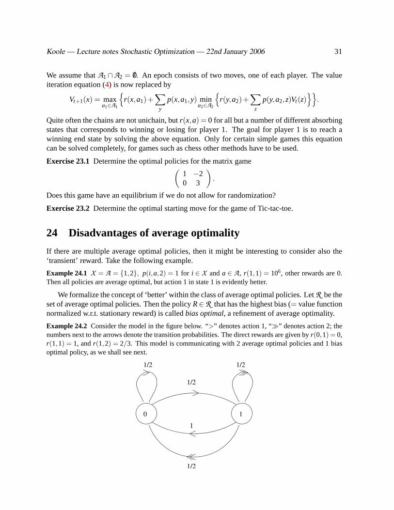
Example 24.2 Consider the model in the figure below. “>” denotes action 1, “�” denotes action 2; thenumbers next to the arrows denote the transition probabilities. The direct rewards are given byr(0,1) = 0,r(1,1) = 1, andr(1,2) = 2/3. This model is communicating with 2 average optimal policies and 1 biasoptimal policy, as we shall see next.

0 1

1

1/2

1/2

1/2

1/2


The optimality equation is as follows:

V(0)+g =12

V(0)+12

V(1);

V(1)+g = max{1+V(0),23

+12

V(0)+12

V(1)}.

The solutions are given by:

g = 1/3, V(0) = c, V(1) = 2/3+c, c∈ R.

The maximum is attained by actions 1 and 2, thus both possible policies (R1 = (1,1) andR2 = (1,2)) areaverage optimal. Do both policies have the same bias?

The bias BRi is the solution of the optimality equation with, additionally, the condition∑x πRi∗ (x)BRi (x) = 0. This assures that the bias of the stationary state is equal to 0. Reformulating the last

condition givesBRi = V−< πRi

∗ ,V > e.

Let us calculate the bias. TakeV = (0,2/3), the stationary distributions under both policies areπR1∗ =

(2/3,1/3), πR2∗ = (1/2,1/2). From that it follows thatBR1 = (−2/9,4/9) andBR2 = (−1/3,1/3). Thus

only R1 is bias optimal. The reason for this difference is thatπR1∗ 6= πR2

∗ .

Next we formulate a method to determine the bias optimal policy. Let(g,V) be a solution of

V +g = maxR:X→A

{r(R)+P(R)V},

andR = argmax{r +PV}, thesetof average optimal policies. We have to look for a policy inR that minimizes< πR

∗ ,V >. This is again an average reward problem, with optimality equation

V ′+g′ = maxR∈R{−V +P(R)V ′}.

The solution is the set of bias optimal policies, with biasV +g′.

Remark 24.3 This process can be repeated, to get reward as early as possible, etc. The remaining policyis equal to the limiting discount optimal policy.

The lack of focus on transient reward is not the only objection that can be made against thelong-run average reward as criterion: The focus on expectations is another one. Let us consideragain an example.

Example 24.4 Consider a model with rewards 1,1,1,1. . .; under the long-run average reward criterionthis cannot be distinguished from

with prob. 12: 0,0,0, . . . or 2,2,2, . . . ,

or at each point in time 0 or 2 with prob. 1/2.


The first and last example can occur in a single-class model, the middle one can only occurin a multi-class model. It has to do with the distribution of the average reward, of whichg isthe expectation. This distribution has hardly been studied in the literature. A possible way toconsider this type of problem is by decision trees.

Consider a single-class aperiodic model, the limiting average variance of policyR is givenby:

σ2(R) = limt→∞

E(r(Xt(R),At(R))−gR)2.

In terms of state-action frequencies:

σ2(R) =∑x,a

(r(x,a)−gR)2πR∗ (x,a).

BecausegR =∑

x,a r(x,a)πR∗ (x,a), we find

σ2(R) =∑x,a

(r2(x,a)−2r(x,a)gR+(gR)2

)πR∗ (x,a) =

∑x,a

r2(x,a)πR∗ (x,a)−

(∑x,a

r(x,a)πR∗ (x,a)

)2

.

Now we have a multi-criteria decision problem. We have the following possibilities forchoosing the objective:- maxR{gR|σ2(R)≤ α};- minR{σ2(R)|gR≥ α};- maxR{gR− γσ2(R)}.Note that all are risk-averse, i.e., the utility is concave. All problems are constrained Markovdecision problems with either a quadratic objective or a quadratic constraint, thus we have torely on mathematical programming to solve these problems.

Exercise 24.1Consider a discrete-time Markov decision process with states{0,1,2}, 2 ac-tions in 0 and 1 action in 1 and 2, and transition probabilitiesp: p(0,1,1) = p(0,2,2) = 2/3,p(0,1,2) = p(0,2,1) = 1/3, p(1,1,0) = p(2,1,0) = 1, and rewardsr equal to: r(1,1) = 1,r(0,2) = 1/3, r(0,1) = r(2,1) = 0.Compute the average reward, the bias and the average variance for both possible policies.Which policy would you prefer?

25 Monotonicity

For several reasons it can be useful to show certain structural properties of value functions.This can be used to characterize (partially) optimal policies, or it can be used as a first step incomparing the performance of different systems.


Admission control

Consider the value function of the M/M/1 queue with admission control (assuming thatλ+µ≤1), for rejection costsr and direct costsC(x) if there arex customers in the system:

Vn+1(x) = C(x)+λmin{r +Vn(x),Vn(x+1)}+µVn((x−1)+)+(1−λ−µ)Vn(x).

A threshold policyis a policy that admits customers up to a certain threshold value, above thatvalue customers are rejected. Whether or not the optimal policy for a certainn+1 is a thresholdpolicy depends on the form ofVn. The next theorem gives a sufficient condition.

Theorem 25.1 If Vn is convex, then a threshold policy is optimal for Vn+1.

Proof Vn convex means:2Vn(x+1)≤Vn(x)+Vn(x+2) for all x≥ 0,

and thusVn(x+1)− r−Vn(x)≤Vn(x+2)− r−Vn(x+1)

for all x≥ 0.If rejection is optimal inx, thus 0≤Vn(x+1)− r−Vn(x), then also 0≤Vn(x+2)− r−Vn(x+1), and

thus rejection is also optimal inx+1.

Theorem 25.2 If C and V0 are convex and increasing (CI), then Vn is CI for all n.

Proof By induction ton. SupposeVn is CI. This means

Vn(x)≤Vn(x+1) for all x≥ 0

2Vn(x+1)≤Vn(x)+Vn(x+2) for all x≥ 0

They can be used to show that the same inequalities hold forVn+1.

Corollary 25.3 If C is CI, then a threshold policy is optimal.

Proof Vn(x)−Vn(0) converges asn→ ∞ to a solutionV of the optimality equation and thusV is CI, andtherefore the average optimal policy is of threshold type.

A standard choice isC(x) = cx, which amounts toc holding costs for each unit of time that acustomer is in the system. If we takeC(x) = c(x−1)+, then only the customers in queue count.Note thatc(x−1)+ is convex (ifc≥ 0).

Remark 25.4 This result holds also for the M/M/s queue.


A server-assignment model

Consider next a model withmclasses of customers, arrival ratesλi and service ratesµi (maxi µi =µ,∑

i λi +µ≤ 1), a single server, and dynamic preemptive server assignment.The value function is as follows:

Vn+1(x) = C(x)+∑

i

λiVn(x+ei)+

mini{µiVn((x−ei)+)+(µ−µi)Vn(x)}+(1−

∑i

λi−µ)Vn(x).

Theorem 25.5 If c and V0 satisfy

µi f (x−ei)+(µ−µi) f (x)≤ µj f (x−ej)+(µ−µj) f (x)

for all x and i< j, xi > 0 and xj > 0 and

f (x)≤ f (x+ei)

for all x and i, then so do Vn for all n > 0.

Corollary 25.6 Under the above conditions a preemptive priority policy is optimal. In the spe-cial case that C(x) =

∑i cixi then the conditions are equivalent to ci ≥ 0 and µ1c1≥ ·· · ≥ µmcm,

resulting in the so-called µc-rule.

With this method many one and two-dimensional systems can be analyzed, but few multi-dimensional.

Remark 25.7 Note that other cost functions might lead to the same optimal policy. Whether or not thisis the case is checked by verifying if the conditions hold for the choice of cost function.

Exercise 25.1Consider theM/M/s/s queue with admission control with two classes of cus-tomers. Both classes have the same average service time, but differ in the reward per admittedcustomer.a. Formulate the backward recursion value function.b. Is the value function concave or convex? Show it.c. Consider a similar system but with rewards for each finished customer. How could you analyzethat?

Exercise 25.2Consider 2 parallel single-server queues with exponential service times, withequal rates. Customers arrive according to a Poisson process and are assigned in a dynamicway to the 2 queues. The objective is to minimize the average number of customers in the sys-tem.a. Formulate the backward recursion equation.b. Which relation onVn must hold for shortest queue routing to be optimal?c. Show that the value function is symmetric (i.e.,Vn(x,y) = Vn(y,x)).d. Prove by induction ton that shortest queue routing is optimal.


26 Incomplete information

The curse of dimensionality is not the only reason why Markov decision theory (or mathematicalmodeling in general) is little used in practice. There are two more reasons, that both are relatedto the same general concept ofincompleteor partial information. The first is that our methodsrequire all parameters to be given. This is in many cases an unrealistic assumption: parametersvary, depending on many other known and unknown underlying parameters. Therefore it is oftennot possible to give reliable estimates of parameters.

Example 26.1 A crucial parameter when optimizing a call center is the rate at which customers arrive.This parameter depends on many variables, some of which are known at the moment the planning is done(time of day, week of the year, internal events influencing the rate such as advertisement campaigns, etc.)and some of which are unknown (mainly external events such as weather conditions). This estimationissue is of major importance to call centers.

Next to unknown parameters it might occur that the state is not (completely) observed. Inprinciple the observation att can be any random function of the whole history of the system (thusincluding models with delay in observations), but usually it is a random function of the state att.

Example 26.2 In a telecommunication network decisions are made at the nodes of the system. In eachnode we often have delayed incomplete info on the other nodes. How to make for example decisionsconcerning the routing of calls?

Example 26.3 The state of a machine deteriorates when it is functioning, but we only known whether itis up or down. Timely preventive maintenance prevents expensive repairs after failure. When to schedulepreventive maintenance? What are the advantages ofcondition monitoring?

Example 26.4 In most card games we have partial information on the other hands.

The standard method in the case of unknown parameters is to observe the system first, esti-mate the parameters (the learning phase), and then control the system on the basis of the estimates(the control phase). The disadvantages are that we do not improve the system during the learningphase, and that we do not improve the parameter estimates during the control phase. This methodgets even worse if the parameters change over time, which is the rule in practice. Thus we needmore sophisticated methods.

There are several methods with each having their own advantages and disadvantages. Crucialto all these methods is that they do not first estimate and then control on the basis of theseestimates, but that while the system is being controlled the parameter estimations are improvedand with that the decisions. The simplest method, useful for example in the case of unknownarrival parameters consists of a standard statistical estimation procedure giving the most likelyvalue, followed by the execution of for example backward recursion at each time epoch using themost recent estimates. There are other methods in which the estimation and optimization stepscannot so easily be separated. One isQ-learning, in which the value function is updated usingideas from stochastic approximation. It is useful in the case that nothing is known about thetransition probabilities, it is a method that makes no initial assumptions. A mathematically more


sophisticated and numerically more demanding method is Bayesian dynamic programming, forwhich an initial (“prior”) distribution of the unknown parameters is needed.

Note that also approximate dynamic programming can be used for problems with uncompleteinformation. We made no assumptions on the transition structure, and therefore it can also beused for the partial-information case. As for Q-learning no initial distribution is needed.

Remark 26.5 If we consider just the average long-run reward then learning over a (very) long period andthen controlling is (almost) optimal. The disadvantage is the loss of reward during the learning phase, seethe discussion of disadvantages of the average reward criterion in Section24. For this reason we mainlylook at discounted rewards. Another problem is the issue of parameters varying slowly over time. Thenwe can never stop learning, and learning and control have to be done simultaneously.

Exercise 26.1Consider anM/M/1 queue with admission control, thus arriving customers maybe rejected. Every customer in queue costs 1 unit per time holding costs, but every admittedcustomer gives a rewardr. It is the objective to maximize the discounted revenue minus holdingcosts. The arrival rate is 1, but the service rate is unknown.a. Give a procedure to estimate the parameter of the service time distribution on the basis of therealizations up to now.b. How would you use this to design a control algorithm for this model?c. Implement a computer program that repeats the following experiment a number of times: drawthe service rate from a homogeneous[0,2] distribution, and simulate the queue with admissionwith the algorithm of part b implemented. Report on it for a few choices of parameters.d. Compare the results of c to the model where the service rate is known from the beginning.

Q-learning

Q-learning is a method that is suitable for systems of which the state is observed, but no infor-mation is known about the transition probabilities, not even the structure.

We will work with a model with discounting (with parameter,β ∈ [0,1)), in discrete time.We allow the reward to depend on the new state, thusr is of the formr(x,a,y) with x the currentstate,a the action, andy the new state.

The value function is then given by:

V(x) = maxa{∑

y

p(x,a,y)[r(x,a,y)+βV(y)]}.

DefineQ(x,a) =

∑y

p(x,a,y)[r(x,a,y)+βV(y)].

ThenQ(x,a) =

∑y

p(x,a,y)[r(x,a,y)+βmaxa

Q(y,a)].

This gives an alternative way for calculating optimal policies.


Now we move to systems with unknown parameters, and we assume that a simulator exists:we have a system for which it is possible to draw transitions according to the correct probabilitylaws, but it is too time consuming to calculate transition probabilities (otherwise standard valueiteration would be preferable).

Let ξn(x,a) ∈ X be the outcome of the simulation at stagen, for statex and actiona. Let bn

be a series with ∑n

bn = ∞,∑

n

b2n < ∞.

TheQ-learning algorithm works as follows:

Qn+1(x,a) = (1−bn)Qn(x,a)+bnmaxa

[r(x,a,ξn(x,a))+βQn(ξn(x,a),a)].

Then:Qn→Q, and thus in the limit the algorithm gives the optimal actions.

Remark 26.6 If the system is controlled in real time, then the algorithm is executed in an asynchronousway: onlyQ(x,a) is updated for the currentx anda. This has the risk that certain(x,a) combinations neverget updated. Therefore sub-optimal actions should also be chosen to give the algorithm the possibility tolearn on all(x,a) combinations.

Remark 26.7 Why did we take∑

nbn = ∞ and∑

nb2n < ∞? If

∑nbn < ∞ then there is no guaranteed

convengence to the right value (e.g.,bn ≡ 0). On the other hand, if∑

nb2n = ∞, then there need not be

convengence (e.g.,bn≡ 1). The usual choice ofbn is bn = 1n.

See also the Robbins-Monro stochastic approximation algorithm.

Bertsekas & Tsitsiklis [4] gives more information onQ-learning.

Exercise 26.2Consider the model of Exercise26.1. Is it useful to applyQ-learning to thismodel? Motivate your answer.

Bayesian dynamic programming

In Bayesian dynamic programming we make a difference between the state of the model (withstate spaceX ) and the state of the algorithm (theinformation state) that represents the informa-tion we have. The information state is actually a distribution on the set of model states. Thisinformation state holds all information on all observations up to the current time. Thus it is ob-servable, it only depends on the observations, and the Markov property holds: all informationabout the past is used. Thus (see Section17) the information state can be used to solve theproblem.

Starting with some well-chosen prior, the information state is updated every time unit usingBayes’ rule. This gives the optimal policy, given the initial distribution. Note however thatfor state spaceX the information state space is given by[0,1]|X |, thus an|X |-dimensional statespace, which each variable a probability. ThusX is not even countable, we will certainly haveto discretizethe state space to make computations possible. Even for small state spaces and acoarse discretization of the interval[0,1] this quickly leads to unfeasible state space sizes.


Let us formalize the framework. Next to the state spaceX we have anobservation spaceZ. With q(x,z) we denote the probability of observingz∈ Z in x ∈ X . Next we define theinformation states, which are thus distributions onX : P = [0,1]X (in case|X | countable).

Consideru∈ P . For eachz∈ Z there is a transition to a new statev∈ P ; for observationzthe distributionv is defined by

v(y) = P(now aty|before atu, a chosen,z observed) =∑

xu(x)p(x,a,y)q(y,z)∑x

∑yu(x)p(x,a,y)q(y,z)

,

and thus the transition probabilities are given by

p′(u,a,v) =∑

x

∑y

u(x)p(x,a,y)q(y,z).

Here we assumed that foru different observations lead to differentv; if this is not the case thenthe transition probabilities should be added.

Example 26.8 A service center is modeled as a single-server queue. We have the option to send customersto another center when the queue gets too long (admission control). We assume that the capacity ofthe queue isN: aboveN customers balk automatically. The partial-information aspect is that we donot observe the queue, we only observe whether or not the server is busy. The state is the number ofcustomers in the system,X = {0,1,2, . . . ,N}, action setA = {0,1} representing rejection and admission.The observation is 1 (0) is the server is busy (idle),Z = {0,1}, andq(x,1) = 1 for x > 0, q(0,0) = 1.Every state is a vector withN +1 probabilities. Letu∈ P , and letλ andµ be the uniformized transitionparameters,λ+µ= 1. Thenp′(u,a,e0) = λI{a= 0}u(0)+µ(u(0)+u(1)). The second possible transitionis p′(u,a,v) = 1− p′(u,a,e0) with

v(y) =λI{a = 0}u(y)+λI{a = 1}u(y−1)+µu(y+1)

1−λI{a = 0}u(0)−µu(1),

for y > 0 (we assume thata = 0 is chosen in stateN). It can probably be shown thatv is stochasticallyincreasing in the number of times that 1 is observed since the last observation of 0. From this we concludethat an optimal policy rejects from a certain number of consecutive observations of 1 on. See [11] for asimilar result.

Example 26.9 Suppose there are several different medical treatment for a certain illness, each with un-known success probability. How to decide which treatment to use for each patient?

At first sight this can be translated in a one-state model. However, the reward depends on the successprobability of the chosen treatment. Thus the success probabilities should be part of the state space.

Suppose there are two possible treatments, then the state is represented by the tuple(θ1,θ2), giving thesuccess probabilities of the two treatments. However, this state is unobserved: instead of this we have asinformation state a tuple of distributions on[0,1]. Each time unit a new patient arrives, the question is howto treat this patient. This question can be answered by solving a Markov decision problem with as statespace all possible tuples of independent 0-1 distributions. ThusX = [0,1]2, A = {1,2}, the treatmentto be used,Z = {0,1}, the result of the treatment (1 means success). BecauseX is a continuous set,

information states are densities:P = (R[0,1]+ ,R[0,1]

+ ), tuples of densities, both on the probabilities[0,1].


Takeu = (u1,u2). For actiona only ua is updated. Considera = 1 (the casea = 2 is equivalent). Then asuccess occurs with probability

∫ 10 xu1(x)dx, and the resulting information state isv= (v1,v2) with v2 = u2

andv1 defined by

v1(y) =yu1(y)∫ 1

0 xu1(x)dx

in case of a success (which occurs thus with probability∫ 1

0 xu1(x)dx), andv1 such that

v1(y) =(1−y)u1(y)∫ 1

0 (1−x)u1(x)dx

in case of a failure (with probability∫ 1

0 (1−x)u1(x)dx).Using this in an optimization algorithm is computationally infeasable, therefore we have to look for a

method to reduce the size of the state space. That we will discuss next. See [5] for more information onthis example.

In the examples we saw that in partial-information problems the state space very quicklybecomes so big that direct computation of optimal policies is infeasable. In the first example wesaw that instead of working with all distributions we can work with the time until the last timethe system was empty. This is a much simpler representation of the state space. For systems withunknown parameters such a simpler representation of the information states exists sometimesas well. In such cases the densities that occur as information states fall into a certain class ofparametrized families, such as Beta distributions. The crucial property is that the distributionshould be closed under the Bayesian update. We will show that this is the case in the setting ofExample26.9.

Let us introduce the class of Beta distributions. A Beta(k, l) distribution has densityf (x) ∝xk(1−x)l . Note that fork = l = 0 we find the uniform distribution on[0,1].

Theorem 26.10Consider a Bernoulli random variable X with parameterθ that has a Beta(k, l)distribution. Thenθ|X = 1 (the a posteriori distribution) has a Beta(k+1, l) distribution;θ|X =0 has a Beta(k, l +1) distribution.

Proof We have:

P(x≤ θ≤ x+h|X = 1) =P(x≤ θ≤ x+h,X = 1)

P(X = 1)=

P(x≤ θ≤ x+h)P(X = 1|x≤ θ≤ x+h)P(X = 1)

.

Dividing by h and taking the limit ash→ 0 gives (with fX denoting the density ofX):

fθ|X=1(x) =fθ(x)P(X = 1|θ = x)

P(X = 1)=

fθ(x)xP(X = 1)

.

becausefθ(x) = C(k, l)xk(1− x)l we find indeed thatθ|X = 1 has densityCxk+1(1− x)l , with C =C(k, l)/P(X = 1). A similar argument applies to the caseX = 0.


This theorem is very useful for Example26.9: we can replace the densities by two-dimensional discrete variables, resulting for the problem with two possible treatment in fourvariables. It is crucial to start with an initial Beta distributed belief (the prior) for each treatment,for example each having a uniform distribution. Crucial here is that if we start with a uniformprior, then all distributions are Beta distributions which can be characterized by two discrete pa-rameters. Thus under a Beta-distributed prior the problem is 4-dimensional and can be solvedusing backward recursion.

Two types of distributions, where one is the parameter of the other and one remains withinthe same class of distributions after a Bayesain update, are calledconjugate distributions(seeDeGroot [7]).

Exercise 26.3Consider a machine that detects certain rare particles. At discrete points in timeit can give a signal or not. When it gives a signal, it is functioning and it has detected a particle.When it does not give a signal, it is either broken down or there was no particle. Every timeunit there is a particle with probabilityp, and when it is functioning the machine breaks downwith probabilityq. To replace a machine that is broken down a new one has to be bought. Theobjective is to have a working machine as often as possible for as little money as possible.a. Describe the states and the transition probabilities of this system if it is observed when themachine breaks down. What is a reasonable policy?b. Describe the information states and the transition probabilities of this system if it cannot beobserved when the machine is down. What is a reasonable policy?

Exercise 26.4We observe a realizationy of an exponentially distributed random variable thathas a parameter that is gamma(n,α) distributed. What is the a posteriori distribution of theparameter?

Acknowledgments

I thank Sandjai Bhulai for his many remarks and suggestions.

References

[1] E. Altman.Constrained Markov Decision Processes. Chapman and Hall, 1999.

[2] R. Bellman.Adaptive Control Processes: A Guided Tour. Princeton University Press, 1961.

[3] D.P. Bertsekas.Dynamic Programming. Prentice-Hall, 1987.

[4] D.P. Bertsekas and J.N. Tsitsiklis.Neuro-Dynamic Programming. Athena Scientific, 1996.

[5] S. Bhulai and G.M. Koole. On the value of learning for Bernoulli bandits with unknownparameters.IEEE Transactions on Automatic Control, 45:2135–2140, 2000.

[6] E. Cinlar. Introduction to Stochastic Processes. Prentice-Hall, 1975.


[7] M.H. DeGroot.Optimal Statistical Decisions. McGraw-Hill, 1970.

[8] M. El-Taha and S. Stidham, Jr.Sample-Path Analysis of Queueing Systems. Kluwer, 1998.

[9] R. Groenevelt, G.M. Koole, and P. Nain. On the bias vector of a two-class preemptivepriority queue.Mathematical Methods of Operations Research, 55:107–120, 2002.

[10] L.C.M. Kallenberg. Finite state and action MDPs. In E.A. Feinberg and A. Shwartz, editors,Handbook of Markov Decision Processes, pages 21–86. Kluwer, 2002.

[11] G.M. Koole. On the static assignment to parallel servers.IEEE Transactions on AutomaticControl, 44:1588–1592, 1999.

[12] T.J. Ott and K.R. Krishnan. Separable routing: A scheme for state-dependent routing ofcircuit switched telephone traffic.Annals of Operations Research, 35:43–68, 1992.

[13] M.L. Puterman.Markov Decision Processes. Wiley, 1994.

[14] S.M. Ross.Introduction to Stochastic Dynamic Programming. Academic Press, 1983.

[15] D.R. Smith. Dynamic programming and board games. Unpublished,www.maths.ex.ac.uk/∼DKSmith/if16pape.pdf, 1999.

[16] H.C. Tijms. Stochastic Modelling and Analysis: A Computational Approach. Wiley, 1986.

http://www.maths.ex.ac.uk/~DKSmith/if16pape.pdf

Documents

Lecture Notes Stochastic Optimization-Koole