Embed Size (px)
Citation preview

CS – 590.21 Analysis and Modeling of Brain NetworksDepartment of Computer Science
University of Crete
Lecture on Modeling Tools for Null Hypothesis Testing & Correlation

Acknowledgement – Resources used in the slides
On statistical hypothesis test• Yiannis Tsamardinos (University of Crete)
• William Morgan (Stanford University)
On clustering
• Jiawei Han, University of Illinois at Urbana-Champaign

Agenda
Basic data analysis & modeling tools that can be employed in the projects
• Null Hypothesis Test
• Temporal correlation metrics
• Pearson correlation
• STTC
• Kolmogorov-Smirnov Test
• Clustering
k-means
• Regression
• Linear regression
• Lasso & Ridge regression
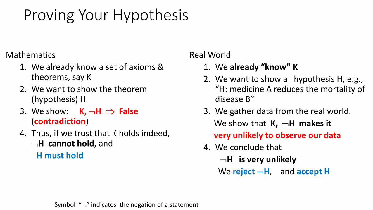
Proving Your Hypothesis
Mathematics
1. We already know a set of axioms &theorems, say K
2. We want to show the theorem (hypothesis) H
3. We show: K, H False (contradiction)
4. Thus, if we trust that K holds indeed, H cannot hold, and
H must hold
Real World
1. We already “know” K
2. We want to show a hypothesis H, e.g., “H: medicine A reduces the mortality of disease B”
3. We gather data from the real world.
We show that K, H makes it
very unlikely to observe our data
4. We conclude that
H is very unlikely
We reject H, and accept H
Symbol “” indicates the negation of a statement
Notation for the following slides
• Random variables are denoted with a capital letter, e.g., X
• Observed quantities of random variables are denoted with their corresponding small letter x
Example:• G is the expression level of a specific gene in a patient
• g is the measured expression level of the game in a specific patient
The Null Hypothesis
• The hypothesis we hope to accept is called the Alternative Hypothesis
Sometimes denoted as H1
• The hypothesis we hope to reject, the negation of the Alternative Hypothesis, is called the Null Hypothesis
Usually denoted by Ho
Think of the Ho as the “status quo”
Standard Single Hypothesis Testing
1. Form the Null & Alternative Hypothesis
2. Obtain related data
3. Find a suitable test statistic T
4. Find the distribution of T given the null
5. Depending on the distribution of T & the observed to = T ( x)
decide to reject or not H0
Test Statistics
• Test statistic is a function of our data X: T(X) ( X: random variable )e.g., if X contains a single quantity (variable) T(X) the mean value of X
• T is a random variable (since it depends on X , our data which is random variable)
• Denote with to = T(x) the observed value of T in our data
• Instead of calculating P ( obtaining data similar to X | H0 )
Calculate P ( T similar to to | H0 )
• If P ( T similar to to | H0) is very low, reject H0
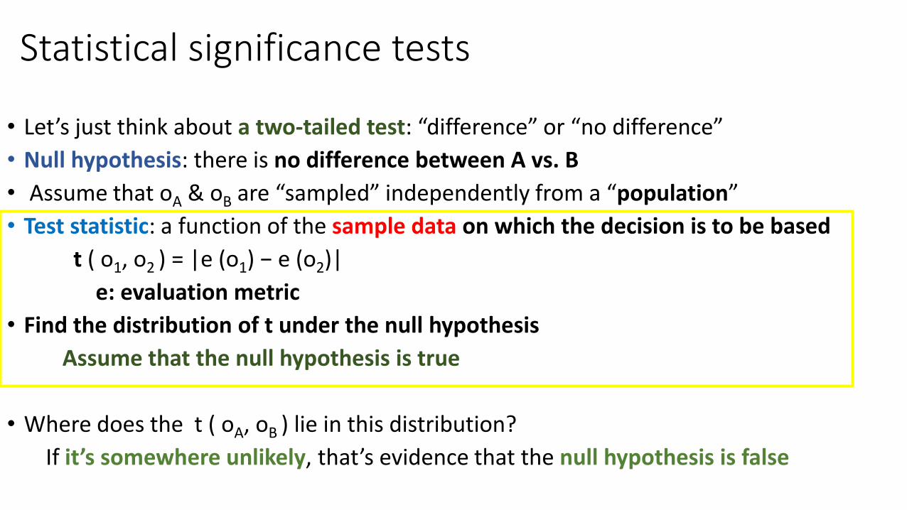
Statistical significance tests
• Let’s just think about a two-tailed test: “difference” or “no difference”
• Null hypothesis: there is no difference between A vs. B
• Assume that oA & oB are “sampled” independently from a “population”
• Test statistic: a function of the sample data on which the decision is to be based
t ( o1, o2 ) = |e (o1) − e (o2)|
e: evaluation metric
• Find the distribution of t under the null hypothesis
Assume that the null hypothesis is true
• Where does the t ( oA, oB ) lie in this distribution?
If it’s somewhere unlikely, that’s evidence that the null hypothesis is false

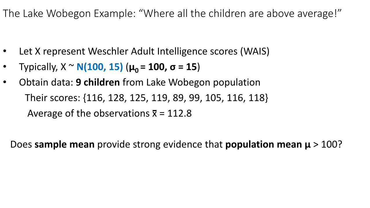
The Lake Wobegon Example: “Where all the children are above average!”
• Let X represent Weschler Adult Intelligence scores (WAIS)
• Typically, X ~ N(100, 15) (μ0 = 100, σ = 15)
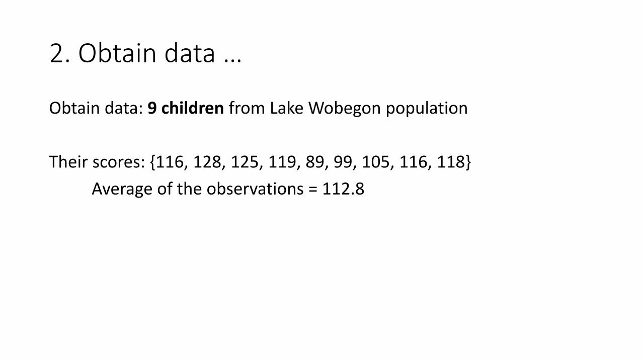
• Obtain data: 9 children from Lake Wobegon population
Their scores: {116, 128, 125, 119, 89, 99, 105, 116, 118}
Average of the observations x = 112.8
Does sample mean provide strong evidence that population mean μ > 100?
-
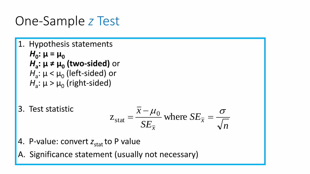
One-Sample z Test
1. Hypothesis statementsH0: µ = µ0Ha: µ ≠ µ0 (two-sided) or Ha: µ < µ0 (left-sided) orHa: µ > µ0 (right-sided)
3. Test statistic
4. P-value: convert zstat to P value
A. Significance statement (usually not necessary)
nSE
SE
xx
x
where z 0
stat
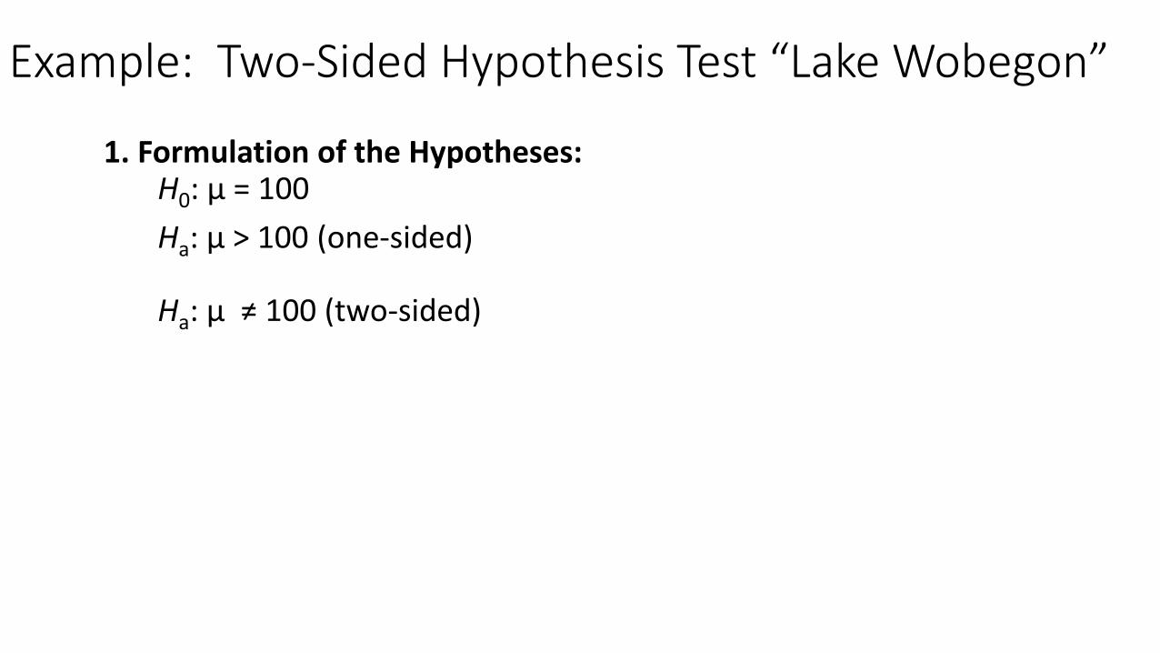
Example: Two-Sided Hypothesis Test “Lake Wobegon”
1. Formulation of the Hypotheses: H0: μ = 100
Ha: µ > 100 (one-sided)
Ha: µ ≠ 100 (two-sided)
2. Obtain data …
Obtain data: 9 children from Lake Wobegon population
Their scores: {116, 128, 125, 119, 89, 99, 105, 116, 118}
Average of the observations = 112.8

Example: Two-Sided Hypothesis Test “Lake Wobegon”
3. Test statistic
56.25
1008.112
59
15
0stat
x
x
SE
xz
nSE
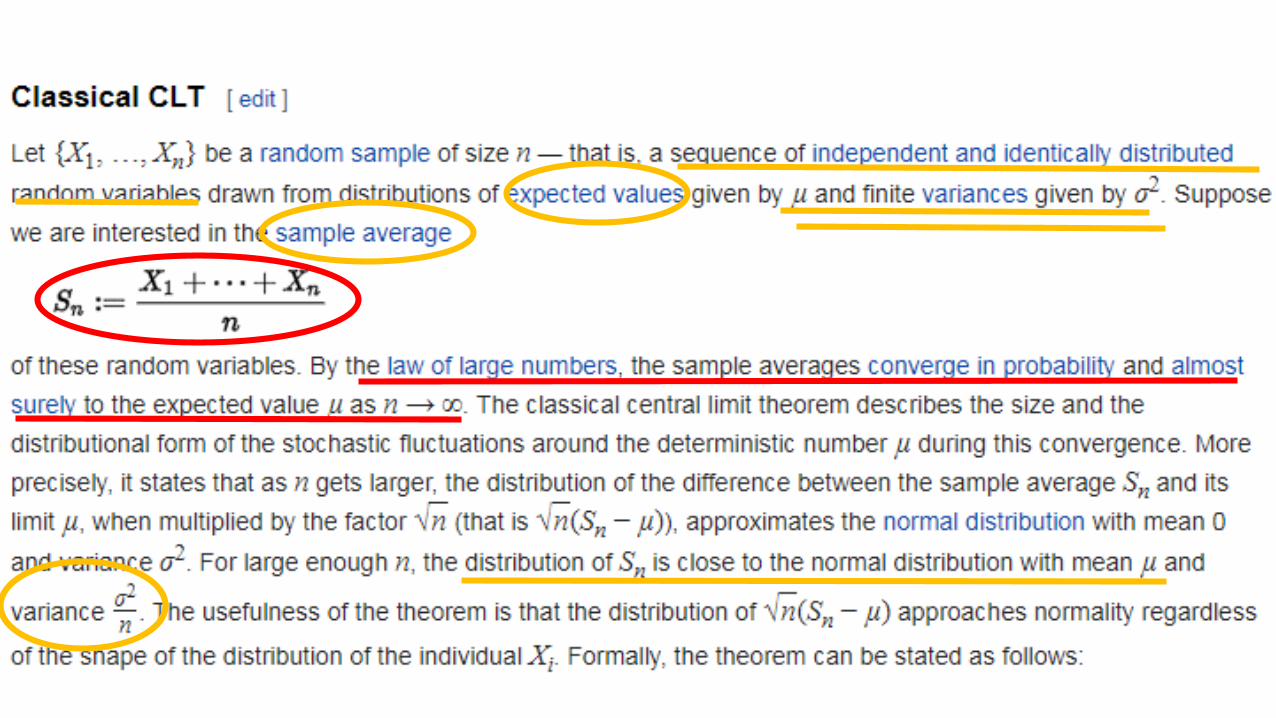
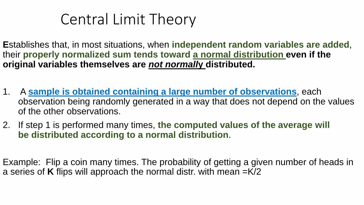
Central Limit Theory
Establishes that, in most situations, when independent random variables are added, their properly normalized sum tends toward a normal distribution even if the original variables themselves are not normally distributed.
1. A sample is obtained containing a large number of observations, each observation being randomly generated in a way that does not depend on the values of the other observations.
2. If step 1 is performed many times, the computed values of the average will be distributed according to a normal distribution.
Example: Flip a coin many times. The probability of getting a given number of heads in a series of K flips will approach the normal distr. with mean =K/2
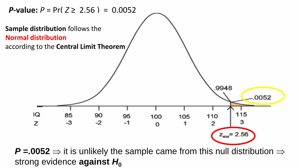
P-value: P = Pr( Z ≥ 2.56 ) = 0.0052
P =.0052 it is unlikely the sample came from this null distribution
strong evidence against H0
Sample distribution follows the Normal distributionaccording to the Central Limit Theorem
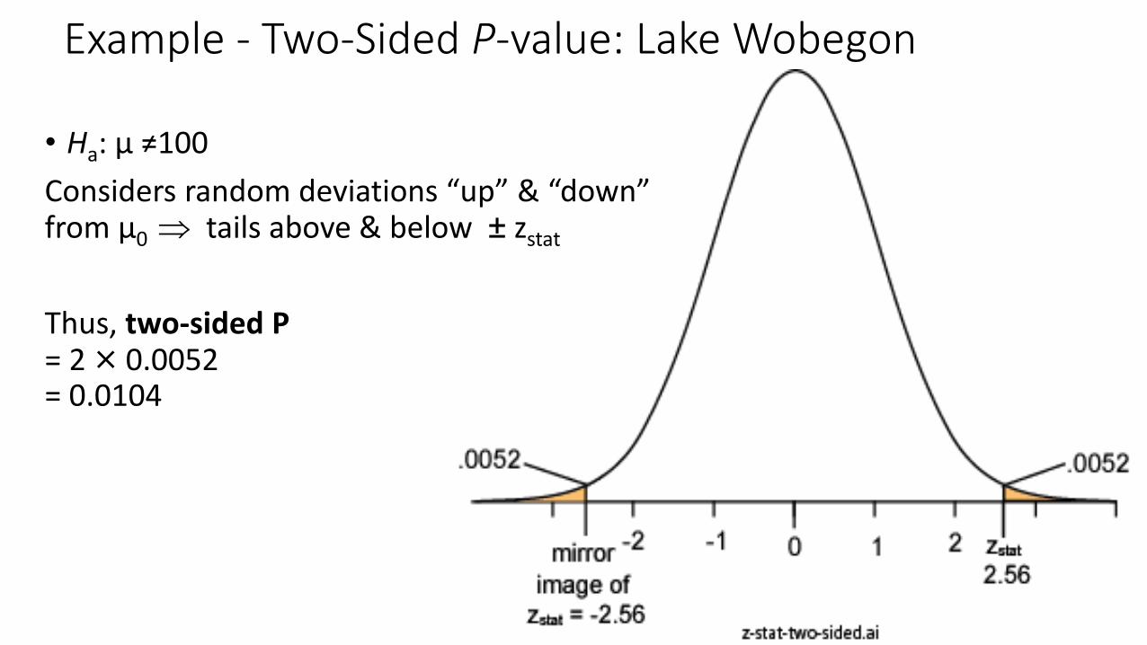
• Ha: µ ≠100
Considers random deviations “up” & “down” from μ0 tails above & below ± zstat
Thus, two-sided P = 2 × 0.0052 = 0.0104
Example - Two-Sided P-value: Lake Wobegon
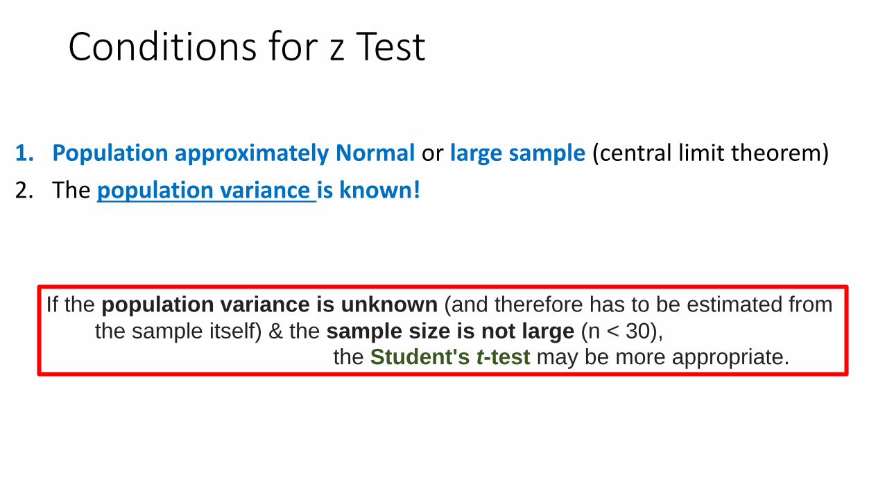
Conditions for z Test
1. Population approximately Normal or large sample (central limit theorem)
2. The population variance is known!
If the population variance is unknown (and therefore has to be estimated from
the sample itself) & the sample size is not large (n < 30), the Student's t-test may be more appropriate.

Another Example
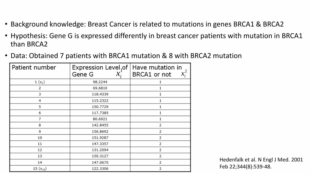
• Background knowledge: Breast Cancer is related to mutations in genes BRCA1 & BRCA2
• Hypothesis: Gene G is expressed differently in breast cancer patients with mutation in BRCA1than BRCA2
• Data: Obtained 7 patients with BRCA1 mutation & 8 with BRCA2 mutation
Hedenfalk et al. N Engl J Med. 2001 Feb 22;344(8):539-48.
1
ix 2
ix
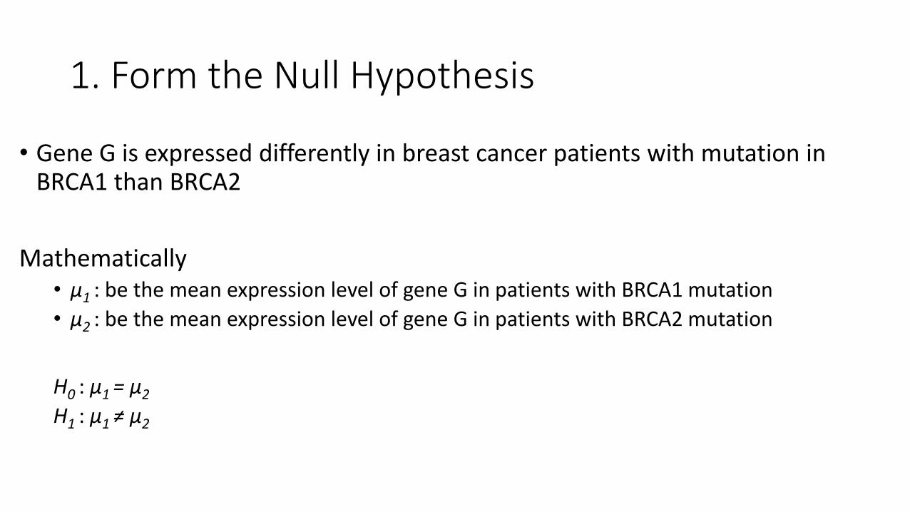
1. Form the Null Hypothesis
• Gene G is expressed differently in breast cancer patients with mutation in BRCA1 than BRCA2
Mathematically• μ1 : be the mean expression level of gene G in patients with BRCA1 mutation
• μ2 : be the mean expression level of gene G in patients with BRCA2 mutation
H0 : μ1 = μ2
H1 : μ1 ≠ μ2
2. Obtain data….
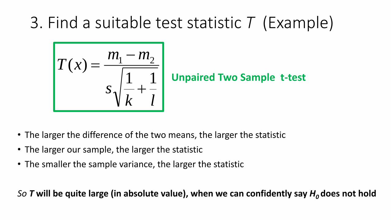
3. Find a suitable test statistic T (Example)
lks
mmxT
11)( 21
• The larger the difference of the two means, the larger the statistic
• The larger our sample, the larger the statistic
• The smaller the sample variance, the larger the statistic
So T will be quite large (in absolute value), when we can confidently say H0 does not hold
Unpaired Two Sample t-test
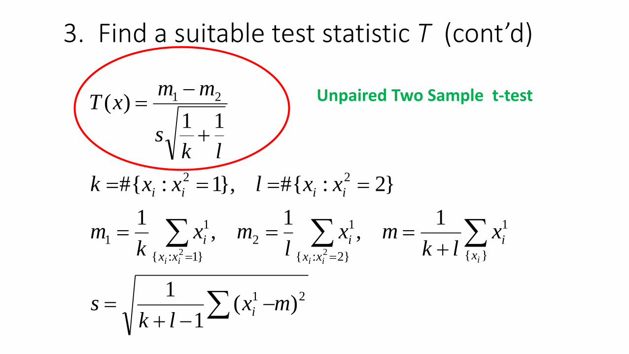
3. Find a suitable test statistic T (cont’d)
21
}{
1
}2:{
1
2
}1:{
1
1
22
21
)(1
1
1,
1,
1
}2:{#},1:{#
11)(
22
mxlk
s
xlk
mxl
mxk
m
xxlxxk
lks
mmxT
i
x
i
xx
i
xx
i
iiii
iiiii
Unpaired Two Sample t-test
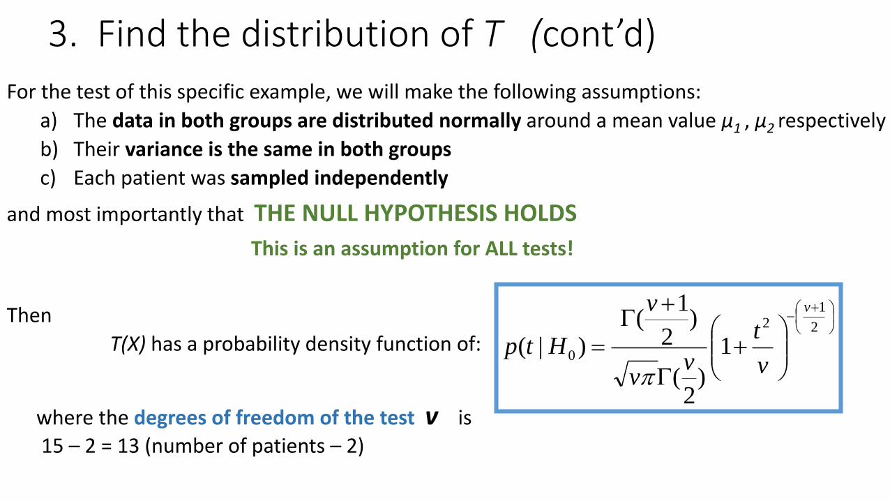
3. Find the distribution of T (cont’d)
For the test of this specific example, we will make the following assumptions:
a) The data in both groups are distributed normally around a mean value μ1 , μ2 respectively
b) Their variance is the same in both groups
c) Each patient was sampled independently
and most importantly that THE NULL HYPOTHESIS HOLDS
This is an assumption for ALL tests!
Then
T(X) has a probability density function of:
2
12
0 1
)2
(
)2
1(
)|(
v
v
t
vv
v
Htp
where the degrees of freedom of the test v is
15 – 2 = 13 (number of patients – 2)
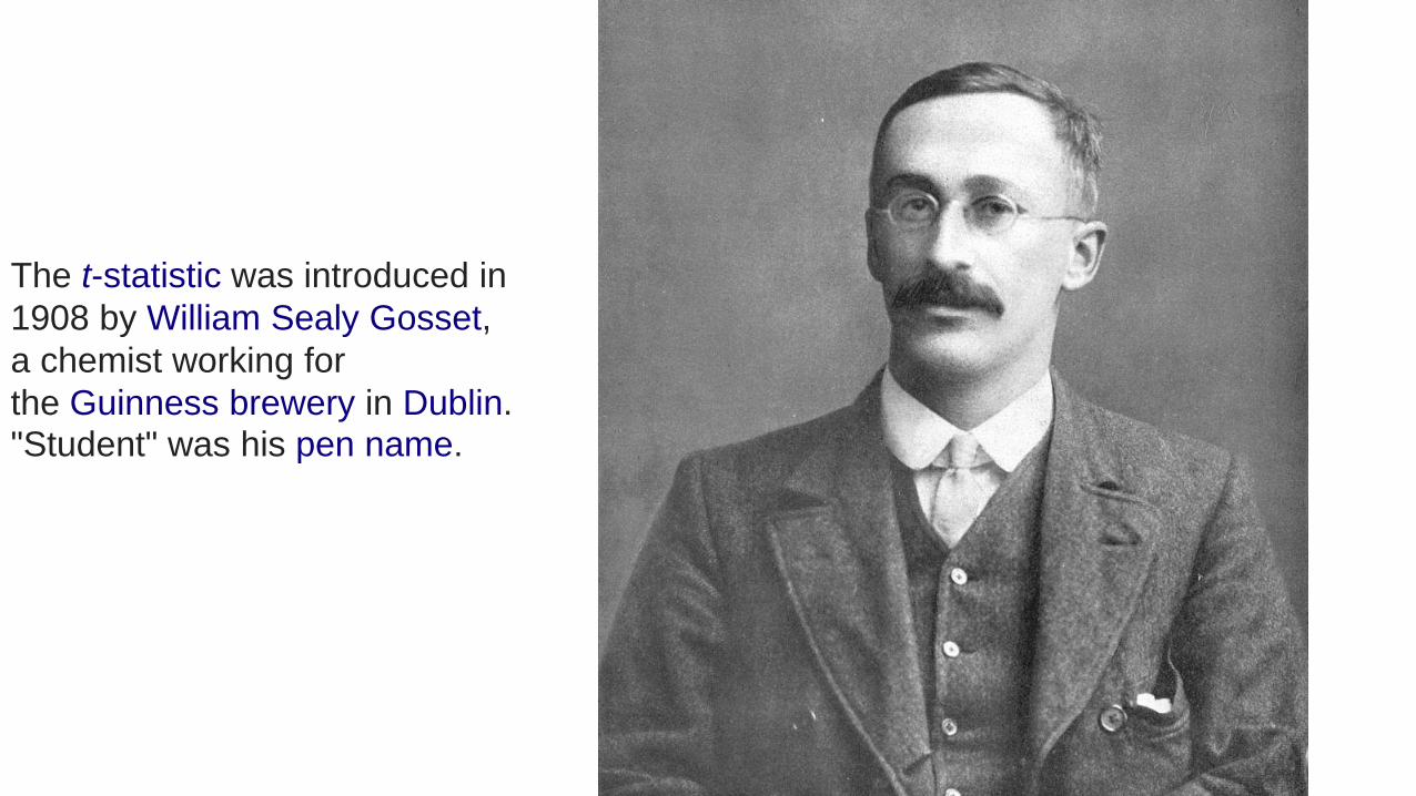
The t-statistic was introduced in
1908 by William Sealy Gosset,
a chemist working for
the Guinness brewery in Dublin. "Student" was his pen name.
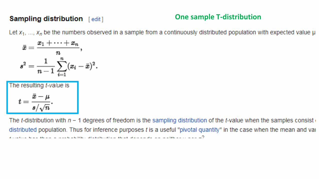
One sample T-distribution
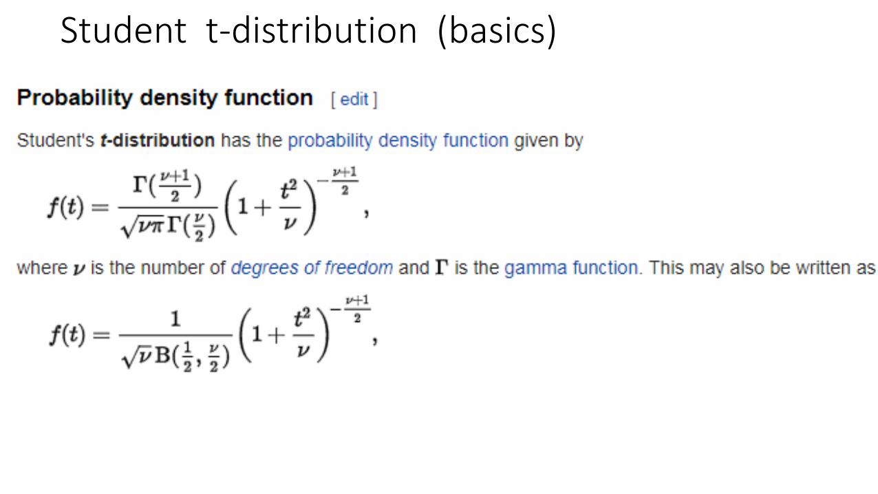
Student t-distribution (basics)
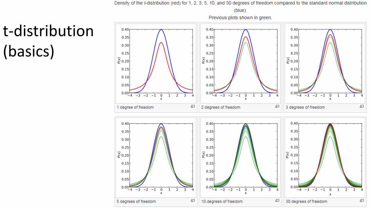
t-distribution (basics)
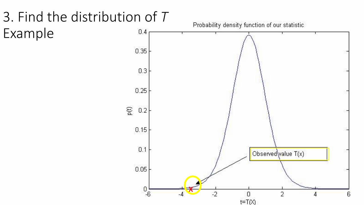
3. Find the distribution of TExample
x
4. Decide on a Rejection Region
• Decide on a rejection region Γ in the range of our statistic
• If to Γ , then reject H0
• If t o Γ , then do not reject H0
accept H1 ?
Since the pdf of T when the null hypothesis holds is known,
P( T Γ | H0 ) can be calculated
4. Decide on a Rejection Region
• If P( T Γ | H0 ) is too low, we know we are safely rejecting H0
• What should be our rejection region in our example?
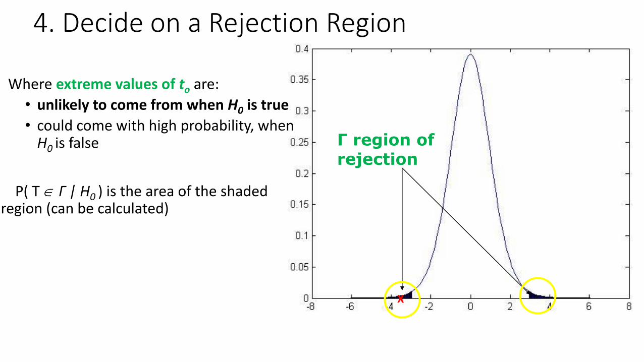
Γ region of rejection
4. Decide on a Rejection Region
Where extreme values of to are:
• unlikely to come from when H0 is true
• could come with high probability, when H0 is false
P( T Γ | H0 ) is the area of the shaded region (can be calculated)
X
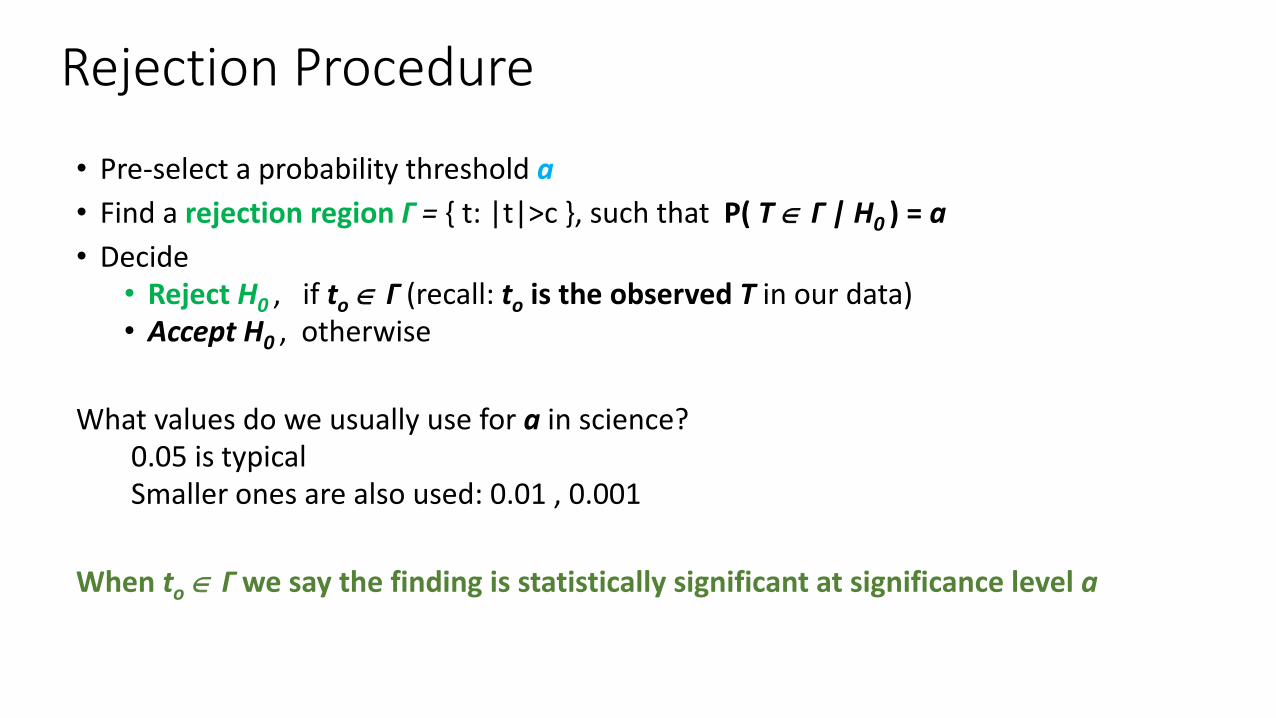
Rejection Procedure
• Pre-select a probability threshold a
• Find a rejection region Γ = { t: |t|>c }, such that P( T Γ | H0 ) = a
• Decide• Reject H0 , if to Γ (recall: to is the observed T in our data)• Accept H0 , otherwise
What values do we usually use for a in science?0.05 is typical Smaller ones are also used: 0.01 , 0.001
When to Γ we say the finding is statistically significant at significance level a
Copyright (c) 2004 Brooks/Cole, a division of Thomson Learning, Inc.
Issues to be Considered
• When there exist two or more tests that are appropriate in a given situation,
how can the tests be compared to decide which should be used?
• If a test is derived under specific assumptions about the distribution of the
population being sampled,
how well will the test procedure work when the assumptions are violated?
Parametric versus non-Parametric Tests
• Parametric test
Makes the assumption that the data are sampled from a particular class of distributions
It then becomes easier to derive the distribution of the test statistic
• Non-Parametric test
No assumption about a particular class of distributions
Permutation Testing
• Often in biological data, we do not know much about the data distribution
• How do we obtain the distribution of our test statistic?
• Great idea in statistics: permutation testing
• Recently practical because it requires computing power (or a lot of patience)
Permutation Testing
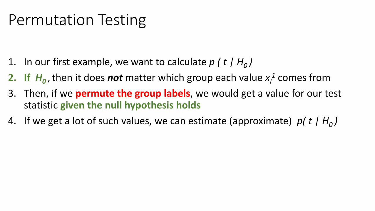
1. In our first example, we want to calculate p ( t | H0 )
2. If H0 , then it does not matter which group each value xi1 comes from
3. Then, if we permute the group labels, we would get a value for our test statistic given the null hypothesis holds
4. If we get a lot of such values, we can estimate (approximate) p( t | H0 )
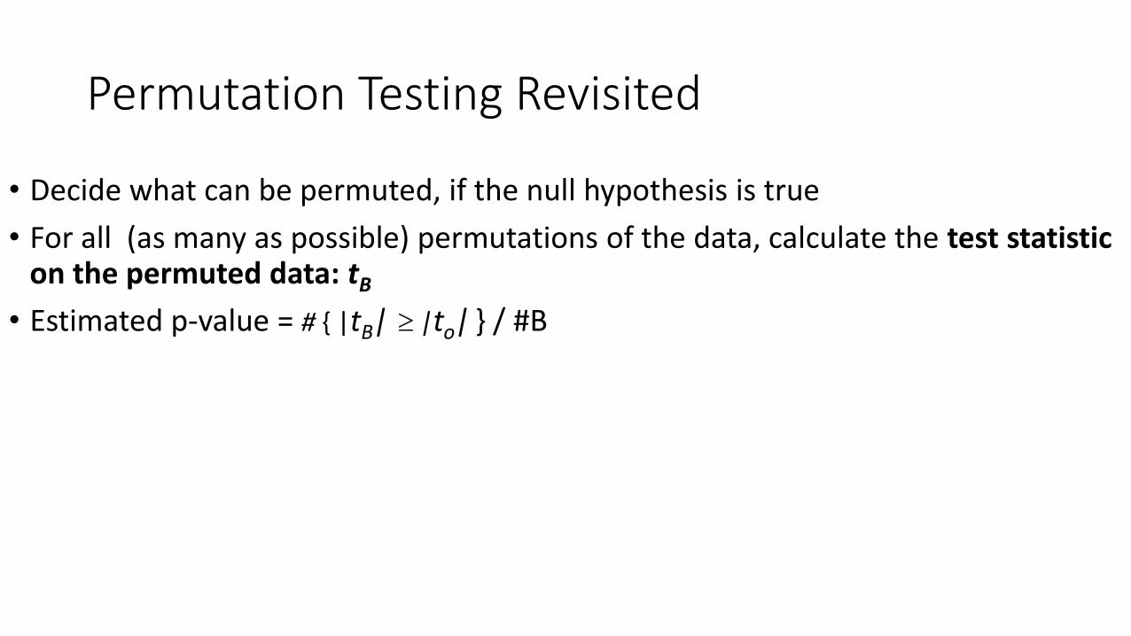
Permutation Testing Revisited
• Decide what can be permuted, if the null hypothesis is true
• For all (as many as possible) permutations of the data, calculate the test statistic on the permuted data: tB
• Estimated p-value = # { |tB| |to| } / #B
True distribution calculated theoretically
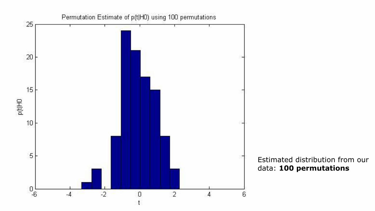
Estimated distribution from our data: 100 permutations
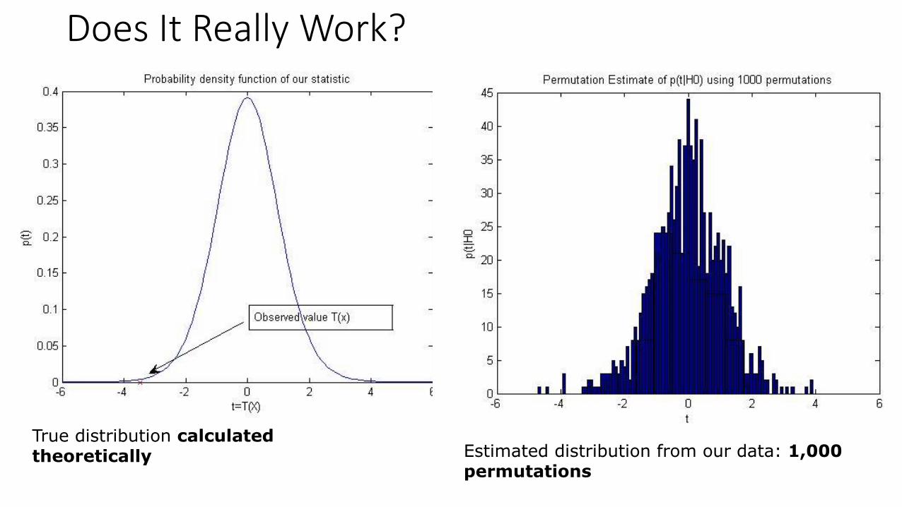
Does It Really Work?
True distribution calculated theoretically Estimated distribution from our data: 1,000
permutations
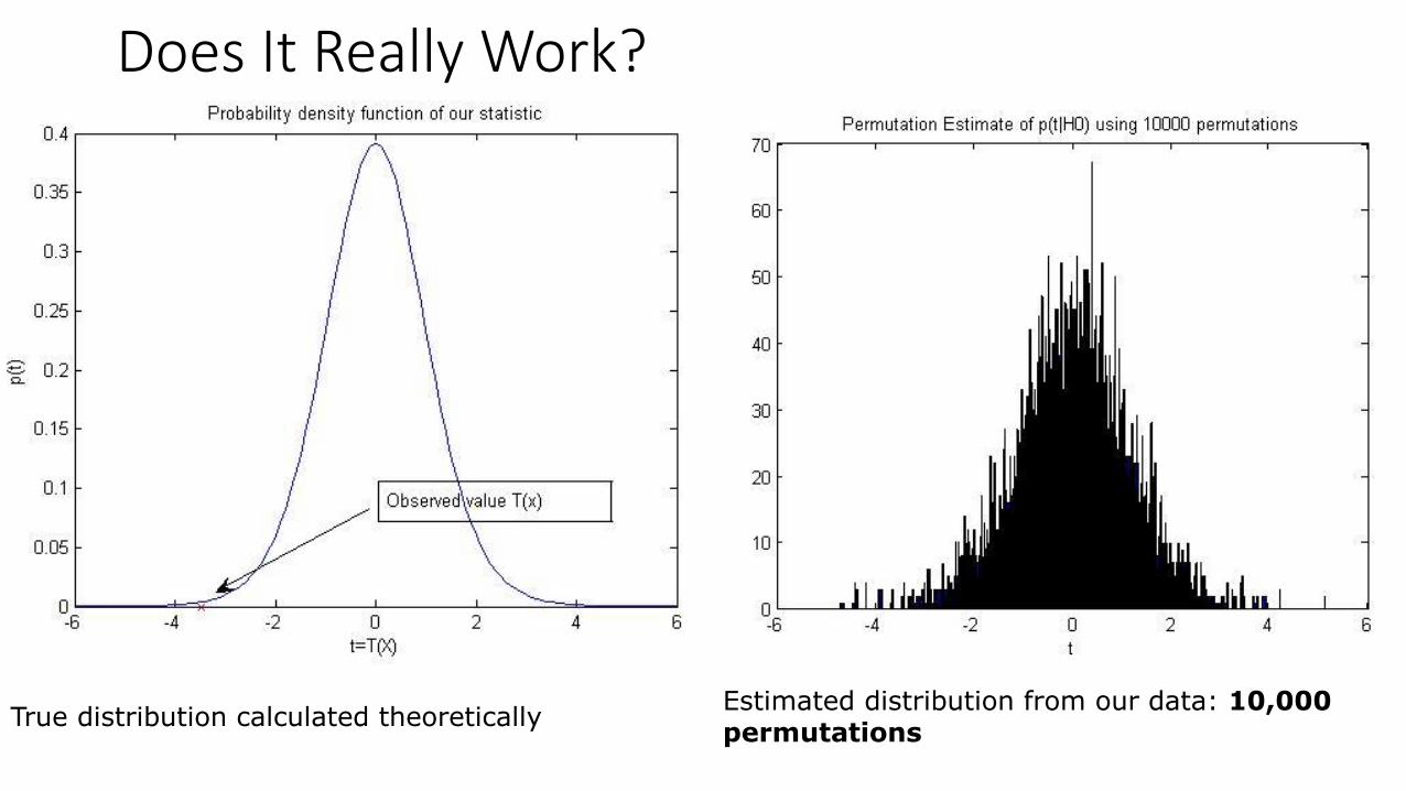
Does It Really Work?
True distribution calculated theoreticallyEstimated distribution from our data: 10,000 permutations
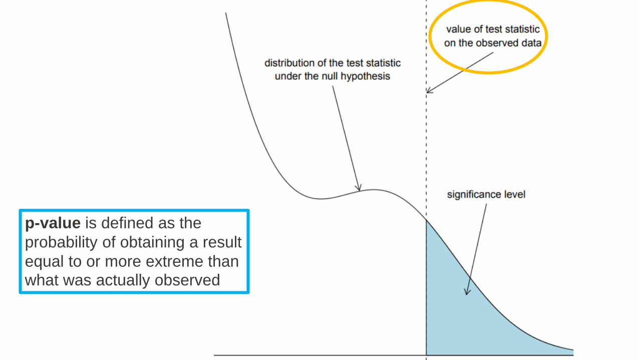
p-value is defined as the
probability of obtaining a result
equal to or more extreme than what was actually observed
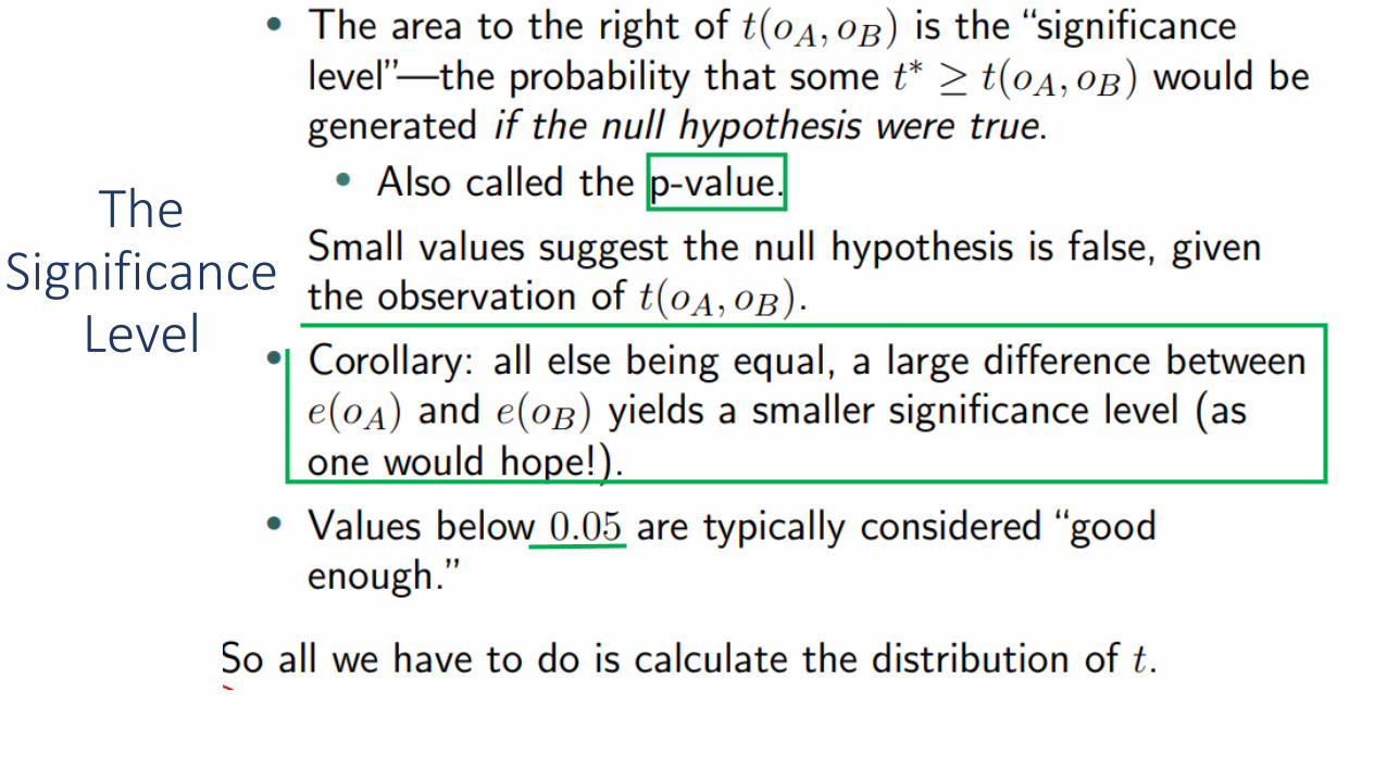
The Significance
Level
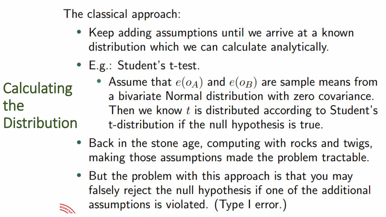
Calculating the Distribution
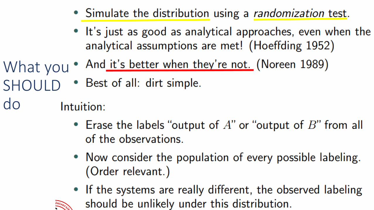
What you SHOULD do
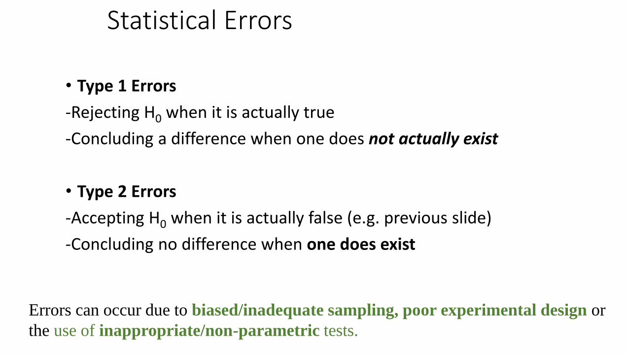
Statistical Errors
• Type 1 Errors
-Rejecting H0 when it is actually true
-Concluding a difference when one does not actually exist
• Type 2 Errors
-Accepting H0 when it is actually false (e.g. previous slide)
-Concluding no difference when one does exist
Errors can occur due to biased/inadequate sampling, poor experimental design or
the use of inappropriate/non-parametric tests.
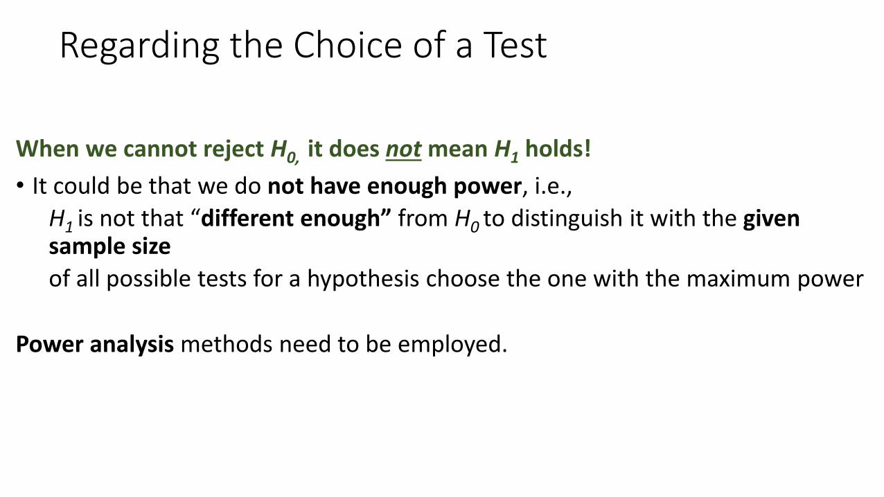
Regarding the Choice of a Test
When we cannot reject H0, it does not mean H1 holds!
• It could be that we do not have enough power, i.e.,
H1 is not that “different enough” from H0 to distinguish it with the given sample size
of all possible tests for a hypothesis choose the one with the maximum power
Power analysis methods need to be employed.


CS – 590.21 Analysis and Modeling of Brain NetworksDepartment of Computer Science
University of Crete
Lecture on Modeling Tools for Assessing Temporal Correlation
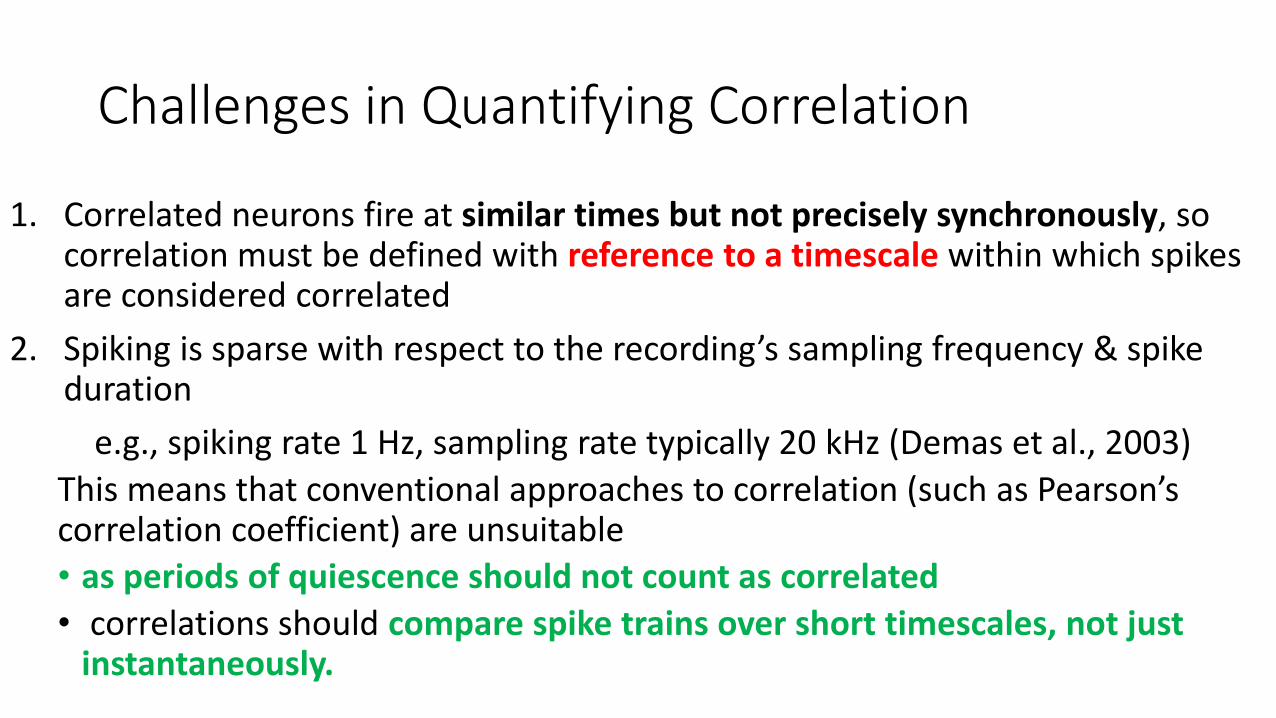
Challenges in Quantifying Correlation
1. Correlated neurons fire at similar times but not precisely synchronously, so correlation must be defined with reference to a timescale within which spikes are considered correlated
2. Spiking is sparse with respect to the recording’s sampling frequency & spike duration
e.g., spiking rate 1 Hz, sampling rate typically 20 kHz (Demas et al., 2003)
This means that conventional approaches to correlation (such as Pearson’s correlation coefficient) are unsuitable
• as periods of quiescence should not count as correlated
• correlations should compare spike trains over short timescales, not just instantaneously.
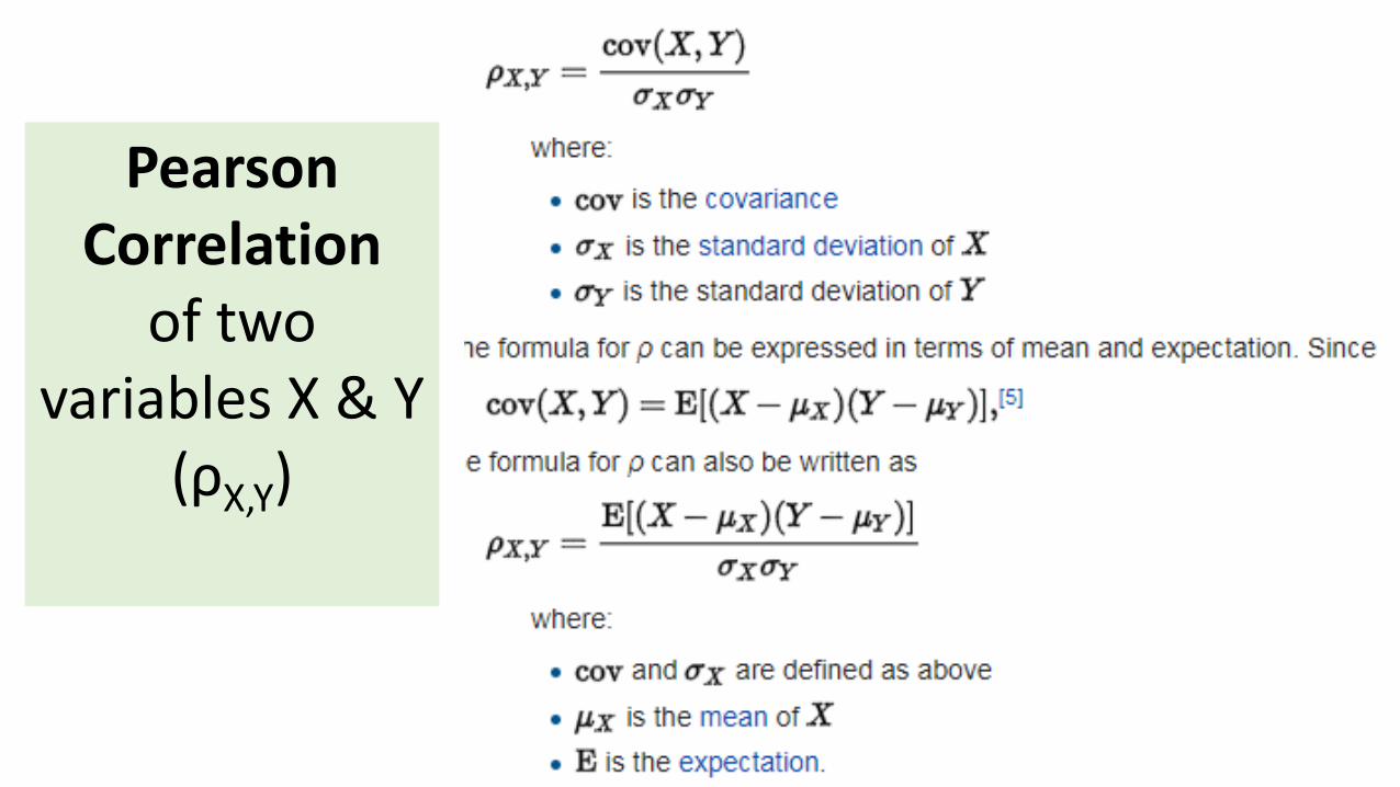
Pearson Correlation
of two variables X & Y
(ρΧ,Υ)
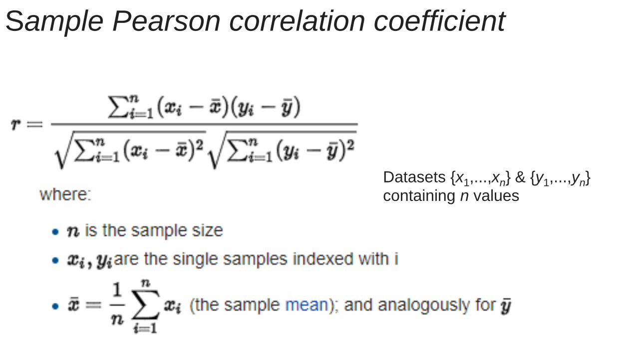
Sample Pearson correlation coefficient
Datasets {x1,...,xn} & {y1,...,yn} containing n values
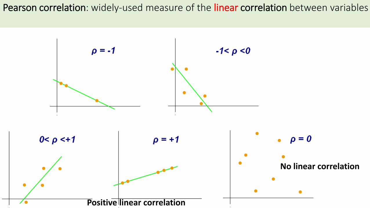
Pearson correlation: widely-used measure of the linear correlation between variables
No linear correlation
Positive linear correlation
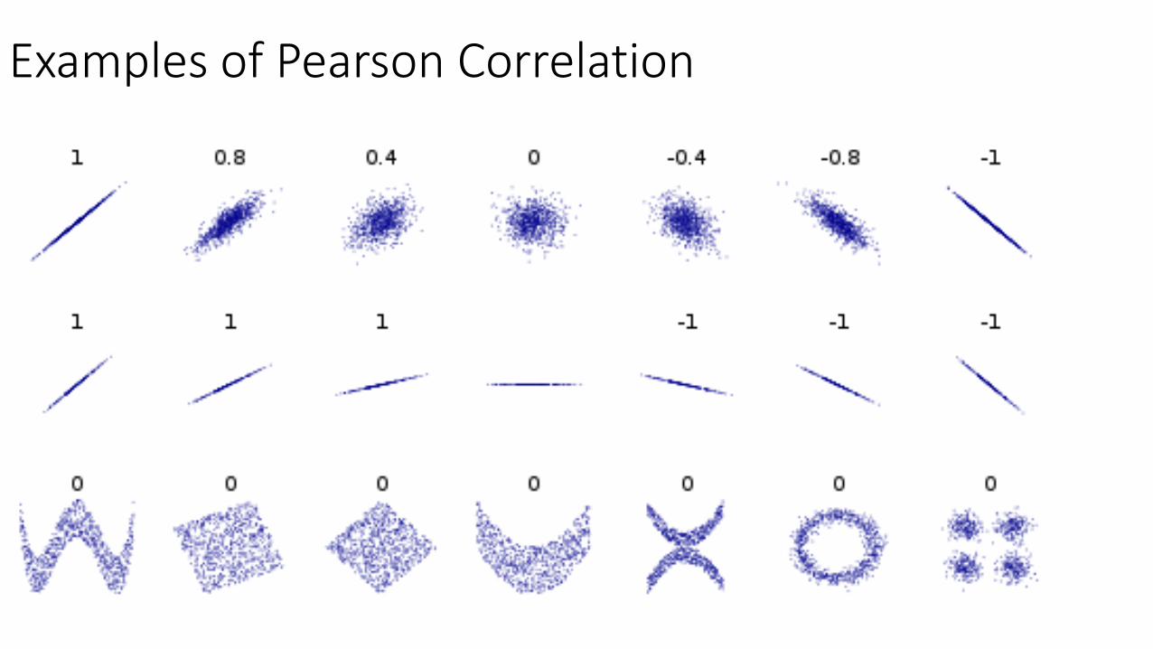
Examples of Pearson Correlation
Quantification of Correlation between Neural Spike Trains
• Key part of the analysis of experimental data
• Neural coordination is thought to play a key role in
• information propagation & processing
• self-organization of the neural system during development
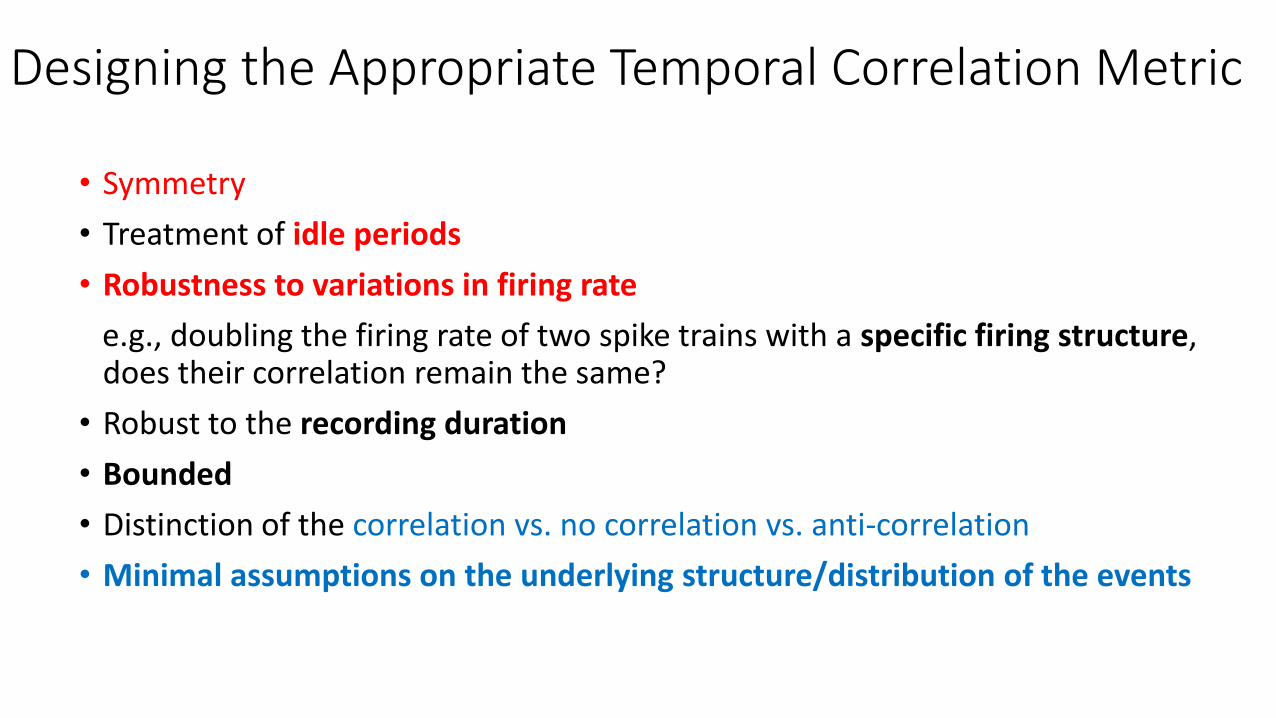
Designing the Appropriate Temporal Correlation Metric
• Symmetry
• Treatment of idle periods
• Robustness to variations in firing rate
e.g., doubling the firing rate of two spike trains with a specific firing structure, does their correlation remain the same?
• Robust to the recording duration
• Bounded
• Distinction of the correlation vs. no correlation vs. anti-correlation
• Minimal assumptions on the underlying structure/distribution of the events
Directional STTC Temporal Correlation Metric
Extended STTC metric to take into consideration the temporal order of the correlation of the spike trains of two neurons
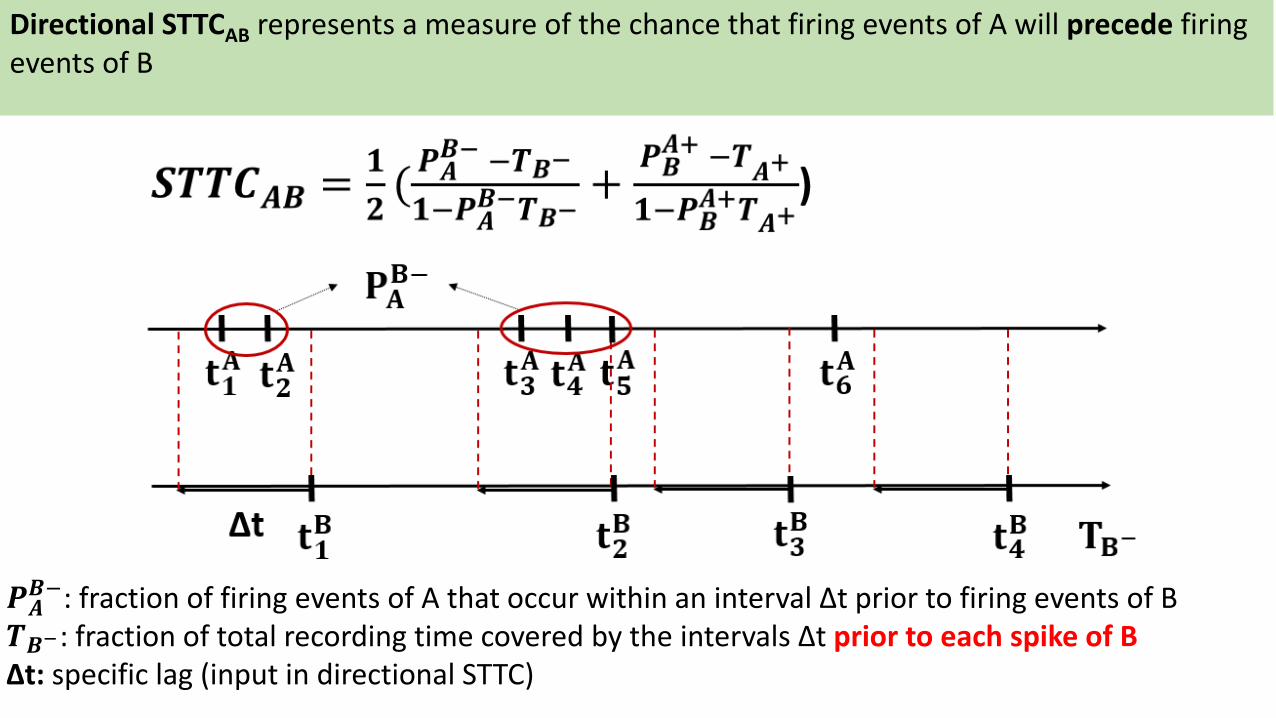
𝑷𝑨𝑩−: fraction of firing events of A that occur within an interval Δt prior to firing events of B
𝑻𝑩−: fraction of total recording time covered by the intervals Δt prior to each spike of BΔt: specific lag (input in directional STTC)
Directional STTCAB represents a measure of the chance that firing events of A will precede firing events of B
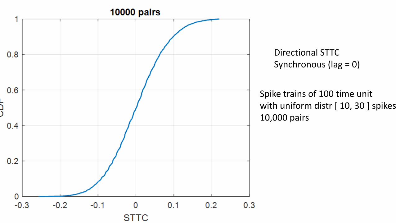
Directional STTC Synchronous (lag = 0)
Spike trains of 100 time unitwith uniform distr [ 10, 30 ] spikes10,000 pairs
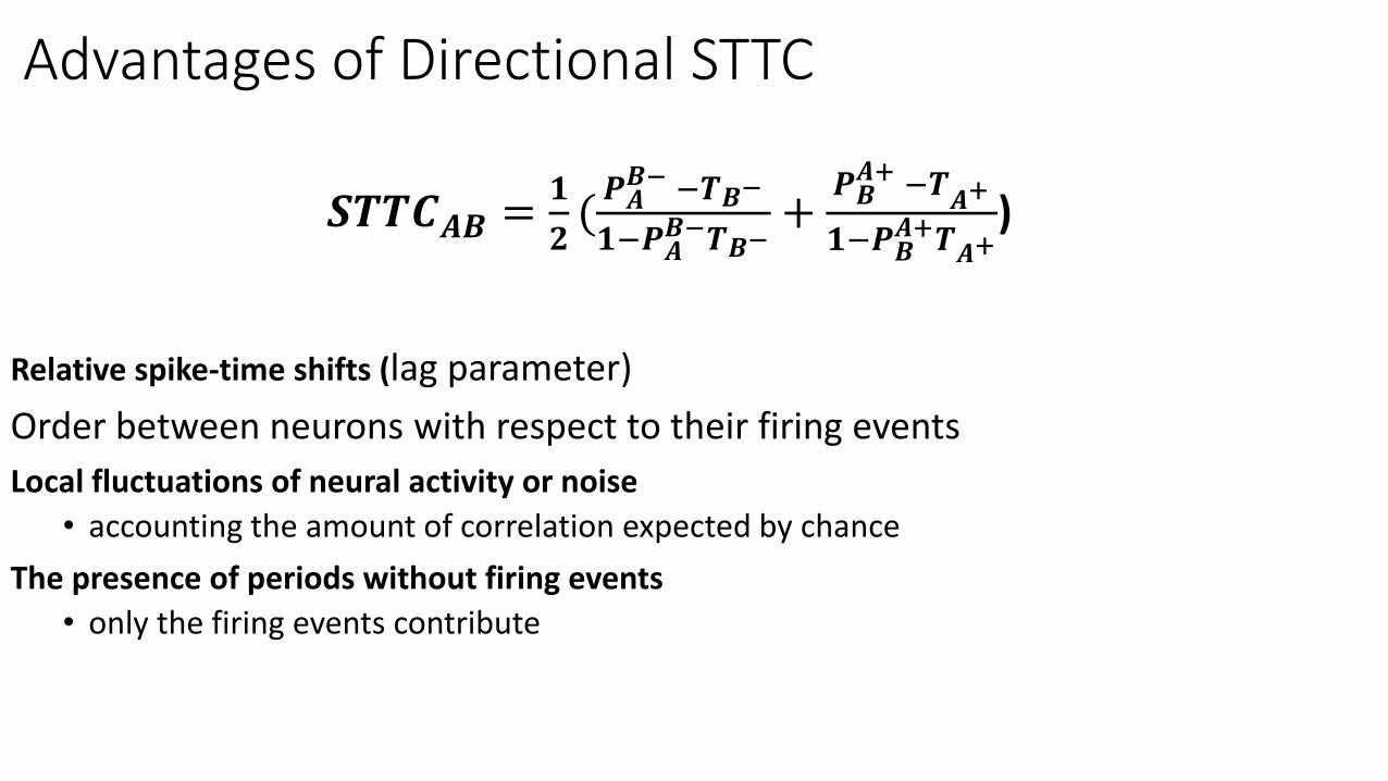
Advantages of Directional STTC
Relative spike-time shifts (lag parameter)
Order between neurons with respect to their firing events
Local fluctuations of neural activity or noise
• accounting the amount of correlation expected by chance
The presence of periods without firing events
• only the firing events contribute
𝑺𝑻𝑻𝑪𝑨𝑩 =𝟏
𝟐(𝑷𝑨𝑩− −𝑻𝑩−
𝟏−𝑷𝑨𝑩−𝑻𝑩−
+𝑷𝑩𝑨+ −𝑻
𝑨+
𝟏−𝑷𝑩𝑨+𝑻𝑨+
)
CA
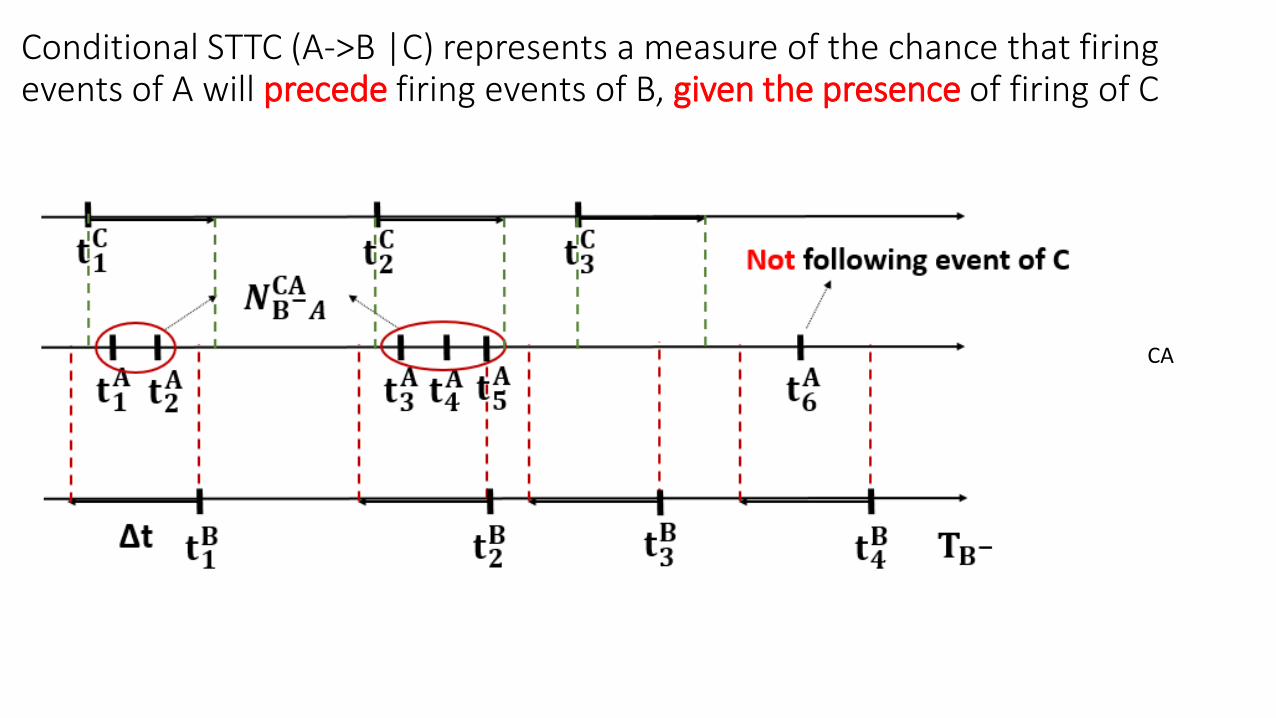
Conditional STTC (A->B |C) represents a measure of the chance that firing events of A will precede firing events of B, given the presence of firing of C
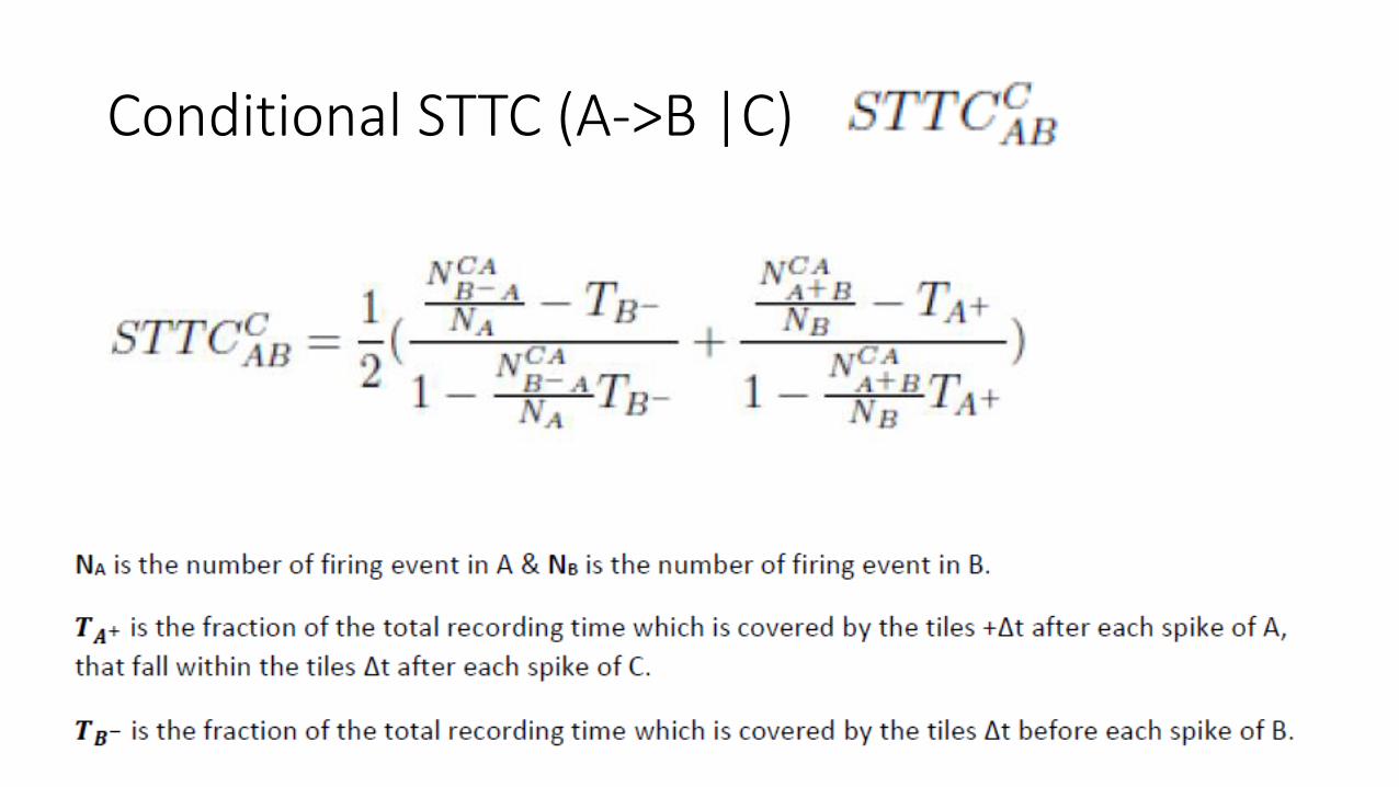
Conditional STTC (A->B |C)
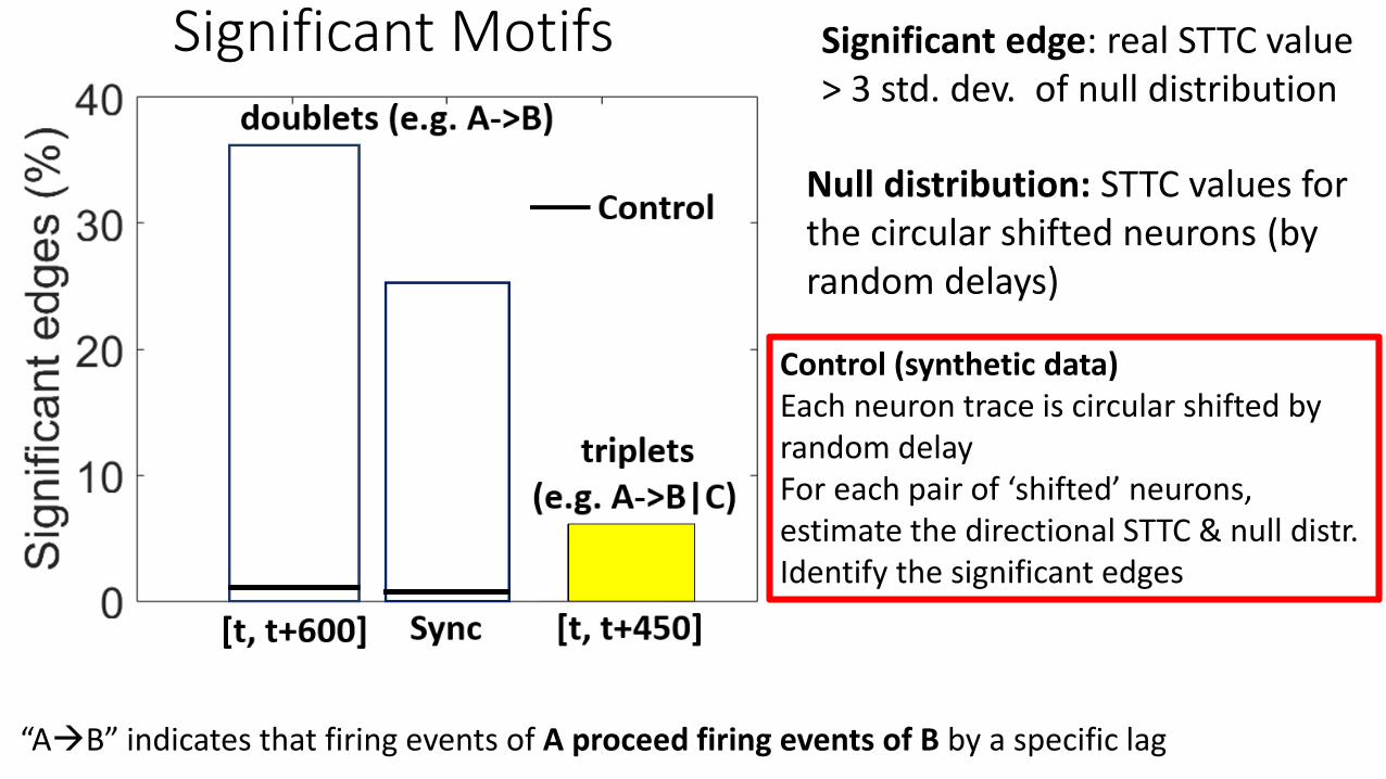
“AB” indicates that firing events of A proceed firing events of B by a specific lag
Null distribution: STTC values for the circular shifted neurons (by random delays)
Significant Motifs Significant edge: real STTC value > 3 std. dev. of null distribution
Control (synthetic data)Each neuron trace is circular shifted by random delayFor each pair of ‘shifted’ neurons, estimate the directional STTC & null distr.Identify the significant edges
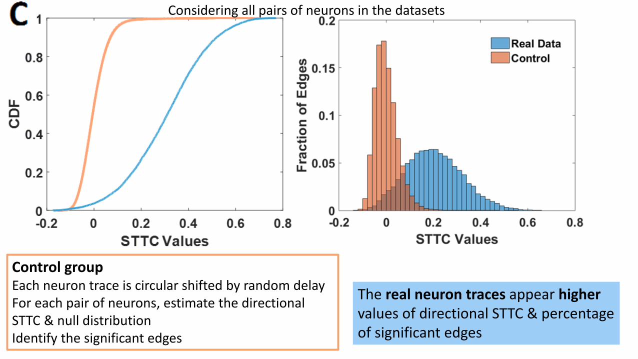
Control groupEach neuron trace is circular shifted by random delayFor each pair of neurons, estimate the directional STTC & null distributionIdentify the significant edges
The real neuron traces appear highervalues of directional STTC & percentage of significant edges
Considering all pairs of neurons in the datasets
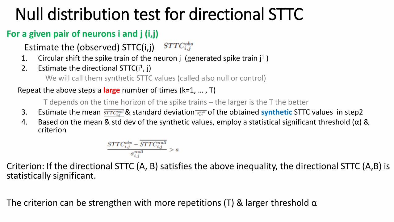
Null distribution test for directional STTC For a given pair of neurons i and j (i,j)
Estimate the (observed) STTC(i,j)1. Circular shift the spike train of the neuron j (generated spike train j1 )2. Estimate the directional STTC(i1, j)
We will call them synthetic STTC values (called also null or control)
Repeat the above steps a large number of times (k=1, … , T)
T depends on the time horizon of the spike trains – the larger is the T the better3. Estimate the mean & standard deviation of the obtained synthetic STTC values in step24. Based on the mean & std dev of the synthetic values, employ a statistical significant threshold (α) &
criterion
Criterion: If the directional STTC (A, B) satisfies the above inequality, the directional STTC (A,B) is statistically significant.
The criterion can be strengthen with more repetitions (T) & larger threshold α
Strengthen the Criterion of Significant Directional STTC (A,B)
Additional requirements
• The total number of spikes of A within a STTC lag of spikes of B is above 3.
• The total number of spikes of B within a STTC lag of spikes of A is above 3.
Kolmogorov-Smirnov (K-S) Test
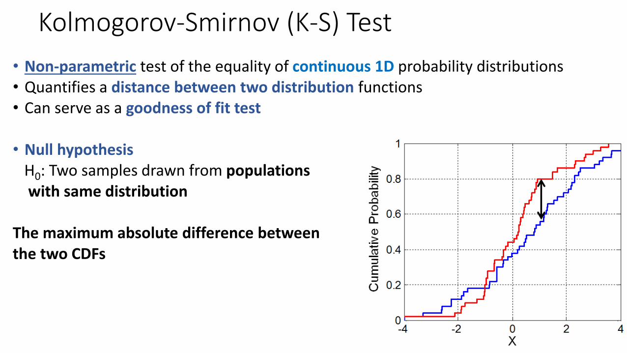
• Non-parametric test of the equality of continuous 1D probability distributions• Quantifies a distance between two distribution functions• Can serve as a goodness of fit test
• Null hypothesisH0: Two samples drawn from populations with same distribution
The maximum absolute difference betweenthe two CDFs
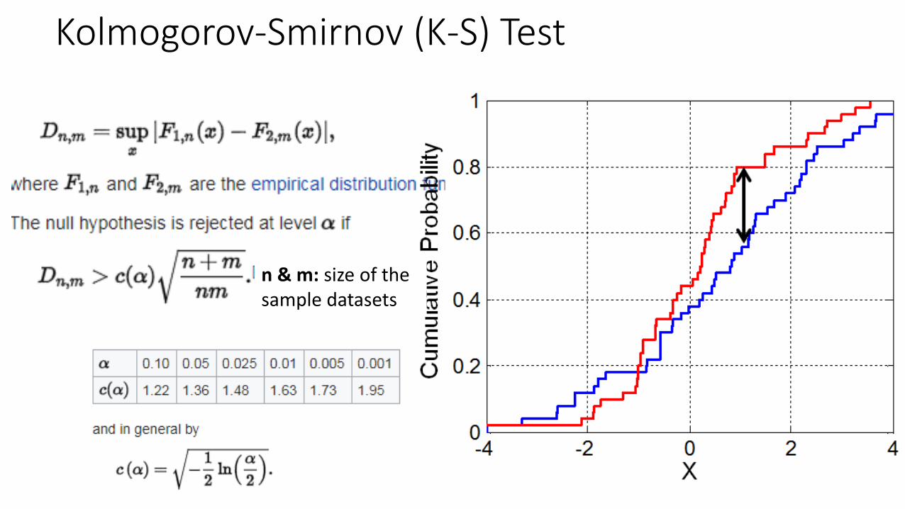
Kolmogorov-Smirnov (K-S) Test
n & m: size of the sample datasets
Kolmogorov-Smirnov (K-S) Test
Kolmogorov computed the expected distribution of the distance of the two CDFs when the null hypothesis is true.
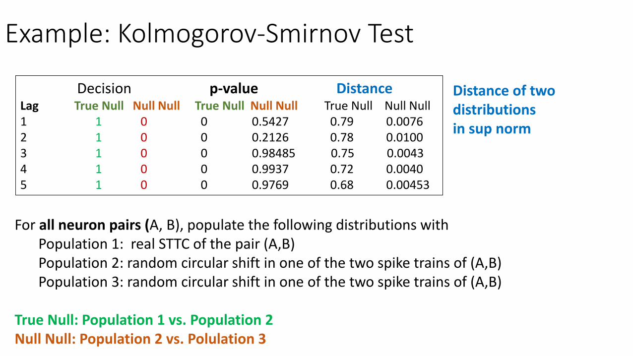
Example: Kolmogorov-Smirnov Test
Decision p-value DistanceLag True Null Null Null True Null Null Null True Null Null Null1 1 0 0 0.5427 0.79 0.00762 1 0 0 0.2126 0.78 0.01003 1 0 0 0.98485 0.75 0.00434 1 0 0 0.9937 0.72 0.00405 1 0 0 0.9769 0.68 0.00453
For all neuron pairs (A, B), populate the following distributions withPopulation 1: real STTC of the pair (A,B)Population 2: random circular shift in one of the two spike trains of (A,B)Population 3: random circular shift in one of the two spike trains of (A,B)
True Null: Population 1 vs. Population 2Null Null: Population 2 vs. Polulation 3
Distance of two distributionsin sup norm
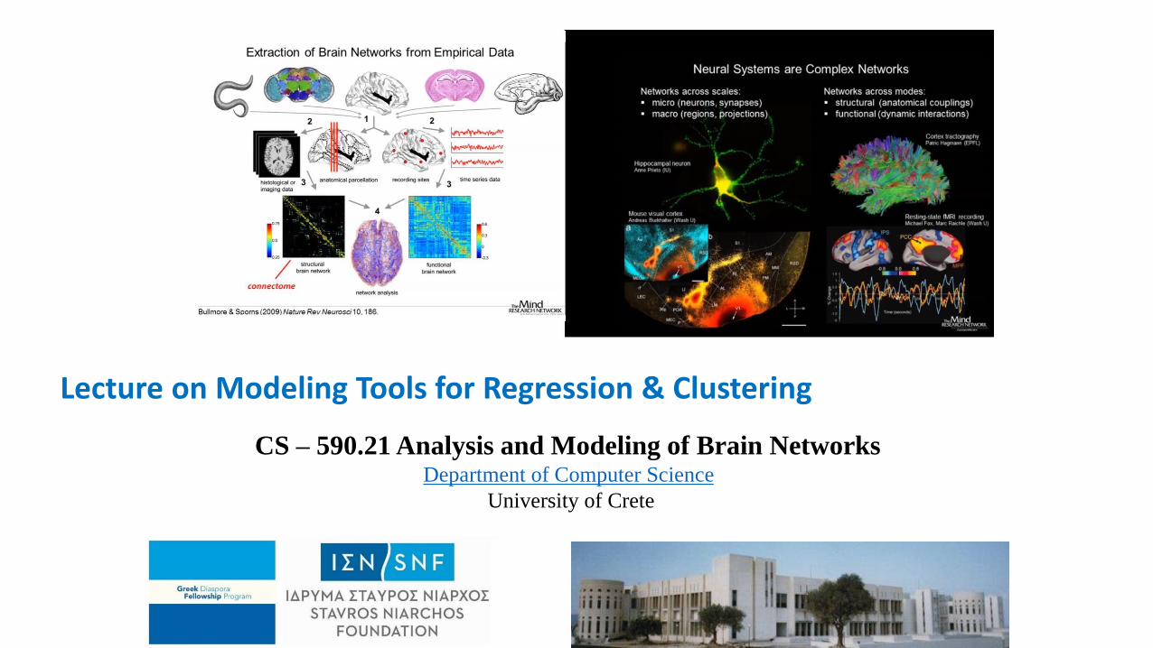
CS – 590.21 Analysis and Modeling of Brain NetworksDepartment of Computer Science
University of Crete
Lecture on Modeling Tools for Regression & Clustering

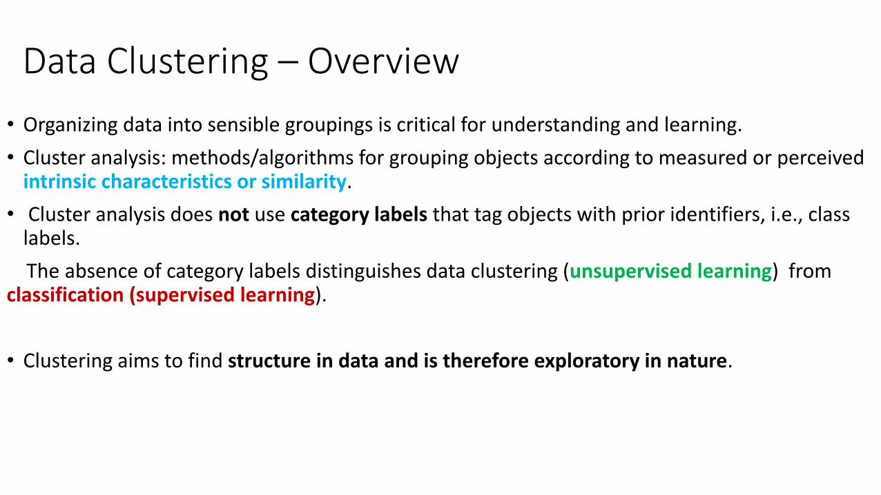
Data Clustering – Overview
• Organizing data into sensible groupings is critical for understanding and learning.
• Cluster analysis: methods/algorithms for grouping objects according to measured or perceived intrinsic characteristics or similarity.
• Cluster analysis does not use category labels that tag objects with prior identifiers, i.e., class labels.
The absence of category labels distinguishes data clustering (unsupervised learning) from classification (supervised learning).
• Clustering aims to find structure in data and is therefore exploratory in nature.
• Clustering has a long rich history in various scientific fields.
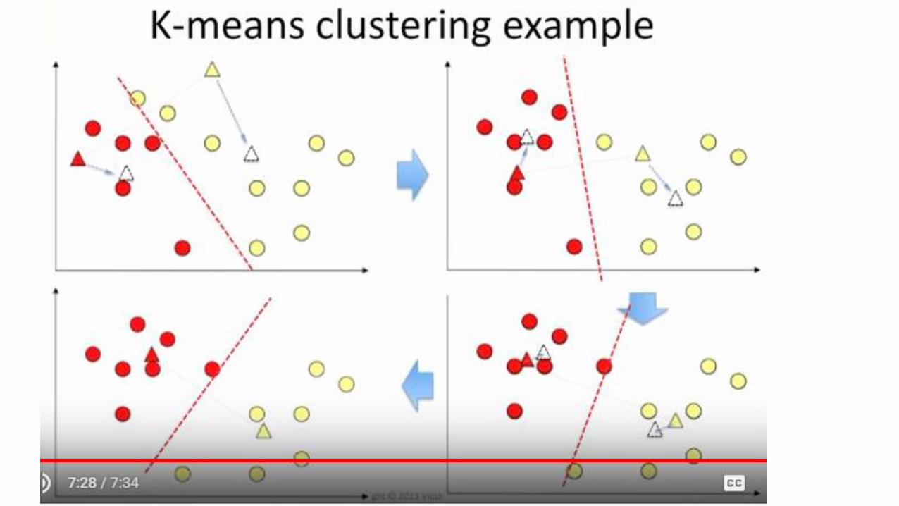
K-means (1955): One of the most popular simple clustering algorithms
Still widely-used.
The design of a general purpose clustering algorithm is a difficult task
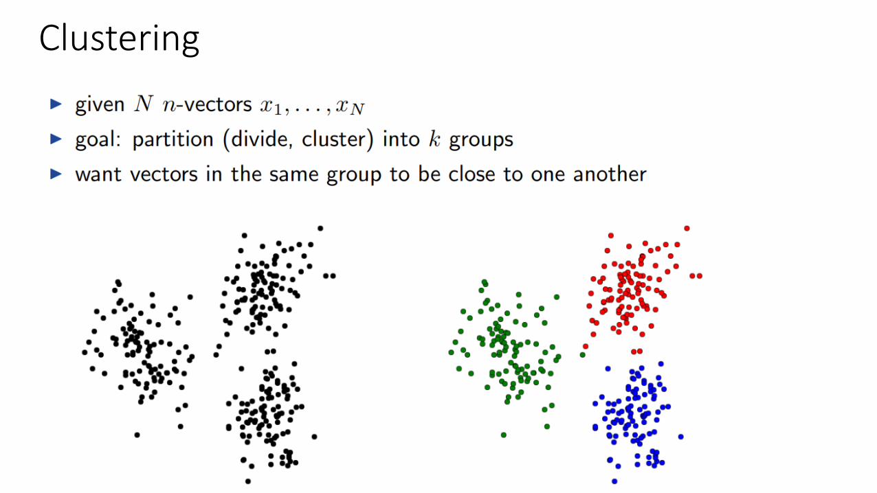
Clustering
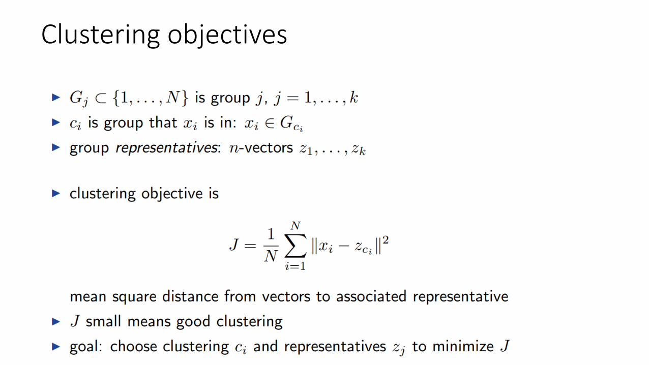
Clustering objectives
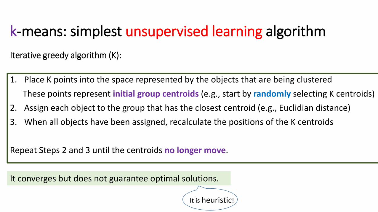
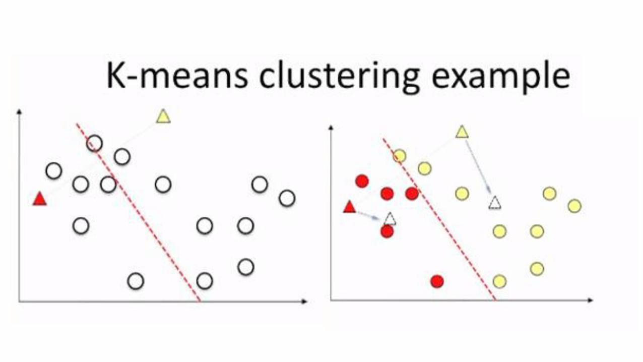
k-means: simplest unsupervised learning algorithm
Iterative greedy algorithm (K):
1. Place K points into the space represented by the objects that are being clustered
These points represent initial group centroids (e.g., start by randomly selecting K centroids)
2. Assign each object to the group that has the closest centroid (e.g., Euclidian distance)
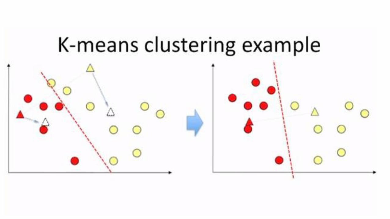
3. When all objects have been assigned, recalculate the positions of the K centroids
Repeat Steps 2 and 3 until the centroids no longer move.
It converges but does not guarantee optimal solutions.
It is heuristic!
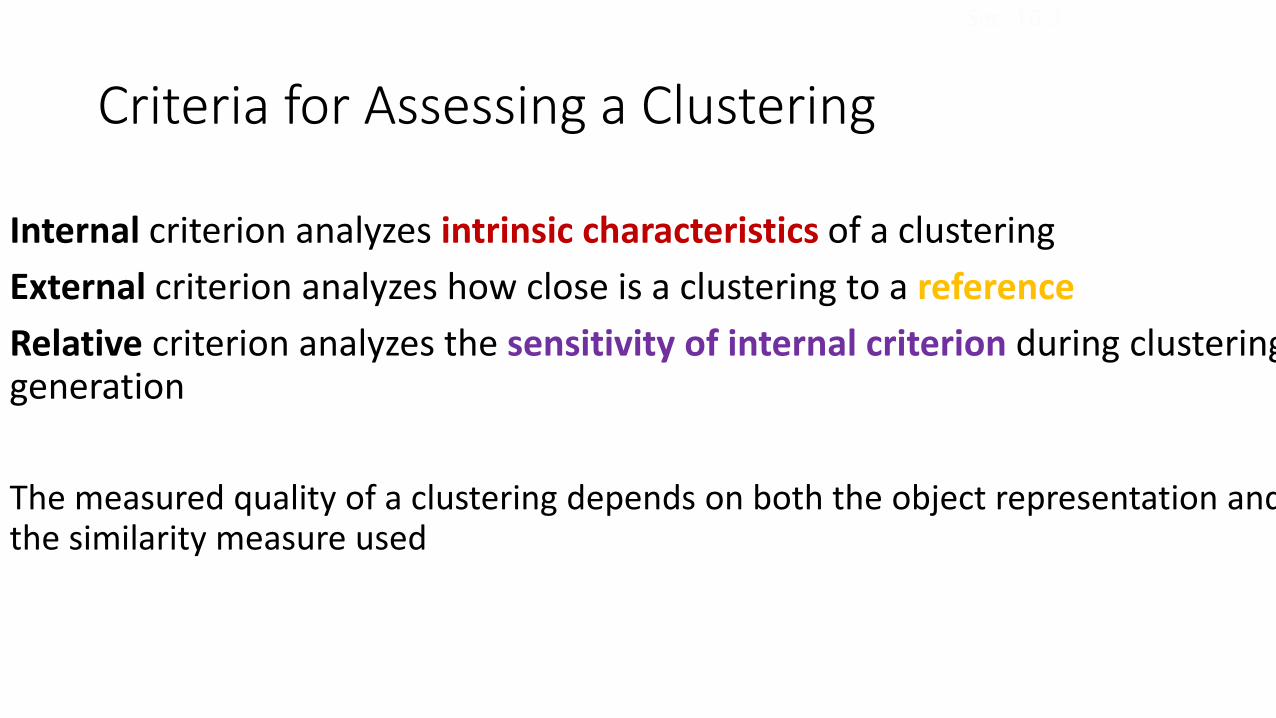
Criteria for Assessing a Clustering
Internal criterion analyzes intrinsic characteristics of a clustering
External criterion analyzes how close is a clustering to a reference
Relative criterion analyzes the sensitivity of internal criterion during clustering generation
The measured quality of a clustering depends on both the object representation and the similarity measure used
Sec. 16.3
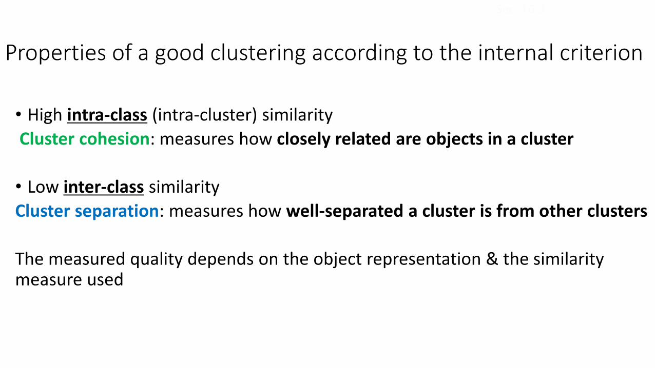
Properties of a good clustering according to the internal criterion
• High intra-class (intra-cluster) similarity
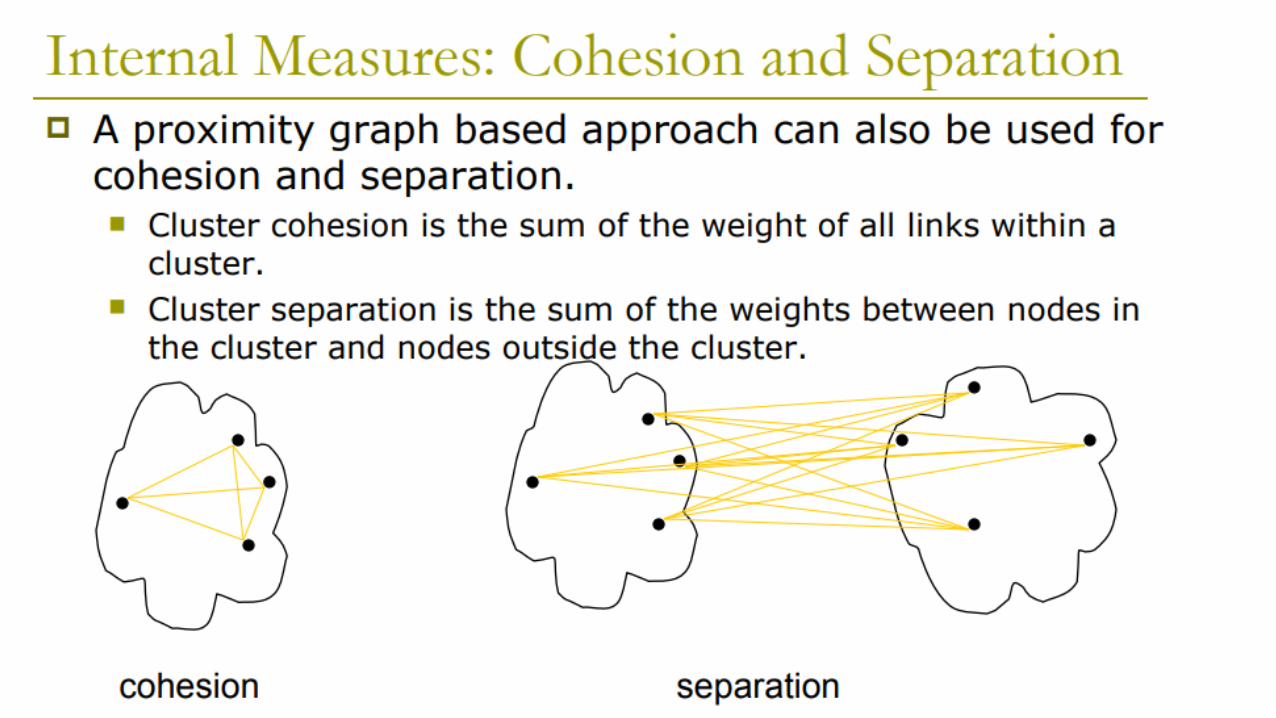
Cluster cohesion: measures how closely related are objects in a cluster
• Low inter-class similarity
Cluster separation: measures how well-separated a cluster is from other clusters
The measured quality depends on the object representation & the similarity measure used
Sec. 16.3
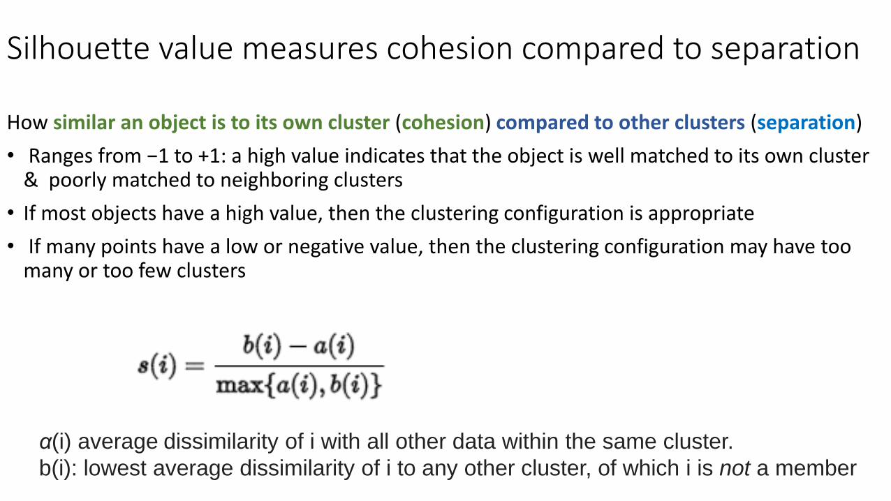
Silhouette value measures cohesion compared to separation
How similar an object is to its own cluster (cohesion) compared to other clusters (separation)
• Ranges from −1 to +1: a high value indicates that the object is well matched to its own cluster & poorly matched to neighboring clusters
• If most objects have a high value, then the clustering configuration is appropriate
• If many points have a low or negative value, then the clustering configuration may have too many or too few clusters
α(i) average dissimilarity of i with all other data within the same cluster.
b(i): lowest average dissimilarity of i to any other cluster, of which i is not a member
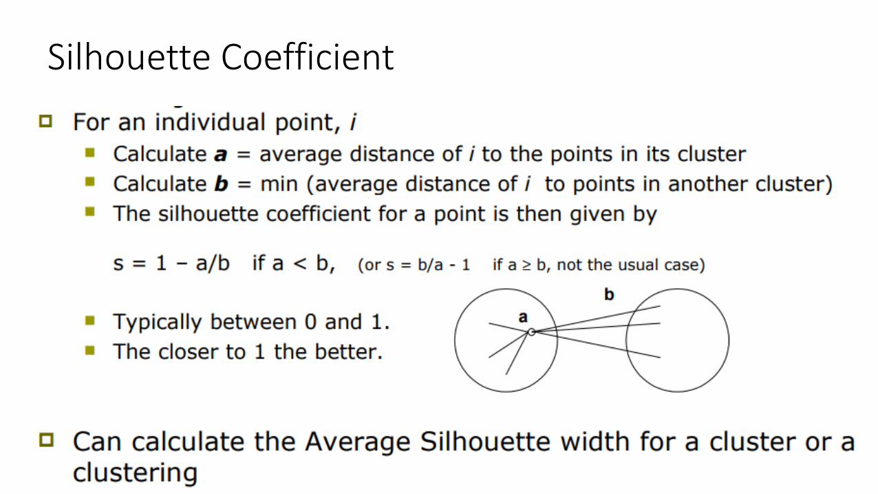
Silhouette Coefficient
External criteria for clustering quality
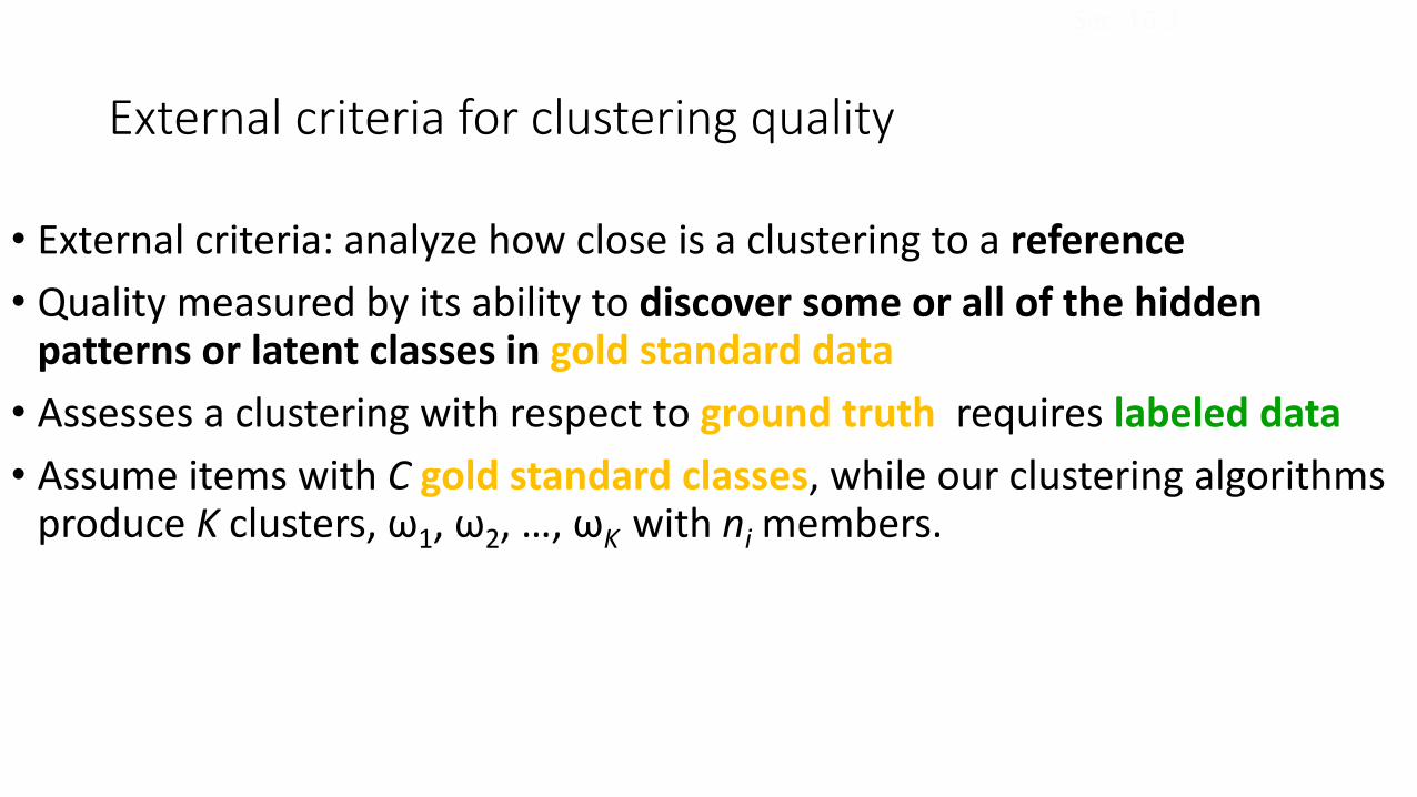
• External criteria: analyze how close is a clustering to a reference
• Quality measured by its ability to discover some or all of the hidden patterns or latent classes in gold standard data
• Assesses a clustering with respect to ground truth requires labeled data
• Assume items with C gold standard classes, while our clustering algorithms produce K clusters, ω1, ω2, …, ωK with ni members.
Sec. 16.3
External Evaluation of Cluster Quality (cont’d)
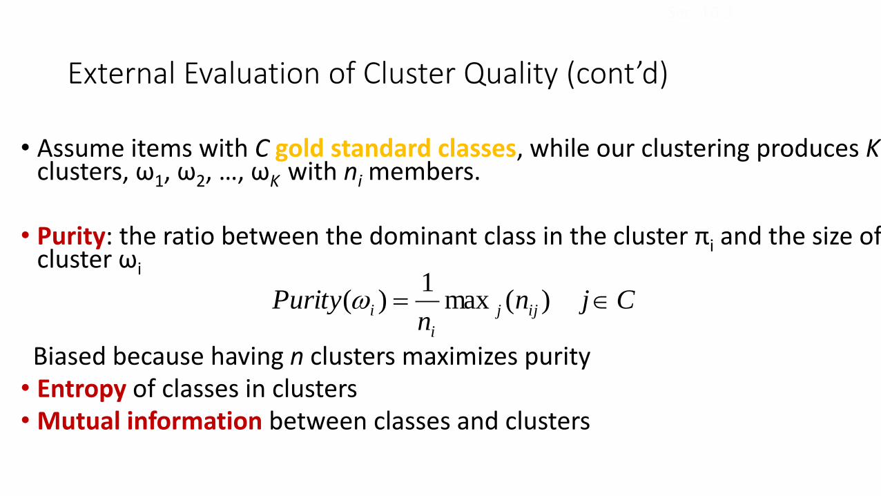
• Assume items with C gold standard classes, while our clustering produces Kclusters, ω1, ω2, …, ωK with ni members.
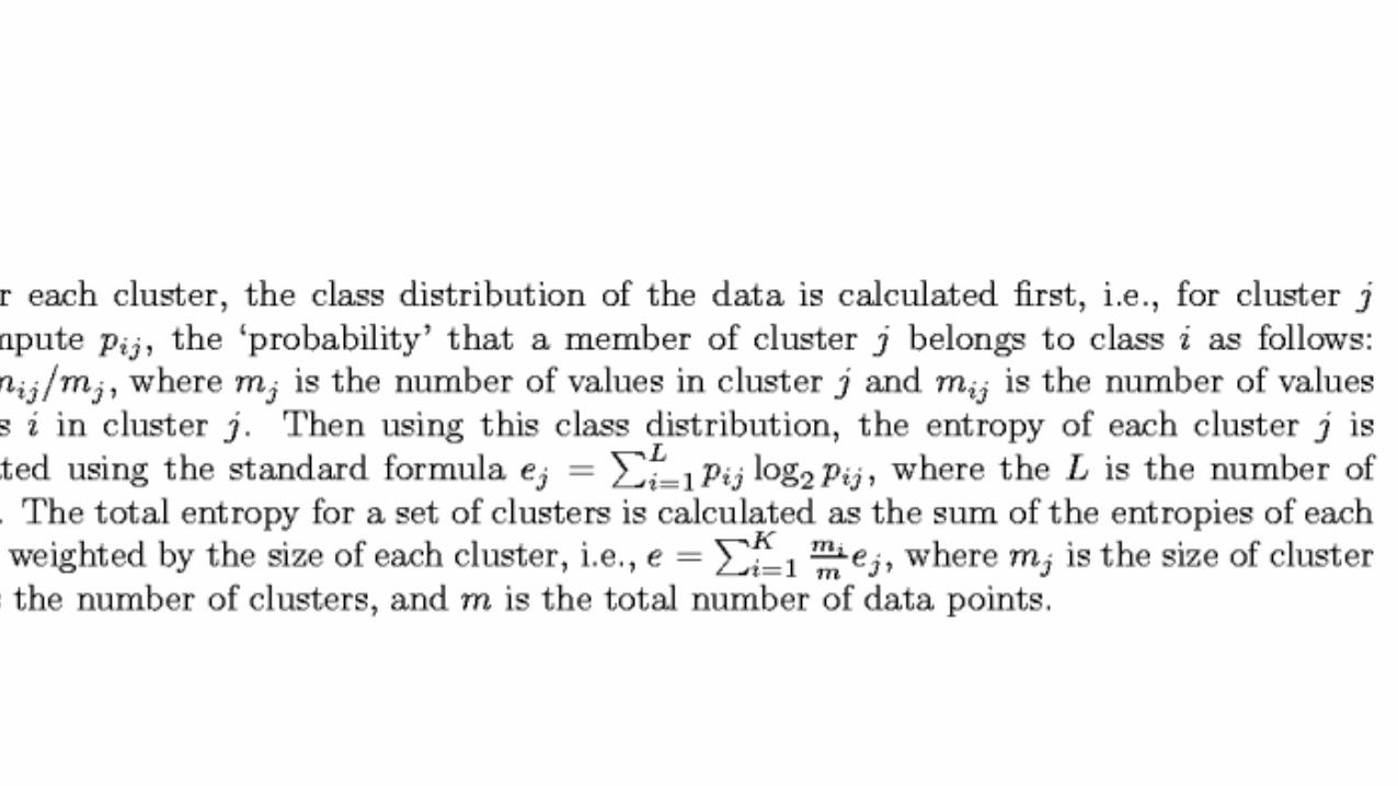
• Purity: the ratio between the dominant class in the cluster πi and the size of cluster ωi
Biased because having n clusters maximizes purity• Entropy of classes in clusters • Mutual information between classes and clusters
Cjnn
Purity ijj
i
i )(max1
)(
Sec. 16.3
Cluster I Cluster II Cluster III
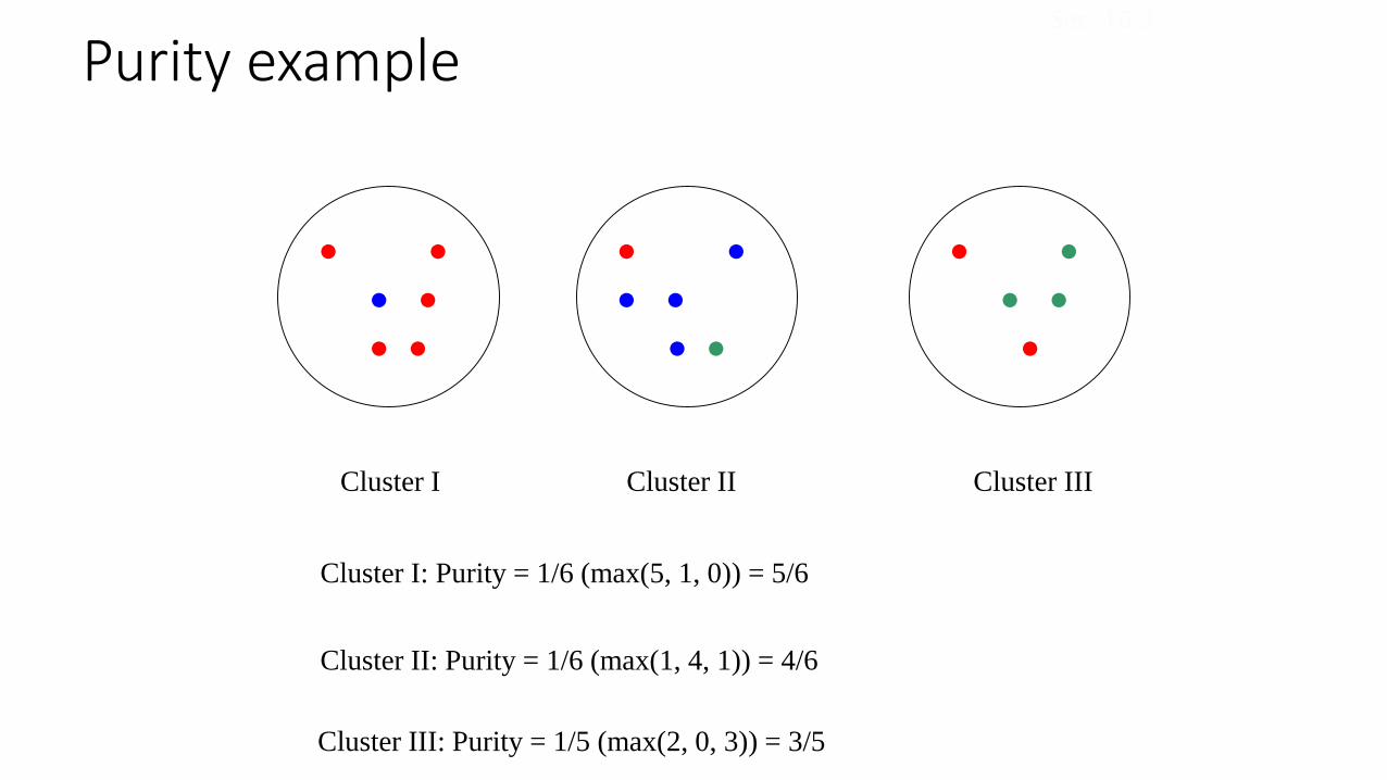
Cluster I: Purity = 1/6 (max(5, 1, 0)) = 5/6
Cluster II: Purity = 1/6 (max(1, 4, 1)) = 4/6
Cluster III: Purity = 1/5 (max(2, 0, 3)) = 3/5
Purity exampleSec. 16.3
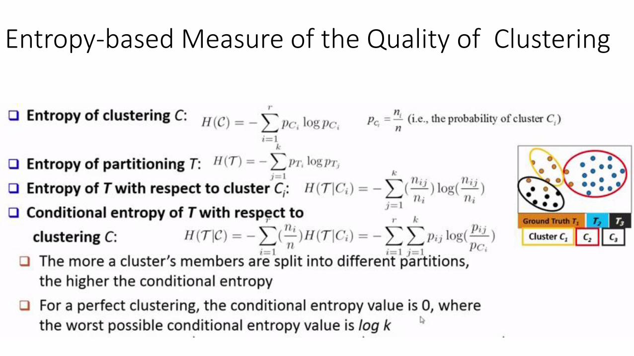
Entropy-based Measure of the Quality of Clustering
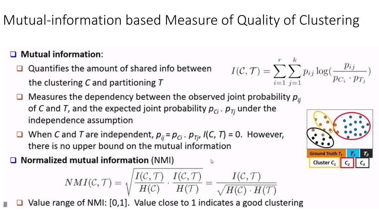
Mutual-information based Measure of Quality of Clustering
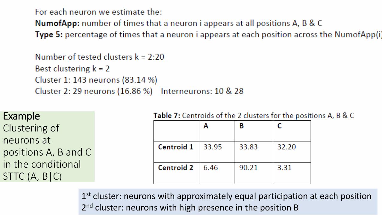
ExampleClustering of neurons at positions A, B and C in the conditional STTC (A, B|C)
1st cluster: neurons with approximately equal participation at each position2nd cluster: neurons with high presence in the position B
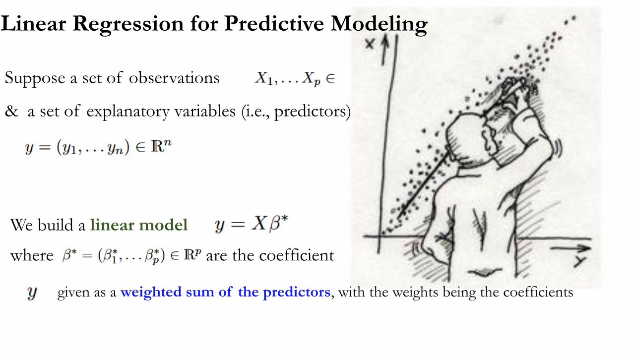
We build a linear model
where are the coefficients of each predictor
Linear Regression for Predictive Modeling
Suppose a set of observations
& a set of explanatory variables (i.e., predictors)
given as a weighted sum of the predictors, with the weights being the coefficients
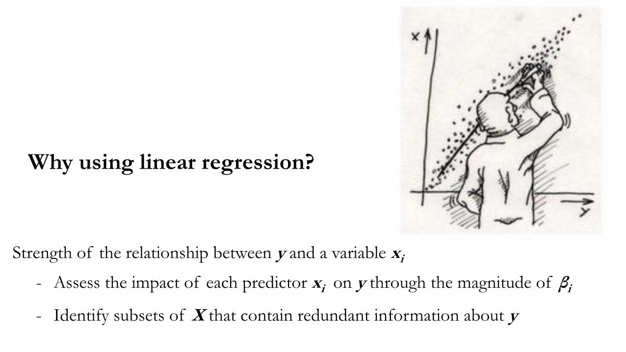
Why using linear regression?
Strength of the relationship between y and a variable xi
- Assess the impact of each predictor xi on y through the magnitude of βi
- Identify subsets of X that contain redundant information about y
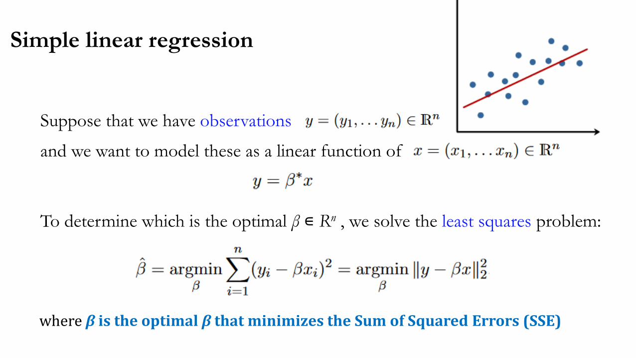
Simple linear regression
Suppose that we have observations
and we want to model these as a linear function of
To determine which is the optimal β ∊ Rn , we solve the least squares problem:
where β is the optimal β that minimizes the Sum of Squared Errors (SSE)
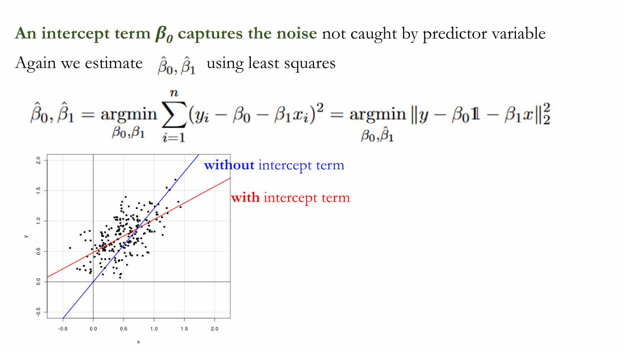
An intercept term β0 captures the noise not caught by predictor variable
Again we estimate using least squares
with intercept term
without intercept term
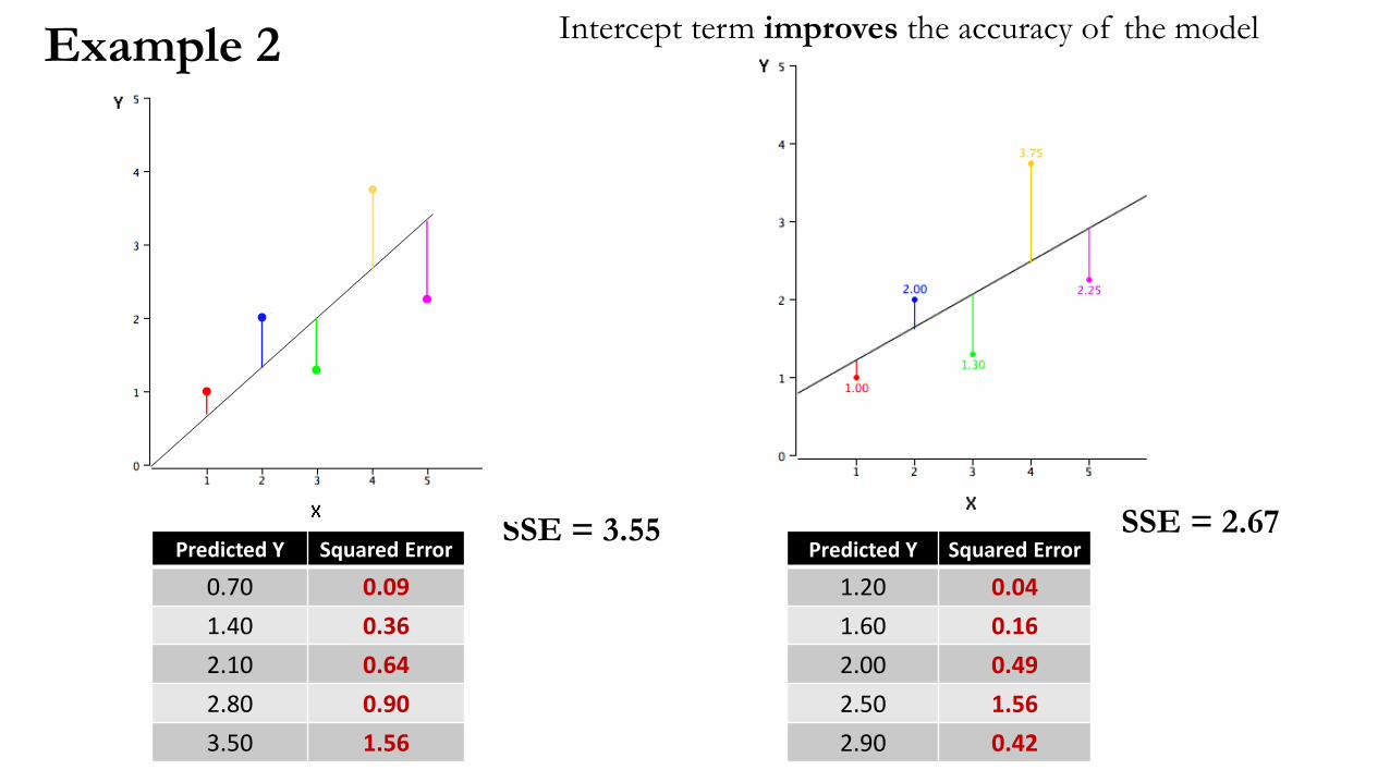
Example 2
Predicted Y Squared Error
0.70 0.09
1.40 0.36
2.10 0.64
2.80 0.90
3.50 1.56
Predicted Y Squared Error
1.20 0.04
1.60 0.16
2.00 0.49
2.50 1.56
2.90 0.42
SSE = 3.55
Intercept term improves the accuracy of the model
SSE = 2.67
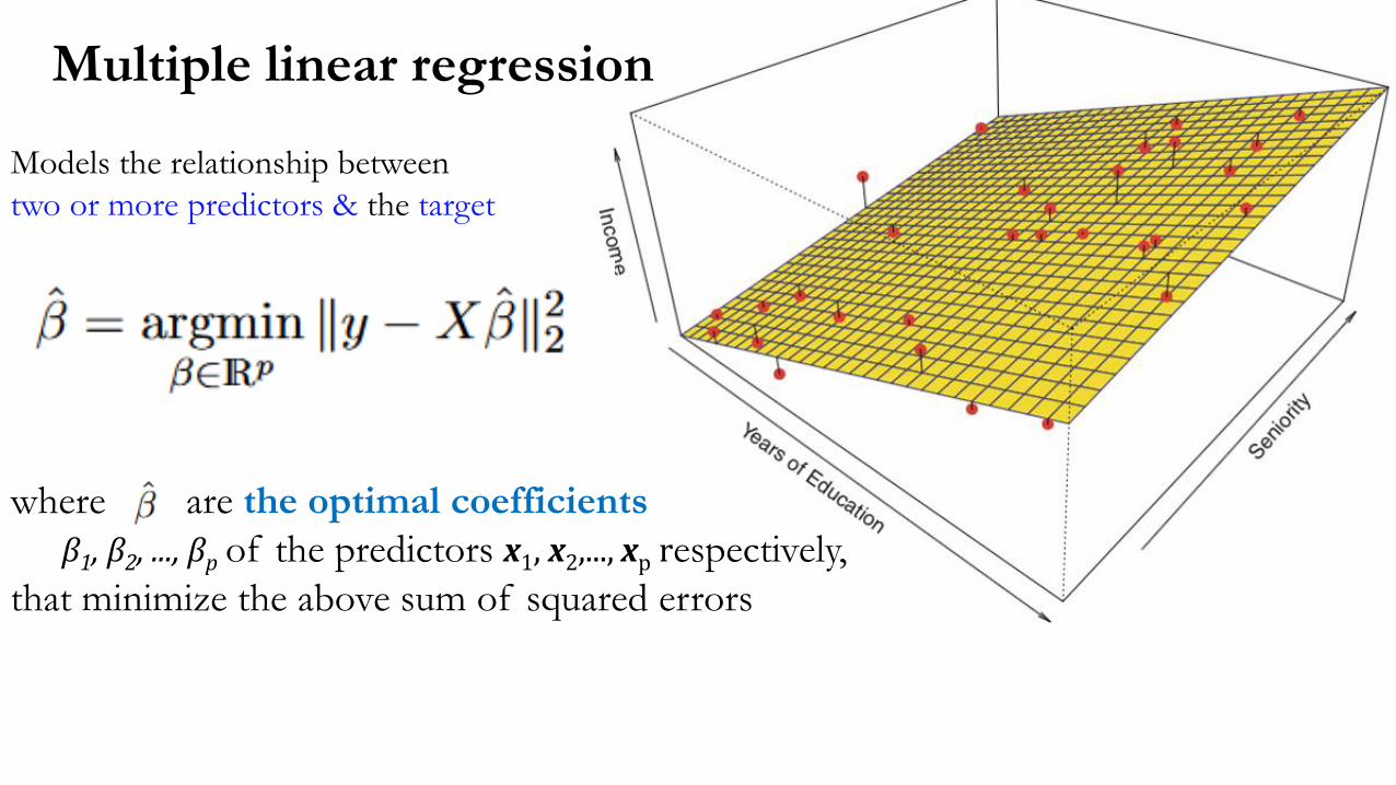
where are the optimal coefficients
β1, β2, ..., βp of the predictors x1, x2,..., xp respectively,
that minimize the above sum of squared errors
Multiple linear regression
Models the relationship between
two or more predictors & the target
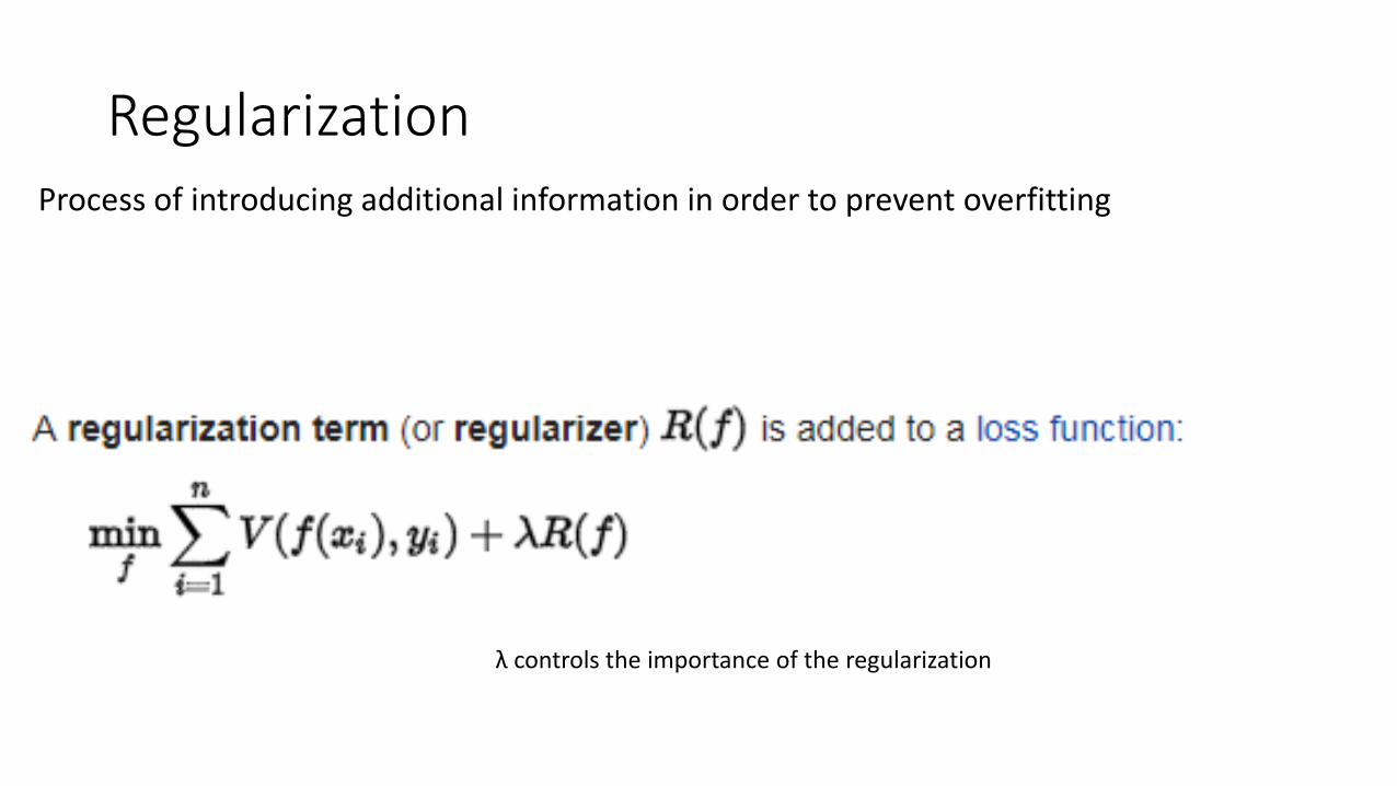
Regularization Process of introducing additional information in order to prevent overfitting
λ controls the importance of the regularization
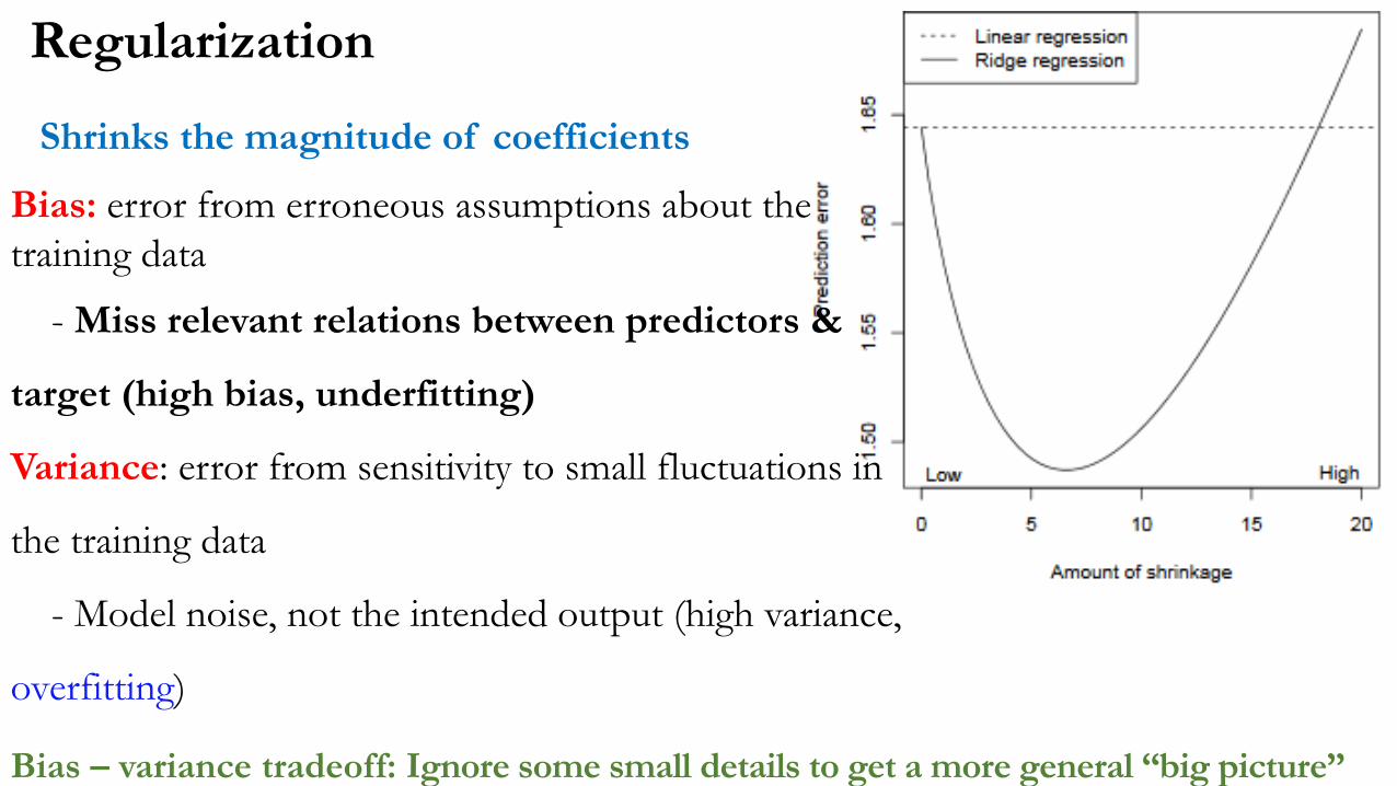
Bias: error from erroneous assumptions about the
training data
- Miss relevant relations between predictors &
target (high bias, underfitting)
Variance: error from sensitivity to small fluctuations in
the training data
- Model noise, not the intended output (high variance,
overfitting)
Bias – variance tradeoff: Ignore some small details to get a more general “big picture”
Regularization
Shrinks the magnitude of coefficients
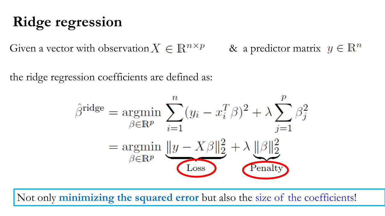
Ridge regression
Given a vector with observations & a predictor matrix
the ridge regression coefficients are defined as:
Not only minimizing the squared error but also the size of the coefficients!
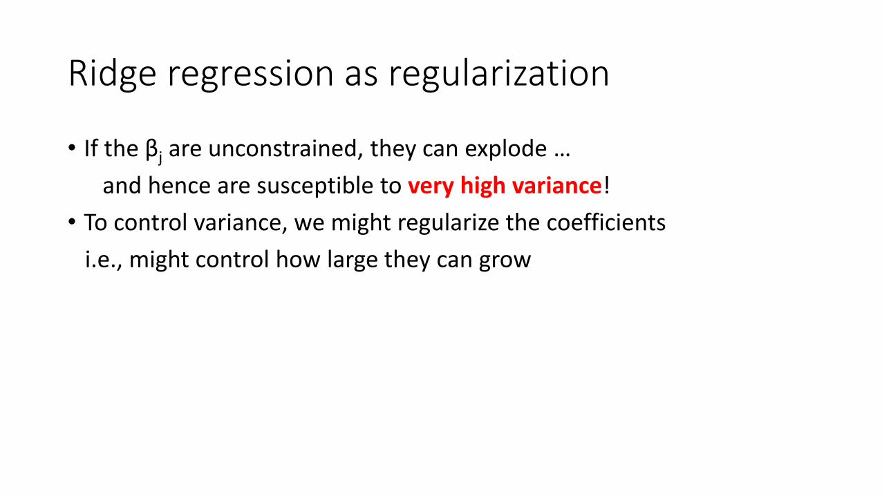
Ridge regression as regularization
• If the βj are unconstrained, they can explode …
and hence are susceptible to very high variance!
• To control variance, we might regularize the coefficients
i.e., might control how large they can grow
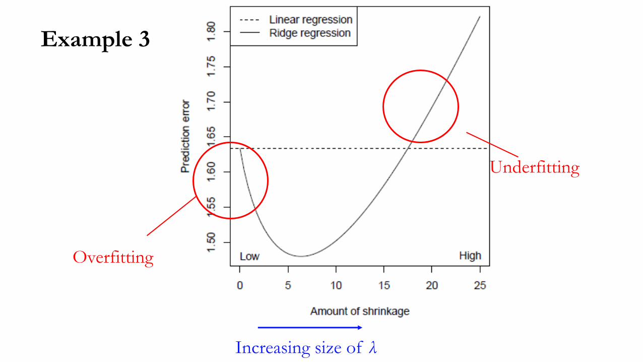
Example 3
Overfitting
Underfitting
Increasing size of λ
In linear model setting, this means estimating some coefficients to be exactly zero
Problem of selecting the most relevant predictors from a larger set of predictors
Variable selection
This can be very important for the purposes of model interpretation
Ridge regression cannot perform variable selection
- Does not set coefficients exactly to zero, unless λ = ∞
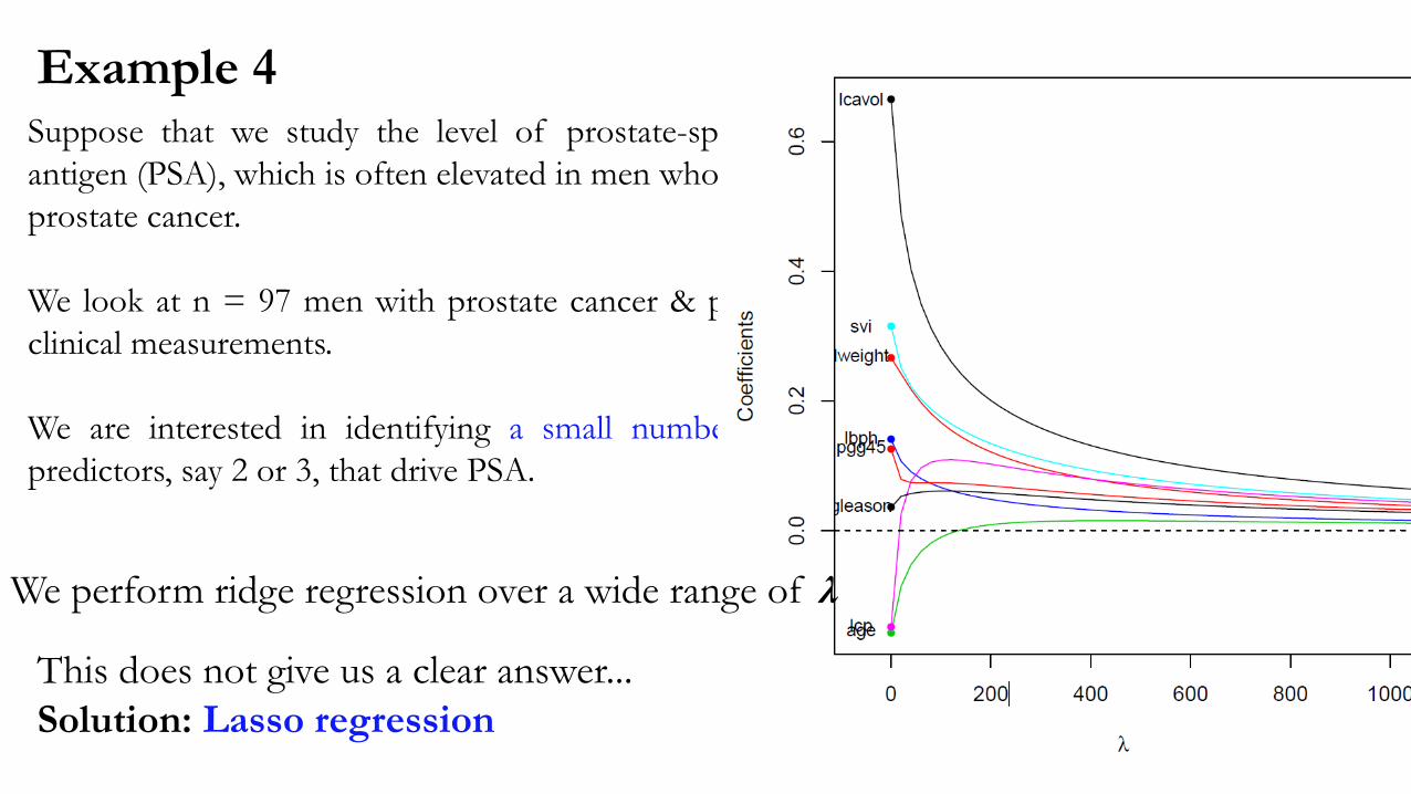
Example 4Suppose that we study the level of prostate-specific
antigen (PSA), which is often elevated in men who have
prostate cancer.
We look at n = 97 men with prostate cancer & p = 8
clinical measurements.
We are interested in identifying a small number of
predictors, say 2 or 3, that drive PSA.
We perform ridge regression over a wide range of λ
This does not give us a clear answer...
Solution: Lasso regression
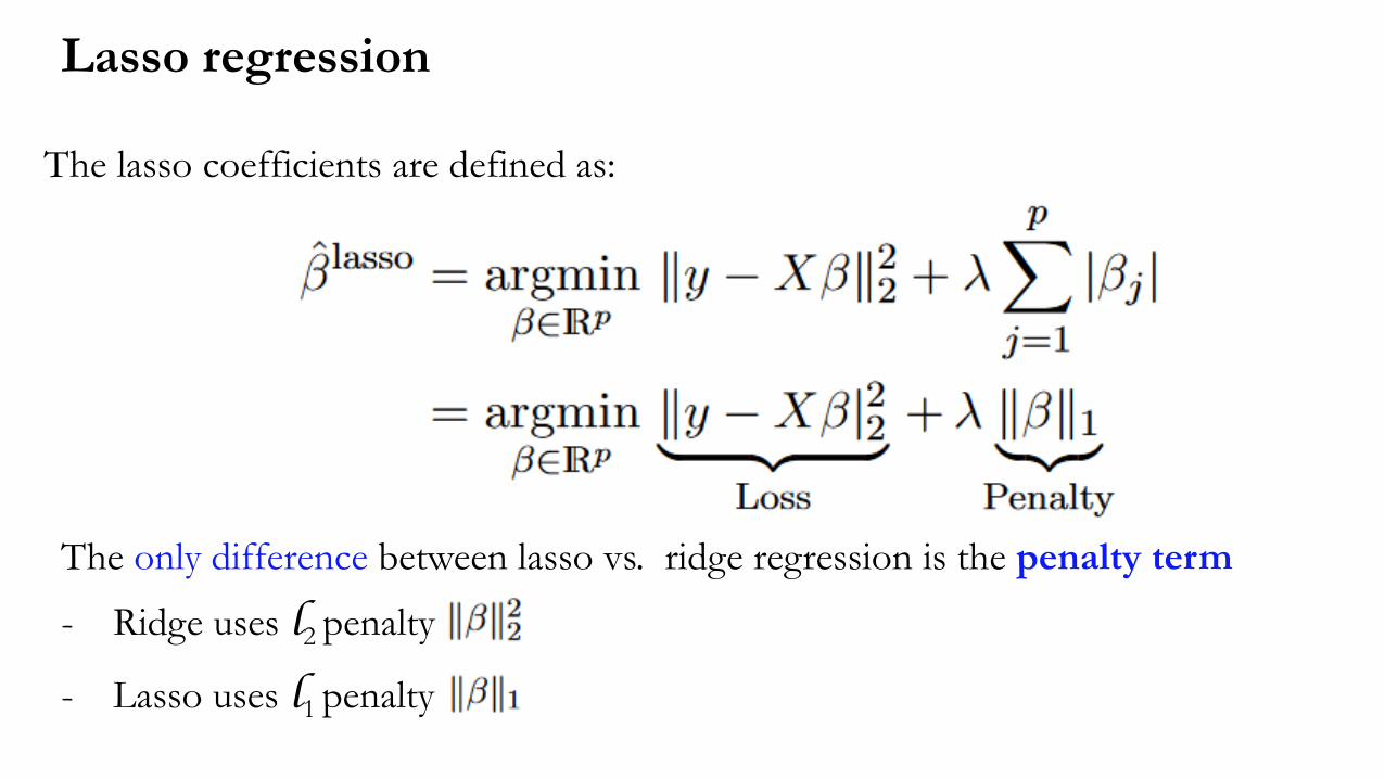
Lasso regression
The lasso coefficients are defined as:
The only difference between lasso vs. ridge regression is the penalty term
- Ridge uses l2 penalty
- Lasso uses l1 penalty
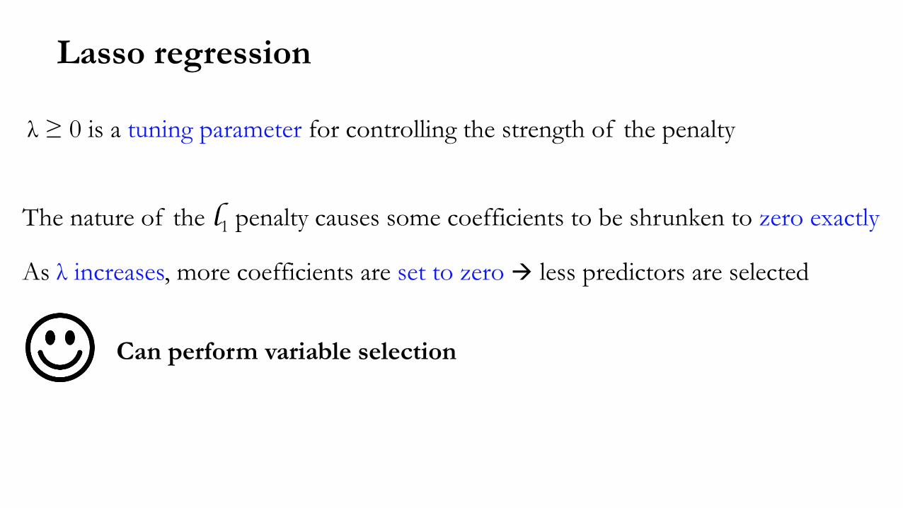
λ ≥ 0 is a tuning parameter for controlling the strength of the penalty
Lasso regression
The nature of the l1 penalty causes some coefficients to be shrunken to zero exactly
Can perform variable selection
As λ increases, more coefficients are set to zero less predictors are selected
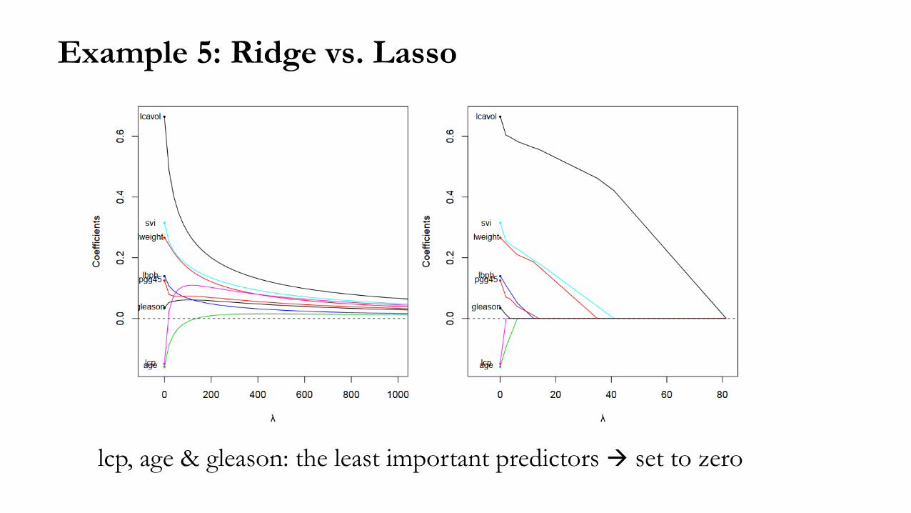
Example 5: Ridge vs. Lasso
lcp, age & gleason: the least important predictors set to zero
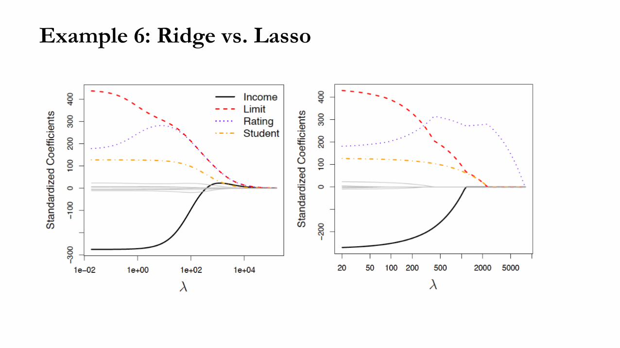
Example 6: Ridge vs. Lasso
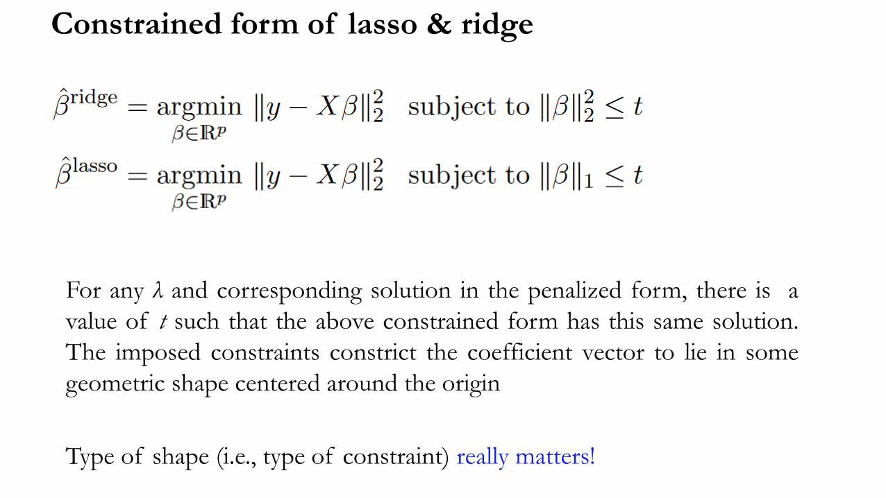
Constrained form of lasso & ridge
For any λ and corresponding solution in the penalized form, there is a
value of t such that the above constrained form has this same solution.
The imposed constraints constrict the coefficient vector to lie in some
geometric shape centered around the origin
Type of shape (i.e., type of constraint) really matters!
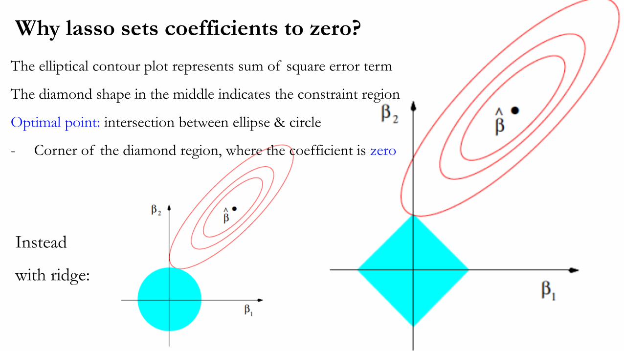
The elliptical contour plot represents sum of square error term
The diamond shape in the middle indicates the constraint region
Optimal point: intersection between ellipse & circle
- Corner of the diamond region, where the coefficient is zero
Instead
with ridge:
Why lasso sets coefficients to zero?
Regularization penalizes hypothesis complexity
• L2 regularization leads to small weights
• L1 regularization leads to many zero weights (sparsity)
• Feature selection tries to discard irrelevant features
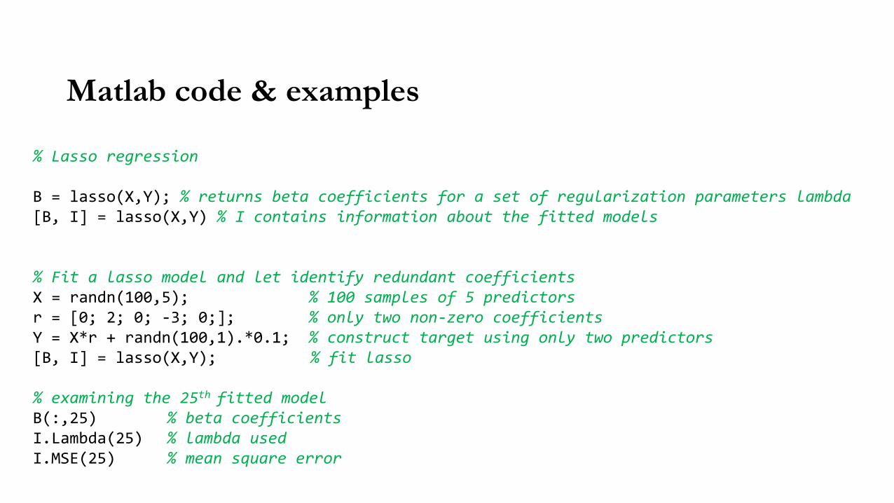
Matlab code & examples
% Lasso regression
B = lasso(X,Y); % returns beta coefficients for a set of regularization parameters lambda[B, I] = lasso(X,Y) % I contains information about the fitted models
% Fit a lasso model and let identify redundant coefficientsX = randn(100,5); % 100 samples of 5 predictorsr = [0; 2; 0; -3; 0;]; % only two non-zero coefficientsY = X*r + randn(100,1).*0.1; % construct target using only two predictors[B, I] = lasso(X,Y); % fit lasso
% examining the 25th fitted modelB(:,25) % beta coefficientsI.Lambda(25) % lambda usedI.MSE(25) % mean square error
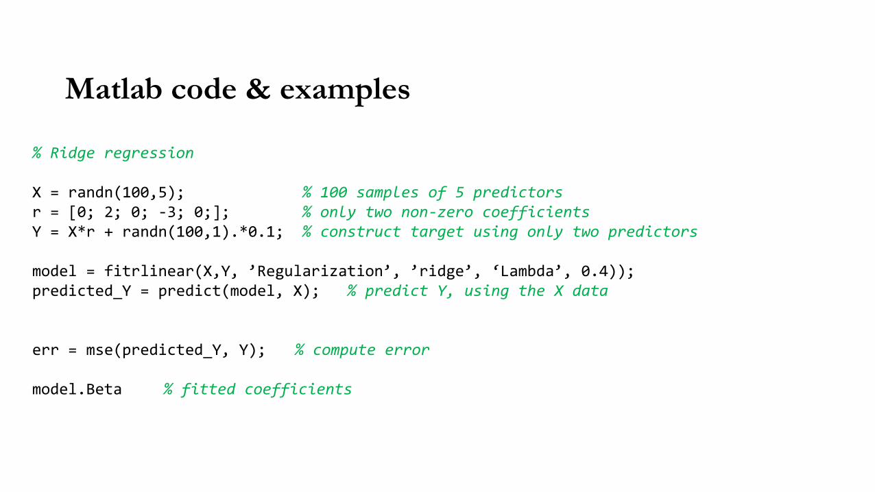
Matlab code & examples
% Ridge regression
X = randn(100,5); % 100 samples of 5 predictorsr = [0; 2; 0; -3; 0;]; % only two non-zero coefficientsY = X*r + randn(100,1).*0.1; % construct target using only two predictors
model = fitrlinear(X,Y, ’Regularization’, ’ridge’, ‘Lambda’, 0.4));predicted_Y = predict(model, X); % predict Y, using the X data
err = mse(predicted_Y, Y); % compute error
model.Beta % fitted coefficients
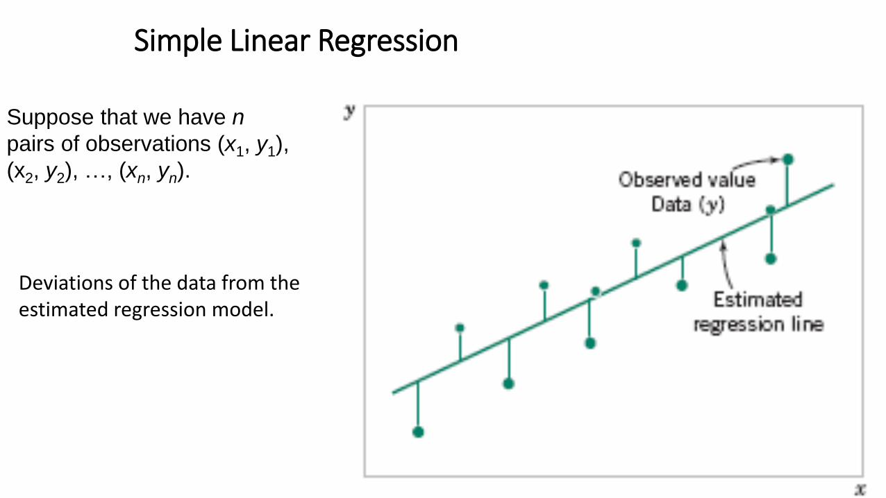
Simple Linear Regression
Suppose that we have n
pairs of observations (x1, y1),
(x2, y2), …, (xn, yn).
Deviations of the data from the estimated regression model.
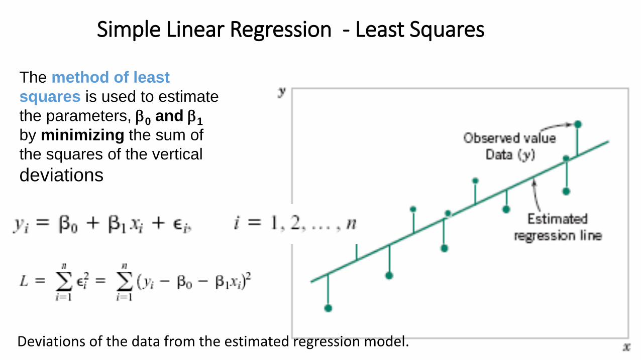
Simple Linear Regression - Least Squares
The method of least
squares is used to estimate
the parameters, 0 and 1
by minimizing the sum of
the squares of the vertical
deviations
Deviations of the data from the estimated regression model.