1

LECTURE ONE

SET THEORY

Lecture Outlines

1.1 Introduction

1.2 Objectives

1.3 Definitions of Set Concepts

1.4 Set Operations and Set Algebra

1.5 Summary

1.1 Introduction

Welcome to the First Lecture in this course unit. In this lecture we are going to learn about

set theory.

The study of sets is important and thus popular in the business and economic world for three

major reasons:

- Basic understanding of concepts in sets and set algebra provides a form of logical

language through which business specialists can communicate important concepts and

ideas.

- Set algebra is used in solving counting problems of a logical nature.

- The study of set algebra provides a solid background to understanding of probability

and statistics, which are important business decision-making tools.

1.2

Objectives

At the end of this lecture you should be able to:

1. Define a set and set concepts.

2. Use venn diagrams to illustrate sets

3. Perform set operations

1.3 Definitions and Basic Concepts

1. Definition of a set:

A set is a well-defined collection or group of objects. For instance,

- Set of all courses offered at the School of Business, University of Nairobi.

2

- Set of all European manufactured Mobile Phones in Kenya.

- Set of all female students pursuing a medical degree in Kenyan Universities.

These objects are also referred to as members or elements of a set.

Requirements of a set

(i) A set must be well defined i.e. it must not leave any room for ambiguities e.g. Set of

all students. This raises such questions as which students? Where are these students?

What is the time frame, i.e. when?

A well defined set could be a: Set of all female students pursuing a medical degree in

Kenyan Universities in the year 2010.

(ii) The elements of a given set must be distinct i.e. each object will appear once and once

only. This means that an element must appear but only once.

The following therefore does not qualify to be a set since the element 2 is repeated:

{1, 2, 4, 2, 7}.

The correct set is {1, 2, 4, 7}

(iii) The order of presenting the elements of a set is immaterial.

Thus the following four sets are the same: {1, 3, 2} = {1, 2, 3} = {3, 2, 1} = {2, 1, 3}

2. Specifying or naming of sets

By convention, sets are specified (named) using a capital letter. Further, the elements of a set

are designated by either listing all the elements or by using a descriptive characteristic or

pattern. The elements of a set are enclosed using curly brackets. For example, consider the

set of whole numbers from 0 to 6, inclusive. We can represent them in 3 ways as follows:

- Listing of all elements

A = {0, 1, 2, 3, 4, 5, 6}

- Using a descriptive characteristic

A = {X such that X is a positive integer from 0 to 6, inclusive}

- Using a pattern

3

A = {0, 1, 2 - - - - - 6}

3. Set membership

Set membership is expressed by using the Greek letter epsilon; є.

Consider set A above (used to illustrate naming of sets) in which 3 is a member. This is

expressed as: 3 є A

This can also be used in a plural sense as follows: 0, 5, 1 є A (zero, five and one are

members of set A)

4. Finite set

This is a set that consists of a limited or countable number of elements e.g. set A above

because it has 7 elements.

An infinite set therefore consists of an unlimited or uncountable number of members, e.g. set

of all odd numbers.

5. Subset

Any set say S is a subset of set A above if all elements in S are members of A. It is denoted

using the symbol;

E.g. S A which is read as “Set S is a subset of set A”

If S = {1, 5} then S A.

Recall A = {0, 1, 2, 3, 4, 5, 6}

Equally, set A is said to be the superset to set S and is denoted using the symbol;

Hence, A S

6. Equality of sets

If all elements in set D1 are also in D2 and all elements in D2 are also in D1, then;

sets D1 and D2 are equal, that is, D1 = D2

e.g. If D1 = { a, c, f } and D2 = {c, f, a }

then D1 = D2

4

Further, D1 D2 and D2 D1, that is, each set is a subset and superset to itself.

7. Universal set.

It is that set which contains all elements under consideration by the analyst or researcher and

id denoted by the symbol; U

For example if U = {all University of Nairobi students), we can have the following subsets:

S1 = {students at Lower Kabete campus}

S2 = {Male students}

S3 = {Students studying Engineering}

8. Null or empty set

This is a set with no elements. It is denoted by the notation; { } or

where is the Greek letter phi.

A good example would be a set of living human beings who are over 200 years old. Since

we cannot find such a person, this is said to be an empty set.

9. Complement of a set

If U Universal set and A is a subset of the universal set, then, the complement of A,

denoted AI or A

C represents all elements in the universal set which are not members of set A.

E.g If A = {whole numbers from 0 to 6}

and U= {whole numbers from 0 to 10} then AI = {7, 8, 9, 10}

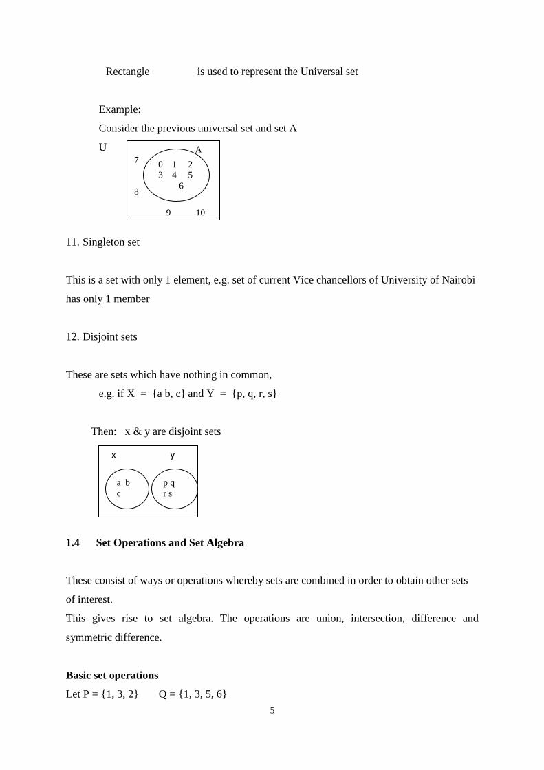
10. Sets are pictorially represented using Venn diagrams (so named after the 18th

Century

English logician, John Venn)

Symbols

Circle: (is used to represent an Ordinary set ((not a universal set)

5

Rectangle is used to represent the Universal set

Example:

Consider the previous universal set and set A

U

11. Singleton set

This is a set with only 1 element, e.g. set of current Vice chancellors of University of Nairobi

has only 1 member

12. Disjoint sets

These are sets which have nothing in common,

e.g. if X = {a b, c} and Y = {p, q, r, s}

Then: x & y are disjoint sets

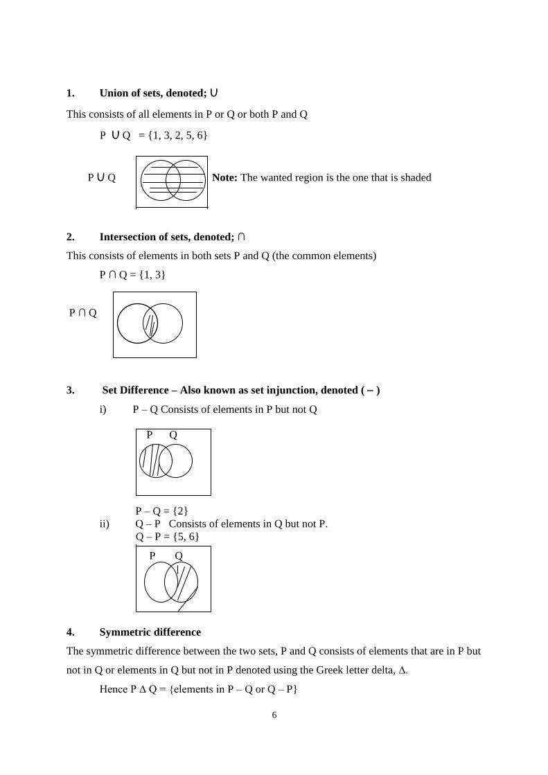
1.4 Set Operations and Set Algebra

These consist of ways or operations whereby sets are combined in order to obtain other sets

of interest.

This gives rise to set algebra. The operations are union, intersection, difference and

symmetric difference.

Basic set operations

Let P = {1, 3, 2} Q = {1, 3, 5, 6}

x y

a b

c

p q

r s

A

7

8

9 10

0 1 2

3 4 5

6

6

1. Union of sets, denoted; U

This consists of all elements in P or Q or both P and Q

P U Q = {1, 3, 2, 5, 6}

P U Q Note: The wanted region is the one that is shaded

2. Intersection of sets, denoted; ∩

This consists of elements in both sets P and Q (the common elements)

P ∩ Q = {1, 3}

P ∩ Q

3. Set Difference – Also known as set injunction, denoted ( )

i) P – Q Consists of elements in P but not Q

P Q

P – Q = {2}

ii) Q – P Consists of elements in Q but not P.

Q – P = {5, 6}

P Q

4. Symmetric difference

The symmetric difference between the two sets, P and Q consists of elements that are in P but

not in Q or elements in Q but not in P denoted using the Greek letter delta, ∆.

Hence P ∆ Q = {elements in P – Q or Q – P}

7

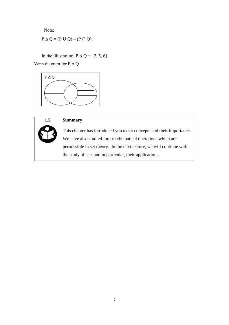
Note:

P ∆ Q = (P U Q) – (P ∩ Q)

In the illustration, P ∆ Q = {2, 5, 6}

Venn diagram for P ∆ Q

1.5

Summary

This chapter has introduced you to set concepts and their importance.

We have also studied four mathematical operations which are

permissible in set theory. In the next lecture, we will continue with

the study of sets and in particular, their applications.

P ∆ Q

8

LECTURE TWO

APPLICATION OF SET THEORY

Lecture Outlines

2.1 Introduction

2.2 Objectives

2.3 Laws of Set Algebra

2.4 Counting Problems of A Logical Nature

2.5 Summary

2.1 Introduction

Welcome to our Second Lecture. This is a continuation of the first lecture on sets. In

particular, we will learn about the consequences of set operations and their business uses.

Objectives

At the end of this lecture, you should be able to:

1. Explain the laws of set algebra.

2. Solve logical counting problems.

Laws of Set Algebra

Arising from the set operations we learned in lecture one, we have the following laws of sets:

1. Commutative laws

For any two sets P and Q,

i) P Q = Q P The order in which sets are combined with union or

intersection is irrelevant

ii) P Q = Q P

2. Associative laws

For any three sets P, Q and R,

i) (P Q) R = P (Q R) The selection of 3 or more sets for grouping in a

union or intersection is immaterial.

ii) P (Q R) = (P Q) R

2.2

9

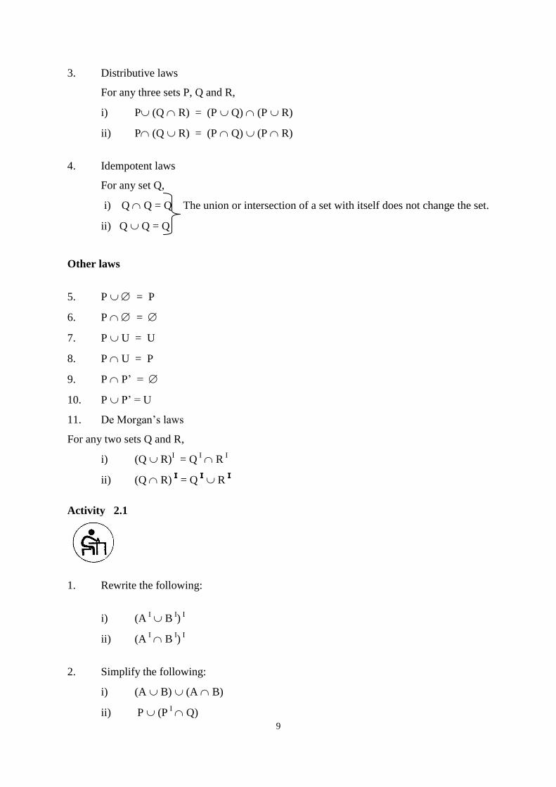
3. Distributive laws

For any three sets P, Q and R,

i) P (Q R) = (P Q) (P R)

ii) P (Q R) = (P Q) (P R)

4. Idempotent laws

For any set Q,

i) Q Q = Q The union or intersection of a set with itself does not change the set.

ii) Q Q = Q

Other laws

5. P = P

6. P =

7. P U = U

8. P U = P

9. P P’ =

10. P P’ = U

11. De Morgan’s laws

For any two sets Q and R,

i) (Q R)I = Q

I R

I

ii) (Q R) I

= Q I

R I

Activity 2.1

1. Rewrite the following:

i) (A I B

I) I

ii) (A I B

I) I

2. Simplify the following:

i) (A B) (A B)

ii) P (P I Q)

10

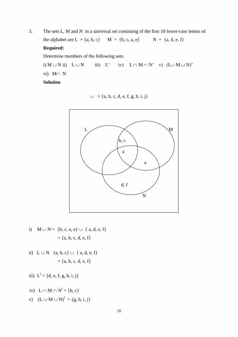
3. The sets L, M and N in a universal set consisting of the first 10 lower-case letters of

the alphabet are L = {a, b, c} M = {b, c, a, e} N = {a, d, e, f}

Required:

Determine members of the following sets:

i) M N ii) L N iii) L’ iv) L M N’ v) (L M N)’

vi) M N

Solution

= {a, b, c, d, e, f, g, h, i, j}

L M

b, c

a

e

d, f

N

i) M N = {b, c, a, e} { a, d, e, f}

= {a, b, c, d, e, f}

ii) L N {a, b, c} { a, d, e, f}

= {a, b, c, d, e, f}

iii) LI = {d, e, f, g, h, i, j}

iv) L M NI = {b, c}

v) (L M N)I = {g, h, i, j}

11

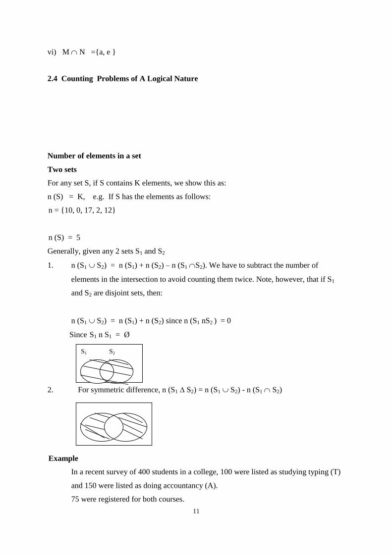
vi) M N ={a, e }

2.4 Counting Problems of A Logical Nature

Number of elements in a set

Two sets

For any set S, if S contains K elements, we show this as:

n (S) = K, e.g. If S has the elements as follows:

n = {10, 0, 17, 2, 12}

n (S) = 5

Generally, given any 2 sets S1 and S2

1. n (S1 S2) = n (S1) + n (S2) – n (S1 S2). We have to subtract the number of

elements in the intersection to avoid counting them twice. Note, however, that if S1

and S2 are disjoint sets, then:

n (S1 S2) = n (S1) + n (S2) since n (S1 nS2 ) = 0

Since S1 n S1 = Ø

2. For symmetric difference, n (S1 ∆ S2) = n (S1 S2) - n (S1 S2)

Example

In a recent survey of 400 students in a college, 100 were listed as studying typing (T)

and 150 were listed as doing accountancy (A).

75 were registered for both courses.

S1 S2

12

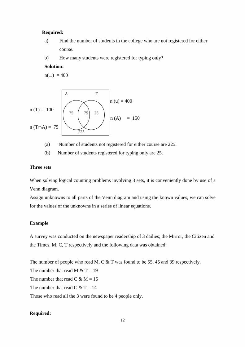
Required:

a) Find the number of students in the college who are not registered for either

course.

b) How many students were registered for typing only?

Solution:

n() = 400

n (u) = 400

n (T) = 100

n (A) = 150

n (TA) = 75

(a) Number of students not registered for either course are 225.

(b) Number of students registered for typing only are 25.

Three sets

When solving logical counting problems involving 3 sets, it is conveniently done by use of a

Venn diagram.

Assign unknowns to all parts of the Venn diagram and using the known values, we can solve

for the values of the unknowns in a series of linear equations.

Example

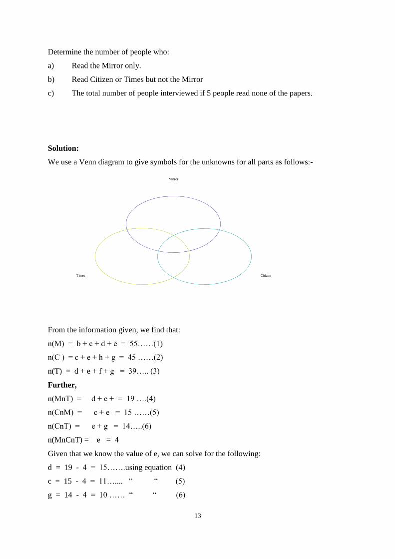
A survey was conducted on the newspaper readership of 3 dailies; the Mirror, the Citizen and

the Times, M, C, T respectively and the following data was obtained:

The number of people who read M, C & T was found to be 55, 45 and 39 respectively.

The number that read M & T = 19

The number that read C & M = 15

The number that read C & T = 14

Those who read all the 3 were found to be 4 people only.

Required:

A T

225

75

75 25

13

Determine the number of people who:

a) Read the Mirror only.

b) Read Citizen or Times but not the Mirror

c) The total number of people interviewed if 5 people read none of the papers.

Solution:

We use a Venn diagram to give symbols for the unknowns for all parts as follows:-

From the information given, we find that:

n(M) = b + c + d + e = 55……(1)

n(C ) = c + e + h + g = 45 ……(2)

n(T) = d + e + f + g = 39….. (3)

Further,

n(MnT) = d + e + = 19 ….(4)

n(CnM) = c + e = 15 ……(5)

n(CnT) = e + g = 14…..(6)

n(MnCnT) = e = 4

Given that we know the value of e, we can solve for the following:

d = 19 - 4 = 15…….using equation (4)

c = 15 - 4 = 11….... “ “ (5)

g = 14 - 4 = 10 …… “ “ (6)

Mirror

Citizen Times

14

Using equation (1), we find that :

b = 55 - (11 + 15 + 4)

= 15

Using equation (2):

h = 45 - (11 + 4 + 10) = 20

Using equation (3):

f = 39 - (15 + 4 + 10)

= 10

If 5 people read none of the three dailies, then a = 5

Let us now answer specific questions asked:

a) n(M only) = b = 5

b) n(C or T but not M) = 20 + 10 + 10

= 4

c) n(U) = 5 + 25 + 11 + 15 + 4 + 10 + 10 + 20

= 100

2.5

Summary

This lecture has dealt with the postulates or laws of set theory. This

arises from the permissible set operations. Also studied has been the

application of set algebra to logical counting problems.

Activity 2.2

Self Test One

a) A company has a large of computer assistants, each of whom

is competent in the use of at least one of 3 utility packages:

Word processor (W) Database Management system (D) and a

Spreadsheet (S). A survey shows that 30 can use a word

processor, 25 can use a Database Management system and 28

are competent in the use of a Spreadsheet. Of the computer

15

facility assistants who can use a Database Management

System, 14 can also use a word processor while 6 have no

other skill.

6 of the computer assistants can use a word processor and

spreadsheet but not a database system while 4 have all three

skills.

Required:

Determine the number of computer facility assistants who are

members of the following sets:

i) W D S’

ii) (W S)’ S

iii) D S

iv) Universal set

b) A sample of 100 Young Christian Union voters revealed the

following concerning three candidates;

Ali, Bungei and Chiru, who were running for the Y.C.S Party

Chairman, Secretary and Treasurer respectively.

14 preferred booth Ali and Bungei

49 preferred Ali or Bungei but not Chiru

21 preferred Bungei but not Chiru or Ali

61 preferred Bungei or Chiru but not Ali

32 preferred Chiru but not Ali or Bungei

7 preferred Ali and Chiru but not Bungei.

Required:

i) With the aid of a Venn diagram, determine the number of

voters that were in favor of all the three candidates. Assume

that every member of Y.C.S voted for at least one candidate.

Determine the candidate that went unopposed if a rule of 50%

majority were used in such a decision.

16

LECTURE THREE

FUNCTIONS

Lecture outlines

3.1 Introduction

3.2 Objectives

3.3. Preliminary Concepts and Definitions

3.3.1 Preliminary Concepts

3.3.2 Definitions

3.3.3 Importance of Functions in Business

3.4 Types of Functions

3.5 Linear functions and Applications

3.4.1 Constant Functions

3.4.2 Polynomial Functions

3.4.3 Multivariate Functions

3.4.4 Logarithmic Functions

3.4.5 Exponential Functions

3.4.6 Continuous Vs Discrete Functions

3.4.7 Step Functions

3.5.1What is Linear Function

3.5.2 Application of Linear Functions in Business World

3.1 Introduction

Welcome to the Third Lecture of this unit. In this unit, we shall learn about relationships

which are known as functions.

17

Objectives

At the end of this lecture, you should be able to:

1. Define a function.

2. Describe various types of functions.

3. Describe a linear function and its characteristics.

4. Sketch the graph of a linear function.

5. Fit a linear function given a set of data.

6. Apply linear functions in solving business problems.

3.3. Preliminary Concepts and Definitions

3.3.1 Preliminary Concepts

Before we define a function, there are certain preliminary ideas which we require to

understand.

1. A CONSTANT: Is a quantity whose value remains unchanged throughout a

particular analysis

e.g. a fixed cost such as salary or rent in a given period.

2. A VARIABLE: Is a quantity, which assumes or takes various values in a

particular analysis.

Examples

Suppose an item is sold for Shs.35 per unit and

Let S = Sales revenue

Q = Quantity sold

The price of Sh.35 is a constant but sales revenue (S) and quantity sold (Q) are variables.

However, these variables are of two types: independent variable and dependent variable.

Independent and Dependent Variable

An independent capable is the one that determines the quantity or the value of some other

variable, which is then termed the dependent variable.

For the preceding illustration, quantity sold (Q) is the independent variable whereas sales

revenue (S) is the dependent variable.

Furthermore, since quantity sold “predicts” the sales revenue, which in turn “response” to

sales quantity, Q is also called predictor variable and S the response variable.

3.2

18

3.3.2 Definition

A function is a relationship in which values of a dependent variable are determined by the

values of one or more independent variable or variables. We use the letter f to express a

function. An example is: “Sales is a function of quantity” is expressed as: Sales = f

(quantity).

Types of mappings (Relationships)

Similarly, Savings = f (Income)

Demand = f (Price, income, price of related goods, etc)

Take Note

- Dependent variables is only one

- Independent variables can be one or more

3.3.3 Importance of Functions in Business

Functions are important in establishing relationships among business variables which

facilitates their control for achieving organizational objectives, e.g. in making decisions such

as:

- Output required

- Prices to charge

- Level of advertising

- Optimal workforce size, etc.

3.4 Types of Functions

Some of the more commonly encountered functions in the business world include the

following:

19

a) Constant functions

b) Polynomial functions

c) Multivariate functions

d) Logarithmic functions

e) Exponential, functions

f) Continuous Versus discrete functions

g) Step function

We will now have a brief explanation of each of these types of functions.

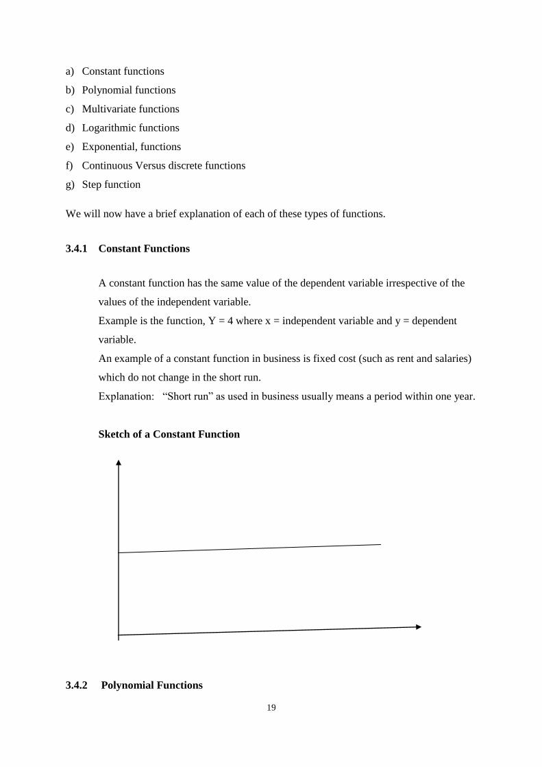
3.4.1 Constant Functions

A constant function has the same value of the dependent variable irrespective of the

values of the independent variable.

Example is the function, Y = 4 where x = independent variable and y = dependent

variable.

An example of a constant function in business is fixed cost (such as rent and salaries)

which do not change in the short run.

Explanation: “Short run” as used in business usually means a period within one year.

Sketch of a Constant Function

3.4.2 Polynomial Functions

20

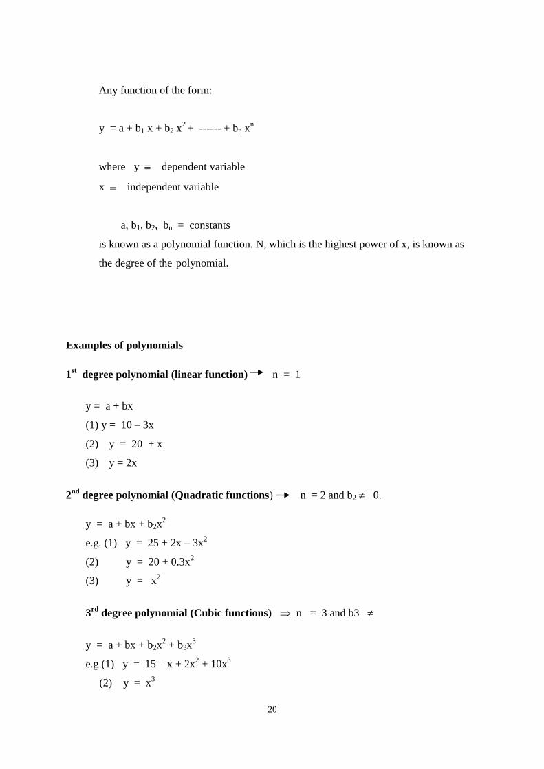
Any function of the form:

y = a + b1 x + b2 x2 + ------ + bn x

n

where y dependent variable

x independent variable

a, b1, b2, bn = constants

is known as a polynomial function. N, which is the highest power of x, is known as

the degree of the polynomial.

Examples of polynomials

1st degree polynomial (linear function) n = 1

y = a + bx

(1) y = 10 – 3x

(2) y = 20 + x

(3) y = 2x

2nd

degree polynomial (Quadratic functions) n = 2 and b2 0.

y = a + bx + b2x2

e.g. (1) y = 25 + 2x – 3x2

(2) y = 20 + 0.3x2

(3) y = x2

3rd

degree polynomial (Cubic functions) n = 3 and b3

y = a + bx + b2x2 + b3x

3

e.g (1) y = 15 – x + 2x2 + 10x

3

(2) y = x3

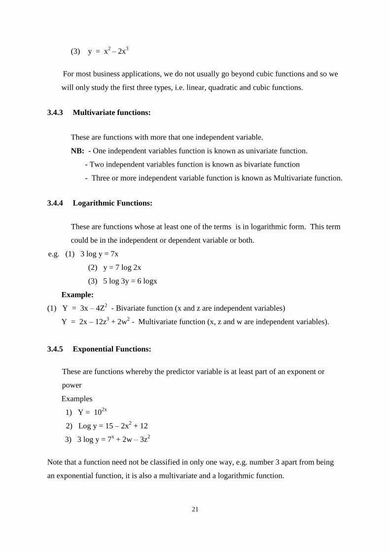
21

(3) y = x2

– 2x3

For most business applications, we do not usually go beyond cubic functions and so we

will only study the first three types, i.e. linear, quadratic and cubic functions.

3.4.3 Multivariate functions:

These are functions with more that one independent variable.

NB: - One independent variables function is known as univariate function.

- Two independent variables function is known as bivariate function

- Three or more independent variable function is known as Multivariate function.

3.4.4 Logarithmic Functions:

These are functions whose at least one of the terms is in logarithmic form. This term

could be in the independent or dependent variable or both.

e.g. (1) 3 log y = 7x

(2) y = 7 log 2x

(3) 5 log 3y = 6 logx

Example:

(1) Y = 3x – 4Z2 - Bivariate function (x and z are independent variables)

Y = 2x – 12z3 + 2w

2 - Multivariate function (x, z and w are independent variables).

3.4.5 Exponential Functions:

These are functions whereby the predictor variable is at least part of an exponent or

power

Examples

1) Y = 102x

2) Log y = 15 – 2x2 + 12

3) 3 log y = 7x + 2w – 3z

2

Note that a function need not be classified in only one way, e.g. number 3 apart from being

an exponential function, it is also a multivariate and a logarithmic function.

22

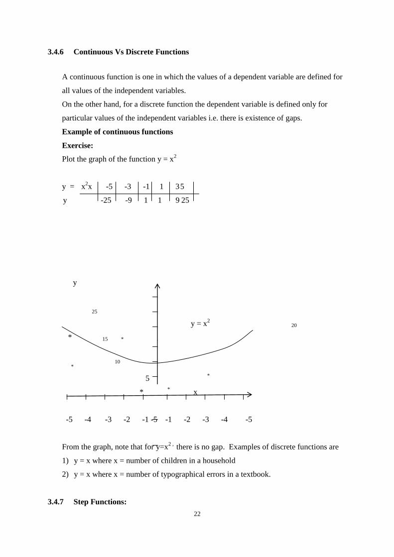
3.4.6 Continuous Vs Discrete Functions

A continuous function is one in which the values of a dependent variable are defined for

all values of the independent variables.

On the other hand, for a discrete function the dependent variable is defined only for

particular values of the independent variables i.e. there is existence of gaps.

Example of continuous functions

Exercise:

Plot the graph of the function y = x2

y = x2 x -5 -3 -1 1 3 5

y -25 -9 1 1 9 25

y

25

y = x2

20

* 15 *

* 10

5 *

* *

x

-5 -4 -3 -2 -1 -5 -1 -2 -3 -4 -5

From the graph, note that for y=x2 ,

there is no gap. Examples of discrete functions are

1) y = x where x = number of children in a household

2) y = x where x = number of typographical errors in a textbook.

3.4.7 Step Functions:

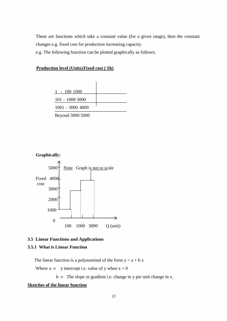
23

These are functions which take a constant value (for a given range), then the constant

changes e.g. fixed cost for production increasing capacity.

e.g. The following function can be plotted graphically as follows:

Production level (Units) Fixed cost ( Sh)

1 - 100 1000

101 – 1000 3000

1001 – 3000 4000

Beyond 3000 5000

Graphically:

5000 Note. Graph is not to scale

Fixed 4000

cost

3000

2000

1000

0

100 1000 3000 Q (unit)

3.5 Linear Functions and Applications

3.5.1 What is Linear Function

The linear function is a polynominal of the form y = a + b x

Where a y intercept i.e. value of y when x = 0

b The slope or gradient i.e. change in y per unit change in x.

Sketches of the linear function

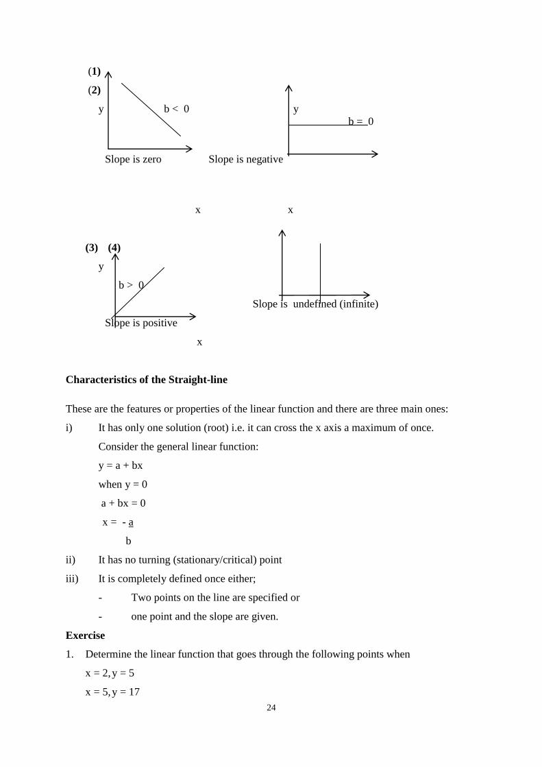
24

(1)

(2)

y b < 0 y

b = 0

Slope is zero Slope is negative

x x

(3) (4)

y

b > 0

Slope is undefined (infinite)

Slope is positive

x

Characteristics of the Straight-line

These are the features or properties of the linear function and there are three main ones:

i) It has only one solution (root) i.e. it can cross the x axis a maximum of once.

Consider the general linear function:

y = a + bx

when y = 0

a + bx = 0

x = - a

b

ii) It has no turning (stationary/critical) point

iii) It is completely defined once either;

- Two points on the line are specified or

- one point and the slope are given.

Exercise

1. Determine the linear function that goes through the following points when

x = 2, y = 5

x = 5, y = 17

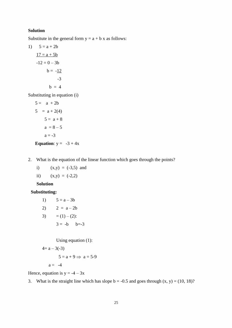
25

Solution

Substitute in the general form y = a + b x as follows:

1) 5 = a + 2b

17 = a + 5b

-12 = 0 – 3b

b = -12

-3

b = 4

Substituting in equation (i)

5 = a + 2b

5 = a + 2(4)

5 = a + 8

a = 8 – 5

a = -3

Equation: y = -3 + 4x

2. What is the equation of the linear function which goes through the points?

i) (x,y) = (-3,5) and

ii) (x,y) = (-2,2)

Solution

Substituting:

1) 5 = a – 3b

2) 2 = a – 2b

3) = (1) – (2):

3 = -b b=-3

Using equation (1):

4= a – 3(-3)

5 = a + 9 a = 5-9

a = -4

Hence, equation is y = -4 – 3x

3. What is the straight line which has slope b = -0.5 and goes through (x, y) = (10, 18)?

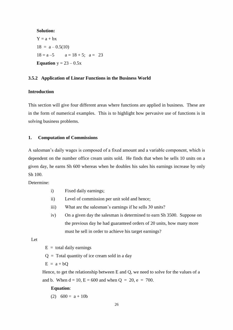
26

Solution:

Y = a + bx

18 = a – 0.5(10)

18 = a –5 a = 18 + 5; a = 23

Equation y = 23 – 0.5x

3.5.2 Application of Linear Functions in the Business World

Introduction

This section will give four different areas where functions are applied in business. These are

in the form of numerical examples. This is to highlight how pervasive use of functions is in

solving business problems.

1. Computation of Commissions

A salesman’s daily wages is composed of a fixed amount and a variable component, which is

dependent on the number office cream units sold. He finds that when he sells 10 units on a

given day, he earns Sh 600 whereas when he doubles his sales his earnings increase by only

Sh 100.

Determine:

i) Fixed daily earnings;

ii) Level of commission per unit sold and hence;

iii) What are the salesman’s earnings if he sells 30 units?

iv) On a given day the salesman is determined to earn Sh 3500. Suppose on

the previous day he had guaranteed orders of 20 units, how many more

must he sell in order to achieve his target earnings?

Let

E = total daily earnings

Q = Total quantity of ice cream sold in a day

E = a + bQ

Hence, to get the relationship between E and Q, we need to solve for the values of a

and b. When d = 10, E = 600 and when Q = 20, e = 700.

Equation:

(2) 600 = a + 10b

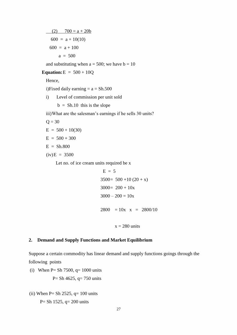
27

(2) 700 = a + 20b

600 = a + 10(10)

600 = a + 100

a = 500

and substituting when a = 500; we have b = 10

Equation: E = 500 + 10Q

Hence,

i) Fixed daily earning = a = Sh.500

i) Level of commission per unit sold

b = Sh.10 this is the slope

iii) What are the salesman’s earnings if he sells 30 units?

Q = 30

E = 500 + 10(30)

E = 500 + 300

E = Sh.800

(iv) E = 3500

Let no. of ice cream units required be x

E = 5

3500 = 500 +10 (20 + x)

3000 = 200 + 10x

3000 – 200 = 10x

2800 = 10x x = 2800/10

x = 280 units

2. Demand and Supply Functions and Market Equilibrium

Suppose a certain commodity has linear demand and supply functions goings through the

following points

(i) When P= Sh 7500, q= 1000 units

P= Sh 4625, q= 750 units

(ii) When P= Sh 2525, q= 100 units

P= Sh 1525, q= 200 units

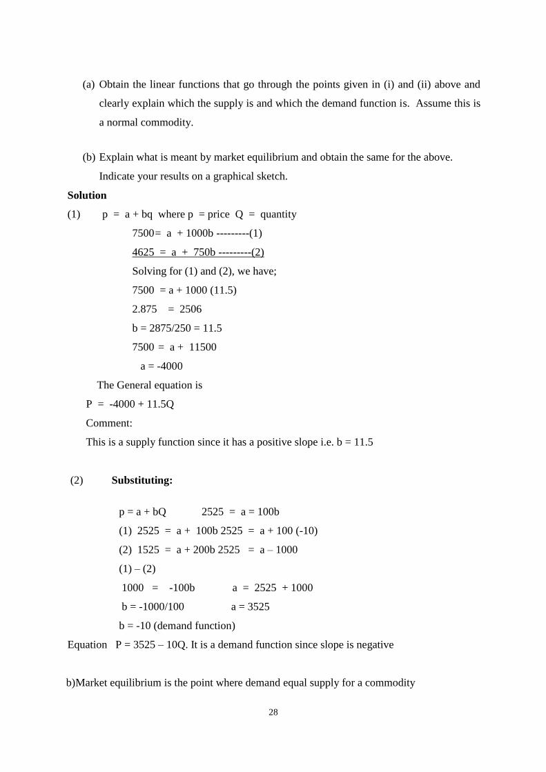
28

(a) Obtain the linear functions that go through the points given in (i) and (ii) above and

clearly explain which the supply is and which the demand function is. Assume this is

a normal commodity.

(b) Explain what is meant by market equilibrium and obtain the same for the above.

Indicate your results on a graphical sketch.

Solution

(1) p = a + bq where p = price Q = quantity

7500 = a + 1000b ---------(1)

4625 = a + 750b ---------(2)

Solving for (1) and (2), we have;

7500 = a + 1000 (11.5)

2.875 = 2506

b = 2875/250 = 11.5

7500 = a + 11500

a = -4000

The General equation is

P = -4000 + 11.5Q

Comment:

This is a supply function since it has a positive slope i.e. b = 11.5

(2) Substituting:

p = a + bQ 2525 = a = 100b

(1) 2525 = a + 100b 2525 = a + 100 (-10)

(2) 1525 = a + 200b 2525 = a – 1000

(1) – (2)

1000 = -100b a = 2525 + 1000

b = -1000/100 a = 3525

b = -10 (demand function)

Equation P = 3525 – 10Q. It is a demand function since slope is negative

b) Market equilibrium is the point where demand equal supply for a commodity

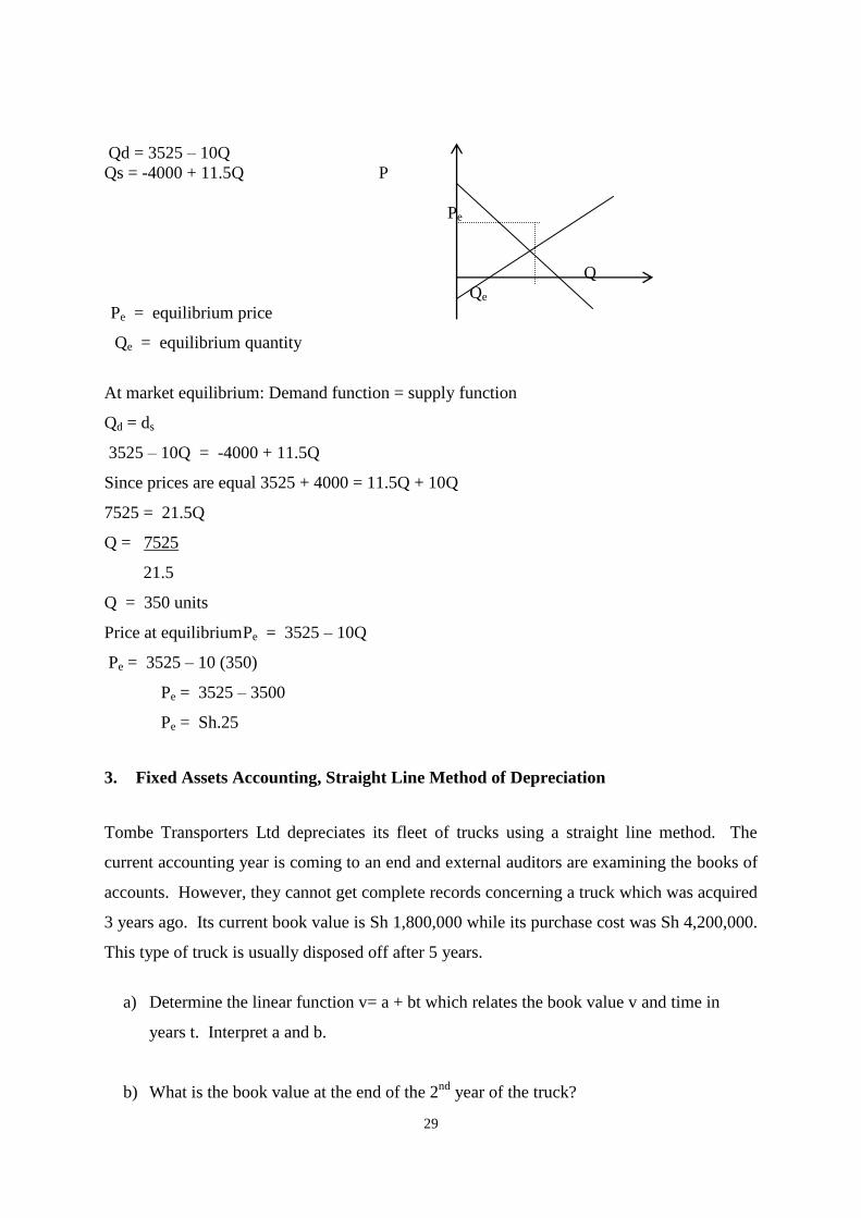
29

Qd = 3525 – 10Q

Qs = -4000 + 11.5Q P

Pe

Q

Qe

Pe = equilibrium price

Qe = equilibrium quantity

At market equilibrium: Demand function = supply function

Qd = ds

3525 – 10Q = -4000 + 11.5Q

Since prices are equal 3525 + 4000 = 11.5Q + 10Q

7525 = 21.5Q

Q = 7525

21.5

Q = 350 units

Price at equilibrium Pe = 3525 – 10Q

Pe = 3525 – 10 (350)

Pe = 3525 – 3500

Pe = Sh.25

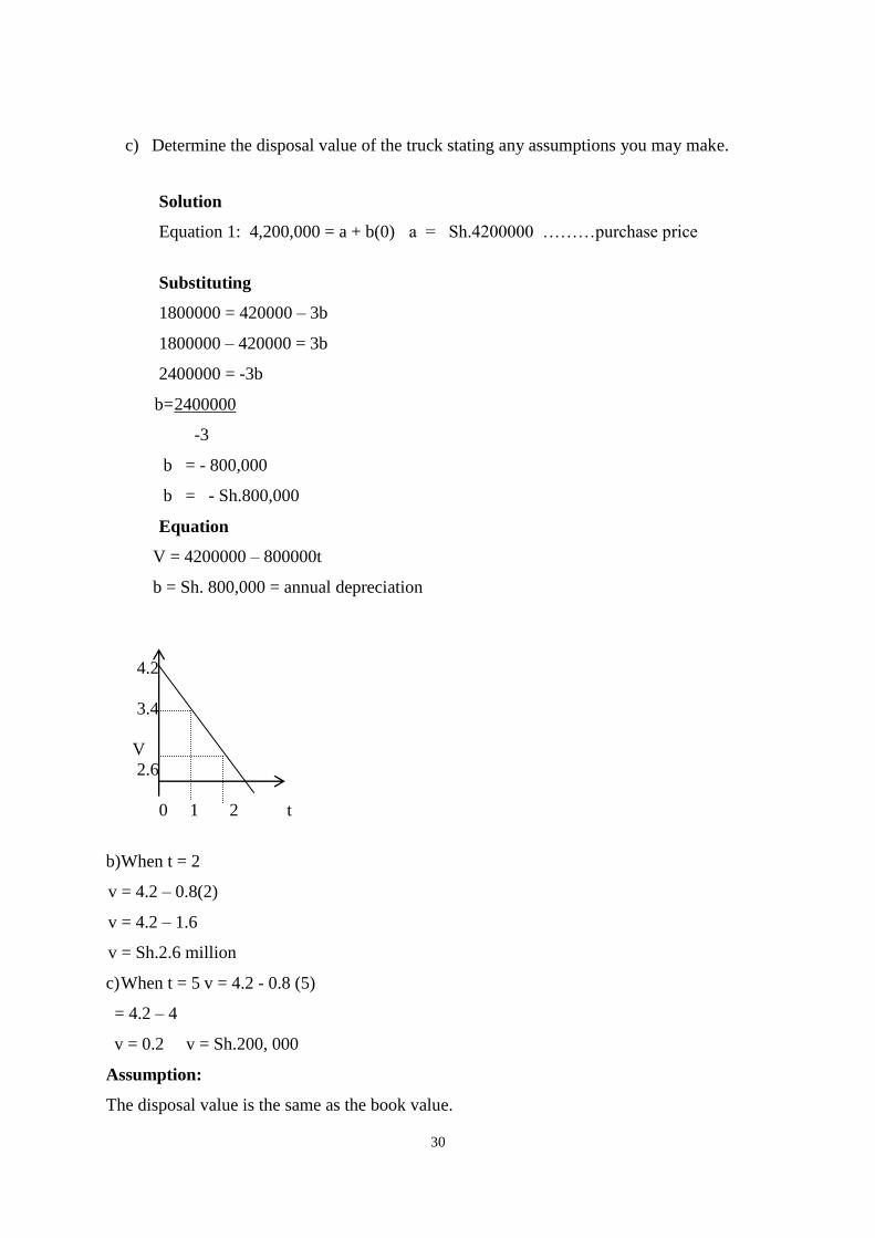
3. Fixed Assets Accounting, Straight Line Method of Depreciation

Tombe Transporters Ltd depreciates its fleet of trucks using a straight line method. The

current accounting year is coming to an end and external auditors are examining the books of

accounts. However, they cannot get complete records concerning a truck which was acquired

3 years ago. Its current book value is Sh 1,800,000 while its purchase cost was Sh 4,200,000.

This type of truck is usually disposed off after 5 years.

a) Determine the linear function v= a + bt which relates the book value v and time in

years t. Interpret a and b.

b) What is the book value at the end of the 2nd

year of the truck?

30

c) Determine the disposal value of the truck stating any assumptions you may make.

Solution

Equation 1: 4,200,000 = a + b(0) a = Sh.4200000 ………purchase price

Substituting

1800000 = 420000 – 3b

1800000 – 420000 = 3b

2400000 = -3b

b = 2400000

-3

b = - 800,000

b = - Sh.800,000

Equation

V = 4200000 – 800000t

b = Sh. 800,000 = annual depreciation

4.2

3.4

V

2.6

0 1 2 t

b) When t = 2

v = 4.2 – 0.8(2)

v = 4.2 – 1.6

v = Sh.2.6 million

c) When t = 5 v = 4.2 - 0.8 (5)

= 4.2 – 4

v = 0.2 v = Sh.200, 000

Assumption:

The disposal value is the same as the book value.

31

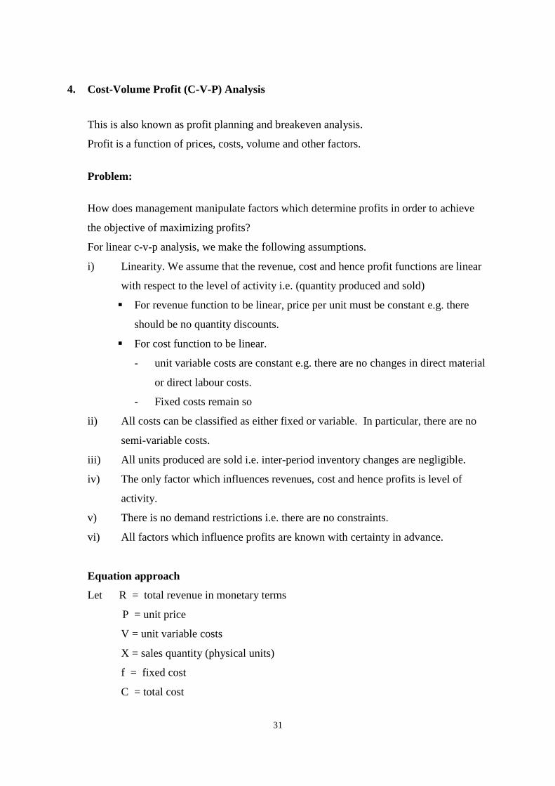
4. Cost-Volume Profit (C-V-P) Analysis

This is also known as profit planning and breakeven analysis.

Profit is a function of prices, costs, volume and other factors.

Problem:

How does management manipulate factors which determine profits in order to achieve

the objective of maximizing profits?

For linear c-v-p analysis, we make the following assumptions.

i) Linearity. We assume that the revenue, cost and hence profit functions are linear

with respect to the level of activity i.e. (quantity produced and sold)

For revenue function to be linear, price per unit must be constant e.g. there

should be no quantity discounts.

For cost function to be linear.

- unit variable costs are constant e.g. there are no changes in direct material

or direct labour costs.

- Fixed costs remain so

ii) All costs can be classified as either fixed or variable. In particular, there are no

semi-variable costs.

iii) All units produced are sold i.e. inter-period inventory changes are negligible.

iv) The only factor which influences revenues, cost and hence profits is level of

activity.

v) There is no demand restrictions i.e. there are no constraints.

vi) All factors which influence profits are known with certainty in advance.

Equation approach

Let R = total revenue in monetary terms

P = unit price

V = unit variable costs

X = sales quantity (physical units)

f = fixed cost

C = total cost

32

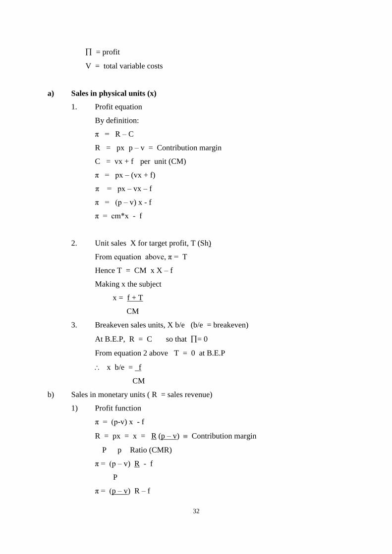
= profit

V = total variable costs

a) Sales in physical units (x)

1. Profit equation

By definition:

π = R – C

R = px p – v = Contribution margin

C = vx + f per unit (CM)

π = px – (vx + f)

π = px – vx – f

π = (p – v) x - f

π = cm*x - f

2. Unit sales X for target profit, T (Sh)

From equation above, π = T

Hence T = CM x X – f

Making x the subject

x = f + T

CM

3. Breakeven sales units, X b/e (b/e = breakeven)

At B.E.P, R = C so that = 0

From equation 2 above T = 0 at B.E.P

x b/e = f

CM

b) Sales in monetary units ( R = sales revenue)

1) Profit function

π = (p-v) x - f

R = px = x = R (p – v) Contribution margin

P p Ratio (CMR)

π = (p – v) R - f

P

π = (p – v) R – f

33

P

= CMR *( R – f)

2) Sales revenue required for target profit, T Sh

From equation above π = T

T = CMR x R – f

R = f + T

CMR

3) Sales revenue required for breakeven sales revenue, R b/e

R b/e = f

CMR

At B.E.P, = 0

Note: CMR = p

vp CMR =

p

v

p

p

p

v = Variable cost ratio (VCR)

CMR = 1 – VCR CMR + VCR = 1

Also v = Total variable costs = v x x

p Total sales p x x

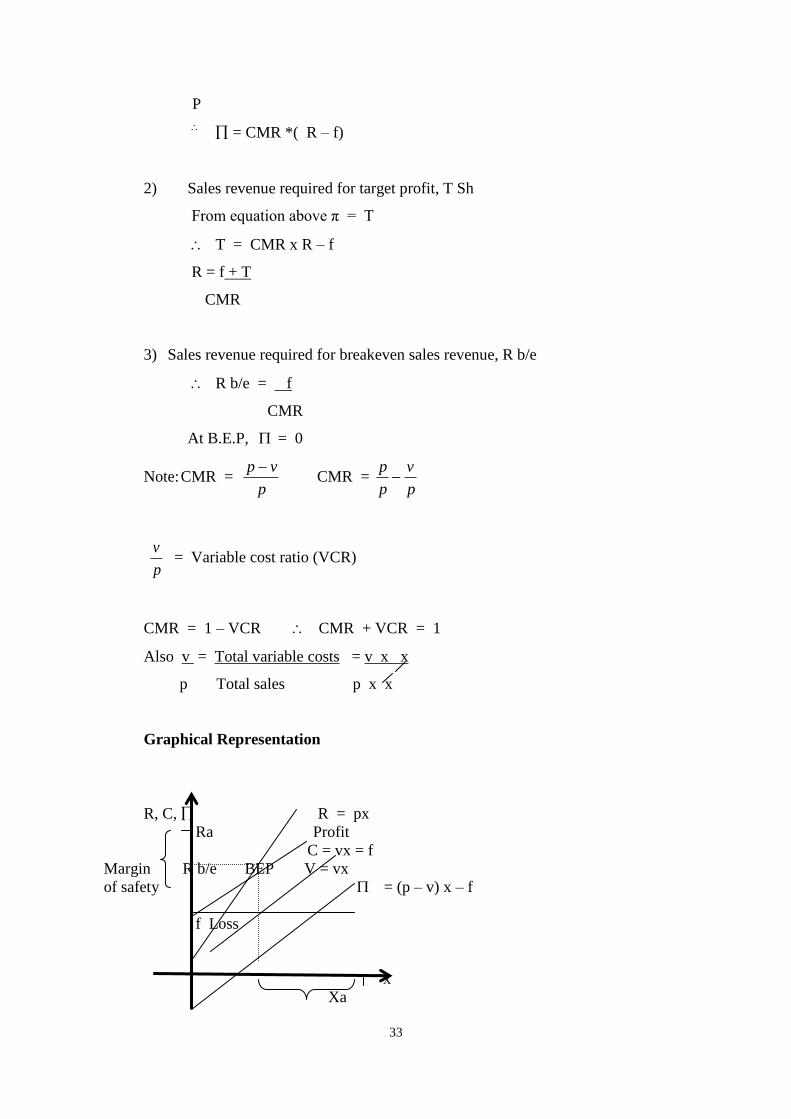
Graphical Representation

R, C, R = px

Ra Profit

C = vx = f

Margin R b/e BEP V = vx

of safety = (p – v) x – f

f Loss

x

Xa

34

-f Margin of safety

Let actual sales (beyond breakeven sales) be xa

Xa – X b/ the extent by which actual sales exceeds breakeven sales is known as

Margin of Safety (MoS).

This is also the extent by which sales would have to fall before the firm begins to

make losses.

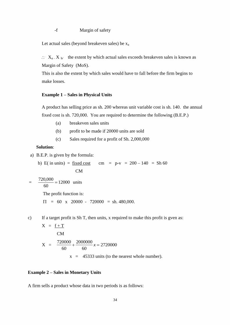
Example 1 – Sales in Physical Units

A product has selling price as sh. 200 whereas unit variable cost is sh. 140. the annual

fixed cost is sh. 720,000. You are required to determine the following (B.E.P.)

(a) breakeven sales units

(b) profit to be made if 20000 units are sold

(c) Sales required for a profit of Sh. 2,000,000

Solution:

a) B.E.P. is given by the formula:

b) E( in units) = fixed cost cm = p-v = 200 – 140 = Sh 60

CM

= 1200060

000,720 units

The profit function is:

= 60 x 20000 - 720000 = sh. 480,000.

c) If a target profit is Sh T, then units, x required to make this profit is gven as:

X = f + T

CM

X = 272000060

2000000

60

720000 x

x = 45333 units (to the nearest whole number).

Example 2 – Sales in Monetary Units

A firm sells a product whose data in two periods is as follows:

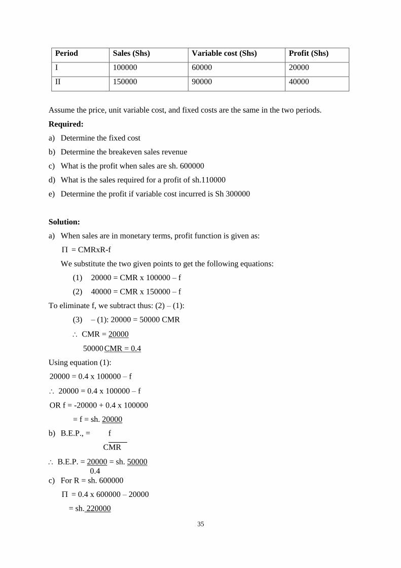
35

Period Sales (Shs) Variable cost (Shs) Profit (Shs)

I 100000 60000 20000

II 150000 90000 40000

Assume the price, unit variable cost, and fixed costs are the same in the two periods.

Required:

a) Determine the fixed cost

b) Determine the breakeven sales revenue

c) What is the profit when sales are sh. 600000

d) What is the sales required for a profit of sh.110000

e) Determine the profit if variable cost incurred is Sh 300000

Solution:

a) When sales are in monetary terms, profit function is given as:

= CMRxR-f

We substitute the two given points to get the following equations:

(1) 20000 = CMR x 100000 – f

(2) 40000 = CMR x 150000 – f

To eliminate f, we subtract thus: (2) – (1):

(3) – (1): 20000 = 50000 CMR

CMR = 20000

50000 CMR = 0.4

Using equation (1):

20000 = 0.4 x 100000 – f

20000 = 0.4 x 100000 – f

OR f = -20000 + 0.4 x 100000

= f = sh. 20000

b) B.E.P., = f

CMR

B.E.P. = 20000 = sh. 50000

0.4

c) For R = sh. 600000

= 0.4 x 600000 – 20000

= sh. 220000

36

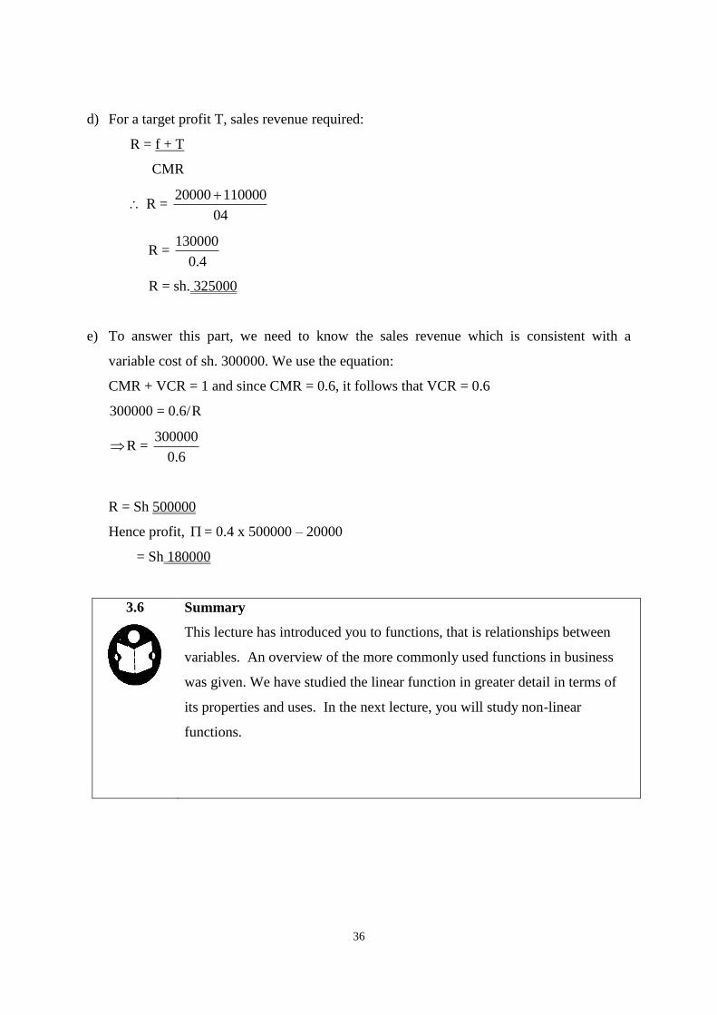
d) For a target profit T, sales revenue required:

R = f + T

CMR

R = 04

11000020000

R = 4.0

130000

R = sh. 325000

e) To answer this part, we need to know the sales revenue which is consistent with a

variable cost of sh. 300000. We use the equation:

CMR + VCR = 1 and since CMR = 0.6, it follows that VCR = 0.6

300000 = 0.6/ R

R = 6.0

300000

R = Sh 500000

Hence profit, = 0.4 x 500000 – 20000

= Sh 180000

3.6

Summary

This lecture has introduced you to functions, that is relationships between

variables. An overview of the more commonly used functions in business

was given. We have studied the linear function in greater detail in terms of

its properties and uses. In the next lecture, you will study non-linear

functions.

37

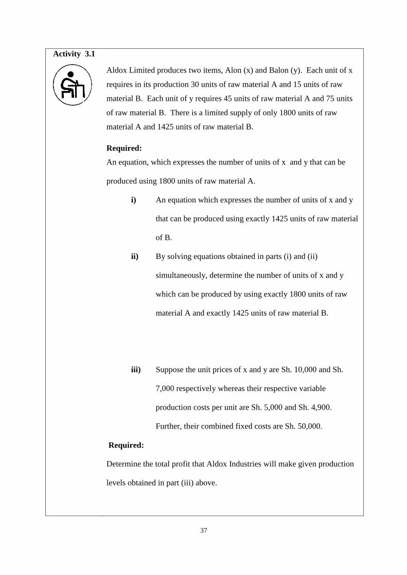
Activity 3.1

Aldox Limited produces two items, Alon (x) and Balon (y). Each unit of x

requires in its production 30 units of raw material A and 15 units of raw

material B. Each unit of y requires 45 units of raw material A and 75 units

of raw material B. There is a limited supply of only 1800 units of raw

material A and 1425 units of raw material B.

Required:

An equation, which expresses the number of units of x and y that can be

produced using 1800 units of raw material A.

i) An equation which expresses the number of units of x and y

that can be produced using exactly 1425 units of raw material

of B.

ii) By solving equations obtained in parts (i) and (ii)

simultaneously, determine the number of units of x and y

which can be produced by using exactly 1800 units of raw

material A and exactly 1425 units of raw material B.

iii) Suppose the unit prices of x and y are Sh. 10,000 and Sh.

7,000 respectively whereas their respective variable

production costs per unit are Sh. 5,000 and Sh. 4,900.

Further, their combined fixed costs are Sh. 50,000.

Required:

Determine the total profit that Aldox Industries will make given production

levels obtained in part (iii) above.

38

LECTURE FOUR

QUADRATIC AND CUBIC FUNCTIONS

Lecture Outlines

4.1 Introduction

4.2 Objectives

4.3 Quadratic Functions and Applications

4.4 Cubic Functions and Applications

4.5 Summary

4.1 Introduction

Welcome to our fourth lecture. In lecture three, we learned the properties and applications of

linear functions. This lecture is in a sense a continuation of the same concepts to quadratic

and cubic functions.

39

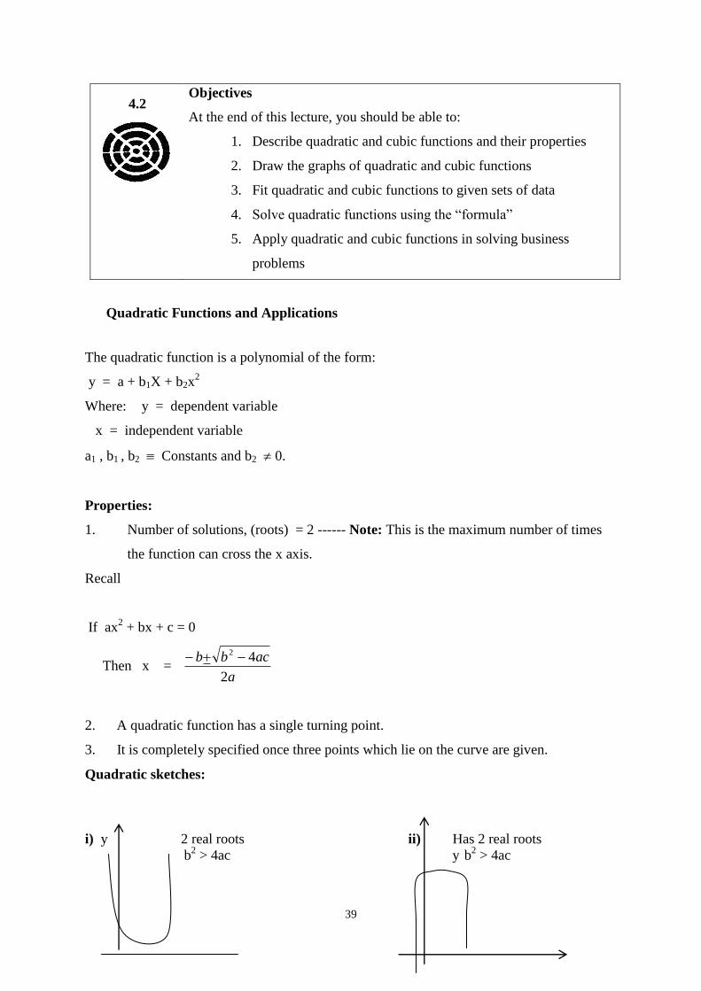
Objectives

At the end of this lecture, you should be able to:

1. Describe quadratic and cubic functions and their properties

2. Draw the graphs of quadratic and cubic functions

3. Fit quadratic and cubic functions to given sets of data

4. Solve quadratic functions using the “formula”

5. Apply quadratic and cubic functions in solving business

problems

Quadratic Functions and Applications

The quadratic function is a polynomial of the form:

y = a + b1X + b2x2

Where: y = dependent variable

x = independent variable

a1 , b1 , b2 Constants and b2 0.

Properties:

1. Number of solutions, (roots) = 2 ------ Note: This is the maximum number of times

the function can cross the x axis.

Recall

If ax2 + bx + c = 0

Then x = a

acbb

2

42

2. A quadratic function has a single turning point.

3. It is completely specified once three points which lie on the curve are given.

Quadratic sketches:

i) y 2 real roots ii) Has 2 real roots

b2 > 4ac y b

2 > 4ac

4.2

40

x x

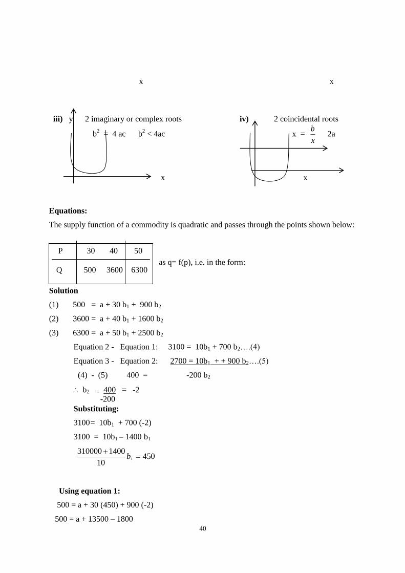
iii) y 2 imaginary or complex roots iv) 2 coincidental roots

b2 = 4 ac b

2 < 4ac x =

x

b 2a

x x

Equations:

The supply function of a commodity is quadratic and passes through the points shown below:

Determine the supply function as q= f(p), i.e. in the form:

q = a + b1 p + b2p2

Solution

(1) 500 = a + 30 b1 + 900 b2

(2) 3600 = a + 40 b1 + 1600 b2

(3) 6300 = a + 50 b1 + 2500 b2

Equation 2 - Equation 1: 3100 = 10b1 + 700 b2….(4)

Equation 3 - Equation 2: 2700 = 10b1 + + 900 b2….(5)

(4) - (5) 400 = -200 b2

b2 = 400 = -2

-200

Substituting:

3100 = 10b1 + 700 (-2)

3100 = 10b1 – 1400 b1

45010

14003100001

b

Using equation 1:

500 = a + 30 (450) + 900 (-2)

500 = a + 13500 – 1800

P 30 40 50

Q 500 3600 6300

41

a = 500 – 13500 + 1800

a = -11,200,

Thus the Supply function is

q = -11200 + 450 p – 2p2

Example;

The demand function of a certain commodity is quadratic and passes through the points

(p,q)= (5,1600); (10,900); (20,100);

Determine the function in form; q = a + b1 p + b2p2

Solution:

q = a + b1 p + b2p

Equations

(1) 1600 = a + 5b1 + 25b2

(2) 900 = a + 10b1 + 100b2

(3) 100 = a + 20b1 + 400b2

(4) = (1) – (2): 700 = -5b1 – 75 b2

(5) = (2) – (3): = 800 = -10b1 – 300 b2

2: 400 = -5b1 – 150b2

2: = (4) – (6): 300 = 75b2

b2 = 300/75 = 4

Substituting in equation (4):

700 = -5b1 – 75(4) 700 = -5b1 – 300

b1 = 700 + 300 = -200 ; b = -5

Using equation 1

1600 = a + 5 (-200) + 25(4)

1600 = a – 1000 + 100

a = 1600 + 1000 – 100

a = 2500

Thus, the Demand function is:

q = 2500 – 200p + 4p2

42

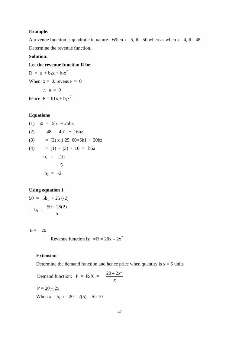
Example:

A revenue function is quadratic in nature. When x= 5, R= 50 whereas when x= 4, R= 48.

Determine the revenue function.

Solution:

Let the revenue function R be:

R = a + b1x + b2x2

When x = 0, revenue = 0

a = 0

hence R = b1x + b2x2

Equations

(1) 50 = 5b1 + 25bz

(2) 48 = 4b1 + 16bz

(3) = (2) x 1.25 60=5b1 + 20bz

(4) = (1) - (3) - 10 = b5a

b2 = -10

5

b2 = -2.

Using equation 1

50 = 5b1 + 25 (-2)

b1 = 5

)2(2550

B = 20

Revenue function is: = R = 20x – 2x2

Extension:

Determine the demand function and hence price when quantity is x = 5 units

Demand function: P = R/X = x

x 2220

P = 20 – 2x

When x = 5, p = 20 – 2(5) = Sh 10

43

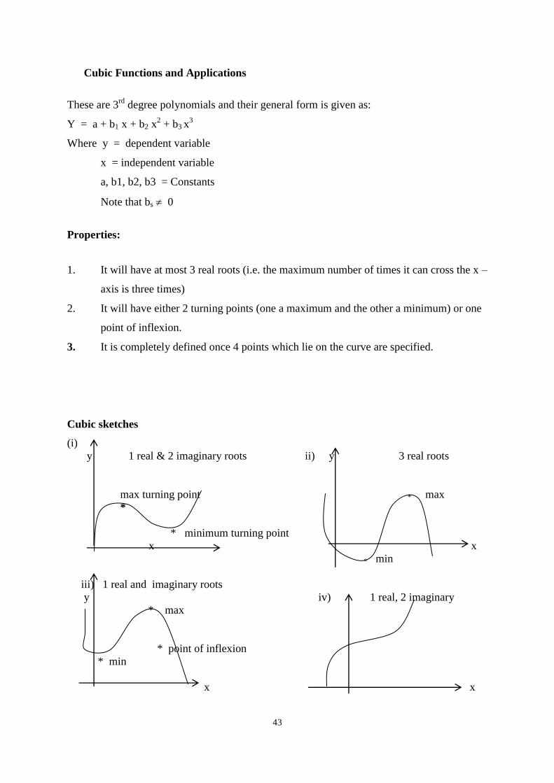
Cubic Functions and Applications

These are 3rd

degree polynomials and their general form is given as:

Y = a + b1 x + b2 x2 + b3 x

3

Where y = dependent variable

x = independent variable

a, b1, b2, b3 = Constants

Note that bs 0

Properties:

1. It will have at most 3 real roots (i.e. the maximum number of times it can cross the x –

axis is three times)

2. It will have either 2 turning points (one a maximum and the other a minimum) or one

point of inflexion.

3. It is completely defined once 4 points which lie on the curve are specified.

Cubic sketches

(i)

y 1 real & 2 imaginary roots ii) y 3 real roots

max turning point * max

*

* minimum turning point

x x

* min

iii) 1 real and imaginary roots

y iv) 1 real, 2 imaginary

* max

* point of inflexion

* min

x x

44

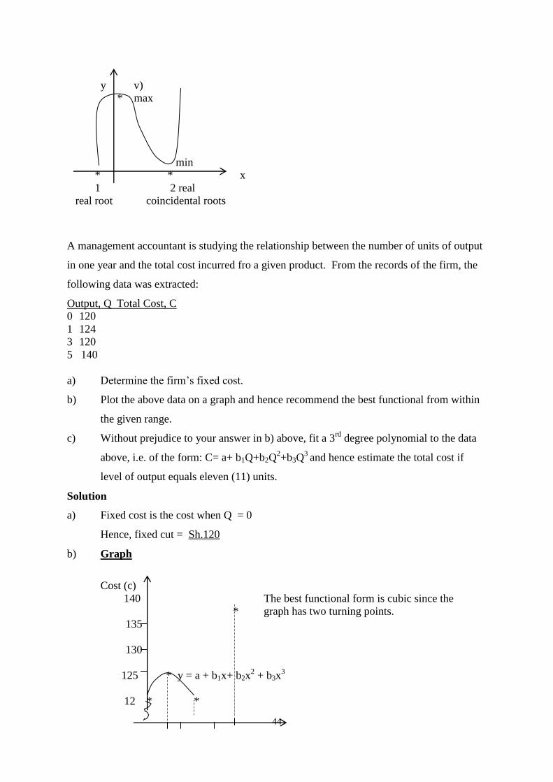
y v)

* max

min

* * x

1 2 real

real root coincidental roots

A management accountant is studying the relationship between the number of units of output

in one year and the total cost incurred fro a given product. From the records of the firm, the

following data was extracted:

Output, Q Total Cost, C

0 120

1 124

3 120

5 140

a) Determine the firm’s fixed cost.

b) Plot the above data on a graph and hence recommend the best functional from within

the given range.

c) Without prejudice to your answer in b) above, fit a 3rd

degree polynomial to the data

above, i.e. of the form: C= a+ b1Q+b2Q2+b3Q

3 and hence estimate the total cost if

level of output equals eleven (11) units.

Solution

a) Fixed cost is the cost when Q = 0

Hence, fixed cut = Sh.120

b) Graph

Cost (c)

140 The best functional form is cubic since the

* graph has two turning points.

135

130

125 * y = a + b1x+ b2x2 + b3x

3

12 * *

45

0 1 2 3 4 5 Q

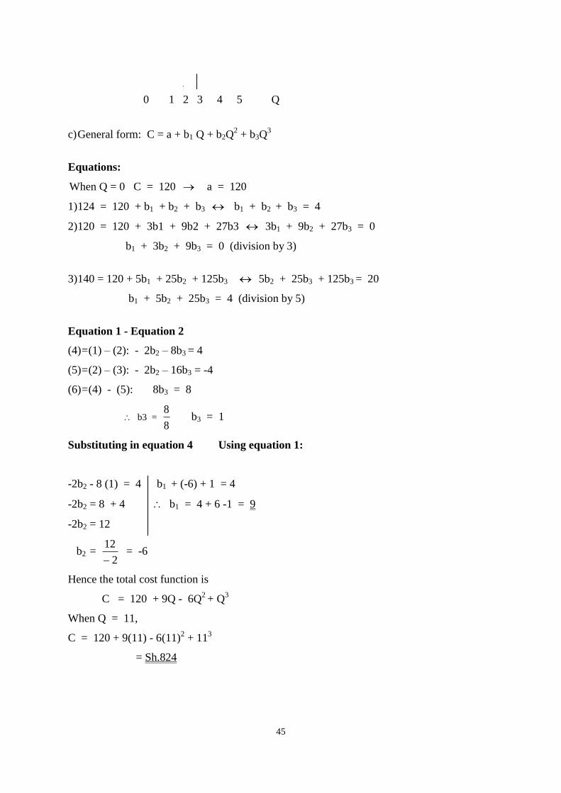
c) General form: C = a + b1 Q + b2Q2 + b3Q

3

Equations:

When Q = 0 C = 120 a = 120

1) 124 = 120 + b1 + b2 + b3 b1 + b2 + b3 = 4

2) 120 = 120 + 3b1 + 9b2 + 27b3 3b1 + 9b2 + 27b3 = 0

b1 + 3b2 + 9b3 = 0 (division by 3)

3) 140 = 120 + 5b1 + 25b2 + 125b3 5b2 + 25b3 + 125b3 = 20

b1 + 5b2 + 25b3 = 4 (division by 5)

Equation 1 - Equation 2

(4) = (1) – (2): - 2b2 – 8b3 = 4

(5) = (2) – (3): - 2b2 – 16b3 = -4

(6) = (4) - (5): 8b3 = 8

b3 = 8

8 b3 = 1

Substituting in equation 4 Using equation 1:

-2b2 - 8 (1) = 4 b1 + (-6) + 1 = 4

-2b2 = 8 + 4 b1 = 4 + 6 -1 = 9

-2b2 = 12

b2 = 2

12

= -6

Hence the total cost function is

C = 120 + 9Q - 6Q2

+ Q3

When Q = 11,

C = 120 + 9(11) - 6(11)2 + 11

3

= Sh.824

46

4.5

Summary

In this lecture, we have looked at quadratic and cubic functions. We have

studied their properties, how to get their equations and how to sketch their

graphs. We have also looked at the importance and application of these

functions in solving business problems. In the next lecture, you will study

multivariate, exponential and logarithmic functions.

Activity 4.1

Sosina Ltd. specializes in renting out a certain type of equipment. In their planning

Endeavour, they have invited you to analyze the relationship between profit and the number

of units of the equipment rented out. You obtain the following data from their records:

Number of units rented out per day Total Daily profit ($)

20 60

30 110

40 140

Further, the firm does not rent out more than 100 units daily and within this relevant range

(i.e. 0 – 100) , you think that a quadratic model is the most suitable.

Required:

(a) Determine the function relating daily profit to the number of units rented out.

(b) From the function above, determine the daily level of fixed cost and the average daily

profit per unit of equipment.

47

(c) At what level of equipment rental are total daily profit equal to zero (i.e. the break even

point)?

(d) Determine the level of equipment to be rented out per day that maximizes daily profit

and this profit.

48

LECTURE FIVE

MULTIVARIATE, EXPONENTIAL AND LOGARITHMIC FUNCTIONS

Lecture Outlines

5.1 Introduction

5.2 Objectives

5.3 Multivariate Functions

5.4 Exponential Functions

5.5 Modified Exponential Functions

5.6 Logarithmic Functions

5.6.1 Properties of Logarithms

5.6.2 Solving Logarithmic Exponential Equations

5.6.3 Application of Exponential & Logarithmic Functions

5.7 Summary

5.1 Introduction

Welcome to lecture five. We are still studying functions. In this lecture, we shall study

functions which have more than one independent variables (multivariate functions) and

functions which are quite useful in describing growth and decay phenomena (exponential and

logarithmic functions).

Objectives

At the end of this lecture, you should be able to:

1. Describe and apply multivariate functions.

2. Identify and sketch general exponential and logarithmic

functions.

3. Solve simple exponential and logarithmic equations.

4. Use the exponential functions to model growth and decay

processes.

5.3 Multivariate Functions

In business, there are many dependent variables of interest which are determined by two or

more independent variables, for example:

Savings can be determined by income, household size and interest rates;

Sales level can be determined by level of advertisement and prices of related goods

and so on. These are known as multivariate functions.

5.2

49

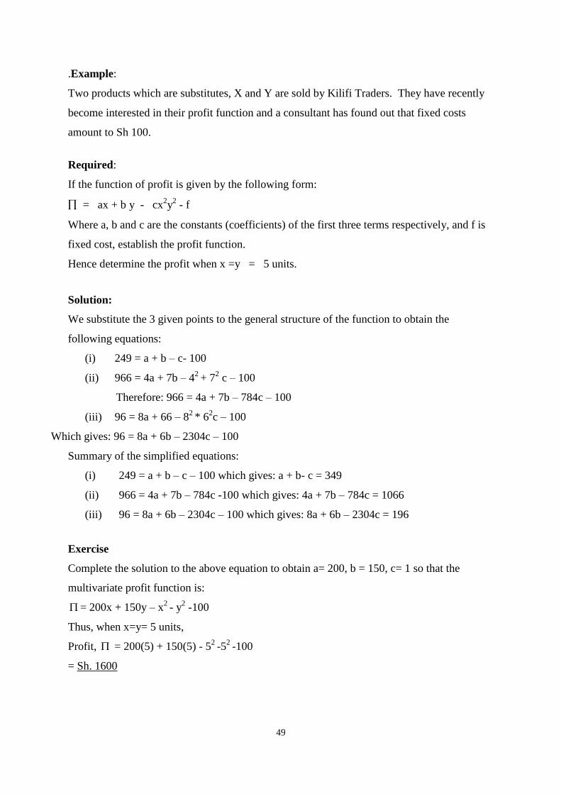
.Example:

Two products which are substitutes, X and Y are sold by Kilifi Traders. They have recently

become interested in their profit function and a consultant has found out that fixed costs

amount to Sh 100.

Required:

If the function of profit is given by the following form:

= ax + b y - cx2y

2 - f

Where a, b and c are the constants (coefficients) of the first three terms respectively, and f is

fixed cost, establish the profit function.

Hence determine the profit when x =y = 5 units.

Solution:

We substitute the 3 given points to the general structure of the function to obtain the

following equations:

(i) 249 = a + b – c- 100

(ii) 966 = 4a + 7b – 42

+ 72 c – 100

Therefore: 966 = 4a + 7b – 784c – 100

(iii) 96 = 8a + 66 – 82

* 62c – 100

Which gives: 96 = 8a + 6b – 2304c – 100

Summary of the simplified equations:

(i) 249 = a + b – c – 100 which gives: a + b- c = 349

(ii) 966 = 4a + 7b – 784c -100 which gives: 4a + 7b – 784c = 1066

(iii) 96 = 8a + 6b – 2304c – 100 which gives: 8a + 6b – 2304c = 196

Exercise

Complete the solution to the above equation to obtain a= 200, b = 150, c= 1 so that the

multivariate profit function is:

= 200x + 150y – x2

- y2 -100

Thus, when x=y= 5 units,

Profit, = 200(5) + 150(5) - 52

-52

-100

= Sh. 1600

50

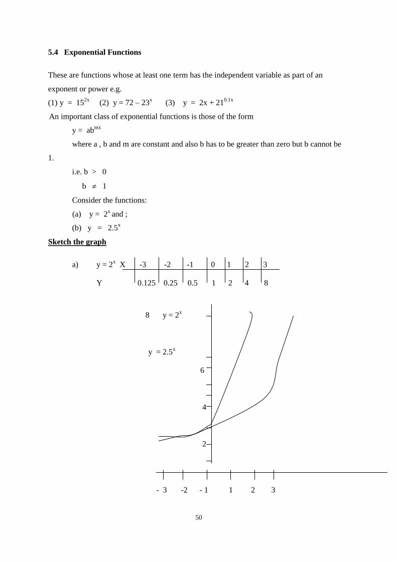
5.4 Exponential Functions

These are functions whose at least one term has the independent variable as part of an

exponent or power e.g.

(1) y = 152x

(2) y = 72 – 23x (3)

y = 2x + 21

0.1x

An important class of exponential functions is those of the form

y = abmx

where a , b and m are constant and also b has to be greater than zero but b cannot be

1.

i.e. b > 0

b 1

Consider the functions:

(a) y = 2x and ;

(b) y = 2.5x

Sketch the graph

a) y = 2x X -3 -2 -1 0 1 2 3

Y 0.125 0.25 0.5 1 2 4 8

8 y = 2x

y = 2.5x

6

4

2

- 3 -2 - 1 1 2 3

51

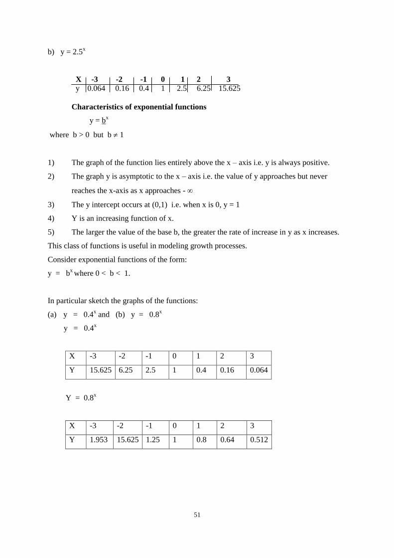
b) y = 2.5x

X -3 -2 -1 0 1 2 3

y 0.064 0.16 0.4 1 2.5 6.25 15.625

Characteristics of exponential functions

y = bx

where b > 0 but b 1

1) The graph of the function lies entirely above the x – axis i.e. y is always positive.

2) The graph y is asymptotic to the x – axis i.e. the value of y approaches but never

reaches the x-axis as x approaches -

3) The y intercept occurs at (0,1) i.e. when x is 0, y = 1

4) Y is an increasing function of x.

5) The larger the value of the base b, the greater the rate of increase in y as x increases.

This class of functions is useful in modeling growth processes.

Consider exponential functions of the form:

y = bx where 0 < b < 1.

In particular sketch the graphs of the functions:

(a) y = 0.4x and (b) y = 0.8

x

y = 0.4x

X -3 -2 -1 0 1 2 3

Y 15.625 6.25 2.5 1 0.4 0.16 0.064

Y = 0.8x

X -3 -2 -1 0 1 2 3

Y 1.953 15.625 1.25 1 0.8 0.64 0.512

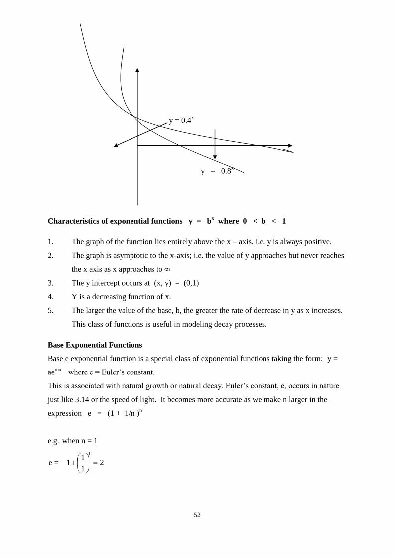
52

y = 0.4x

y = 0.8x

Characteristics of exponential functions y = bx where 0 < b < 1

1. The graph of the function lies entirely above the x – axis, i.e. y is always positive.

2. The graph is asymptotic to the x-axis; i.e. the value of y approaches but never reaches

the x axis as x approaches to ∞

3. The y intercept occurs at (x, y) = (0,1)

4. Y is a decreasing function of x.

5. The larger the value of the base, b, the greater the rate of decrease in y as x increases.

This class of functions is useful in modeling decay processes.

Base Exponential Functions

Base e exponential function is a special class of exponential functions taking the form: y =

aemx

where e = Euler’s constant.

This is associated with natural growth or natural decay. Euler’s constant, e, occurs in nature

just like 3.14 or the speed of light. It becomes more accurate as we make n larger in the

expression e = (1 + 1/n )n

e.g. when n = 1

e = 21

11

1

53

when n = 2

e = 25.22

11

2

when n = 10

e = 5937.210

11

2

when n = 50

e = 691.250

11

10

when n = 100

e = 7048.2100

11

100

when n = 1000

e = 7169.21000

11

1000

From a calculator, the value of e is obtained by raising e to power 1 in the function ex, to four

decimal places, e1 = e = 2.7183

Activity 5.1

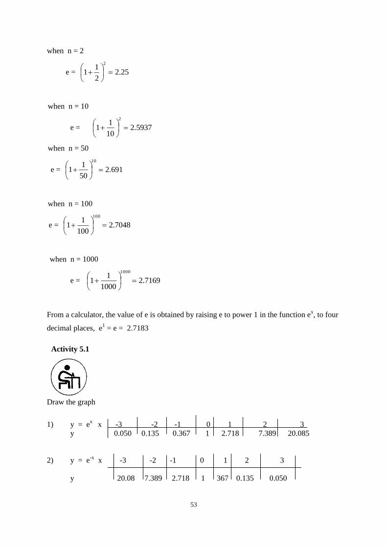
Draw the graph

1) y = ex x -3 -2 -1 0 1 2 3

y 0.050 0.135 0.367 1 2.718 7.389 20.085

2) y = e-x

x -3 -2 -1 0 1 2 3

y 20.08 7.389 2.718 1 367 0.135 0.050

54

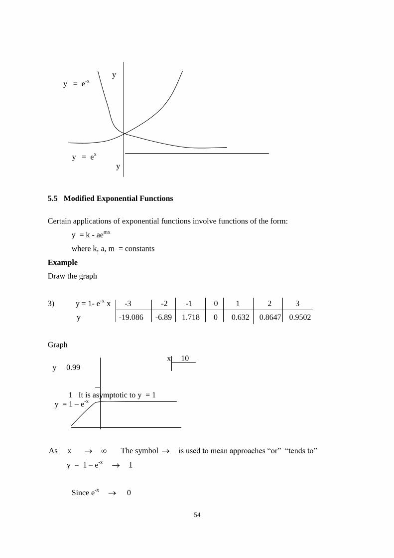
y

y = e-x

y = ex

y

5.5 Modified Exponential Functions

Certain applications of exponential functions involve functions of the form:

y = k - aemx

where k, a, m = constants

Example

Draw the graph

3) y = 1- e-x

x -3 -2 -1 0 1 2 3

y -19.086 -6.89 1.718 0 0.632 0.8647 0.9502

Graph

x 10

y 0.99

1 It is asymptotic to y = 1

y = 1 – e-x

As x The symbol is used to mean approaches “or” “tends to”

y = 1 – e-x

1

Since e-x

0

55

Applications of Exponential functions

Areas of Use

- Growth processes in business increase;

- Population growth;

- Appreciation in the value of assets,

- Inflation growth;

- Rate at which particular resources are used (e.g. demand for energy), growth in GNP

(Gross Net Product, etc.

Decay processes

Examples of decay processes are: Declining value of assets e.g. motor vehicles

(depreciation), decline in the incidences of certain decreases as medical research advances,

decrease in the purchasing power of the shilling etc.

When a growth process is characterized by a constant percentage increase in value it is

referred to as exponential growth process and when it is characterized by a constant percent

decrease. It is referred to as an exponential decay process.

Although exponential decay and growth functions are usually stated as functions of time, the

independent variable may represent something other than time.

Regardless of the nature of the independent variable, the effect is that equal increases in the

independent variable result in constant percent changes (increases or decreases) in the value

of dependent variable

Illustration

1. Population growth

The population of a country was 100 million in 1990. It has grown since that time at

4% p.a and the growth is exponential.

Required

(a) What is the function which describes population growth through time?

i.e. P = f (t)?

b) What is the population in year 2010?

56

Solution

(a) The function is:

y = ae kt

where a y when t = 0

k decay or growth rate

1990

t = 0

k 0.04

P = 100e0.04t

(b) In 2010: t = 2010 – 1990 t = 20 years.

P = 100e0.04 x 20

p = 100e0.8

= 222.5541 million

1. Asset valuation

The depreciation function, V, of a certain piece of industrial equipment has been

found to be described by the function:

V = 100e –0.1t

Where t time in years

V = book value at time t

Required:

a) What is the annual depreciation rate?

b) What was the purchase cost of the asset?

c) What is the book value after

i) 6 years?

ii) 11 years?

Solution

a) Annual depreciation rate is 10%

b) V = 100e0 = 100,000

c) i) V = 100e –0.1 x 6

= 100e-0.6

= Sh 54,881

ii) V = 100e –0.1 x 12

V = 30,120

57

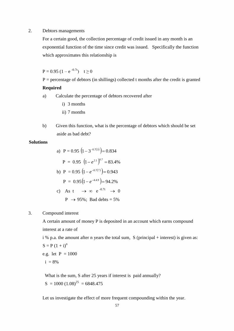
2. Debtors managements

For a certain good, the collection percentage of credit issued in any month is an

exponential function of the time since credit was issued. Specifically the function

which approximates this relationship is

P = 0.95 (1 – e -0.7t

) t ≥ 0

P = percentage of debtors (in shillings) collected t months after the credit is granted

Required

a) Calculate the percentage of debtors recovered after

i) 3 months

ii) 7 months

b) Given this function, what is the percentage of debtors which should be set

aside as bad debt?

Solutions

a) P = 0.95 834.031 37.0

P = 0.95 %4.8317.01.2 e

b) P = 0.95 943.01 77.0 e

P = 0.95 %2.941 9.4.4 e

c) As t e -0.7t

0

P 95%; Bad debts = 5%

3. Compound interest

A certain amount of money P is deposited in an account which earns compound

interest at a rate of

i % p.a. the amount after n years the total sum, S (principal + interest) is given as:

S = P (1 + i)n

e.g. let P = 1000

i = 8%

What is the sum, S after 25 years if interest is paid annually?

S = 1000 (1.08)25

= 6848.475

Let us investigate the effect of more frequent compounding within the year.

58

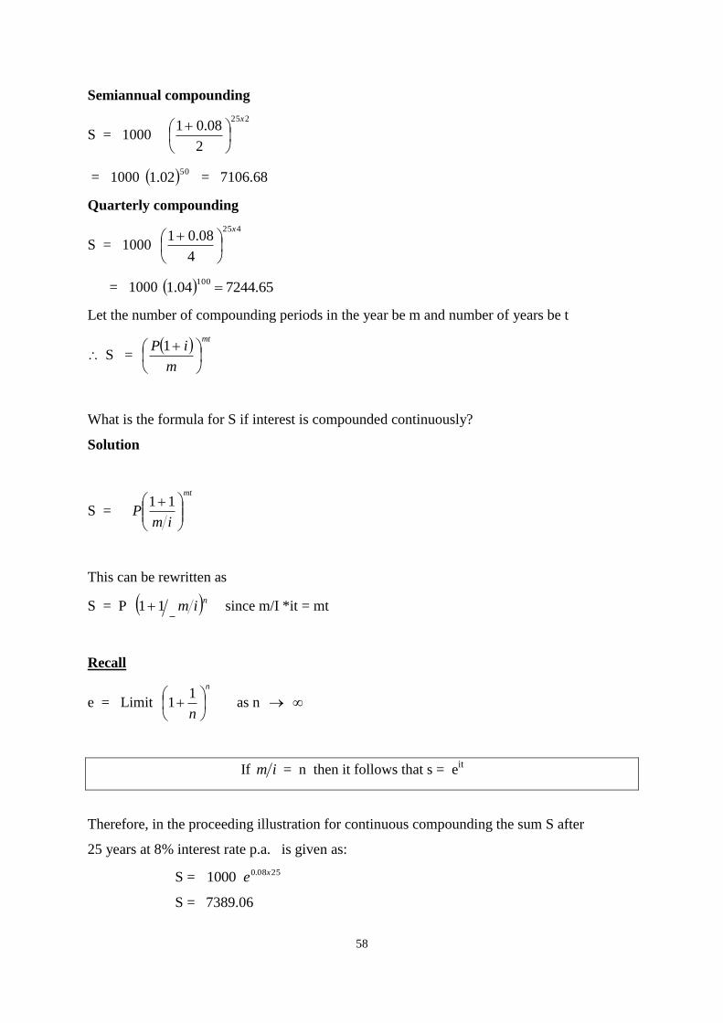
Semiannual compounding

S = 1000

225

2

08.01x

= 1000 5002.1 = 7106.68

Quarterly compounding

S = 1000

425

4

08.01x

= 1000 65.724404.1100

Let the number of compounding periods in the year be m and number of years be t

S = mt

m

iP

1

What is the formula for S if interest is compounded continuously?

Solution

S =

mt

imP

11

This can be rewritten as

S = P nim11 since m/I *it = mt

Recall

e = Limit

n

n

11

as n ∞

If im = n then it follows that s = eit

Therefore, in the proceeding illustration for continuous compounding the sum S after

25 years at 8% interest rate p.a. is given as:

S = 1000 2508.0 xe

S = 7389.06

59

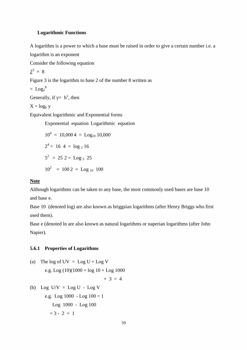
Logarithmic Functions

A logarithm is a power to which a base must be raised in order to give a certain number i.e. a

logarithm is an exponent

Consider the following equation

23 = 8

Figure 3 is the logarithm to base 2 of the number 8 written as

= Log28

Generally, if y= bx, then

X = logb y

Equivalent logarithmic and Exponential forms

Exponential equation Logarithmic equation

104 = 10,000 4 = Log10 10,000

24 = 16 4 = log 2 16

52

= 25 2 = Log 5 25

102 = 100 2 = Log 10 100

Note

Although logarithms can be taken to any base, the most commonly used bases are base 10

and base e.

Base 10 (denoted log) are also known as briggsian logarithms (after Henry Briggs who first

used them).

Base e (denoted ln are also known as natural logarithms or naperian logarithms (after John

Napier).

5.6.1 Properties of Logarithms

(a) The log of UV = Log U + Log V

e.g. Log (10)(1000 = log 10 + Log 1000

+ 3 = 4

(b) Log U/V = Log U - Log V

e.g. Log 1000 - Log 100 = 1

Log 1000 - Log 100

= 3 - 2 = 1

60

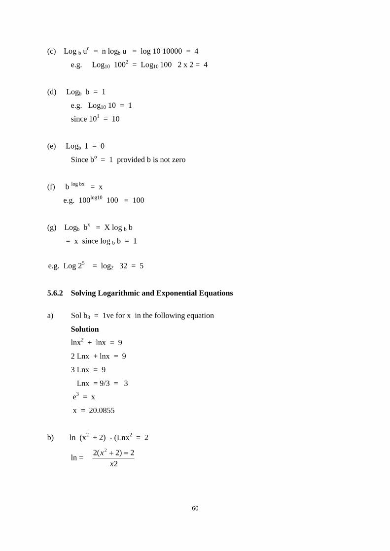
(c) Log b un = n logb u = log 10 10000 = 4

e.g. Log10 1002 = Log10 100 2 x 2 = 4

(d) Logb b = 1

e.g. Log10 10 = 1

since 101 = 10

(e) Logb 1 = 0

Since bo = 1 provided b is not zero

(f) b log bx

= x

e.g. 100log10

100 = 100

(g) Logb bx = X log b b

= x since log b b = 1

e.g. Log 25 = log2 32 = 5

5.6.2 Solving Logarithmic and Exponential Equations

a) Sol b3 = 1ve for x in the following equation

Solution

lnx2 + lnx = 9

2 Lnx + lnx = 9

3 Lnx = 9

Lnx = 9/3 = 3

e3 = x

x = 20.0855

b) ln (x2 + 2) - (Lnx

2 = 2

ln = 2

2)2(2 2

x

x

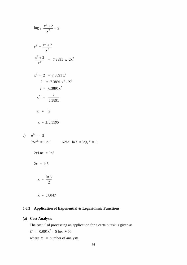
61

log e 22

2

2

x

x

e2 =

2

2 2

x

x

2

2 2

x

x = 7.3891 x 2x

2

x2 + 2 = 7.3891 x

2

2 = 7.3891 x2

- X2

2 = 6.3891x2

x2 =

3891.6

2

x = 2

x = 0.5595

c) e2x

= 5

lne2x

= Ln5 Note ln e = loge e = 1

2xLne = ln5

2x = ln5

x = 2

5ln

x = 0.8047

5.6.3 Application of Exponential & Logarithmic Functions

(a) Cost Analysis

The cost C of processing an application for a certain task is given as

C = 0.001x2 - 5 lnx + 60

where x = number of analysts

62

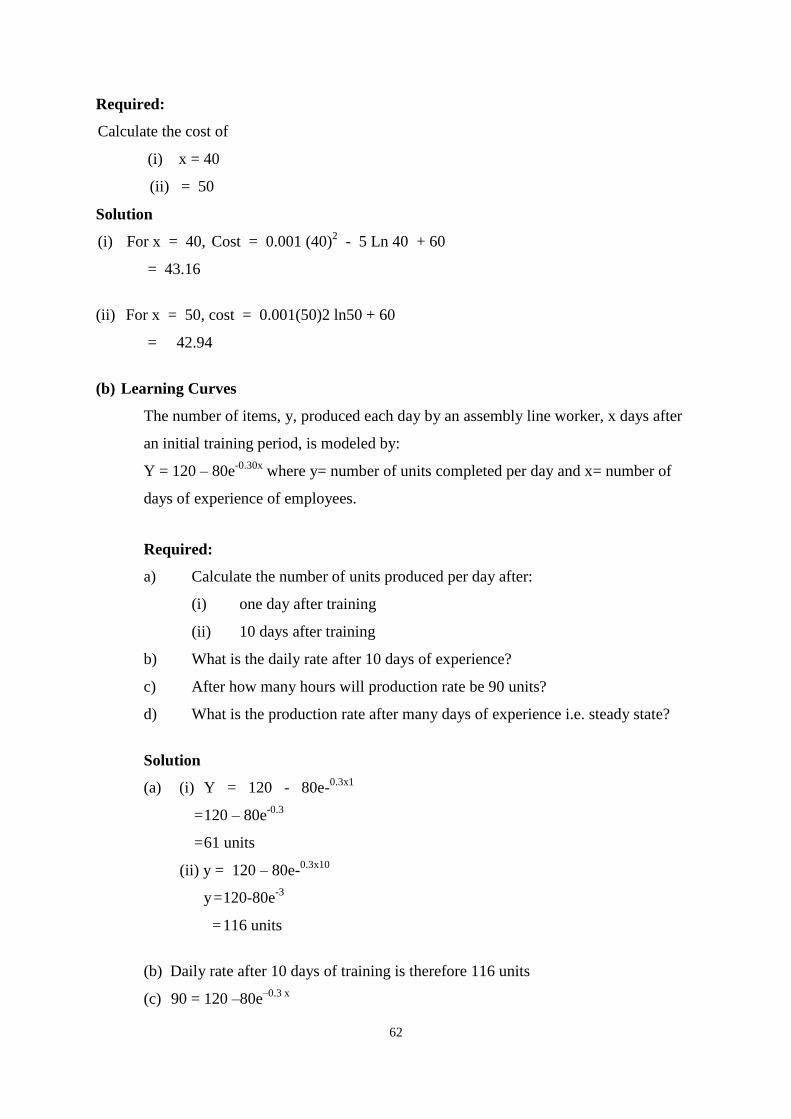
Required:

Calculate the cost of

(i) x = 40

(ii) = 50

Solution

(i) For x = 40, Cost = 0.001 (40)2 - 5 Ln 40 + 60

= 43.16

(ii) For x = 50, cost = 0.001(50)2 ln50 + 60

= 42.94

(b) Learning Curves

The number of items, y, produced each day by an assembly line worker, x days after

an initial training period, is modeled by:

Y = 120 – 80e-0.30x

where y= number of units completed per day and x= number of

days of experience of employees.

Required:

a) Calculate the number of units produced per day after:

(i) one day after training

(ii) 10 days after training

b) What is the daily rate after 10 days of experience?

c) After how many hours will production rate be 90 units?

d) What is the production rate after many days of experience i.e. steady state?

Solution

(a) (i) Y = 120 - 80e-0.3x1

= 120 – 80e-0.3

= 61 units

(ii) y = 120 – 80e-0.3x10

y = 120-80e-3

= 116 units

(b) Daily rate after 10 days of training is therefore 116 units

(c) 90 = 120 –80e–0.3 x

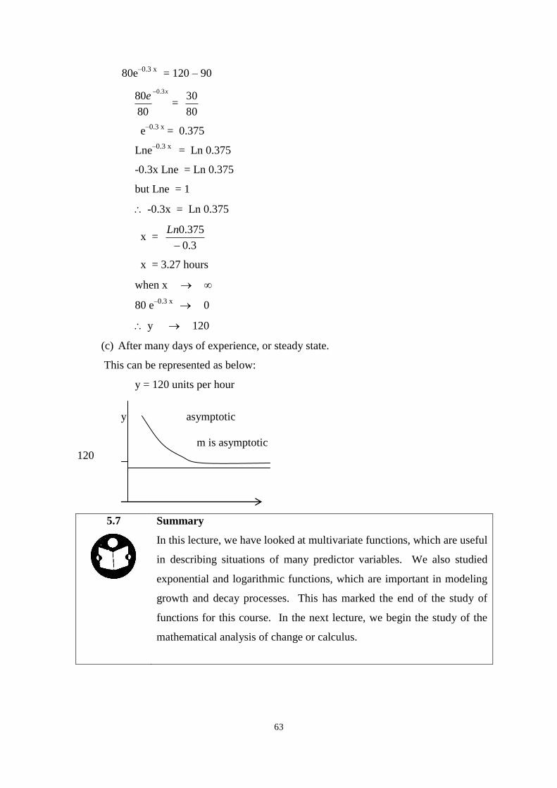
63

80e–0.3 x

= 120 – 90

xe

3.0

80

80

= 80

30

e–0.3 x

= 0.375

Lne–0.3 x

= Ln 0.375

-0.3x Lne = Ln 0.375

but Lne = 1

-0.3x = Ln 0.375

x = 3.0

375.0

Ln

x = 3.27 hours

when x

80 e–0.3 x

0

y 120

(c) After many days of experience, or steady state.

This can be represented as below:

y = 120 units per hour

y asymptotic

m is asymptotic

120

5.7

Summary

In this lecture, we have looked at multivariate functions, which are useful

in describing situations of many predictor variables. We also studied

exponential and logarithmic functions, which are important in modeling

growth and decay processes. This has marked the end of the study of

functions for this course. In the next lecture, we begin the study of the

mathematical analysis of change or calculus.

64

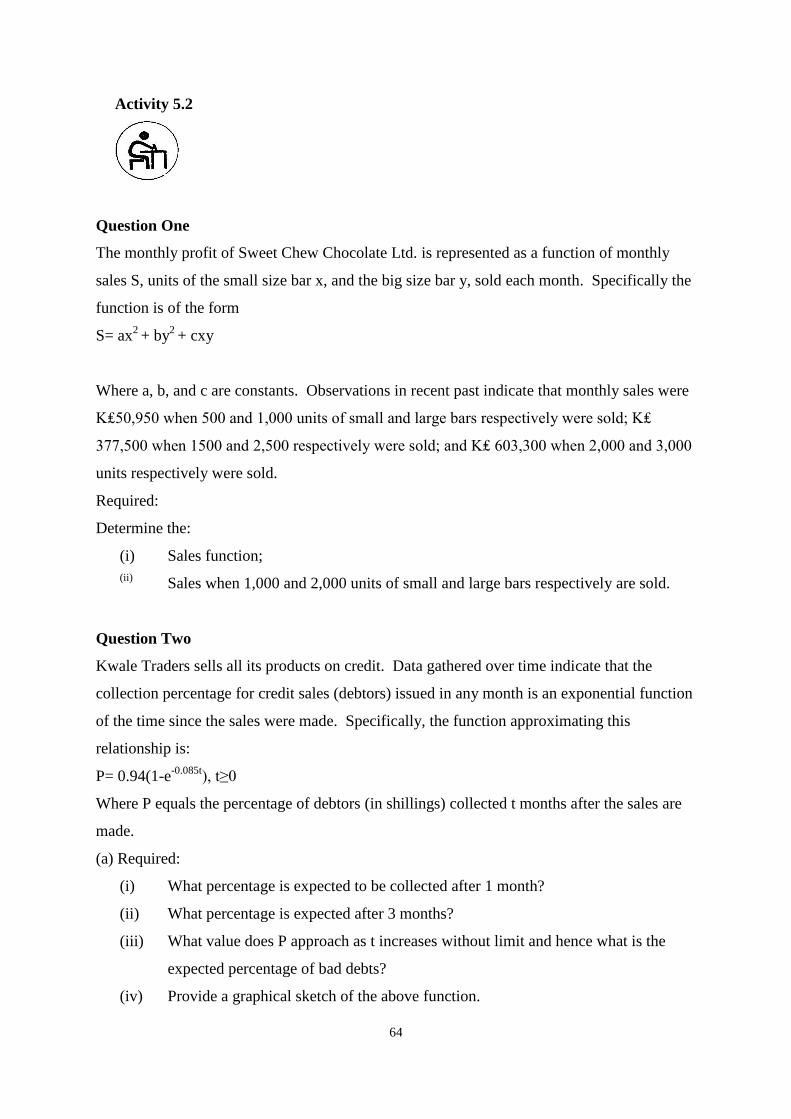
Activity 5.2

Question One

The monthly profit of Sweet Chew Chocolate Ltd. is represented as a function of monthly

sales S, units of the small size bar x, and the big size bar y, sold each month. Specifically the

function is of the form

S= ax2 + by

2 + cxy

Where a, b, and c are constants. Observations in recent past indicate that monthly sales were

K₤50,950 when 500 and 1,000 units of small and large bars respectively were sold; K₤

377,500 when 1500 and 2,500 respectively were sold; and K₤ 603,300 when 2,000 and 3,000

units respectively were sold.

Required:

Determine the:

(i) Sales function;

(ii) Sales when 1,000 and 2,000 units of small and large bars respectively are sold.

Question Two

Kwale Traders sells all its products on credit. Data gathered over time indicate that the

collection percentage for credit sales (debtors) issued in any month is an exponential function

of the time since the sales were made. Specifically, the function approximating this

relationship is:

P= 0.94(1-e-0.085t

), t≥0

Where P equals the percentage of debtors (in shillings) collected t months after the sales are

made.

(a) Required:

(i) What percentage is expected to be collected after 1 month?

(ii) What percentage is expected after 3 months?

(iii) What value does P approach as t increases without limit and hence what is the

expected percentage of bad debts?

(iv) Provide a graphical sketch of the above function.

65

(b)Twaomin Ltd is hiring persons to work in its plant. For the kind of job available, it has

been estimated by efficiency experts that the average cost, AC of performing the task is a

function of the number of persons hired, x. Specifically,

AC= 0.00005x2 – ln 2x + 6

Required:

(i) Determine the number of persons who should be hired to minimize the average

cost. Ensure it is minimum

(ii) What is the minimum average cost?

(iii) What is the minimum total cost?

Question Three

An advertising company is interested in the retention rate of a person exposed to an advert t

hours after the subject views the advert. In one such advert, subjects wee asked to look at a

picture that contained many different objects.

At different intervals after this, they would be asked to recall as many objects as they could.

Based on the experiment, the following function was developed:

R= 90- 20 ln t

Where R equals the average percentage recall and t equals time in hours since studying the

picture.

(i) Determine the recall percentage after 2 hours and after 10 hours

(ii) Determine the time when the recall percentage is 50%

(iii) At what time is the recall percentage estimated to be zero?

(iv) Provide a graphical sketch of the above function

66

LECTURE SIX

CALCULUS

Lecture Outlines

6.1 Introduction

6.2 Objectives

6.3 Importance of Calculus

6.4 Linear functions and slopes

6.5 Summary

6.1 Introduction

Welcome to Lecture Six of this course unit. In Lectures three to five, we studied

relationships between business variables which we called functions. In this lecture, we are

now concerned about how changes in independent variables affect changes in the dependent

variable.

This is important since it enables decision makers to control these changes to achieve desired

objectives. For example, how does change in output affect change in profit?

The mathematical analysis of change or movement is known as calculus.

Background

Calculus is concerned with mathematical analysis of change or movement. There are 2 basic

operations in calculus:

- Differentiation

- Integration

The two basic operations are inverse to one another as addition and subtraction or

multiplication and division.

Objectives

At the end of this lecture, you should be able to:

1. Discuss the importance of calculus in solving business

problems.

2. Distinguish between differentiation and integration.

3. Calculate and interpret the slope of a straight line.

6.2

67

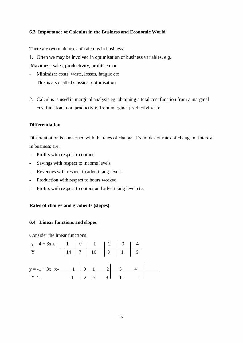
6.3 Importance of Calculus in the Business and Economic World

There are two main uses of calculus in business:

1. Often we may be involved in optimisation of business variables, e.g.

Maximize: sales, productivity, profits etc or

- Minimize: costs, waste, losses, fatigue etc

This is also called classical optimisation

2. Calculus is used in marginal analysis eg. obtaining a total cost function from a marginal

cost function, total productivity from marginal productivity etc.

Differentiation

Differentiation is concerned with the rates of change. Examples of rates of change of interest

in business are:

- Profits with respect to output

- Savings with respect to income levels

- Revenues with respect to advertising levels

- Production with respect to hours worked

- Profits with respect to output and advertising level etc.

Rates of change and gradients (slopes)

6.4 Linear functions and slopes

Consider the linear functions:

y = 4 + 3x x - 1 0 1 2 3 4

Y 14 7 10 3 1 6

y = -1 + 3x x - 1 0 1 2 3 4

Y -4 - 1 2 5 8 1 1

68

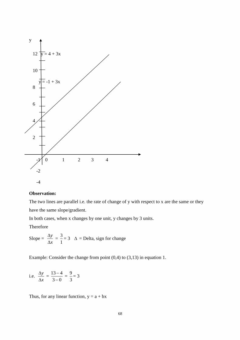
y

12 y = 4 + 3x

10

y = -1 + 3x

8

6

4

2

-1 0 1 2 3 4

-2

-4

Observation:

The two lines are parallel i.e. the rate of change of y with respect to x are the same or they

have the same slope/gradient.

In both cases, when x changes by one unit, y changes by 3 units.

Therefore

Slope = x

y

=

1

3= 3 = Delta, sign for change

Example: Consider the change from point (0,4) to (3,13) in equation 1.

i.e. x

y

=

03

413

=

3

9= 3

Thus, for any linear function, y = a + bx

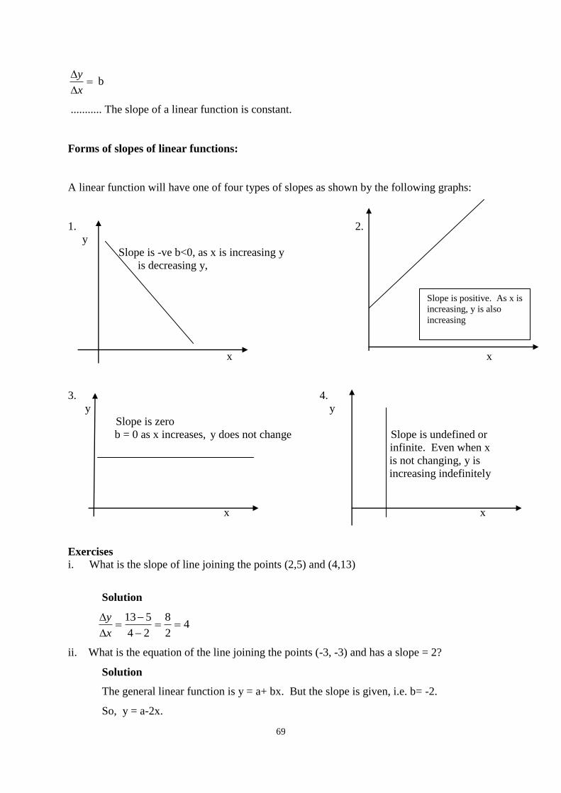
69

x

y b

........... The slope of a linear function is constant.

Forms of slopes of linear functions:

A linear function will have one of four types of slopes as shown by the following graphs:

1. 2.

y

Slope is -ve b<0, as x is increasing y

is decreasing y,

x x

3. 4.

y y

Slope is zero

b = 0 as x increases, y does not change Slope is undefined or

infinite. Even when x

is not changing, y is

increasing indefinitely

x x

Exercises

i. What is the slope of line joining the points (2,5) and (4,13)

Solution

42

8

24

513

x

y

ii. What is the equation of the line joining the points (-3, -3) and has a slope = 2?

Solution

The general linear function is y = a+ bx. But the slope is given, i.e. b= -2.

So, y = a-2x.

Slope is positive. As x is

increasing, y is also

increasing

70

To obtain the value of a, we substitute the known point as follows:

- 3= a- 2 (-3)

-3 = a +6

Therefore, a = -3 -6

a=- 9

Hence the linear function y= -9-2x.

6.5

Summary

This lecture has introduced you to calculus or the mathematical analysis of

change. We have studied the difference between differentiation and

integration and their significance in business. We have also learned how to

calculate the slope of a straight line. In the next lecture, we shall explore

how to determine slopes of non linear functions.

Activity 6.1

The demand function for a product is linear and it is of the form p = a + bq where p = price

and q = quantity. The values a and b are constants. When the price is Sh. 2, quantity

demanded is 9 units. For every increase in price by Sh. 2, quantity demanded falls by 1 unit

and vice versa.

Required:

a) Determine the demand function and hence determine the price that leads to a demand

of 4 units.

b) What price results in zero demand?

c) Determine the rate of change of price with unit with respect to quantity and interpret

it.

71

LECTURE SEVEN

GENERAL PRINCIPLES OF DIFFERENTIATION

Lecture Outlines

7.1 Introduction

7.2 Objectives

7.3 Nonlinear Functions and Slopes

7.4 Concept of Limits and Continuity

7.5 Differentiation from 1st Principles

7.6 Rules and Techniques of Differentiation

7.7 Higher order Derivatives

7.8 Summary

7.1 Introduction

Welcome to Lecture Seven of this course unit. In Lecture Six, we discussed slopes of linear

functions. Although linear functions represent many business and economic problems, there

are also many other problems which are described by non-linear functions. In this lecture, we

are concerned with slopes, or rates of change of non-linear functions.

7.2

Objectives

At the end of this lecture, you should be able to:

1. Distinguish between slope of a linear and a non-linear function.

2. Explain the concept of continuity.

3. Solve problems relating to limits.

4. Define the derivative of a function.

5. Use the rules of differentiation to find the derivatives of power

functions.

6. Obtain higher order derivatives.

7. Obtain higher order derivatives.

Non-linear functions and Slopes

The slope of a straight line is constant. However, slopes of other (non-linear) functions are

different at different points or sections of the function.

Consider the following general functions:

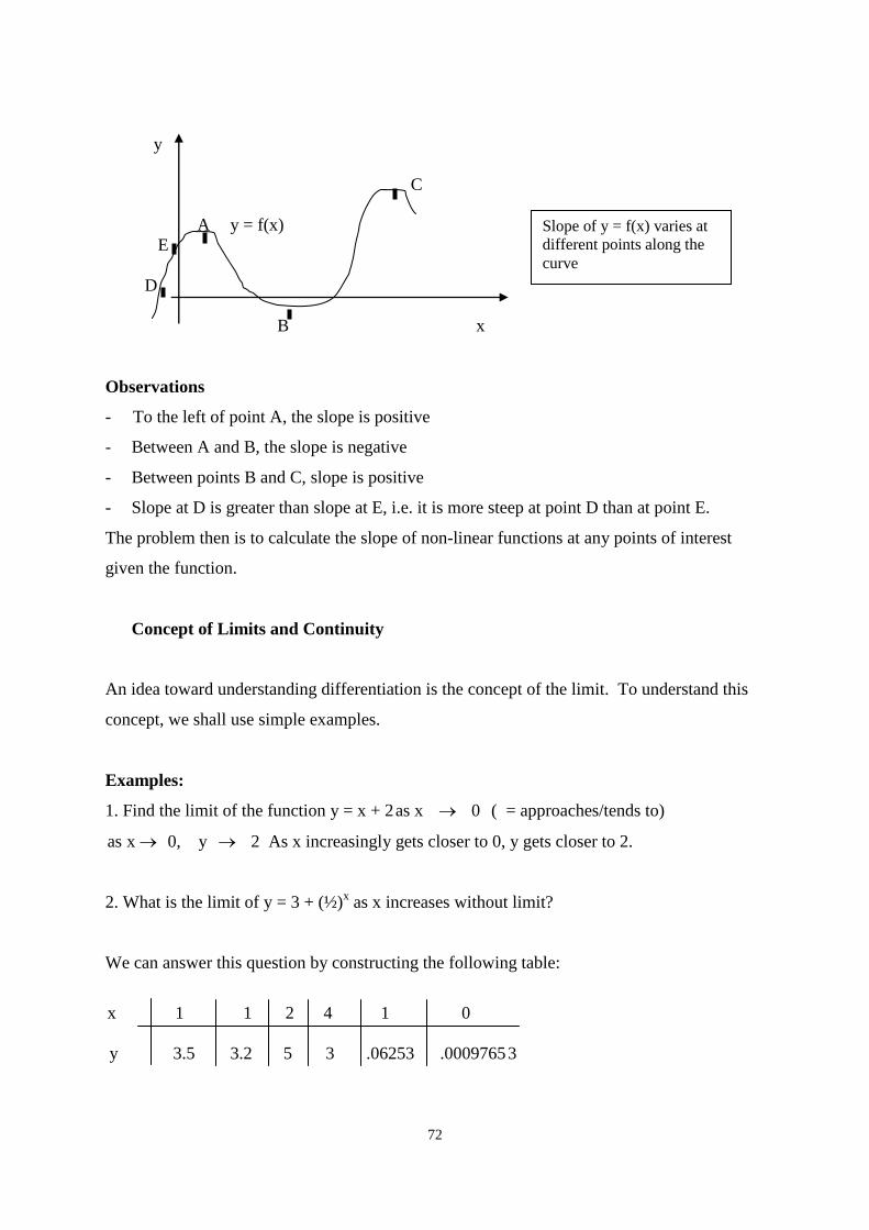
72

y

C

A y = f(x)

E

D

B x

Observations

- To the left of point A, the slope is positive

- Between A and B, the slope is negative

- Between points B and C, slope is positive

- Slope at D is greater than slope at E, i.e. it is more steep at point D than at point E.

The problem then is to calculate the slope of non-linear functions at any points of interest

given the function.

Concept of Limits and Continuity

An idea toward understanding differentiation is the concept of the limit. To understand this

concept, we shall use simple examples.

Examples:

1. Find the limit of the function y = x + 2 as x 0 ( = approaches/tends to)

as x 0, y 2 As x increasingly gets closer to 0, y gets closer to 2.

2. What is the limit of y = 3 + (½)x as x increases without limit?

We can answer this question by constructing the following table:

x 1 1 2 4 1 0

y 3.5 3.2 5 3 .06253 .0009765 3

Slope of y = f(x) varies at

different points along the

curve

73

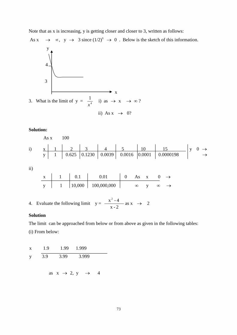
Note that as x is increasing, y is getting closer and closer to 3, written as follows:

As x , y 3 since (1/2)x 0 . Below is the sketch of this information.

y

4

3

x

3. What is the limit of y = 4

1

x i) as x ?

ii) As x 0?

Solution:

As x 100

i) x 1 2 3 4 5 10 15 y 0

y 1 0.625 0.1230 0.0039 0.0016 0.0001 0.0000198

ii)

x 1 0.1 0.01 0 As x 0

y 1 10,000 100,000,000 y

4. Evaluate the following limit y = 2-x

4 - x 2

as x 2

Solution

The limit can be approached from below or from above as given in the following tables:

(i) From below:

x 1.9 1.99 1.999

y 3.9 3.99 3.999

as x 2, y 4

74

(ii) From above

x 2.1 2.01 2.001 as x 2

y 4.1 4.01 4.001 y 4

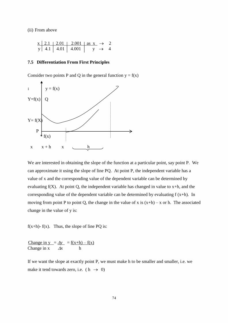
7.5 Differentiation From First Principles

Consider two points P and Q in the general function y = f(x)

: y = f(x)

Y=f(x) Q

Y= f(X)

P

* f(x)

x x + h x h

We are interested in obtaining the slope of the function at a particular point, say point P. We

can approximate it using the slope of line PQ. At point P, the independent variable has a

value of x and the corresponding value of the dependent variable can be determined by

evaluating f(X). At point Q, the independent variable has changed in value to x+h, and the

corresponding value of the dependent variable can be determined by evaluating f (x+h). In

moving from point P to point Q, the change in the value of x is (x+h) – x or h. The associated

change in the value of y is:

f(x+h)- f(x). Thus, the slope of line PQ is:

Change in y = y = f(x+h) – f(x)

Change in x x h

If we want the slope at exactly point P, we must make h to be smaller and smaller, i.e. we

make it tend towards zero, i.e. ( h 0)

75

As h tends to 0, x

y

x

y

where

x

y

is the rate of change at a point and it is also referred to as the instantaneous

rate of change. It is also called the derived function or simply the derivative.

Definition: The derivative

Given a function of the form y = f(X), the derivative of the function is:

x

y

=

h

xfhxf )()( as h 0

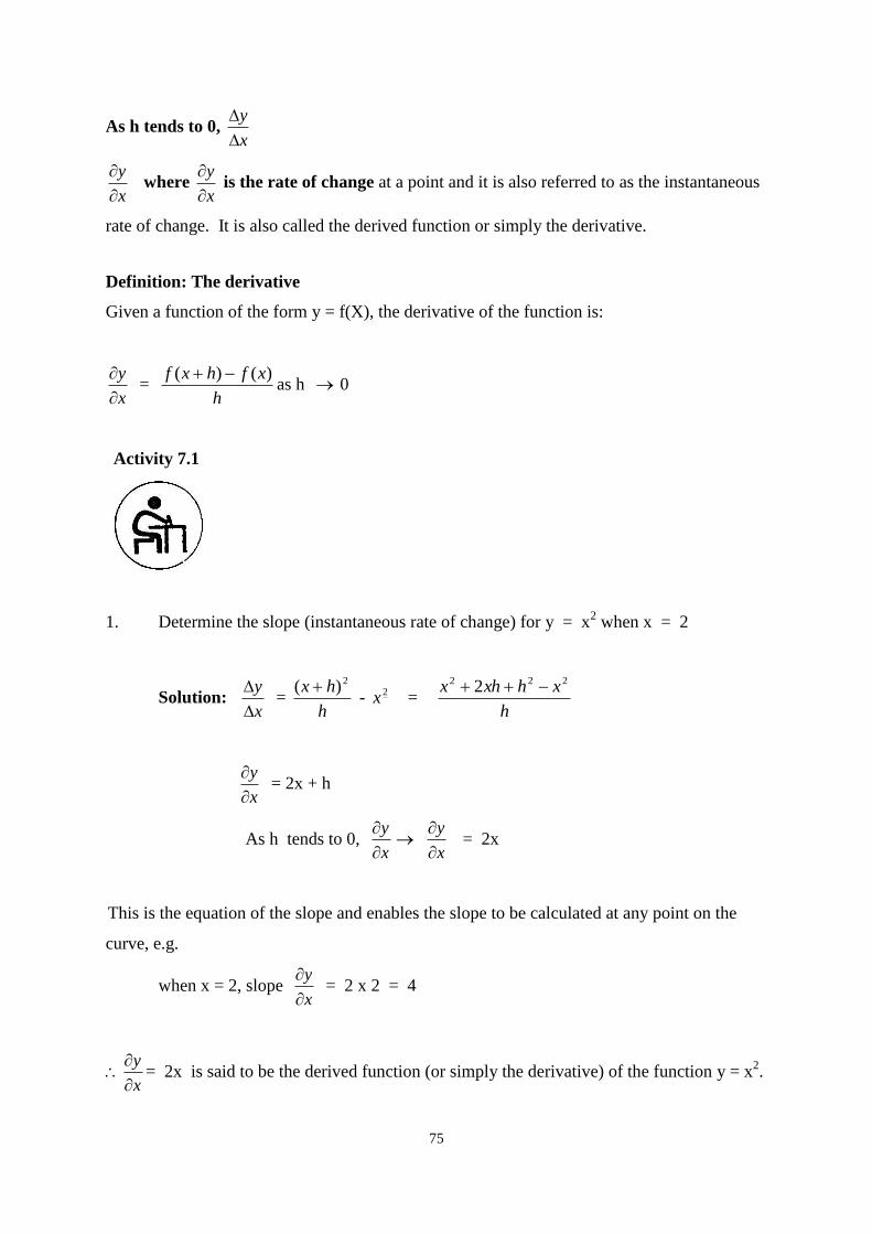
Activity 7.1

1. Determine the slope (instantaneous rate of change) for y = x2 when x = 2

Solution: x

y

=

h

hx 2)( - 2x =

h

xhxhx 222 2

x

y

= 2x + h

As h tends to 0, x

y

x

y

= 2x

This is the equation of the slope and enables the slope to be calculated at any point on the

curve, e.g.

when x = 2, slope x

y

= 2 x 2 = 4

x

y

= 2x is said to be the derived function (or simply the derivative) of the function y = x

2.

76

2. Obtain the derivative of the function

y = 4x2 - x + 3 and hence calculate the slope when x = 11

x

y

=

h

xfhxf )()( =

h

xxhxhx }34{}3)()(4{ 22

)2(4 22 hxhx

x

y

=

h

xxhxxhx 3438(4 222

x

y

= 8x + 4h - 1

As h 0 , x

y

x

y

= 8x - 1

Hence: Slope at x = 11, x

y

= 8(11) – 1 = 87

7.6 Rules and Techniques of Differentiation: (Power Functions)

Differentiation from first principles can be tedious, although it greatly assists in the

understanding of what the slope is. However, there are certain techniques for the more

commonly encountered functions which, when followed eases the task of differentiation.

These are what we study next.

1. The derivative of a constant is zero.

e.g. if y = 40, then x

y

= 0

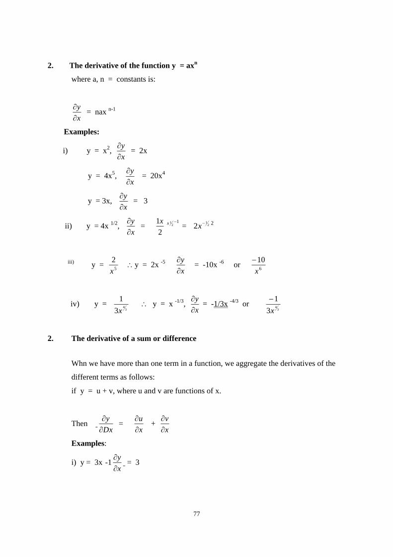
77

2. The derivative of the function y = axn

where a, n = constants is:

x

y

= nax

n-1

Examples:

i) y = x2,

x

y

= 2x

y = 4x5,

x

y

= 20x

4

y = 3x, x

y

= 3

ii) y = 4x 1/2

, x

y

=

2

1x 12

1 x = 2

1

2

x2

iii) y = 5

2

x y = 2x

-5

x

y

= -10x

-6 or

6

10

x

iv) y = 3

4

3

1

x y = x

-1/3,

x

y

= -1/3x

-4/3 or

34

3

1

x

2. The derivative of a sum or difference

Whn we have more than one term in a function, we aggregate the derivatives of the

different terms as follows:

if y = u + v, where u and v are functions of x.

Then Dx

y

=

x

u

+

x

v

Examples:

i) y = 3x -1 x

y

= 3

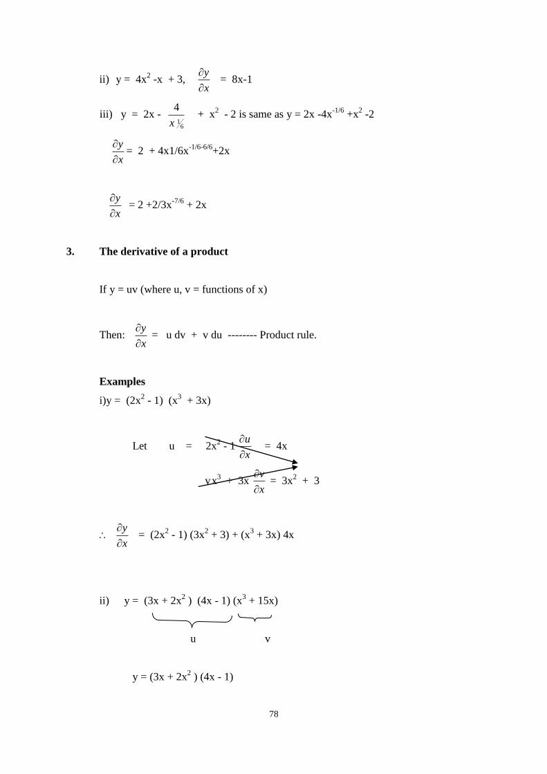
78

ii) y = 4x2 -x + 3,

x

y

= 8x-1

iii) y = 2x - 6

1

4

x + x

2 - 2 is same as y = 2x -4x

-1/6 +x

2 -2

x

y

= 2 + 4x1/6x

-1/6-6/6+2x

x

y

= 2 +2/3x

-7/6 + 2x

3. The derivative of a product

If y = uv (where u, v = functions of x)

Then: x

y

= u dv + v du -------- Product rule.

Examples

i) y = (2x2 - 1) (x

3 + 3x)

Let u = 2x2 - 1

x

u

= 4x

v x3 + 3x

x

v

= 3x

2 + 3

x

y

= (2x

2 - 1) (3x

2 + 3) + (x

3 + 3x) 4x

ii) y = (3x + 2x2 ) (4x - 1) (x

3 + 15x)

u v

y = (3x + 2x2 ) (4x - 1)

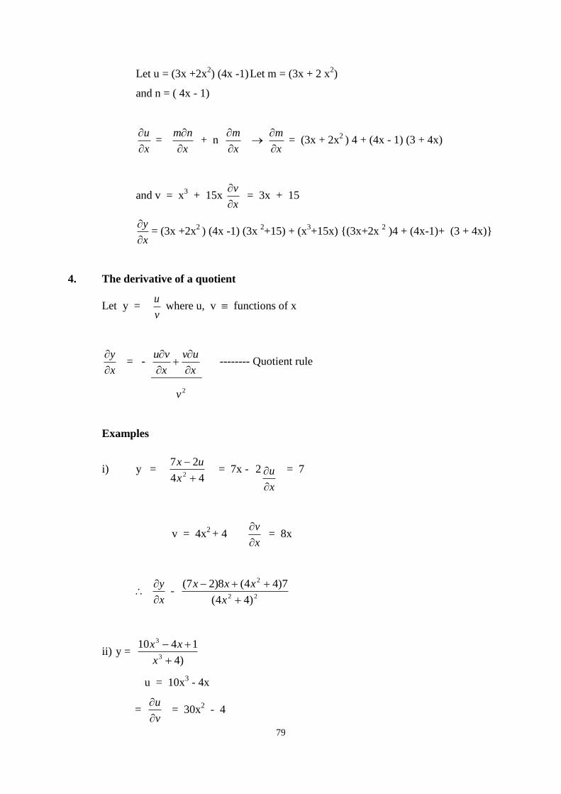
79

Let u = (3x +2x2) (4x -1) Let m = (3x + 2 x

2)

and n = ( 4x - 1)

x

u

=

x

nm

+ n

x

m

x

m

= (3x + 2x

2 ) 4 + (4x - 1) (3 + 4x)

and v = x3 + 15x

x

v

= 3x + 15

x

y

= (3x +2x

2 ) (4x -1) (3x

2+15) + (x

3+15x) {(3x+2x

2 )4 + (4x-1)+ (3 + 4x)}

4. The derivative of a quotient

Let y = v

u where u, v functions of x

x

y

= -

x

uv

x

vu

-------- Quotient rule

2v

Examples

i) y = 44

272

x

ux = 7x - 2

x

u

= 7

v = 4x2 + 4

x

v

= 8x

x

y

-

22

2

)44(

7)44(8)27(

x

xxx

ii) y = )4

14103

3

x

xx

u = 10x3 - 4x

= v

u

= 30x

2 - 4

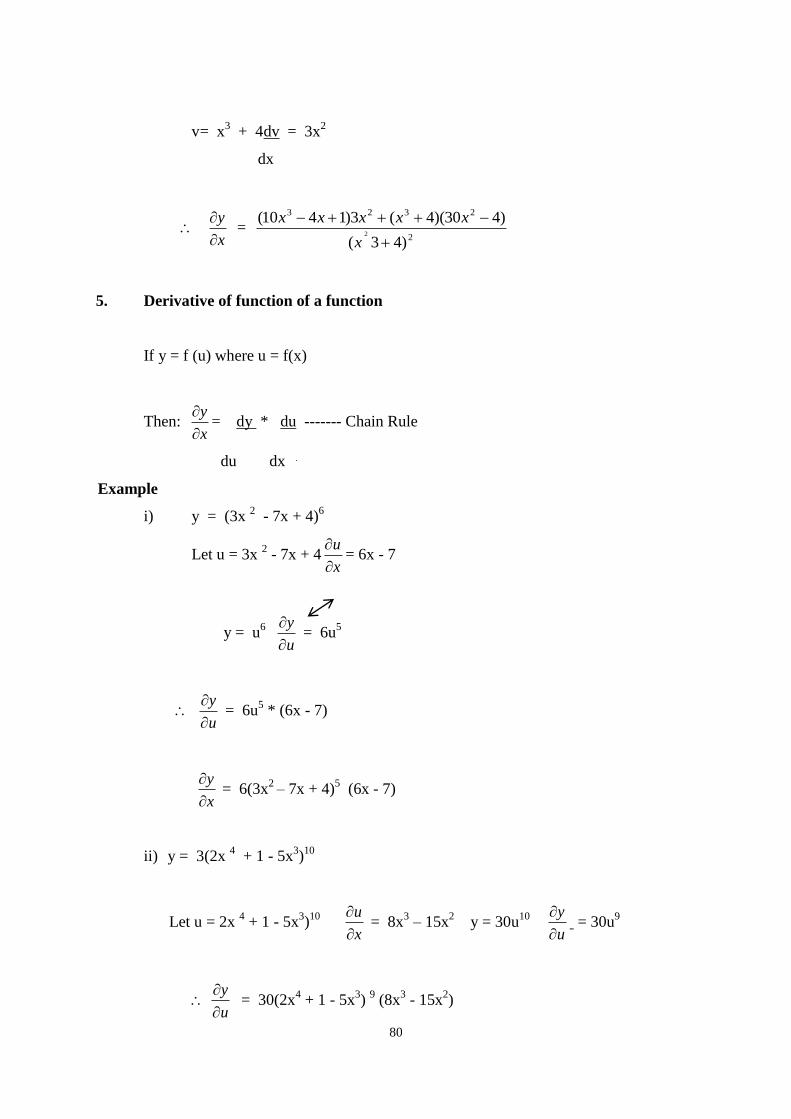
80

v = x3 + 4 dv = 3x

2

dx

x

y

=

2

2323

)43(

)430)(4(3)1410(2

x

xxxxx

5. Derivative of function of a function

If y = f (u) where u = f(x)

Then: x

y

= dy * du ------- Chain Rule

du dx

Example

i) y = (3x 2 - 7x + 4)

6

Let u = 3x 2 - 7x + 4

x

u

= 6x - 7

y = u6

u

y

= 6u

5

u

y

= 6u

5 * (6x - 7)

x

y

= 6(3x

2 – 7x + 4)

5 (6x - 7)

ii) y = 3(2x 4 + 1 - 5x

3)10

Let u = 2x 4 + 1 - 5x

3)10

x

u

= 8x

3 – 15x

2 y = 30u

10

u

y

= 30u

9

u

y

= 30(2x

4 + 1 - 5x

3)

9 (8x

3 - 15x

2)

81

u

y

= 30u (2x

4 + 1 – 5x

3)9

(8x3 - 15x

2)

Alternative method

Consider the function: y = (3x2 – 7x +4)

6 differentiated earlier. Let what is in the bracket be

big X.

Therefore, y =X6

which when differentiated yields x

y

= 6X

5

To obtain the eventual derivative, multiply this result by the derivative of the bracket as

follows;

x

y

= 6X

5 (6x -7)

But we know that X = 3x2 – 7x +4 so that:

x

y

= 6(3x

2 – 7x +4)

5 (6x -7)

Other examples

i) y = 3(2x 4 + 1 - 5x

3)10

3x10

= 30x9

x

y

= 30(2x

4 + 1 - 5x

3)

9 (8x

3 - 15x

2)

ii) y = 4 (17x5 + 12x

2 + x – 7)

3/2 4x

3/2 = 6x

1/2

x

y

= 6 (17x

5 + 12x

2 + x - 7)

1/2 (85x

4 + 24x + 1)

7.7 Higher order Derivatives

Sometimes its necessary to differentiate a function more than once and the results of

successive differentiations are known as higher order derivatives.

e.g. Consider a moving body e.g. a car.

Distance = f(time) ………. Initial (parent) function.

82

d (distance) = speed/velocity ------- 1st order derivative

d(time)

d(speed) = Acceleration -------------- 2nd

order derivative

d(time)

d = (Acceleration) = ?

d(time)

Activity 7.2

Determine the successive differentiation for the following functions

i) y = x2

x

y

= 2x

2x

y

=

3

2

x

y

= 2

x

y

3

= 0

ii) y = 3 - x4

+ 8x

x

y

= - 4x

3 + 8

2

2

x

y

= -12 x

2

3

3

x

y

= -24x

4

4

x

y

= -24

5

5

x

y

= 0

iii) x

y = y = 2x

-1

x

y

= -2x

-2

2

2

x

y

= 4 x

3

3

3

x

y

= -12x

-4

4

4

x

y

= 48x

-5

83

7.8

Summary

In this lecture, we have extended the ideas of differentiation to non-linear

functions. We have seen the concept of the limit and its importance in

differentiation. We also dealt with differentiation using the definition of the

derivate, that is, differentiation using first principles. We then looked at the

basic techniques or rules of differentiation which greatly simplify the

differentiation process. Finally, we looked at successive differentiation, also

known as higher order derivatives.

84

LECTURES EIGHT

APPLICATIONS OF DIFFERENTIATION

Lecture Outlines

8.1 Introduction

8.2 Objectives

8.3 Turning Points

8.4 Revenue, Cost and Profit Functions

8.5 Elasticity

8.6 Summary

8.1 Introduction

Welcome to Lecture Eight. In Lecture Seven, we learned the techniques of differentiation.

We are now ready to use these tools in solving business and economic problems.

Objectives

At the end of this lecture, you should be able to:

1. Identify stationary points.

2. Distinguish between a maximum and a minimum turning point.

3. Apply differentiation techniques to optimize business variables.

4. Determine price elasticity of demand.

8.3 Turning points

Optimisation, which is the process of either maximising or minimising some commercial

activity or quantity is at the core of most business problems e.g. maximise revenue, output,

productivity etc. Minimisation has to do with minimising costs, waste, loss etc.

The key to optimisation is to identify turning points (also known as critical or stationary

points) for the relevant functions.

8.2

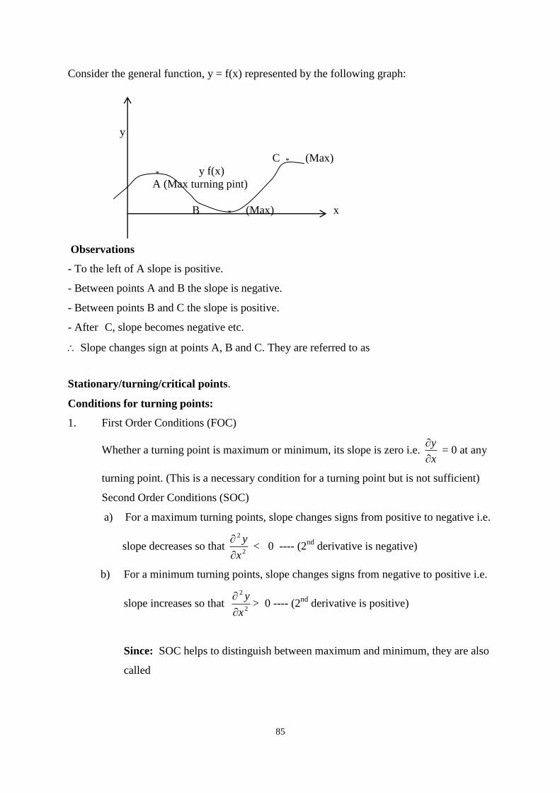
85

Consider the general function, y = f(x) represented by the following graph:

y

C * (Max)

* y f(x)

A (Max turning pint)

B * (Max) x

Observations

- To the left of A slope is positive.

- Between points A and B the slope is negative.

- Between points B and C the slope is positive.

- After C, slope becomes negative etc.

Slope changes sign at points A, B and C. They are referred to as

Stationary/turning/critical points.

Conditions for turning points:

1. First Order Conditions (FOC)

Whether a turning point is maximum or minimum, its slope is zero i.e. x

y

= 0 at any

turning point. (This is a necessary condition for a turning point but is not sufficient)

Second Order Conditions (SOC)

a) For a maximum turning points, slope changes signs from positive to negative i.e.

slope decreases so that 2

2

x

y

< 0 ---- (2

nd derivative is negative)

b) For a minimum turning points, slope changes signs from negative to positive i.e.

slope increases so that 2

2

x

y

> 0 ---- (2

nd derivative is positive)

Since: SOC helps to distinguish between maximum and minimum, they are also

called

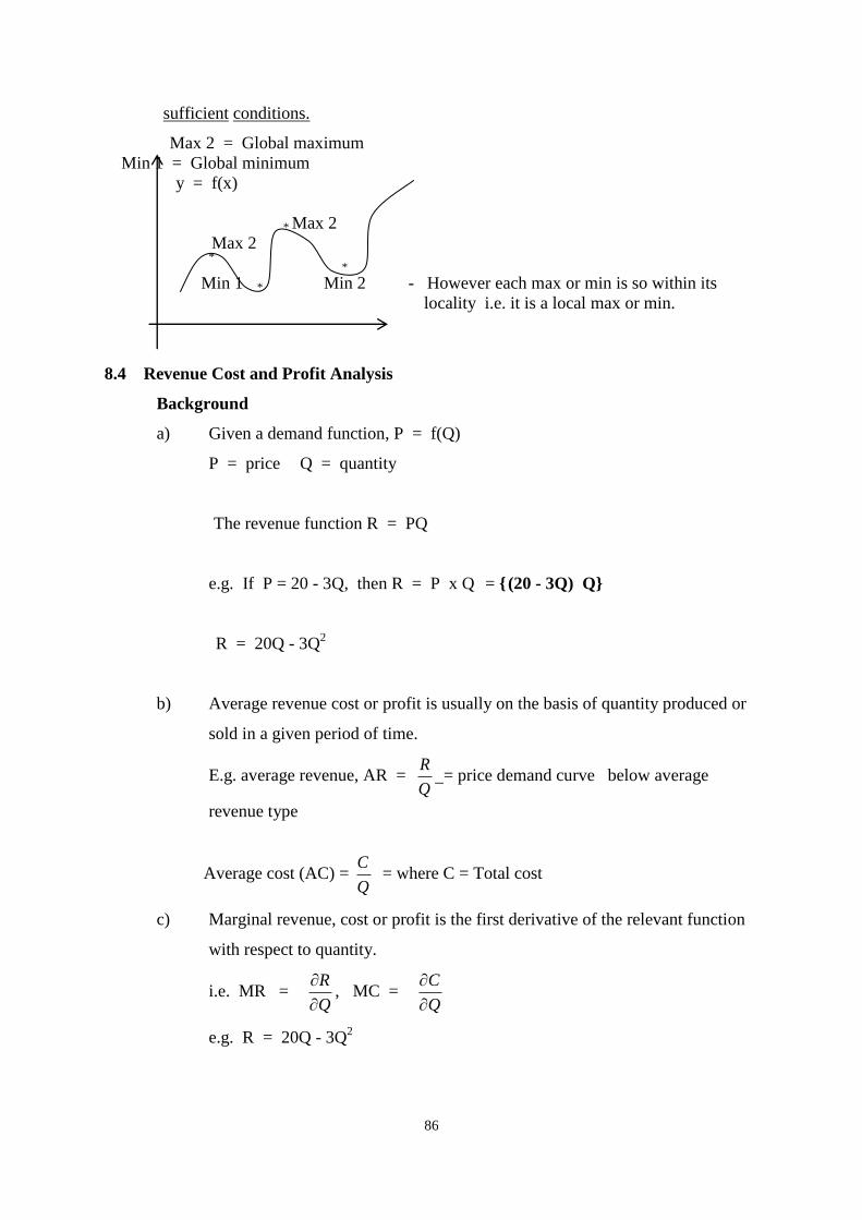
86

sufficient conditions.

Max 2 = Global maximum

Min 1 = Global minimum

y = f(x)

* Max 2

Max 2

*

*

Min 1

* Min 2 - However each max or min is so within its

locality i.e. it is a local max or min.

8.4 Revenue Cost and Profit Analysis

Background

a) Given a demand function, P = f(Q)

P = price Q = quantity

The revenue function R = PQ

e.g. If P = 20 - 3Q, then R = P x Q = { (20 - 3Q) Q}

R = 20Q - 3Q2

b) Average revenue cost or profit is usually on the basis of quantity produced or

sold in a given period of time.

E.g. average revenue, AR = Q

R = price demand curve below average

revenue type

Average cost (AC) = Q

C = where C = Total cost

c) Marginal revenue, cost or profit is the first derivative of the relevant function

with respect to quantity.

i.e. MR = Q

R

, MC =

Q

C

e.g. R = 20Q - 3Q2

87

MR = Q

R

= 20 - 6Q AR (price) =

Q

R = 20 - 3Q

Exercises

A firm’s demand function is given as P = 24 – 3x

Where P = price and x quantity produced and sold.

Determine the output for maximum revenue and show it is a maximum. What is the price at

maximum revenue.

Solution:

P = 24 - 3x

P = PX = (24 – 3x)x R = 24x - 3x2

FOC: For maximum or minimum X

R

= 0

X

R

= 24 - 6x = 0 X =

6

24 = 4 units

SOC: 2

2

x

R

= -6 < 0 Max

Maximum revenue, R maximum = 24(4) - 3(4)2 = Sh.48

Hence price when revenue is maximum = P = 24 - 3(4) = Sh.12

Problem

The revenue function of a product is R = 28q - q2 and the unit variable cost v = q – 8 while

fixed cost is Sh.64.

Determine the following:

a) Total cost function

b) Profit function

c) Output and price for maximum profit.

d) Show that the output for maximum profit is not necessarily the same as the output for

maximum revenue.

e) Represent the above functions on a graphical sketch.

Solution:

a) Total cost C = Total variable cost + Fixed cost

88

C = (q - 8)q + 64 = 64 + q2 – 8q

C = q2 - 8q + 64

b) Profit function, = R - C

= 28q - q2 - (q

2 - 8q + 64)

= 36q - 2q2

- 64

b) Output and price for maximum profit:

FOC: For maximum or minimum q

= 36 - 4q = 0

q = 4

36 = 9 units

SOC: 2

2

q

= -4 < Maximum turning point

Maximum profit, maximum = 36(9) - 2(9)2 - 64 = Sh.98

Price to be charged to obtain maximum profits ( maximum)

Q

P =

q

R = 28q - q

2 = 28 - q

When q = 9 units, P = 28 - 9 = Sh.19

d) Output which maximizes profit, q = 9 units.

Output for maximum revenue.

R = 28q - q2

FOC For maximum or minimum q

R

= 28 - 2q = 0

q = 2

28 = 14 units

SOC: 2

2

q

R

= - 2 < 0 = Maximum

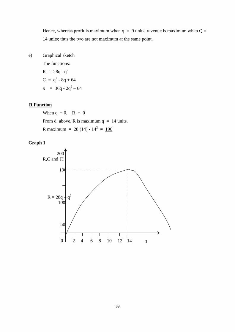
89

Hence, whereas profit is maximum when q = 9 units, revenue is maximum when Q =

14 units; thus the two are not maximum at the same point.

e) Graphical sketch

The functions:

R = 28q - q2

C = q2 - 8q + 64

= 36q - 2q2 – 64

R Function

When q = 0, R = 0

From d above, R is maximum q = 14 units.

R maximum = 28 (14) - 142 = 196

Graph 1

200

R,C and

196

R = 28q – q2

100

50

0 2 4 6 8 10 12 14 q

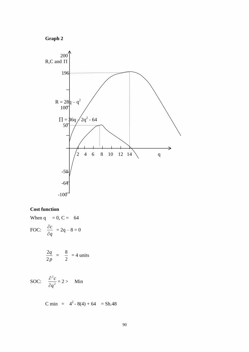
90

Graph 2

200

R,C and

196

R = 28q – q2

100

= 36q – 2q2 - 64

50

2 4 6 8 10 12 14 q

-50

-64

-100

Cost function

When q = 0, C = 64

FOC: q

c

= 2q – 8 = 0

p

q

2

2 =

2

8 = 4 units

SOC: 2

2

q

c

= 2 > Min

C min = 42

- 8(4) + 64 = Sh.48

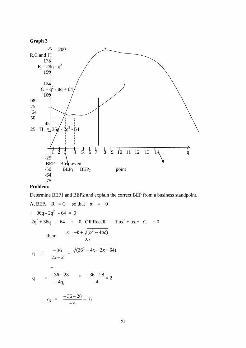
91

Graph 3

200 *

R,C and

175

R = 28q - q2

150

125

C = q2 - 8q + 64

100

98

75

64

50

45

25 = 36q - 2q2 - 64

1 2 3 4 5 6 7 8 9 10 11 12 13 14 q

-25

BEP = Breakeven

-50 BEP1 BEP2 point

-64

-75

Problem:

Determine BEP1 and BEP2 and explain the correct BEP from a business standpoint.

At BEP, R = C so that = 0

36q - 2q2

- 64 = 0

-2q2 + 36q - 64 = 0 OR Recall: If ax

2 + bx + C = 0

then: a

acbbx

2

)4( 2

q = 22

36

x +

)642436( 2 xx

q =

14

2836

q

= 2

4

2836

q2 = 164

2836

92

The correct break even point is = 2 units because thereafter the firm begins to make profit.

8.5 Elasticity

8.6

Summary

This lecture has dealt with applications of differentiation. The

concept of turning point and its importance in optimization was

explained.

We have also discussed the application of differentiation to revenue,

cost and profit analysis and the calculation of elasticity. In the next

lecture, we extend these ideas on differentiation to multivariate

functions.

Activity

a) Explain and graphically illustrate what is meant by he breakeven

point in business.

b) The average total cost of producing a commodity is given by

ATC = 1000/q + 100 – 5q + q2

where p is the price in shillings and q is

the quantity in kilogrammes. The expected sales of commodity are 390

units at the selling price of Sh. 10 and the sales would fall to 380 units if

the price is doubled to Sh.20

Required:

i) By using an example, explain what 1000/q in the

ATC equation represents economically.

ii) Determine the linear demand function in the form p =

a + bq where p = price and q = quantity.

iii) Determine the revenue function.

iv) Determine the profit function, output and price for

maximum profit and the maximum profit. Show that

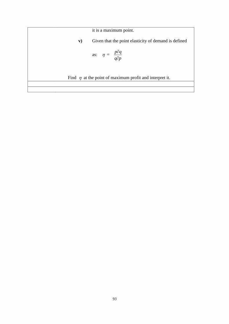
93

it is a maximum point.

v) Given that the point elasticity of demand is defined

as: = pq

qp

Find at the point of maximum profit and interpret it.

94

LECTURE NINE

FURTHER DIFFERENTIATION: MULTIVARIATE FUNCTIONS

Lecture Outlines

9.1 Introduction

9.2 Objectives

9.3 Partial Differentiation

9.4 Classical Optimisation: Presence of an Equality Constraint

9.5 The Total Differential

9.6 Summary

9.1 Introduction

Welcome to this lecture. In Lecture eight, we learned the application of differentiation to

functions of a single independent variable. For many business problems, dependent variables

are determined by two or more independent variables. This Lecture is concerned with

differentiation of such functions and their applications.

9.2

Objectives

At the end of this lecture, you should be able to:

1. Determine first order partial derivatives.

2. Determine second order partial derivatives.

3. Apply partial derivatives in optimizing business variables.

9.3 Partial Differentiation

So far, we have done differentiation of functions of one independent variable e.g.

i) Price = f (output)

ii) Revenue = f (output)

However there are many situations where the dependent variable is determined by two or

more independent variables e.g.

Sales = f (price, advertising budget, output etc)

Problem:

Optimisation of the dependent variable when we have two or more independent variables.

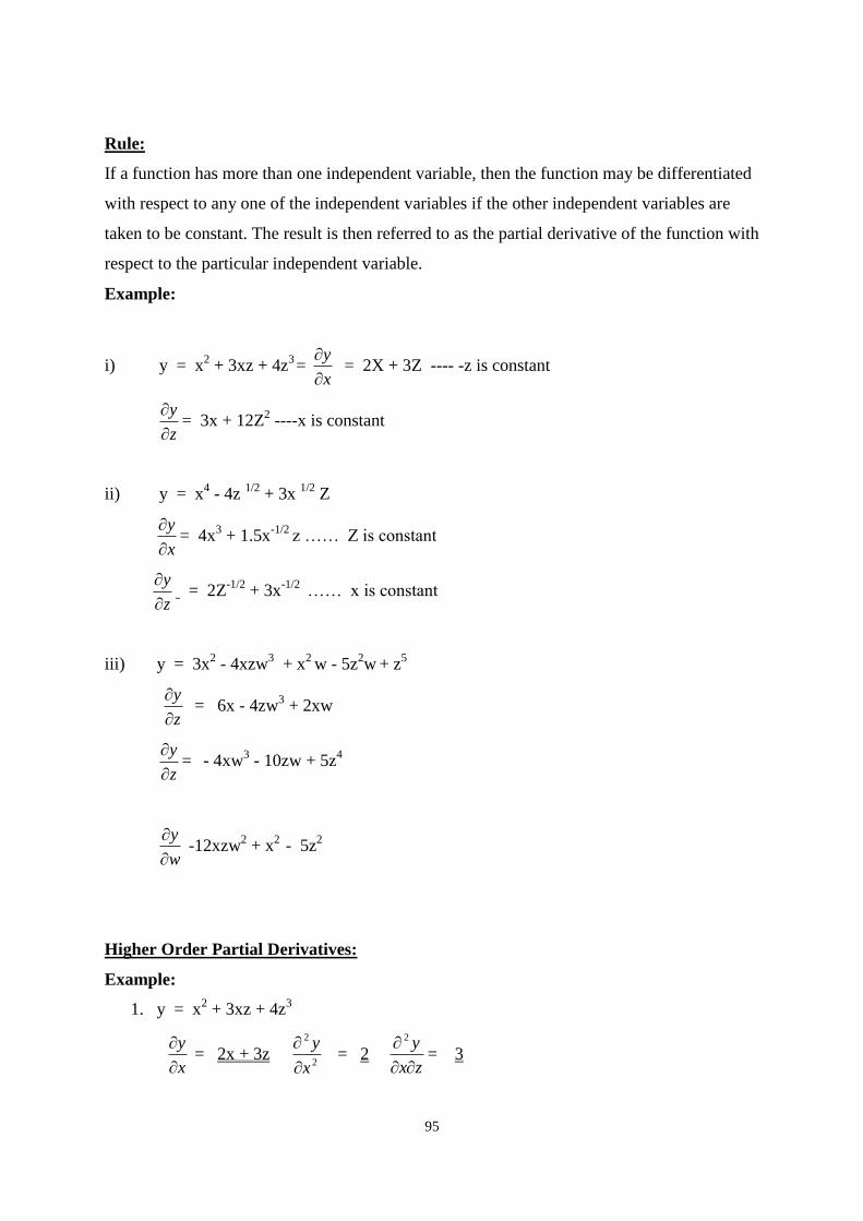
95

Rule:

If a function has more than one independent variable, then the function may be differentiated

with respect to any one of the independent variables if the other independent variables are

taken to be constant. The result is then referred to as the partial derivative of the function with

respect to the particular independent variable.

Example:

i) y = x2 + 3xz + 4z

3 =

x

y

= 2X + 3Z ---- -z is constant

z

y

= 3x + 12Z

2 ----x is constant

ii) y = x4 - 4z

1/2 + 3x

1/2 Z

x

y

= 4x

3 + 1.5x

-1/2 z …… Z is constant

z

y

= 2Z

-1/2 + 3x

-1/2 …… x is constant

iii) y = 3x2 - 4xzw

3 + x

2 w - 5z

2w

+ z

5

z

y

= 6x - 4zw

3 + 2xw

z

y

=

- 4xw

3 - 10zw + 5z

4

w

y

-12xzw

2 + x

2 - 5z

2

Higher Order Partial Derivatives:

Example:

1. y = x2 + 3xz + 4z

3

x

y

= 2x + 3z

2

2

x

y

= 2

zx

y

2

= 3

96

x

y

= 3x + 12Z

2

2

2

z

y

= 24z

xz

y

2

= 3

Note:

tz

y

2

xz

y

2

------------- Young's theorem

2. y = 3xw - w3 + 2x

2 w

iii) x

y

= 3x + 4xw

iv) w

y

= 3x - 3w

2 + 2x

2

iii) Show that wx

y

2

= xw

y

2

x

wx

y43

2

Equal

xxw

y43

2

Maxima and Minima for Two Independent Variables

Consider the function

Y = f (xz)

To obtain the critical/stationary points.

FOC: = x

y

z

y

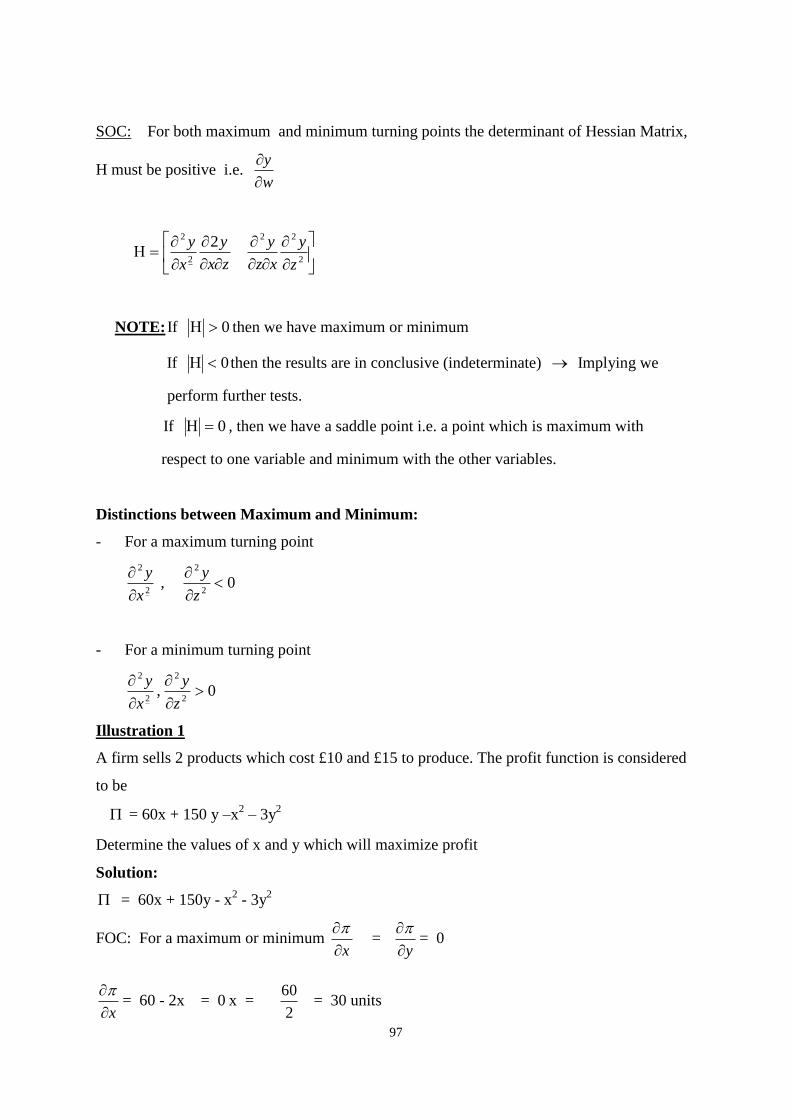
97

SOC: For both maximum and minimum turning points the determinant of Hessian Matrix,

H must be positive i.e. w

y

zx

y

x

y

22

2

2

22

z

y

xz

y

NOTE: If 0 then we have maximum or minimum

If 0 then the results are in conclusive (indeterminate) Implying we

perform further tests.

If 0 , then we have a saddle point i.e. a point which is maximum with

respect to one variable and minimum with the other variables.

Distinctions between Maximum and Minimum:

- For a maximum turning point

2

2

x

y

, 0

2

2

z

y

- For a minimum turning point

2

2

x

y

, 0

2

2

z

y

Illustration 1

A firm sells 2 products which cost £10 and £15 to produce. The profit function is considered

to be

= 60x + 150 y –x2 – 3y

2

Determine the values of x and y which will maximize profit

Solution:

= 60x + 150y - x2 - 3y

2

FOC: For a maximum or minimum x

=

y

= 0

x

= 60 - 2x = 0 x =

2

60 = 30 units

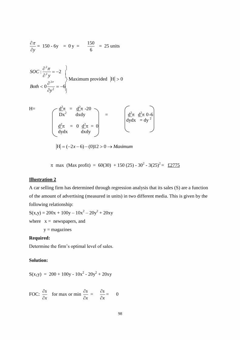
98

y

= 150 - 6y = 0 y =

6

150 = 25 units

60

2:

2

2

2

2

yBoth

ySOC

Maximum provided 0

H= d2 = d

2 -2 0

Dx2 dxdy = d

2 d

2 0 -6

dydx = dy

2

d2 = 0 d

2 = 0

dydx dxdy

Maximumx 012)0()62(

max (Max profit) = 60(30) + 150 (25) - 302 - 3(25)

2 = £2775

Illustration 2

A car selling firm has determined through regression analysis that its sales (S) are a function

of the amount of advertising (measured in units) in two different media. This is given by the

following relationship:

S(x,y) = 200x + 100y – 10x2 – 20y

2 + 20xy

where x = newspapers, and

y = magazines

Required:

Determine the firm’s optimal level of sales.

Solution:

S(x1y) = 200 + 100y - 10x2 - 20y

2 + 20xy

FOC: x

s

for max or min

x

s

=

x

s

= 0

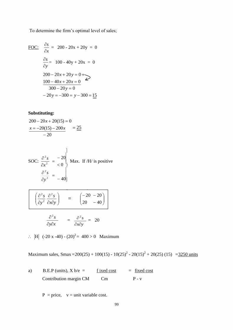
99

To determine the firm’s optimal level of sales;

FOC: x

s

= 200 - 20x + 20y = 0

y

s

= 100 - 40y + 20x = 0

1530030020

020300

02040100

02020200

yy

y

xx

yx

Substituting:

20

200)15(20

0)15(2020200

xx

x

25

SOC:

2

2

2

2

y

s

x

s

40

0

20 Max. If /H/ is positive

H =

20

20

40

20

xy

s

2

= yx

s

2

= 20

(-20 x -40) - (20)2 = 400 > 0 Maximum

Maximum sales, Smax = 200(25) + 100(15) - 10(25)2 - 20(15)

2 + 20(25) (15) = 3250 units

a) B.E.P (units), X b/e = f ixed cost = fixed cost

Contribution margin CM Cm P - v

P = price, v = unit variable cost.

2

2

y

s

yx

s2

=

20

20

40

20

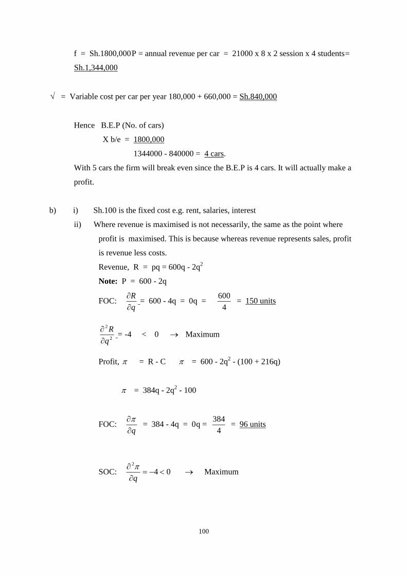
100

f = Sh.1800,000 P = annual revenue per car = 21000 x 8 x 2 session x 4 students =

Sh.1,344,000

= Variable cost per car per year 180,000 + 660,000 = Sh.840,000

Hence B.E.P (No. of cars)

X b/e = 1800,000

1344000 - 840000 = 4 cars.

With 5 cars the firm will break even since the B.E.P is 4 cars. It will actually make a

profit.

b) i) Sh.100 is the fixed cost e.g. rent, salaries, interest

ii) Where revenue is maximised is not necessarily, the same as the point where

profit is maximised. This is because whereas revenue represents sales, profit

is revenue less costs.

Revenue, R = pq = 600q - 2q2

Note: P = 600 - 2q

FOC: q

R

= 600 - 4q = 0 q =

4

600 = 150 units

2

2

q

R

= -4 < 0 Maximum

Profit, = R - C = 600 - 2q2 - (100 + 216q)

= 384q - 2q2 - 100

FOC: q

= 384 - 4q = 0 q =

4

384 = 96 units

SOC: 042

q

Maximum

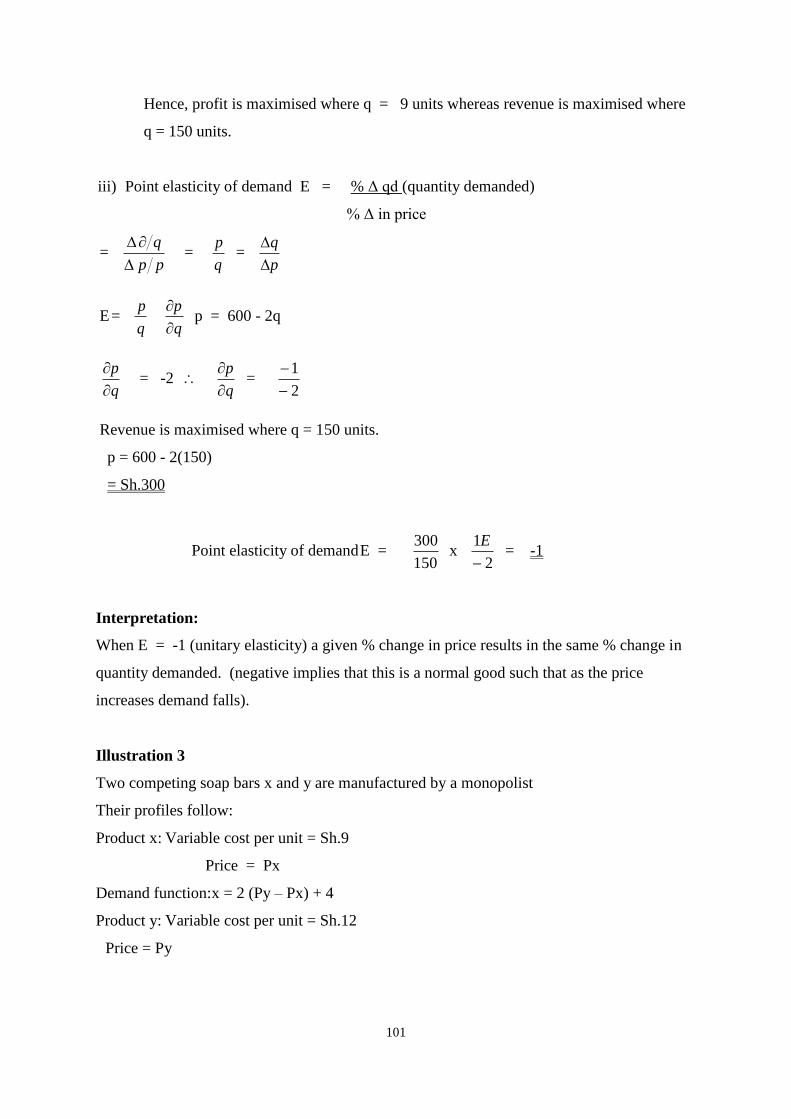
101

Hence, profit is maximised where q = 9 units whereas revenue is maximised where

q = 150 units.

iii) Point elasticity of demand E = % Δ qd (quantity demanded)

% Δ in price

= pp

q

=

q

p =

p

q

E = q

p

q

p

p = 600 - 2q

q

p

= -2

q

p

=

2

1

Revenue is maximised where q = 150 units.

p = 600 - 2(150)

= Sh.300

Point elasticity of demand E = 150

300 x

2

1

E = -1

Interpretation:

When E = -1 (unitary elasticity) a given % change in price results in the same % change in

quantity demanded. (negative implies that this is a normal good such that as the price

increases demand falls).

Illustration 3

Two competing soap bars x and y are manufactured by a monopolist

Their profiles follow:

Product x: Variable cost per unit = Sh.9

Price = Px

Demand function:x = 2 (Py – Px) + 4

Product y: Variable cost per unit = Sh.12

Price = Py

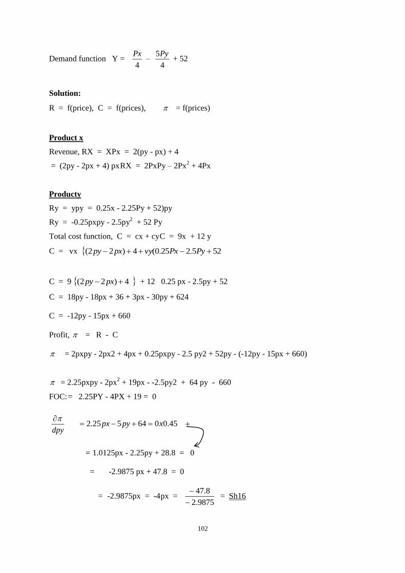
102

Demand function Y = 4

Px –

4

5Py + 52

Solution:

R = f(price), C = f(prices), = f(prices)

Product x

Revenue, RX = XPx = 2(py - px) + 4

= (2py - 2px + 4) px RX = 2PxPy – 2Px2 + 4Px

Producty

Ry = ypy = 0.25x - 2.25Py + 52)py

Ry = -0.25pxpy - 2.5py2 + 52 Py

Total cost function, C = cx + cy C = 9x + 12 y

C = vx 525.225.0(4)22( PyPxvypxpy

C = 9 4)22( pxpy + 12 0.25 px - 2.5py + 52

C = 18py - 18px + 36 + 3px - 30py + 624

C = -12py - 15px + 660

Profit, = R - C

= 2pxpy - 2px2 + 4px + 0.25pxpy - 2.5 py2 + 52py - (-12py - 15px + 660)

= 2.25pxpy - 2px2 + 19px - -2.5py2 + 64 py - 660

FOC: = 2.25PY - 4PX + 19 = 0

dpy

45.0064525.2 xpypx

= 1.0125px - 2.25py + 28.8 = 0

= -2.9875 px + 47.8 = 0

= -2.9875px = -4 px = 9875.2

8.47

= Sh16

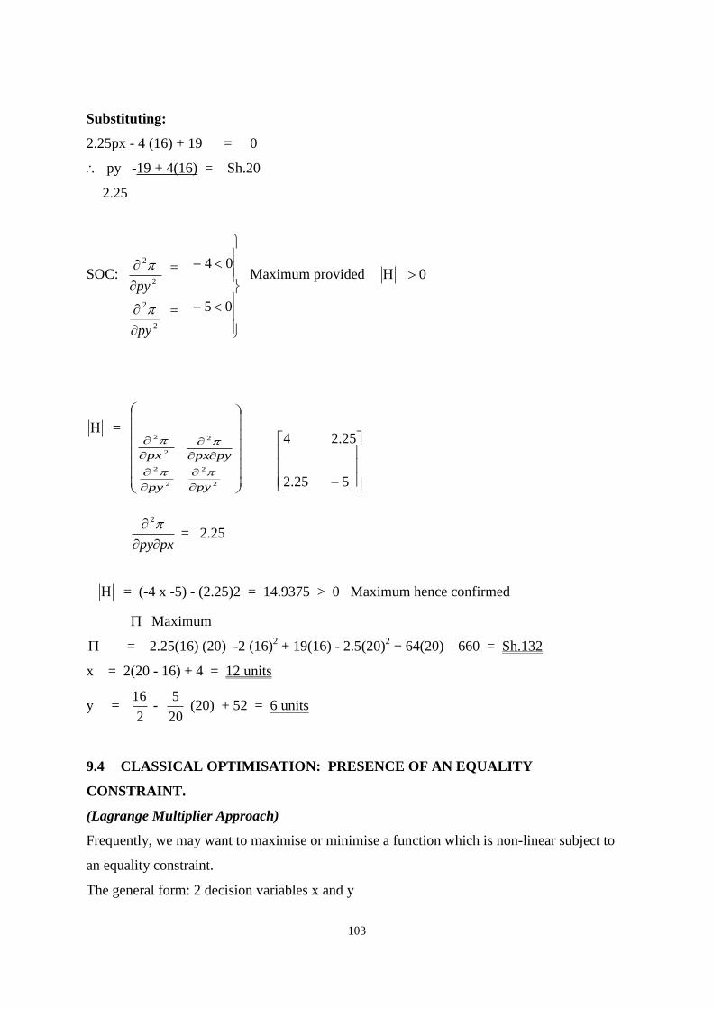
103

Substituting:

2.25px - 4 (16) + 19 = 0

py -19 + 4(16) = Sh.20

2.25

SOC:

2

2

2

2

py

py

05

04 Maximum provided 0

=

2

2

2

2

py

px

2

2

2

py

pypx

25.2

4

5

25.2

pxpy

2

= 2.25

= (-4 x -5) - (2.25)2 = 14.9375 > 0 Maximum hence confirmed

Maximum

= 2.25(16) (20) -2 (16)2 + 19(16) - 2.5(20)

2 + 64(20) – 660 = Sh.132

x = 2(20 - 16) + 4 = 12 units

y = 2

16 -

20

5 (20) + 52 = 6 units

9.4 CLASSICAL OPTIMISATION: PRESENCE OF AN EQUALITY

CONSTRAINT.

(Lagrange Multiplier Approach)

Frequently, we may want to maximise or minimise a function which is non-linear subject to

an equality constraint.

The general form: 2 decision variables x and y

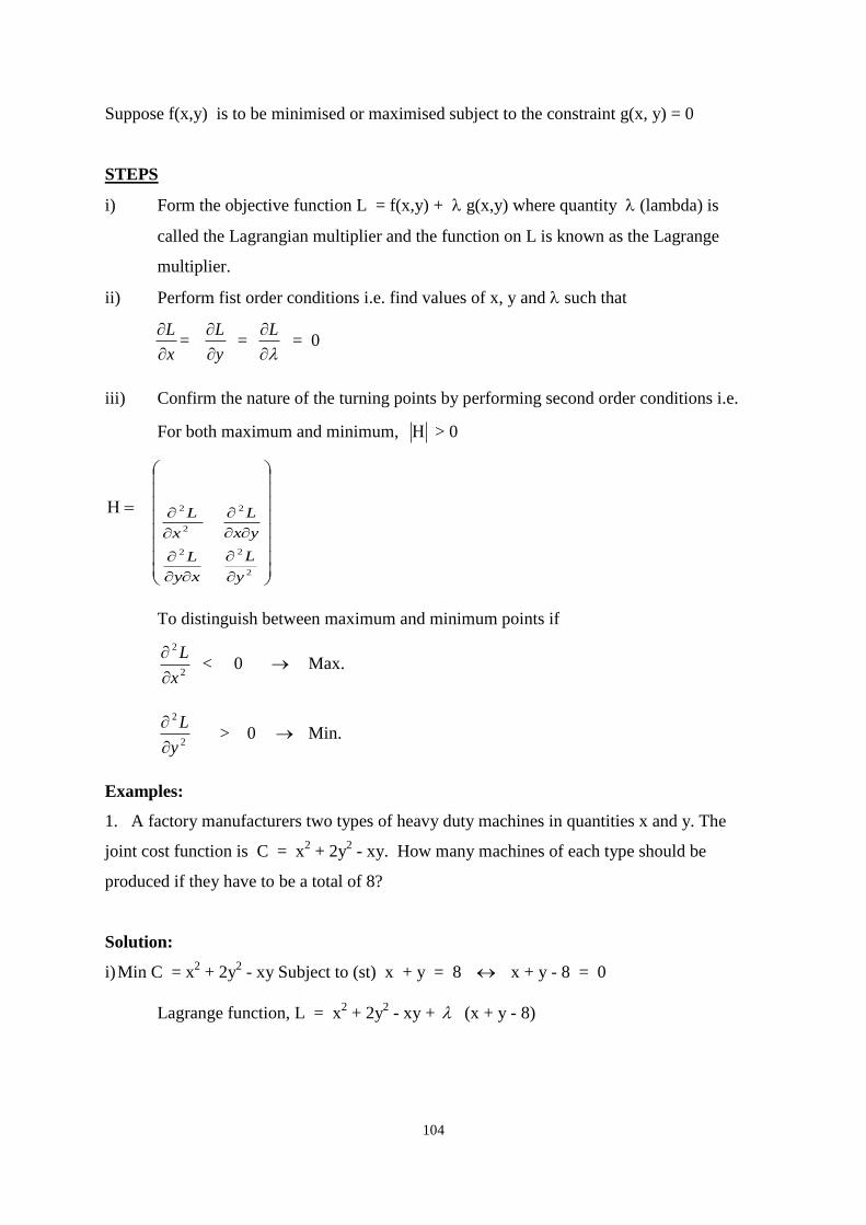
104

Suppose f(x,y) is to be minimised or maximised subject to the constraint g(x, y) = 0

STEPS

i) Form the objective function L = f(x,y) + g(x,y) where quantity (lambda) is

called the Lagrangian multiplier and the function on L is known as the Lagrange

multiplier.

ii) Perform fist order conditions i.e. find values of x, y and such that

x

L

=

y

L

=

L = 0

iii) Confirm the nature of the turning points by performing second order conditions i.e.

For both maximum and minimum, > 0

xy

L

x

L

2

2

2

2

2

2

y

L

yx

L

To distinguish between maximum and minimum points if

2

2

x

L

< 0 Max.

2

2

y

L

> 0 Min.

Examples:

1. A factory manufacturers two types of heavy duty machines in quantities x and y. The

joint cost function is C = x2 + 2y

2 - xy. How many machines of each type should be

produced if they have to be a total of 8?

Solution:

i) Min C = x2 + 2y

2 - xy Subject to (st) x + y = 8 x + y - 8 = 0

Lagrange function, L = x2 + 2y

2 - xy + (x + y - 8)

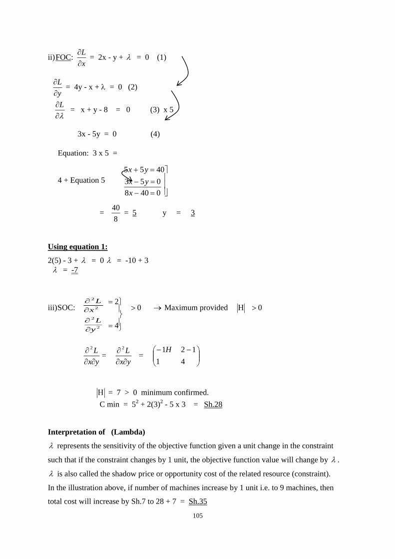
105

ii) FOC: x

L

= 2x - y + = 0 (1)

y

L

= 4y - x + = 0 (2)

L = x + y - 8 = 0 (3) x 5

3x - 5y = 0 (4)

Equation: 3 x 5 =

4 + Equation 5

0408

053

4055

x

yx

yx

= 8

40 = 5 y = 3

Using equation 1:

2(5) - 3 + = 0 = -10 + 3

= -7

iii) SOC:

2

2

2

2

y

L

x

L

4

2 0 Maximum provided 0

yx

L

2

= yx

L

2

=

1

1H

4

12

= 7 > 0 minimum confirmed.

C min = 52 + 2(3)

2 - 5 x 3 = Sh.28

Interpretation of (Lambda)

represents the sensitivity of the objective function given a unit change in the constraint

such that if the constraint changes by 1 unit, the objective function value will change by .

is also called the shadow price or opportunity cost of the related resource (constraint).

In the illustration above, if number of machines increase by 1 unit i.e. to 9 machines, then

total cost will increase by Sh.7 to 28 + 7 = Sh.35

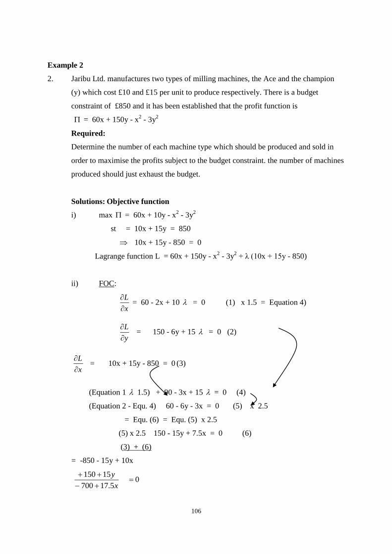
106

Example 2

2. Jaribu Ltd. manufactures two types of milling machines, the Ace and the champion

(y) which cost £10 and £15 per unit to produce respectively. There is a budget

constraint of £850 and it has been established that the profit function is

= 60x + 150y - x2 - 3y

2

Required:

Determine the number of each machine type which should be produced and sold in

order to maximise the profits subject to the budget constraint. the number of machines

produced should just exhaust the budget.

Solutions: Objective function

i) max = 60x + 10y - x2 - 3y

2

st = 10x + 15y = 850

10x + 15y - 850 = 0

Lagrange function L = 60x + 150y - x2 - 3y

2 + λ (10x + 15y - 850)

ii) FOC:

x

L

= 60 - 2x + 10 = 0 (1) x 1.5 = Equation 4)

y

L

= 150 - 6y + 15 = 0 (2)

x

L

= 10x + 15y - 850 = 0 (3)

(Equation 1 1.5) + 90 - 3x + 15 = 0 (4)

(Equation 2 - Equ. 4) 60 - 6y - 3x = 0 (5) x 2.5

= Equ. (6) = Equ. (5) x 2.5

(5) x 2.5 150 - 15y + 7.5x = 0 (6)

(3) + (6)

= -850 - 15y + 10x

x

y

5.17700

15150

0

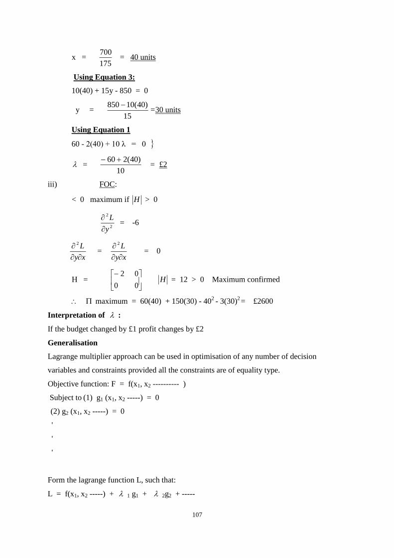
107

x = 175

700 = 40 units

Using Equation 3:

10(40) + 15y - 850 = 0

y = 15

)40(10850 = 30 units

Using Equation 1

60 - 2(40) + 10 λ = 0

= 10

)40(260 = £2

iii) FOC:

< 0 maximum if H > 0

2

2

y

L

= -6

xy

L

2

= xy

L

2

= 0

=

0

2

0

0 H = 12 > 0 Maximum confirmed

maximum = 60(40) + 150(30) - 402

- 3(30)2 = £2600

Interpretation of :

If the budget changed by £1 profit changes by £2

Generalisation

Lagrange multiplier approach can be used in optimisation of any number of decision

variables and constraints provided all the constraints are of equality type.

Objective function: F = f(x1, x2 ---------- )

Subject to (1) g1 (x1, x2 -----) = 0

(2) g2 (x1, x2 -----) = 0

'

'

'

Form the lagrange function L, such that:

L = f(x1, x2 -----) + 1 g1 + 2g2 + -----

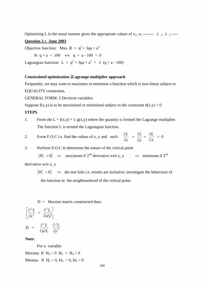
108

Optimizing L in the usual manner gives the appropriate values of x1, x2 -------- 1, 2 -----

Question 2 c June 2003

Objective function: Max. R = q2

+ 3qa + a2

St q + a = 100 q + a - 100 = 0

Lagrangian function: L = q2 + 3qa + a

2 + (q + a - 100)

Constrained optimisation {Lagrange multiplier approach

Frequently, we may want to maximise or minimise a function which is non-linear subject to

EQUALITY constraints.

GENERAL FORM: 2 Decision variables:

Suppose f(x,y) is to be maximised or minimised subject to the constraint d(x,y) = 0

STEPS

1. Form the L = f(x,y) + g(x,y) where the quantity is formed the Lagrange multiplier.

The function L is termed the Lagrangian function

2. Form F.O.C i.e. find the values of x, y and such x

L

=

y

L

=

L = 0

3. Perform S.O.C to determine the nature of the critical point

H 0 maximum if 2nd

derivative writ x, y minimum if 2nd

derivative writ x, y

H 0 the test fails i.e. results are inclusive; investigate the behaviour of

the function in the neighbourhood of the critical point.

= Hessian matrix constructed thus:

2

2

x

L =

yx

L2

= Ly

L

2

2

2

y

L

Note:

For n variable:

Maxima If H2 > 0 H3 < H4 > 0

Minima If H2 < 0, H3 < 0, H4 < 0

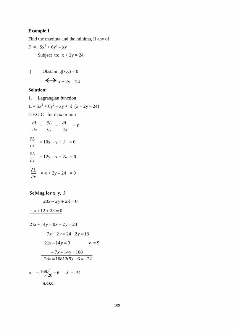
109

Example 1

Find the maxima and the minima, if any of

F = Sx2 + 6y

2 – xy

Subject to: x + 2y = 24

i) Obstain g(x,y) = 0

x + 2y = 24

Solution:

1. Lagrangian function

L = 5x2 + 6y

2 – xy + (x + 2y – 24)

2. F.O.C for max or min

x

L

=

y

L

=

x

L

= 0

x

L

= 10x – y + = 0

y

L

= 12y – x = 2 = 0

x

L

= x + 2y – 24 = 0

Solving for x, y,

02220 yx

24201421

0212

yxyx

x

2427 yx 182 y

01421 yx y = 9

26)9(1681228

168147

x

yx

x = 28

168 = 6 = -51

S.O.C

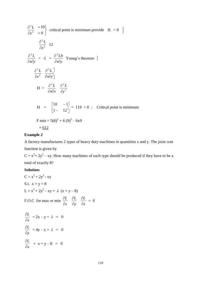
110

2

2

x

L

0

10 critical point is minimum provide > 0

2

2

x

L

12

yx

L

2

= -1 = yx

Lb

2

Young’s theorem

2

2

x

L

yx

L2

= xx

L

2

2

2

y

L

=

1

10

12

1 = 119 > 0 Critical point is minimum

F min = 5(6)2 + 6 (9)

2 – 6x9

= 612

Example 2

A factory manufactures 2 types of heavy duty machines in quantities x and y. The joint cost

function is given by

C = x2+ 2y

2 – xy. How many machines of each type should be produced if they have to be a

total of exactly 8?

Solution:

C = x2

+ 2y2

- xy

S.t. x + y = 8

L = x2

+ 2y2

– xy + (x + y – 8)

F.O.C for max or min x

L

y

L

x

L

= 0

x

L

= 2x – y + = 0

y

L

= 4y – x + = 0

x

L

= x + y – 8 = 0

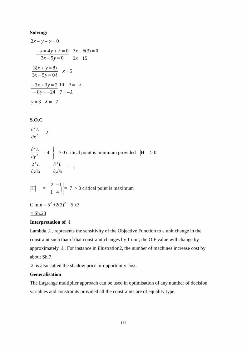
111

Solving:

02 yx

053

04

yx

yx

153

0)3(53

x

x

053

)8(3

yx

yx 5x

248

233

y

yx

7

310

3y 7

S.O.C

2

2

x

L

= 2

2

2

y

L

= 4

> 0 critical point is minimum provided > 0

xy

L

22 =

xy

L

2

= -1

=

1

2

4

1= 7 > 0 critical point is maximum

C min = 52 +2(3)

2 – 5 x3

= Sh.28

Interpretation of

Lambda, , represents the sensitivity of the Objective Function to a unit change in the

constraint such that if that constraint changes by 1 unit, the O.F value will change by

approximately . For instance in illustration2, the number of machines increase cost by

about Sh.7.

is also called the shadow price or opportunity cost.

Generalisation

The Lagrange multiplier approach can be used in optimisation of any number of decision

variables and constraints provided all the constraints are of equality type.

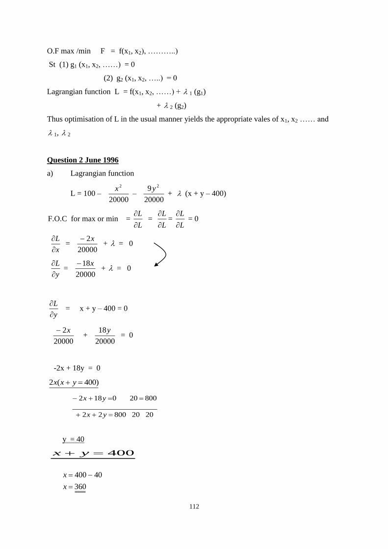
112

O.F max /min F = f(x1, x2), ………..)

St (1) g1 (x1, x2, ……) = 0

(2) g2 (x1, x2, …..) = 0

Lagrangian function L = f(x1, x2, ……) + 1 (g1)

+ 2 (g2)

Thus optimisation of L in the usual manner yields the appropriate vales of x1, x2 …… and

1, 2

Question 2 June 1996

a) Lagrangian function

L = 100 – 20000

2x –

20000

9 2y + (x + y – 400)

F.O.C for max or min = L

L

=

L

L

=

L

L

= 0

x

L

=

20000

2x + = 0

y

L

=

20000

18x + = 0

y

L

= x + y – 400 = 0

20000

2x +

20000

18y = 0

-2x + 18y = 0

)400(2 yxx

202080022

800200182

yx

yx

y = 40

400 yx

360

40400

x

x

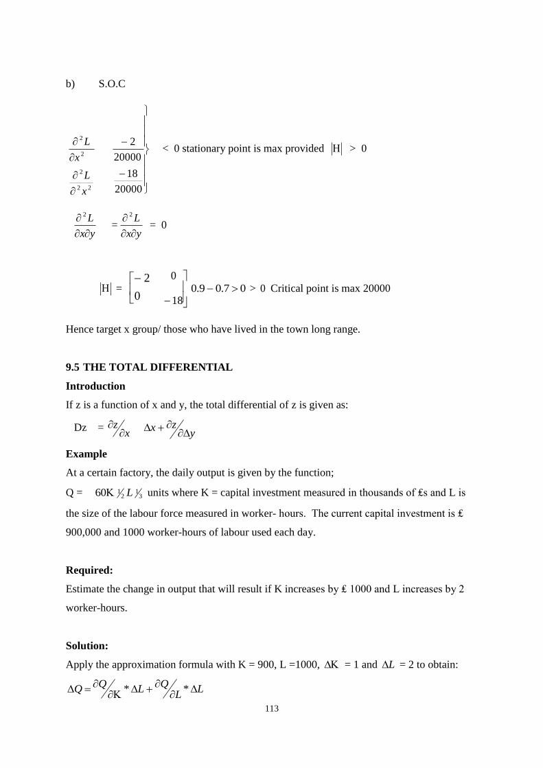
113

b) S.O.C

22

2

2

2

x

L

x

L

20000

18

20000

2 < 0 stationary point is max provided > 0

yx

L

2

= yx

L

2

= 0

=

0

2

18

007.09.0 > 0 Critical point is max 20000

Hence target x group/ those who have lived in the town long range.

9.5 THE TOTAL DIFFERENTIAL

Introduction

If z is a function of x and y, the total differential of z is given as:

Dz = x

z

y

zx

Example

At a certain factory, the daily output is given by the function;

Q = 31

2160 L units where K = capital investment measured in thousands of ₤s and L is

the size of the labour force measured in worker- hours. The current capital investment is ₤

900,000 and 1000 worker-hours of labour used each day.

Required:

Estimate the change in output that will result if K increases by ₤ 1000 and L increases by 2

worker-hours.

Solution:

Apply the approximation formula with K = 900, L =1000, = 1 and L = 2 to obtain:

LL

QL

QQ

**

114

LLKKLKQ **20*30 32

21

31

31

2*)1000()900(201*)1000()900(30(30 32

21

31

21 Q

2*)100

1)(30(201*)10)(30

1(30 Q

22Q units

Hence, output is expected to increase by approximately 122 units..

9.6

Summary

In this lecture, we have studied how to perform differentiation when we have

two or more predictor variables. We dealt with the case when a single

predictor is varying while the others are constant and applications. We also

looked at the case when all predictors are varying at the same time and their

business applications. Finally, we looked at optimisation in the case where

there is a single constraint of equality type.

115

Activity

The return on two types of investments is given by the following function:

R = - 0.00008x12

- 0.00012x2 2

+0.00016 x1 x2 + 0.4 x1 + 0.8 x2

Where x1 and x2 are the sums allocated to investment 1 and 2 respectively.

Required:

a) Determine the amounts to allocate to investments 1 and 2 in order to

maximize return on investment if the amount of money available to

invest is unlimited.

b) What amount would be allocated to investments 1 and 2 if the

investible money available is limited to $ 10,000 and all of it is

unlimited?

c) What is the difference in return on investment between parts (a) and

(b) above?

d) In part (b), suppose an additional $1 is availed for investment, what

would be the increase or decrease of the return on investment?

116

LECTURE TEN

FURTHER DIFFERENTIATION: IMPLICIT, EXPONENTIAL AND

LOGARITHMIC FUNCTIONS

Lecture Outlines

10.1 Introduction

10.2 Objectives

10.3 Differentiation of Implicit Functions

10.4 Differentiation of Exponential Functions

10.5 Differentiation of Logarithmic Functions

10.6 Applications

10.7 Summary

10.1 Introduction

Welcome to this lecture. In lecture 9 we dealt with differentiation of multivariate functions.

In this lecture, we extend the use of differentiation to functions which can not be explicitly

stated in terms of the independent variable, exponential and logarithmic functions.

10.2 Objectives

At the end of this lecture, you should be able to

1. Differentiate implicit functions

2. Differentiate exponential functions

3. Differentiate logarithmic functions

4. Apply the above differentiations in solving business problems

10.3 Differentiation of Implicit Functions

Introduction

(Insert introduction to differentiation of implicit functions here)

Evaluate the derivatives for the following functions:

Example 1:

X2+y

2= 24

2x + 2y 0

x

y

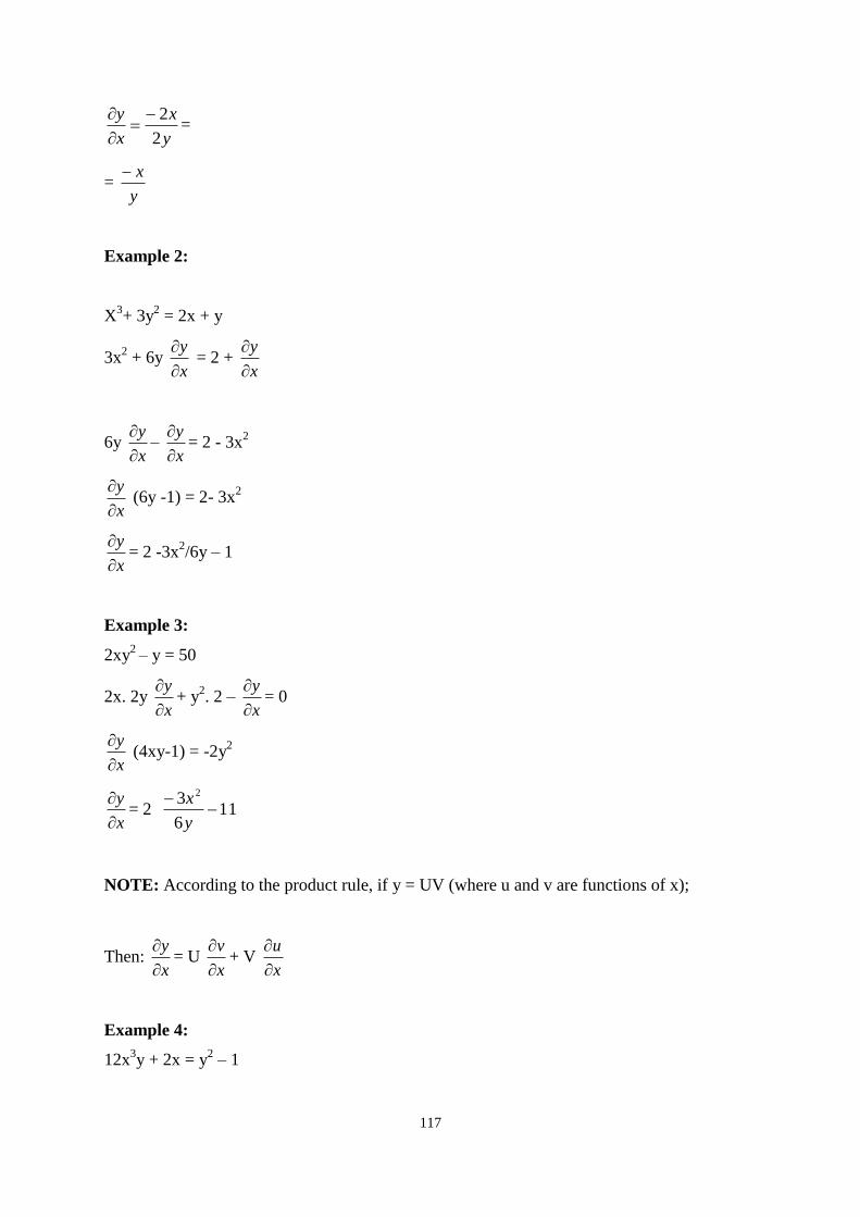
117

y

x

x

y

2

2

=

= y

x

Example 2:

X3+ 3y

2 = 2x + y

3x2 + 6y

x

y

= 2 +

x

y

6y x

y

–

x

y

= 2 - 3x

2

x

y

(6y -1) = 2- 3x

2

x

y

= 2 -3x

2/6y – 1

Example 3:

2xy2

– y = 50

2x. 2y x

y

+ y

2. 2 –

x

y

= 0

x

y

(4xy-1) = -2y

2

x

y

= 2 1

6

3 2

y

x1

NOTE: According to the product rule, if y = UV (where u and v are functions of x);

Then: x

y

= U

x

v

+ V

x

u

Example 4:

12x3y + 2x = y

2 – 1

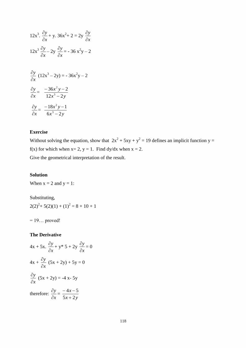
118

12x3.

x

y

+ y. 36x

2+ 2 = 2y

x

y

12x3

x

y

– 2y

x

y

= - 36 x

2y – 2

x

y

(12x

3 – 2y) = - 36x

2y – 2

x

y

=

yx

yx

212

2363

2

x

y

=

yx

yx

26

1183

2

Exercise

Without solving the equation, show that 2x2 + 5xy + y

2 = 19 defines an implicit function y =

f(x) for which when x= 2, y = 1. Find dy/dx when x = 2.

Give the geometrical interpretation of the result.

Solution

When x = 2 and y = 1:

Substituting,

2(2)2+ 5(2)(1) + (1)

2 = 8 + 10 + 1

= 19… proved!

The Derivative

4x + 5x. x

y

+ y* 5 + 2y

x

y

= 0

4x + x

y

(5x + 2y) + 5y = 0

x

y

(5x + 2y) = -4 x- 5y

therefore: x

y

=

yx

x

25

54

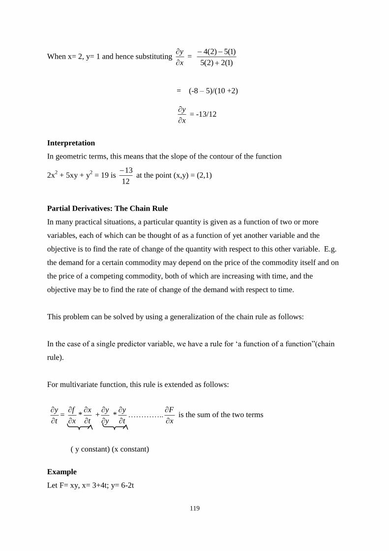
119

When x= 2, y= 1 and hence substituting x

y

=

)1(2)2(5

)1(5)2(4

= (-8 – 5)/(10 +2)

x

y

= -13/12

Interpretation

In geometric terms, this means that the slope of the contour of the function

2x2 + 5xy + y

2 = 19 is

12

13 at the point (x,y) = (2,1)

Partial Derivatives: The Chain Rule

In many practical situations, a particular quantity is given as a function of two or more

variables, each of which can be thought of as a function of yet another variable and the

objective is to find the rate of change of the quantity with respect to this other variable. E.g.

the demand for a certain commodity may depend on the price of the commodity itself and on

the price of a competing commodity, both of which are increasing with time, and the

objective may be to find the rate of change of the demand with respect to time.

This problem can be solved by using a generalization of the chain rule as follows:

In the case of a single predictor variable, we have a rule for ‘a function of a function”(chain

rule).

For multivariate function, this rule is extended as follows:

t

y

=

x

f

*

t

x

+

y

y

*

t

y

…………..

x

F

is the sum of the two terms

( y constant) (x constant)

Example

Let F= xy, x= 3+4t; y= 6-2t

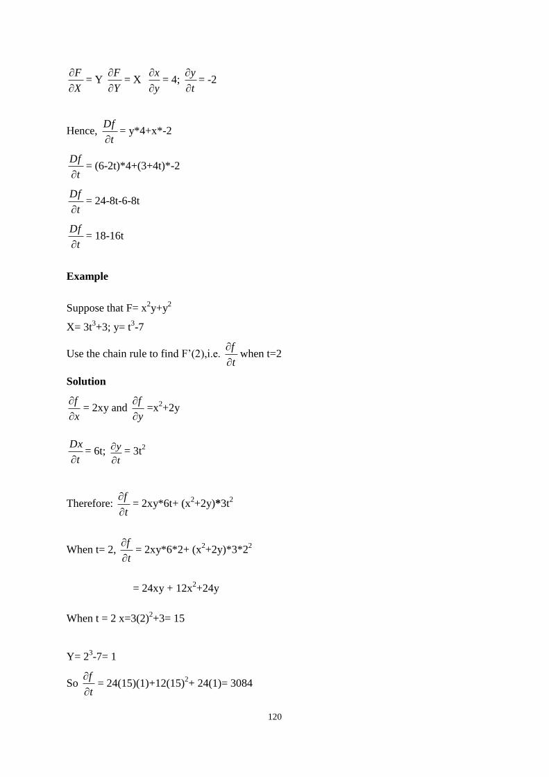
120

X

F

= Y

Y

F

= X

y

x

= 4;

t

y

= -2

Hence, t

Df

= y*4+x*-2

t

Df

= (6-2t)*4+(3+4t)*-2

t

Df

= 24-8t-6-8t

t

Df

= 18-16t

Example

Suppose that F= x2y+y

2

X= 3t3+3; y= t

3-7

Use the chain rule to find F’(2),i.e. t

f

when t=2

Solution

x

f

= 2xy and

y

f

=x

2+2y

t

Dx

= 6t;

t

y

= 3t2

Therefore: t

f

= 2xy*6t+ (x

2+2y)*3t

2

When t= 2, t

f

= 2xy*6*2+ (x

2+2y)*3*2

2

= 24xy + 12x2+24y

When t = 2 x=3(2)2+3= 15

Y= 23-7= 1

So t

f

= 24(15)(1)+12(15)

2+ 24(1)= 3084

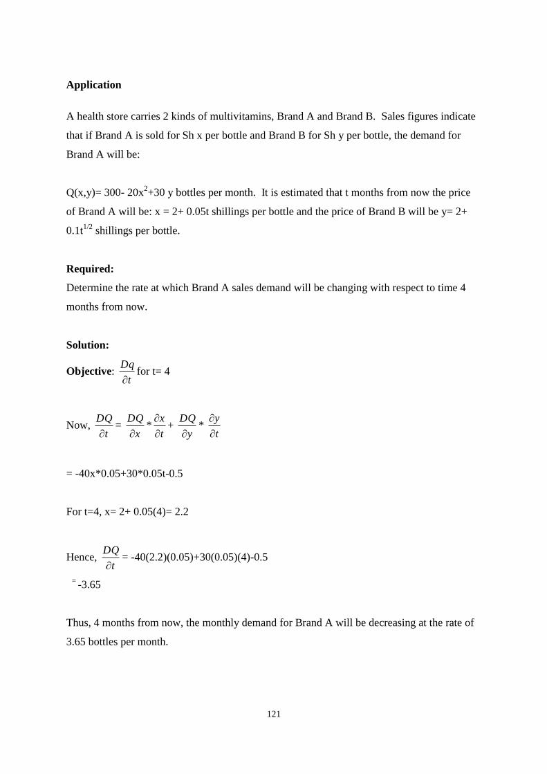
121

Application

A health store carries 2 kinds of multivitamins, Brand A and Brand B. Sales figures indicate

that if Brand A is sold for Sh x per bottle and Brand B for Sh y per bottle, the demand for

Brand A will be:

Q(x,y)= 300- 20x2+30 y bottles per month. It is estimated that t months from now the price

of Brand A will be: x = 2+ 0.05t shillings per bottle and the price of Brand B will be y= 2+

0.1t1/2

shillings per bottle.

Required:

Determine the rate at which Brand A sales demand will be changing with respect to time 4

months from now.

Solution:

Objective: t

Dq

for t= 4

Now, t

DQ

=

x

DQ

*

t

x

+

y

DQ

*

t

y

= -40x*0.05+30*0.05t-0.5

For t=4, x= 2+ 0.05(4)= 2.2

Hence, t

DQ

= -40(2.2)(0.05)+30(0.05)(4)-0.5

= -3.65

Thus, 4 months from now, the monthly demand for Brand A will be decreasing at the rate of

3.65 bottles per month.

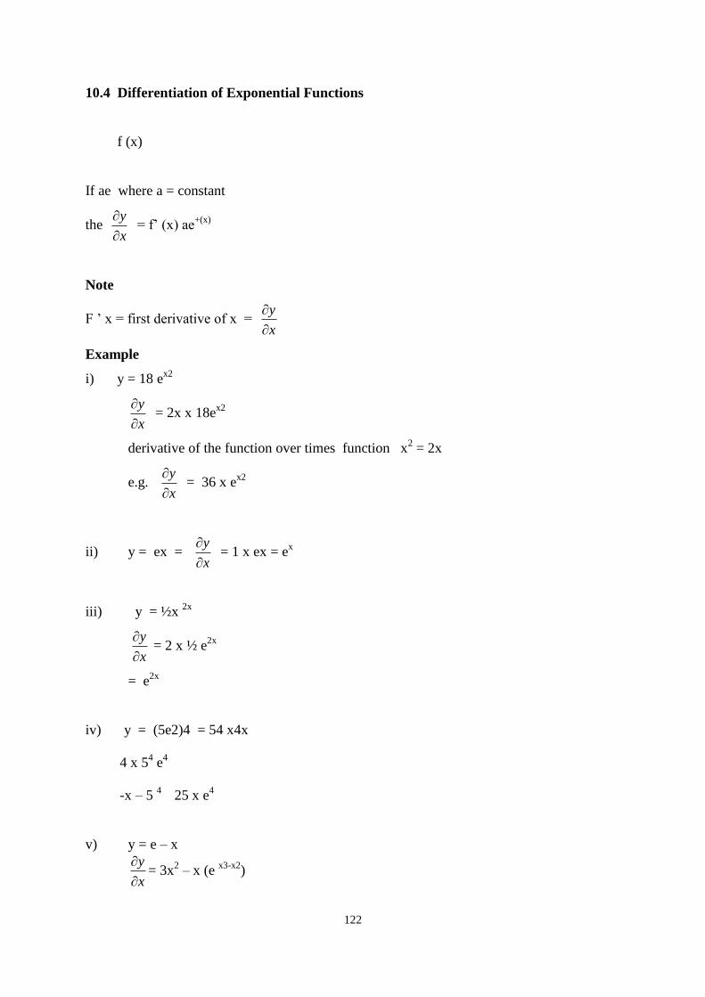
122

10.4 Differentiation of Exponential Functions

f (x)

If ae where a = constant

the x

y

= f’ (x) ae

+(x)

Note

F ’ x = first derivative of x = x

y

Example

i) y = 18 ex2

x

y

= 2x x 18e

x2

derivative of the function over times function x2 = 2x

e.g. x

y

= 36 x e

x2

ii) y = ex = x

y

= 1 x ex = e

x

iii) y = ½x 2x

x

y

= 2 x ½ e

2x

= e2x

iv) y = (5e2)4 = 54 x4x

4 x 54 e

4

-x – 5 4 25 x e

4

v) y = e – x

x

y

= 3x

2 – x (e

x3-x2)

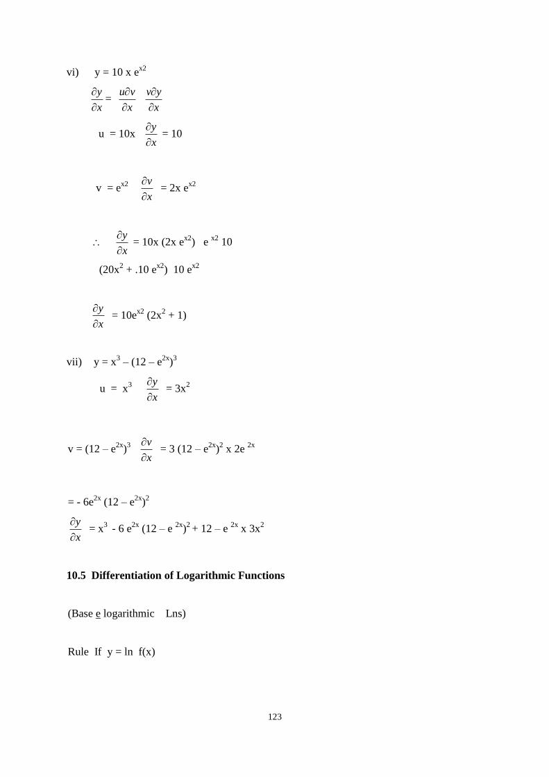
123

vi) y = 10 x ex2

x

y

=

x

vu

x

yv

u = 10x x

y

= 10

v = ex2

x

v

= 2x e

x2

x

y

= 10x (2x e

x2) e

x2 10

(20x2 + .10 e

x2) 10 e

x2

x

y

= 10e

x2 (2x

2 + 1)

vii) y = x3 – (12 – e

2x)3

u = x3

x

y

= 3x

2

v = (12 – e2x

)3

x

v

= 3 (12 – e

2x)2 x 2e

2x

= - 6e2x

(12 – e2x

)2

x

y

= x

3 - 6 e

2x (12 – e

2x)2 + 12 – e

2x x 3x

2

10.5 Differentiation of Logarithmic Functions

(Base e logarithmic Lns)

Rule If y = ln f(x)

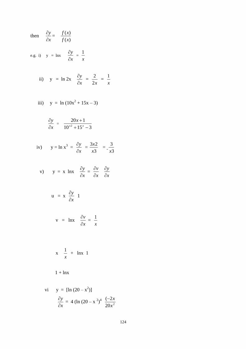
124

then x

y

=

)(

)(

xf

xf

e.g. i) y = lnx x

y

=

x

1

ii) y = ln 2x x

y

=

x2

2 =

x

1

iii) y = ln (10x2 + 15x – 3)

x

y

=

31510

1202

xx

x

iv) y = ln x3 =

x

y

=

3

23

x

x =

3

3

x

v) y = x lnx x

y

=

x

v

x

y

u = x x

y

1

v = lnx x

v

=

x

1

x x

1 + lnx 1

1 + lnx

vi y = [ln (20 – x2)]

x

y

= 4 (ln (20 – x

2)4

220

2(

x

x

125

10.6 Applications (To Add More Material)

10.7

Summary

This lecture extended the concept of differentiation further by considering

functions which cannot be easily expressed in terms of the dependent

variable (implicit functions). Also dealt with is the differentiation of

exponential and logarithmic functions and their uses.

The next lecture will introduce the concept of integration, which is the inverse of

differentiation.

Activity

1. (a) Kiplimo Njoroge Certified Public Accountants have recently started to offer business

advice to their clients. Acting as consultants, they have estimated the demand curve of a

client’s firm to be:

AR = 200 – 8q

Where AR is average revenue in millions of shillings and q is the output in units.

Investigations of the client firm’s profile shows that marginal cost (MC) is given by:

MC = q2

- 28q + 173 (in millions of shillings)

Further investigations have shown that the firm’s fixed cost is Sh. 10 million.

Required:

Determine:

i) Total revenue function,

ii) Total cost function and hence,

iii) The profit function.

(b) What advice would you give the client in terms of production level and price to charge if

its objective is to maximize profit? What is the maximum profit?

(c) Compare the marginal revenue and average cost values when q = 5 units.

126

2. (a) A national record distribution company sells records and tapes by mail only.

Advertising is done on local TV stations. A promotion program is planned for a major

metropolitan area for a new country western album. The target audience-those who might be

interested in this type of album- is estimated at 800,000. Past experience indicates that for

this city and this type of album the percentage of the target market R actually purchasing an

album or tape is a function of the length of the advertising campaign, t. Specifically, this sales

response function is:

R = 1 – e- 0.025t

The profit margin on each album is $ 2.50. Advertising costs include a fixed cost of $ 20,000

and a variable cost of $ 2,500 per day.

Required:

i) Determine how long the campaign should be conducted if the goal is to maximize net

profit (i.e. gross profit minus advertising costs).

ii) What is the expected maximum net profit?

iii) What percentage of the target market is expected to purchase the album?

(b) A company is hiring persons to work in its plant. For the job the persons will perform,

efficiency experts estimate that the average cost C of performing the task is a function of

the number of persons hired, x. Specifically,

C = f(x)= 0.005x2 – 0.49 ln x + 5

Required:

i) Determine the number of persons who should be hired to minimize the average cost.

ii) Given the demand relationship p = 800 – 75 ln q, determine the elasticity of demand when

demand equals 200.

(c) The demand for a particular commodity is given by:

P = 15e-x/3

for 0≤ x≤ 8

Where p = price and x = quantity.

Determine the price and quantity for which revenue is maximum and price elasticity of

demand at that point and interpret it.

127

LECTURE ELEVEN

INTEGRATION

Lecture Outline

11.1 Introduction

11.2 Objectives

11.3 Integration

11.3.1 Indefinite Integration

11.3.2 Definite Integration

11.4 Summary

10.1 Introduction

Welcome to Lecture 11. In lectures 6 up to 10, we have been studying differentiation. In this

lecture, we begin the study and applications of integration, which is the inverse of

differentiation.

Objectives

At the end of this lecture, you should be able to:4

1. Recognize the notation for integration.

2. Write down the integrals of functions.

3. Evaluate definite integrals.

4. Apply integration in solving business problems.

11.3 Integration

Integration has two interpretations.

1. As a procedure which is the inverse of differentiation. [known as indefinite integration]

2. As a means of obtaining the area under a curve [known as definite integration]

11.3.1 Indefinite Integration:

This involves finding the anti-derivative of a function if we know its derivative.

Usual Question "What function which when differentiated yields to this derivative?"

11.2

128

Examples:

1. x

y

= 3x

2 then y = x

3

2. x

y

= 2x then y = x

2

Symbols of integration: ∫ elongated 'S')

1. ∫ 3x2 x = x

3

2. 22 xxx

Constant of integration:

For any integral, an arbitrary constant has to be added since the derivative of a constant is

zero

e.g. i) y = x3

x

y

= 3x

2

ii) y = x3 + 24

x

y

= 3x

2

iii) y = x3 - 154

x

y

= 3x

2

Since its not possible to know which function had been differentiated in order to obtain

23xx

y

It is necessary to add a constant to the integral as follows:

If x

y

= 3x

2 Then y = 323 xxx xx23 y = x

3 + c where c is a constant.

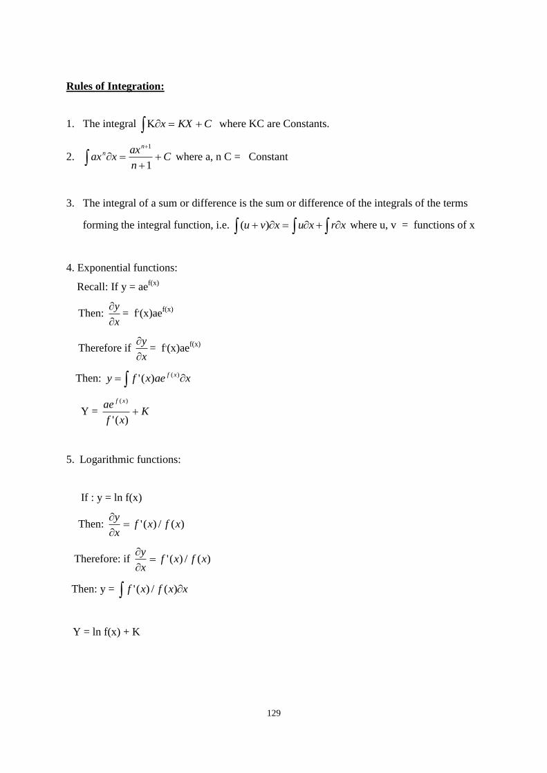
129

Rules of Integration:

1. The integral CKXx where KC are Constants.

2. Cn

axxax

nn

1

1

where a, n C = Constant

3. The integral of a sum or difference is the sum or difference of the integrals of the terms

forming the integral function, i.e. xvu )( xrxu where u, v = functions of x

4. Exponential functions:

Recall: If y = aef(x)

Then: x

y

= f

,(x)ae

f(x)

Therefore if x

y

= f

,(x)ae

f(x)

Then: xaexfy xf )()('

Y = Kxf

ae xf

)('

)(

5. Logarithmic functions:

If : y = ln f(x)

Then: )(/)(' xfxfx

y

Therefore: if )(/)(' xfxfx

y

Then: y = xxfxf )(/)('

Y = ln f(x) + K

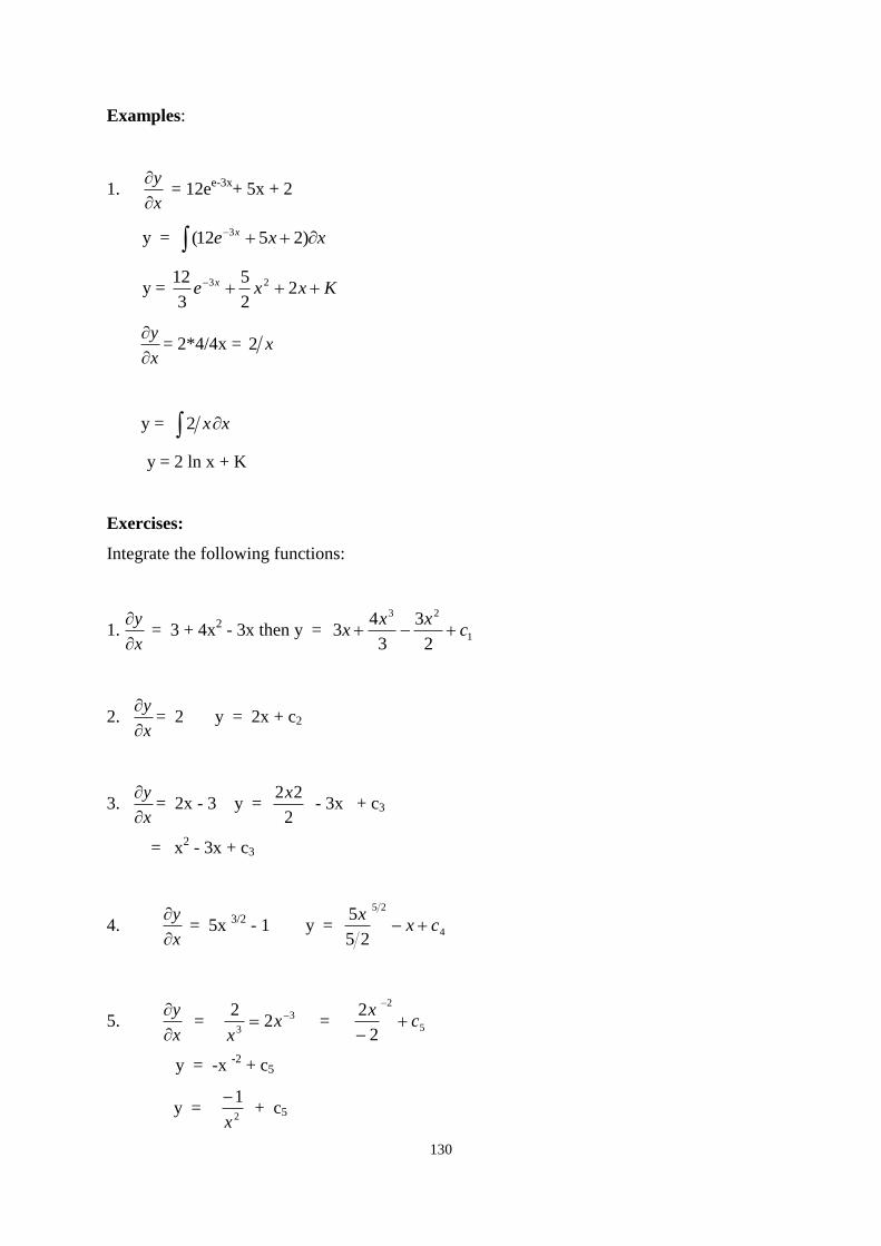
130

Examples:

1. x

y

= 12e

e-3x+ 5x + 2

y = xxe x )2512( 3

y = Kxxe x 22

5

3

12 23

x

y

= 2*4/4x = x2

y = xx2

y = 2 ln x + K

Exercises:

Integrate the following functions:

1. x

y

= 3 + 4x

2 - 3x then y = 1

23

2

3

3

43 c

xxx

2. x

y

= 2 y = 2x + c2

3. x

y

= 2x - 3 y =

2

22x - 3x + c3

= x2 - 3x + c3

4. x

y

= 5x

3/2 - 1 y = 4

25

25

5cx

x

5. x

y

= 3

32

2 xx

= 5

2

2

2c

x

y = -x -2

+ c5

y = 2

1

x

+ c5

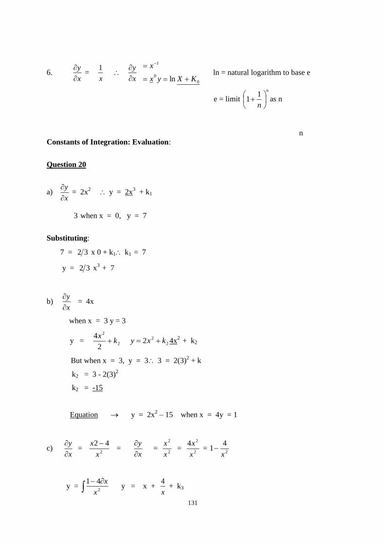
131

6. x

y

=

x

1

x

y

0

0

1

ln KXyx

x

ln = natural logarithm to base e

e = limit

n

n

11 as n

n

Constants of Integration: Evaluation:

Question 20

a) x

y

= 2x

2 y = 2x

3 + k1

3 when x = 0, y = 7

Substituting:

7 = 32 x 0 + k1 k1 = 7

y = 32 x3

+ 7

b) x

y

= 4x

when x = 3 y = 3

y = 2

2

2

2

22

4kxyk

x 4x

2 + k2

But when x = 3, y = 3 3 = 2(3)2 + k

k2 = 3 - 2(3)2

k2 = -15

Equation y = 2x2 – 15 when x = 4y = 1

c) x

y

=

2

42

x

x =

x

y

=

2

2

x

x =

2

24

x

x =

2

41

x

y =

2

41

x

x y = x +

x

4 + k3

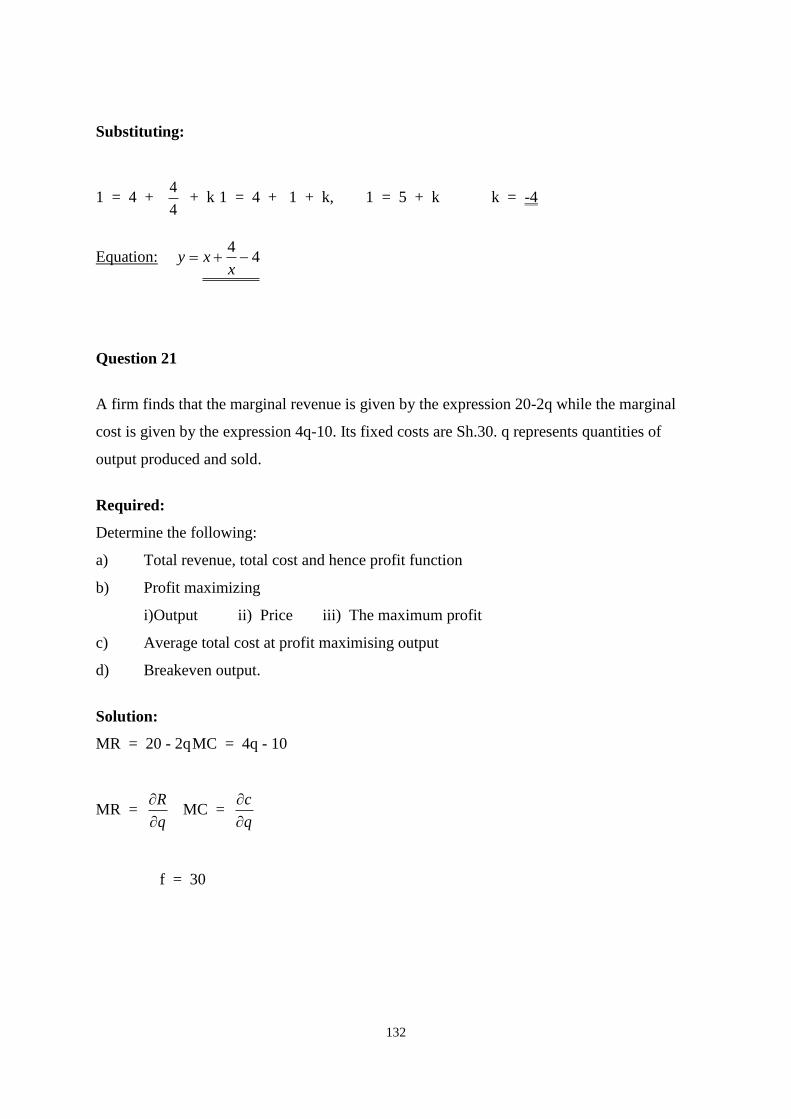
132

Substituting:

1 = 4 + 4

4 + k 1 = 4 + 1 + k, 1 = 5 + k k = -4

Equation: 44

xxy

Question 21

A firm finds that the marginal revenue is given by the expression 20-2q while the marginal

cost is given by the expression 4q-10. Its fixed costs are Sh.30. q represents quantities of

output produced and sold.

Required:

Determine the following:

a) Total revenue, total cost and hence profit function

b) Profit maximizing

i) Output ii) Price iii) The maximum profit

c) Average total cost at profit maximising output

d) Breakeven output.

Solution:

MR = 20 - 2q MC = 4q - 10

MR = q

R

MC =

q

c

f = 30

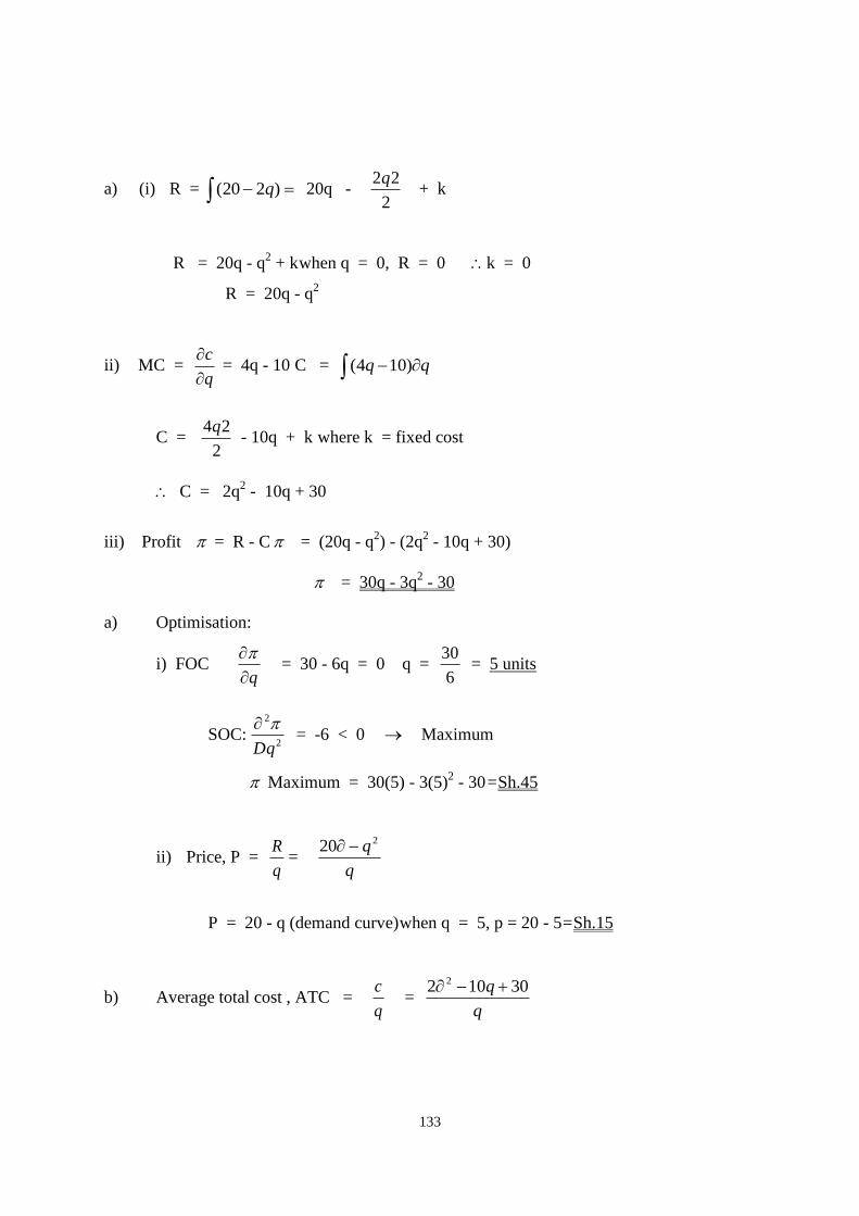
133

a) (i) R = )220( q 20q - 2

22q + k

R = 20q - q2 + k when q = 0, R = 0 k = 0

R = 20q - q2

ii) MC = q

c

= 4q - 10 C = qq )104(

C = 2

24q- 10q + k where k = fixed cost

C = 2q2 - 10q + 30

iii) Profit = R - C = (20q - q2) - (2q

2 - 10q + 30)

= 30q - 3q2 - 30

a) Optimisation:

i) FOC q

= 30 - 6q = 0 q =

6

30 = 5 units

SOC: 2

2

Dq

= -6 < 0 Maximum

Maximum = 30(5) - 3(5)2 - 30 = Sh.45

ii) Price, P = q

R =

q

q 220

P = 20 - q (demand curve) when q = 5, p = 20 - 5 = Sh.15

b) Average total cost , ATC = q

c =

q

q 30102 2

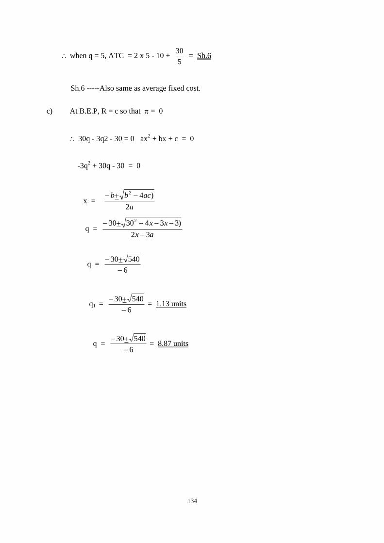
134

when q = 5, ATC = 2 x 5 - 10 + 5

30 = Sh.6

Sh.6 -----Also same as average fixed cost.

c) At B.E.P, R = c so that = 0

30q - 3q2 - 30 = 0 ax2 + bx + c = 0

-3q2 + 30q - 30 = 0

x = a

acbb

2

)42

q = ax

xx

32

)3343030 2

q = 6

54030

q1 = 6

54030

= 1.13 units

q = 6

54030

= 8.87 units

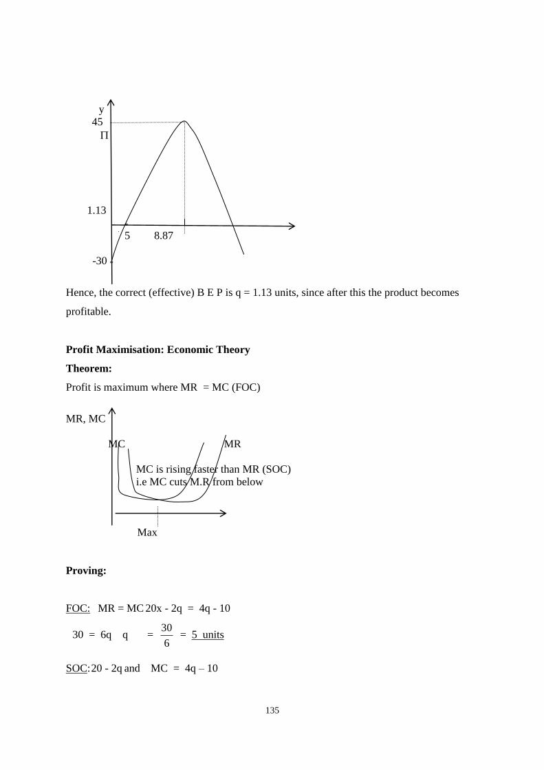
135

y

45

1.13

*

5 8.87

-30 *

Hence, the correct (effective) B E P is q = 1.13 units, since after this the product becomes

profitable.

Profit Maximisation: Economic Theory

Theorem:

Profit is maximum where MR = MC (FOC)

MR, MC

MC MR

MC is rising faster than MR (SOC)

i.e MC cuts M.R from below

Max

Proving:

FOC: MR = MC 20x - 2q = 4q - 10

30 = 6q q = 6

30 = 5 units

SOC: 20 - 2q and MC = 4q – 10

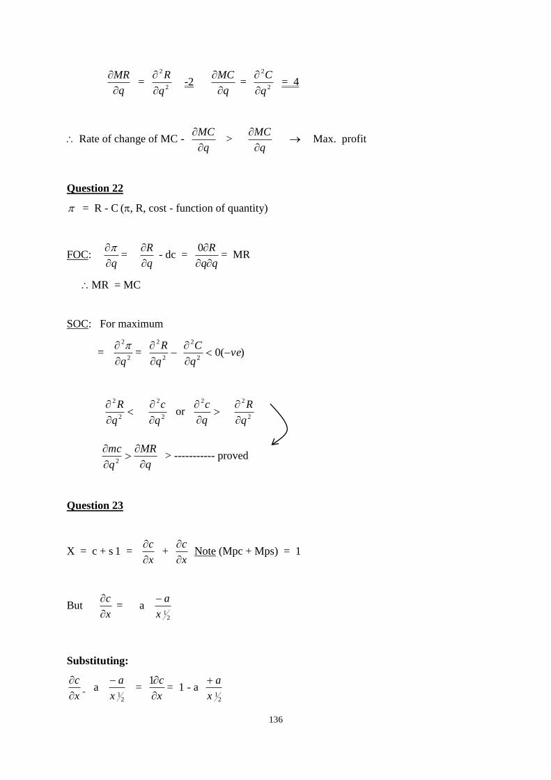
136

q

MR

=

2

2

q

R

-2

q

MC

=

2

2

q

C

= 4

Rate of change of MC - q

MC

>

q

MC

Max. profit

Question 22

= R - C (, R, cost - function of quantity)

FOC: q

=

q

R

- dc =

qq

R

0= MR

MR = MC

SOC: For maximum

= 2

2

q

=

2

2

q

R )(0

2

2

veq

C

2

2

q

R

2

2

q

c

or

q

c2

2

2

q

R

q

MR

q

mc

2

> ----------- proved

Question 23

X = c + s 1 = x

c

+

x

c

Note (Mpc + Mps) = 1

But x

c

= a

21x

a

Substituting:

x

c

a

21x

a =

x

c

1= 1 - a

21x

a

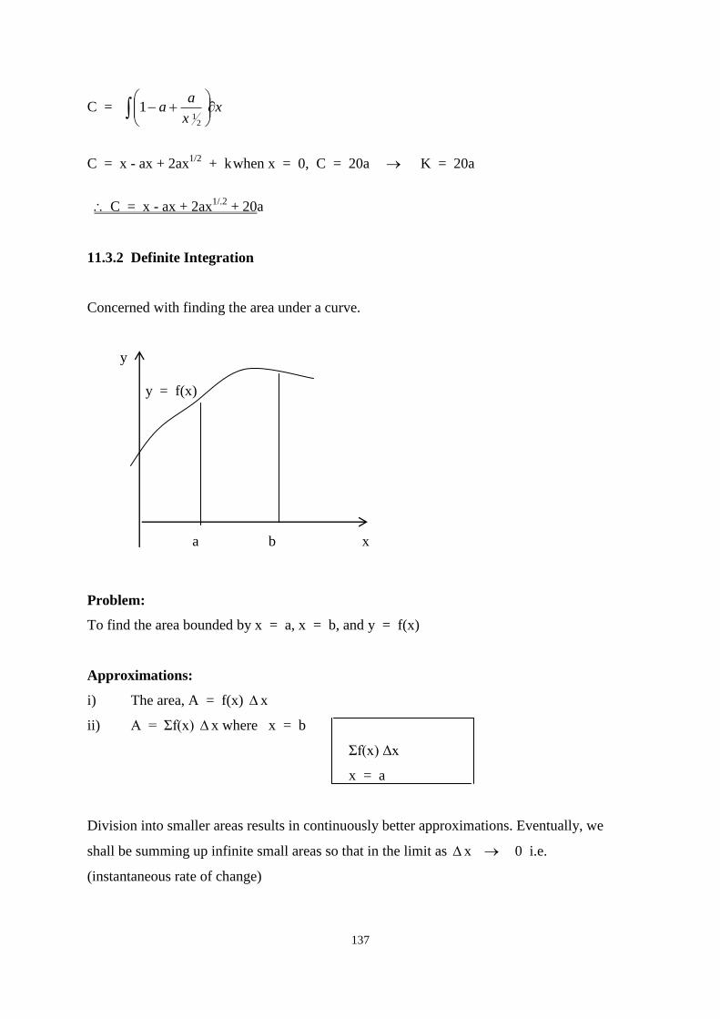
137

C = xx

aa

21

1

C = x - ax + 2ax1/2

+ k when x = 0, C = 20a K = 20a

C = x - ax + 2ax1/.2

+ 20a

11.3.2 Definite Integration

Concerned with finding the area under a curve.

y

y = f(x)

a b x

Problem:

To find the area bounded by x = a, x = b, and y = f(x)

Approximations:

i) The area, A = f(x) x

ii) A = Σf(x) x where x = b

Σf(x) Δx

x = a

Division into smaller areas results in continuously better approximations. Eventually, we

shall be summing up infinite small areas so that in the limit as x 0 i.e.

(instantaneous rate of change)

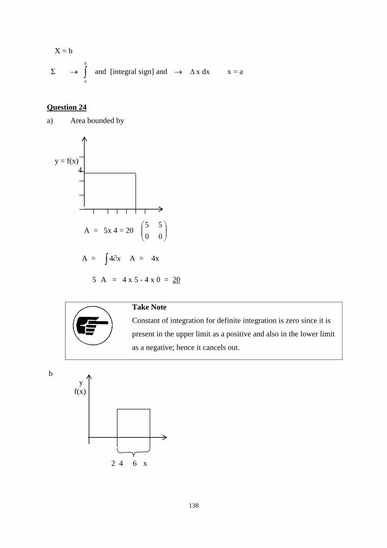
138

X = b

Σ b

a

and [integral sign] and x dx x = a

Question 24

a) Area bounded by

y = f(x)

4

A = 5x 4 = 20

0

5

0

5

A = x4 A = 4x

5 A = 4 x 5 - 4 x 0 = 20

Take Note

Constant of integration for definite integration is zero since it is

present in the upper limit as a positive and also in the lower limit

as a negative; hence it cancels out.

b

y

f(x)

2 4 6 x

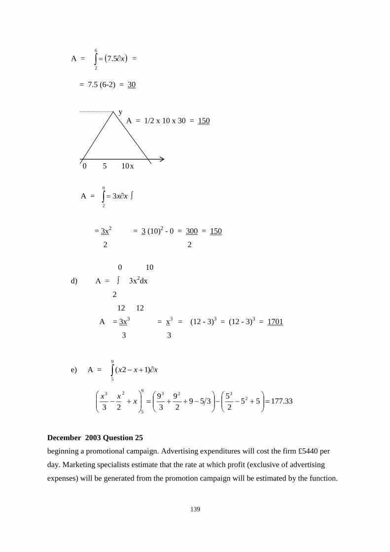
139

A =

6

2

5.7 x =

= 7.5 (6-2) = 30

y

A = 1/2 x 10 x 30 = 150

0 5 10 x

A =

0

2

3 xx ∫

= 3x2 = 3 (10)

2 - 0 = 300 = 150

2 2

0 10

d) A = ∫ 3x2dx

2

12 12

A = 3x3 = x

3 = (12 - 3)

3 = (12 - 3)

3 = 1701

3 3

e) A =

9

5

)12( xxx

33.177552

5359

2

9

3

9

23

2323

9

5

23

x

xx

December 2003 Question 25

beginning a promotional campaign. Advertising expenditures will cost the firm £5440 per

day. Marketing specialists estimate that the rate at which profit (exclusive of advertising

expenses) will be generated from the promotion campaign will be estimated by the function.

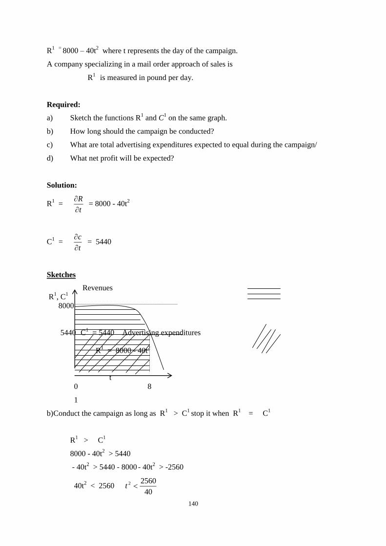
140

R1 =

8000 – 40t2 where t represents the day of the campaign.

A company specializing in a mail order approach of sales is

R1

is measured in pound per day.

Required:

a) Sketch the functions R1 and C

1 on the same graph.

b) How long should the campaign be conducted?

c) What are total advertising expenditures expected to equal during the campaign/

d) What net profit will be expected?

Solution:

R1 =

t

R

= 8000 - 40t

2

C1 =

t

c

= 5440

Sketches

Revenues

R1, C

1

8000

5440 C1 = 5440 Advertising expenditures

R1 = 8000 - 40t

2

t

0 8

1

b) Conduct the campaign as long as R1 > C

1 stop it when R

1 = C

1

R1 > C

1

8000 - 40t2 > 5440

- 40t2 > 5440 - 8000 - 40t

2 > -2560

40t2 < 2560

40

25602 t

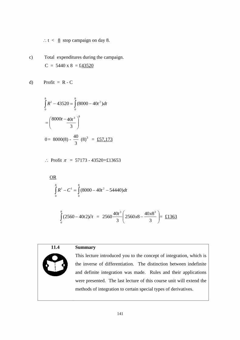
141

t < 8 stop campaign on day 8.

c) Total expenditures during the campaign.

C = 5440 x 8 = £43520

d) Profit = R - C

8

0

2

8

0

1 )408000(43520 dttR

83

3

408000

tt

0 = 8000(8) - 3

40 (8)

3 = £57,173

Profit = 57173 - 43520 = £13653

OR

8

0

2

8

0

11 )54440408000( dttCR

8

0

)2402560( tt =

3

84082560

3

402560

33 xx

t= £1363

11.4

Summary

This lecture introduced you to the concept of integration, which is

the inverse of differentiation. The distinction between indefinite

and definite integration was made. Rules and their applications

were presented. The last lecture of this course unit will extend the

methods of integration to certain special types of derivatives.

142

LECTURE TWELVE

MATRICES

Lecture Outlines

12.1 Background

12.2 Objectives

12.3 Introduction to Matrix Algebra

12.3.1 Types of matrices

12.3.2 Matrix Operations

12.4 Summary

12.1 Background

Welcome to Lecture 12 in this course unit. In this lecture we are going to learn about

matrices. Matrices are widely used in business management. Consequently, the lecture will

have two parts.

The first part will cover introduction to matrices and the basic matrix operations while the

second part will focus on their application to business.

12.2 Objectives

At the end of this lecture you should be able to:

1. Define and explain the various types of matrices

2. Undertake basic operations of matrix algebra including addition,

subtraction, multiplication and inversion of matrices.

3. Apply matrix algebra in the solution of simultaneous linear

equations.

4. Evaluate the use of matrix algebra in various managerial situations,

such as:

- Inventory Management

- Markov processes

- Input/output analysis

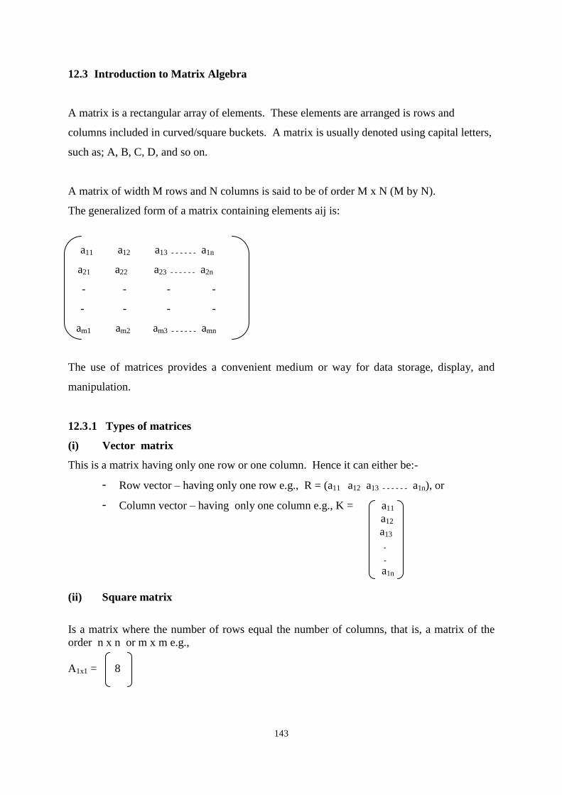
143

12.3 Introduction to Matrix Algebra

A matrix is a rectangular array of elements. These elements are arranged is rows and

columns included in curved/square buckets. A matrix is usually denoted using capital letters,

such as; A, B, C, D, and so on.

A matrix of width M rows and N columns is said to be of order M x N (M by N).

The generalized form of a matrix containing elements aij is:

a11 a12 a13 - - - - - - a1n

a21 a22 a23 - - - - - - a2n

- - - -

- - - -

am1 am2 am3 - - - - - - amn

The use of matrices provides a convenient medium or way for data storage, display, and

manipulation.

12.3 .1 Types of matrices

(i) Vector matrix

This is a matrix having only one row or one column. Hence it can either be:-

- Row vector – having only one row e.g., R = (a11 a12 a13 - - - - - - a1n), or

- Column vector – having only one column e.g., K = a11

a12

a13

-

-

a1n

(ii) Square matrix

Is a matrix where the number of rows equal the number of columns, that is, a matrix of the

order n x n or m x m e.g.,

A1x1 = 8

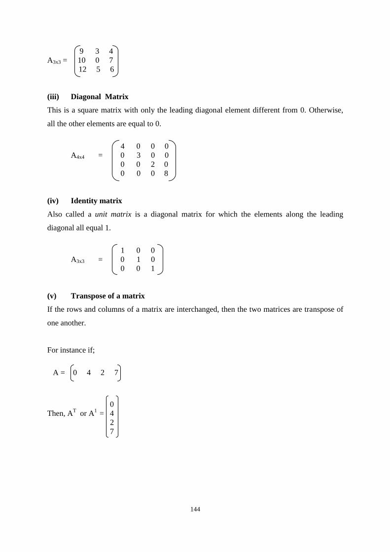
144

9 3 4

A3x3 = 10 0 7

12 5 6

(iii) Diagonal Matrix

This is a square matrix with only the leading diagonal element different from 0. Otherwise,

all the other elements are equal to 0.

4 0 0 0

A4x4 = 0 3 0 0

0 0 2 0

0 0 0 8

(iv) Identity matrix

Also called a unit matrix is a diagonal matrix for which the elements along the leading

diagonal all equal 1.

1 0 0

A3x3 = 0 1 0

0 0 1

(v) Transpose of a matrix

If the rows and columns of a matrix are interchanged, then the two matrices are transpose of

one another.

For instance if;

A = 0 4 2 7

0

Then, AT or A

1 = 4

2

7

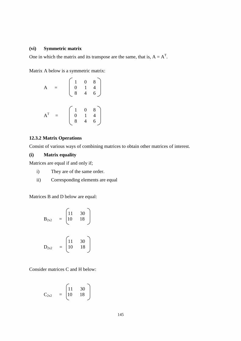
145

(vi) Symmetric matrix

One in which the matrix and its transpose are the same, that is, A = AT.

Matrix A below is a symmetric matrix:

1 0 8

A = 0 1 4

8 4 6

1 0 8

AT = 0 1 4

8 4 6

12.3.2 Matrix Operations

Consist of various ways of combining matrices to obtain other matrices of interest.

(i) Matrix equality

Matrices are equal if and only if;

i) They are of the same order.

ii) Corresponding elements are equal

Matrices B and D below are equal:

11 30

B2x2 = 10 18

11 30

D2x2 = 10 18

Consider matrices C and H below:

11 30

C2x2 = 10 18

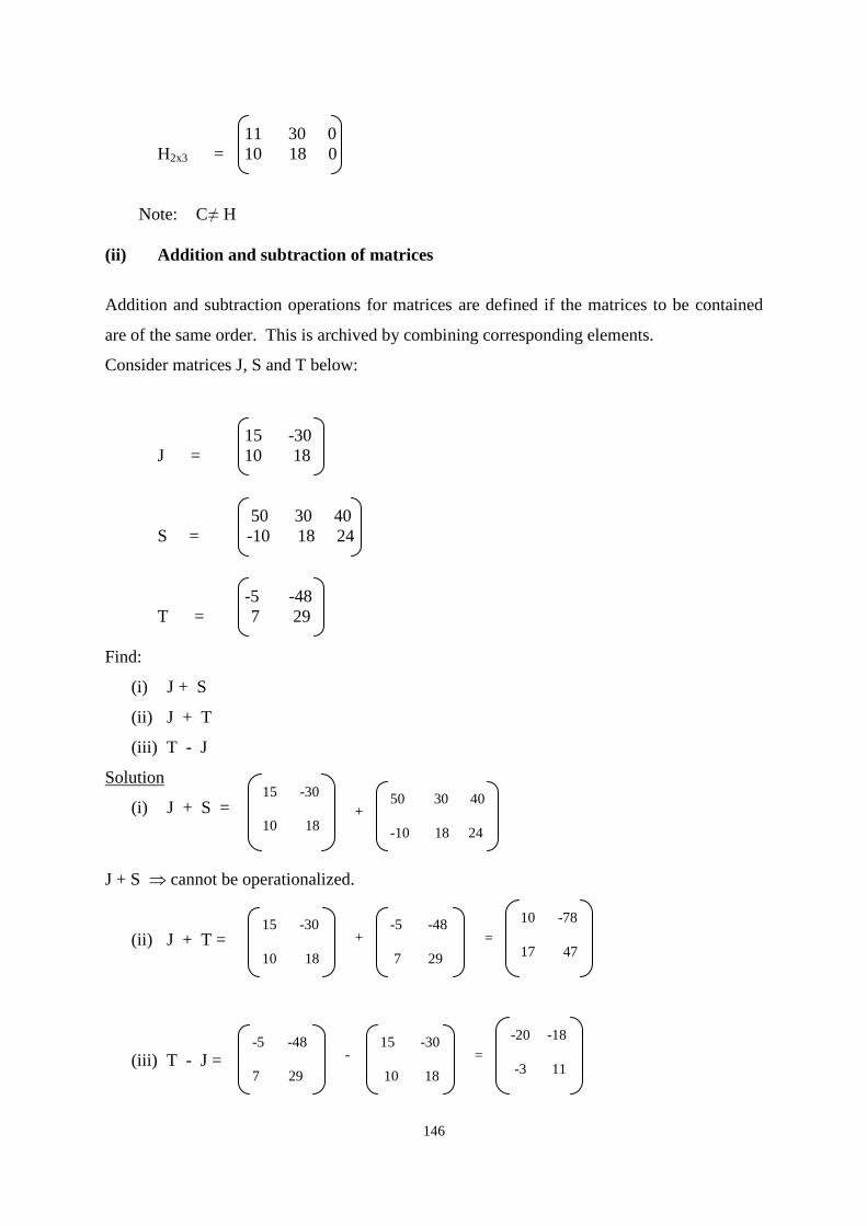
146

11 30 0

H2x3 = 10 18 0

Note: C ≠ H

(ii) Addition and subtraction of matrices

Addition and subtraction operations for matrices are defined if the matrices to be contained

are of the same order. This is archived by combining corresponding elements.

Consider matrices J, S and T below:

15 -30

J = 10 18

50 30 40

S = -10 18 24

-5 -48

T = 7 29

Find:

(i) J + S

(ii) J + T

(iii) T - J

Solution

(i) J + S =

J + S cannot be operationalized.

(ii) J + T =

(iii) T - J =

15 -30

10 18

50 30 40

-10 18 24

+

15 -30

10 18

-5 -48

7 29

+ = 10 -78

17 47

-5 -48

7 29

15 -30

10 18

- = -20 -18

-3 11

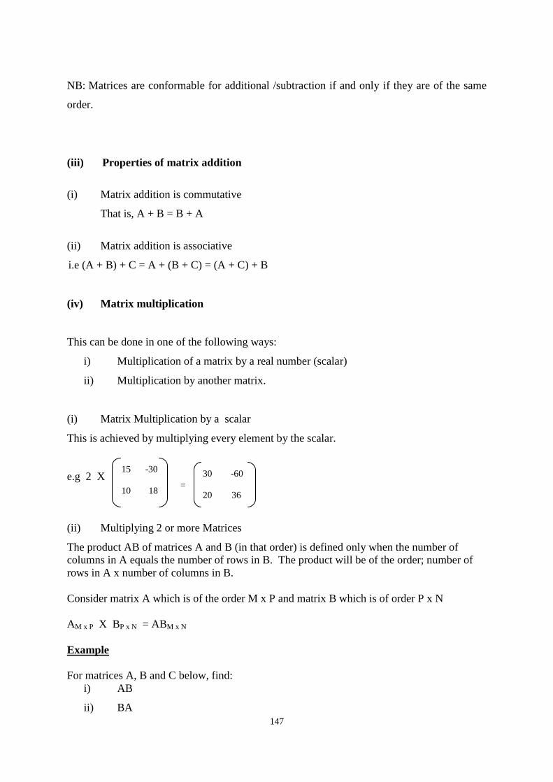
147

NB: Matrices are conformable for additional /subtraction if and only if they are of the same

order.

(iii) Properties of matrix addition

(i) Matrix addition is commutative

That is, A + B = B + A

(ii) Matrix addition is associative

i.e (A + B) + C = A + (B + C) = (A + C) + B

(iv) Matrix multiplication

This can be done in one of the following ways:

i) Multiplication of a matrix by a real number (scalar)

ii) Multiplication by another matrix.

(i) Matrix Multiplication by a scalar

This is achieved by multiplying every element by the scalar.

e.g 2 X

(ii) Multiplying 2 or more Matrices

The product AB of matrices A and B (in that order) is defined only when the number of

columns in A equals the number of rows in B. The product will be of the order; number of

rows in A x number of columns in B.

Consider matrix A which is of the order M x P and matrix B which is of order P x N

AM x P X BP x N = ABM x N

Example

For matrices A, B and C below, find:

i) AB

ii) BA

15 -30

10 18

30 -60

20 36

=

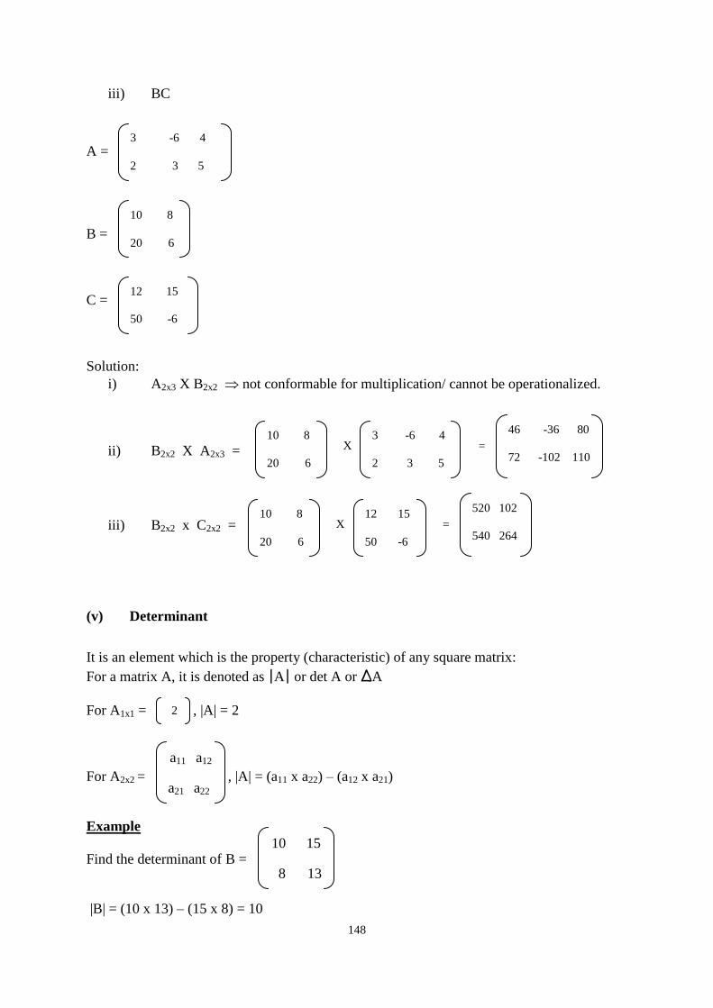
148

iii) BC

A =

B =

C =

Solution:

i) A2x3 X B2x2 not conformable for multiplication/ cannot be operationalized.

ii) B2x2 X A2x3 =

iii) B2x2 x C2x2 =

(v) Determinant

It is an element which is the property (characteristic) of any square matrix:

For a matrix A, it is denoted as |A| or det A or ∆A

For A1x1 = , |A| = 2

For A2x2 = , |A| = (a11 x a22) – (a12 x a21)

Example

Find the determinant of B =

|B| = (10 x 13) – (15 x 8) = 10

3 -6 4

2 3 5

12 15

50 -6

10 8

20 6

12 15

50 -6

X = 520 102

540 264

10 8

20 6

3 -6 4

2 3 5

X = 46 -36 80

72 -102 110

2

a11 a12

a21 a22

10 15

8 13

10 8

20 6

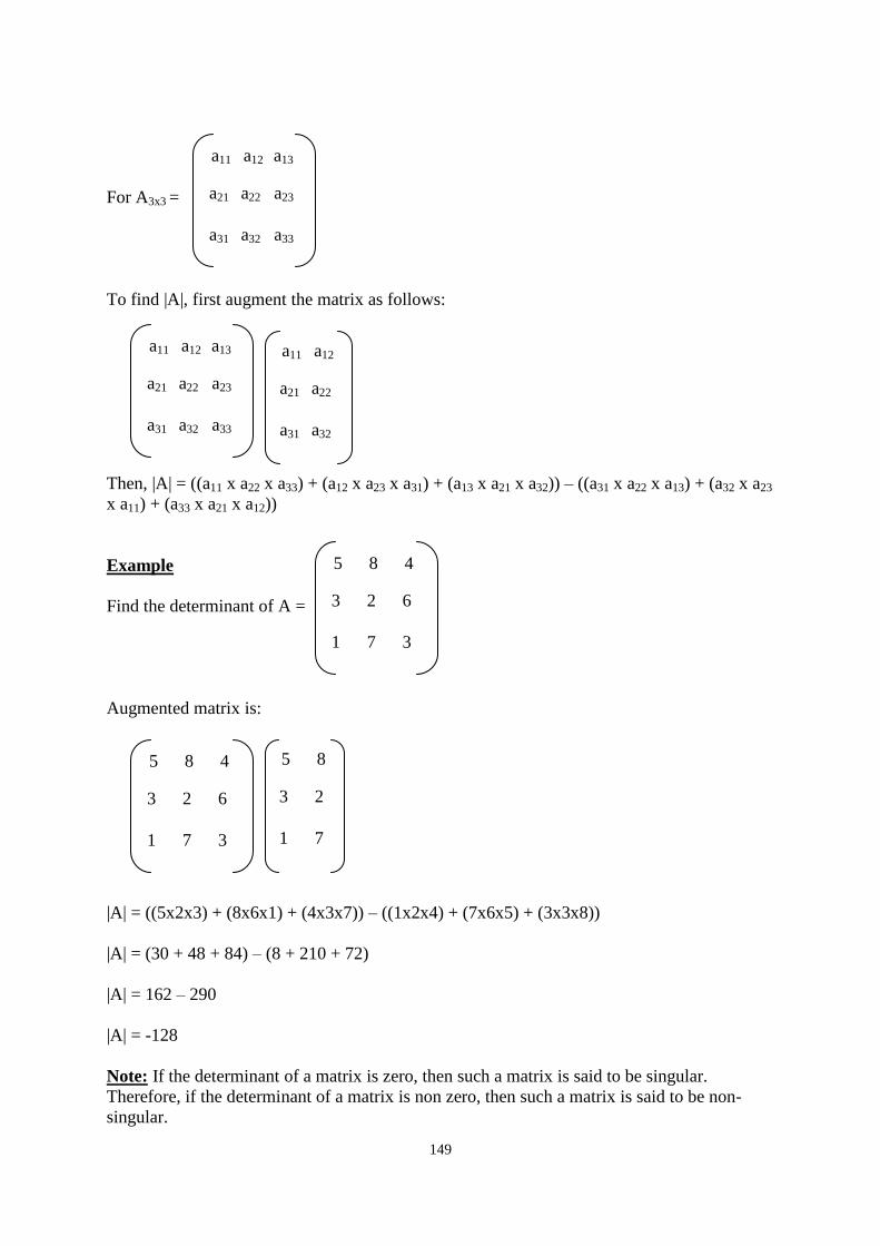
149

For A3x3 =

To find |A|, first augment the matrix as follows:

Then, |A| = ((a11 x a22 x a33) + (a12 x a23 x a31) + (a13 x a21 x a32)) – ((a31 x a22 x a13) + (a32 x a23

x a11) + (a33 x a21 x a12))

Example

Find the determinant of A =

Augmented matrix is:

|A| = ((5x2x3) + (8x6x1) + (4x3x7)) – ((1x2x4) + (7x6x5) + (3x3x8))

|A| = (30 + 48 + 84) – (8 + 210 + 72)

|A| = 162 – 290

|A| = -128

Note: If the determinant of a matrix is zero, then such a matrix is said to be singular.

Therefore, if the determinant of a matrix is non zero, then such a matrix is said to be non-

singular.

a11 a12 a13

a21 a22 a23

a31 a32 a33

a11 a12 a13

a21 a22 a23

a31 a32 a33

a11 a12

a21 a22

a31 a32

5 8 4

3 2 6

1 7 3

5 8 4

3 2 6

1 7 3

5 8

3 2

1 7

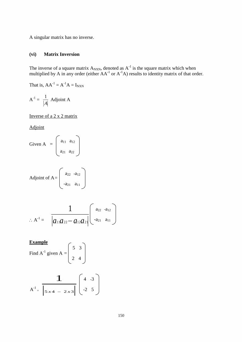
150

A singular matrix has no inverse.

(vi) Matrix Inversion

The inverse of a square matrix ANXN, denoted as A-1

is the square matrix which when

multiplied by A in any order (either AA-1

or A-1

A) results to identity matrix of that order.

That is, AA-1

= A-1

A = INXN

A-1

= A

1 Adjoint A

Inverse of a 2 x 2 matrix

Adjoint

Given A =

Adjoint of A =

A-1

= 21122211

1

aaaa

Example

Find A-1

given A =

A-1

= 3245

1

xx

a11 a12

a21 a22

a22 -a12

-a21 a11

5 3

2 4

4 -3

-2 5

a22 -a12

-a21 a11

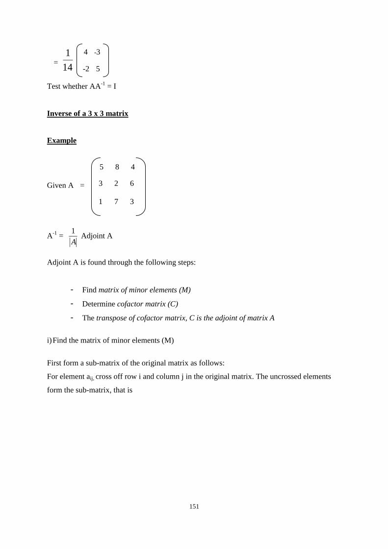
151

= 14

1

Test whether AA-1

= I

Inverse of a 3 x 3 matrix

Example

Given A =

A-1

= A

1 Adjoint A

Adjoint A is found through the following steps:

- Find matrix of minor elements (M)

- Determine cofactor matrix (C)

- The transpose of cofactor matrix, C is the adjoint of matrix A

i) Find the matrix of minor elements (M)

First form a sub-matrix of the original matrix as follows:

For element aij, cross off row i and column j in the original matrix. The uncrossed elements

form the sub-matrix, that is

4 -3

-2 5

5 8 4

3 2 6

1 7 3

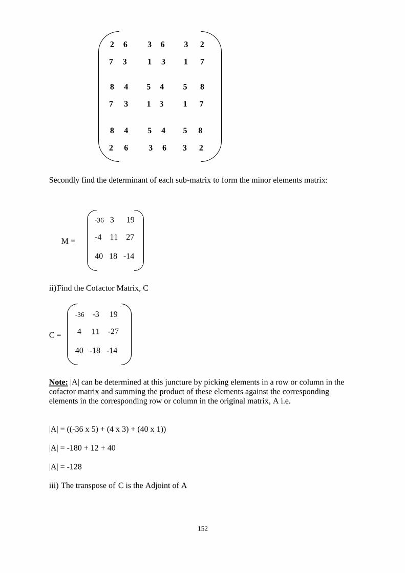
152

Secondly find the determinant of each sub-matrix to form the minor elements matrix:

M =

ii) Find the Cofactor Matrix, C

C =

Note: |A| can be determined at this juncture by picking elements in a row or column in the

cofactor matrix and summing the product of these elements against the corresponding

elements in the corresponding row or column in the original matrix, A i.e.

|A| = ((-36 x 5) + (4 x 3) + (40 x 1))

|A| = -180 + 12 + 40

|A| = -128

iii) The transpose of C is the Adjoint of A

-36 3 19

-4 11 27

40 18 -14

-36 -3 19

4 11 -27

40 -18 -14

2 6 3 6 3 2

7 3 1 3 1 7

8 4 5 4 5 8

7 3 1 3 1 7

8 4 5 4 5 8

2 6 3 6 3 2

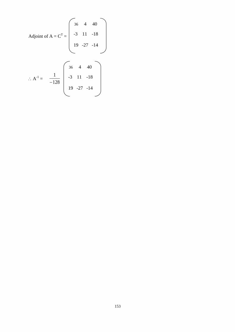
153

Adjoint of A = CT =

A-1

= 128

1

36 4 40

-3 11 -18

19 -27 -14

36 4 40

-3 11 -18

19 -27 -14

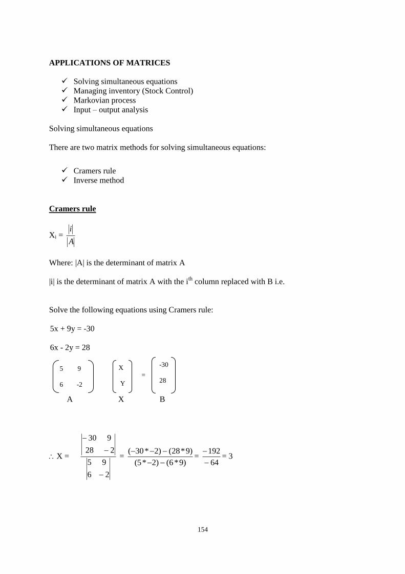
154

APPLICATIONS OF MATRICES

Solving simultaneous equations

Managing inventory (Stock Control)

Markovian process

Input – output analysis

Solving simultaneous equations

There are two matrix methods for solving simultaneous equations:

Cramers rule

Inverse method

Cramers rule

Xi = A

i

Where: |A| is the determinant of matrix A

|i| is the determinant of matrix A with the ith

column replaced with B i.e.

Solve the following equations using Cramers rule:

5x + 9y = -30

6x - 2y = 28

A X B

X =

26

95

228

930

= )9*6()2*5(

)9*28()2*30(

=

64

192

= 3

= 5 9

6 -2

X

Y

-30

28

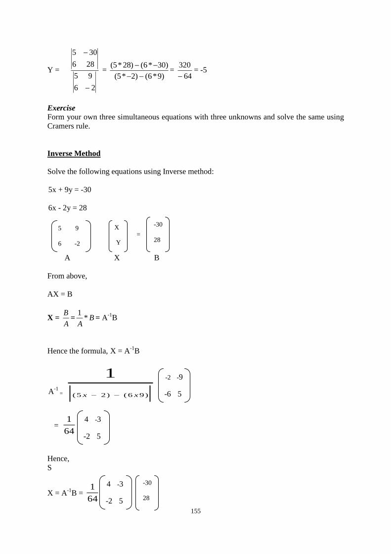
155

Y =

26

95

286

305

= )9*6()2*5(

)30*6()28*5(

=

64

320

= -5

Exercise

Form your own three simultaneous equations with three unknowns and solve the same using

Cramers rule.

Inverse Method

Solve the following equations using Inverse method:

5x + 9y = -30

6x - 2y = 28

A X B

From above,

AX = B

X = A

B= B

A*

1= A

-1B

Hence the formula, X = A-1

B

A-1

= )96()25(

1

xx

= 64

1

Hence,

S

X = A-1

B = 64

1

=

-2 -9

-6 5

4 -3

-2 5

4 -3

-2 5

5 9

6 -2

X

Y

-30

28

-30

28

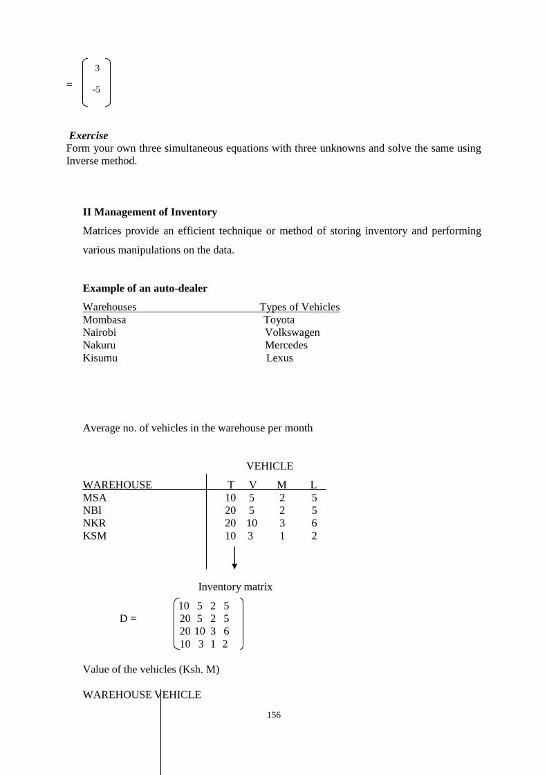
156

=

Exercise

Form your own three simultaneous equations with three unknowns and solve the same using

Inverse method.

II Management of Inventory

Matrices provide an efficient technique or method of storing inventory and performing

various manipulations on the data.

Example of an auto-dealer

Warehouses Types of Vehicles

Mombasa Toyota

Nairobi Volkswagen

Nakuru Mercedes

Kisumu Lexus

Average no. of vehicles in the warehouse per month

VEHICLE

WAREHOUSE T V M L

MSA 10 5 2 5

NBI 20 5 2 5

NKR 20 10 3 6

KSM 10 3 1 2

Inventory matrix

10 5 2 5

D = 20 5 2 5

20 10 3 6

10 3 1 2

Value of the vehicles (Ksh. M)

WAREHOUSE VEHICLE

3

-5

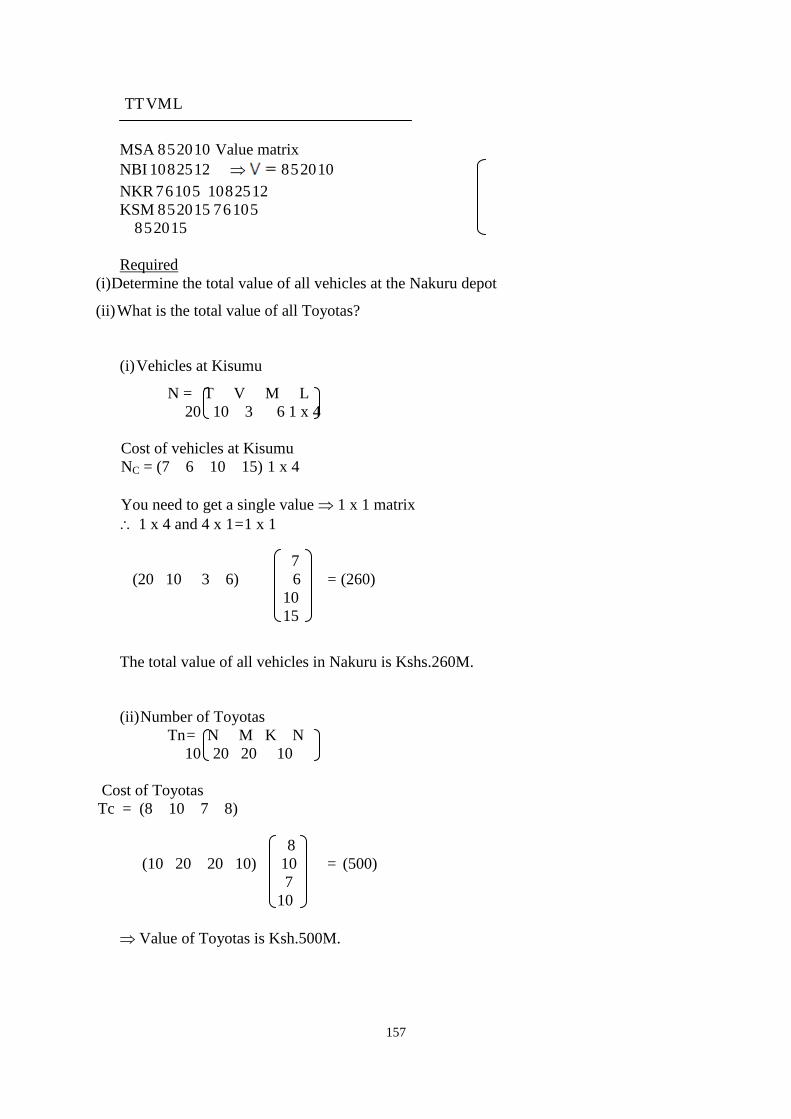
157

TT V M L

MSA 8 5 20 10 Value matrix

NBI 10 8 25 12 8 5 20 10

NKR 7 6 10 5 10 8 25 12

KSM 8 5 20 15 7 6 10 5

8 5 20 15

Required

(i) Determine the total value of all vehicles at the Nakuru depot

(ii) What is the total value of all Toyotas?

(i) Vehicles at Kisumu

N = T V M L

20 10 3 6 1 x 4

Cost of vehicles at Kisumu

NC = (7 6 10 15) 1 x 4

You need to get a single value 1 x 1 matrix

1 x 4 and 4 x 1 = 1 x 1

7

(20 10 3 6) 6 = (260)

10

15

The total value of all vehicles in Nakuru is Kshs.260M.

(ii) Number of Toyotas

Tn = N M K N

10 20 20 10

Cost of Toyotas

Tc = (8 10 7 8)

8

(10 20 20 10) 10 = (500)

7

10

Value of Toyotas is Ksh.500M.

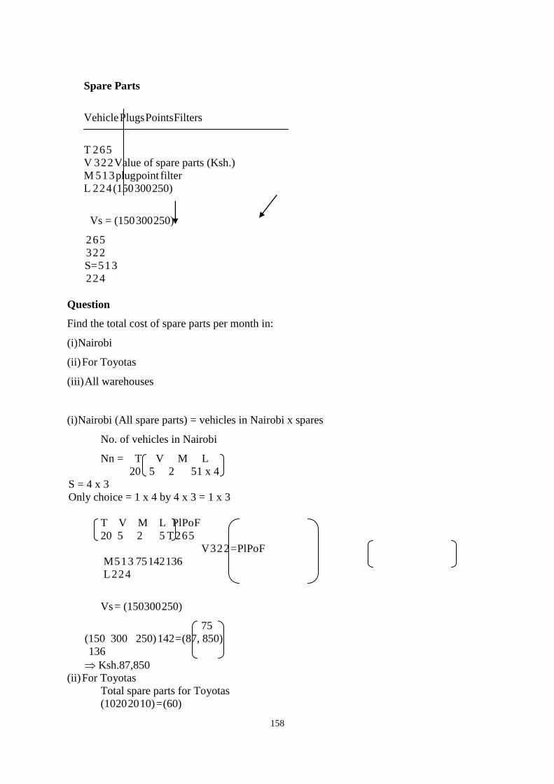
158

Spare Parts

Vehicle Plugs Points Filters

T 2 6 5

V 3 2 2 Value of spare parts (Ksh.)

M 5 1 3 plug point filter

L 2 2 4 (150 300 250)

Vs = (150 300 250)

2 6 5

3 2 2

S= 5 1 3

2 2 4

Question

Find the total cost of spare parts per month in:

(i) Nairobi

(ii) For Toyotas

(iii) All warehouses

(i) Nairobi (All spare parts) = vehicles in Nairobi x spares

No. of vehicles in Nairobi

Nn = T V M L

20 5 2 5 1 x 4

S = 4 x 3

Only choice = 1 x 4 by 4 x 3 = 1 x 3

T V M L Pl Po F

20 5 2 5 T 2 6 5

V 3 2 2 = Pl Po F

M 5 1 3 75 142 136

L 2 2 4

Vs = (150 300 250)

75

(150 300 250) 142 = (87, 850)

136

Ksh.87,850

(ii) For Toyotas

Total spare parts for Toyotas

(10 20 20 10) = (60)

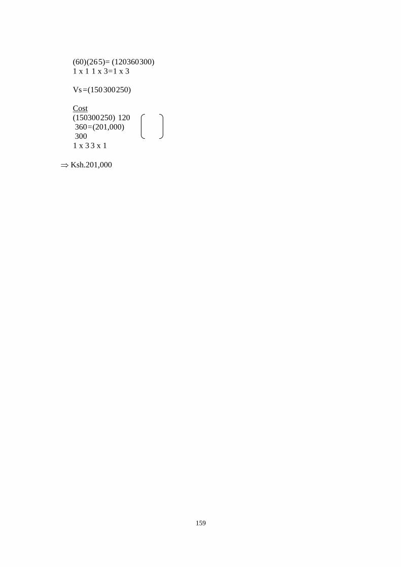
159

(60) (2 6 5) = (120 360 300)

1 x 1 1 x 3 = 1 x 3

Vs = (150 300 250)

Cost

(150300 250) 120

360 = (201,000)

300

1 x 3 3 x 1

Ksh.201,000

160

LECTURE THIRTEEN

MATRICES: MARKOV PROCESS AND INPUT-OUTPUT ANALYSIS

Lecture Outlines

13.1 Introduction

13.2 Objectives

13.3 Markov Analysis (Markov Process / Chains)

13.3.1 Assumptions of Markovian process

13.3.2 Applications of Markovian process

13.4 Input-Output Analysis

13.4.1 Input – output table

13.4.2 Data Requirements

13.4.3 Model derivation

13.5 Summary

13.6 Activities

13.1 Introduction

Welcome to Lecture 13 in this course unit. In this lecture we are going to learn about two

areas of matrix application. Consequently, the lecture will have two parts.

The first part will cover markov(ian) process while the second part will entail input – output

analysis and how they relate to business decision making and management.

13.2 Objectives

At the end of this lecture you should be able to:

1. Define a Markov process and explain its assumptions

2. Apply Markov process in solving business problems

3. Define an input/output model and explain its assumptions

4. Apply input/output model in solving business problems

13.3 Markov Analysis (Markov Process / Chains)

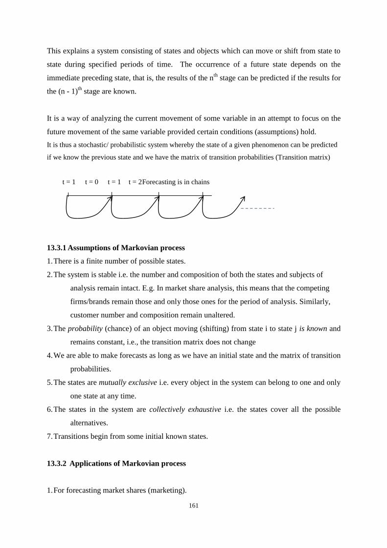
161

This explains a system consisting of states and objects which can move or shift from state to

state during specified periods of time. The occurrence of a future state depends on the

immediate preceding state, that is, the results of the nth

stage can be predicted if the results for

the (n - 1)th

stage are known.

It is a way of analyzing the current movement of some variable in an attempt to focus on the

future movement of the same variable provided certain conditions (assumptions) hold.

It is thus a stochastic/ probabilistic system whereby the state of a given phenomenon can be predicted

if we know the previous state and we have the matrix of transition probabilities (Transition matrix)

t = 1 t = 0 t = 1 t = 2 Forecasting is in chains

13.3.1 Assumptions of Markovian process

1. There is a finite number of possible states.

2. The system is stable i.e. the number and composition of both the states and subjects of

analysis remain intact. E.g. In market share analysis, this means that the competing

firms/brands remain those and only those ones for the period of analysis. Similarly,

customer number and composition remain unaltered.

3. The probability (chance) of an object moving (shifting) from state i to state j is known and

remains constant, i.e., the transition matrix does not change

4. We are able to make forecasts as long as we have an initial state and the matrix of transition

probabilities.

5. The states are mutually exclusive i.e. every object in the system can belong to one and only

one state at any time.

6. The states in the system are collectively exhaustive i.e. the states cover all the possible

alternatives.

7. Transitions begin from some initial known states.

13.3.2 Applications of Markovian process

1. For forecasting market shares (marketing).

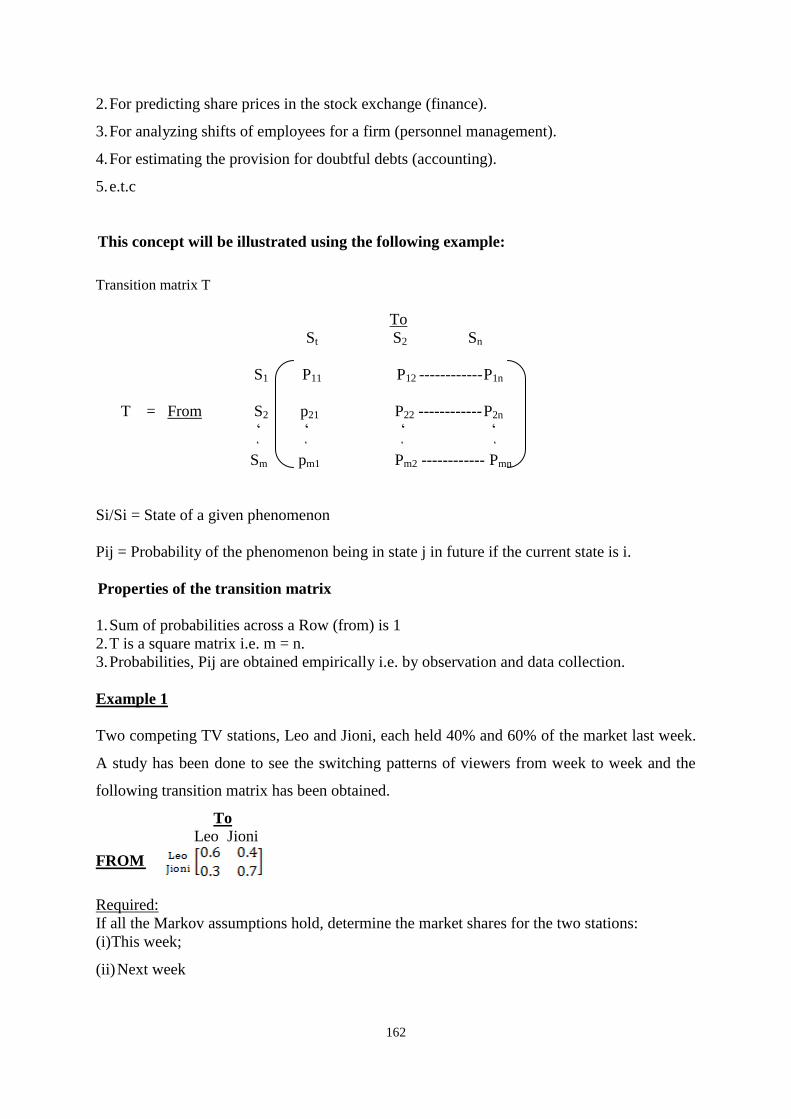
162

2. For predicting share prices in the stock exchange (finance).

3. For analyzing shifts of employees for a firm (personnel management).

4. For estimating the provision for doubtful debts (accounting).

5. e.t.c

This concept will be illustrated using the following example:

Transition matrix T

To

St S2 Sn

S1 P11 P12 ------------ P1n

T = From S2 p21 P22 ------------ P2n

‘ ‘ ‘ ‘

‘ ‘ ‘ ‘

Sm pm1 Pm2 ------------ Pmn

Si/Si = State of a given phenomenon

Pij = Probability of the phenomenon being in state j in future if the current state is i.

Properties of the transition matrix

1. Sum of probabilities across a Row (from) is 1

2. T is a square matrix i.e. m = n.

3. Probabilities, Pij are obtained empirically i.e. by observation and data collection.

Example 1

Two competing TV stations, Leo and Jioni, each held 40% and 60% of the market last week.

A study has been done to see the switching patterns of viewers from week to week and the

following transition matrix has been obtained.

To

Leo Jioni

FROM

Required:

If all the Markov assumptions hold, determine the market shares for the two stations:

(i) This week;

(ii) Next week

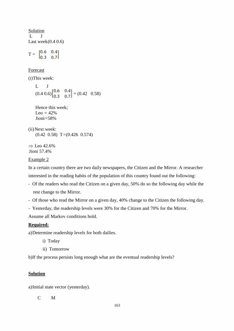
163

Solution

L J

Last week (0.4 0.6)

T =

Forecast

(i) This week:

L J

(0.4 0.6) = (0.42 0.58)

Hence this week;

Leo = 42%

Jioni = 58%

(ii) Next week:

(0.42 0.58) T = (0.426 0.574)

Leo 42.6%

Jioni 57.4%

Example 2

In a certain country there are two daily newspapers, the Citizen and the Mirror. A researcher

interested in the reading habits of the population of this country found out the following:

- Of the readers who read the Citizen on a given day, 50% do so the following day while the

rest change to the Mirror.

- Of those who read the Mirror on a given day, 40% change to the Citizen the following day.

- Yesterday, the readership levels were 30% for the Citizen and 70% for the Mirror.

Assume all Markov conditions hold.

Required:

a) Determine readership levels for both dailies.

i) Today

ii) Tomorrow

b) If the process persists long enough what are the eventual readership levels?

Solution

a) Initial state vector (yesterday).

C M

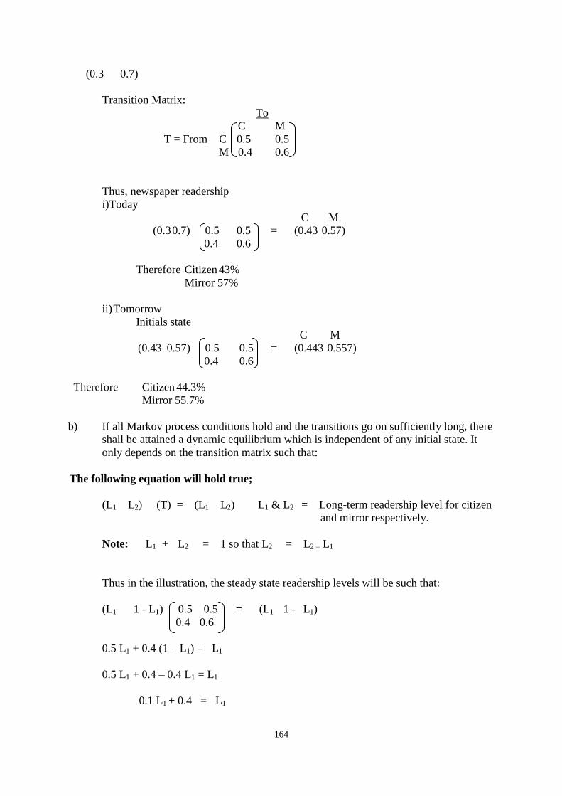
164

(0.3 0.7)

Transition Matrix:

To

C M

T = From C 0.5 0.5

M 0.4 0.6

Thus, newspaper readership

i) Today

C M

(0.3 0.7) 0.5 0.5 = (0.43 0.57)

0.4 0.6

Therefore Citizen 43%

Mirror 57%

ii) Tomorrow

Initials state

C M

(0.43 0.57) 0.5 0.5 = (0.443 0.557)

0.4 0.6

Therefore Citizen 44.3%

Mirror 55.7%

b) If all Markov process conditions hold and the transitions go on sufficiently long, there

shall be attained a dynamic equilibrium which is independent of any initial state. It

only depends on the transition matrix such that:

The following equation will hold true;

(L1 L2) (T) = (L1 L2) L1 & L2 = Long-term readership level for citizen

and mirror respectively.

Note: L1 + L2 = 1 so that L2 = L2 – L1

Thus in the illustration, the steady state readership levels will be such that:

(L1 1 - L1) 0.5 0.5 = (L1 1 - L1)

0.4 0.6

0.5 L1 + 0.4 (1 – L1) = L1

0.5 L1 + 0.4 – 0.4 L1 = L1

0.1 L1 + 0.4 = L1

165

0.4 = L1 – 0.1 L1

0.4 = 0.9 L1

L1 = 9.0

4.0

L1 = 0.44

L2 = 1 – L1 = 1 – 0.44 = 0.56

Therefore Citizen = 44%

Mirror = 56%

13.4 INPUT-OUTPUT ANALYSIS

Input-output analysis is concerned with the study of interdependence between organizational

units, e.g. sectors in an economy. Sectors in the economy are interdependent in the sense that

each requires the output of the others in-order to operate/produce its own output.

Example:

Consider an economy with 3 sectors: agricultural, manufacturing and services with

transactions in a given year as shown below (figures in billon of shillings).

13.4.1 Input-output table

User of inputs

Agriculture Manufacturing Services Final

Dd

Total

output

Agriculture

Producer of Manufacturing

Outputs Services

20 0 27

30 32 9

10 40 18

53

9

22

100

80

90

Primary output 40 8 36

Total input 100 80 90 270

GDP

The input /output table has 5 parts or components:

1. Intermediate demand – This represents the worth of goods and services which is

reused within the production sectors as further input. This is inter-sectoral demand

and specifically excludes final demand.

Also called intermediate or intersectoral demand.

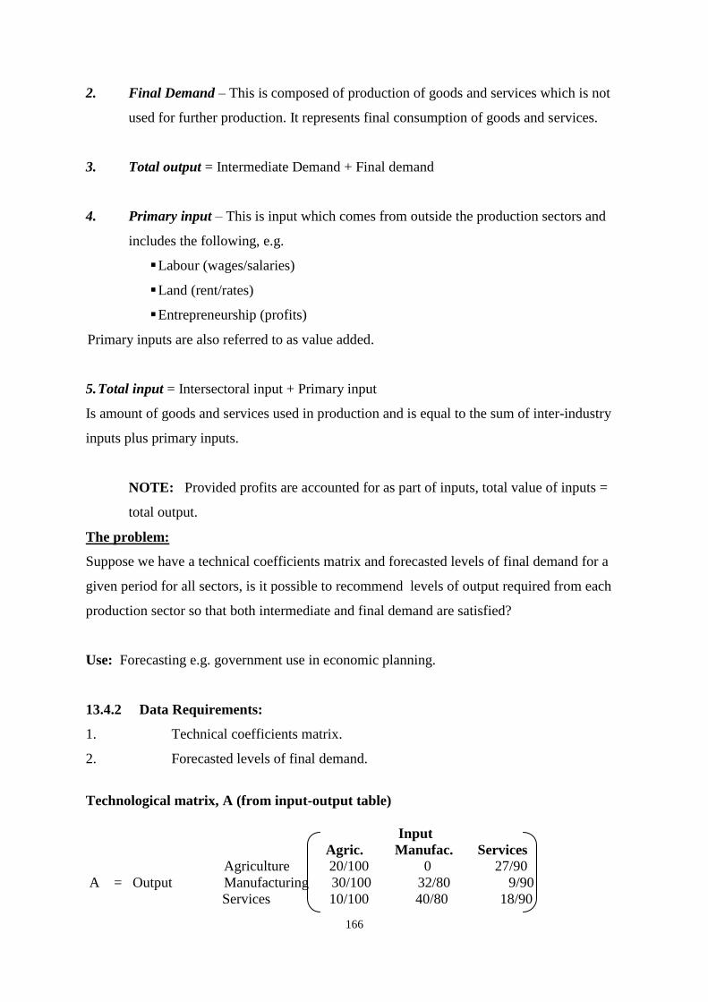
166

2. Final Demand – This is composed of production of goods and services which is not

used for further production. It represents final consumption of goods and services.

3. Total output = Intermediate Demand + Final demand

4. Primary input – This is input which comes from outside the production sectors and

includes the following, e.g.

Labour (wages/salaries)

Land (rent/rates)

Entrepreneurship (profits)

Primary inputs are also referred to as value added.

5. Total input = Intersectoral input + Primary input

Is amount of goods and services used in production and is equal to the sum of inter-industry

inputs plus primary inputs.

NOTE: Provided profits are accounted for as part of inputs, total value of inputs =

total output.

The problem:

Suppose we have a technical coefficients matrix and forecasted levels of final demand for a

given period for all sectors, is it possible to recommend levels of output required from each

production sector so that both intermediate and final demand are satisfied?

Use: Forecasting e.g. government use in economic planning.

13.4.2 Data Requirements:

1. Technical coefficients matrix.

2. Forecasted levels of final demand.

Technological matrix, A (from input-output table)

Input

Agric. Manufac. Services

Agriculture 20/100 0 27/90

A = Output Manufacturing 30/100 32/80 9/90

Services 10/100 40/80 18/90

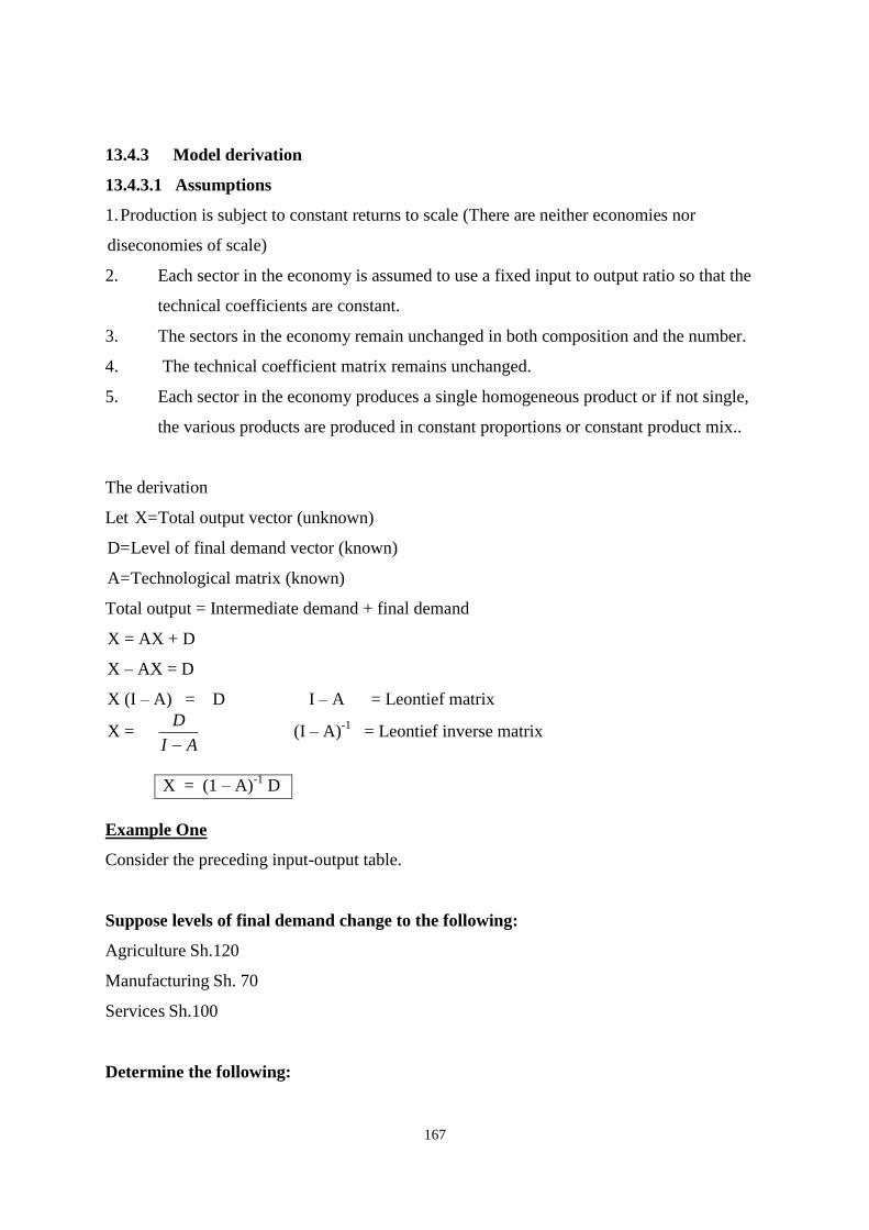
167

13.4.3 Model derivation

13.4.3.1 Assumptions

1. Production is subject to constant returns to scale (There are neither economies nor

diseconomies of scale)

2. Each sector in the economy is assumed to use a fixed input to output ratio so that the

technical coefficients are constant.

3. The sectors in the economy remain unchanged in both composition and the number.

4. The technical coefficient matrix remains unchanged.

5. Each sector in the economy produces a single homogeneous product or if not single,

the various products are produced in constant proportions or constant product mix..

The derivation

Let X = Total output vector (unknown)

D = Level of final demand vector (known)

A = Technological matrix (known)

Total output = Intermediate demand + final demand

X = AX + D

X – AX = D

X (I – A) = D I – A = Leontief matrix

X = AI

D

(I – A)

-1 = Leontief inverse matrix

X = (1 – A)-1

D

Example One

Consider the preceding input-output table.

Suppose levels of final demand change to the following:

Agriculture Sh.120

Manufacturing Sh. 70

Service s Sh.100

Determine the following:

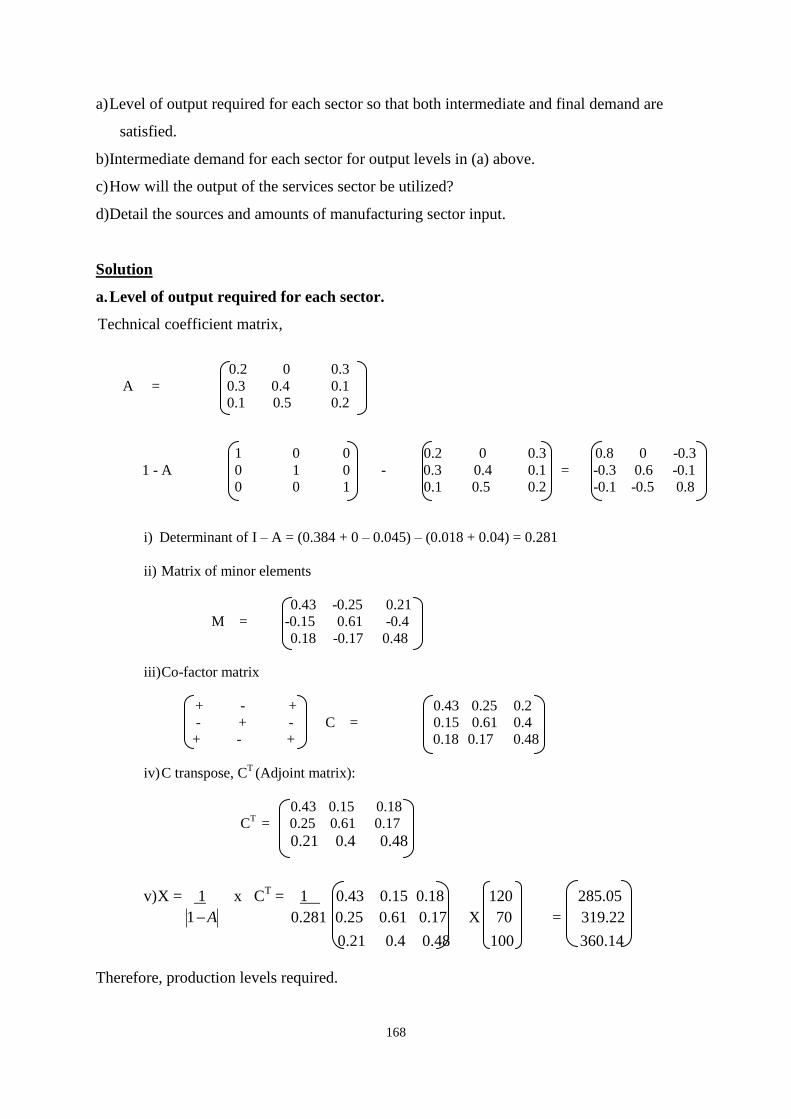
168

a) Level of output required for each sector so that both intermediate and final demand are

satisfied.

b) Intermediate demand for each sector for output levels in (a) above.

c) How will the output of the services sector be utilized?

d) Detail the sources and amounts of manufacturing sector input.

Solution

a. Level of output required for each sector.

Technical coefficient matrix,

0.2 0 0.3

A = 0.3 0.4 0.1

0.1 0.5 0.2

1 0 0 0.2 0 0.3 0.8 0 -0.3

1 - A 0 1 0 - 0.3 0.4 0.1 = -0.3 0.6 -0.1

0 0 1 0.1 0.5 0.2 -0.1 -0.5 0.8

i) Determinant of I – A = (0.384 + 0 – 0.045) – (0.018 + 0.04) = 0.281

ii) Matrix of minor elements

0.43 -0.25 0.21

M = -0.15 0.61 -0.4

0.18 -0.17 0.48

iii) Co-factor matrix

+ - + 0.43 0.25 0.2

- + - C = 0.15 0.61 0.4

+ - + 0.18 0.17 0.48

iv) C transpose, CT

(Adjoint matrix):

0.43 0.15 0.18

CT = 0.25 0.61 0.17

0.21 0.4 0.48

v) X = 1 x CT = 1 0.43 0.15 0.18 120 285.05

A1 0.281 0.25 0.61 0.17 X 70 = 319.22

0.21 0.4 0.48 100 360.14

Therefore, production levels required.

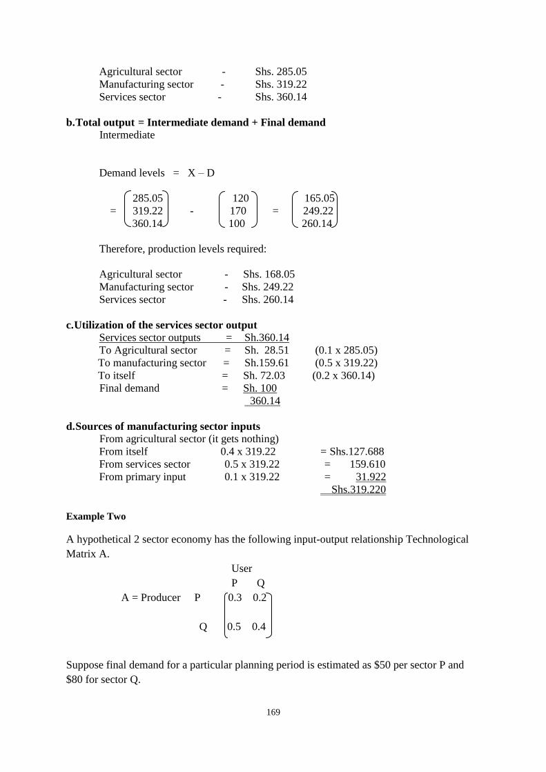
169

Agricultural sector - Shs. 285.05

Manufacturing sector - Shs. 319.22

Services sector - Shs. 360.14

b. Total output = Intermediate demand + Final demand

Intermediate

Demand levels = X – D

285.05 120 165.05

= 319.22 - 170 = 249.22

360.14 100 260.14

Therefore, production levels required:

Agricultural sector - Shs. 168.05

Manufacturing sector - Shs. 249.22

Services sector - Shs. 260.14

c. Utilization of the services sector output

Services sector outputs = Sh.360.14

To Agricultural sector = Sh. 28.51 (0.1 x 285.05)

To manufacturing sector = Sh.159.61 (0.5 x 319.22)

To itself = Sh. 72.03 (0.2 x 360.14)

Final demand = Sh. 100

360.14

d. Sources of manufacturing sector inputs

From agricultural sector (it gets nothing)

From itself 0.4 x 319.22 = Shs.127.688

From services sector 0.5 x 319.22 = 159.610

From primary input 0.1 x 319.22 = 31.922

Shs.319.220

Example Two

A hypothetical 2 sector economy has the following input-output relationship Technological

Matrix A.

User

P Q

A = Producer P 0.3 0.2

Q 0.5 0.4

Suppose final demand for a particular planning period is estimated as $50 per sector P and

$80 for sector Q.

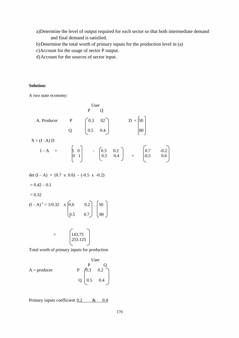
170

a) Determine the level of output required for each sector so that both intermediate demand

and final demand is satisfied.

b) Determine the total worth of primary inputs for the production level in (a)

c) Account for the usage of sector P output.

d) Account for the sources of sector input.

Solution:

A two state economy:

User

P Q

A. Producer P 0.3 02 D = 50

Q 0.5 0.4 80

X = (I –A) D

I – A = 1 0 - 0.3 0.2 0.7 -0.2

0 1 0.5 0.4 = -0.5 0.6

det (I – A) = (0.7 x 0.6) - (-0.5 x -0.2)

= 0.42 – 0.1

= 0.32

(I – A)-1

= 1/0.32 x 0.6 0.2 50

0.5 0.7 80

= 143.75

253.125

Total worth of primary inputs for production

User

P Q

A = producer P 0.3 0.2

Q 0.5 0.4

Primary inputs coefficient 0.2 & 0.4

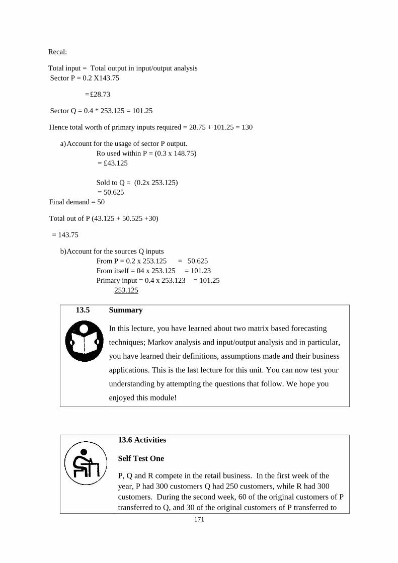
171

Recal:

Total input = Total output in input/output analysis

Sector P = 0.2 X143.75

= £28.73

Sector Q = 0.4 * 253.125 = 101.25

Hence total worth of primary inputs required = 28.75 + 101.25 = 130

a) Account for the usage of sector P output.

Ro used within P = (0.3 x 148.75)

= £43.125

Sold to Q = (0.2x 253.125)

= 50.625

Final demand = 50

Total out of P (43.125 + 50.525 +30)

= 143.75

b) Account for the sources Q inputs

From P = 0.2 x 253.125 = 50.625

From itself = 04 x 253.125 = 101.23

Primary input = 0.4 x 253.123 = 101.25

253.125

13.5

Summary

In this lecture, you have learned about two matrix based forecasting

techniques; Markov analysis and input/output analysis and in particular,

you have learned their definitions, assumptions made and their business

applications. This is the last lecture for this unit. You can now test your

understanding by attempting the questions that follow. We hope you

enjoyed this module!

13.6 Activities

Self Test One

P, Q and R compete in the retail business. In the first week of the

year, P had 300 customers Q had 250 customers, while R had 300

customers. During the second week, 60 of the original customers of P

transferred to Q, and 30 of the original customers of P transferred to

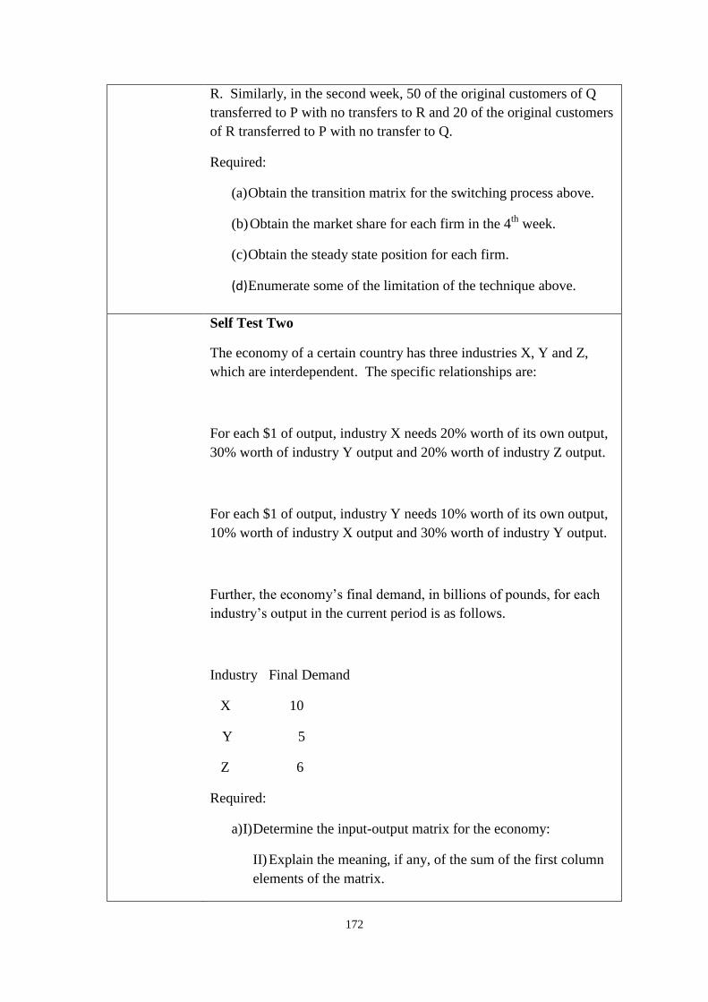
172

R. Similarly, in the second week, 50 of the original customers of Q

transferred to P with no transfers to R and 20 of the original customers

of R transferred to P with no transfer to Q.

Required:

(a) Obtain the transition matrix for the switching process above.

(b) Obtain the market share for each firm in the 4th

week.

(c) Obtain the steady state position for each firm.

(d) Enumerate some of the limitation of the technique above.

Self Test Two

The economy of a certain country has three industries X, Y and Z,

which are interdependent. The specific relationships are:

For each $1 of output, industry X needs 20% worth of its own output,

30% worth of industry Y output and 20% worth of industry Z output.

For each $1 of output, industry Y needs 10% worth of its own output,

10% worth of industry X output and 30% worth of industry Y output.

Further, the economy’s final demand, in billions of pounds, for each

industry’s output in the current period is as follows.

Industry Final Demand

X 10

Y 5

Z 6

Required:

a) I) Determine the input-output matrix for the economy:

II) Explain the meaning, if any, of the sum of the first column

elements of the matrix.

173

iii) Explain the meaning, if any, of the sum of the third row

elements of the matrix.

b) Determine the output level for each industry so that the current

final demand can be satisfied.

c) Determine the total worth of intermediate demand for output

levels in (b) above.

d) Determine, and explain, the level of primary production

required for (b) above, for each industry.